1 Introduction

Probability measures are widely used to represent objects of interest across various research fields. For instance, in natural language processing, documents can be viewed as distributions over words (Sparck Jones, 1972; Kusner et al., 2015), or distributions over topics (Blei et al., 2003; Yurochkin et al., 2019). In computer vision and graphics, 3D objects are often represented as point clouds, which are distributions of 3D data points (Achlioptas et al., 2018; Hua et al., 2018; Wang et al., 2019; Wu et al., 2019). In topological data analysis (TDA), persistence diagrams (PD) are used to represent complex structural objects (Rieck et al., 2019; Zhao & Wang, 2019; Divol & Lacombe, 2021). Specifically, PDs can be regarded as distributions of 2D data points, where each point characterizes the birth and death time of a particular topological feature (Edelsbrunner & Harer, 2008).

Integral probability metrics (IPMs) are a powerful class of distances for comparing probability measures (Müller, 1997). Essentially, IPMs identify a critic function (or witness function) that maximizes the discrimination between data points sampled from two input probability measures. IPMs have been applied in numerous theoretical studies and practical applications (Sriperumbudur et al., 2009; Gretton et al., 2012; Peyré & Cuturi, 2019; Liang, 2019; Uppal et al., 2019, 2020; Nadjahi et al., 2020; Kolouri et al., 2020).

In this work, we study Sobolev IPM problem for probability measures supported on a graph. Sobolev IPM is an important instance of IPM, and is obtained by constraining the critic function within a unit ball defined by the Sobolev norm (Adams & Fournier, 2003). Sobolev IPM plays a crucial role in several theoretical works, such as analyzing convergence rates of density estimation with generative adversarial networks (GANs) and studying error bounds for deep ReLU discriminator networks in GANs (Liang, 2017, 2021; Singh et al., 2018). However, to our knowledge, a long-standing challenge for Sobolev IPM is that there are no efficient algorithmic approaches to compute it effectively which limits its applications in practice. To address this issue, we propose a novel regularization for the Sobolev IPM problem. By leveraging the graph structure, we demonstrate that the regularized Sobolev IPM yields a closed-form expression for fast computation, thereby paving the way for its application in various domains, even for large-scale settings.

Contribution.

Our contributions are three-fold:

• We propose a novel regularization for Sobolev IPM that provides a closed-form expression for fast computation, overcoming the long-standing computational challenge and facilitating its application, particularly in large-scale settings.

• We prove that the regularized Sobolev IPM is a metric and show its equivalence to the original Sobolev IPM. Additionally, we establish its connections to Sobolev transport (ST) which is a scalable variant of optimal transport (OT) for measures on a graph, and also its connection to the traditional OT on a graph.

• We demonstrate that the regularized Sobolev IPM is negative definite. We then design positive definite kernels based on the regularized Sobolev IPM and provide preliminary evidence of their advantages in document classification and topological data analysis (TDA).

Organization.

In §2, we introduce the notations used throughout our proposals. Section §3 details our novel regularization for Sobolev IPM. In §4, we prove the metric property for the regularized Sobolev IPM and establish its connection to the original Sobolev IPM, ST, and OT on a graph. Additionally, we demonstrate the negative definiteness for the regularized Sobolev IPM and propose positive definite kernels based on it. Section §5 discusses related works. In §6, we empirically illustrate the computational advantages of the regularized Sobolev IPM and provide preliminary evidence of its benefits in document classification and TDA. Finally, §7 offers concluding remarks. Proofs for theoretical results and additional materials are deferred to the Appendices.

2 Preliminaries

In this section, we briefly review the graph setting for probability measures. We also introduce some notations and functional spaces on the graph.

Graph. We follow the same graph setting in Le et al. (2022) for measures and functions. Precisely, let $V,E$ denote the sets of nodes and edges respectively. We consider a connected, undirected, and physical graph ${\mathbb{G}}=(V,E)$ with positive edge lengths $\{w_{e}\}_{e\in E}$. The continuous graph setting is adopted, i.e. ${\mathbb{G}}$ is regarded as the collection of all nodes in $V$ together with all points forming the edges in $E$. Additionally, ${\mathbb{G}}$ is equipped with the graph metric $d_{{\mathbb{G}}}(x,y)$, which is defined as the length of the shortest path connecting $x$ and $y$ in ${\mathbb{G}}$. We assume that there exists a fixed root node $z_{0}\in V$ such that the shortest path between $z_{0}$ and $x$ is unique for any $x\in{\mathbb{G}}$, i.e., the uniqueness property of the shortest paths (Le et al., 2022).

Denote $[x,z]$ as the shortest path between $x$ and $z$ in ${\mathbb{G}}$. Then for given $x\in{\mathbb{G}}$ and edge $e\in E$, we define the sets $\Lambda(x)$ and $\gamma_{e}$ as follows

$$\Lambda(x):=\big{\{}y\in{\mathbb{G}}:\,x\in[z_{0},y]\big{\}},$$

$$\gamma_{e}:=\big{\{}y\in{\mathbb{G}}:\,e\subseteq[z_{0},y]\big{\}}.$$ (1)

Measures and functions on graph. Let ${\mathcal{P}}({\mathbb{G}})$ (resp.$\,{\mathcal{P}}({\mathbb{G}}\times{\mathbb{G}})$) denote the set of all nonnegative Borel measures on ${\mathbb{G}}$ (resp.$\,{\mathbb{G}}\times{\mathbb{G}}$) with a finite mass.

By a continuous function $f$ on ${\mathbb{G}}$, we mean that $f:{\mathbb{G}}\to\mathbb{R}$ is continuous w.r.t. the topology on ${\mathbb{G}}$ induced by the Euclidean distance. Henceforth, $C({\mathbb{G}})$ stands for the set of all continuous functions on ${\mathbb{G}}$. Similar notation is used for continuous functions on ${\mathbb{G}}\times{\mathbb{G}}$.

For a nonnegative Borel measure $\lambda$ on ${\mathbb{G}}$ and $1\leq p<\infty$, let $L^{p}({\mathbb{G}},\lambda)$ denote the space of all Borel measurable functions $f:{\mathbb{G}}\to\mathbb{R}$ such that $\int_{\mathbb{G}}|f(x)|^{p}\lambda(\mathrm{d}x)<\infty$. Then $L^{p}({\mathbb{G}},\lambda)$ is a normed space with the norm being defined by

$$\|f\|_{L^{p}}:=\left(\int_{\mathbb{G}}|f(x)|^{p}\lambda(\mathrm{d}x)\right)^{\frac{1}{p}}.$$

Additionally, let $\hat{w}$ be a positive weight function on ${\mathbb{G}}$, i.e., $\hat{w}(x)>0$ for every $x\in{\mathbb{G}}$. Consider the weighted $L_{\hat{w}}^{p}({\mathbb{G}},\lambda)$ as the space of all Borel measurable functions $f:{\mathbb{G}}\to\mathbb{R}$ such that $\int_{\mathbb{G}}\hat{w}(x)|f(x)|^{p}\lambda(\mathrm{d}x)<\infty$. It is a normed space with the following weighted $L^{p}$-norm

$$\|f\|_{L_{\hat{w}}^{p}}:=\left(\int_{\mathbb{G}}\hat{w}(x)|f(x)|^{p}\lambda(\mathrm{d}x)\right)^{\frac{1}{p}}.$$

The spaces $L^{p}({\mathbb{G}},\lambda)$, $L_{\hat{w}}^{p}({\mathbb{G}},\lambda)$ and their corresponding norms can also be defined for the case $p=\infty$. Further details are placed in Appendix §B.1.

3 Regularized Sobolev IPM

In this section, we consider the Sobolev IPM problem for probability measures on a graph. We show that the Sobolev norm of $f$ is equivalent to a weighted $L^{p}$-norm of $f^{\prime}$ with a specific weight function. Then we propose to leverage the weighted $L^{p}$-norm to regularize the Sobolev IPM. It is also demonstrated that a closed-form expression can be derived for the regularized Sobolev IPM.

3.1 Sobolev IPM

We first introduce the graph-based Sobolev space (Le et al., 2022) and its Sobolev norm (Adams & Fournier, 2003). Utilizing these, we then give the definition of Sobolev IPM for probability measures on a graph.

Definition 3.1 (Graph-based Sobolev space (Le et al., 2022)).

Let $\lambda$ be a nonnegative Borel measure on ${\mathbb{G}}$, and let $1\leq p\leq\infty$. A continuous function $f:{\mathbb{G}}\to\mathbb{R}$ is said to belong to the Sobolev space $W^{1,p}({\mathbb{G}},\lambda)$ if there exists a function $h\in L^{p}({\mathbb{G}},\lambda)$ satisfying

$$f(x)-f(z_{0})=\int_{[z_{0},x]}h(y)\lambda(\mathrm{d}y)\quad\forall x\in{\mathbb{G}}.$$ (2)

Such function $h$ is unique in $L^{p}({\mathbb{G}},\lambda)$ and is called the graph derivative of $f$ w.r.t. the measure $\lambda$. The graph derivative of $f\in W^{1,p}({\mathbb{G}},\lambda)$ is denoted as $f^{\prime}\in L^{p}({\mathbb{G}},\lambda)$.

Sobolev norm. $W^{1,p}({\mathbb{G}},\lambda)$ is a normed space with the Sobolev norm (Adams & Fournier, 2003, §3.1) being defined as

$$\left\lVert f\right\rVert_{W^{1,p}}:=\left(\left\lVert f\right\rVert_{L^{p}}^{p}+\left\lVert f^{\prime}\right\rVert_{L^{p}}^{p}\right)^{\frac{1}{p}}.$$ (3)

Additionally, let $W^{1,p}_{0}({\mathbb{G}},\lambda)$ be the subspace consisting of all functions $f$ in $W^{1,p}({\mathbb{G}},\lambda)$ satisfying $f(z_{0})=0$. Denote ${\mathcal{B}}(p):=\left\{f\in W^{1,p}_{0}({\mathbb{G}},\lambda):\left\lVert f\right\rVert_{W^{1,p}}\leq 1\right\}$ as the unit ball in the Sobolev space.

Sobolev IPM.

Sobolev IPM for probability measures on a graph is an instance of the integral probability metric (IPM) where its critic function belongs to the graph-based Sobolev space, and is constrained within the unit ball of that space. More concretely, given a nonnegative Borel measure $\lambda$ on ${\mathbb{G}}$, an exponent $1\leq p\leq\infty$ and its conjugate $p^{\prime}$, the Sobolev IPM between any two probability measures $\mu,\nu\in{\mathcal{P}}({\mathbb{G}})$ is defined as

$${\mathcal{S}}_{p}(\mu,\nu):=\hskip-3.99994pt\sup_{f\in{\mathcal{B}}(p^{\prime})}\hskip-1.99997pt\left|\int_{{\mathbb{G}}}f(x)\mu(\text{d}x)-\int_{{\mathbb{G}}}f(y)\nu(\text{d}y)\right|.$$ (4)

Notice that the quantity inside the absolute signs is unchanged if $f$ is replaced by $f-f(z_{0})$. Thus, we can assume without loss of generality that $f(z_{0})=0$. This is the motivation for our introduction of the Sobolev space $W^{1,p}_{0}({\mathbb{G}},\lambda)$.

Weight function.

Hereafter, we consider the weight function

$$\hat{w}(x):=1+\lambda(\Lambda(x)),\qquad\forall x\in{\mathbb{G}}.$$ (5)

The next result plays the key role in our approach.

Theorem 3.2 (Equivalence).

For a nonnegative Borel measure $\lambda$ on ${\mathbb{G}}$ and $1\leq p<\infty$, let $c_{1}:=\left[\frac{\min(1,\lambda({\mathbb{G}})^{p-1})}{1+\lambda({\mathbb{G}})^{p}}\right]^{\frac{1}{p}}$, and $c_{2}:=\left[\max(1,\lambda({\mathbb{G}})^{p-1})\right]^{\frac{1}{p}}$. Then, we have

$$c_{1}\left\lVert f^{\prime}\right\rVert_{L^{p}_{\hat{w}}}\leq\left\lVert f\right\rVert_{W^{1,p}}\leq c_{2}\left\lVert f^{\prime}\right\rVert_{L^{p}_{\hat{w}}},$$ (6)

for every function $f\in W^{1,p}_{0}({\mathbb{G}},\lambda)$.

The proof is placed in Appendix §A.1.

Relation (6) implies that the Sobolev norm of a critic function $f\in W_{0}^{1,p}({\mathbb{G}},\lambda)$ is equivalent to the weighted $L^{p}$-norm of its gradient $f^{\prime}$. Moreover, the weight function is given explicitly by Equation (5).

3.2 Regularized Sobolev IPM

Based on the equivalent relation given by Theorem 3.2, we propose to regularize the Sobolev IPM (Equation (4)) by relaxing the constraint on the critic function $f$ in the graph-based Sobolev space $W^{1,p^{\prime}}_{0}$. More precisely, instead of $f$ belonging to the unit ball ${\mathcal{B}}(p^{\prime})$ of the Sobolev space, we propose to constraint critic $f$ within the unit ball ${\mathcal{B}}(p^{\prime},\hat{w})$ of the weighted $L^{p^{\prime}}\!$-norm of $f^{\prime}$ with weight function $\hat{w}$. Hereafter, ${\mathcal{B}}(p^{\prime},\hat{w})$ is defined by

$${\mathcal{B}}(p^{\prime},\hat{w}):=\left\{f\in W^{1,p^{\prime}}_{0}\!({\mathbb{G}},\lambda):\left\lVert f^{\prime}\right\rVert_{L^{p^{\prime}}_{\hat{w}}}\leq 1\right\}.$$ (7)

We now formally define the regularized Sobolev IPM between two probability distributions on graph ${\mathbb{G}}$.

Definition 3.3 (Regularized Sobolev IPM on graph).

Let $\lambda$ be a nonnegative Borel measure on ${\mathbb{G}}$ and $1\leq p\leq\infty$. Then for any given probability measures $\mu,\nu\in{\mathcal{P}}({\mathbb{G}})$, the regularized Sobolev IPM is defined as

$$\hat{{\mathcal{S}}}_{p}(\mu,\nu)\hskip-1.00006pt:=\hskip-13.00005pt\sup_{f\in{\mathcal{B}}(p^{\prime},\hat{w})}\hskip-1.99997pt\left|\int_{{\mathbb{G}}}f(x)\mu(\text{d}x)-\int_{{\mathbb{G}}}f(y)\nu(\text{d}y)\right|.\hskip-2.5pt$$ (8)

The following result shows that the regularized Sobolev IPM yields a closed-form expression.

Theorem 3.4 (Closed-form expression).

Let $\lambda$ be any nonnegative Borel measure on ${\mathbb{G}}$, and $1\leq p<\infty$. Then

$$\hat{{\mathcal{S}}}_{p}(\mu,\nu)^{p}\hskip-1.00006pt=\hskip-3.99994pt\int_{{\mathbb{G}}}\hskip-3.00003pt\hat{w}(x)^{1-p}\left|\mu(\Lambda(x))-\nu(\Lambda(x))\right|^{p}\lambda(\mathrm{d}x).\hskip-1.79993pt$$ (9)

The proof is placed in Appendix §A.2.

We note that in identity (9), both the subgraph $\Lambda(x)$ (Equation (2)) and the weight function $\hat{w}(x)$ (Equation (5)) depend on input point $x$ under the integral over ${\mathbb{G}}$.

For practical applications, we next derive an explicit formula for the integral over graph ${\mathbb{G}}$ in Equation (9) when the input probability measures are supported on nodes $V$ of graph ${\mathbb{G}}$. This gives an efficient method for computing the regularized Sobolev IPM $\hat{{\mathcal{S}}}_{p}$. Note that to achieve this result, we use the length measure on graph ${\mathbb{G}}$ (Le et al., 2022) for the nonnegative Borel measure $\lambda$, i.e., we have $\lambda([x,z])=d_{{\mathbb{G}}}(x,z),\forall x,z\in{\mathbb{G}}$. We summarize the result in the following theorem.

Theorem 3.5 (Discrete case).

Let $\lambda$ be the length measure on ${\mathbb{G}}$, and $1\leq p<\infty$. Suppose that $\mu,\nu\in{\mathcal{P}}({\mathbb{G}})$ are supported on nodes $V$ of graph ${\mathbb{G}}$. Then we have

$$\hat{{\mathcal{S}}}_{p}(\mu,\nu)=\left(\sum_{e\in E}\beta_{e}\left|\mu(\gamma_{e})-\nu(\gamma_{e})\right|^{p}\right)^{\frac{1}{p}},$$ (10)

where for each edge $e\in E$ of graph ${\mathbb{G}}$, the number $\beta_{e}$ is given by

$$\hskip-1.00006pt\beta_{e}:=\left\{\begin{array}[]{ll}\log{\left(1+\frac{w_{e}}{1+\lambda(\gamma_{e})}\right)}&\mbox{if }p=2\hskip-11.00008pt\\ \frac{\left(1+\lambda(\gamma_{e})+w_{e}\right)^{2-p}-\left(1+\lambda(\gamma_{e})\right)^{2-p}}{2-p}&\text{otherwise.}\hskip-11.00008pt\end{array}\right.$$ (11)

The proof is placed in Appendix §A.3.

Remark 3.6 (Non-physical graph).

We assumed that ${\mathbb{G}}$ is a physical graph in §2. Nevertheless, when input measures are supported on nodes $V$ of graph ${\mathbb{G}}$, and $\lambda$ is a length measure of graph ${\mathbb{G}}$, the regularized Sobolev IPM $\hat{{\mathcal{S}}}_{p}$ does not depend on this physical assumption as illustrated in Theorem 3.5. Indeed, it only depends on the graph structure $(V,E)$ and edge weights $w_{e}$. Therefore, we can apply the regularized Sobolev IPM for non-physical graph ${\mathbb{G}}$.

Preprocessing. For the computation of the regularized Sobolev IPM $\hat{{\mathcal{S}}}_{p}$ in Equation (10), observe that the set $\gamma_{e}$ (see Equation (2)) and $\beta_{e}$ (see Equation (11)) can be precomputed for all edges $e$ in ${\mathbb{G}}$. Notably, the preprocessing procedure is only involved graph ${\mathbb{G}}$, and it is independent of the input probability measures. As a consequence, we only need to perform this preprocessing procedure once, regardless of the number of input pairs of probability measures that are evaluated by $\hat{{\mathcal{S}}}_{p}$ in applications. More precisely, we apply the Dijkstra algorithm to recompute the shortest paths from root node $z_{0}$ to all other input supports (or vertices) with complexity $\mathcal{O}(|E|+|V|\log{|V|})$ where we write $|\cdot|$ for the set cardinality. Then, we can evaluate $\gamma_{e}$ and $\beta_{e}$ for each edge $e$ in $E$.

Sparsity of subgraph $\gamma_{e}$ in ${\mathbb{G}}$. Denote $\text{supp}(\mu)$ as the set of supports of measure $\mu$. For any $x\in\text{supp}(\mu)$, its mass is accumulated into $\mu(\gamma_{e})$ if and only if $e\subseteq[z_{0},x]$ (Le et al., 2022). Therefore, let define $E_{\mu,\nu}\subseteq E$ as follows

$$E_{\mu,\nu}\hskip-1.99997pt:=\hskip-1.99997pt\left\{e\!\in\!E\mid\exists z\!\in\!(\text{supp}(\mu)\cup\text{supp}(\nu)),e\subseteq[z_{0},z]\right\}.$$

Then, in fact, we can remove all edges $e\in E\setminus E_{\mu,\nu}$ in the summation in Equation (10) for the computation of the regularized Sobolev IPM $\hat{{\mathcal{S}}}_{p}$. As the result of this sparsity property, the computational complexity of $\hat{{\mathcal{S}}}_{p}$ is reduced to $\mathcal{O}(|E_{\mu,\nu}|)$.

4 Properties of Regularized Sobolev IPM

4.1 Metric and Its Relations

Metrization.

We prove that the regularized Sobolev IPM is a metric.

Theorem 4.1 (Metrization).

For any $1\leq p\leq\infty$, the regularized Sobolev IPM $\hat{{\mathcal{S}}}_{p}$ is a metric on the space ${\mathcal{P}}({\mathbb{G}})$ of probability measures on graph ${\mathbb{G}}$.

The proof is placed in Appendix §A.4.

Connection to the original Sobolev IPM.

We next show that the regularized Sobolev IPM is equivalent to the original Sobolev IPM.

Theorem 4.2 (Relation with original Sobolev IPM).

For a nonnegative Borel measure $\lambda$ on ${\mathbb{G}}$, $1\leq p<\infty$, we have

$$c_{1}\,{\mathcal{S}}_{p}(\mu,\nu)\leq\hat{{\mathcal{S}}}_{p}(\mu,\nu)\leq c_{2}\,{\mathcal{S}}_{p}(\mu,\nu)$$ (12)

for every $\mu,\nu\in{\mathcal{P}}({\mathbb{G}})$, where $c_{1},c_{2}$ are constants defined in Theorem 3.2. Hence, the regularized Sobolev IPM is equivalent to the original Sobolev IPM.

The proof is placed in Appendix §A.5.

Connection to the Sobolev transport (Le et al., 2022).

For $1\leq p<\infty$, let $\mathcal{ST}_{\!p}$ be the $p$-order Sobolev transport, which is a scalable variant of optimal transport for measures on a graph (Le et al., 2022). The next result provides the relation between our regularized Sobolev IPM $\hat{\mathcal{S}}_{p}$ and the Sobolev transport $\mathcal{ST}_{\!p}$.

Proposition 4.3 (Relation with Sobolev transport).

For a nonnegative Borel measure $\lambda$ on ${\mathbb{G}}$, $1\leq p<\infty$, we have

$$(1+\lambda({{\mathbb{G}}}))^{\frac{1-p}{p}}\mathcal{ST}_{\!p}(\mu,\nu)\leq\hat{{\mathcal{S}}}_{p}(\mu,\nu)\leq\mathcal{ST}_{\!p}(\mu,\nu)$$ (13)

for every $\mu,\nu\in{\mathcal{P}}({\mathbb{G}})$. Hence, the regularized Sobolev IPM is equivalent to the Sobolev transport.

The proof is placed in Appendix §A.6.

Regularized Sobolev IPM with different orders.

We establish a relation between different orders for the regularized Sobolev IPM.

Proposition 4.4 (Upper bound).

Let $\lambda$ be any finite and nonnegative Borel measure on ${\mathbb{G}}$. Then we have

$$\hat{{\mathcal{S}}}_{p}(\mu,\nu)\leq\left[\lambda({\mathbb{G}})\left(1+\lambda({\mathbb{G}})\right)\right]^{\frac{1}{p}-\frac{1}{q}}\hat{{\mathcal{S}}}_{q}(\mu,\nu)$$

for any exponents $p$ and $q$ satisfying $1\leq p<q<\infty$.

The proof is placed in Appendix §A.7.

Connection to the Wasserstein distance.

We establish the following relation between the regularized Sobolev IPM and the Wasserstein distance.

Proposition 4.5 (Tree topology).

Suppose that graph ${\mathbb{G}}$ is a tree and $\lambda$ is the length measure on graph ${\mathbb{G}}$. Then, for probability measures $\mu,\nu\in{\mathcal{P}}({\mathbb{G}})$, we have

$$\hat{{\mathcal{S}}}_{1}(\mu,\nu)={\mathcal{W}}_{1}(\mu,\nu),$$

where ${\mathcal{W}}_{1}$ is the $1$-Wasserstein distance with ground cost $d_{{\mathbb{G}}}$.

The proof is placed in Appendix §A.8.

We note that it is still an open question for the exact relationship between the regularized Sobolev IPM $\hat{{\mathcal{S}}}_{p}$ and the $p$-Wasserstein distance ${\mathcal{W}}_{p}$ when $p>1$. Nevertheless, we next illustrate that $\hat{{\mathcal{S}}}_{p}$ is lower bounded by ${\mathcal{W}}_{1}$.

Proposition 4.6 (Bounds).

Suppose that graph ${\mathbb{G}}$ is a tree and $\lambda$ is the length measure on graph ${\mathbb{G}}$. Then, for any $1\leq p<\infty$, we have

$$\hat{\mathcal{S}}_{p}(\mu,\nu)\geq\left[\lambda({\mathbb{G}})(1+\lambda({\mathbb{G}}))\right]^{\frac{1-p}{p}}{\mathcal{W}}_{1}(\mu,\nu).$$

The proof is placed in Appendix §A.9.

4.2 Regularized Sobolev IPM Kernels

Negative definiteness.

Proposition 4.7 (Negative definiteness).

Suppose that $\lambda$ is the length measure on graph ${\mathbb{G}}$, and input probability measures are supported on nodes $V$ of graph ${\mathbb{G}}$. Then $\hat{\mathcal{S}}_{p}$ and $\hat{\mathcal{S}}_{p}^{p}$ are negative definite for every $1\leq p\leq 2$.

The proof is placed in Appendix §A.10.

Positive definite kernels.

From Proposition 4.7 and following Berg et al. (1984, Theorem 3.2.2, pp. 74), given $t>0$, $1\leq p\leq 2$ and probability measures $\mu,\nu$ supported on nodes $V$ of graph ${\mathbb{G}}$, the kernels

$$k_{\hat{\mathcal{S}}_{p}}(\mu,\nu)\coloneqq\exp(-t\hat{\mathcal{S}}_{p}(\mu,\nu)),$$ (14)

$$k_{\hat{\mathcal{S}}^{p}_{p}}(\mu,\nu)\coloneqq\exp(-t\hat{\mathcal{S}}_{p}(\mu,\nu)^{p})$$ (15)

are positive definite.

Infinite divisibility for the regularized Sobolev IPM kernels.

We show that the kernels $k_{\hat{\mathcal{S}}_{p}}$ and $k_{\hat{\mathcal{S}}^{p}_{p}}$ based on the regularized Sobolev IPM are infinitely divisible.

Proposition 4.8 (Infinite divisibility).

For $1\leq p\leq 2$, the kernels $k_{\hat{\mathcal{S}}_{p}}$ and $k_{\hat{\mathcal{S}}^{p}_{p}}$ are infinitely divisible.

The proof is placed in Appendix §A.12.

As for infinitely divisible kernels, regardless of their hyperparameter $t$, it suffices to compute the Gram matrix of these kernels $k_{\hat{\mathcal{S}}_{p}}$ and $k_{\hat{\mathcal{S}}^{p}_{p}}$ ($1\leq p\leq 2$) for probability measures on a graph in the training set once.

5 Related Works

In this section, we discuss related works capitalizing on the Sobolev IPM and Sobolev geometric structure.

Liang (2017) leverages Sobolev IPM to study the convergence rate for learning density with the GAN framework. This work shows how convergence rates depend on Sobolev smoothness restrictions within the Sobolev IPM. Liang (2017) also further exploits Sobolev geometry to derive generalization bounds for deep ReLU discriminator networks in GAN. Additionally, Singh et al. (2018); Liang (2021) improve these results under Sobolev IPM by employing the adversarial framework for the analysis. More recently, Kozdoba et al. (2024) leverages Sobolev norm for unnormalized density estimation.

Nickl & Pötscher (2007) study bracket metric entropy for Sobolev space, which plays a central role in many limit theorems for empirical processes (Dudley, 1978; Ossiander, 1987; Andersen et al., 1988), and for studying convergence rates, lower risk bounds of statistical estimators (Birgé & Massart, 1993; Geer, 2000).

Sobolev GAN (Mroueh et al., 2018) exploits the so-called Sobolev discrepancy to compare probability measures for the GAN framework. More concretely, Sobolev GAN constraints the critic function in IPM within a unit ball defined by the $L^{2}$-norm of its gradient function with respect to a dominant measure, which shares the same spirit as the Sobolev Wasserstein GAN approach (Xu et al., 2020). On the other hand, Fisher GAN (Mroueh & Sercu, 2017) constraints the critic function by the $L^{2}$-norm of itself with respect to a dominant measure. Thus, the Sobolev norm (Equation (3)), which integrates information from both critic function and its gradient function, can be regarded as a unification for the approaches in Fisher GAN and Sobolev GAN within the Sobolev IPM problem.

Mroueh (2018) proposes the kernelized approach for the Sobolev discrepancy which constraints the critic function of the Sobolev discrepancy within a reproducing kernel Hilbert space. Then Mroueh et al. (2019a) leverages the kernel Sobolev discrepancy to quantify kinetic energy to propose Sobolev descent, i.e., a gradient flow that finds a path of distributions from source to target measures minimizing the kinetic energy. Additionally, Mroueh & Rigotti (2020) extend the kernelized approach to unbalanced settings where source and target measures may have different total mass.

Belkin et al. (2006) leverages Sobolev norm for manifold regularization in semi-supervised learning (SSL). Husain (2020) studies Sobolev IPM uncertainty set for the distributional robust optimization, and links the distributional robustness with the manifold regularization penalty (Belkin et al., 2006). Additionally, Mroueh et al. (2019b) uses Sobolev discrepancy to propose Sobolev independence criterion for nonlinear feature selection. Furthermore, Nietert et al. (2021) employs Sobolev IPM to analyze theoretical properties for Gaussian-smoothed $p$-Wasserstein distance.

Sobolev transport (ST) (Le et al., 2022) is a scalable variant of OT on a graph, which constraints the Lipschitz condition within the graph-based Sobolev space. Moreover, the $p$-order ST can be considered as a generalization of the Sobolev discrepancy, which constraints the critic function within a unit norm defined by the $L^{p}$-norm of its gradient. Additionally, Le et al. (2023) extend ST for the unbalanced setting where input measures may have different total mass, while  Le et al. (2024) leverage a class of convex functions to extend ST to more general geometric structures which is beyond its original $L^{p}$-geometric structure.

6 Experiments

In this section, we illustrate the fast computation for the regularized Sobolev IPM, which is comparable to the Sobolev transport (ST), and several-order faster than the standard optimal transport (OT) for measures on a graph. We then show preliminary evidences on the advantages of the regularized Sobolev IPM kernels for document classification and for TDA.

Document classification. We consider $4$ popular document datasets: TWITTER, RECIPE, CLASSIC, AMAZON. The properties of these datasets are summarized in Figure 1. As in Le et al. (2022), we use word2vec word embedding (Mikolov et al., 2013) to map words into vectors in $\mathbb{R}^{300}$. Thus, each document is represented as a probability measure where its supports are in $\mathbb{R}^{300}$, and their corresponding mass is the word frequency in the document.

TDA. We consider orbit recognition on the synthesized Orbit dataset (Adams et al., 2017), and object classification on a $10$-class subset of MPEG7 dataset (Latecki et al., 2000) as in Le et al. (2022). The properties of these datasets are shown in Figure 4. Objects of interest are represented by persistence diagrams (PD), extracted by algebraic topology methods (e.g., persistence homology) (Edelsbrunner & Harer, 2008). Therefore, each PD can be regarded as a distribution of 2D topological feature data points with a uniform mass.

Graph. We consider the graphs ${\mathbb{G}}_{\text{Log}}$ and ${\mathbb{G}}_{\text{Sqrt}}$ (Le et al., 2022, §5) for experiments. Empirically, these graphs satisfy the assumptions in §2, similar to observations in Le et al. (2022). We consider $M\!=\!10^{2},10^{3},10^{4}$ as the number of nodes for these graphs, but omit $M=10^{4}$ in MPEG7 due to the small size of this dataset. Recall that graphs ${\mathbb{G}}_{\text{Log}}$ and ${\mathbb{G}}_{\text{Sqrt}}$ have $(M\log{M})$ and $M^{3/2}$ edges respectively.

Root node $z_{0}$. The regularized Sobolev IPM $\hat{{\mathcal{S}}}$ is defined on graph ${\mathbb{G}}$ with root node $z_{0}$. Notice that $z_{0}$ characterizes the graph derivative for functions on ${\mathbb{G}}$ (Definition 3.1). Much as Sobolev transport (Le et al., 2022), we employ the sliced approach to weaken this dependency. More precisely, we uniformly average $\hat{{\mathcal{S}}}$ over different choices of root nodes, i.e., a sliced variant for $\hat{{\mathcal{S}}}$.

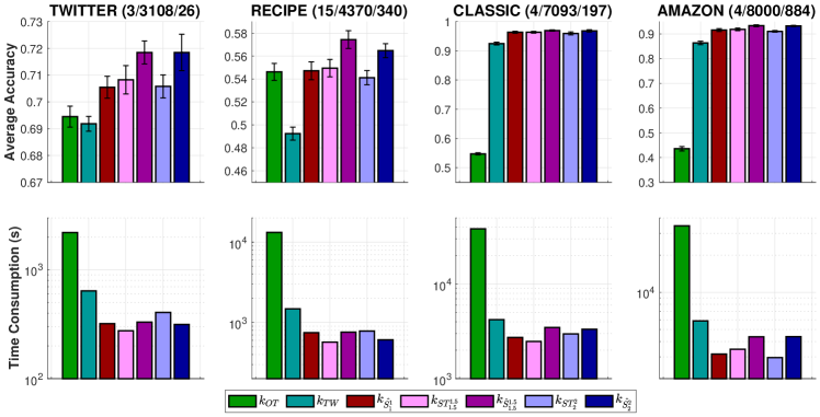
Figure 1: SVM results and time consumption for kernel matrices with graph ${\mathbb{G}}_{\text{Log}}$. For each dataset, the numbers in the parenthesis are the number of classes; the number of documents; and the maximum number of unique words for each document respectively.

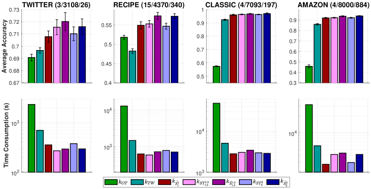
Figure 2: SVM results and time consumption for kernel matrices with graph ${\mathbb{G}}_{\text{Sqrt}}$.

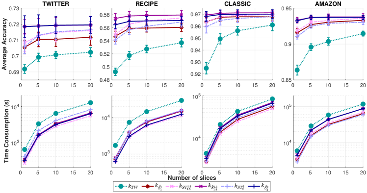
Figure 3: SVM results and time consumption for kernel matrices of slice variants with graph ${\mathbb{G}}_{\text{Log}}$.

Classification. We use kernelized support vector machine (SVM) for document classification and TDA. Specifically, we evaluate regularized Sobolev IPM kernels $k_{\hat{\mathcal{S}}_{1}},k_{\hat{\mathcal{S}}_{1.5}^{1.5}},k_{\hat{\mathcal{S}}_{2}^{2}}$; ST kernels $k_{\mathcal{ST}_{1.5}^{1.5}},k_{\mathcal{ST}_{2}^{2}}$,; and kernels $\exp(-t\bar{d}(\cdot,\cdot))$ with $t>0$, where $\bar{d}$ is a distance (e.g., OT with ground cost $d_{{\mathbb{G}}}$, tree-Wasserstein (TW) with tree sampled from graph ${\mathbb{G}}$) as considered in Le et al. (2022). The kernels corresponding to the two choices of $\bar{d}$ are respectively denoted as $k_{OT},k_{TW}$. Note that kernel $k_{OT}$ is empirically indefinite. We regularize its Gram matrices by adding a sufficiently large diagonal term as in Cuturi (2013).

We randomly split each dataset into $70\%/30\%$ for training and test respectively, with $10$ repeats, and use 1-vs-1 strategy for SVM classification. Typically, hyper-parameters are chosen via cross validation. Concretely, SVM regularization is chosen from $\left\{0.01,0.1,1,10\right\}$, and kernel hyperparameter is chosen from $\{1/q_{s},1/(2q_{s}),1/(5q_{s})\}$ with $s=10,20,\dotsc,90$, where we write $q_{s}$ for the $s\%$ quantile of a subset of corresponding distances on training set. The reported time consumption for kernel matrices includes all preprocessing procedures, e.g., computing shortest paths on graph for $\hat{{\mathcal{S}}}$, $\mathcal{ST}$, or sampling tree from graph for TW.

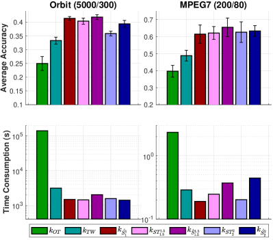
Figure 4: SVM results and time consumption for kernel matrices with graph ${\mathbb{G}}_{\text{Log}}$. For each dataset, the numbers in the parenthesis are respectively the number of PD; and the maximum number of points in PD.

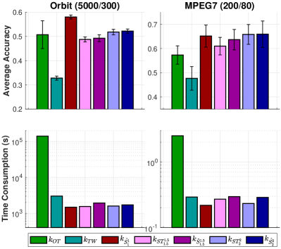
Figure 5: SVM results and time consumption for kernel matrices with graph ${\mathbb{G}}_{\text{Sqrt}}$.

In Table 1, we show the number of pairs requiring to evaluate distance for SVM on each run. Especially, in AMAZON, there are more than $29$ million pairs of probability measures.

SVM results and discussions. The reported results for all datasets are with $M=10^{4}$, except for MPEG7 with $M=10^{3}$ due to the small size of this dataset. We illustrate SVM results and time consumption for kernel matrices on document classification for graphs ${\mathbb{G}}_{\text{Log}}$ and ${\mathbb{G}}_{\text{Sqrt}}$ in Figures 1 and 2 respectively. For TDA, we show the results for ${\mathbb{G}}_{\text{Log}}$ and ${\mathbb{G}}_{\text{Sqrt}}$ in Figures 4 and 5 respectively.

The computation of regularized Sobolev IPM $\hat{{\mathcal{S}}}$ is several-order faster than the traditional OT with ground cost $d_{{\mathbb{G}}}$. Additionally, the computation of $\hat{{\mathcal{S}}}$ is comparable to Sobolev transport $\mathcal{ST}$, a.k.a., a scalable variant of OT on a graph. Especially, for Orbit dataset, either with graph ${\mathbb{G}}_{\text{Log}}$ or ${\mathbb{G}}_{\text{Sqrt}}$, it took more than $39$ hours to evaluate the kernel Gram matrices for the OT kernel $k_{OT}$, but less than $34$ minutes for regularized Sobolev IPM kernels for all exponents $p=1,1.5,2$.

Table 1: The number of pairs of measures on datasets for SVM.

Datasets	#pairs
TWITTER	4394432
RECIPE	8687560
CLASSIC	22890777
AMAZON	29117200
Orbit	11373250
MPEG7	18130

The performances of regularized Sobolev IPM kernels compare favorably with those of ST, OT, TW kernels. Similar to observations in Le et al. (2022), the infiniteness of $k_{OT}$ may become a hinder for its performances in certain applications. For examples, the performances of $k_{OT}$ are affected in most of our experiments, except the ones in RECIPE with graph ${\mathbb{G}}_{\text{Log}}$ and in Orbit with graph ${\mathbb{G}}_{\text{Sqrt}}$. Additionally, TW kernel $k_{TW}$ uses a partial graph information, but is positive definite unlike its counterpart $k_{OT}$. Performances of $k_{TW}$ are worse than its counterpart $k_{OT}$ in RECIPE, but are better than $k_{OT}$ in CLASSIC, AMAZON for both graphs ${\mathbb{G}}_{\text{Log}}$ and ${\mathbb{G}}_{\text{Sqrt}}$, which agrees with observations in Le et al. (2022). For performances, similar to Sobolev transport, one may turn the exponent $p$ for the regularized Sobolev IPM in applications, e.g., via cross validation.

Additionally, we illustrate performance of sliced variants with graph ${\mathbb{G}}_{\text{Log}}$ in Figures 3 and 6 for document classification and TDA respectively. When the number of slices increases, their performances are improved but it comes with a trade-off on increasing the computational time linearly.

Further empirical results are placed in Appendix §C.2.

7 Conclusion

In this work, we propose a novel regularization for Sobolev IPM for probability measures on a graph. The regularized Sobolev IPM admits a closed-form expression for fast computation. It paves the way for applying Sobolev IPM in applications, especially for large-scale settings. For future works, it is interesting to extend the approach to unbalanced setting where input measures may have different total mass, and to go beyond the Sobolev geometric structure, e.g. tackling more challenging geometric structure for IPM such as critic function within a unit ball defined by Besov norm, i.e., Besov IPM, for practical applications.

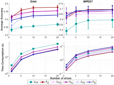
Figure 6: SVM results and time consumption for kernel matrices of slice variants with ${\mathbb{G}}_{\text{Log}}$.

Impact Statement

The paper proposes a novel regularization for Sobolev IPM for probability measures on a graph, which yields a closed form expression for fast computation. Our work paves a way to use Sobolev IPM for practical applications, especially for large-scale settings. To our knowledge, there are no foresee potential societal consequences of our work.

Appendix A Proofs

In this section, we give the detailed proofs for the theoretical results in the main manuscript.

A.1 Proof for Theorem 3.2

Proof.

Let $f\in W_{0}^{1,p}$. We first derive an upper bound for $\left\lVert f\right\rVert_{L^{p}}^{p}$ in terms of $\left\lVert f^{\prime}\right\rVert_{L^{p}_{\hat{w}_{p}}}$. Since $f(z_{0})=0$, we have

$$\left\lVert f\right\rVert_{L^{p}}^{p} =\int_{{\mathbb{G}}}\left|f(x)\right|^{p}\lambda(\mathrm{d}x)$$

$$=\int_{{\mathbb{G}}}\left|f(z_{0})+\int_{[z_{0},x]}f^{\prime}(y)\lambda(\mathrm{d}y)\right|^{p}\lambda(\mathrm{d}x)$$

$$=\int_{{\mathbb{G}}}\left|\int_{{\mathbb{G}}}\mathbf{1}_{[z_{0},x]}(y)f^{\prime}(y)\lambda(\mathrm{d}y)\right|^{p}\lambda(\mathrm{d}x)$$

$$=\lambda({\mathbb{G}})^{p}\int_{{\mathbb{G}}}\left|\frac{1}{\lambda({\mathbb{G}})}\int_{{\mathbb{G}}}\mathbf{1}_{[z_{0},x]}(y)f^{\prime}(y)\lambda(\mathrm{d}y)\right|^{p}\lambda(\mathrm{d}x).$$

Therefore, by applying Jensen’s inequality, we obtain

$$\left\lVert f\right\rVert_{L^{p}}^{p} \leq\lambda({\mathbb{G}})^{p}\int_{{\mathbb{G}}}\left(\frac{1}{\lambda({\mathbb{G}})}\int_{{\mathbb{G}}}\Big{|}\mathbf{1}_{[z_{0},x]}(y)f^{\prime}(y)\Big{|}^{p}\lambda(\mathrm{d}y)\right)\lambda(\mathrm{d}x)$$

$$=\lambda({\mathbb{G}})^{p-1}\int_{{\mathbb{G}}}\int_{{\mathbb{G}}}\Big{|}\mathbf{1}_{[z_{0},x]}(y)f^{\prime}(y)\Big{|}^{p}\lambda(\mathrm{d}y)\lambda(\mathrm{d}x).$$

By Fubini’s theorem, we can interchange the order of the integration. As a consequence, we obtain

$$\left\lVert f\right\rVert_{L^{p}}^{p}\hskip-16.99998pt \leq\lambda({\mathbb{G}})^{p-1}\int_{{\mathbb{G}}}\int_{{\mathbb{G}}}\left|\mathbf{1}_{[z_{0},x]}(y)f^{\prime}(y)\right|^{p}\lambda(\mathrm{d}x)\lambda(\mathrm{d}y)$$ (16)

$$=\lambda({\mathbb{G}})^{p-1}\int_{{\mathbb{G}}}\left(\int_{{\mathbb{G}}}\mathbf{1}_{[z_{0},x]}(y)\lambda(\mathrm{d}x)\right)|f^{\prime}(y)|^{p}\lambda(\mathrm{d}y)$$

$$=\lambda({\mathbb{G}})^{p-1}\int_{{\mathbb{G}}}\left|f^{\prime}(y)\right|^{p}\lambda(\Lambda(y))\lambda(\mathrm{d}y),$$

where we recall that $\Lambda(y):=\left\{x\in{\mathbb{G}}:y\in[z_{0},x]\right\}$ (see Equation (2)). Due to estimate (16), we have

$$\left\lVert f\right\rVert_{W^{1,p}} =\left(\left\lVert f\right\rVert_{L^{p}}^{p}+\left\lVert f^{\prime}\right\rVert_{L^{p}}^{p}\right)^{\frac{1}{p}}$$ (17)

$$\leq\left(\lambda({\mathbb{G}})^{p-1}\int_{{\mathbb{G}}}\left|f^{\prime}(x)\right|^{p}\lambda(\Lambda(x))\lambda(\mathrm{d}x)+\int_{{\mathbb{G}}}|f^{\prime}(x)|^{p}\lambda(\mathrm{d}x)\right)^{\frac{1}{p}}$$

$$=\left(\int_{{\mathbb{G}}}\Big{[}1+\lambda({\mathbb{G}})^{p-1}\lambda(\Lambda(x))\Big{]}|f^{\prime}(x)|^{p}\lambda(\mathrm{d}x)\right)^{\frac{1}{p}}$$

$$\leq\left(\int_{{\mathbb{G}}}\max(1,\lambda({\mathbb{G}})^{p-1})\Big{[}1+\lambda(\Lambda(x))\Big{]}|f^{\prime}(x)|^{p}\lambda(\mathrm{d}x)\right)^{\frac{1}{p}}$$

$$=c_{2}\left\lVert f^{\prime}\right\rVert_{L^{p}_{\hat{w}}},$$

where we recall that $\hat{w}(x):=1+\lambda(\Lambda(x)),\forall x\in{\mathbb{G}}$ (see Equation (5)), and $c_{2}=\left[\max(1,\lambda({\mathbb{G}})^{p-1})\right]^{\frac{1}{p}}$.

We next derive a lower bound for $\left\lVert f\right\rVert_{L^{p}}^{p}$ in terms of $\left\lVert f^{\prime}\right\rVert_{L^{p}_{\hat{w}_{p}}}$ as follows

$$\left\lVert f\right\rVert_{W^{1,p}} =\left(\left\lVert f\right\rVert_{L^{p}}^{p}+\left\lVert f^{\prime}\right\rVert_{L^{p}}^{p}\right)^{\frac{1}{p}}$$ (19)

$$\geq\left\lVert f^{\prime}\right\rVert_{L^{p}}$$

$$=\left(\int_{{\mathbb{G}}}|f^{\prime}(x)|^{p}\lambda(\mathrm{d}x)\right)^{\frac{1}{p}}$$

$$=\left(\int_{{\mathbb{G}}}\frac{1}{1+\lambda({\mathbb{G}})^{p}}\Big{[}1+\lambda({\mathbb{G}})^{p}\Big{]}|f^{\prime}(x)|^{p}\lambda(\mathrm{d}x)\right)^{\frac{1}{p}}$$

$$\geq\left(\int_{{\mathbb{G}}}\frac{1}{1+\lambda({\mathbb{G}})^{p}}\Big{[}1+\lambda({\mathbb{G}})^{p-1}\lambda(\Lambda(x))\Big{]}|f^{\prime}(x)|^{p}\lambda(\mathrm{d}x)\right)^{\frac{1}{p}}$$

$$\geq\left(\int_{{\mathbb{G}}}\frac{\min(1,\lambda({\mathbb{G}})^{p-1})}{1+\lambda({\mathbb{G}})^{p}}\Big{[}1+\lambda(\Lambda(x))\Big{]}|f^{\prime}(x)|^{p}\lambda(\mathrm{d}x)\right)^{\frac{1}{p}}$$

$$=c_{1}\left\lVert f^{\prime}\right\rVert_{L^{p}_{\hat{w}}},$$

where we have used the fact that $\left\lVert f\right\rVert_{L^{p}}\geq 0$ to obtain the inequality (19), and recall that $c_{1}=\left[\frac{\min(1,\lambda({\mathbb{G}})^{p-1})}{1+\lambda({\mathbb{G}})^{p}}\right]^{\frac{1}{p}}$.

Thus, we conclude from Equations (17) and (19) that

$$c_{1}\left\lVert f^{\prime}\right\rVert_{L^{p}_{\hat{w}}}\leq\left\lVert f\right\rVert_{W^{1,p}}\leq c_{2}\left\lVert f^{\prime}\right\rVert_{L^{p}_{\hat{w}}}.$$

The proof is completed.

∎

A.2 Proof for Theorem 3.4

Proof.

Consider a critic function $f\in W_{0}^{1,p^{\prime}}({\mathbb{G}},\lambda)$. Then by Definition 3.1, we have

$$f(x)=f(z_{0})+\int_{[z_{0},x]}f^{\prime}(y)\lambda(\mathrm{d}y)\quad\mbox{for all}\quad x\in{\mathbb{G}}.$$ (20)

Using (20), leveraging the indicator function of the shortest path $[z_{0},x]$, and notice that $\mu({\mathbb{G}})=1$, we get

$$\int_{\mathbb{G}}f(x)\mu(\mathrm{d}x) =\int_{\mathbb{G}}f(z_{0})\mu(\mathrm{d}x)+\int_{\mathbb{G}}\int_{[z_{0},x]}f^{\prime}(y)\lambda(\mathrm{d}y)\mu(\mathrm{d}x)$$

$$=f(z_{0})+\int_{\mathbb{G}}\int_{{\mathbb{G}}}{\bf{1}}_{[z_{0},x]}(y)\,f^{\prime}(y)\lambda(\mathrm{d}y)\mu(\mathrm{d}x).$$

Then, applying Fubini’s theorem to interchange the order of integration in the above last integral, we obtain

$$\int_{\mathbb{G}}f(x)\mu(\mathrm{d}x) =f(z_{0})+\int_{\mathbb{G}}\int_{{\mathbb{G}}}{\bf{1}}_{[z_{0},x]}(y)\,f^{\prime}(y)\mu(\mathrm{d}x)\lambda(\mathrm{d}y)$$

$$=f(z_{0})+\int_{\mathbb{G}}\Big{(}\int_{{\mathbb{G}}}{\bf{1}}_{[z_{0},x]}(y)\,\mu(\mathrm{d}x)\Big{)}f^{\prime}(y)\lambda(\mathrm{d}y).$$

Using the definition of $\Lambda(y)$ in Equation (2), we can rewrite it as

$$\int_{\mathbb{G}}f(x)\mu(\mathrm{d}x)=f(z_{0})+\int_{{\mathbb{G}}}f^{\prime}(y)\mu(\Lambda(y))\,\lambda(\mathrm{d}y).$$

By exactly the same arguments, we also have

$$\int_{\mathbb{G}}f(x)\nu(\mathrm{d}x)=f(z_{0})+\int_{{\mathbb{G}}}f^{\prime}(y)\nu(\Lambda(y))\,\lambda(\mathrm{d}y).$$

Consequently, the regularized Sobolev IPM in Equation (8) can be reformulated as

$$\hat{{\mathcal{S}}}_{p}(\mu,\nu)=\sup_{f\in{\mathcal{B}}(p^{\prime},\hat{w})}\left|\int_{{\mathbb{G}}}f^{\prime}(x)\big{[}\mu(\Lambda(x))-\nu(\Lambda(x))\big{]}\,\lambda(\mathrm{d}x)\right|,$$ (21)

where we recall that ${\mathcal{B}}(p^{\prime},\hat{w}):=\left\{f\in W^{1,p^{\prime}}_{0}:\left\lVert f^{\prime}\right\rVert_{L^{p^{\prime}}_{\hat{w}}}\leq 1\right\}$ (see Equation (7)).

Observe that, we have on one hand

$$\{f^{\prime}:\,f\in{\mathcal{B}}(p^{\prime},\hat{w})\}\subset\{g\in L^{p^{\prime}}({\mathbb{G}},\lambda):\,\|g\|_{L^{p^{\prime}}_{\hat{w}}}\leq 1\}.$$

On the other hand, for any $g\in L^{p^{\prime}}({\mathbb{G}},\lambda)$, we have $g=f^{\prime}$ with $f(x)\coloneqq\int_{[z_{0},x]}g(y)\lambda(\mathrm{d}y)\in L^{p^{\prime}}({\mathbb{G}},\lambda)$.

Therefore, we conclude that

$$\{f^{\prime}:\,f\in{\mathcal{B}}(p^{\prime},\hat{w})\}=\{g\in L^{p^{\prime}}({\mathbb{G}},\lambda):\,\|g\|_{L^{p^{\prime}}_{\hat{w}}}\leq 1\}.$$ (22)

Consequently, if we let $\hat{f}(x):=\frac{\mu(\Lambda(x))-\nu(\Lambda(x))}{\hat{w}(x)}$ for $x\in{\mathbb{G}}$, then Equation (21) can be recasted as

$$\hat{{\mathcal{S}}}_{p}(\mu,\nu) =\sup_{g\in L^{p^{\prime}}({\mathbb{G}},\lambda):\,\left\lVert g\right\rVert_{L^{p^{\prime}}_{\hat{w}}}\leq 1}\left|\int_{{\mathbb{G}}}\hat{w}(x)\hat{f}(x)g(x)\lambda(\mathrm{d}x)\right|$$

$$=\left(\int_{{\mathbb{G}}}\hat{w}(x)|\hat{f}(x)|^{p}\lambda(\mathrm{d}x)\right)^{\frac{1}{p}}$$ (23)

$$=\left(\int_{{\mathbb{G}}}\hat{w}(x)^{1-p}|\mu(\Lambda(x))-\nu(\Lambda(x))|^{p}\lambda(\mathrm{d}x)\right)^{\frac{1}{p}},$$

where Equation (23) is followed by the dual norm of the weighted $L^{p^{\prime}}\!({\mathbb{G}},\lambda)$ with the weighting function $\hat{w}$.

Hence, we have

$$\hat{{\mathcal{S}}}_{p}(\mu,\nu)^{p}=\int_{{\mathbb{G}}}\hat{w}(x)^{1-p}\left|\mu(\Lambda(x))-\nu(\Lambda(x))\right|^{p}\lambda(\mathrm{d}x).$$

The proof is completed. ∎

A.3 Proof for Theorem 3.5

Proof.

We consider the length measure on graph ${\mathbb{G}}$ for $\lambda$. Thus, we have $\lambda(\{x\})=0$ for all $x\in{\mathbb{G}}$.

Consequently, we have

$$\hat{{\mathcal{S}}}_{p}(\mu,\nu)^{p}=\sum_{e=\langle u,v\rangle\in E}\int_{(u,v)}\hat{w}(x)^{1-p}\left|\mu(\Lambda(x))-\nu(\Lambda(x))\right|^{p}\lambda(\mathrm{d}x).$$ (24)

Additionally, we consider input probability measures $\mu,\nu$ supported on nodes in $V$ of graph ${\mathbb{G}}$. Thus, for all edge $e=\langle u,v\rangle\in E$, and any point $x\in(u,v)$, we have

$$\mu(\Lambda(x))-\nu(\Lambda(x))=\mu(\Lambda(x)\setminus(u,v))-\nu(\Lambda(x)\setminus(u,v)).$$

Hence, we can rewrite Equation (24) as

$$\hat{{\mathcal{S}}}_{p}(\mu,\nu)^{p}=\sum_{e=\langle u,v\rangle\in E}\int_{(u,v)}\hat{w}(x)^{1-p}\left|\mu(\Lambda(x)\setminus(u,v))-\nu(\Lambda(x)\setminus(u,v))\right|^{p}\lambda(\mathrm{d}x).$$ (25)

Let us consider edge $e=\langle u,v\rangle\in E$. Then for any $x\in(u,v)$, we have $y\in{\mathbb{G}}\setminus(u,v)$ belongs to $\Lambda(x)$ if and only if $y\in\gamma_{e}$ where we recall that $\Lambda(x)$ and $\gamma_{e}$ are defined in Equation (2). Thus, we have

$$\Lambda(x)\setminus(u,v)=\gamma_{e},\qquad\forall x\in(u,v).$$

Using this fact, we can rewrite Equation (25) as

$$\hat{{\mathcal{S}}}_{p}(\mu,\nu)^{p}=\sum_{e=\langle u,v\rangle\in E}\left|\mu(\gamma_{e})-\nu(\gamma_{e})\right|^{p}\int_{(u,v)}\hat{w}(x)^{1-p}\lambda(\mathrm{d}x).$$ (26)

We next want to compute the integral in (26) for each edge $\langle u,v\rangle\in E$. For this, recall that $\hat{w}(x)=1+\lambda(\Lambda(x))$ (see Equation (5)). Without loss of generality, assume that $d_{{\mathbb{G}}}(z_{0},u)\leq d_{{\mathbb{G}}}(z_{0},v)$, i.e., among two nodes $u,v$ of the edge $e$, node $v$ is farther away from the root node $z_{0}$ than node $u$.

Notice that for $x\in(u,v)$, we can write $x=v+t(u-v)$ for $t\in(0,1)$. With this change of variable, we have

$$\int_{(u,v)}\left[1+\lambda(\Lambda(x))\right]^{1-p}\lambda(\mathrm{d}x)=\int_{0}^{1}\left[1+\lambda(\Lambda(v+t(u-v)))\right]^{1-p}w_{e}\mathrm{d}t$$

Moreover, we have

$$\lambda(\Lambda(v+t(u-v)))=\lambda(\Lambda(v))+\lambda([v,v+t(u-v)])=\lambda(\gamma_{e})+w_{e}t.$$

Therefore,

$$\int_{(u,v)}\left[1+\lambda(\Lambda(x))\right]^{1-p}\lambda(\mathrm{d}x)=\int_{0}^{1}\left[1+\lambda(\gamma_{e})+w_{e}t\right]^{1-p}w_{e}\mathrm{d}t.$$

The last integral can be computed easily depending on the case $p=2$ or $p\neq 2$. As a consequence, we obtain

$$\int_{(u,v)}\left[1+\lambda(\Lambda(x))\right]^{1-p}\lambda(\mathrm{d}x)=\left\{\begin{array}[]{ll}\log{\left(1+\frac{w_{e}}{1+\lambda(\gamma_{e})}\right)}&p=2\\ \frac{\left(1+\lambda(\gamma_{e})+w_{e}\right)^{2-p}-\left(1+\lambda(\gamma_{e})\right)^{2-p}}{2-p}&\text{otherwise.}\end{array}\right.$$

Thus, we have $\int_{(u,v)}\left[1+\lambda(\Lambda(x))\right]^{1-p}\lambda(\mathrm{d}x)=\beta_{e}$ (see Equation (11)). This together with Equation (26) yields

$$\hat{{\mathcal{S}}}_{p}(\mu,\nu)=\left(\sum_{e\in E}\beta_{e}|\mu(\gamma_{e})-\nu(\gamma_{e})|^{p}\right)^{\frac{1}{p}}.$$ (27)

Hence, the proof is completed.

∎

A.4 Proof for Theorem 4.1

Proof.

For $1\leq p\leq\infty$, we will prove that the regularized Sobolev IPM $\hat{{\mathcal{S}}}_{p}(\cdot,\cdot)$ satisfies: (i) nonnegativity, (ii) indiscernibility, (iii) symmetry, and (iv) triangle inequality.

(i) Nonnegativity. By choosing $f=0$ in Definition 3.3, we see that $\hat{{\mathcal{S}}}_{p}(\mu,\nu)\geq 0$ for every measures $(\mu,\nu)$ in ${\mathcal{P}}({\mathbb{G}})\times{\mathcal{P}}({\mathbb{G}})$.

Therefore, the regularized Sobolev IPM $\hat{{\mathcal{S}}}_{p}$ is nonnegative.

(ii) Indiscernibility. Assume that $\hat{{\mathcal{S}}}_{p}(\mu,\nu)=0$. Then we must have

$$\int_{\mathbb{G}}f(x)\mu(\mathrm{d}x)-\int_{\mathbb{G}}f(x)\nu(\mathrm{d}x)=0$$ (28)

for all $f\in W_{0}^{1,p^{\prime}}({\mathbb{G}},\lambda)$ satisfying the constraint $\|f^{\prime}\|_{L^{p^{\prime}}_{\hat{w}}}\leq 1$. Indeed, if by contradiction that (28) is not true, then due to $\hat{{\mathcal{S}}}_{p}(\mu,\nu)=0$ there exists a function $g\in W_{0}^{1,p^{\prime}}({\mathbb{G}},\lambda)$ such that $\|g^{\prime}\|_{L^{p^{\prime}}_{\hat{w}}}\leq 1$, and $\int_{\mathbb{G}}g(x)\mu(\mathrm{d}x)-\int_{\mathbb{G}}g(x)\nu(\mathrm{d}x)<0$. Then, by choosing critic function $f=-g$ in Definition 3.3, we see that $\hat{{\mathcal{S}}}_{p}(\mu,\nu)>0$. This contradicts the assumption $\hat{{\mathcal{S}}}_{p}(\mu,\nu)=0$.

Therefore, Equation (28) holds true. Consequently, we have

$$\int_{\mathbb{G}}f(x)\mu(\mathrm{d}x)=\int_{\mathbb{G}}f(x)\nu(\mathrm{d}x),$$

for every $f\in W_{0}^{1,p^{\prime}}({\mathbb{G}},\lambda)$ with $\|f^{\prime}\|_{L^{p^{\prime}}_{\hat{w}}}\leq 1$. This gives $\mu=\nu$ as desired.

(iii) Symmetry. Observe that if $f\in W_{0}^{1,p^{\prime}}({\mathbb{G}},\lambda)$ with $\|f^{\prime}\|_{L^{p^{\prime}}_{\hat{w}}}\leq 1$, then we have $(-f)\in W_{0}^{1,p^{\prime}}({\mathbb{G}},\lambda)$ with $\|-f^{\prime}\|_{L^{p^{\prime}}_{\hat{w}}}=\|f^{\prime}\|_{L^{p^{\prime}}_{\hat{w}}}\leq 1$. As a consequence, we have

$$\hat{{\mathcal{S}}}_{p}(\mu,\nu)=\hat{{\mathcal{S}}}_{p}(\nu,\mu).$$

(iv) Triangle inequality. Let $\mu,\nu,\sigma$ be probability measures in ${\mathcal{P}}({\mathbb{G}})$. Then, for any critic function $f\in W_{0}^{1,p^{\prime}}({\mathbb{G}},\lambda)$ satisfying $\|f^{\prime}\|_{L^{p^{\prime}}_{\hat{w}}}\leq 1$, we have

$$\left|\int_{\mathbb{G}}f(x)\mu(\mathrm{d}x)-\int_{\mathbb{G}}f(x)\nu(\mathrm{d}x)\right| =\left|\left(\int_{\mathbb{G}}f(x)\mu(\mathrm{d}x)-\int_{\mathbb{G}}f(x)\sigma(\mathrm{d}x)\right)+\left(\int_{\mathbb{G}}f(x)\sigma(\mathrm{d}x)-\int_{\mathbb{G}}f(x)\nu(\mathrm{d}x)\right)\right|$$

$$\leq\left|\int_{\mathbb{G}}f(x)\mu(\mathrm{d}x)-\int_{\mathbb{G}}f(x)\sigma(\mathrm{d}x)\right|+\left|\int_{\mathbb{G}}f(x)\sigma(\mathrm{d}x)-\int_{\mathbb{G}}f(x)\nu(\mathrm{d}x)\right|$$

$$\leq\hat{{\mathcal{S}}}_{p}(\mu,\sigma)+\hat{{\mathcal{S}}}_{p}(\sigma,\nu).$$

By taking the supremum over critic function $f$, this implies that

$$\hat{{\mathcal{S}}}_{p}(\mu,\nu)\leq\hat{{\mathcal{S}}}_{p}(\mu,\sigma)+\hat{{\mathcal{S}}}_{p}(\sigma,\nu).$$

Hence, from these above properties, we conclude that the regularized Sobolev IPM $\hat{{\mathcal{S}}}_{p}(\mu,\nu)$ is a metric for probability measures on the space ${\mathcal{P}}({\mathbb{G}})$.

The proof is completed.

∎

A.5 Proof for Theorem 4.2

Proof.

Given a positive number $c>0$, let us consider ${\mathcal{B}}(p,\hat{w},c):=\left\{f\in W_{0}^{1,p}({\mathbb{G}},\lambda):\left\lVert f^{\prime}\right\rVert_{L^{p}_{\hat{w}}}\leq\frac{1}{c}\right\}$. We define the IPM distance w.r.t. ${\mathcal{B}}(p,\hat{w},c)$ as follows

$$\bar{{\mathcal{S}}}_{p,c}(\mu,\nu):=\sup_{f\in{\mathcal{B}}(p^{\prime},\hat{w},c)}\left|\int_{{\mathbb{G}}}f(x)\mu(\text{d}x)-\int_{{\mathbb{G}}}f(y)\nu(\text{d}y)\right|.$$ (29)

By exploiting the graph structure for the IPM objective function and applying a similar reasoning as in the proof of identity (21) in §A.2, we can rewrite Equation (29) as

$$\bar{{\mathcal{S}}}_{p,c}(\mu,\nu)=\sup_{f\in{\mathcal{B}}(p^{\prime},\hat{w},c)}\left|\int_{{\mathbb{G}}}f^{\prime}(x)\big{[}\mu(\Lambda(x))-\nu(\Lambda(x))\big{]}\,\lambda(\mathrm{d}x)\right|.$$ (30)

Additionally, by using a similar reasoning as in the proof of (22) in §A.2, we have

$$\left\{f^{\prime}:\,f\in{\mathcal{B}}(p^{\prime},\hat{w},c)\right\}=\left\{g\in L^{p^{\prime}}({\mathbb{G}},\lambda):\,\|g\|_{L^{p^{\prime}}_{\hat{w}}}\leq\frac{1}{c}\right\}.$$ (31)

Let $\bar{f}(x):=\frac{\mu(\Lambda(x))-\nu(\Lambda(x))}{c\,\hat{w}(x)}$ for $x\in{\mathbb{G}}$. Then by using (31), Equation (30) can be recasted as

$$\bar{{\mathcal{S}}}_{p,c}(\mu,\nu) =\sup_{g\in L^{p^{\prime}}({\mathbb{G}},\lambda):\,\left\lVert g\right\rVert_{L^{p^{\prime}}_{\hat{w}}}\leq\frac{1}{c}}\left|\int_{{\mathbb{G}}}\hat{w}(x)\bar{f}(x)[c\,g(x)]\lambda(\mathrm{d}x)\right|$$

$$=\sup_{\bar{g}\in L^{p^{\prime}}({\mathbb{G}},\lambda):\,\left\lVert\bar{g}\right\rVert_{L^{p^{\prime}}_{\hat{w}}}\leq 1}\left|\int_{{\mathbb{G}}}\hat{w}(x)\bar{f}(x)\bar{g}(x)\lambda(\mathrm{d}x)\right|$$

$$=\left(\int_{{\mathbb{G}}}\hat{w}(x)|\bar{f}(x)|^{p}\lambda(\mathrm{d}x)\right)^{\frac{1}{p}}$$ (32)

$$=\left(\int_{{\mathbb{G}}}\frac{1}{c^{p}}\hat{w}(x)^{1-p}|\mu(\Lambda(x))-\nu(\Lambda(x))|^{p}\lambda(\mathrm{d}x)\right)^{\frac{1}{p}}$$ (33)

$$=\frac{1}{c}\hat{{\mathcal{S}}}_{p}(\mu,\nu).$$ (34)

where the Equation (32) is followed by the dual norm of the weighted $L^{p^{\prime}}\!({\mathbb{G}},\lambda)$ with weighting function $\hat{w}$; and Equation (34) is followed by the closed-form expression of the regularized Sobolev IPM in Theorem 3.4.

Notice that for $1\leq p<\infty$, from Theorem 3.2, we have

$$c_{1}\left\lVert f^{\prime}\right\rVert_{L^{p^{\prime}}_{\hat{w}}}\leq\left\lVert f\right\rVert_{W^{1,p^{\prime}}}\leq c_{2}\left\lVert f^{\prime}\right\rVert_{L^{p^{\prime}}_{\hat{w}}}.$$

This implies that

$${\mathcal{B}}(p^{\prime},\hat{w},c_{1})\supseteq{\mathcal{B}}(p^{\prime})\supseteq{\mathcal{B}}(p^{\prime},\hat{w},c_{2}).$$

Therefore, for probability measures $\mu,\nu\in{\mathcal{P}}({\mathbb{G}})$, we have

$$\bar{{\mathcal{S}}}_{p,c_{1}}(\mu,\nu)\geq{\mathcal{S}}_{p}(\mu,\nu)\geq\bar{{\mathcal{S}}}_{p,c_{2}}(\mu,\nu).$$ (35)

It follows from Equations (34) and (35) that

$$\frac{1}{c_{1}}\,\hat{{\mathcal{S}}}_{p}(\mu,\nu)\geq{\mathcal{S}}_{p}(\mu,\nu)\geq\frac{1}{c_{2}}\,\hat{{\mathcal{S}}}_{p}(\mu,\nu),$$

which gives

$$c_{1}\,{\mathcal{S}}_{p}(\mu,\nu)\leq\hat{{\mathcal{S}}}_{p}(\mu,\nu)\leq c_{2}\,{\mathcal{S}}_{p}(\mu,\nu).$$

The proof is complete.

∎

A.6 Proof for Proposition 4.3

Proof.

Observe that $0\leq\lambda(\Lambda(x))\leq\lambda({\mathbb{G}})$ for all $x\in{\mathbb{G}}$. Consequently, we have

$$\frac{1}{1+\lambda({{\mathbb{G}}})}(1+\lambda(\Lambda(x)))\leq 1\leq 1+\lambda(\Lambda(x)),\quad\forall x\in{\mathbb{G}}.$$

Therefore, for $1\leq p<\infty$, we have

$$(1+\lambda({{\mathbb{G}}}))^{p-1}\hat{w}(x)^{1-p}\geq 1\geq\hat{w}(x)^{1-p},\quad\forall x\in{\mathbb{G}}.$$ (36)

Additionally, recall that the Sobolev transport $\mathcal{ST}_{\!p}$ for $\mu,\nu\in{\mathcal{P}}({\mathbb{G}})$ admits a closed-form expression (Le et al., 2022, Proposition 3.5)

$$\mathcal{ST}_{\!p}(\mu,\nu)=\left(\int_{{\mathbb{G}}}\left|\mu(\Lambda(x))-\nu(\Lambda(x))\right|^{p}\lambda(\mathrm{d}x)\right)^{\frac{1}{p}}.$$ (37)

By combining the closed-form expression of the regularized Sobolev IPM (Equation (9) in Theorem 3.4) with Equations (36) and (37), we obtain

$$\hat{{\mathcal{S}}}_{p}(\mu,\nu)\leq\mathcal{ST}_{\!p}(\mu,\nu)\leq(1+\lambda({{\mathbb{G}}}))^{\frac{p-1}{p}}\hat{{\mathcal{S}}}_{p}(\mu,\nu).$$

It follows that

$$(1+\lambda({{\mathbb{G}}}))^{\frac{1-p}{p}}\mathcal{ST}_{\!p}(\mu,\nu)\leq\hat{{\mathcal{S}}}_{p}(\mu,\nu)\leq\mathcal{ST}_{\!p}(\mu,\nu).$$ (38)

The proof is complete.

∎

A.7 Proof for Proposition 4.4

Proof.

For convenience, let $\bar{h}(x):=\mu(\Lambda(x))-\nu(\Lambda(x))$. Recall also that $p^{\prime}=\frac{p}{p-1}$ and $q^{\prime}=\frac{q}{q-1}$ are respectively the conjugate of $p$ and $q$. Then it follows from Theorem 3.4 that

$$\hat{{\mathcal{S}}}_{p}(\mu,\nu)^{p}=\int_{{\mathbb{G}}}\hskip-3.00003pt\hat{w}(x)^{1-p}|\bar{h}(x)|^{p}\lambda(\mathrm{d}x)=\int_{{\mathbb{G}}}\hskip-3.00003pt\left(\hat{w}(x)^{\frac{q-p}{q}}\right)\left(\hat{w}(x)^{\frac{p(1-q)}{q}}|\bar{h}(x)|^{p}\right)\lambda(\mathrm{d}x).$$

We can apply Hölder inequality with $l=\frac{q}{p}>1$ and $l^{\prime}=\frac{q}{q-p}$ to obtain

$$\hat{{\mathcal{S}}}_{p}(\mu,\nu)^{p} \leq\left[\int_{{\mathbb{G}}}\hskip-3.00003pt\left(\hat{w}(x)^{\frac{q-p}{q}}\right)^{\frac{q}{q-p}}\lambda(\mathrm{d}x)\right]^{\frac{q-p}{q}}\left[\int_{{\mathbb{G}}}\hskip-3.00003pt\left(\hat{w}(x)^{\frac{p(1-q)}{q}}|\bar{h}(x)|^{p}\right)^{\frac{q}{p}}\lambda(\mathrm{d}x)\right]^{\frac{p}{q}}$$

$$=\left[\int_{{\mathbb{G}}}\hskip-3.00003pt\hat{w}(x)\lambda(\mathrm{d}x)\right]^{\frac{q-p}{q}}\left[\int_{{\mathbb{G}}}\hskip-3.00003pt\hat{w}(x)^{1-q}|\bar{h}(x)|^{q}\lambda(\mathrm{d}x)\right]^{\frac{p}{q}}.$$

In addition, it follow directly from the definition in Equation (5) that

$$\hat{w}(x)\leq 1+\lambda({\mathbb{G}}).$$

for every $x\in{\mathbb{G}}$. Therefore, we further deduce from above estimate and Theorem 3.4 that

$$\hat{{\mathcal{S}}}_{p}(\mu,\nu)^{p} \leq\left[\int_{{\mathbb{G}}}\hskip-3.00003pt\left(1+\lambda({\mathbb{G}})\right)\lambda(\mathrm{d}x)\right]^{\frac{q-p}{q}}\left[\int_{{\mathbb{G}}}\hskip-3.00003pt\hat{w}(x)^{1-q}|\bar{h}(x)|^{q}\lambda(\mathrm{d}x)\right]^{\frac{p}{q}}$$

$$=\left[\lambda({\mathbb{G}})\left(1+\lambda({\mathbb{G}})\right)\right]^{\frac{q-p}{q}}\hat{{\mathcal{S}}}_{q}(\mu,\nu)^{p}.$$

Hence, we obtain

$$\hat{{\mathcal{S}}}_{p}(\mu,\nu)\leq\left[\lambda({\mathbb{G}})\left(1+\lambda({\mathbb{G}})\right)\right]^{\frac{1}{p}-\frac{1}{q}}\hat{{\mathcal{S}}}_{q}(\mu,\nu).$$

This completes the proof of the proposition. ∎

A.8 Proof for Proposition 4.5

Proof.

From Proposition 4.3, we have

$$\hat{{\mathcal{S}}}_{1}(\mu,\nu)=\mathcal{ST}_{\!1}(\mu,\nu).$$

Additionally, following Le et al. (2022, Corollary 4.3), when graph ${\mathbb{G}}$ is a tree and $\lambda$ is the length measure on ${\mathbb{G}}$, we have

$$\mathcal{ST}_{\!1}(\mu,\nu)={\mathcal{W}}_{1}(\mu,\nu),$$

where the $1$-Wasserstein distance ${\mathcal{W}}_{1}$ is defined w.r.t. the ground cost $d_{{\mathbb{G}}}$.

Hence, we obtain

$$\hat{{\mathcal{S}}}_{1}(\mu,\nu)={\mathcal{W}}_{1}(\mu,\nu).$$

The proof is complete. ∎

A.9 Proof for Proposition 4.6

Proof.

From Proposition 4.5, we have

$$\hat{{\mathcal{S}}}_{1}(\mu,\nu)={\mathcal{W}}_{1}(\mu,\nu).$$

Additionally, Proposition 4.4 gives

$$\hat{{\mathcal{S}}}_{1}(\mu,\nu)\leq\left[\lambda({\mathbb{G}})(1+\lambda({\mathbb{G}}))\right]^{\frac{p-1}{p}}\hat{\mathcal{S}}_{p}(\mu,\nu).$$

Therefore, we obtain

$${\mathcal{W}}_{1}(\mu,\nu)\leq\left[\lambda({\mathbb{G}})(1+\lambda({\mathbb{G}}))\right]^{\frac{p-1}{p}}\hat{\mathcal{S}}_{p}(\mu,\nu).$$

It then follows that

$$\hat{\mathcal{S}}_{p}(\mu,\nu)\geq\left[\lambda({\mathbb{G}})(1+\lambda({\mathbb{G}}))\right]^{\frac{1-p}{p}}{\mathcal{W}}_{1}(\mu,\nu).$$

The proof is complete.

∎

A.10 Proof for Proposition 4.7

Proof.

For $x,z\in\mathbb{R}^{m}$, consider the following function

$$\ell_{p}(x,z)=\left\lVert x-z\right\rVert_{p}=\left(\sum_{i=1}^{m}\left|x_{(i)}-z_{(i)}\right|^{p}\right)^{1/p},$$

where $x_{(i)}$ is the $i^{th}$ coordinate of $x$. We will prove that for $1\leq p\leq 2$, the functions $\ell_{p}$ and $\ell_{p}^{p}$ are negative definite.

For $a,b\in\mathbb{R}$, it is obvious that the function $(a,b)\mapsto(a-b)^{2}$ is negative definite. For $1\leq p\leq 2$, following Berg et al. (1984, Corollary 2.10, pp.78), the function $(a,b)\mapsto|a-b|^{p}$ is also negative definite.

Consequently, the function $\ell_{p}^{p}$ is negative definite since it is a sum of negative definite functions. Moreover, following Berg et al. (1984, Corollary 2.10, pp.78), we also have that the function $\ell_{p}$ is negative definite.

Let $m$ be the number of edges in the graph ${\mathbb{G}}$, i.e., $|E|=m$. Following Theorem 3.5, we regard $({\beta}_{e})^{\frac{1}{p}}\mu(\gamma_{e})$ for each edge $e\in E$ of graph ${\mathbb{G}}$ as a feature map for probability measure $\mu$ onto $\mathbb{R}^{m}_{+}$. Therefore, $\hat{{\mathcal{S}}}_{p}$ is equal to the function $\ell_{p}$ between these feature maps.

Hence, $\hat{{\mathcal{S}}}_{p}$ and $\hat{{\mathcal{S}}}_{p}^{p}$ are negative definite for $1\leq p\leq 2$. The proof is complete. ∎

A.11 Proof for Proposition 4.8

Proof.

For probability measures $\mu,\nu$ supported on nodes in $V$ of graph ${\mathbb{G}}$, $1\leq p\leq 2$, and an integer $\tau\in\mathbb{N}^{*}$, we define the following kernels

$$k_{\hat{{\mathcal{S}}}_{p}}^{\tau}(\mu,\nu):=\exp\left(-t\frac{\hat{{\mathcal{S}}}_{p}(\mu,\nu)}{\tau}\right),$$ (39)

$$k_{\hat{{\mathcal{S}}}_{p}^{p}}^{\tau}(\mu,\nu):=\exp\left(-t\frac{\hat{{\mathcal{S}}}_{p}(\mu,\nu)^{p}}{\tau}\right).$$ (40)

Observe that $k_{\hat{{\mathcal{S}}}_{p}}^{\tau}(\mu,\nu)^{\tau}=k_{\hat{{\mathcal{S}}}_{p}}(\mu,\nu)$ and $k_{\hat{{\mathcal{S}}}_{p}^{p}}^{\tau}(\mu,\nu)^{\tau}=k_{\hat{{\mathcal{S}}}_{p}^{p}}(\mu,\nu)$.

Furthermore, both kernels $k_{\hat{{\mathcal{S}}}_{p}}^{\tau}$ and $k_{\hat{{\mathcal{S}}}_{p}^{p}}^{\tau}$ are positive definite.

Hence, following Berg et al. (1984, §3, Definition 2.6, pp. 76), the kernels $k_{\hat{\mathcal{S}}_{p}}$ and $k_{\hat{\mathcal{S}}^{p}_{p}}$ are infinitely divisible. The proof is complete.

∎

Appendix B Reviews

In this section, we give a review for related notions used in the development of our proposed approach.

B.1 A Review on Functional Spaces

We give a review on the $L^{p}$ space, the weighted $L^{p}$ space, and Sobolev norm including the case the exponent $p=\infty$.

$L^{p}$ space.

For a nonnegative Borel measure $\lambda$ on ${\mathbb{G}}$, denote $L^{p}({\mathbb{G}},\lambda)$ as the space of all Borel measurable functions $f:{\mathbb{G}}\to\mathbb{R}$ such that $\int_{\mathbb{G}}|f(y)|^{p}\lambda(\mathrm{d}y)<\infty$. For $p=\infty$, we instead assume that $f$ is bounded $\lambda$-a.e. Functions $f_{1},f_{2}\in L^{p}({\mathbb{G}},\lambda)$ are considered to be the same if $f_{1}(x)=f_{2}(x)$ for $\lambda$-a.e. $x\in{\mathbb{G}}$.

Then, $L^{p}({\mathbb{G}},\lambda)$ is a normed space with the norm defined by

$$\|f\|_{L^{p}}:=\left(\int_{\mathbb{G}}|f(y)|^{p}\lambda(\mathrm{d}y)\right)^{\frac{1}{p}}\text{ for }1\leq p<\infty.$$

On the other hand, for $p=\infty$ we have

$$\|f\|_{L^{\infty}}:=\inf\left\{t\in\mathbb{R}:\,|f(x)|\leq t\mbox{ for $\lambda$-a.e. }x\in{\mathbb{G}}\right\}.$$

${L^{p}_{\hat{w}}}$ space.

For a nonnegative Borel measure $\lambda$ on ${\mathbb{G}}$, and a positive weight function $\hat{w}$ on $G$, i.e., $\hat{w}(x)>0,\forall x\in{\mathbb{G}}$, denote $L^{p}_{\hat{w}}({\mathbb{G}},\lambda)$ as the space of all Borel measurable functions $f:{\mathbb{G}}\to\mathbb{R}$ such that $\int_{\mathbb{G}}\hat{w}(x)|f(x)|^{p}\lambda(\mathrm{d}x)<\infty$. For $p=\infty$, we instead assume that $f$ is bounded $\hat{w}\lambda$-a.e. Then, $L^{p}_{\hat{w}}({\mathbb{G}},\lambda)$ is a normed space with the norm defined by

$$\|f\|_{L^{p}_{\hat{w}}}:=\left(\int_{\mathbb{G}}\hat{w}(x)|f(x)|^{p}\lambda(\mathrm{d}x)\right)^{\frac{1}{p}}\text{ for }1\leq p<\infty.$$

For the case $p=\infty$, as $\hat{w}(x)>0$ for every $x\in{\mathbb{G}}$ we have

$$\|f\|_{L^{\infty}_{\hat{w}}} :=\inf\left\{t\in\mathbb{R}:\,|f(x)|\leq t\mbox{ for $(\hat{w}\lambda)$-a.e. }x\in{\mathbb{G}}\right\}$$

$$=\inf\left\{t\in\mathbb{R}:\,|f(x)|\leq t\mbox{ for $\lambda$-a.e. }x\in{\mathbb{G}}\right\}$$

$$=\|f\|_{L^{\infty}}.$$

Sobolev norm.

For $1\leq p\leq\infty$ and a function $f\in W^{1,p}({\mathbb{G}},\lambda)$, its Sobolev norm (Adams & Fournier, 2003, §3.1) is

$$\left\lVert f\right\rVert_{W^{1,p}}=\left(\left\lVert f\right\rVert_{p}^{p}+\left\lVert f^{\prime}\right\rVert_{p}^{p}\right)^{\frac{1}{p}}.$$ (41)

When $p=\infty$, its norm is defined as follows:

$$\left\lVert f\right\rVert_{W^{1,\infty}}=\left\lVert f\right\rVert_{\infty}+\left\lVert f^{\prime}\right\rVert_{\infty}.$$ (42)

B.2 A Review on Sobolev Transport

We give a review on the Sobolev transport for probability measures on a graph, and the length measure on a graph.

Sobolev transport. For $\mu,\nu\in{\mathcal{P}}({\mathbb{G}})$, and $1\leq p\leq\infty$, the $p$-order Sobolev transport (ST) (Le et al., 2022, Definition 3.2) is defined as

$$\mathcal{ST}_{p}(\mu,\nu)\coloneqq\left\{\begin{array}[]{cl}\sup\Big{[}\int_{\mathbb{G}}f(x)\mu(\mathrm{d}x)-\int_{\mathbb{G}}f(x)\nu(\mathrm{d}x)\Big{]}\\ \hskip 8.00003pt\mathrm{s.t.}\,f\in W^{1,p^{\prime}}\hskip-3.00003pt({\mathbb{G}},\lambda),\,\|f^{\prime}\|_{L^{p^{\prime}}({\mathbb{G}},\lambda)}\leq 1,\end{array}\right.$$ (43)

where we write $f^{\prime}$ for the generalized graph derivative of $f$, and $W^{1,p^{\prime}}\hskip-3.00003pt({\mathbb{G}},\lambda)$ for the graph-based Sobolev space on ${\mathbb{G}}$.

Proposition B.1 (Closed-form expression of Sobolev transport (Le et al., 2022)).

Let $\lambda$ be any nonnegative Borel measure on ${\mathbb{G}}$, and let $1\leq p<\infty$. Then, we have

$$\mathcal{ST}_{p}(\mu,\nu)=\left(\int_{{\mathbb{G}}}|\mu(\Lambda(x))-\nu(\Lambda(x))|^{p}\,\lambda(\mathrm{d}x)\right)^{\frac{1}{p}},$$

where $\Lambda(x)$ is the subset of ${\mathbb{G}}$ defined by Equation (2).

Definition B.2 (Length measure (Le et al., 2022)).

Let $\lambda^{*}$ be the unique Borel measure on ${\mathbb{G}}$ such that the restriction of $\lambda^{*}$ on any edge is the length measure of that edge. That is, $\lambda^{*}$ satisfies:

1. For any edge $e$ connecting two nodes $u$ and $v$, we have $\lambda^{*}(\langle x,y\rangle)=(t-s)w_{e}$ whenever $x=(1-s)u+sv$ and $y=(1-t)u+tv$ for $s,t\in[0,1)$ with $s\leq t$. Here, recall that $\langle x,y\rangle$ is the line segment in $e$ connecting $x$ and $y$.

2. For any Borel set $F\subset{\mathbb{G}}$, we have

   $$\lambda^{*}(F)=\sum_{e\in E}\lambda^{*}(F\cap e).$$

Lemma B.3 ($\lambda^{*}$ is the length measure on graph (Le et al., 2022)).

Suppose that ${\mathbb{G}}$ has no short cuts, namely, any edge $e$ is a shortest path connecting its two end-points. Then, $\lambda^{*}$ is a length measure in the sense that

$$\lambda^{*}([x,y])=d_{\mathbb{G}}(x,y)$$

for any shortest path $[x,y]$ connecting $x,y$. Particularly, $\lambda^{*}$ has no atom in the sense that $\lambda^{*}(\{x\})=0$ for every $x\in{\mathbb{G}}$.

B.3 A Review on IPM and Wasserstein Distance

We give a review on IPM and Wasserstein distance for probability measures.

IPM.

Integral probability metrics (IPM) for probability measures $\mu,\nu$ are defined as follows:

$$\gamma_{{\mathcal{F}}}(\mu,\nu)=\sup_{f\in{\mathcal{F}}}\left|\int_{\Omega}f(x)\mu(\text{d}x)-\int_{\Omega}f(y)\nu(\text{d}y)\right|.$$ (44)

Special case: $1$-Wasserstein distance (dual formulation).

The $1$-Wasserstein distance is a special case of IPM. In particular, for ${\mathcal{F}}={\mathcal{F}}_{W}:=\left\{f:\left|f(x)-f(y)\right|\leq d_{{\mathbb{G}}}(x,y)\right\}$ where recall that $d_{{\mathbb{G}}}$ is the graph metric on graph ${\mathbb{G}}$, then IPM is equal to the $1$-Wasserstein distance with ground cost $d_{{\mathbb{G}}}$

$${\mathcal{W}}(\mu,\nu)=\sup_{f\in{\mathcal{F}}_{W}}\left|\int_{{\mathbb{G}}}f(x)\mu(\text{d}x)-\int_{{\mathbb{G}}}f(y)\nu(\text{d}y)\right|.$$ (45)

Besides Sobolev IPM, and $1$-Wasserstein distance, some other popular instances of IPM include: (i) Besov IPM, (ii) Dudley metric, (iii) total variation metric, (iv) Kolmogorov metric, (v) maximum mean discrepancies (MMD) (Müller, 1997; Sriperumbudur et al., 2009).

$p$-Wasserstein distance (primal formulation).

Let $1\leq p<\infty$, suppose that $\mu$ and $\nu$ are two nonnegative Borel measures on ${\mathbb{G}}$ satisfying $\mu({\mathbb{G}})=\nu({\mathbb{G}})=1$. Then, the $p$-Wasserstein distance between $\mu$ and $\nu$ is defined as follows:

$${\mathcal{W}}_{p}(\mu,\nu)^{p} =\inf_{\pi\in\Pi(\mu,\nu)}\int_{{\mathbb{G}}\times{\mathbb{G}}}d_{\mathbb{G}}(x,y)^{p}\pi(\mathrm{d}x,\mathrm{d}y),$$

where $\Pi(\mu,\nu):=\Big{\{}\pi\in{\mathcal{P}}({\mathbb{G}}\times{\mathbb{G}}):\,\pi_{1}=\mu,\,\pi_{2}=\nu\Big{\}}$; $\pi_{1},\pi_{2}$ are the first and second marginals of $\pi$ respectively.

B.4 A Review on Kernels

We review definitions and theorems about kernels used in our work.

Positive Definite Kernels (Berg et al., 1984, pp. 66–67).

A kernel function $k:\Omega\times\Omega\rightarrow\mathbb{R}$ is positive definite if for every positive integer $m\geq 2$ and every points $x_{1},x_{2},...,x_{m}\in\Omega$, we have

$$\sum_{i,j=1}^{m}c_{i}c_{j}k(x_{i},x_{j})\geq 0\qquad\forall c_{1},...,c_{m}\in\mathbb{R}.$$

Negative Definite Kernels (Berg et al., 1984, pp. 66–67).

A kernel function $k:\Omega\times\Omega\rightarrow\mathbb{R}$ is negative definite if for every integer $m\geq 2$ and every points $x_{1},x_{2},...,x_{m}\in\Omega$, we have

$$\sum_{i,j=1}^{m}c_{i}c_{j}k(x_{i},x_{j})\leq 0,\qquad\quad\forall c_{1},...,c_{m}\in\mathbb{R}\,\,\text{ s.t. }\,\sum_{i=1}^{m}c_{i}=0.$$

Theorem 3.2.2 in Berg et al. (1984, pp. 74).

Let $\bar{k}$ be a negative definite kernel function. Then, for every $t>0$, the kernel

$$k(x,z)\triangleq\exp{\left(-t\bar{k}(x,z)\right)}$$

is positive definite.

Definition 2.6 in Berg et al. (1984, pp. 76).

A positive definite kernel $\bar{k}$ is infinitely divisible if for each $n\in{\mathbb{N}}^{*}$, there exists a positive definite kernel $\bar{k}_{n}$ such that

$$\bar{k}=(\bar{k}_{n})^{n}.$$

Corollary 2.10 in Berg et al. (1984, pp. 78).

Let $\bar{k}$ be a negative definite kernel function. Then, for $0<t<1$, the kernel

$$k(x,z)\triangleq\left[\bar{k}(x,z)\right]^{t}$$

is negative definite.

B.5 Persistence Diagrams

We refer the readers to Kusano et al. (2017, §2) for the review on mathematical framework for persistence diagrams (e.g., persistence diagrams, filtrations, persistent homology).

Appendix C Further Results and Discussions

In this section, we give further experimental results and further discussions for the regularized Sobolev IPM.

C.1 Further Results

For the case $p=\infty$.

The closed-form expression of regularized Sobolev IPM for $p=\infty$ is

$$\hat{{\mathcal{S}}}_{\infty}(\mu,\nu)=\inf\left\{t\in\mathcal{R}:\left|\frac{\mu(\Lambda(x))-\nu(\Lambda(x))}{\hat{w}(x)}\right|\leq t\mbox{ for $(\hat{w}\lambda)$-a.e. }x\in{\mathbb{G}}\right\}.$$

Proof.

We follow the same reasoning for the proof of Theorem 3.4. We recall Equation (LABEL:app:eq:dualnorm_regSobolevIPM)

$$\hat{{\mathcal{S}}}_{p}(\mu,\nu)=\sup_{\left\lVert g\right\rVert_{L^{p^{\prime}}_{\hat{w}}}\leq 1}~\int_{{\mathbb{G}}}\hat{w}(x)\hat{f}(x)g(x)\lambda(\mathrm{d}x).$$ (46)

Therefore, for $p=\infty$, by using the dual norm, and let $\hat{f}(x):=\frac{\mu(\Lambda(x))-\nu(\Lambda(x))}{\hat{w}(x)}$, for all $x\in{\mathbb{G}}$, we have

$$\hat{{\mathcal{S}}}_{\infty}(\mu,\nu)=\left\lVert\hat{f}(x)\right\rVert_{L^{\infty}_{\hat{w}}},$$ (47)

which is the weighted $L^{\infty}({\mathbb{G}},\lambda)$-norm with the weighting function $\hat{w}$.

Hence, we obtain

$$\hat{{\mathcal{S}}}_{\infty}(\mu,\nu)=\inf\left\{t\in\mathcal{R}:\left|\frac{\mu(\Lambda(x))-\nu(\Lambda(x))}{\hat{w}(x)}\right|\leq t\mbox{ for $(\hat{w}\lambda)$-a.e. }x\in{\mathbb{G}}\right\}.$$

The proof is completed. ∎

C.2 Further Experimental Results

We present further results for the regularized Sobolev IPM for document classification and TDA for both graphs ${\mathbb{G}}_{\text{Sqrt}}$ and ${\mathbb{G}}_{\text{Log}}$ with different numbers of nodes $M$.

+ For document classification.

• Figures 7 and 8 illustrate SVM results and time consumption for kernel matrices on graphs ${\mathbb{G}}_{\text{Sqrt}}$ and ${\mathbb{G}}_{\text{Log}}$ respectively where the number of nodes $M=1000$.

• Figures 9 and 10 illustrate SVM results and time consumption for kernel matrices on graphs ${\mathbb{G}}_{\text{Sqrt}}$ and ${\mathbb{G}}_{\text{Log}}$ respectively where the number of nodes $M=100$.

+ For TDA.

• Figures 11 and 12 illustrate SVM results and time consumption for kernel matrices on graphs ${\mathbb{G}}_{\text{Sqrt}}$ and ${\mathbb{G}}_{\text{Log}}$ respectively where the number of nodes $M=1000$.

• Figures 13 and 14 illustrate SVM results and time consumption for kernel matrices on graphs ${\mathbb{G}}_{\text{Sqrt}}$ and ${\mathbb{G}}_{\text{Log}}$ respectively where the number of nodes $M=100$.

We next provide further results for the regularized Sobolev IPM when varying the number of slices on both graphs ${\mathbb{G}}_{\text{Sqrt}}$ and ${\mathbb{G}}_{\text{Log}}$ for document classification and TDA.

+ For document classification.

• Figure 15 illustrates SVM results and time consumption for kernel matrices on graph ${\mathbb{G}}_{\text{Sqrt}}$ where the number of nodes $M=10^{4}$.

• Figures 16 and 17 illustrate SVM results and time consumption for kernel matrices on graphs ${\mathbb{G}}_{\text{Sqrt}}$ and ${\mathbb{G}}_{\text{Log}}$ respectively where the number of nodes $M=1000$.

• Figures 18 and 19 illustrate SVM results and time consumption for kernel matrices on graphs ${\mathbb{G}}_{\text{Sqrt}}$ and ${\mathbb{G}}_{\text{Log}}$ respectively where the number of nodes $M=100$.

+ For TDA.

• Figure 20 illustrates SVM results and time consumption for kernel matrices on graph ${\mathbb{G}}_{\text{Sqrt}}$ where the number of nodes $M=10^{4}$ for Orbit and $M=10^{3}$ for MPEG7.

• Figures 21(a) and 22(a) illustrate SVM results and time consumption for kernel matrices on graphs ${\mathbb{G}}_{\text{Sqrt}}$ and ${\mathbb{G}}_{\text{Log}}$ respectively where the number of nodes $M=1000$.

• Figures 21(b) and 22(b) illustrate SVM results and time consumption for kernel matrices on graphs ${\mathbb{G}}_{\text{Sqrt}}$ and ${\mathbb{G}}_{\text{Log}}$ respectively where the number of nodes $M=100$.

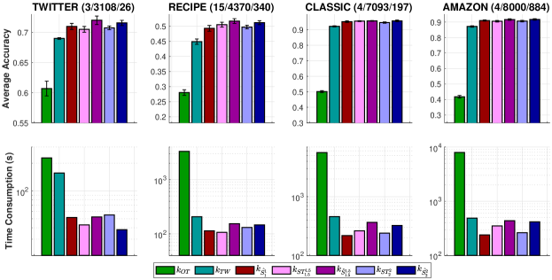
Figure 7: SVM results and time consumption for kernel matrices in document classification with graph ${\mathbb{G}}_{\text{Sqrt}}$ where the number of nodes $M=1000$.

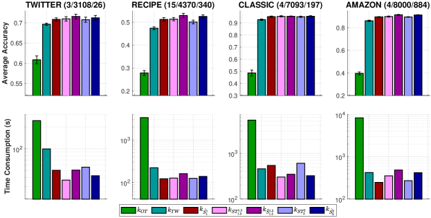
Figure 8: SVM results and time consumption for kernel matrices in document classification with graph ${\mathbb{G}}_{\text{Log}}$ where the number of nodes $M=1000$.

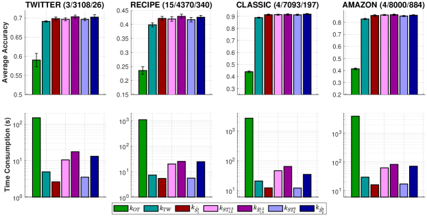
Figure 9: SVM results and time consumption for kernel matrices in document classification with graph ${\mathbb{G}}_{\text{Sqrt}}$ where the number of nodes $M=100$.

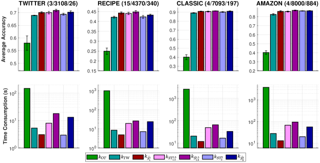
Figure 10: SVM results and time consumption for kernel matrices in document classification with graph ${\mathbb{G}}_{\text{Log}}$ where the number of nodes $M=100$.

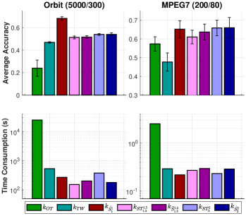
Figure 11: SVM results and time consumption for kernel matrices in TDA with graph ${\mathbb{G}}_{\text{Sqrt}}$ where the number of nodes $M=1000$.

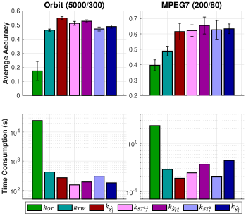
Figure 12: SVM results and time consumption for kernel matrices in TDA with graph ${\mathbb{G}}_{\text{Log}}$ where the number of nodes $M=1000$.

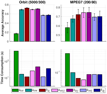
Figure 13: SVM results and time consumption for kernel matrices in TDA with graph ${\mathbb{G}}_{\text{Sqrt}}$ where the number of nodes $M=100$.

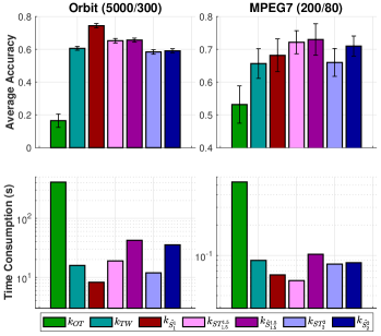
Figure 14: SVM results and time consumption for kernel matrices in TDA with graph ${\mathbb{G}}_{\text{Log}}$ where the number of nodes $M=100$.

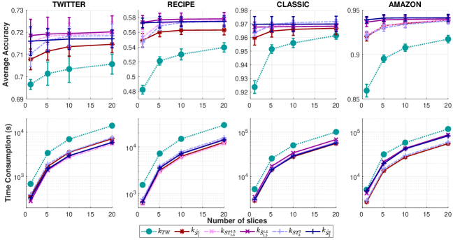
Figure 15: SVM results and time consumption for kernel matrices of slice variants with graph ${\mathbb{G}}_{\text{Sqrt}}$ where the number of nodes $M=10^{4}$.

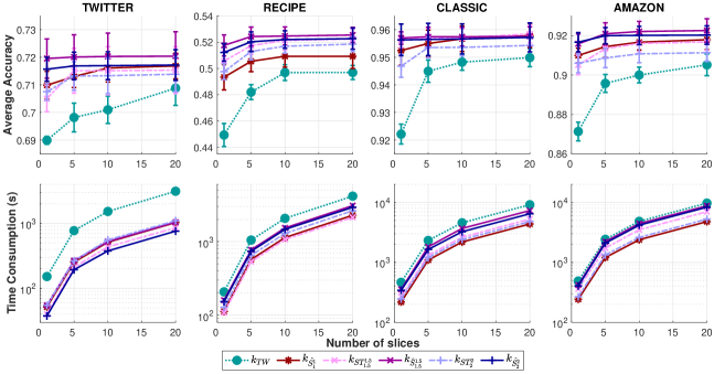
Figure 16: SVM results and time consumption for kernel matrices of slice variants with graph ${\mathbb{G}}_{\text{Sqrt}}$ where the number of nodes $M=1000$.

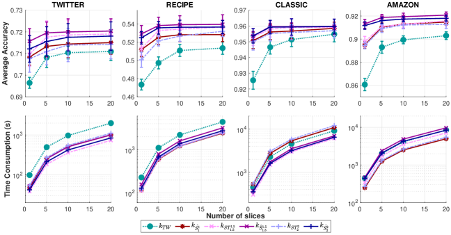
Figure 17: SVM results and time consumption for kernel matrices of slice variants with graph ${\mathbb{G}}_{\text{Log}}$ where the number of nodes $M=1000$.

Figure 18: SVM results and time consumption for kernel matrices of slice variants with graph ${\mathbb{G}}_{\text{Sqrt}}$ where the number of nodes $M=100$.

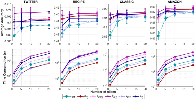
Figure 19: SVM results and time consumption for kernel matrices of slice variants with graph ${\mathbb{G}}_{\text{Log}}$ where the number of nodes $M=100$.

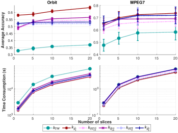
Figure 20: SVM results and time consumption for kernel matrices of slice variants with graph ${\mathbb{G}}_{\text{Sqrt}}$ where the number of nodes $M=10^{4}$ for Orbit, and $M=10^{3}$ for MPEG7.

(a) With $M=1000$.

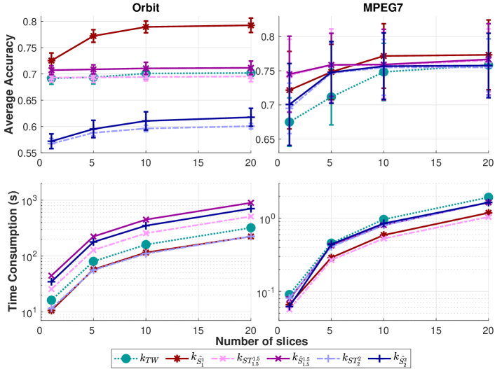
(b) With $M=100$.

Figure 21: SVM results and time consumption for kernel matrices of slice variants with graph ${\mathbb{G}}_{\text{Sqrt}}$.

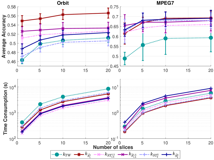
(a) With $M=1000$.

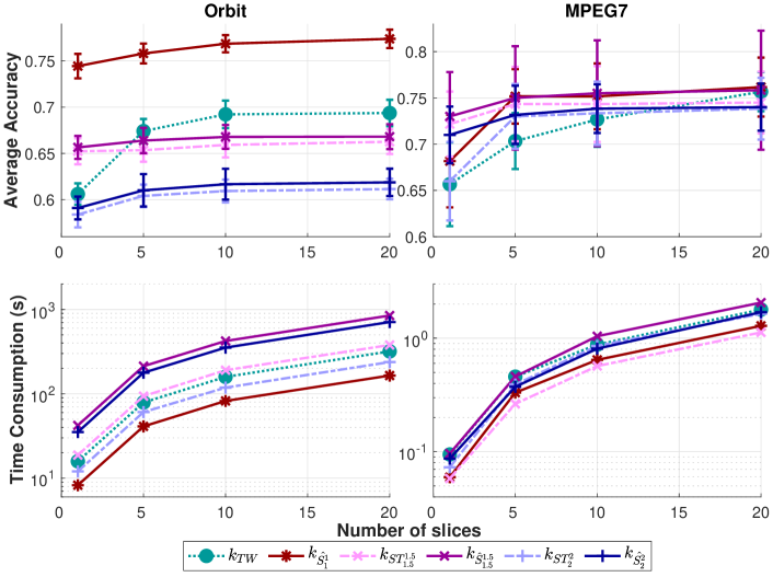
(b) With $M=100$.

Figure 22: SVM results and time consumption for kernel matrices of slice variants with graph ${\mathbb{G}}_{\text{Log}}$.

C.3 Further Discussions

For completeness, we recall important discussions on the underlying graph for Sobolev transport in Le et al. (2022), since they are also applied or adapted for the (regularized) Sobolev IPM in our work.

Measures on a graph.

In this work, we consider the (regularized) Sobolev IPM between two input probability measures supported on the same graph, which has the same setting as the Sobolev transport (Le et al., 2022).

The proposed kernels upon regularized Sobolev IPM are for input probability measures, i.e., to compute similarity between two probability measures, on the same graph. We distinguish our line of research to the following related problems:

$\bullet$ Compute distance between two (different) input graphs. For examples, Petric Maretic et al. (2019); Dong & Sawin (2020); Tam & Dunson (2022) compute OT problem (i.e., a specific instance of IPM) between two (different) input graphs, where their goals are to compute distance between two input graphs. They are essentially different to our considered problem which computes distance (i.e., regularized Sobolev IPM) between two input probability measures supported on the same graph.

$\bullet$ Graph kernels between two (different) input graphs. Graph kernels are kernel functions between two input graphs to assess their similarity. A comprehensive review on graph kernels can be found in Borgwardt et al. (2020); Kriege et al. (2020); Nikolentzos et al. (2021). Essentially, this line of research is different to our proposed kernels, i.e., regularized Sobolev IPM kernels to measures similarity between two input probability measures on the same graph.

Path length for points in graph ${\mathbb{G}}$ (Le et al., 2022).

We can canonically measure a path length connecting any two points $x,y\in{\mathbb{G}}$ where these two points $x,y$ are not necessary to be nodes in $V$ of graph ${\mathbb{G}}$.

Consider the edge $e=\langle u,v\rangle$ connecting two nodes $u,v\in V$, for $x,y\in\mathbb{R}^{n}$ and $x,y\in e$, we have

$$x=(1-s)u+sv,$$

$$y=(1-t)u+tv,$$

for some scalars $t,s\in[0,1]$. Thus, the length of the path connecting $x,y$ along the edge $e$ (i.e., the line segment $\langle x,y\rangle$) is equal to $|t-s|w_{e}$. Consequently, the length for an arbitrary path in ${\mathbb{G}}$ can be similarly defined by breaking down into pieces over edges and summing over their corresponding lengths (Le et al., 2022).

Extension to measures supported on ${\mathbb{G}}$.

Much as Sobolev transport (Le et al., 2022), the discrete case of the regularzed Sobolev IPM in Equation (10) can be easily extended for measures with finite supports on ${\mathbb{G}}$ (i.e., supports of the input measures may not be nodes in $V$, but possibly points on edges in $E$) by using the same strategy to measure a path length for support data points in graph ${\mathbb{G}}$. More precisely, we break down edges containing supports into pieces and sum over their corresponding values instead of the sum over edges.

About the assumption of uniqueness property of the shortest paths on ${\mathbb{G}}$.

As discussed in Le et al. (2022) for Sobolev transport, note that $w_{e}\in\mathbb{R}_{+}$ for any edge $e\in E$ in graph ${\mathbb{G}}$., it is almost surely that every node in $V$ can be regarded as unique-path root node since with a high probability, lengths of paths connecting any two nodes in graph ${\mathbb{G}}$ are different.

Additionally, for some special graph, e.g., a grid of nodes, there is no unique-path root node for such graph. However, by perturbing each node, and/or perturbing lengths of edges if ${\mathbb{G}}$ is a non-physical graph, with a small deviation, we can obtain a graph satisfying the unique-path root node assumption.

Besides that, for input probability measures with full supports in graph ${\mathbb{G}}$, or at least full supports in any cycle in graph ${\mathbb{G}}$, then it exists a special support data point where there are multiple shortest paths from the root node to it. In this case, we simply choose one fixed shortest path among them for this support data point (or we can add a virtual edge from the root node to this support data point where the edge length is deducted by a small deviation). In many practical applications (e.g., document classification and TDA in our experiments), one can neglect this special case since input probability measures have a finite number of supports.

About the regularized Sobolev IPM.

Much as Sobolev transport (Le et al., 2022), we assume that the graph metric space (i.e., the graph structure) is given. We leave the question to learn an optimal graph metric structure adaptively from data for future work.

About the graphs ${\mathbb{G}}_{\text{Log}}$ and ${\mathbb{G}}_{\text{Sqrt}}$ (Le et al., 2022).

For a fast computation, we use the farthest-point clustering method to partition supports of measures into at most $M$ clusters. Then, let the set of vertices $V$ be the set of centroids of these clusters, i.e., graph vertices. For edges, in graph ${\mathbb{G}}_{\text{Log}}$, we randomly choose $(M\log{M})$ edges; and $M^{3/2}$ edges for graph ${\mathbb{G}}_{\text{Sqrt}}$. We further denote the set of those randomly sampled edges as $\tilde{E}$.

For each edge $e$, its corresponding edge length (i.e., edge weight) $w_{e}$ is computed by the Euclidean distance between the two corresponding nodes of edge $e$. Let $n_{c}$ be the number of connected components in the graph $\tilde{{\mathbb{G}}}(V,\tilde{E})$. Then, we randomly add $(n_{c}-1)$ more edges between these $n_{c}$ connected components to construct a connected graph ${\mathbb{G}}$ from $\tilde{{\mathbb{G}}}$. Let $E_{c}$ be the set of these $(n_{c}-1)$ added edges and denote set $E=\tilde{E}\cup E_{c}$, then ${\mathbb{G}}(V,E)$ is the constructed graph.

Datasets and Computational Devices.

For the datasets in our experiments (i.e., TWITTER, RECIPE, CLASSIC, AMAZON for document datasets, and Orbit, MPEG7 for TDA), one can contact the authors of Sobolev transport (Le et al., 2022) to access to them. For computational devices, we run all of our experiments on commodity hardware.

Hyperparamter validation.

For validation, we further randomly split the training set into $70\%/30\%$ for validation-training and validation with $10$ repeats to choose hyper-parameters in our experiments.

The number of pairs in training and test for kernel SVM.

Let $N_{tr},N_{te}$ be the number of measures used for training and test respectively. For the kernel SVM training, the number of pairs which we compute the distances is $(N_{tr}-1)\times\frac{N_{tr}}{2}$. For the test phase, the number of pairs which we compute the distances is $N_{tr}\times N_{te}$. Therefore, for each run, the number of pairs which we compute the distances for both training and test is totally $N_{tr}\times(\frac{N_{tr}-1}{2}+N_{te})$. For examples, in Table 1, we list these number of pairs for kernel SVM for all datasets used in our experiments.

References

- Achlioptas et al. (2018) Achlioptas, P., Diamanti, O., Mitliagkas, I., and Guibas, L. Learning representations and generative models for 3D point clouds. In International conference on machine learning, pp. 40–49. PMLR, 2018.
- Adams et al. (2017) Adams, H., Emerson, T., Kirby, M., Neville, R., Peterson, C., Shipman, P., Chepushtanova, S., Hanson, E., Motta, F., and Ziegelmeier, L. Persistence images: A stable vector representation of persistent homology. Journal of Machine Learning Research, 18(1):218–252, 2017.
- Adams & Fournier (2003) Adams, R. A. and Fournier, J. J. Sobolev spaces. Elsevier, 2003.
- Andersen et al. (1988) Andersen, N. T., Giné, E., Ossiander, M., and Zinn, J. The central limit theorem and the law of iterated logarithm for empirical processes under local conditions. Probability theory and related fields, 77(2):271–305, 1988.
- Belkin et al. (2006) Belkin, M., Niyogi, P., and Sindhwani, V. Manifold regularization: A geometric framework for learning from labeled and unlabeled examples. Journal of machine learning research, 7(11), 2006.
- Berg et al. (1984) Berg, C., Christensen, J. P. R., and Ressel, P. (eds.). Harmonic analysis on semigroups. Springer-Verglag, New York, 1984.
- Birgé & Massart (1993) Birgé, L. and Massart, P. Rates of convergence for minimum contrast estimators. Probability Theory and Related Fields, 97:113–150, 1993.
- Blei et al. (2003) Blei, D. M., Ng, A. Y., and Jordan, M. I. Latent dirichlet allocation. Journal of machine Learning research, 3(Jan):993–1022, 2003.
- Borgwardt et al. (2020) Borgwardt, K., Ghisu, E., Llinares-López, F., O’Bray, L., Rieck, B., et al. Graph kernels: State-of-the-art and future challenges. Foundations and Trends® in Machine Learning, 13(5-6):531–712, 2020.
- Cuturi (2013) Cuturi, M. Sinkhorn distances: Lightspeed computation of optimal transport. In Advances in Neural Information Processing Systems, pp. 2292–2300, 2013.
- Divol & Lacombe (2021) Divol, V. and Lacombe, T. Estimation and quantization of expected persistence diagrams. In International conference on machine learning, pp. 2760–2770. PMLR, 2021.
- Dong & Sawin (2020) Dong, Y. and Sawin, W. COPT: Coordinated optimal transport on graphs. Advances in Neural Information Processing Systems, 33:19327–19338, 2020.
- Dudley (1978) Dudley, R. M. Central limit theorems for empirical measures. The Annals of Probability, pp. 899–929, 1978.
- Edelsbrunner & Harer (2008) Edelsbrunner, H. and Harer, J. Persistent homology-a survey. Contemporary mathematics, 453:257–282, 2008.
- Geer (2000) Geer, S. A. Empirical Processes in M-estimation, volume 6. Cambridge university press, 2000.
- Gretton et al. (2012) Gretton, A., Borgwardt, K. M., Rasch, M. J., Schölkopf, B., and Smola, A. A kernel two-sample test. The Journal of Machine Learning Research, 13(1):723–773, 2012.
- Hua et al. (2018) Hua, B.-S., Tran, M.-K., and Yeung, S.-K. Pointwise convolutional neural networks. In Proceedings of the IEEE conference on computer vision and pattern recognition, pp. 984–993, 2018.
- Husain (2020) Husain, H. Distributional robustness with IPMs and links to regularization and GANs. Advances in Neural Information Processing Systems, 33:11816–11827, 2020.
- Kolouri et al. (2020) Kolouri, S., Ketz, N. A., Soltoggio, A., and Pilly, P. K. Sliced Cramer synaptic consolidation for preserving deeply learned representations. In International Conference on Learning Representations, 2020.
- Kozdoba et al. (2024) Kozdoba, M., Perets, B., and Mannor, S. Sobolev space regularised pre density models. In Forty-first International Conference on Machine Learning, 2024.
- Kriege et al. (2020) Kriege, N. M., Johansson, F. D., and Morris, C. A survey on graph kernels. Applied Network Science, 5:1–42, 2020.
- Kusano et al. (2017) Kusano, G., Fukumizu, K., and Hiraoka, Y. Kernel method for persistence diagrams via kernel embedding and weight factor. The Journal of Machine Learning Research, 18(1):6947–6987, 2017.
- Kusner et al. (2015) Kusner, M., Sun, Y., Kolkin, N., and Weinberger, K. From word embeddings to document distances. In International conference on machine learning, pp. 957–966, 2015.
- Latecki et al. (2000) Latecki, L. J., Lakamper, R., and Eckhardt, T. Shape descriptors for non-rigid shapes with a single closed contour. In Proceedings of the IEEE Conference on Computer Vision and Pattern Recognition (CVPR), volume 1, pp. 424–429, 2000.
- Le et al. (2022) Le, T., Nguyen, T., Phung, D., and Nguyen, V. A. Sobolev transport: A scalable metric for probability measures with graph metrics. In International Conference on Artificial Intelligence and Statistics, pp. 9844–9868. PMLR, 2022.
- Le et al. (2023) Le, T., Nguyen, T., and Fukumizu, K. Scalable unbalanced Sobolev transport for measures on a graph. In International Conference on Artificial Intelligence and Statistics, pp. 8521–8560. PMLR, 2023.
- Le et al. (2024) Le, T., Nguyen, T., and Fukumizu, K. Generalized Sobolev transport for probability measures on a graph. In Forty-first International Conference on Machine Learning, 2024.
- Liang (2017) Liang, T. How well can generative adversarial networks learn densities: A nonparametric view. arXiv preprint, 2017.
- Liang (2019) Liang, T. Estimating certain integral probability metric (IPM) is as hard as estimating under the IPM. arXiv preprint, 2019.
- Liang (2021) Liang, T. How well generative adversarial networks learn distributions. Journal of Machine Learning Research, 22(228):1–41, 2021.
- Mikolov et al. (2013) Mikolov, T., Sutskever, I., Chen, K., Corrado, G. S., and Dean, J. Distributed representations of words and phrases and their compositionality. In Advances in neural information processing systems, pp. 3111–3119, 2013.
- Mroueh (2018) Mroueh, Y. Regularized finite dimensional kernel Sobolev discrepancy. arXiv preprint, 2018.
- Mroueh & Rigotti (2020) Mroueh, Y. and Rigotti, M. Unbalanced Sobolev descent. Advances in Neural Information Processing Systems, 33:17034–17043, 2020.
- Mroueh & Sercu (2017) Mroueh, Y. and Sercu, T. Fisher GAN. Advances in neural information processing systems, 30, 2017.
- Mroueh et al. (2018) Mroueh, Y., Li, C.-L., Sercu, T., Raj, A., , and Cheng, Y. Sobolev GAN. In International Conference on Learning Representations, pp. 5767–5777, 2018.
- Mroueh et al. (2019a) Mroueh, Y., Sercu, T., and Raj, A. Sobolev descent. In The 22nd International Conference on Artificial Intelligence and Statistics, pp. 2976–2985. PMLR, 2019a.
- Mroueh et al. (2019b) Mroueh, Y., Sercu, T., Rigotti, M., Padhi, I., and Nogueira dos Santos, C. Sobolev independence criterion. Advances in Neural Information Processing Systems, 32, 2019b.
- Müller (1997) Müller, A. Integral probability metrics and their generating classes of functions. Advances in Applied Probability, 29(2):429–443, 1997.
- Nadjahi et al. (2020) Nadjahi, K., Durmus, A., Chizat, L., Kolouri, S., Shahrampour, S., and Simsekli, U. Statistical and topological properties of sliced probability divergences. Advances in Neural Information Processing Systems, 33:20802–20812, 2020.
- Nickl & Pötscher (2007) Nickl, R. and Pötscher, B. M. Bracketing metric entropy rates and empirical central limit theorems for function classes of Besov-and Sobolev-type. Journal of Theoretical Probability, 20:177–199, 2007.
- Nietert et al. (2021) Nietert, S., Goldfeld, Z., and Kato, K. Smooth -Wasserstein distance: structure, empirical approximation, and statistical applications. In International Conference on Machine Learning, pp. 8172–8183. PMLR, 2021.
- Nikolentzos et al. (2021) Nikolentzos, G., Siglidis, G., and Vazirgiannis, M. Graph kernels: A survey. Journal of Artificial Intelligence Research, 72:943–1027, 2021.
- Ossiander (1987) Ossiander, M. A central limit theorem under metric entropy with L2 bracketing. The Annals of Probability, pp. 897–919, 1987.
- Petric Maretic et al. (2019) Petric Maretic, H., El Gheche, M., Chierchia, G., and Frossard, P. GOT: An optimal transport framework for graph comparison. Advances in Neural Information Processing Systems, 32, 2019.
- Peyré & Cuturi (2019) Peyré, G. and Cuturi, M. Computational optimal transport. Foundations and Trends® in Machine Learning, 11(5-6):355–607, 2019.
- Rieck et al. (2019) Rieck, B., Bock, C., and Borgwardt, K. A persistent Weisfeiler-Lehman procedure for graph classification. In International Conference on Machine Learning, pp. 5448–5458. PMLR, 2019.
- Singh et al. (2018) Singh, S., Uppal, A., Li, B., Li, C.-L., Zaheer, M., and Póczos, B. Nonparametric density estimation under adversarial losses. Advances in Neural Information Processing Systems, 31, 2018.
- Sparck Jones (1972) Sparck Jones, K. A statistical interpretation of term specificity and its application in retrieval. Journal of documentation, 28(1):11–21, 1972.
- Sriperumbudur et al. (2009) Sriperumbudur, B. K., Fukumizu, K., Gretton, A., Schölkopf, B., and Lanckriet, G. R. On integral probability metrics, -divergences and binary classification. arXiv preprint, 2009.
- Tam & Dunson (2022) Tam, E. and Dunson, D. Multiscale graph comparison via the embedded laplacian discrepancy. arXiv:2201.12064, 2022.
- Uppal et al. (2019) Uppal, A., Singh, S., and Póczos, B. Nonparametric density estimation & convergence rates for GANs under Besov IPM losses. Advances in neural information processing systems, 32, 2019.
- Uppal et al. (2020) Uppal, A., Singh, S., and Póczos, B. Robust density estimation under Besov IPM losses. Advances in Neural Information Processing Systems, 33:5345–5355, 2020.
- Wang et al. (2019) Wang, Y., Sun, Y., Liu, Z., Sarma, S. E., Bronstein, M. M., and Solomon, J. M. Dynamic graph CNN for learning on point clouds. ACM Transactions on Graphics (TOG), 38(5):1–12, 2019.
- Wu et al. (2019) Wu, W., Qi, Z., and Fuxin, L. Pointconv: Deep convolutional networks on 3D point clouds. In Proceedings of the IEEE/CVF Conference on computer vision and pattern recognition, pp. 9621–9630, 2019.
- Xu et al. (2020) Xu, M., Zhou, Z., Lu, G., Tang, J., Zhang, W., and Yu, Y. Towards generalized implementation of Wasserstein distance in GANs. arXiv preprint, 2020.
- Yurochkin et al. (2019) Yurochkin, M., Claici, S., Chien, E., Mirzazadeh, F., and Solomon, J. M. Hierarchical optimal transport for document representation. Advances in neural information processing systems, 32, 2019.
- Zhao & Wang (2019) Zhao, Q. and Wang, Y. Learning metrics for persistence-based summaries and applications for graph classification. Advances in neural information processing systems, 32, 2019.
Supplement to “Scalable Sobolev IPM for Probability Measures on a Graph”
The supplementary is organized into three parts as follows:
Notations.
Let be the indicator function, i.e.,
For two points , let be the line segment in connecting the two points , and denote for the same line segment but without its two end-points.