Project 8 Collaboration
Dynamics of Magnetic Evaporative Beamline Cooling for Preparation of Cold Atomic Beams
Abstract
The most sensitive direct neutrino mass searches today are based on measurement of the endpoint of the beta spectrum of tritium to infer limits on the mass of the unobserved recoiling neutrino. To avoid the smearing associated with the distribution of molecular final states in the T-He molecule, the next generation of these experiments will need to employ atomic (T) rather than molecular (T2) tritium sources. Following production, atomic T can be trapped in gravitational and / or magnetic bottles for beta spectrum experiments, if and only if it can first be cooled to millikelvin temperatures. Accomplishing this cooling presents substantial technological challenges. The Project 8 collaboration is developing a technique based on magnetic evaporative cooling along a beamline (MECB) for the purpose of cooling T to feed a magneto-gravitational trap that also serves as a cyclotron radiation emission spectroscope. Initial tests of the approach are planned in a pathfinder apparatus using atomic Li. This paper presents a method for analyzing the dynamics of the MECB technique, and applies these calculations to the design of systems for cooling and slowing of atomic Li and T. A scheme is outlined that could provide a current of T at the millikelvin temperatures required for the Project 8 neutrino mass search.
I Introduction
The unknown absolute value of the mass of the neutrino is one of the most glaring holes in our understanding of particle physics today. The most sensitive direct search for neutrino mass to date is the currently running KATRIN experiment, which reconstructs the energies of electrons emitted in beta decays of molecular tritium (T2) using a MAC-E filter [1]. This technique establishes the endpoint shape of the beta spectrum, leading to the current world-leading direct upper limit of at 90% confidence level (CL) [2]. Cosmology is sensitive to the sum of the neutrino masses, although with assumptions about the physics of the early Universe, delivering upper limits below the KATRIN bound [3]. Neutrinoless double beta decay is also a probe of neutrino mass, if and only if the neutrino is a Majorana particle [4], although given uncertainties about the neutrino nature, mass orderings, and mixing parameters, without an observation no upper limit can be drawn. Finally, neutrino oscillations have proven definitively that at least two of the neutrino mass eigenstates have non-zero masses [5], setting lower limits on the electron-flavor-weighted neutrino mass in beta decay searches at 9 meV (normal mass ordering) and 48 meV (inverted mass ordering) respectively [6]. These values serve as targets for future generation neutrino mass searches, substantially below the present limits from both KATRIN and cosmological data. Since KATRIN has effectively saturated the power of both the MAC-E filtering technique and of T2, paradigm-shifting new technologies are required to enable further progress.
One promising method to advance the precision of neutrino mass measurements in the laboratory is cyclotron radiation emission spectroscopy (CRES) of electrons produced in decays of T [7, 8, 9, 10]. In this technique, electron energy is accessed with great precision by measuring cyclotron frequencies in a magnetic trapping field. To achieve sensitivities significantly below the KATRIN goal of at 90% CL (the Project 8 target is 40 meV at 90% CL), CRES must be complemented by an atomic T source, since T2 introduces irreducible systematic uncertainties associated with excitation of molecular final states [11]. Realization of a high throughput atomic source, delivering a sufficient atom current to enable a sensitive neutrino mass measurement through beta decay endpoint studies of magnetically trapped T, is one of the primary R&D goals of Project 8 in the next decade.
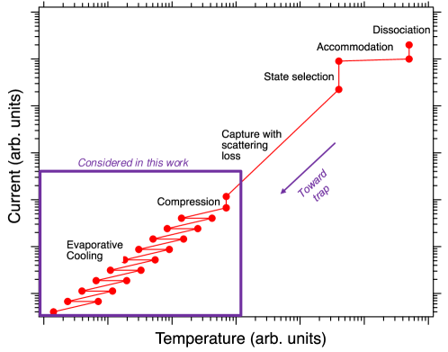
The proposed Project 8 trap is vertically oriented, and closed magnetically at its lower extreme to hold atoms gravitationally in the upward direction. Magnetogravitational traps have been used successfully for containment of ultra-cold neutrons [12, 13, 14, 15]. This configuration contains T while avoiding accumulation of large numbers of low-pitch-angle electrons that are invisible to the CRES system but cause problematic heating and charge accumulation, and can scatter to observable pitch angles, creating needless lower-energy background. The T cooling stage must operate continuously in the atomic beamline fed by a source of initially hot T atoms. Multiple source configurations are under investigation. Approaches based on thermal cracking produce an initial flux at 2200 K [16], whereas electron cyclotron resonance sources [17] may provide a somewhat more modest initial temperature source. In either case, an intermediate stage of cooling can be then be performed by scattering T off cold surfaces in a process known as accommodation to between 10 and 30 K, below which temperature the T2 vapor will freeze to solid surfaces and be taken out of circulation. In previous experiments with hydrogen, further cooling has been achieved by down-scattering the atomic vapor from a film of superfluid liquid helium [18]; however, in the case of tritium this technique is not expected to be effective, as the larger physisorption energy indicates that recombination will be unavoidable at the T-He interface [19]. Though we lack direct experimental confirmation that this approach will not work for T, the issue of potentially problematic physisorption prompts us to explore other methods of cooling and trapping as the Project 8 baseline. A crucial technical step is the further cooling of a large flux of moderately cold atomic T to millikelvin temperatures with high throughput, minimal recombination, high purity, and continuous operation.
The Project 8 collaboration is pursuing R&D on a Magnetic Evaporative Cooling Beamline (MECB) for this purpose. This scheme is based on the pioneering work of Hess [20, 21] that eventually led to successful Bose Einstein condensation of atomic H [22, 23]. For Project 8, evaporative cooling is implemented continuously as a function of the axial coordinate of a linear atom guide, rather than in a single position as a function of time, as employed in magneto-optical traps [24]. Devices exhibiting dynamics of this sort but using radio frequency excitation to perform the evaporation cut have been discussed for heavier atoms, see, for example, Refs [25, 26]. Application to atomic T carries unique additional challenges that will be elaborated below. Under the MECB scheme, low-field-seeking spin polarized atoms are confined radially within a cylindrical magnetic potential well. The highest energy atoms are selectively rejected as the cloud travels along the beamline. Assuming the population remains in thermal equilibrium, the fractional energy loss per unit time will exceed the fractional loss of particles, leading to cooling. The method proposed here uses only magnetic fields and no lasers; this distinction is important for the atomic T application, where laser cooling is ineffective because available continuous-wave lasers do not exist with sufficient power at the challenging 121 nm wavelength associated with the Lyman alpha line, the only accessible spectral feature from the T ground state.
One of the demonstrator phases en route to this system is a cold atomic lithium (Li) beamline, providing the opportunity to prove the technique and quantitatively study its dynamics with a more convenient atomic source. This technology development platform is advantageous, since Li is non-radioactive, experiences similar magnetic trapping forces to T, and is laser addressable via the D lines for density mapping and Doppler thermometry to monitor thermalization, cooling and slowing. A tunable flux of pre-cooled 6Li will be delivered from an oven via a Zeeman slower [27, 28, 29], enabling beam parameters to be tuned to replicate those expected to emerge from the T accommodator in the final Project 8 beamline. A key goal of this pathfinder experiment is to validate quantitative models of MECB dynamics. The tools we describe in this paper have been developed both to study the performance of a possible MECB implementation using atomic T for Project 8, and to provide design specifications for the atomic 6Li pathfinder project and predictions for its performance.
The approaches presented in this work are not the only conceivable schemes for slowing a fast-moving atomic beam of T. An ingenious method for slowing polar molecules in a spinning electrostatic guide has been developed by Chervenkov et al. [30] and a similar approach is possible for magnetic atoms. H and D have been Zeeman slowed in multi-stage decelerators [31] and atomic coil gun geometries [32]. However, for any of these approaches, operating them at the very high atom currents needed for the Project 8 application and in the difficult environment of a tritium handling facility remains to be demonstrated, and appears to be very technically challenging.
In what follows, we outline a new method of analysis of MECB dynamics (Sec. II), discussing trapping in the relevant magnetic multipole fields (Sec II.1), the dynamics of evaporative beam cooling (Sec II.1) including details of cross sections (Sec II.3) and collision calculations (Sec II.4), followed by an analysis of the proposed slowing method via transverse perturbation (Sec II.5). We then use these tools to predict the performance of a MECB geometry designed for 6Li cooling and slowing (Sec III). Finally, we will provide a speculative picture of a possible atomic T cooling MECB geometry for Project 8 (Sec IV) and present our conclusions (Sec V).
II Theory of the magnetic evaporative cooling beamline
The MECB scheme for Project 8 is in an advanced state of conceptual development. In this section we review the key concepts that are central to its operation, in particular, methods of laser-less trapping, cooling and slowing in linear magnetic multipole geometries.
II.1 Trapping in magnetic multipole guides
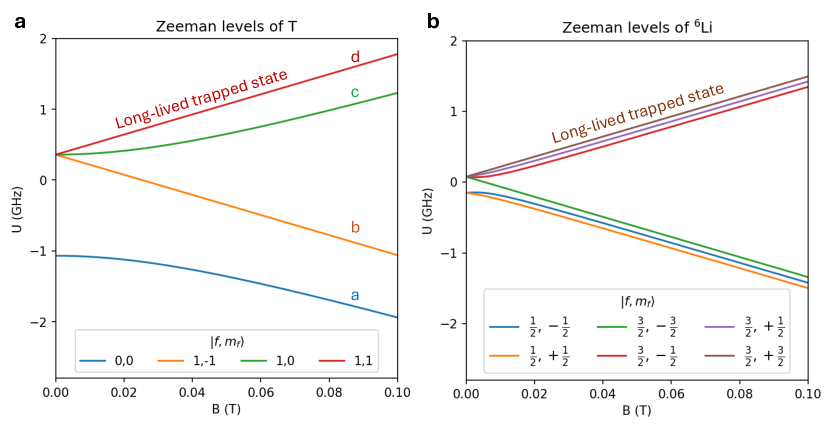
Investigations into spin polarized atomic H and 6Li have been widespread in AMO physics [33, 34, 35, 36, 37]. Trapping of these species relies on the interaction of the atom, which in each case has a single unpaired outer electron, with applied magnetic fields. In both of these atoms, the nucleus also has a non-zero spin (1/2 for T and H, and 1 for 6Li). In the case of H or T, the nuclear and electron spin can therefore couple in either a singlet (F=0) or a triplet (F=1) configuration. This coupling leads to two possible hyperfine levels at zero field. At non-zero magnetic field, these levels are further split by the Zeeman effect, since the interaction between the electron and nucleus with the external field generates inequivalent energy perturbations, in each case proportional to where is the mass of the electron (e) or nucleus (N), respectively. The four resulting Zeeman-split levels of hydrogen and tritium are commonly denoted in the literature as , from least to most energetic. In the case of 6Li, the nucleus has spin 1. There are still two hyperfine levels at zero field, this time corresponding to doublet (F=1/2) and quadruplet (F=3/2) total spin configurations, and applied B fields split this into a manifold of 6 Zeeman levels. The Zeeman-split energy levels can be calculated nonperturbatively using the Breit-Rabi method, diagonalizing the relevant Hamiltonian to account consistently for both Zeeman and hyperfine effects, with results shown in Fig 1. The eigenstates can be labeled as , the states to which they are adiabatically connected as .
At large magnetic field the Zeeman perturbation dominates over the hyperfine one, and because it is the coupling of the electron spin to the field that is dominant in determining the energy of a given level. The states thus split into two groups: the so-called “high-field seekers” where the electron spin is predominantly anti-aligned (and hence magnetic moment aligned) with the magnetic field whose energies fall as the field strength increases; and “low-field seekers” where the electron spin is predominantly aligned with the field whose energies increase with increasing field. Magnetic fields can admit static minima in free space but not static maxima, and as such only the low-field-seeking states can be trapped in a time-invariant magnetic potential. Because the unpaired electron dominates the trap strength, the depths of a given potential well for low-field seekers of T, 6Li, or indeed any other alkali metal are remarkably similar.
Although all low-field-seeking states can be trapped, not all can be expected to exhibit a long trap lifetime. In the case of T, the state (which adiabatically connects to ) is composed of electron and nuclear spin states as , with small mixing parameter . These states can be lost through spin-exchange collisions , , and [38]. After a significant time period therefore, only states are expected to remain in a magnetic trap. A similar argument suggests that in the case of 6Li, the state analytically continuing to is the one that can be expected to enjoy a long trap lifetime. These trapped states are labeled in Fig. 1.
The discussion so far has suggested magnetic fields varying in magnitude but always aligned or anti-aligned with the atomic spin. A moving atom, however, can move across magnetic fields pointing in different directions. In geometries where the B field direction is changing relatively slowly in space, the adiabatic theorem says that the spin state will rotate to follow the direction of the field [39]. As such, provided that the adiabatic condition is met, it is only the magnitude of a magnetic field, not its direction, that determines the trapping potential for low-field-seekers. As a consequence of this principle, effective atom traps can be made using linear magnetic multipoles. Other trapping geometries including Halbach arrays [40] and Ioffe traps [41] are also in common use as atom traps and could be considered as elements of a future atomic tritium source.
A multipole magnetic field configuration can be expressed analytically as real and imaginary parts of the following complex expression [42]
| (1) |
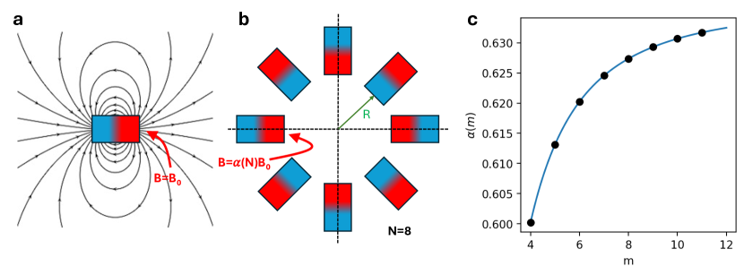
The magnetic field strength is at reference radius , which fixes the constant . A field that is predominantly of multipole order can be generated by arranging permanent magnets at a fixed radius and uniformly spaced angles, with an alternating North-inward / South-inward ordering, as shown in Fig. 2. The average magnetic field at the radius of the inner magnet surface in this configuration is not exactly equivalent to the surface field of an individual magnet in vacuum , due to the segmentation of the geometry. If magnetic dipole elements with inner and outer radius and respectively form the multipole then the resulting field can be shown to be given by [40]
| (2) |
For a thick magnet, and we find that
| (3) |
The function is an order-1 number that encodes the effects of segmentation of the magnet geometry, in Fig. 2, c.
Fig 3, a shows geometrical multipole field maps for a quadrupole and octupole guide. Fig. 3, b shows the radial dependence of the field strength, scaled to the surface field of the magnet, accounting for the finite segmentation correction . We now proceed to analyze the trapping and cooling in multipole guides analytically. A table of variable names can be found in Appendix B.
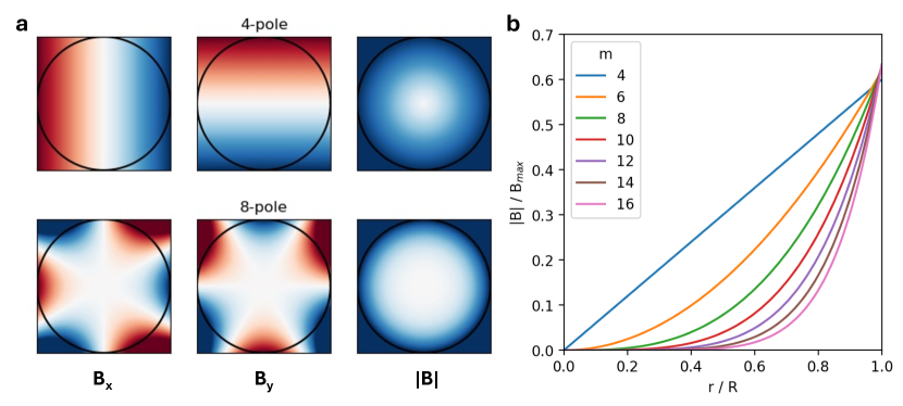
The trapping potential can be obtained by taking the magnitude of the field,
| (4) |
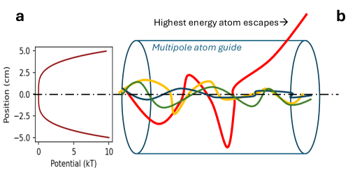
Low-field seeking atoms will tend to thermalize toward the center of the guide because this is where is the smallest. Furthermore, the larger the multipolarity, the flatter the trap and lower the field gradient shape near the center. For a fixed individual magnet element surface strength , a higher multipolarity will hold a given number of atoms at a lower average density. This principle will be relevant in the discussion of cooling geometry that follows. If atoms with mass are allowed to thermalize into a linear multipole guide and the trapping potential is large enough to effectively trap the atoms (i.e. ), they will become distributed in position and momentum according to the Boltzmann distribution,
| (5) |
where D is a normalization constant that fixes the total number of atoms. This expression allows for a mean transverse momentum along the multipole, since the atoms are not trapped in this direction, and the density at any position can be obtained by integrating the distribution function over the momentum degrees of freedom,
| (6) |
Eq. 5 has the notable property that the momentum and position dependencies are factorizable, which means that in an equilibrated beam the velocity and position distributions are decoupled, simplifying calculations. For a steady state beam that is moving along , we can express the normalization factor in terms of the beam particle throughput, by noting that if there is a bulk velocity then the current of atoms through a given surface is related to the particle density as
| (7) |
which gives in terms of and , with the result that
| (8) |
We have introduced above the barrier height parameter, which encodes the depth of the trapping field in units of ,
| (9) |
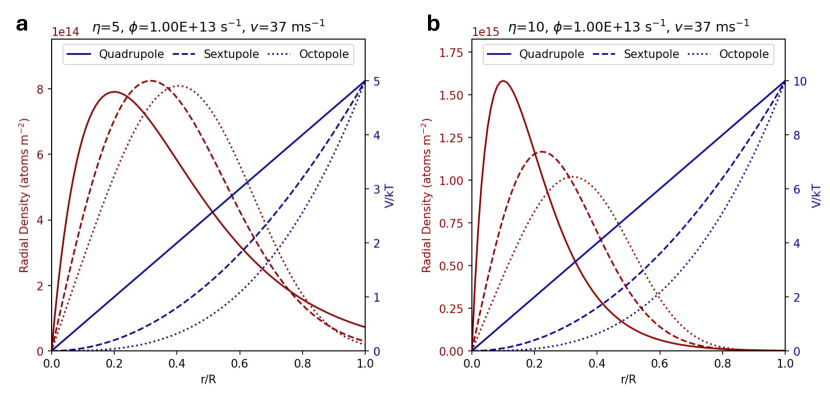
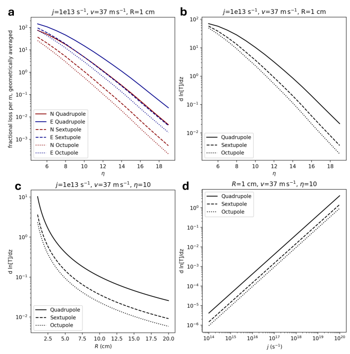
where is the smallest maximum value of the magnetic ‘wall’ field encountered by atoms. Fig. 4 shows fixed density plots at fixed R=1 cm showing the radial density of atoms in an equilibrated system compared against the radial potential curve for some representative cooling parameters and two values of evaporative barrier height .
II.2 Analytic treatment of evaporative cooling in a guide
Atoms will evaporate if their transverse kinetic energy exceeds the magnetic potential at the wall. The escape criterion can be defined in terms of the threshold energy scale parameter . As atoms evaporate, the remaining trapped atoms must, through collisions, regain a new equilibrium temperature.
A gas of atoms trapped in a 3D well has a total energy made up of the kinetic energy and the potential energy . The virial theorem relates the average kinetic and average potential energies of particles bound by a potential. If the potential is of the form , then:
| (10) |
where is the dimensionality of the well. For an -pole magnet the potential power dependence is . For example, in an infinite quadrupole 2D well the potential is linear in , and . The rate of evaporative cooling from a guided beam depends on the multipolarity of the guide via the potential power law , and the barrier height . In a seminal paper [20], Hess advanced an early analytic model to illustrate the dynamics of evaporative cooling. The Hess model is in fact incomplete, since it neglects the density of energy states in the trap, but it is informative of the basic principles of evaporative cooling, and becomes relatively accurate in the limit and hence . In this case, the rate of change of energy of the gas is determined by the evaporative cooling power
| (11) |
where the evaporative cooling power depends on the cut threshold via
| (12) |
Here is an order-one number characterizing the mean excess energy of an atom escaping over the potential barrier. Hess [20] suggests that this quantity is typically 2 per particle, but it can be can shown that for a flat trap with , , corresponding to the average energy of the Maxwell Boltzmann distribution over an energy cut .
We consider only evaporation in this analysis. Other loss terms arise from spin-flip and dipolar losses, and from scattering of atoms in the background gas, though our quantitative estimates suggest that these are significantly sub-leading. One is also free to interchange kinetic and potential energy components without loss by suitable variations of the magnetic confinement. Hess includes such a term when part of the cooling is achieved by isentropic expansion via reduction of the magnetic field. The value of can be kept constant by lowering the magnetic guide ‘wall’ height as the gas cools, such that (ideally) and track one another.
When the gas is not stationary as in Hess’s analysis but is collectively moving along a magnetic guide, the kinetic energy of the bulk motion brings in new terms to the above equations. This additional kinetic energy is not in equilibrium with the internal temperature of the gas because in a magnetic guide there is no viscosity or friction (unless special measures are taken to introduce it). If the mean bulk velocity is the kinetic energy per atom is , which we may write as to avoid carrying Boltzmann’s constant in the equations. Each atom that evaporates now takes this additional kinetic energy with it. The evaporative cooling power becomes
| (13) |
Not all of this power is available to cool the internal gas temperature. Similarly, the total energy now includes the bulk kinetic energy and the energy flow becomes:
| (14) |
As expected, the bulk kinetic energy plays no role in cooling in this case.
| (15) |
Setting , as expected for
| (16) |
The pure number is termed the cooling exponent. Integrating,
| (17) |
where is a constant of integration.
In Fig. 5 are shown two strategies from a continuum of possibilities for adjusting the field strength to keep constant as the gas cools.
In the left-hand plot the guide potential is not changed and atoms settle into ever lower potentials as they cool. It offers the advantage of shrinking the beam diameter steadily, desirable to keep the density up as the beam cools and loses particles. In the right-hand plot the field is reduced but the size of the magnetic guide is the same.
A key principle omitted from the analysis of Hess is that the energy distribution of atoms thermalized into a potential well will have a non-trivial density of states in total energy , deviating from a Maxwell Boltzmann distribution by a density-of-states factor . An analytic model of the evaporative cooling process that includes this effect and hence is applicable for finite was provided by Davis et al. in Ref [43]. Under this model, a trapping potential is applied that scales like along of the axes, with no trapping in of them ( is thus the dimensionality of the trap). In such a trap, the fraction of particles with energy below some cut is
| (18) |
where is a density of states function, which for an trapping potential is, following from Eq. 8,
| (19) |
with a constant. The chemical potential fixes the normalization of the distribution, and we can solve for it through applying the constraint,
| (20) |
Finding in this way and then re-expressing the energy in terms of dimensionless variable we find the following expression for the fraction of the particles that lie above ,
| (21) |
where with one or two arguments represents the complete or incomplete gamma function, respectively. The mean energy lost per particle leaving the trap (which we have called ) can be found by calculating the weighted energy of the particles with , which is given in terms of the ratio of two incomplete gamma functions by
| (22) |
To find the cooling exponent, we require the fraction of particles and energy below energy cut , and then we can obtain via
| (23) |
Evaluating these two integrals,
| (24) |
| (25) |
we obtain an expression for that accounts for the trap density of states for finite multipolarity ,
| (26) |
This is notably different from the value of provided in the original work of Hess [20], which is, in this notation,
| (27) |
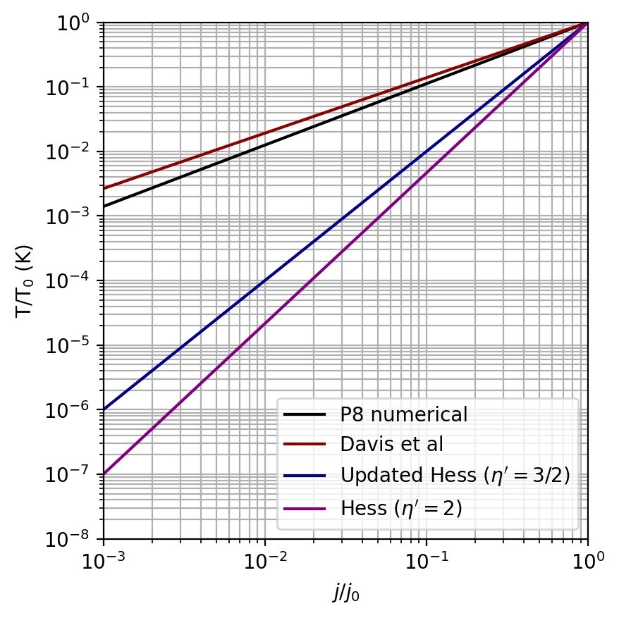
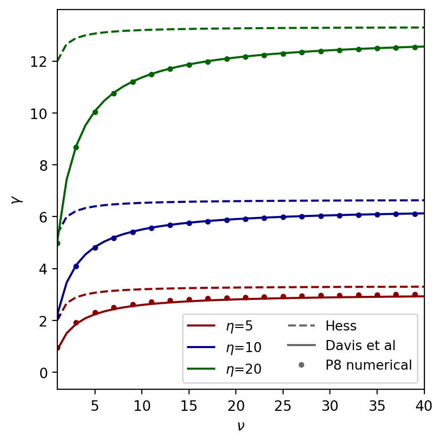
In the case of fixed guide geometry and evaporation cut , the achievable temperature reduction for a given atom transport efficiency scales as a power law with exponent , per Eq. 17. Fig. 6 compares the predictions given various predictions discussed above, for a finite quadrupole with to the numerical model advanced in this work. Fig. 7 compares the Hess and Davis models for various values of the multipolarity and also compares against the numerical model that will be presented in subsequent sections of this work. In all models, we observe the general trend that cooling efficiency for a specific temperature drop is better for larger multipolarity and for larger evaporation cut . Both figures show good agreement between the numerical solutions of this work and the Davis model which incorporates the density of states effect, and clarify the regimes where the Hess approximation may be taken to be a valid one. At the multipolarities of interest to this study the Hess approximation provides an imperfect prediction for the cooling exponent , but as the multipolarity becomes large the Hess approximation becomes increasingly accurate. This correspondence occurs because at large the trap becomes flatter, and the energy density of states factor well approximates the Maxwell Boltzmann expectation over most of the volume of the trap.
We turn now to the problem of slowing the longitudinal component of the bulk motion, under the simple flat-potential Hess model. We consider slowing the beam by transferring longitudinal energy to transverse for evaporative cooling. The transfer is effected by introducing magnetic perturbations along the beamline to mimic a viscous or “friction” force. The additional transverse energy is evaporated away, if the beam is dense enough to regain thermal equilibrium. The perturbations can be quasi-continuous (the beam is consistently slowed down during cooling) or discrete (the beam is slowed in steps between evaporative cooling segments).
We first consider the quasi-continuous case. The energy flow in the quasi-continuous-slowing example becomes
| (28) |
We introduce the “mass flow number”, which is the ratio of the bulk transport velocity to the mean thermal speed in the co-moving frame
| (29) |
which is also related to the “Mach number” via , with the adiabatic constant for an ideal monatomic gas (though notably, spin-polarized Li and T do not necessarily exhibit the thermophysical properties of a simple monatomic gas due to the long-range triplet potentials between atoms [44]). The longitudinal kinetic energy may be written conveniently in terms of the :
| (30) |
We assume that the mass flow number , in the quasi-continuous scenario, is constant as the beam is cooled. The evaporative cooling power is
| (31) |
Then,
| (32) | |||||
| (33) |
To avoid excessive beam losses , which in turn implies
| (34) |
Large mass flow numbers force the use of large values of but large values of make the process very slow because atoms carrying that much energy are rare. The smallest value of in directed flow is for effusive flow from an orifice, for which the mean longitudinal velocity is
| (35) |
and hence
| (36) |
This value increases by about 1. Larger values are better for assuring atoms generally flow forward in the beam.
The discrete-perturbation approach to slowing the beam turns out to be more efficient (less costly in evaporated atoms). In this approach atoms keep the same longitudinal speed while undergoing transverse cooling, and then encounter a step perturbation that reheats the beam and slows the bulk motion. The process is repeated until the desired temperature is reached. The advantage over continuous cooling is that the evaporation to cool the bulk motion is carried out with hotter atoms that carry away more energy per atom. The magnetic wall height must be increased as necessary at each step to maintain efficiency.
The transverse cooling takes place as before, but since , the term is absent in the cooling exponent. The amount of reheating depends on the initial kinetic energy entering a section and the amount that remains on entering the next section. The cooling sections change and but not , whereas the slowing sections change and but not . The beam parameters at three points along the axis of each section are hence as follows: gives the particle number, bulk kinetic energy per particle, and temperature on entering a transverse-cooling section; gives those parameters at the end of the section and before the perturbation; and gives the parameters after the perturbation and at the entrance to the next cooling section. In the cooling section the bulk kinetic energy does not change and is as given in Eq. 16. The particle loss in this section is
| (37) |
We assume the perturbation can be tuned so that the mass flow number entering each cooling section is always the same. Then
| (38) | |||||
| (39) |
The reheating of the beam is
| (40) | |||||
| (41) | |||||
| (42) |
Applying this equation and Eq. 37 repeatedly in a cascade of cooling steps, one can arrive at a final temperature and particle number, and some examples of such cooling trajectories are later calculated and present in Figs. 18,20. While several parameters present themselves for optimization, in practice one cannot depart far from and for reasonable speed in cooling without excessive particle loss.
The models discussed in this section provide some indications of the relevant scaling laws for performance parameters in a MECB system. Even in the most advanced models, however, no information about times and distances can be obtained without appending a detailed treatment that involves cross sections, beam dimensions, currents, and other inputs. The rate of evaporation depends on competition between thermalization and particle and energy losses. We will first evaluate numerically the cooling power in practicable geometries, and then return to consider a more detailed analytic model for comparison.
II.3 Triplet scattering cross sections
| Species | Triplet s-wave | Cross Section |
|---|---|---|
| H | 70 pm | |
| T | -4200 pm | |
| 6Li | -11900 pm | |
| 7Li | -144 pm |
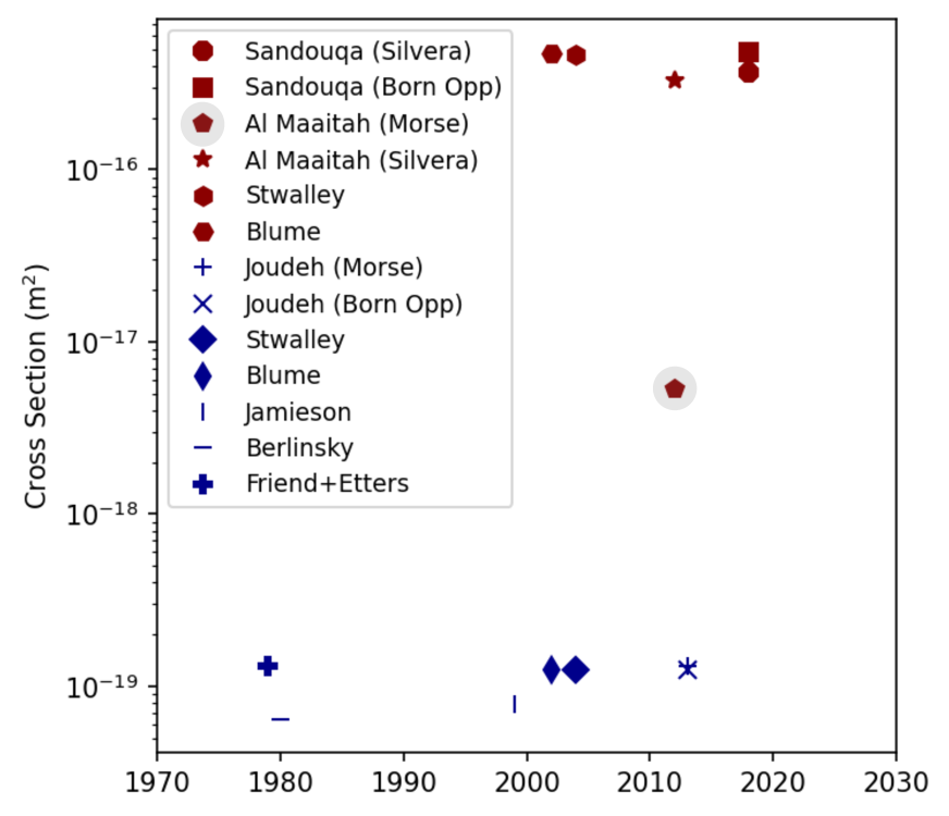
For a thermalized distribution in a potential well, individual atoms are constantly interacting with one another, randomly sharing their energy to maintain a Maxwell Boltzmann distribution. The frequency of collisions that eject atoms from the guide and lead to cooling, as well as the frequency of collisions that redistribute energy to re-thermalize the distribution, is dictated by the local density of atoms at each position in the guide as well as the triplet scattering cross section . Because T atoms are indistinguishable bosons, any combination of low-field-seeking hyperfine states will undergo s-wave triplet elastic scattering. For low energy collisions of identical particles, can be expressed exclusively in terms of the triplet s-wave scattering length via . The scattering length can, in turn, be calculated from interatomic potentials. A popular potential for atomic H and T calculations is the Silvera potential [45], which is derived from a multi-parameter fit to numerical solutions of the Schrödinger equation for pairs of atoms at fixed separation that was evaluated in Ref [46]. The Morse [47] and Born Oppenheimer [48, 49] potentials provide alternatives.
Solution of the Schrödinger equation in the presence of these potentials provides the s-wave phase shift, and hence the scattering length. The challenge of these calculations lies in the fact that the scattering length is very sensitive to the repulsive core of the potential, and small changes to this shape can have a dramatic impact on the final result. Calculations of the s-wave triplet cross section for H-H scattering have been performed by Joudeh [50], Stwalley [51], Blume et al. [49], Jamieson et al. [48], Berlinsky[52], and Friend and Etters [22], with a consensus value of Å in the low temperature limit, where the relative momentum in the collisions tends toward zero. T-T cross section calculations have been presented by Sandouqa and Joudeh [44], Al Maaitah [53], Stwalley [51], and Blume [49] and suggest much larger value of 37 Å, corresponding to a scattering cross section nearly four orders of magnitude larger for T-T than for H-H. For the purposes of evaporative cooling, this increased scattering length is highly beneficial as it results in much faster thermalization of the interacting atomic vapor, and relaxes the beam density requirement. Fig 8 shows the calculated s-wave cross sections collected from the aforementioned literature, for H-H and T-T scattering. Apart from one outlier highlighted in grey (T-T scattering using the Morse potential), the literature provides a consistent picture of the expected triplet scattering lengths relevant for evaporative cooling.
For 6Li, the triplet scattering cross sections have been calculated in Ref [54] (-) and Ref [55] (-2240 ) based on potentials from Refs [56, 57, 58, 59, 60, 54].
For present purposes we take values for the relevant cross sections to be those tabulated in Fig. 8, right, which are representative of the available theoretical literature, with 6Li having s-wave triplet cross section of m2 and T having . The additional complication associated with the vanishing triplet scattering cross section for identical fermions in the case of 6Li is not prohibitive in this geometry, as the travel time in the beam is insufficient for significant relaxation of the non-stretched states to occur. The Li beam will instead be comprised of a mixture of the low-field-seeking hyperfine states, thus maintaining the large triplet scattering cross section even at very low temperature. The increased cross section of Li over T implies that the Li demonstration apparatus can operate at somewhat lower current and hence lower instantaneous beam density than the T apparatus, making it possible to explore these techniques with currently available oven-based sources and Zeeman slowing systems.
II.4 Beam cooling via evaporation
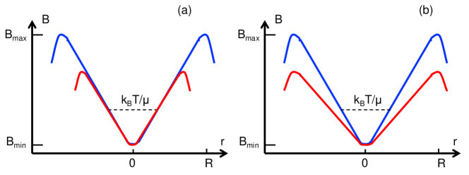
Evaporation occurs as a result of particles randomly receiving an upward fluctuation in energy following a collision, that leads them to have enough transverse momentum to escape from the guide. Both the shape of the potential and a cartoon illustrating the evaporation dynamics are shown schematically in Fig. 9, a.
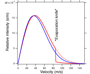
Any trapped gas will eventually attain a local Maxwell Boltzmann distribution through thermalizing collisions, and an evaporation cut can be applied to the high tail of this distribution. The highest energy subset of particles will then escape, leaving only a small tail of still-escaping atoms above the energy cut (indicated by the red curve in Fig. 9, b). The remaining particles redistribute energy through further collisions, leading to a lower temperature Maxwell Boltzmann distribution (the blue curve in Fig. 9, b). These collisions also redistribute energy between the and directions, which implies that the temperature in the longitudinal and transverse directions (quantified via the spread of the momentum phase space distribution) is always isotropic. The collisions conserve both total energy and total momentum, so while the distribution is cooled to a smaller phase space volume, its mean momentum remains constant (assuming there is no preferential evaporation direction, valid in the the case of a radial evaporation cut). A thermalized beam in a linear multipole guide will thus maintain a mean momentum in the direction, while it cools. This implies that the challenge of producing a beam to load a stationary trap has two components: cooling, which involves reducing the width of the thermalized momentum phase-space distribution; and slowing, which involves removing the mean momentum. Both of these goals can be accomplished in static magnetic geometries, and in this section and the next we outline the methods to calculate their effectiveness in representative geometries.
The equipartition theorem states that for a well-thermalized distribution, the linear energy density in a given -slice of the guide of width will be
| (43) |
Here is the number of particles between and . The kinetic and potential energy distributions can be evaluated for a thermalized distribution, as
| (44) |
Fig. 10 shows examples of the kinetic and potential energy distributions across the beam for some representative multipole configurations. We are interested in the rates of change of particle number and energy with , which we denote as . For a beam moving with bulk velocity these can be connected to the time derivatives in the beam co-moving rest frame, via
| (45) |
As a result of Eq 43, the change in temperature as a function of longitudinal position along the beam can be found in terms of the losses in energy and particle number due to evaporation, as
| (46) |
To obtain and we must obtain the evaporation rates, integrated over the spatial density distribution in the guide. A particle will leave if its transverse momentum following a collision is more than the trap depth, when accounting also for potential energy at the location of the collision. The critical momentum for loss of particles at each position is thus given by
| (47) |
The rate of particles obtaining momenta above this value from collisions is obtained from the time dependence of the phase space distribution at each position. In a generic out-of-thermal-equilibrium system this time dependence can be obtained from the Boltzmann transport equation,
| (48) |
whose terms represent, from left to right: time evolution of phase space, mass flow due to inertia, force from applied potential, and collision integral that leads to thermalization. For spherical collisions, has the form
| (49) |
The momentum delta functions enforce energy conservation in two-body collisions where indices 1,2 label the initial state and 3,4 the final state. To quantify evaporation rates, the relevant contribution to the phase space distribution is that associated with the collision integral . The relevant loss rates of position-dependent kinetic energy density, potential energy density and particle density can be obtained by numerical integration of the out-of-equilibrium phase space distribution with an appropriate transverse momentum cut applied, as
| (50) |
| (51) |
The time derivatives appearing in the above equations encode the change in the phase space distribution function due to redistribution of the ensemble energy and momentum during evapor ation. This time derivative can be evaluated via the full collisional Boltzmann transport equation, as presented in Appendix A.
Our numerical simulations show that these calculated loss rates obey very closely the expected scaling relations with temperature, cross section and density, allowing them to be evaluated once for each value of in conditions and and applied at generic and via, for example,
| (52) |
These quantities evaluated in reference conditions and used in the calculations that follow are shown in Fig. 11. To obtain the total energy and particle number loss rates and hence the longitudinal temperature evolution via Eq. 46, the kinetic, potential and particle losses must be integrated over the transverse geometry of the guide, applying the appropriate momentum cut at each position. These integrals take the form
| (53) |
| (54) |
Since the whole distribution is co-moving along the guide at velocity , the z dependent loss rates can be found from these time dependent rates with a factor of the velocity,
| (55) |
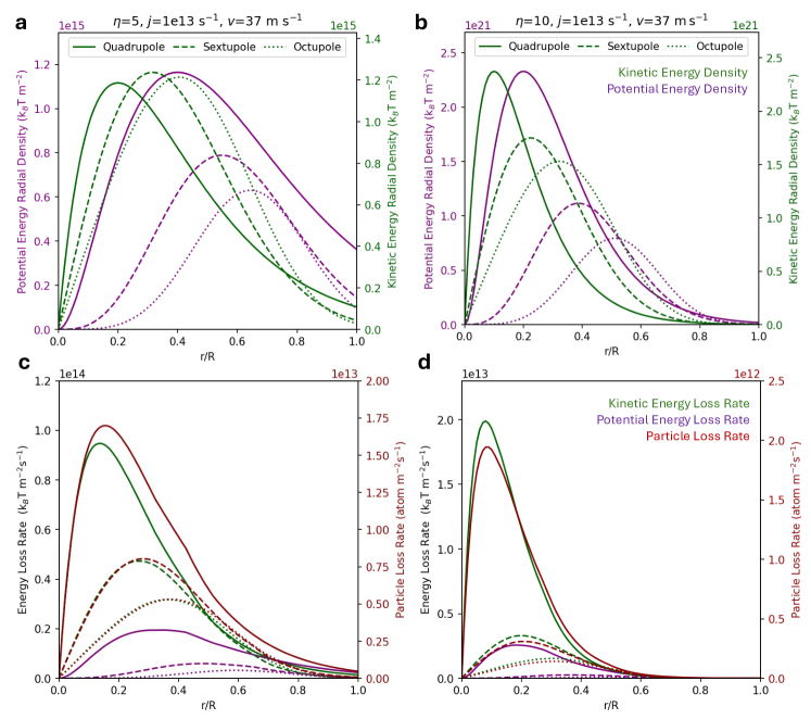
An example of a set of energy and particle loss rates for a given potential well depth and various multipolarities is given in Fig. 12 upper left, with the consequent temperature evolution in each case shown in Fig. 12, right. Dependencies on the input parameters are shown in the two additional panels.
For evaporation to be effective, the beam particles must maintain thermal contact with one another. This implies a constraint on the multipole radius and hence the beam radius, for a given throughput, velocity and multipolarity. To obtain this constraint, consider that the mean free path for a collision is given by
| (56) |
Most of the particles are contained within a radius determined by
| (57) |
In the regime we have many scatters per crossing of the guide, which corresponds to a fluid-like flow; cooling is unlikely to be efficient in such conditions, because particles scattering above the evaporation cut cannot efficiently leave the beam unless they happen to be on its periphery. On the other hand, if , the thermalization will be so slow that evaporation will not effectively cool the distribution. In one period of oscillation, each atom passes through about of path length, and we introduce the dimensionless parameter to quantify the opacity of the beam via . The ideal regime is expected to be in the regime , and as such we restrict our considerations to geometries that both require physically achievable values of and also allow for sufficient thermalization with .
| (58) |
If thermalization is not achieved, the highest energy particles will leave the guide but remaining particles will not then be up-scattered to replace them, effectively halting cooling. Assuming is maintained, we now have have two dynamical variables, and , whose evolution is governed by two equations of motion,
| (59) |
| (60) |
Numerical solution of these equations using the inputs described above provides cooling trajectories. Example trajectories for geometries of interest will be explored in Sec. III.
We note that our treatment in this section assumes both that all particles scattering above the energy cut will leave the guide, and that there are not other loss mechanisms actively removing particles with a non-trivial energy bias during transport. Neither of these assumptions is precisely true in practice. In fact, finite opacity of the beam implies that high energy particles could be rescattered before escaping; and also there are loss mechanisms active including dipole losses, Majorana spin flips, and collisions with recombined tritium gas that can perturb the ideal dynamics discussed here. While these are expected to be sub-leading effects, their impact will be assessed in more detail in future work.
II.5 Beam slowing via transverse perturbation
We now turn attention to slowing rather than cooling. In order to remove the mean momentum from the beam, we need to introduce some form of friction against the guide. Ignoring the effects of collisions, the trajectories of individual particles in a guide obey a simple equation of motion
| (61) |
For a straight multipole guide, the B field magnitude is
| (62) |
In this case, there is no force in the direction and so for each particle and hence for the whole ensemble is conserved (this could also be considered to be a consequence of Noether’s theorem, given the symmetry of the potential in ). In the special case where , i.e. for quadrupole guide, the and equations of motion are also decoupled, whereas for higher multipolarities they become coupled.
If we introduce perturbations to the linear guide such that it no longer has translational symmetry, will no longer necessarily be conserved and an ensemble of particles moving along the guide will experience friction and become slowed. On the other hand, in order to conserve energy this will also generate heat within the beam which must be removed by further evaporative cooling. We aim to exploit this behavior to slow as well as cool the beam of fast-moving atoms through evaporation.
A challenge in the analysis of the effect of complex magnetic geometry on the beam lies in defining an illustrative distribution function of particles entering it. If the guide has a complex profile then we may no longer rely on our previous notion of a thermalized co-moving ensemble within the guide, since the moving beam is explicitly out of thermal equilibrium with the z-dependent geometry, and will only achieve thermal equilibrium when it comes to rest with respect to the magnetic potential. We thus take inspiration from scattering theory. In a scattering problem, a well conditioned beam is impinged from spatial infinity on a localized potential, and the behavior of outgoing particles at infinity is studied. In analogy, for the present problem we will consider a long segment of straight multipole guide into which particles have thermalized as a co-moving distribution from ; then they will encounter a localized perturbation, and we will analyze the effect on the outgoing phase space distribution as . This is the expected situation if the beam has become well thermalized via interactions in a straight guide section before the perturbation, and any non-trivial kink in the magnetic geometry should thus be separated by such thermalizing sections. A more complex geometry can be constructed by applying a series of such perturbations and straight segments. For the moment we will ignore the effect of collisions since the effect of friction against the guide is approximately independent of how strongly the beam is interacting, though we will see shortly that the combined role of slowing and evaporation should be analyzed together, for a final workable geometry. We will also restrict attention in this section to quadrupole guides, since this allows for analysis in two dimensions rather than three.
As an example case, we will investigate scattering perturbations in the guide of the form
| (63) |
Continuity of the potential is ensured by boundary conditions The equation of motion in two dimensions is then
| (64) |
Any nontrivial function that satisfies the boundary conditions will generate a frictional slowing force on the beam, so even for this restricted form of perturbation a completely exhaustive survey of potential shapes is unfeasible. We will consider the following class of model where there is a single kink of controllable size dependent on free parameter .
| (65) |
In this case the equations of motion become
| (66) |
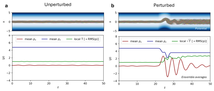
The ensemble behavior in a model with is compared against the unscattered scenario in Fig. 13. We see that at the point of the perturbation, the phase space distribution is disturbed, redistributing some bulk momentum from the direction into directions for each particle. Since each trajectory in the ensemble hits the scattering perturbation with a different phase, each emerges with a differently perturbed transverse momentum. This leads to expansion of the phase space distribution, resulting in an increase in temperature of the beam. This increase in temperature is accompanied by a reduction in the mean per particle. More dramatic perturbations also lead to reflections of particles back in the direction. The transverse momentum that is developed in the guide is damped as the various particles propagate with distinct wavelengths, eventually returning to , with reduced and increased internal temperature.
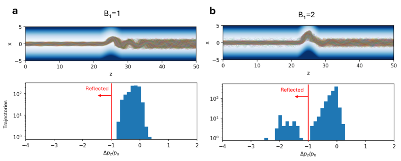
We can consider a slowing and cooling beamline as a sequence of slowing perturbations and cooling segments. Rather than stringing cooling and slowing components in series, it is conceivable that the two processes could be arranged to occur simultaneously at all positions. An important complication is that immediately after the kink, the phase space distribution is strongly pushed out of local thermal equilibrium; if the next kink follows too soon, we can find interference effects between them, which can lead to back scattering of particles upstream. This effect is also evident if any individual perturbation is made too large, as shown in the example of Fig. 14. A geometry whereby the perturbations are separated by straight segments of rethermalization in a linear section is one straightforward way to ensure the beam is well conditioned when entering each perturbation, to avoid backscattering effects. As such, we adopt this approach in the geometry outlined in Sec. III.
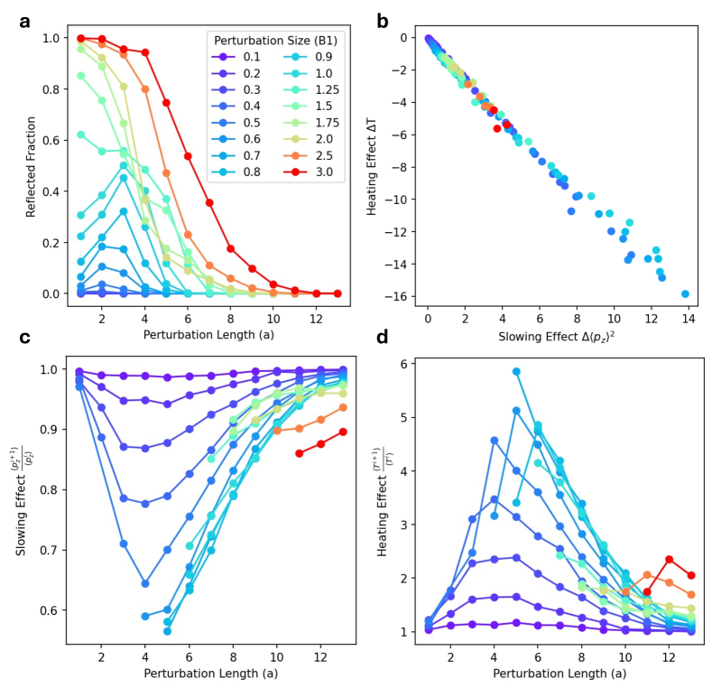
In summary, we can quantify the effect of a given guide perturbation on beam slowing using three figures of merit: 1) the change in temperature from before to after the kink, quantified via the root-mean-square of the transverse momentum RMS(); 2) the change in momentum from before to after the kink; 3) the fraction of reflected trajectories. These can be investigated as a function of the perturbation length (a) and magnitude () of Eq. 66. Plots showing the effects in these figures of merit in a series of calculated geometries using 10,000 simulated trajectories drawn from a distribution with are shown in Fig. 15, a,c,d, respectively. Fig. 15 (b) shows the correlation between the slowing and cooling effects, showing they are directly linearly related, as should be expected - while scattering from the potential perturbation does not conserve momentum, it must conserve energy, and all the energy lost from the mean beam momentum must be absorbed into the internal motion of the particles. That the points on Fig 15 (b) do not fall exactly on a straight line reflects that the distribution emerging from the kink is not a perfect Maxwell Boltzmann distribution, as it will only assume this form after rethermalization through collisions.
Several further conclusions can be drawn from consideration of the dependence of the slowing efficiency on perturbation parameters shown in Fig 15. First, as the perturbation becomes very long, both the slowing / heating effects and reflection probabilities tend to zero; in this case the perturbation simply becomes an adiabatic curve to the guide that particles will follow without their trajectories being significantly interrupted. The cooling effect and reflection probabilities also tend to zero as , expected since this is a limit in which the perturbation vanishes entirely. Next, we note that for a given perturbation size there is a minimal length such that it does not create a significant particle reflection effect. Any configuration with a large reflected fraction is not useful for our purposes since those particles will return and interact with the oncoming beam; but it also makes the other two variables quantifying heat and momentum of the still-propagating part of the distribution rather less easy to interpret, since they now apply to only a subset of the current and so the net effect of cooling or slowing becomes obscured by the velocity-dependence of the reflectivity. As such, we have opted only to plot the points in top right and the bottom left and right panels of Fig 15 that have a small reflection probability (<2% for these plots, though in practice most of these points do not show any reflected trajectories).
Based on these studies, the optimal cooling effect occurs around and , giving a 60% slowing and factor of 3 reheating. These optima are found to depend somewhat on the z momentum of the beam entering the perturbation, though in the range which will be relevant to our design, only a small dependence to the slowing and heating effect is observed, so we will take these operating parameters as a baseline for subsequent calculations.
III MECB geometry for the Li pathfinder beam
The cooling geometry proposed here anticipates a flux emerging from an upstream element, for the case of Li a partially cooled beam from a hot oven followed by a resonant Zeeman slower [27, 28, 29, 61], that will have a mean energy significantly above the trapping strength of the strongest available magnets. The first part of the beamline is thus considered to be a “catcher”, which essentially extracts the bottom part of the Maxwell Boltzmann distribution that can be trapped. No cooling happens in this section, and the beam density is deliberately kept low until the hot atoms have escaped by using a large diameter, high multipolarity segment.
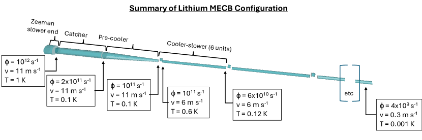
Once the hot atoms have left the distribution after approximately one meter of catcher section the beam is then brought into a condition whereby evaporative cooling is effective. This means tuning the magnetic geometry such that the thermalization parameter in the catcher section becomes in the evaporative cooling sections. The first stage of MECB cooling then uses the strongest available magnets until their cooling effect is saturated and the current and temperature stabilize. By the end of this segment the beam is well conditioned into a moving but thermalized Maxwell Boltzmann distribution.
The remainder of the beamline after the pre-cooler is multiple meters long and is arranged as a series of slowing and cooling units, which evaporatively cools the beam to the required 1 mK and slows the distribution to a low speed such that it can be injected into a trap. Avoiding zero velocity is important, as otherwise the atoms do not travel further along the beamline; as such in designing the desired cooling trajectories we have been careful to maintain . The design shown here keeps this mass flow number between 3 and 5, though modifications may be made to this balance based on observed performance in prototypes. In the Li test system, the beam is probed to measure its current and temperature at an end station and assess the effectiveness of the MECB design. A sketch of this beamline concept is shown in Fig. 16. In the ultimate T beamline as sketched in Sec. IV, a subsequent stage of beamline will be needed to turn the beam vertically and have it enter the magneto-gravitational trap.
III.1 Catcher
The goal of this segment is to trap as large a fraction of the current emerging from the Zeeman slower system as possible, simply by selecting the relevant low energy part of Maxwell-Boltzmann distribution with the strongest possible trapping magnets. The density in this section is deliberately kept low, in order to avoid re-thermalization while the fastest transverse particles leave the beam. Past Zeeman slowers [62] have produced outgoing currents of per second at the oven and per second at the Zeeman slower exit. The Project 8 Li test source has a much larger oven aperture than these past devices and so we expect to be able to achieve larger currents by one to two orders of magnitude. As such, for the following calculations we assume the incoming current to the MECB stage to be , at a pre-cooled temperature of 1 K. For a transverse cut at , the surviving particle fraction is then
| (67) |
and the remaining energy fraction is
| (68) |
Equipartition tells us the temperature scales as , which means that following this cut the remainder of the distribution rethermalizes and we will have a temperature of
| (69) |
If we are taking a small bite out of the bottom end of the distribution, it is appropriate to Taylor expand these expressions at small to find we will keep a particle fraction and temperature fraction of the original following
| (70) |
The strongest available permanent magnets that we are aware of have T, implying at the top end in a simple multipole geometry, giving an effective temperature of 0.1 K and current of . Notably, Halbach geometries may allow for enhancement of this surface field strength, though at the cost of additional magnetic elements that would enhance the difficulty of removing recombined T2 from the beamline. Since only forward-going particles will enter the catcher, the forward velocity of this ensemble will correspond to the mean Maxwell Boltzmann velocity of 11 .
III.2 Pre-cooler
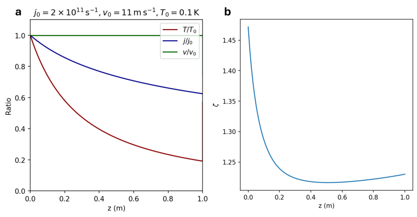
To begin true evaporative cooling this must be compressed into a thermalization radius of around 1 cm for . The catcher is an initial section of length 1 m with high multipolarity and a large diameter to bite off the trappable flux; this must be followed by a section that conditions the trapped ensemble into a beam with density sufficiently high for evaporative cooling. This can be accomplished via an octupole guide of steadily reducing diameter, guiding the current into a 1 m long straight octupole segment. We have considered here an octupole with radius steadily decreasing from 3 cm to 1 cm, which provides sufficient space to insert the appropriate bar magnets but condenses the beam as much as possible given the available B field strengths. This segment also provides the first stage of evaporative cooling and conditions the beam for the subsequent more aggressive slower-cooler section. For the purposes of this study, we assume that the beam has become thermalized upon entering this section, though in practice this may be partially occurring during the upstream section of the pre-cooler without significant changes to our predictions.
The evaporative cooling rates in the pre-cooler are calculated in Fig. 17, a. We see the current will stabilize in a T guide after around 1 m with around 60% of the incoming current and 20% of the original temperature, given an incoming beam with the properties predicted above. The value of in this section can be calculated as,
| (71) |
The geometry chosen here maintains all the way along the pre-cooler, ensuring both efficient thermalization and effective evaporative dynamics.
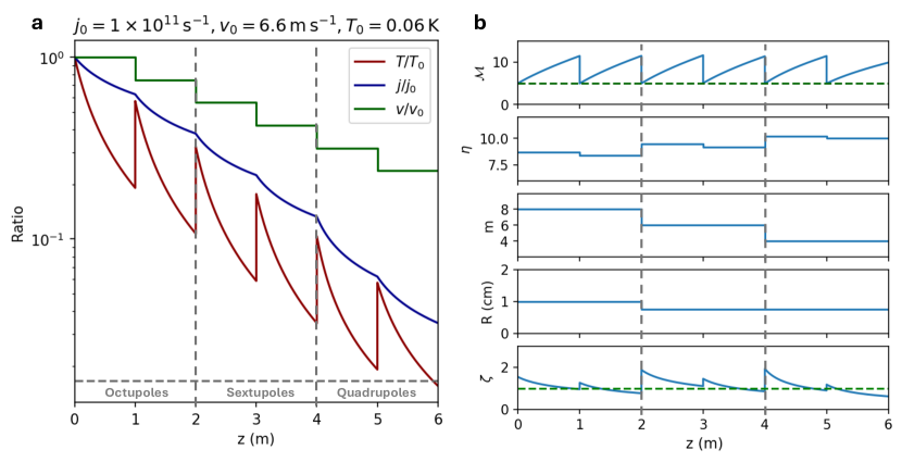
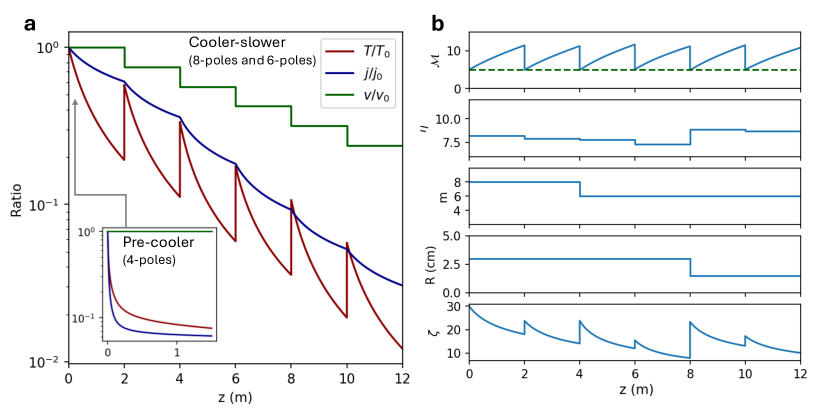
III.3 Cooler-slower
At the end of the pre-cooler we expect , and . The calculations of section II.5 are in temperature scaled units, so will apply in any scenario where we have input current with . With such an incoming current, a slower segment can be implemented which preserves the total current, reduces central momentum by a factor of and increases temperature by a factor of . Since the slowing effect itself does not rely on collisions, that analysis applies for any current density. The temperature can then be reduced using a segment of evaporative cooling at constant to return to the original mass flow number. The goal of our design will thus be to achieve at the entrance to each slowing element , while evaporatively cooling in segments with in between. This is accomplished in the following set of repeating steps:
-
1.
Slowing section with momentum change accompanied by reheating of ,
-
2.
Cooling section to return to with temperature change and momentum change
The combined effect of these two elements is and , and the sequence always maintains at least 3 times the central momentum relative to temperature to keep the beam moving forward along the beamline. The choice to slow first rather than cool first serves to minimize the total length of the beamline, and improve thermalization in the cooling sections.
To accomplish the goal of cooling from to we will need segments. We have 7 m of laboratory real estate available for the test beam, so we arbitrarily pick as a design driver that each will be 0.5 m in length. The values of , and for each segment are chosen to maintain as well as possible at order-1, while cooling with the required power in 1 m of distance, though notably becomes larger than one at the downstream end where the beam is cold, dense, and slow. Because the beam is so slow in this region, an reduced ability for scattered particles to leave the beam is not known to compromise the evaporative cooling efficiency, since they will have many opportunities to do so during the 1 m segment length, unlike near the top end, where maintaining is crucial.
We predict that the proposed configuration will achieve a beam with final temperature at 1 mK with longitudinal momentum of 5 mK at 4% efficiency in the slower-cooler section. The operating parameters of the system as well as its performance in terms of and is shown in Fig. 18, left. A more efficient beam could also be produced with longer segments and slower cooling if desired, though the beamline length would be longer for reaching the same target temperature. This system will allow for investigation of the MECB cooling and slowing dynamics, in order to prepare a detailed design for an atomic T cooling beam.
Several salient features of the MECB concept are visible in the detailed parameter trajectories of Fig. 18, b. First, we see that the transition from higher multipoles to lower ones, as well as reducing the multipole diameter along the beam line, is required to keep as the beam current is reduced. This results in an accompanying decrease of cooling efficiency since higher multipoles maintain a larger cooling exponent . The trade-off between these factors, as well as practical considerations such as maintaining multipole diameters at practical scales, dictates the range of possible configurations for an effective MECB system. We have fixed the initial atom current in these calculations to values similar to those demonstrated in past experiments with Zeeman slowers. If higher incoming currents were achievable, higher multipoles would remain viable for the downstream sections, avoiding the largest losses and increasing efficiency. This example shows one possible set of parameters for cooling a 6Li beam, though clearly there is significant flexibility to adjust multipolarity , radii , evaporation cut , and segment lengths, all in continuous and distance-dependent ways, as well as slowing power per segment and modularity of the cooling/slowing steps. The system is thus highly tunable with many degrees of freedom that can be traded off and optimized within the constraints imposed by considerations associated with realization of a practical geometry.
IV Magnetic geometry for T cooling and slowing
For the eventual T beamline, the scattering cross sections are smaller, but the currents and velocities are higher than the lithium test system. This both affects the dynamics of the evaporative cooling, and requires a commensurately longer beamline. There are also important considerations that the present analysis neglects, which will be important for proper design of the T system, including interaction with recombined background gas, and the momentum dependence of the T triplet scattering cross section. Nevertheless, here we use the methods of the above section to outline a rough scheme for the T cooling system.
Project 8 projections to date suggest that between 1014 and 1016 atoms per second must be delivered to the magnetic trap at mK temperatures in order to conduct a sensitive neutrino mass search. We thus consider here a target current of 1015 s-1 and target temperature of 1 mK as a representative benchmark. The MECB line is only one of many elements that must be developed to supply cold atomic T for Project 8. A sketch of the anticipated scheme is shown in Fig. 19. The losses associated with cracking, accommodation, dissociation and capture into the beamline are all substantial and carry large uncertainties. For present purposes we consider that a suitable current of 5 atoms per second will be available entering the MECB section, deferring upstream tritium source considerations for future work. It should be emphasized that the design discussed here is speculative, and the final design is expected to be informed by intervening R&D, further simulation studies, and the lithium test beam apparatus.
As in the lithium system, the upper end of the magnetic cooling beamline segment for T is limited by the strength of the strongest obtainable permanent magnets, currently estimated as T. In a Halbach configuration, surface fields of 0.8 T can be reached [63]. Despite the apparent opportunities to reach higher trapping fields, the primary design-driving concern at the top end of the beamline is the capability to remove recombined and warm T2 molecules from the guide. This appears to restrict the upper segments to be simple permanent quadrupole magnets, despite the performance penalty implied in terms of trapping and cooling power. Still higher fields could potentially be obtained with superconducting magnets. These are not considered in the default design on the grounds of cost and complexity, though they could be explored in future investigations.
The top end of the beamline will serve as a ‘capture’ section to extract the trappable subset of the atoms from a hotter beam emerging from the accommodator at 10-30 K. The design of this segment remains under development, with various magnetic or mechanical geometries under consideration, some of which would produce a distinctly non-effusive current. Magnetic evaporative cooling begins with an effective temperature of 0.2 K and current of s-1. A pre-cooler section, restricted to quadrupoles for vacuum pumping purposes and using the largest available surface field permanent magnets (estimated here as Bmax=0.5 T), conditions the beam for slowing and cooling. We assume the bulk velocity of the distribution entering the catcher corresponds to effusive flow at 1 K, which implies a velocity of . These are speculative baseline assumptions, to be met with data from test systems and more detailed calculations concerning the upstream elements of the Project 8 atomic T R&D program.
Both because it is important to pump out recombined T2 gas and because maintaining for thermalization is a far less pressing concern in the high current environment of the T beam than in the previous example, we use larger multipole radii in the T beam than were used in the Li geometry. The pre-cooler in this case reduces the multipole radius from 6 cm at the interface to the capture section to 3 cm in the upper aperture of the cooler-slower, which then uses 3 cm radii multipoles at the top end and 2 cm at the downstream one. Over 12 m it seems to be plausible to cool the distribution to 1 mK with efficiency with a number of different schemes, using realistic parameters and assuming the T triplet scattering cross sections outlined in Sec. II.3, given an initial current of 5s-1 at 200 mK. One example geometry and its associated performance parameters is given in Fig. 20. In this geometry, is maintained at close to 20 along the beamline, which is sufficient to thermalize the beam but not so large as to completely inhibit evaporation due to beam opacity. The mass flow number is returned to following each cooling/slowing sector, using a similar scheme to that used in Sec. III. The ultimate current emerging from this design is around s-1 at 0.3 mK.
A detailed engineering design for the Project 8 MECB system, as well as a truly robust performance estimate, will require consideration of a number of other factors, including tritium handling, evacuation of warm gas from the beam, understanding of Majorana spin-flip losses in the beam, energy- and magnetic-field dependent cross sections, detailed treatment of position-dependent beam opacity, and dipole losses from d-state collisions, among others. Nevertheless, based on these early studies, it appears there are realistic possibilities to use the MECB method as a central component of the Project 8 cold atomic tritium source.
V Conclusions
MECB is a technique for achieving cold beams of magnetically trappable atoms in a laser-less configuration. The Project 8 collaboration is developing this method to provide a well-conditioned, cooled and slowed beam of atomic T to feed the Project 8 magneto-gravitational trap. The method is being experimentally probed via an initial Li test-beam phase.
The dynamics of MECB can be understood on the basis of thermalization and evaporation of a trapped, self-interacting atomic vapor. A slowing component can be added via perturbations whose form is controlled by the requirement that they not reflect a substantial component of the beam, separated by cooling segments to remove the heat that is generated by the slowing process.
We have presented in this paper a suite of analytic and numerical calculations developed to estimate the performance of MECB cooling and slowing in geometries conceived for cooling of both Li and T systems. Our results suggest that the required currents of 1014 s-1-1016 s-1 of T at temperatures of order 1 mK may be deliverable to the Project 8 trap using the MECB approach as long as upstream elements provide a tritium current of s-1 at 200 mK. The ongoing atomic T R&D program of Project 8 and its Li pathfinder phase will confront these estimates with data in the near future. Proof of successful MECB-based slowing and cooling will be an important step toward a direct neutrino mass measurement based on trapped atomic T, further advancing the frontier of neutrino mass sensitivity toward the lower limit associated with the inverted neutrino mass ordering.
Acknowledgments
This material is based upon work supported by the following sources: the U.S. Department of Energy Office of Science, Office of Nuclear Physics, under Award No. DE-SC0020433 to Case Western Reserve University (CWRU), under Award No. DE-SC0011091 to the Massachusetts Institute of Technology (MIT), under Field Work Proposal Number 73006 at the Pacific Northwest National Laboratory (PNNL), a multiprogram national laboratory operated by Battelle for the U.S. Department of Energy under Contract No. DE-AC05-76RL01830, under Early Career Award No. DE-SC0019088 to Pennsylvania State University, under Award No. DE-SC0024434 to the University of Texas at Arlington, under Award No. DE-FG02-97ER41020 to the University of Washington, and under Award No. DE-SC0012654 to Yale University; the National Science Foundation under Grant No. PHY-2209530 to Indiana University, and under Grant No. PHY-2110569 to MIT; the Karlsruhe Institute of Technology (KIT) Center Elementary Particle and Astroparticle Physics (KCETA); Laboratory Directed Research and Development (LDRD) 18-ERD-028 and 20-LW-056 at Lawrence Livermore National Laboratory (LLNL), prepared by LLNL under Contract DE-AC52-07NA27344, LLNL-JRNL-871979; the LDRD Program at PNNL; Yale University; and the Cluster of Excellence "Precision Physics, Fundamental Interactions, and Structure of Matter" (PRISMA+ EXC 2118/1) funded by the German Research Foundation (DFG) within the German Excellence Strategy (Project ID 39083149).
Appendix A: Numerical solution of the Boltzmann collision integral for cooling rates
The time derivative of the phase space density required to calculate evaporative cooling rates can be evaluated via the full collisional Boltzmann transport equation. This equation has the full form
| (72) |
where the terms represent, from left to right: time evolution of phase space, mass flow due to inertia, force from applied potential, and collision integral that leads to thermalization. For spherical collisions with constant cross section, can be written as
| (73) |
| (74) |
Inside the square brackets and are treated as fixed, and we can rewrite the and integrals as
| (75) |
| (76) |
The momentum conserving delta function fixes the center of mass momentum before and after, as :
| (77) |
The energy conserving delta function fixes the magnitude of , but its angle is free,
| (78) |
Manipulating the energy delta function we find the dependence drops out (as expected from kinematics in the center of mass frame) so
| (79) |
We find that and we have to integrate over directions. Continuing with the Boltzmann equation,
| (80) | |||||
The two delta functions eliminate the freedom in and , leaving only the solid angle integral for ,
| (81) |
Where “constrained” means we must only evaluate at kinematically valid points, defined by
| (82) |
We evaluate the final integrals by Monte Carlo integration over the phase space distribution. Sampling points in and solid angle of with from phase space volume , the appropriate discrete approximation to the integral is
| (83) |
If our phase space runs from for , and the phase space volume associated with solid angle is . Thus, sampling values for and from these ranges,
| (84) |
The collision integral will also be cylindrically symmetric, so
| (85) |
In principle we can re-evaluate for any phase space distribution. However, simple scaling arguments can be made that show that for a distribution which is close in form to the Maxwell Boltzmann, the collision terms have expected scaling with of
| (86) |
This scaling is validated using our numerical code, with results shown in Fig. 21, and the agreement is excellent. It thus suffices to numerically evaluate and at a representative and at each , then map to each other value with the above scaling laws. From this information we can explore the loss rates of energy and particles geometrically across a multipole guide.
Appendix B: Table of variable names
| Symbol | Meaning |
|---|---|
| Position | |
| Momentum | |
| Particle mass | |
| Boltzmann constant | |
| Temperature | |
| Cooling exponent | |
| Scattering cross section | |
| Scattering mean free path | |
| Collisions per beam crossing | |
| Dimensionality of trap | d |
| Multipolarity | m |
| Potential power law | |
| Mass flow number | |
| Phase space function | |
| Density | |
| Total particle number | |
| Energy | |
| Scaled energy () | |
| Density of energy states | |
| Beam longitudinal momentum | |
| Evaporative heat loss | |
| Equipartition constant | |
| Logarithmic cooling rates (energy, number) | |
| Fraction of (energy, number), that are (above, below) cut | |
| Evaporation cut (in units of ) | |
| Excess energy loss per particle in evaporation | |
| Momentum at evaporation cut | |
| Magnetic field | |
| Maximum B field at surface | |
| Multipole segmentation correction to B field | |
| Radial position | r |
| Beam bulk velocity | |
| Flux (particles per second through a surface) | |
| Radius of multipole | |
| Radius in which majority of particles are contained | |
| Total Energy | E |
| Trapping potential | V |
| Slowing perturbation parameters | a, |
References
- [1] M. Aker et al., “The design, construction, and commissioning of the KATRIN experiment,” Journal of Instrumentation, vol. 16, p. T08015, aug 2021.
- [2] M. Aker, D. Batzler, A. Beglarian, J. Behrens, J. Beisenkötter, M. Biassoni, B. Bieringer, Y. Biondi, F. Block, S. Bobien, et al., “Direct neutrino-mass measurement based on 259 days of katrin data,” arXiv preprint arXiv:2406.13516, 2024.
- [3] N. Aghanim et al., “Planck 2018 results. VI. Cosmological parameters,” Astron. Astrophys., vol. 641, p. A6, 2020.
- [4] M. J. Dolinski, A. W. Poon, and W. Rodejohann, “Neutrinoless double-beta decay: status and prospects,” Annual Review of Nuclear and Particle Science, vol. 69, pp. 219–251, 2019.
- [5] M. C. Gonzalez-Garcia, M. Maltoni, and T. Schwetz, “Nufit: three-flavour global analyses of neutrino oscillation experiments,” Universe, vol. 7, no. 12, p. 459, 2021.
- [6] R. L. Workman and Others, “Review of Particle Physics,” PTEP, vol. 2022, p. 083C01, 2022.
- [7] B. Monreal and J. Formaggio, “Relativistic Cyclotron Radiation Detection of Tritium Decay Electrons as a New Technique for Measuring the Neutrino Mass,” Phys. Rev., vol. D80, p. 051301, 2009.
- [8] A. Ashtari Esfahani et al., “Determining the neutrino mass with cyclotron radiation emission spectroscopy—Project 8,” J. Phys. G, vol. 44, no. 5, p. 054004, 2017.
- [9] A. Ashtari Esfahani et al., “Tritium Beta Spectrum Measurement and Neutrino Mass Limit from Cyclotron Radiation Emission Spectroscopy,” Phys. Rev. Lett., vol. 131, no. 10, p. 102502, 2023.
- [10] A. Ashtari Esfahani, S. Böser, N. Buzinsky, M. C. Carmona-Benitez, C. Claessens, L. de Viveiros, P. J. Doe, M. Fertl, J. A. Formaggio, J. K. Gaison, L. Gladstone, M. Guigue, J. Hartse, K. M. Heeger, X. Huyan, A. M. Jones, K. Kazkaz, B. H. LaRoque, M. Li, A. Lindman, E. Machado, A. Marsteller, C. Matthé, R. Mohiuddin, B. Monreal, R. Mueller, J. A. Nikkel, E. Novitski, N. S. Oblath, J. I. Peña, W. Pettus, R. Reimann, R. G. H. Robertson, D. Rosa De Jesús, G. Rybka, L. Saldaña, M. Schram, P. L. Slocum, J. Stachurska, Y.-H. Sun, P. T. Surukuchi, J. R. Tedeschi, A. B. Telles, F. Thomas, M. Thomas, L. A. Thorne, T. Thümmler, L. Tvrznikova, W. Van De Pontseele, B. A. VanDevender, J. Weintroub, T. E. Weiss, T. Wendler, A. Young, E. Zayas, and A. Ziegler, “Cyclotron radiation emission spectroscopy of electrons from tritium decay and internal conversion,” Phys. Rev. C, vol. 109, p. 035503, Mar 2024.
- [11] L. I. Bodine, D. S. Parno, and R. G. H. Robertson, “Assessment of molecular effects on neutrino mass measurements from tritium decay,” Phys. Rev. C, vol. 91, p. 035505, Mar 2015.
- [12] A. Serebrov, V. Varlamov, A. Kharitonov, A. Fomin, Y. Pokotilovski, P. Geltenbort, J. Butterworth, I. Krasnoschekova, M. Lasakov, R. Tal’Daev, et al., “Measurement of the neutron lifetime using a gravitational trap and a low-temperature fomblin coating,” Physics Letters B, vol. 605, no. 1-2, pp. 72–78, 2005.
- [13] P. Walstrom, J. Bowman, S. Penttila, C. Morris, and A. Saunders, “A magneto-gravitational trap for absolute measurement of the ultra-cold neutron lifetime,” Nuclear Instruments and Methods in Physics Research Section A: Accelerators, Spectrometers, Detectors and Associated Equipment, vol. 599, no. 1, pp. 82–92, 2009.
- [14] R. Pattie Jr, N. Callahan, C. Cude-Woods, E. Adamek, L. J. Broussard, S. Clayton, S. Currie, E. Dees, X. Ding, E. Engel, et al., “Measurement of the neutron lifetime using a magneto-gravitational trap and in situ detection,” Science, vol. 360, no. 6389, pp. 627–632, 2018.
- [15] A. Serebrov, E. Kolomensky, A. Fomin, I. Krasnoshchekova, A. Vassiljev, D. Prudnikov, I. Shoka, A. Chechkin, M. Chaikovskiy, V. Varlamov, et al., “Neutron lifetime measurements with a large gravitational trap for ultracold neutrons,” Physical Review C, vol. 97, no. 5, p. 055503, 2018.
- [16] K. Tschersich and V. Von Bonin, “Formation of an atomic hydrogen beam by a hot capillary,” Journal of applied physics, vol. 84, no. 8, pp. 4065–4070, 1998.
- [17] S. Aleiferis, P. Svarnas, S. Béchu, O. Tarvainen, and M. Bacal, “Production of hydrogen negative ions in an ecr volume source: balance between vibrational excitation and ionization,” Plasma Sources Science and Technology, vol. 27, no. 7, p. 075015, 2018.
- [18] I. F. Silvera and J. Walraven, “The stabilization of atomic hydrogen,” Scientific American, vol. 246, no. 1, pp. 66–76, 1982.
- [19] R. Guyer and M. Miller, “Interaction of Atomic Hydrogen with the Surface of He-4,” Physical Review Letters, vol. 42, no. 26, pp. 1754–1757, 1979.
- [20] H. F. Hess, “Evaporative cooling of magnetically trapped and compressed spin-polarized hydrogen,” Physical Review B, vol. 34, no. 5, p. 3476, 1986.
- [21] N. Masuhara, J. M. Doyle, J. C. Sandberg, D. Kleppner, T. J. Greytak, H. F. Hess, and G. P. Kochanski, “Evaporative cooling of spin-polarized atomic hydrogen,” Physical Review Letters, vol. 61, no. 8, p. 935, 1988.
- [22] D. G. Fried, T. C. Killian, L. Willmann, D. Landhuis, S. C. Moss, D. Kleppner, and T. J. Greytak, “Bose-einstein condensation of atomic hydrogen,” Physical Review Letters, vol. 81, no. 18, p. 3811, 1998.
- [23] D. G. Fried, “Bose-einstein condensation of atomic hydrogen,” 1999.
- [24] W. Ketterle and N. Van Druten, “Evaporative cooling of trapped atoms,” in Advances in atomic, molecular, and optical physics, vol. 37, pp. 181–236, Elsevier, 1996.
- [25] T. Lahaye, Z. Wang, G. Reinaudi, S. Rath, J. Dalibard, and D. Guéry-Odelin, “Evaporative cooling of a guided rubidium atomic beam,” Physical Review A, vol. 72, no. 3, p. 033411, 2005.
- [26] E. Mandonnet, A. Minguzzi, R. Dum, I. Carusotto, Y. Castin, and J. Dalibard, “Evaporative cooling of an atomic beam,” The European Physical Journal D-Atomic, Molecular, Optical and Plasma Physics, vol. 10, pp. 9–18, 2000.
- [27] W. Bowden, W. Gunton, M. Semczuk, K. Dare, and K. W. Madison, “An adaptable dual species effusive source and zeeman slower design demonstrated with rb and li,” Review of Scientific Instruments, vol. 87, no. 4, p. 043111, 2016.
- [28] D. Garwood, L. Liu, J. Mongkolkiattichai, J. Yang, and P. Schauss, “A hybrid zeeman slower for lithium,” Review of Scientific Instruments, vol. 93, no. 3, p. 033202, 2022.
- [29] G. E. Marti, R. Olf, E. Vogt, A. Öttl, and D. M. Stamper-Kurn, “Two-element zeeman slower for rubidium and lithium,” Physical Review A, vol. 81, no. 4, p. 043424, 2010.
- [30] S. Chervenkov, X. Wu, J. Bayerl, A. Rohlfes, T. Gantner, M. Zeppenfeld, and G. Rempe, “Continuous Centrifuge Decelerator for Polar Molecules ,” Phys. Rev. Lett., vol. 112, p. 013001, 2014.
- [31] S. D. Hogan, D. Sprecher, M. Andrist, N. Vanhaecke, and F. Merkt, “Zeeman deceleration of h and d,” Physical Review A- Atomic, Molecular, and Optical Physics, vol. 76, no. 2, p. 023412, 2007.
- [32] A. Libson, S. T. Bannerman, R. J. Clark, T. R. Mazur, and M. G. Raizen, “The atomic coilgun and single-photon cooling: A method for trapping and cooling of hydrogen isotopes,” Hyperfine Interactions, vol. 212, pp. 203–212, 2012.
- [33] U. Schünemann, H. Engler, M. Zielonkowski, M. Weidemüller, and R. Grimm, “Magneto-optic trapping of lithium using semiconductor lasers,” Optics Communications, vol. 158, no. 1-6, pp. 263–272, 1998.
- [34] A. Mosk, S. Jochim, H. Moritz, T. Elsässer, M. Weidemüller, and R. Grimm, “Resonator-enhanced optical dipole trap for fermionic lithium atoms,” Optics Letters, vol. 26, no. 23, pp. 1837–1839, 2001.
- [35] A. Mosk, S. Kraft, M. Mudrich, K. Singer, W. Wohlleben, R. Grimm, and M. Weidemüller, “Mixture of ultracold lithium and cesium atoms in an optical dipole trap,” Applied Physics B, vol. 73, pp. 791–799, 2001.
- [36] T. Tiecke, S. Gensemer, A. Ludewig, and J. Walraven, “High-flux two-dimensional magneto-optical-trap source for cold lithium atoms,” Physical Review A – Atomic, Molecular, and Optical Physics, vol. 80, no. 1, p. 013409, 2009.
- [37] V. A. Vinogradov, K. A. Karpov, S. S. Lukashov, and A. V. Turlapov, “Trapping of lithium atoms in a large hollow optical dipole trap,” Quantum Electronics, vol. 50, no. 6, p. 520, 2020.
- [38] A. Lagendijk, I. F. Silvera, and B. J. Verhaar, “Spin exchange and dipolar relaxation rates in atomic hydrogen: Lifetimes in magnetic traps,” Physical Review B, vol. 33, no. 1, p. 626, 1986.
- [39] T. Kato, “On the adiabatic theorem of quantum mechanics,” Journal of the Physical Society of Japan, vol. 5, no. 6, pp. 435–439, 1950.
- [40] P. Blümler and H. Soltner, “Practical concepts for design, construction and application of halbach magnets in magnetic resonance,” Applied Magnetic Resonance, vol. 54, no. 11, pp. 1701–1739, 2023.
- [41] M. Ioffe, “Mirror traps,” in Lectures presented at the Trieste Seminar on Plasma Physics, p. 421, 1965.
- [42] A. Wolski, “Maxwell’s equations for magnets,” arXiv preprint arXiv:1103.0713, 2011.
- [43] K. B. Davis, M. O. Mewes, and W. Ketterle, “An analytical model for evaporative cooling of atoms,” Applied Physics B, vol. 60, pp. 155–159, 1995.
- [44] A. Sandouqa and B. Joudeh, “The thermophysical properties of spin-polarized atomic tritium (t) in the temperature range 0.01 k–10 k,” Physica Scripta, vol. 93, no. 9, p. 095401, 2018.
- [45] I. F. Silvera, “The solid molecular hydrogens in the condensed phase: Fundamentals and static properties,” Reviews of Modern Physics, vol. 52, no. 2, p. 393, 1980.
- [46] W. Kołos and L. Wolniewicz, “Improved potential energy curve and vibrational energies for the electronic ground state of the hydrogen molecule,” Journal of molecular spectroscopy, vol. 54, no. 2, pp. 303–311, 1975.
- [47] J. Dugan Jr and R. Etters, “Ground state properties of spin-aligned atomic hydrogen,” The Journal of Chemical Physics, vol. 59, no. 11, pp. 6171–6172, 1973.
- [48] M. Jamieson, A. Dalgarno, B. Zygelman, P. Krstić, and D. R. Schultz, “Collisions of ground-state hydrogen atoms,” Physical Review A, vol. 61, no. 1, p. 014701, 1999.
- [49] D. Blume, B. Esry, C. H. Greene, N. Klausen, and G. Hanna, “Formation of atomic tritium clusters and Bose-Einstein condensates,” Physical Review Letters, vol. 89, no. 16, p. 163402, 2002.
- [50] B. Joudeh, “Scattering properties of ground-state spin-polarized atomic hydrogen,” Physica B: Condensed Matter, vol. 421, pp. 41–45, 2013.
- [51] W. C. Stwalley, “Collisions and reactions of ultracold molecules,” Canadian journal of chemistry, vol. 82, no. 6, pp. 709–712, 2004.
- [52] A. Berlinsky, “Elementary scattering processes in a low temperature atomic hydrogen gas,” Le Journal de Physique Colloques, vol. 41, no. C7, pp. C7–43, 1980.
- [53] A. Al-Maaitah, “Scattering properties of spin-polarized atomic tritium,” European Scientific Journal, vol. 8, no. 24, 2012.
- [54] E. Abraham, W. McAlexander, J. Gerton, R. Hulet, R. Côté, and A. Dalgarno, “Triplet s-wave resonance in Li 6 collisions and scattering lengths of Li 6 and Li 7,” Physical Review A, vol. 55, no. 5, p. R3299, 1997.
- [55] K. M. O’Hara, Optical trapping and evaporative cooling of fermionic atoms. PhD thesis, Duke University, 2000.
- [56] D. D. Konowalow and M. L. Olson, “The electronic structure and spectra of the X 1+ g and A 1+ u states of Li2,” The Journal of Chemical Physics, vol. 71, no. 1, pp. 450–457, 1979.
- [57] D. D. Konowalow, R. M. Regan, and M. E. Rosenkrantz, “The “most likely”potential energy curve for the lowest 3+ u state of li2,” The Journal of chemical physics, vol. 81, no. 10, pp. 4534–4536, 1984.
- [58] I. Schmidt-Mink, W. Müller, and W. Meyer, “Ground-and excited-state properties of li2 and li2+ from ab initio calculations with effective core polarization potentials,” Chemical physics, vol. 92, no. 2-3, pp. 263–285, 1985.
- [59] Z.-C. Yan, J. F. Babb, A. Dalgarno, and G. Drake, “Variational calculations of dispersion coefficients for interactions among H, He, and Li atoms,” Physical Review A, vol. 54, no. 4, p. 2824, 1996.
- [60] W. T. Zemke and W. C. Stwalley, “Analysis of long-range dispersion and exchange interactions of two lithium atoms,” The Journal of Physical Chemistry, vol. 97, no. 10, pp. 2053–2058, 1993.
- [61] N. Vanhaecke, U. Meier, M. Andrist, B. H. Meier, and F. Merkt, “Multistage zeeman deceleration of hydrogen atoms,” Physical Review A, vol. 75, no. 3, p. 031402, 2007.
- [62] J. O. Stack, An ultra-cold lithium source for investigating cold dipolar gases. PhD thesis, Imperial College London, 2011.
- [63] D. Salvat, “New results from the ucn experiment,” Bulletin of the American Physical Society, vol. 65, 2020.