Optimal Coupled Sensor Placement and Path-Planning in Unknown Time -Varying Environments

Abstract

We address path-planning for a mobile agent to navigate in an unknown environment with minimum exposure to a spatially and temporally varying threat field. The threat field is estimated using pointwise noisy measurements from a mobile sensor network. For this problem, we present a new information gain measure for optimal sensor placement that quantifies reduction in uncertainty in the path cost rather than the environment state. This measure, which we call the context-relevant mutual information (CRMI), couples the sensor placement and path-planning problem. We propose an iterative coupled sensor configuration and path-planning (CSCP) algorithm. At each iteration, this algorithm places sensors to maximize CRMI, updates the threat estimate using new measurements, and recalculates the path with minimum expected exposure to the threat. The iterations converge when the path cost variance, which is an indicator of risk, reduces below a desired threshold. We show that CRMI is submodular, and therefore, greedy optimization provides near-optimal sensor placements while maintaining computational efficiency of the CSCP algorithm. Distance-based sensor reconfiguration costs are introduced in a modified CRMI measure, which we also show to be submodular. Through numerical simulations, we demonstrate that the principal advantage of this algorithm is that near-optimal low-variance paths are achieved using far fewer sensor measurements as compared to a standard sensor placement method.

Nomenclature

Symbol	Meaning	Symbol	Meaning
CSCP	Coupled sensor configuration and path-planning	CRMI	Context-relevant mutual information
$N_{\mathrm{P}}$	Threat state dimension	$N_{\mathrm{S}}$	Number of sensors
$\mathcal{W}$	Compact 2D workspace	$N_{\mathrm{G}}$	Number of grid points
$\boldsymbol{v}$	Path in grid topological graph	$\delta$	Grid spacing
$\boldsymbol{x}$	Cartesian position coordinates	$c(\boldsymbol{x},t)$	Threat intensity
$\boldsymbol{\Phi}(\boldsymbol{x}),$	Spatial basis function	$\overline{\boldsymbol{x}},a_{n}$	Constants used in spatial basis functions
$\boldsymbol{\Theta}(t),\widehat{\boldsymbol{\Theta}}(t)$	True and estimated threat states	$J(\boldsymbol{v}),\widehat{J}(\boldsymbol{v})$	True and estimated path cost
$\boldsymbol{z}$	Measurement	$C$	Measurement model
$\boldsymbol{\omega},Q$	Process noise and error covariance	$\boldsymbol{\eta},R$	Measurement noise and error covariance
$\boldsymbol{q}$	Sensor configuration	$\varepsilon$	CSCP termination threshold
$P_{\boldsymbol{\Theta}\boldsymbol{\Theta}},P_{\boldsymbol{\Theta}\boldsymbol{z}},P_{\boldsymbol{z}\boldsymbol{z}},P_{JJ},P_{J\boldsymbol{z}}$   Various estimation error covariances and cross-covariances
$\mathcal{R}_{n}^{\mathrm{sup}}$	Region of significant support	$\mathcal{K}$	Path-relevant set
$I(\boldsymbol{\Theta};\boldsymbol{z}(\boldsymbol{q}))$	Standard mutual information (SMI)	$I({J};\boldsymbol{z}(\boldsymbol{q}))$	CRMI
$I^{\mathrm{mod}}(\boldsymbol{q})$	Modified CRMI	$H$	Entropy

1 Introduction

We consider scenarios where a mobile agent navigating in an unknown environment can leverage measurements collected by a network of spatially distributed sensors. The unknown environment may include various adverse attributes, which we abstractly represent by a spatiotemporally-varying scalar field and refer to as the threat field. The threat field represents unfavorable areas such as those associated with various natural or artificial phenomena, such as wildfires, harmful gases in the atmosphere, or the perceived risk of adversarial attack.

We address the problem of path-planning with minimum threat exposure in such an environment. Because the environment is unknown, an important task is to place the sensors in appropriate locations, which is called the sensor placement problem, or more generally, the sensor configuration problem. If we had at our disposal an abundance of sensors and computational resources to process large amounts of sensor data, then the placement / configuration problem would be trivial. We would simply place sensors to ensure maximum area coverage.

In practical applications, however, sensor networks may be constrained by size as well as energy usage. Consider, for example, a sensor network of unmanned aerial vehicles (UAVs) for surveillance of a threat field like wildfire in a large area. Due to cost and battery limitations, it may not be possible to achieve full area coverage quickly enough to inform the actions of a ground robot to safely navigate the environment. This situation exemplifies the broader problem of path-planning with a minimal number of sensor measurements, and in turn, highlights the need for optimal sensor configuration in the context of path-planning. This problem lies at the intersection of several research areas including estimation, path-planning, and sensor placement, which we briefly review next. We note that the problem of interest here is quite different from the simultaneous localization and mapping (SLAM) problem, where the path-planning and sensing is coupled due to the assumption of fully onboard sensing. By contrast, we consider a distributed sensor network separate from the mobile agent.

Of these areas, perhaps estimation is the most mature [1]. The literature on estimation involves different techniques including Kalman filter, maximum likelihood estimator [1], and Bayesian filter [2]. Application of the extended Kalman filter (EKF), the unscented Kalman filter (UKF) [3], or the particle filter [4] is common for nonlinear dynamical systems.

Path- and motion-planning are similarly mature areas of research. Generally, path-planning under uncertainty involves finding paths that minimize the expected cost. Classical approaches to path-planning include cell decomposition, probabilistic roadmaps, and artificial potential field techniques [5, 6]. Dijkstra’s algorithm, $\textrm{A}^{\ast}$, and their variants are branch-and-bound optimization algorithms that leverage heuristics to effectively steer the path search towards the goal. While classical path-planning methods are powerful, they are inherently limited by the accuracy of the environment’s available information. An accurate representation of the environment is difficult if the environment’s states or dynamics are unknown. Modern approaches to path planning leverage advanced methodologies such as adaptive informative path-planning [7], coverage path-planning [8] and informed sampling-based path planning [9]. More recently, learning based techniques, particularly deep reinforcement learning [10, 11, 12] and fuzzy logic [13] are reported for addressing environmental uncertainty.

Different sensor placement approaches have been employed depending on the type of application and parameters that need to be measured. Greedy approaches based on information-based metrics [14, 15, 16] are studied. Machine learning-based sensor placement techniques are reported for efficient sensing with a minimal number of sensors and measurements as possible [17, 18]. Information theory-based sensor placement techniques utilize performance metrics that include Fisher information matrix (FIM) [19], entropy [20], Kullback-Leibler (KL) divergence [21], mutual information [22], and frame potential [14], for maximizing the amount of valuable information gathered from the surrounding environment. Similarly, [23] utilizes two information measures, one associated with mutual information based on objection detection, and another with mutual information based on classification of the detected objects. With all these performance metrics, the intention is to maximally reduce some quantification of the uncertainty. More recently, sensing and path-planning method based on reinforcement learning [24] that evaluates the performance of a called Proximal Policy Optimization (PPO) is reported. In robotics and aerospace applications, active sensing plays a crucial role in linking perception and action, enabling systems to gather meaningful information that supports intelligent decision-making. Some examples of active sensing include information-driven or cooperative active sensing [25, 26, 27], uncertainty-aware active sensing [28], and active sensing using machine learning [29, 30].

The problem of minimizing sensor reconfiguration costs, such as the distance traveled by mobile sensors, is commonly studied in the mobile sensor network literature, but less so in the context of sensor placement. Reconfiguration becomes an important issue when multiple iterations of sensor configuration and estimation are conducted, which in turn may be necessary when the number of sensors is small. Some examples include consideration of reconfiguration cost of the sensor network topology [31], or the total energy consumption of the sensor network [32, 33].

In this paper we consider the problem of optimal sensor placement coupled with path-planning in an unknown dynamic environment. Specifically, we are interested in sensor placement to collect information of most relevance to the path-planning problem. The objective is to find a near-optimal path with high confidence, i.e., low variance in the path cost, with a minimal number of sensor measurements. We aim to compare such a coupled sensor configuration and path-planning (CSCP) method against decoupled methods, where sensor configuration is achieved by optimizing a metric that does not consider in any way the path-planning problem. This is a relatively new research problem. Prior works by the second author and co-workers address this problem for static (i.e., time-invariant) environments. A heuristic task-driven sensor placement approach called the interactive planning and sensing (IPAS) for static environments is reported in [34]. The IPAS method outperforms several decoupled sensor placement methods in terms of the total number of measurements needed to achieve near-optimal paths. Sensor configuration for location and field-of-view is reported in [35], also for static fields. Sensor placement for multi-agent path-planning based on entropy reduction is presented in [36].

The novelty of this work is that we consider a time-varying threat field and provide a new sensor placement method. Specifically, we develop the so-called context-relevant mutual information (CRMI), which quantifies the amount of information in configuration-dependent sensor measurements in the context of reducing uncertainty in path cost, rather than the environment state estimation error (as a decoupled method typically does). We develop an iterative algorithm for CSCP. At each iteration, a threat estimate is first computed using sensor measurements. Next, a path-planning algorithm finds a path of minimum expected threat. Next, optimal sensor placements are computed to maximize the path-dependent CRMI, and the iterations repeat. We compare this CSCP-CRMI method to a decoupled method that finds optimal sensor placement by maximizing the “standard” mutual information (SMI). The metric of comparison is based on the number of measurements needed to achieve a path cost with variance no greater than a user-specified threshold. The results of this comparison show that the CSCP-CRMI method significantly outperforms the decoupled method. We further extend the CSCP method to incorporate sensor reconfiguration costs into the cost function. The objective is to collectively maximize the path-dependent CRMI and minimize sensor movement. A comparison is performed between the results of the CSCP methods, one ignoring and the other incorporating the sensor reconfiguration cost.

Preliminary results from this work were recently discussed in conference papers [37, 38]. In this paper we further extend the conference paper works by introducing an approximation algorithm based on the greedy placement of sensors. Additionally, we show the submodularity property of both the CRMI and the modified CRMI, and demonstrate that the greedy placement of sensors guarantees a near-optimal solution. A proof of convergence of the CSCP algorithm is also discussed.

The rest of the paper is organized as follows. In §2, we introduce the elements of the problem. In §3, we present and analyze the new CRMI measure and the CSCP-CRMI algorithm, followed by a discussion on reconfiguration costs and greedy optimization for near-optimal sensor placement. We present numerical simulation results in §4 and conclude the paper in §5.

2 Problem Formulation

Let $,{\rm Nature}$ denote the sets of real and natural numbers, respectively. We denote by $\{N\}$ the set {1, 2, …, $N$}, and by $\boldsymbol{I}_{N}$ the identity matrix of size $N$, for any $N\in{\rm Nature}.$

Consider a closed square region denoted by $\mathcal{W}\subset[2]$ and referred as the workspace, within which the mobile agent (called the actor) and a network of mobile sensors operate. In this workspace, consider a grid consisting of $N_{\mathrm{G}}$ uniformly spaced points. The coordinates of these points in a prespecified Cartesian coordinate axis system are denoted by $\boldsymbol{x}_{i}$, for each $i\in{N_{\mathrm{G}}}$. The distance between the adjacent grid points is denoted by $\delta$. The mobile agent traverses grid points according to the “4-way adjacency rule", such that the adjacent points are top, down, left, and right. Furthermore, we assume a constant speed such that the actor’s transitions to adjacent grid points occurs in a constant time step $\Delta t.$

We formulate the path planning problem for the actor as a graph search problem on a graph, $\mathcal{G}=(V,E)$ with $V=\{N_{\mathrm{G}}\}$ such that each vertex in $V$ is uniquely associated with a grid point. The set of edges $E$ in this graph consists of pairs of grid points that are geometrically adjacent to each other.

A threat field, denoted as $c:\mathcal{W}\times_{\geqslant 0}\rightarrow_{>0}$, is a time-varying scalar field that takes strictly positive values, indicating regions with higher intensity that are potentially hazardous and unfavorable. A path between two prespecified initial and goal vertices, $i_{s},i_{g}\in V$, is defined as a finite sequence $\boldsymbol{v}=\{v_{0},v_{1},\ldots,v_{L}\}$ of successively adjacent vertices. This sequence starts at the initial vertex $v_{0}=i_{s}$ and ends at the goal vertex $v_{L}=i_{g}$, where $L\in\mathbb{N}$ represents the number of vertices in the sequence. The edge transition costs, which account for the expenses incurred when an actor moves between vertices in a graph, are determined by a scalar function $g:E\rightarrow_{>0}$. This function assigns a value to each edge in the graph, representing the associated cost or effort required for traversal and is defined as,

$$g((i,j),t)=c(\boldsymbol{x}_{j},t),\thickspace\textrm{for}\quad i,j\in\{N_{\mathrm{G}}\},\quad(i,j)\in E.$$ (1)

The cost $J(\boldsymbol{v})\in_{>0}$ indicates the total threat exposure for an actor on its traversal along a path $\boldsymbol{v}$ and is defined as the sum of edge transition costs, $J(\boldsymbol{v})=\sum_{\ell=1}^{L}g((v_{\ell-1},v_{\ell}),\ell\Delta t,\delta)$. The main problem of interest is to find a path $\boldsymbol{v}^{*}$ with minimum cost. Because the threat field is unknown and time-varying, its estimation is essential. A network of $N_{\mathrm{S}}$ sensors, where $N_{\mathrm{S}}\ll N_{\mathrm{G}},$ can be used to measure the intensity of threat. These sensor measurements are denoted $\boldsymbol{z}(\boldsymbol{x},t;\boldsymbol{q})=\{z_{1}(\boldsymbol{x},t;\boldsymbol{q}),z_{2}(\boldsymbol{x},t;\boldsymbol{q}),\ldots,z_{N_{s}}(\boldsymbol{x},t;\boldsymbol{q})\}.$ Sensors are placed at distinct grid points, and the set of these grid points is called the sensor configuration, $\boldsymbol{q}=\{q_{1},q_{2},\ldots,q_{N_{s}}\}\subset\{N_{\mathrm{G}}\}$.

The threat field is considered to be a stochastic quantity with a predictive model involving uncertainty. Specifically, we consider a finite parametrization $c(\boldsymbol{x},t):=1+\sum_{n=1}^{N_{\mathrm{P}}}\theta_{n}(t)\phi_{n}(\boldsymbol{x})=1+\boldsymbol{\Phi}^{\intercal}(\boldsymbol{x})\boldsymbol{\Theta}(t)$, with $\boldsymbol{\Phi}(\boldsymbol{x}):=[\phi_{1}(\boldsymbol{x})\ldots\phi_{{N_{\mathrm{P}}}}(\boldsymbol{x})]^{\intercal}$, and $\phi_{n}(\boldsymbol{x}):=\exp(-(\boldsymbol{x}-\overline{\boldsymbol{x}}_{n})^{\intercal}(\boldsymbol{x}-\overline{\boldsymbol{x}}_{n})/2a_{n})$ representing the basis functions for each $n\in\{N_{\mathrm{P}}\}$. Here, $N_{\mathrm{P}}$ is the number of parameters – i.e., the threat state, and $a_{n}$ and $\overline{\boldsymbol{x}}_{n}$ are constants. The parameter $\boldsymbol{\Theta}(t):=[\theta_{1}(t)\ldots\theta_{{N_{\mathrm{P}}}}(t)]^{\intercal}$ is to be estimated. The region $\mathcal{R}_{n}^{\mathrm{sup}}:=\left\{\boldsymbol{x}:\|\boldsymbol{x}-\boldsymbol{x}_{n}\|\leqslant 3\sqrt{a_{n}}\right\}\cap\mathcal{W}$ is defined as the region of significant support for the basis function $\phi_{n}$. Although the functions $\phi_{n}$ do not have compact support in $[2]$, their values drop below $2.5\times 10^{-3}$ outside $\mathcal{R}_{n}^{\mathrm{sup}}.$ The values of the constants $a_{n}\in_{>0}$ and $\overline{\boldsymbol{x}}_{n}\in\mathcal{W}$ are prespecified and chosen in such a manner that the combined interiors of the significant support regions cover $\mathcal{W}.$ The parameter $a_{n}$ is chosen to minimize the overlap between the basis functions, ensuring better distinction and independence among them [34].

The temporal evolution of the threat is modeled by $\dot{\boldsymbol{\Theta}}(t)=A_{c}\boldsymbol{\Theta}(t)+\boldsymbol{\omega}(t)$, where $\boldsymbol{\omega}(t)\sim\mathcal{N}(0,Q_{c})$ is white process noise with $Q_{c}:=\sigma_{P}^{2}\boldsymbol{I}_{N_{\mathrm{P}}}$. Such a model may be available either from an underlying physical model of the threat, or it may be derived from data, or a combination of both. As an illustrative example, the solution to a heat diffusion equation, $\frac{\partial{c}}{\partial{t}}=\alpha(\frac{\partial^{2}{c}}{\partial{x^{2}}}+\frac{\partial^{2}{c}}{\partial{y^{2}}})$ can be approximated by $c(\boldsymbol{x},t)=1+\boldsymbol{\Phi}^{\intercal}(\boldsymbol{x})\boldsymbol{\Theta}(t)$ such that $\boldsymbol{\Theta}(t)$ satisfies $\dot{\boldsymbol{\Theta}}(t)=\alpha\frac{\boldsymbol{\Phi}^{\intercal}}{|\boldsymbol{\Phi}|^{2}}\nabla^{2}\boldsymbol{\Phi}\boldsymbol{\Theta}(t)$, where $A_{c}:=\alpha\frac{\boldsymbol{\Phi}^{\intercal}}{|\boldsymbol{\Phi}|^{2}}\nabla^{2}\boldsymbol{\Phi}$. Discretization in time of this model is easily accomplished by the series expansion $A:=\boldsymbol{I}_{N_{\mathrm{P}}}+A_{c}\Delta t+\frac{(A_{c})^{2}(\Delta t)^{2}}{2!}+\ldots$ and $Q:=Q_{c}\Delta t+\frac{(A_{c}Q_{c}+Q_{c}A_{c}^{\intercal})(\Delta t)^{2}}{2!}+\ldots$ terminated at a desired order [1]. The discretized system dynamics are:

$$\boldsymbol{\Theta}_{k} =A\boldsymbol{\Theta}_{k-1}+\boldsymbol{\omega}_{k-1},$$ (2)

where $\boldsymbol{\omega}_{k-1}\sim\mathcal{N}(0,Q)$ for each $k\in{\rm Nature}.$

The measurements obtained from each sensor are modeled as

$$\boldsymbol{z}_{k} :=c(\boldsymbol{x}_{{q}_{k}},t)+\boldsymbol{\eta}_{k}=C_{k}(\boldsymbol{q})\boldsymbol{\Theta}_{k}+\boldsymbol{\eta}_{k},$$ (3)

$$\mbox{where \quad}C_{k}(\boldsymbol{q}) :=\left[\boldsymbol{\Phi}(\boldsymbol{x}_{\boldsymbol{q}_{k,1}})\quad\boldsymbol{\Phi}(\boldsymbol{x}_{\boldsymbol{q}_{k,2}})\quad\ldots\quad\boldsymbol{\Phi}(\boldsymbol{x}_{\boldsymbol{q}_{k,N_{\mathrm{S}}}})\right]^{\intercal},$$ (4)

and $\boldsymbol{\eta}_{k}\sim\mathcal{N}(0,R)$ is zero mean measurement noise with covariance $R\succ 0$.

We generate stochastic estimates of the threat state with mean value $\widehat{\boldsymbol{\Theta}}(t)$ and estimation error covariance $P.$ For any path, $\boldsymbol{v}=\{v_{0},v_{1},\ldots,v_{L}\}$ in $\mathcal{G}$, the cost of the path is

$$J(\boldsymbol{v}):=L+\delta\sum_{\ell=1}^{L}\boldsymbol{\Phi}^{\intercal}(\boldsymbol{x}_{\ell})\boldsymbol{\Theta}_{\ell}.$$ (5)

Here, $\boldsymbol{\Theta}_{\ell}$ represent the threats at different time steps equivalent to the time steps required for an actor to follow the path $\boldsymbol{v}$. The cost $J$ becomes a random variable with distribution dependent on $\boldsymbol{\Theta}.$ Let $\mathcal{V}\subset\mathcal{W}$ be the set of grid point locations in the workspace associated with each $v_{\ell}$ in the path $\boldsymbol{v}$. The number of threat parameters $\theta_{n}(t)$, or equivalently the associated basis functions $\phi_{n}$, that lie within the path is relevant for computing the path cost $J(\boldsymbol{v})$. The set $\mathcal{K}:=\left\{m\in\{N_{\mathrm{P}}\}:\mathcal{V}\cap\mathcal{R}_{m}^{\mathrm{sup}}\neq\emptyset\right\}$ is defined as the path-relevant set of threat states for any path $\boldsymbol{v}$. In other words, $\mathcal{K}$ consists of the set of indices $m$, representing the threat parameters $\theta_{m}$ or their corresponding basis functions $\phi_{m}$, such that the path lies within the total region of significant support $\mathcal{R}_{m}^{\mathrm{sup}}$ defined by $\phi_{m}$.

An important characteristic associated with the convergence of the path-planning algorithm is the risk of the path denoted by $\rho(\boldsymbol{v})$. If $J$ is Gaussian, then the risk of the path $\boldsymbol{v}$ is defined as $\rho(\boldsymbol{v}):=\widehat{J}(\boldsymbol{v})+\sqrt{\textrm{Var}[{J}(\boldsymbol{v})]}$ [39]. Since $N_{\mathrm{S}}\ll N_{\mathrm{G}}$, it is not possible to obtain good estimates with only one set of measurements, and it is required to take measurements repeatedly over a finite number of iterations.

Problem 1.

For a prespecified termination threshold, $\varepsilon>0$ and some finite iterations $k=0,1,\ldots,M$, find a sequence of sensor configurations $\boldsymbol{q}^{*}_{k}$ and a path $\boldsymbol{v}^{*}$ with minimum expected cost $\widehat{J}(\boldsymbol{v}^{*})$ and such that $\textrm{Var}[{J}(\boldsymbol{v}^{*})]\leqslant\varepsilon.$

Alternatively, one may consider a requirement that the path risk $\rho(\boldsymbol{v}^{*})$ be lower than a prespecified threshold.

3 Coupled Sensing and Planning

Coupled sensor configuration and path-planning (CSCP) is our proposed iterative approach to solve Problem 1. At each iteration, a sensor configuration is determined, and measurements of the threat field are collected. The optimal sensor configuration is found by maximizing an information measure that we call context-relevant mutual information (CRMI). These sensor measurements are used to update the threat field estimates in an estimator. Next, the path plan is modified based on the new threat field estimate, and this process continues until the path cost variance is reduced below a prespecified threshold $\varepsilon$. In this paper we assume that the actor is a planning agent that does not move before the CSCP algorithm is complete. In other words, we may think of this implementation of CSCP as occurring in a virtual world for planning the future movements of the actor and sensors.

In what follows, we provide details of this iterative process, analysis, and an illustrative example.

3.1 Context-Relevant Mutual Information (CRMI)

For any time step $k$, the mutual information (MI) between the state $\boldsymbol{\Theta}_{k}$ and measurement $\boldsymbol{z}_{k}$ random variables is defined as [40]

$$I(\boldsymbol{\Theta}_{k};\boldsymbol{z}_{k}):=\int\int\textit{p}(\boldsymbol{\Theta}_{k},\boldsymbol{z}_{k})\log\left(\frac{\textit{p}(\boldsymbol{\Theta}_{k},\boldsymbol{z}_{k})}{\textit{p}(\boldsymbol{\Theta}_{k})\textit{p}(\boldsymbol{z}_{k})}\right)\,d\boldsymbol{\Theta}_{k}\,d\boldsymbol{z}_{k},$$

where $\textit{p}(\boldsymbol{\Theta}_{k})$, $\textit{p}(\boldsymbol{z}_{k})$ and $\textit{p}(\boldsymbol{\Theta}_{k},\boldsymbol{z}_{k})$ represent the probability density functions (PDFs) of state, measurement and a joint PDF of state and measurement, respectively. The joint PDF $\textit{p}(\boldsymbol{\Theta}_{k},\boldsymbol{z}_{k})$ is a multivariate normal distribution with mean $(\widehat{\boldsymbol{\Theta}}_{k|k-1},\widehat{\boldsymbol{z}}_{k})$ and covariance

$$\begin{bmatrix}{P}_{\boldsymbol{\Theta}\boldsymbol{\Theta}_{k|k-1}}&P_{{\boldsymbol{\Theta}\boldsymbol{z}}_{k|k-1}}\\ P^{\intercal}_{{\boldsymbol{\Theta}\boldsymbol{z}}_{k|k-1}}&P_{{\boldsymbol{z}\boldsymbol{z}}_{k|k-1}}\end{bmatrix}.$$

Here, $P_{\boldsymbol{\Theta}\boldsymbol{\Theta}_{k|k-1}}$ is obtained from the UKF algorithm. The covariance of the measurement random vector $P_{{\boldsymbol{z}\boldsymbol{z}}_{k|k-1}}$ and cross covariance between the state and measurement random vectors $P_{{\boldsymbol{\Theta}\boldsymbol{z}}_{k|k-1}}$ depend on the sensor configuration $\boldsymbol{q}$. At each grid point, these covariances are determined as

$$P_{{\boldsymbol{z}\boldsymbol{z}}_{k|k-1}} =C_{k}(\boldsymbol{q})P_{\boldsymbol{\Theta}\boldsymbol{\Theta}_{k|k-1}}C_{k}^{\intercal}(\boldsymbol{q})+R_{k},$$ (6)

$$P_{{\boldsymbol{\Theta}\boldsymbol{z}}_{k|k-1}} =P_{\boldsymbol{\Theta}\boldsymbol{\Theta}_{k|k-1}}C_{k}^{\intercal}(\boldsymbol{q}).$$ (7)

The mutual information between the state $\boldsymbol{\Theta}_{k}$ and measurement $\boldsymbol{z}_{k}(\boldsymbol{q})$ is then written as [41]

$$I(\boldsymbol{\Theta}_{k};\boldsymbol{z}_{k}(\boldsymbol{q})) =\frac{1}{2}\log\left(\frac{|P_{\boldsymbol{\Theta}\boldsymbol{\Theta}_{k|k-1}}|}{|P_{\boldsymbol{\Theta}\boldsymbol{\Theta}_{k|k-1}}-P_{{\boldsymbol{\Theta}\boldsymbol{z}}_{k|k-1}}P^{-1}_{{\boldsymbol{z}\boldsymbol{z}}_{k|k-1}}P^{\intercal}_{{\boldsymbol{\Theta}\boldsymbol{z}}_{k|k-1}}|}\right).$$ (8)

The MI $I(\boldsymbol{\Theta}_{k};\boldsymbol{z}_{k}(\boldsymbol{q}))$ depends on the sensor configuration $\boldsymbol{q},$ and in that sense it quantifies “informativeness” of a configuration $\boldsymbol{q}.$ A canonical method of finding the optimal sensor configuration is to maximize the MI $I$ over $\boldsymbol{q}.$ Note, however, that this MI $I(\boldsymbol{\Theta}_{k};\boldsymbol{z}_{k}(\boldsymbol{q}))$ is entirely decoupled from the path-planning problem, in that it is no way contextualized by the optimal path to be found. We introduce a new information measure called the context-relevant mutual information (CRMI), which couples the sensor configuration (placement) and path-planning problems.

We define CRMI as the mutual information between the path cost and the measurements. CRMI may be thought of as a formalization of the vague notion “sensors ‘near’ the planned path are more informative than those farther away.” To this end, consider that, for any path $\boldsymbol{v}$, the expected cost is $\widehat{J}(\boldsymbol{v}):=L+\delta\sum_{\ell=1}^{L}\boldsymbol{\Phi}^{\intercal}(\boldsymbol{x}_{\boldsymbol{v}_{\ell}})\widehat{\boldsymbol{\Theta}}_{\ell}.$ The joint PDF $\textit{p}(J_{k},\boldsymbol{z}_{k})$ between the path cost and measurement variables is

$$\textit{p}(J_{k},\boldsymbol{z}_{k}) =\mathcal{N}\left(\begin{bmatrix}J_{k}\\ \boldsymbol{z}_{k}\end{bmatrix}:\begin{bmatrix}\widehat{J}_{k|k-1}\\ \widehat{\boldsymbol{z}}_{k}\end{bmatrix},\begin{bmatrix}{P}_{JJ_{k|k-1}}&P_{{J\boldsymbol{z}}_{k|k-1}}\\ P^{\intercal}_{{J\boldsymbol{z}}_{k|k-1}}&P_{{\boldsymbol{z}\boldsymbol{z}}_{k|k-1}}\end{bmatrix}\right).$$

The variance of the path cost is

$${P}_{JJ_{k|k-1}} :=\mathbb{E}\left[\left(J(\boldsymbol{v})-\widehat{J}(\boldsymbol{v})\right)^{2}\right]=\mathbb{E}\left[\left(\delta\sum_{\ell=1}^{L}\boldsymbol{\Phi}^{\intercal}(\boldsymbol{x}_{\boldsymbol{v}_{\ell}})\left(\boldsymbol{\Theta}_{\ell}-\widehat{\boldsymbol{\Theta}}_{\ell}\right)\right)^{2}\right],$$

which may be written as

$$P_{JJ_{k|k-1}}=\delta^{2}\sum_{\ell=1}^{L}\left(\boldsymbol{\Phi}(\boldsymbol{x}_{\boldsymbol{v}_{\ell}})^{\intercal}P_{k_{\ell}}\boldsymbol{\Phi}(\boldsymbol{x}_{\boldsymbol{v}_{\ell}})\right)+2\delta^{2}\sum_{\begin{subarray}{c}\ell<m\\ \ell,m\in[L]\end{subarray}}^{L}\left(\boldsymbol{\Phi}(\boldsymbol{x}_{\boldsymbol{v}_{\ell}})^{\intercal}P_{k_{\ell m}}\boldsymbol{\Phi}(\boldsymbol{x}_{\boldsymbol{v}_{m}})\right).$$ (9)

The calculation of $P_{JJ_{k|k-1}}$ requires the determination of $\boldsymbol{\Phi}$ and the error covariance $P$ for every grid point $\boldsymbol{v}_{l}$ lying on the path. $P_{k_{\ell}}$ and $P_{k_{\ell m}}$ are determined by propagating the UKF prediction steps for time steps equivalent to the path length. The covariance of the measurement and the cross covariance between the path cost and the measurement random vector are formulated as,

$$P_{{J\boldsymbol{z}}_{k|k-1}} =\mathbb{E}\left[\left(\boldsymbol{z}-\widehat{\boldsymbol{z}}\right)\left(J(\boldsymbol{v})-\widehat{J}(\boldsymbol{v})\right)\right] =\delta\sum_{\ell=1}^{L}\left(\boldsymbol{\Phi}(\boldsymbol{x}_{\boldsymbol{v}_{\ell}})^{\intercal}P_{k_{\ell}}\right)C_{k}^{\intercal}(\boldsymbol{q}).$$ (10)

$$P_{{\boldsymbol{z}\boldsymbol{z}}_{k|k-1}} =\mathbb{E}\left[\left(\boldsymbol{z}-\widehat{\boldsymbol{z}}\right)\left(\boldsymbol{z}-\widehat{\boldsymbol{z}}\right)\right] =C_{k}(\boldsymbol{q})P_{\boldsymbol{\Theta}\boldsymbol{\Theta}_{k|k-1}}C_{k}^{\intercal}(\boldsymbol{q})+R_{k}.$$ (11)

Finally, the CRMI is calculated as

$$I({J}_{k};\boldsymbol{z}_{k}(\boldsymbol{q}))=\frac{1}{2}\log\left(\frac{|P_{JJ_{k|k-1}}|}{|P_{JJ_{k|k-1}}-P_{{J\boldsymbol{z}}_{k|k-1}}P^{-1}_{{\boldsymbol{z}\boldsymbol{z}}_{k|k-1}}P^{\intercal}_{{J\boldsymbol{z}}_{k|k-1}}|}\right).$$ (12)

This definition of the CRMI is the critical step in the proposed coupled sensor placement and path planning (CSCP) algorithm, described next. Similar to MI, CRMI is the difference between entropy and conditional entropy given sensor measurements, namely:

$$I({J};\boldsymbol{z}(\boldsymbol{q}))=H(J)-H(J\mid\boldsymbol{z}(\boldsymbol{q})),$$ (13)

where $H(J)$ and $H(J\mid\boldsymbol{z}(\boldsymbol{q}))$ denote the entropy of $J$ and its entropy conditional given sensor measurements $\boldsymbol{z}(\boldsymbol{q}).$

3.2 CSCP Algorithm

The CSCP algorithm described in Algorithm 1 initializes with $\widehat{\boldsymbol{\Theta}}_{0}=\mathbf{0}$ and $P_{0}=\chi\boldsymbol{I}_{N_{\mathrm{P}}}$, where $\chi$ is a large arbitrary number. The initial sensor placement $\boldsymbol{q}_{0}$ is arbitrary. At the initial iteration, an optimal path $\boldsymbol{v}^{*}_{0}$ of minimum expected cost $\mathbb{E}\left[J(\boldsymbol{v}^{*}_{0})\right]$ is calculated.

The description in Algorithm 1 is quite general, and its various steps can be implemented using different methods of the user’s choice. At each iteration $k$, the algorithm calculates the variance $\textrm{Var}[{J}(\boldsymbol{v}^{*}_{k})]$ of the cost of the path $\boldsymbol{v}^{*}_{k}$ per (9). The algorithm terminates whenever the variance of the path cost reduces below a prespecified threshold $\varepsilon>0.$ The method of computation of the optimal path $\boldsymbol{v}^{*}_{k}$ is the user’s choice: for most practical applications, Dijkstra’s algorithm (our choice for implementation) or A^∗ algorithm will suffice.

The optimal sensor configuration in Line 6 can be calculated by optimizing some measure of information gain. In a decoupled approach, we may optimize the standard MI in (8). In the proposed CSCP method, we optimize the CRMI in (12). The method of optimization is left to the user, and is not the focus of this paper. For a small number of grid points, we can determine $\boldsymbol{q}^{*}_{k}$ by mere enumeration.

With an optimal sensor placement, a new set of measurements is recorded, which are then used to update the state estimate for $\boldsymbol{\Theta}.$ Yet again, the specific method of estimation is the user’s choice. We choose the linearization-free UKF method for future applications to nonlinear threat dynamics, briefly described in the Appendix. This iterative process continues until the termination criteria $\textrm{Var}[(\widehat{J}(\boldsymbol{v})]\leqslant\varepsilon$ is satisfied.

 

1: Set $k=0,\widehat{\boldsymbol{\Theta}}_{0}=\mathbf{0},$ and $P_{0}=\chi\boldsymbol{I}_{N_{\mathrm{P}}}$

2: Initialize sensor placement $\boldsymbol{q}_{0}\subset\{N_{\mathrm{G}}\}$

3: Find $\boldsymbol{v}^{*}_{0}=\arg\min(\widehat{J}_{0}(\boldsymbol{v}))$

4: while $\textrm{Var}[({J}(\boldsymbol{v}^{*}_{k})]>\varepsilon$ do

5:  Determine $I({J}_{k};\boldsymbol{z}_{k}(\boldsymbol{q}))$ per (12)

6:  Find optimal sensor configuration$\boldsymbol{q}^{*}_{k}:=\arg\max_{\boldsymbol{q}}I({J}_{k};\boldsymbol{z}_{k}(\boldsymbol{q}))$

7:  Obtain new sensor measurements $\boldsymbol{z}_{k}(\boldsymbol{q}^{*}_{k})$

8:  Update $\widehat{\boldsymbol{\Theta}}_{k},P_{k}$

9:  Find $\boldsymbol{v}^{*}_{k}:=\arg\min(\widehat{J}_{k}(\boldsymbol{v}))$

10:  Increment iteration counter $k=k+1$

 

Figure 1: The proposed CSCP algorithm.

3.3 CRMI Optimization

Finding the optimal sensor configuration by maximizing CRMI is challenging because the number of feasible sensor configurations suffers combinatorial explosion with increasing number of sensors $N_{\mathrm{S}}.$ To resolve this issue, we execute greedy optimization of one sensor at a time, which enormously reduces the computation time. When the objective function is submodular, the sub-optimality due to greedy optimization remains bounded. Therefore, we consider submodularity of the proposed CRMI.

A brief definition of submodularity is as follows. Consider a finite set $\Omega$ and a real-valued function $f:2^{\Omega}\rightarrow.$ For any two subsets $\mathcal{X},\mathcal{Y}\subseteq\Omega$ such that $\mathcal{X}\subseteq\mathcal{Y},$ the function $f$ is said to be submodular if

$$f(\mathcal{X}\cup\left\{x\right\})-f(\mathcal{X})\geqslant f(\mathcal{Y}\cup x)-f(\mathcal{Y}).$$ (14)

for each $x\in\Omega\backslash\mathcal{Y}.$ The inequality (14) expresses the property of diminishing returns, i.e., the increase in $f$ due to the introduction of a new element in a set diminishes with the size of that set. In the context of sensor placement, this means that if a information gain measure is submodular, then the information gain due to the placement of a new sensor diminishes with the number of sensors already placed.

Proposition 1.

The CRMI $I({J};\boldsymbol{z}(\boldsymbol{q}))$ is submodular.

Proof.

See the Appendix. ∎

 

1: Set $\boldsymbol{q}_{\mathrm{gr}}=\emptyset$.

2: for $i=1$ to $N_{\mathrm{S}}$ do

3:  Set $\boldsymbol{q}:=\{N_{\mathrm{G}}\}\backslash\boldsymbol{q}_{\mathrm{gr}}.$

4:  Calculate $q^{*}:=\arg\max_{q\in\boldsymbol{q}}I(J;\boldsymbol{z}(\boldsymbol{q})).$

5:  $\boldsymbol{q}_{\mathrm{gr}}=\boldsymbol{q}_{\mathrm{gr}}\cup q^{*}.$

 

Figure 2: Greedy CRMI optimization.

3.4 Greedy Sensor Placement

We implement a greedy sensor placement algorithm, as shown in Algorithm 2, in which the sensor locations are chosen in sequence such that the choice of next sensor maximizes the CRMI. This approach aims to select a set of sensors that collectively provides the maximum information relevant to the path planning. As described in Algorithm 2, greedy optimization initializes the empty configuration $\boldsymbol{q}_{\mathrm{gr}}=\emptyset$ and iterations are carried out until $N_{\mathrm{S}}$ sensors are selected. At each iteration, the greedy optimal configuration is the scalar $q^{*}\in\{N_{\mathrm{G}}\}\backslash\boldsymbol{q}_{\mathrm{gr}}$ that maximizes CRMI $I(J;\boldsymbol{z}(q)).$ The configuration $\boldsymbol{q}_{\mathrm{gr}}$ is then updated to include $q^{*}.$

Theorem 1.

[42] The greedy placement algorithm for any monotone submodular function provides a performance guarantee of $(1-\frac{1}{e})$ times the optimal value.

We denote the maximum $I({J};\boldsymbol{z}(\boldsymbol{q}^{\ast}))$ as an optimal value, and $I(J;\boldsymbol{z}(\boldsymbol{q}_{\mathrm{gr}}))$ as the approximate mutual information value. For any $k=N_{\mathrm{S}}$ sensor elements chosen by the greedy algorithm, it follows from Theorem 1 that

$$I(J;\boldsymbol{z}(\boldsymbol{q}_{\mathrm{gr}})) \geqslant\left(1-\left(1-\frac{1}{k}\right)^{k}\right)I(J;\boldsymbol{z}(\boldsymbol{q}^{\ast}))\geqslant\left(1-\frac{1}{e}\right)I(J;\boldsymbol{z}(\boldsymbol{q}^{\ast})).$$

3.5 Sensor Reconfiguration Cost

Sensor reconfiguration cost refers to the cost of moving sensors from one location to another in the grid space. We consider a sensor reconfiguration cost based on the Euclidean distance between the new and previous sensor locations, as illustrated in Fig. 3. Here, $d_{i}^{j}$ is the Euclidean distance between the $i^{\mathrm{th}}$ grid point and the location of the $j^{\mathrm{th}}$ sensor.

Informally, at the $k^{\mathrm{th}}$ iteration of the CSCP algorithm, the objective is to find new sensor locations $\boldsymbol{q}_{k+1}^{*}$ that maximize the CRMI while minimizing the cost of sensor reconfiguration from the current configuration $\boldsymbol{q}^{*}_{k}=\{q_{1}^{k*},\ldots,q_{N_{\mathrm{S}}}^{k*}\}.$ To this end we define

$$I^{\mathrm{mod}}(\boldsymbol{q}):=I({J_{k}};\boldsymbol{z}_{k}(\boldsymbol{q}))+\alpha_{1}-\alpha_{2}\min_{j,\ell\in\{N_{\mathrm{S}}\}\times\{N_{\mathrm{S}}\}}\|q_{\ell}-q_{j}^{k*}\|,$$ (15)

where $\alpha_{1},\alpha_{2}$ are constants. We choose $\alpha_{1}$ to be a relatively large value, e.g., proportional to the size of the overall workspace, whereas $\alpha_{2}$ is chosen based on the user’s preference for reducing the reconfiguration cost.

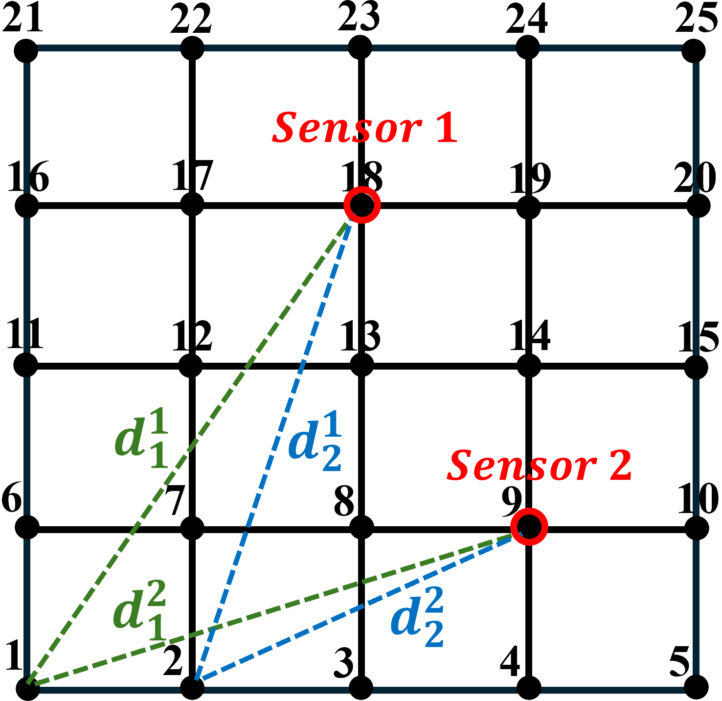
Figure 3: Illustration of sensor reconfiguration cost.

Proposition 2.

The modified CRMI $I^{\mathrm{mod}}(\boldsymbol{q})$ is submodular.

Proof.

See the Appendix. ∎

3.6 Convergence of the Proposed CSCP Algorithm

In this section, we show that the proposed CSCP algorithm converges in a finite number of iterations. To this end, first consider the following result.

Proposition 3.

If $A$ is Hurwitz, then the CSCP algorithm terminates in a finite number of iterations.

Proof.

If all modes of $A$ are stable, then the pair $(A,C_{k}(\boldsymbol{q}))$ is uniformly detectable for any $\boldsymbol{q}.$ Furthermore, because $Q=\sigma_{P}^{2}\boldsymbol{I}_{N_{\mathrm{P}}},$ the pair $(A,Q)$ is controllable. By [43] it follows that the estimation error is exponentially stable. Consequently, for any $\varepsilon>0$ there is a finite iteration number $M\in{\rm Nature}$ such that $\mathrm{tr}(P_{k})\leqslant\varepsilon,$ after which the CSCP algorithm terminates. ∎

Remark 1.

Whereas Proposition 3 is sufficient, it is not necessary for the convergence of the CSCP algorithm. A less restrictive criterion for convergence, which does not assume $A$ to be Hurwitz, is discussed below.

At the $k^{\mathrm{th}}$ iteration of the CSCP method, the predicted error covariance is defined as $P_{k|k-1}:=AP_{k-1|k-1}A^{\intercal}+Q_{k-1}$. Here, the term $AP_{k-1|k-1}A^{\intercal}$ grows the uncertainty from the previous step’s posterior covariance based on the $A$, and $Q_{k-1}$ accounts for the uncertainty introduced due to process noise. The measurement update is defined as $P_{k|k}:=P_{k|k-1}-L_{k}C_{k}P_{k|k-1}$. The uncertainty growth in the system is $\{P_{k|k-1}-P_{k-1|k-1}=AP_{k-1|k-1}A^{\intercal}-P_{k-1|k-1}+Q_{k-1}\}$. Similarly, the reduction in the uncertainty of the system after the measurement update is $\{P_{k|k-1}-P_{k|k}=L_{k}C_{k}P_{k|k-1}\}$. The convergence of the CSCP method is guaranteed if the following criterion is satisfied for every time steps.

$$\operatorname{tr}(L_{k}C_{k}P_{k|k-1})\geqslant\operatorname{tr}(AP_{k-1|k-1}A^{\intercal}-P_{k-1|k-1}+Q_{k-1}).$$

Note that this criterion cannot be verified a priori as it depends on the estimation error convariances computed during the algorithm’s execution.

4 Results and Discussion

In this section, we first provide an illustrative example of the proposed CSCP-CRMI method. Second, we compare the proposed method against a decoupled method that finds optimal sensor placement using the standard (path-independent) MI; for brevity we call this decoupled method CSCP-SMI. Third, we study the effects of varying numbers of sensors, threat parameters, and grid points on the CSCP-CRMI method. Fourth, we perform comparative study between the CSCP-CRMI and greedy sensor placements, and observe the equivalency as well as differences between the two approaches. Finally, we conduct a comparative study between the CSCP method with and without the sensor reconfiguration cost. All simulations are performed within a square workspace $\mathcal{W}=[-1,1]\times[-1,1]$ using non-dimensional units.

4.1 Illustrative Example

4

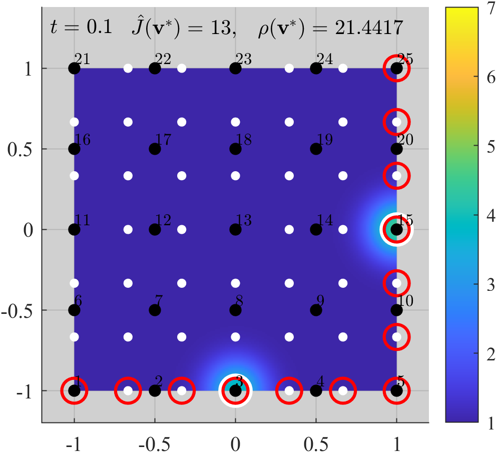
(a) $k=1$

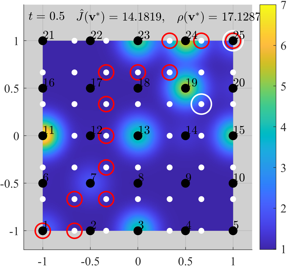
(b) $k=5$

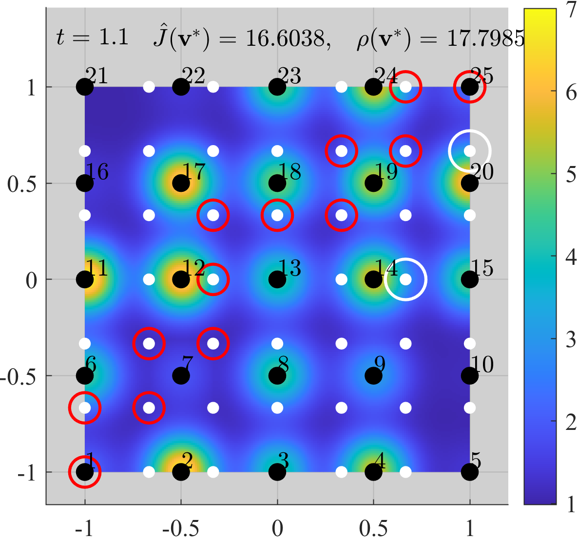
(c) $k=11$

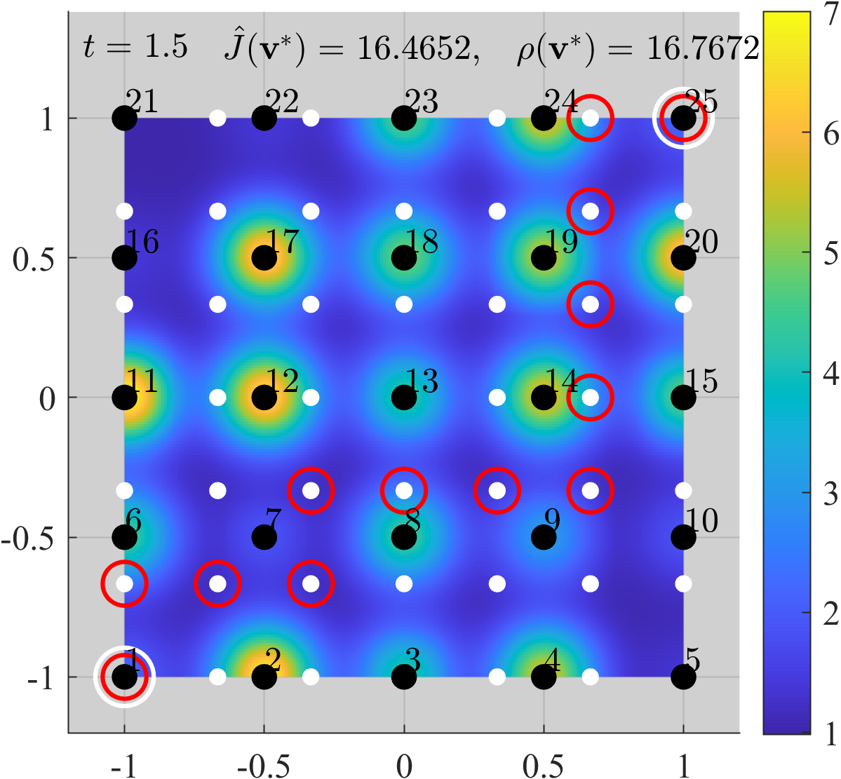
(d) $k=15$

Figure 4: Visualization of CSCP-CRMI process for $N_{\mathrm{P}}=25$ and $N_{\mathrm{G}}=49$.

2

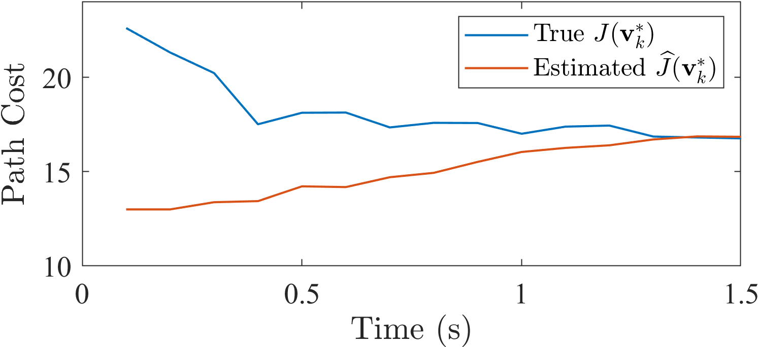
(a) Path cost mean.

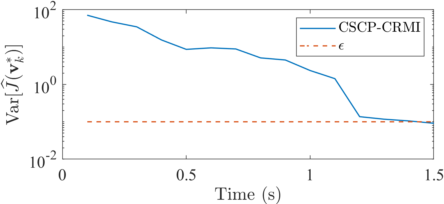
(b) Path cost variance.

Figure 5: Convergence of CSCP-CRMI algorithm.

The implementation of CSCP-CRMI algorithm on an illustrative example is shown in Fig. 4. The number of threat parameters, grid points, and sensors are $N_{\mathrm{P}}=25$, $N_{\mathrm{G}}=49$, and $N_{\mathrm{S}}=2$, respectively. The threat parameters $N_{\mathrm{P}}$, indicated by the black dots and numbered from 1 to 25, are uniformly spaced in the workspace. The white dots represent the grid points. The initial and the goal points are represented by the bottom left and the top right grid points in the map. The evolution of the threat field estimate $\widehat{c}$ for different time steps, namely $k=1,5,11$, and $15$ is shown by a colormap. The path $\boldsymbol{v}^{*}_{k}$ of minimum estimated cost is indicated by red circles, and the sensor placement $\boldsymbol{q}_{k}$ is shown by white circles, as illustrated in the Fig. 4(a)-(d). For a specified threshold $\varepsilon=0.1$, the algorithm terminates at $k=15$ iterations, and the optimal path $\boldsymbol{v}^{*}$ is achieved.

The comparison between the true and estimated path cost is illustrated in Fig. 5(a). Upon termination, the true and estimated path costs are nearly identical, with $J(\boldsymbol{v}^{*}_{k})=16.46$ and $\widehat{J}(\boldsymbol{v}^{*}_{k})=16.77$, respectively. Figure 5(b) shows the convergence of the proposed CSCP-CRMI algorithm. The path cost variance $\textrm{Var}[(\widehat{J}(\boldsymbol{v}^{*}_{k})]$ decreases with time, and the algorithm terminates in 15 iterations as the path cost variance decreases below 0.1.

2

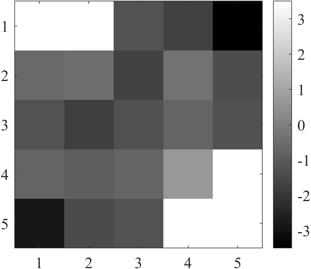
(a) CSCP-CRMI method

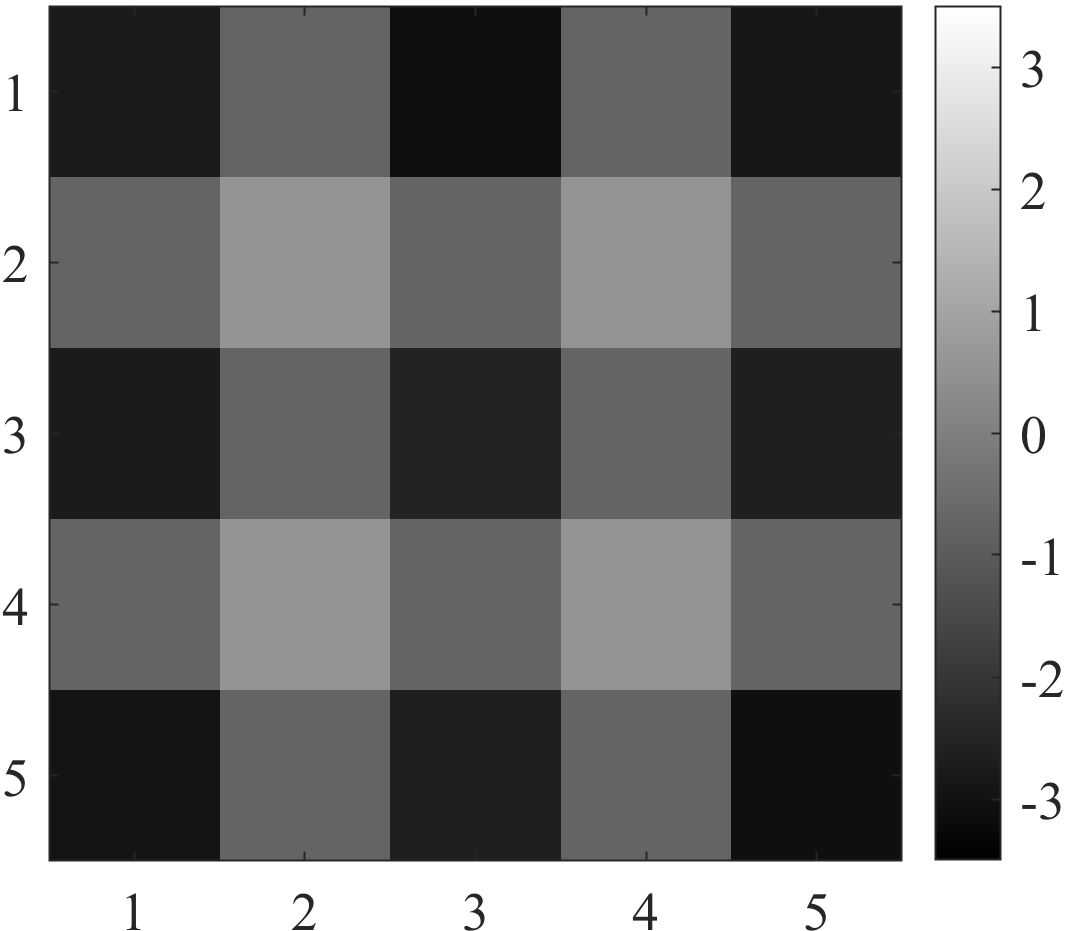
(b) CSCP-SMI method

Figure 6: Diagonal log-values of error covariance at final iteration.

4.2 Comparison of CSCP-CRMI and CSCP-SMI

For comparison, now consider the execution of CSCP-SMI on the same example as discussed above.

Figure 6 shows the estimation error covariance $P$ at the final iteration, mapped to the spatial regions of the environment using the centers of spatial basis functions $\Phi.$ In a slight departure from convention, Fig. 6 shows the logarithms of the diagonal values of $P,$ which explains the negative values despite $P$ being a symmetric positive definite matrix. The reason for this choice of logarithmic values is to clearly show the orders of magnitude difference in the estimation error covariance in different regions of the environment.

The white regions in Fig. 6 (a) with high error covariance represents the areas where few if any sensors are placed throughout the execution of CSCP-CRMI. The darker regions represent areas where sensors were placed to reduce the estimation error covariance values orders of magnitude below the white-colored regions. Compare Fig. 6 to the optimal path found in Fig. 4(d), and we find that the CSCP-CRMI sensor placement is such that areas close to the optimal path are those with low estimation error covariance. Note, crucially, the novelty of this approach: the optimal path is at first unknown, and that the sensor placement and path-planning are performed iteratively to arrive at these results.

2

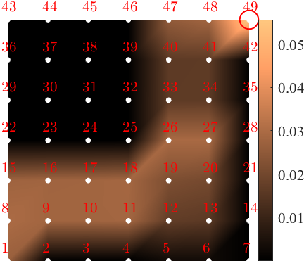
(a) CSCP-CRMI method

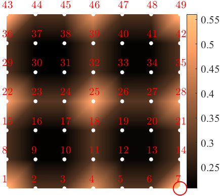
(b) CSCP-SMI method

Figure 7: Mutual information intensity map.

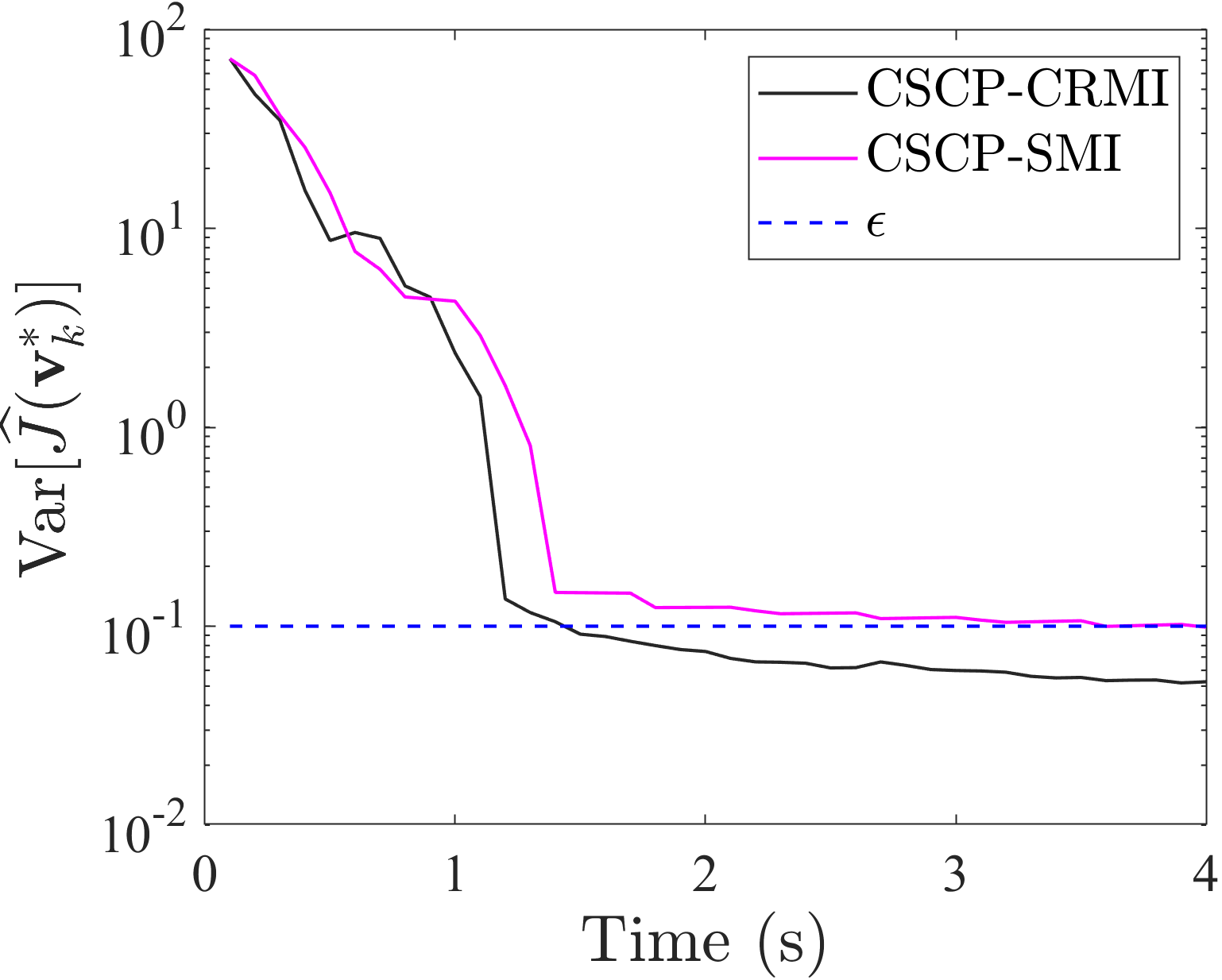
Figure 8: Comparison of path cost variance between CSCP-CRMI and CSCP-SMI with $N_{\mathrm{S}}=2$.

Figure 6 (b) shows the estimation error covariance $P$ of CSCP-SMI method. By contrast to Fig. 6 (a) for CSCP-CRMI, we note here spatially uniform covariance values. This means that in CSCP-SMI, the sensors are placed in such a way that the error covariances in all regions of the environment are low compared to CSCP-CRMI. Whereas this would be of benefit if we were merely trying to map the threat in the environment, this uniformly low error covariance is indicative of wasteful sensor placement in the context of path-planning. In case of CSCP-CRMI, although there are some regions in that are not explored, the outcome of the path-planning algorithm is still near-optimal.

An intensity map showing the mutual information values for each grid points from an illustrative example is shown in Fig. 7. Notably, these values are derived with consideration for only a single sensor. The brown regions represent the areas with higher CRMI values. It can be observed in Fig. 7 (a) that the CRMI regions are more visible around the vicinity of the path obtained in Fig. 4(d). Sensor is placed at the grid point, here number 49, with a maximum CRMI value. Similarly, Fig. 7(b) shows the SMI map representing the mutual information values between the state and measurement variables. The higher CRMI regions are observed around the location of the threat parameter, and for this example, sensor is placed at 7 numbered grid point.

2

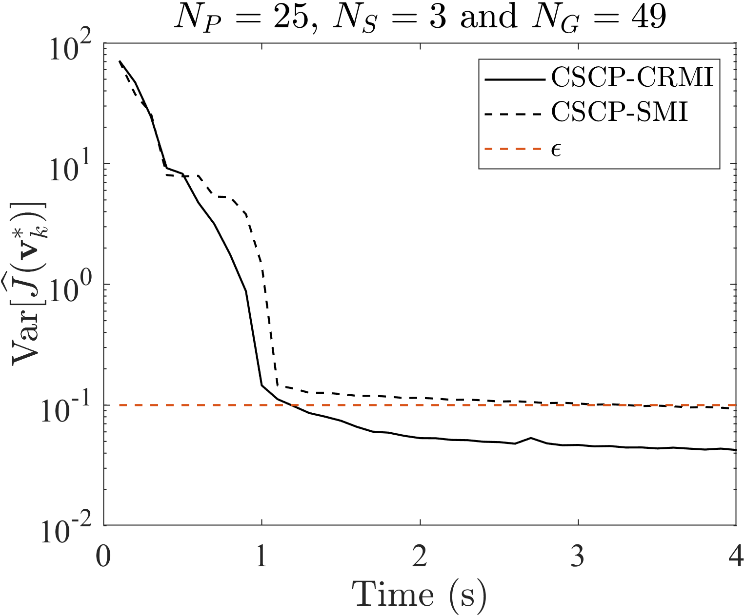
(a) $N_{\mathrm{S}}=3.$

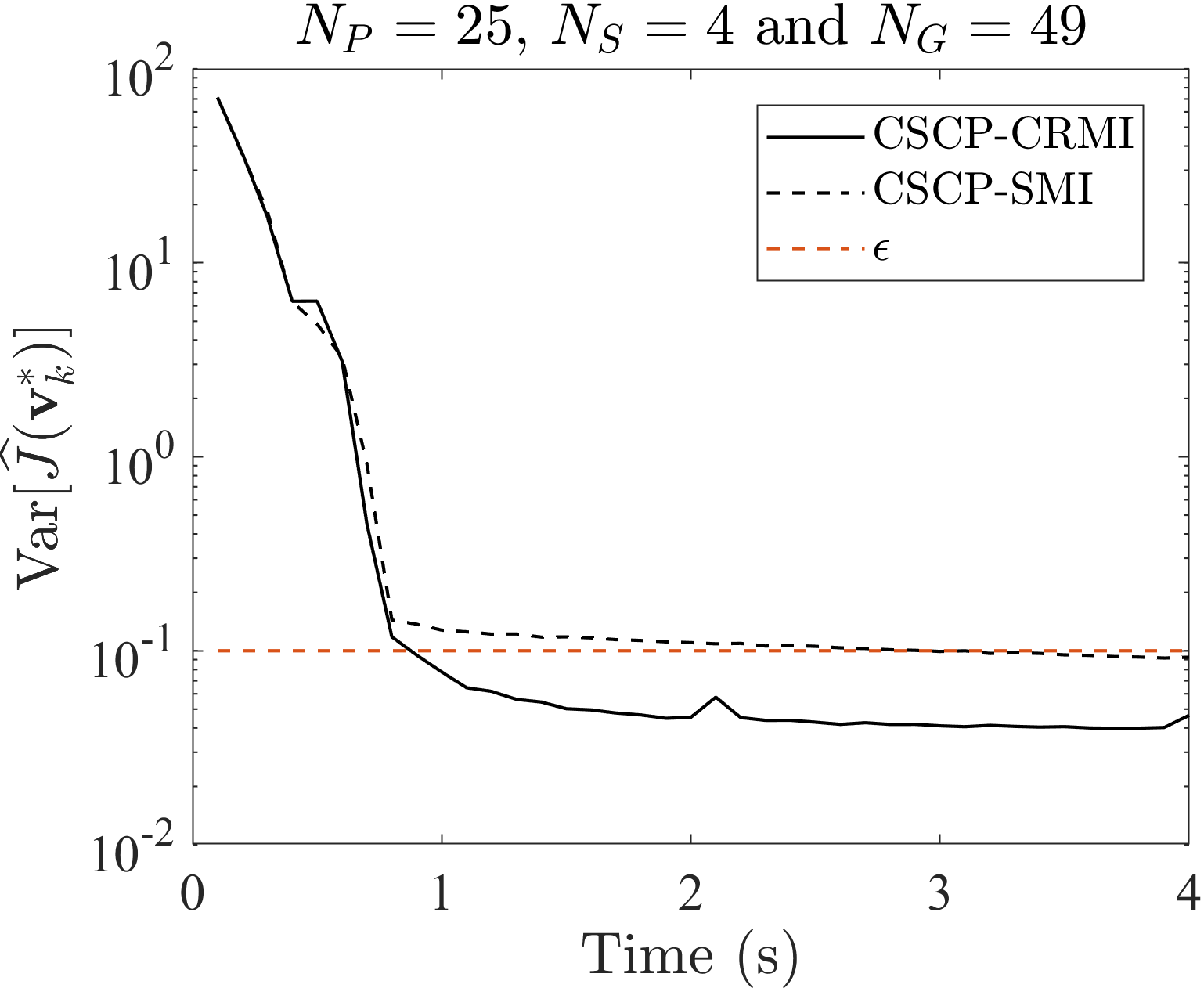
(b) $N_{\mathrm{S}}=4.$

Figure 9: Additional comparison of path cost variance between CSCP-CRMI and CSCP-SMI.

2

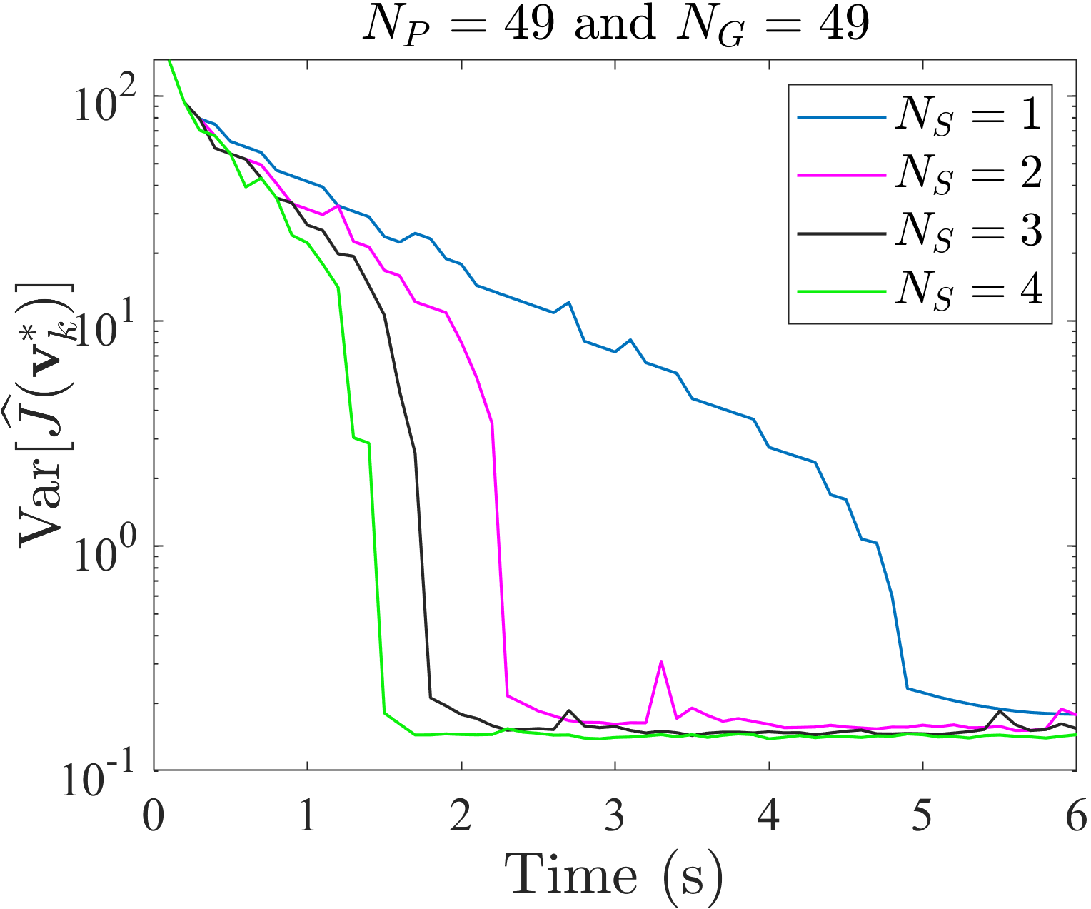
(a) Varying $N_{\mathrm{S}}$

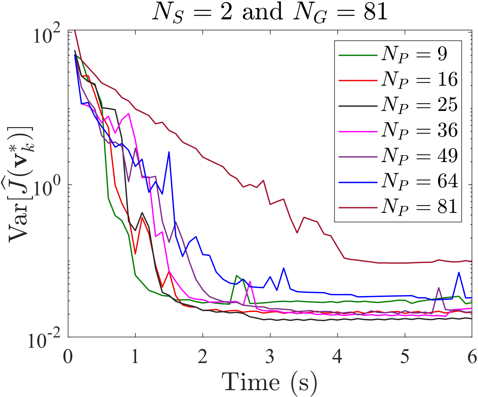
(b) Varying $N_{\mathrm{P}}$

Figure 10: Convergence of CSCP-CRMI algorithm for different number of sensors and parameters.

Figure 8 shows a comparison between the path cost variance $\textrm{Var}[{J}(\boldsymbol{v}^{*}_{k})]$ of the two methods. Note that for $\varepsilon=0.1$, the CSCP-SMI algorithm requires 39 iterations for convergence, which is 160% larger than the number of iterations required for CSCP-CRMI. Figure 9 shows similarly large differences in convergence rate for different numbers of sensors.

Figure 10(a) shows the variation of path cost variance with varying number of sensors. For a specified number of threat parameters $N_{\mathrm{P}}=49$ and the grid points $N_{\mathrm{G}}=49$, better convergence is achieved with more number of sensors. Using a single sensor will require a relatively large number of iterations for convergence.

The convergence of the CSCP-CRMI algorithm for different number of threat parameters $N_{\mathrm{P}}$ is shown in Fig. 10(b). For $N_{\mathrm{S}}=2$ and $N_{\mathrm{G}}=81$, CSCP converges faster for fewer threat states (e.g., $N_{\mathrm{P}}=9$ or $16$) compared to, say, $N_{\mathrm{P}}=64$ or $81$.

We also performed comparative analysis for specific number of sensors and parameters with varying number of grid points. It is observed that the path cost and the path cost variance remain unchanged for different number of grid points. This result is a consequence of proper scaling in the path cost formulation, namely, the scaling of the cost by the grid spacing $\delta.$

4.3 Analysis of Greedy Optimization

A comparative example of sensor placements for $N_{\mathrm{P}}=25,N_{\mathrm{G}}=25$, and $N_{\mathrm{S}}=4$ using greedy and non-greedy (true optimal) is shown in Fig. 11(a). Red circles in the figure indicate sensor positions with greedy placement, whereas the black circles indicate true optimal. Note that the two sensor locations in the grid space are common for both criteria. This is a specific example where greedy optimization results in the true optimal sensor configuration. In general, greedy optimization results in near-optimal configurations.

Figure 11(b) compares the time required to compute the optimal sensor configuration using the greedy and non-greedy approaches. The relative computing time is plotted for different combinations of grid points and number of sensors. As the number of sensors increases the relative computation time rapidly decreases, indicating the computational advantages of the greedy method. A sharp decrease on the relative computation time is observed especially as the number of grid points increases.

4

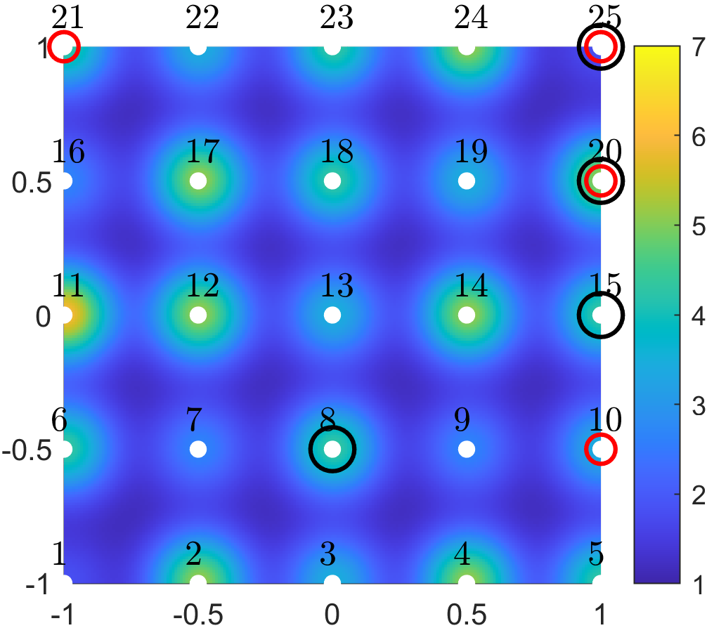
(a) Sensor locations.

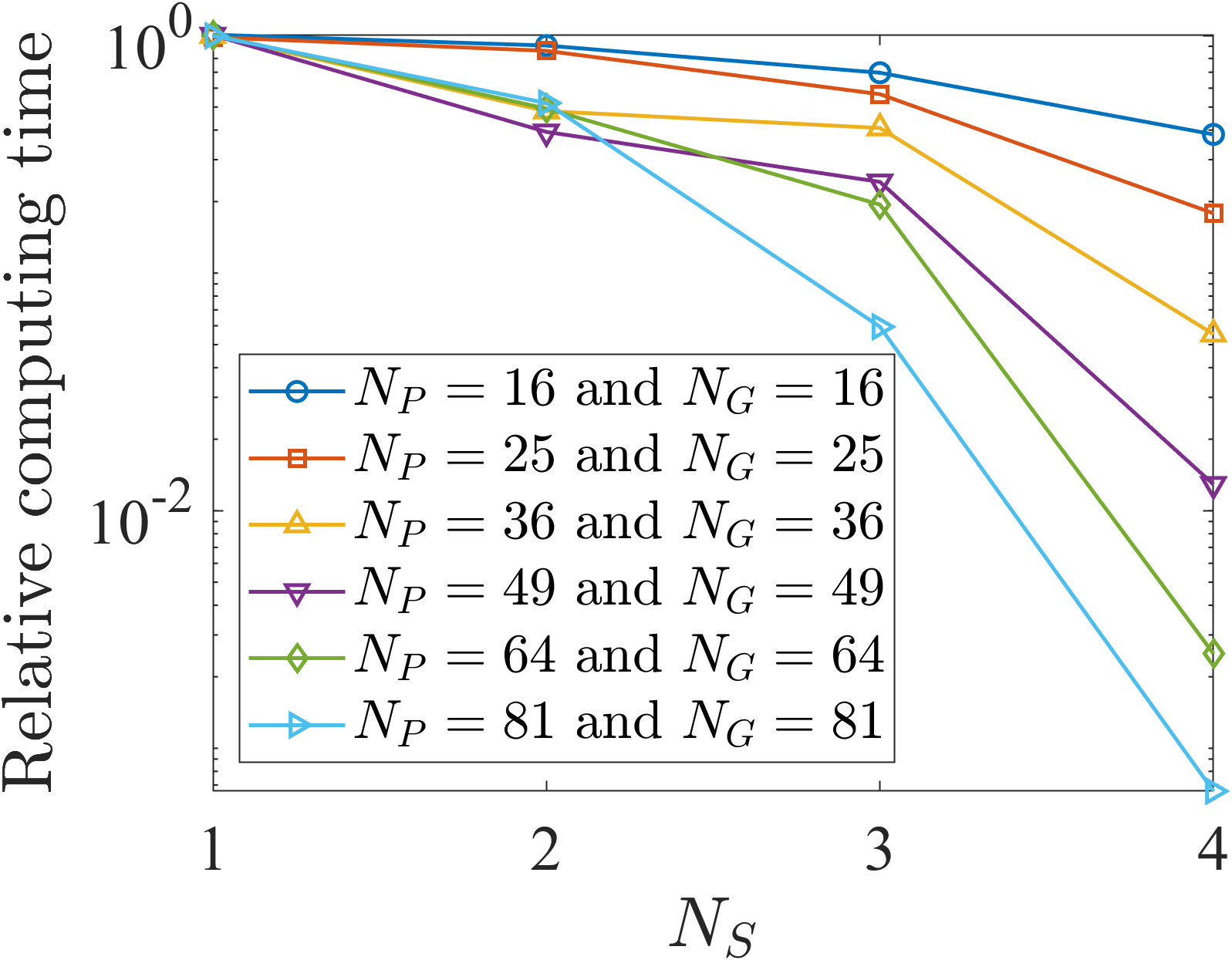
(b) Computation time.

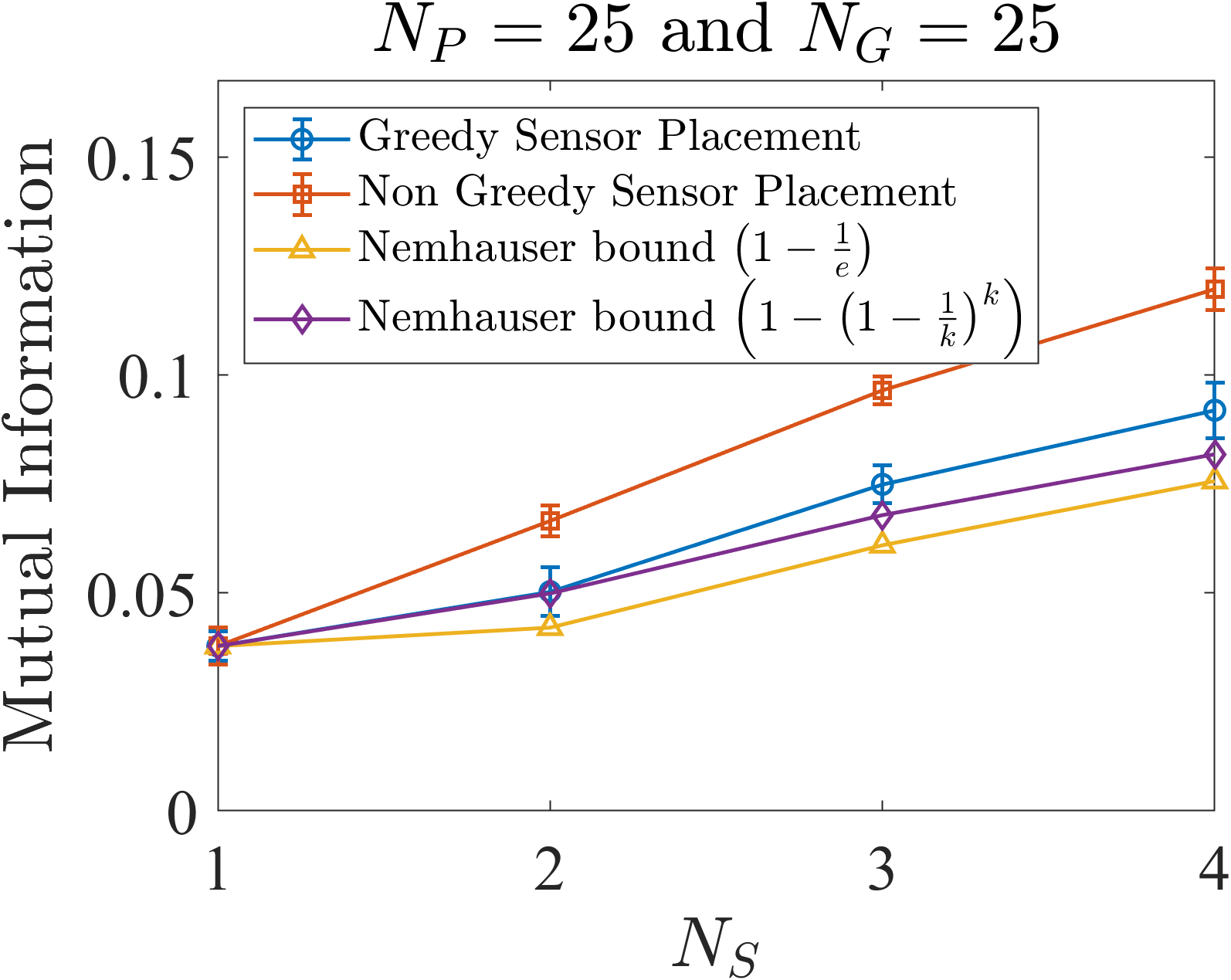
(c) Mutual information.

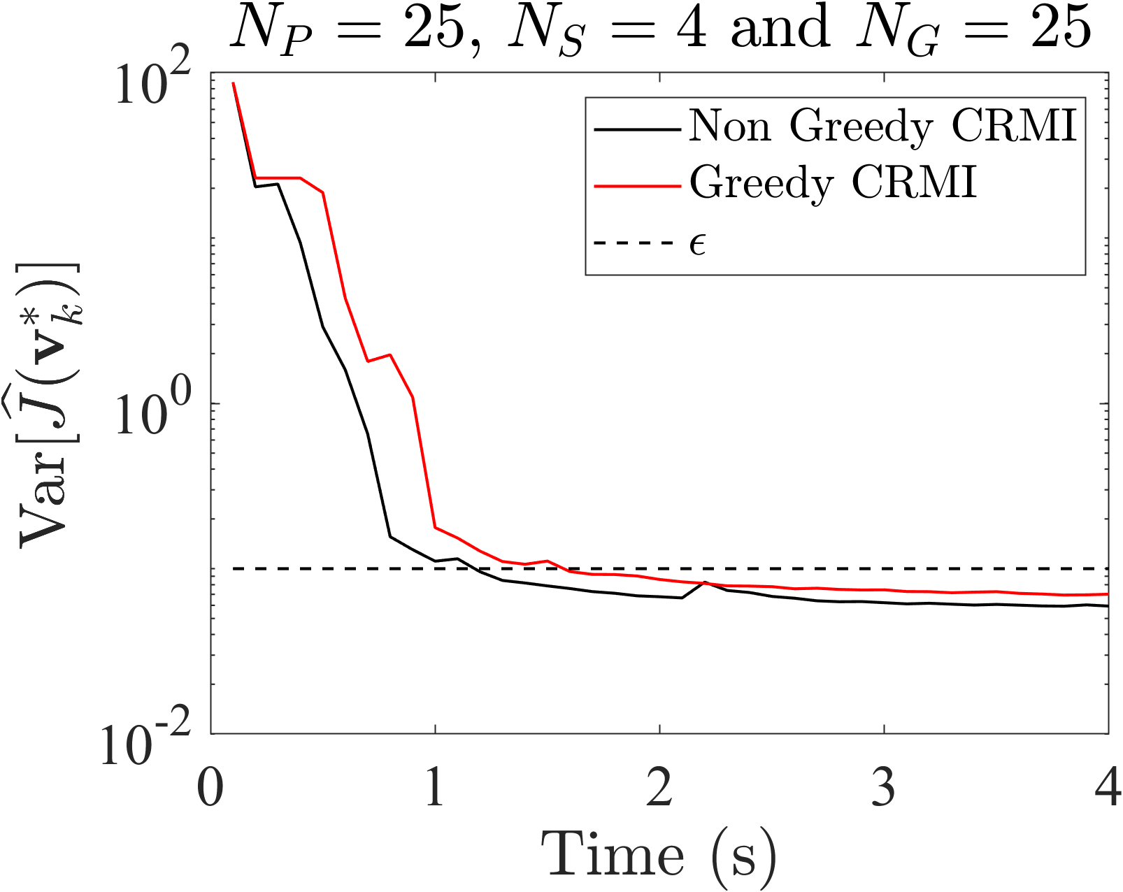
(d) Path cost variance.

Figure 11: Comparison between greedy and non greedy CSCP-CRMI process.

A comparison between the CRMI values for greedy and non-greedy methods is shown in Fig. 11(c). The suboptimality bounds described in Theorem 1 are also shown. As expected, Fig. 11(c) indicates that the greedy optimization-based CRMI values lie within these bounds. Finally, a comparison of the path cost variance is shown in Fig. 11(d). For this specific example and $\varepsilon=0.1$, the non-greedy (true optimal) method results in 12 CSCP iterations for convergence whereas the greedy method requires 16 CSCP iterations.

4.4 Analysis of Sensor Reconfiguration Cost

3

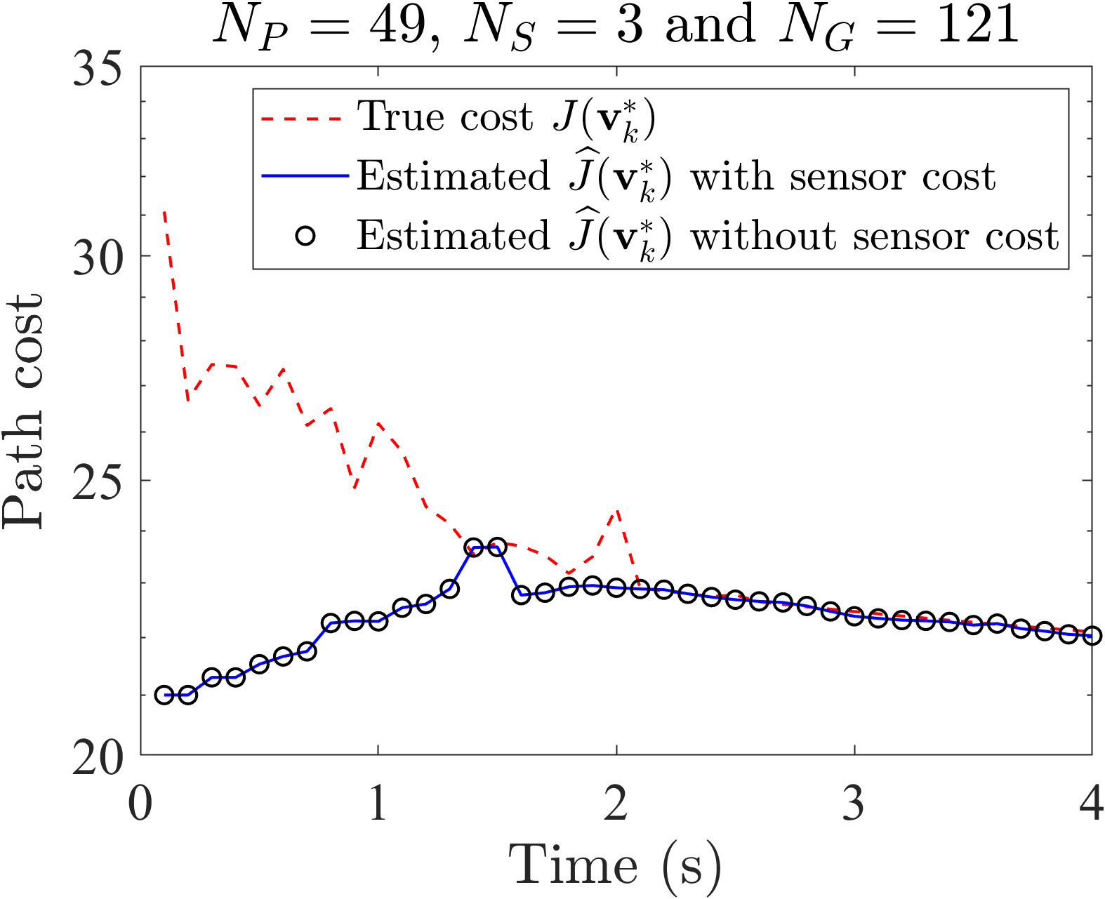
(a) Path cost mean.

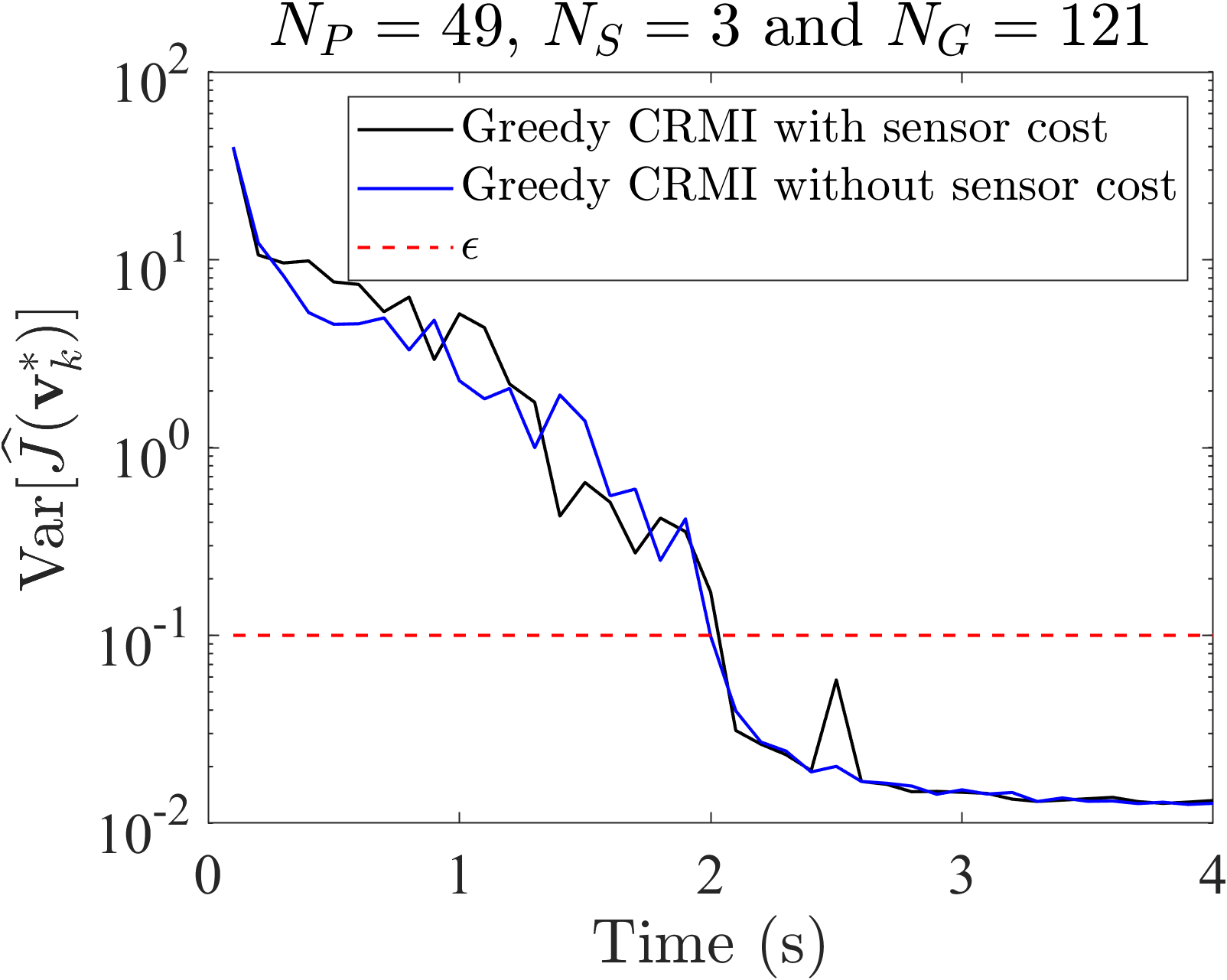
(b) Path cost variance.

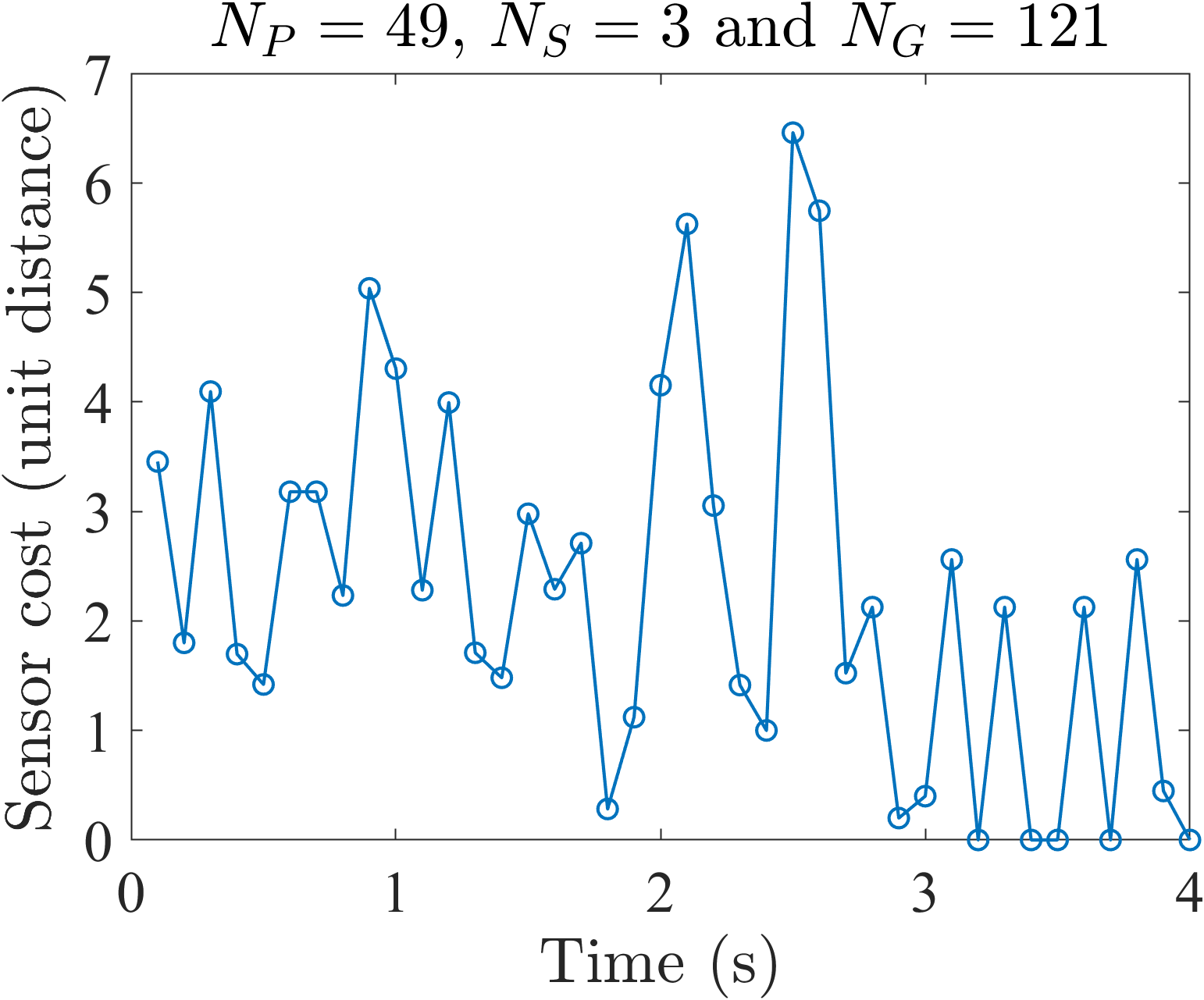
(c) Sum of distances traveled by sensors.

Figure 12: Path cost mean, variance over CSCP iterations with and without sensor reconfiguration cost.

The number of threat parameters, sensors, and the grid points used for the analysis are $N_{\mathrm{P}}=49$, $N_{\mathrm{S}}=3$, and $N_{\mathrm{G}}=121$, respectively. Figure 12(a) shows the comparison between the true and estimated mean path costs. Initially, the both estimated mean path costs are much lower than the true path cost. This is because there is not much information about the environment, and the estimator relies heavily on the “optimistic” prior, which results in threat estimates with small values. The estimated path costs for both with and without sensor reconfiguration costs are similar. The CSCP method with a sensor reconfiguration cost converges in 21 iterations, whereas the method without considering the sensor reconfiguration cost converges in 20 iterations. The convergence of both CSCP methods is shown by a path cost variance plot in Fig. 12(b). As the iterative process continues, the path cost variance $\textrm{Var}[(\widehat{J}(\boldsymbol{v}^{*}_{k})]$ decreases, and the algorithm terminates when $\textrm{Var}[(\widehat{J}(\boldsymbol{v}^{*}_{k})]$ falls below $\varepsilon=0.1$. Figure 12(c) shows the sensor reconfiguration cost values at different time steps. For the computation of sensor reconfiguration cost, we choose $\alpha_{1}=\sqrt{8}$ (diagonal distance across the workspace) and $\alpha_{2}=0.01.$ For $N_{\mathrm{S}}=3$, the sensor cost is the cumulative sum of the distance traveled by the three sensors at each iterations.

A comparative example of sensor placements for $N_{\mathrm{P}}=49,N_{\mathrm{G}}=121$, and $N_{\mathrm{S}}=4$ using CSCP with and without consideration of the sensor configuration cost is shown in Fig. 13(a) and (b). Red circles in the figure indicate sensor positions based on maximizing CRMI, whereas the black circles indicate sensor locations based on maximizing the modified CRMI. At $k=19$, it can be observed that the two sensor locations in the grid space are common for methods. As expected, when sensor reconfiguration cost is considered, the new sensor locations (black circles) at $k=20$ are relatively closer to the previous locations at $k=19$ as compared to sensor positions denoted by the red circles across the two iterations. Figure 13(c) shows the values of the CRMI and the modified CRMI for different numbers of sensors.

3

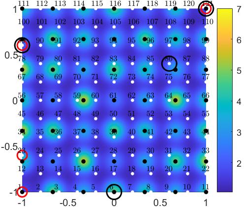
(a) Sensor locations at $k=19.$

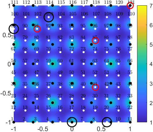
(b) Sensor locations at $k=20.$

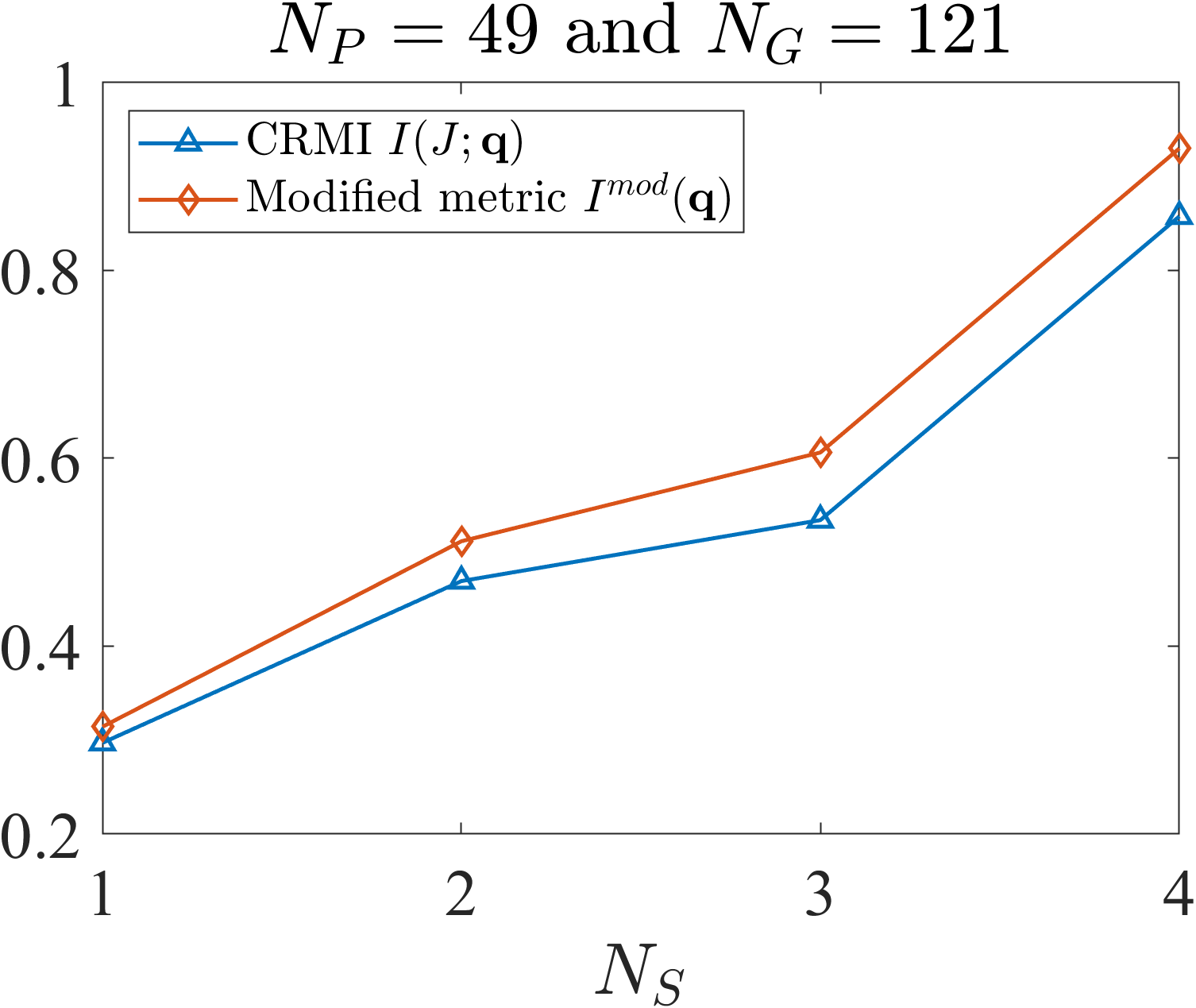
(c) CRMI and modified CRMI.

Figure 13: Comparison between the CSCP method with and without sensor reconfiguration cost.

4.5 Computational Complexity

The computational complexity of the Algorithm 1 depends on the complexity of CRMI optimization in Line 5, and the number of calls performed in Dijkstra’s algorithm in Line 9. CRMI calculation and maximization involves determinant and inverse computations, thus has a time complexity of $\mathcal{O}(N_{\mathrm{S}}^{3})$. By comparison, the CRMI calculation for the greedy optimization method has a complexity of $\mathcal{O}(N_{\mathrm{S}})$. The worst-case time complexity of Dijkstra’s algorithm implemented with a Fibonacci heap is $\mathcal{O}(N_{\mathrm{G}}+N_{\mathrm{G}}\log(N_{\mathrm{G}}))$ [34]. The complexity of CRMI optimization depends on the specific algorithm chosen.

5 Conclusions

In this paper, we discussed a new measure of information gain for optimal sensor placement to capture coupling of the sensor placement problem with a path-planning problem. This measure, which we call the context-relevant mutual information (CRMI), addresses the reduction in uncertainty in the path cost, rather than the environment state. We presented a coupled sensor placement and path-planning algorithm that iteratively places sensors based on CRMI maximization, updates the environment threat estimate, and then plans paths with minimum expected cost. Crucially, we showed CRMI to be a submodular function, due to which we can apply greedy optimization to arrive at near-optimal results while maintaining computational efficiency. We performed a comparative study between CSCP-CRMI and a decoupled CSCP-SMI method. The CSCP-SMI method places sensors by maximizing the standard (path-independent) mutual information of the measurments and threat state. We showed via numerical simulation examples that the CSCP-CRMI algorithm converges in less than half as many iterations compared to CSCP-SMI algorithm, which indicates a significant reduction in the number of sensor observations needed to find near-optimal paths. We also introduced and analyzed a modified cost function that addresses costs associated with distances traveled by sensors (i.e., sensor reconfiguration cost) after each iteration of placement.

Appendix

.1 Technical Proofs

Proof of Proposition 1.

By the definition of path relevant set $\mathcal{K}$, for the path $\boldsymbol{v}^{*}_{k}=\{v_{0},v_{1},\ldots,v_{L}\}$, the values of $\phi_{m}(\boldsymbol{x}_{\boldsymbol{v}_{\ell}})\approx 0$ for each $\ell=(0,1,\dots,L)$ and $m\notin\mathcal{K}$. Therefore, for all basis functions $m\notin\mathcal{K}$, $\boldsymbol{\Phi}(\boldsymbol{x}_{\boldsymbol{v}_{\ell}})=\boldsymbol{0}$, and by (10), $P_{{J\boldsymbol{z}}_{k|k-1}}\approx 0$. By (12), $I({J}_{k};\boldsymbol{z}_{k}(\boldsymbol{q}))\approx 0$ at locations in the workspace where the basis functions $\phi_{m}$ do not overlap with the path $\boldsymbol{v}$.

Per the proposed sensor reconfiguration policy, $\boldsymbol{q}^{*}_{k}=\max_{\boldsymbol{q}}I({J}_{k};\boldsymbol{z}_{k}(\boldsymbol{q}))$, sensors are necessarily placed at locations within the regions of significant support $\mathcal{R}_{m}^{\mathrm{sup}}$ defined by $\phi_{m}$, for each $m\in\mathcal{K},$ i.e., within the basis support regions of the basis functions contained within a path relevant set. Given the path cost $J(\boldsymbol{v})$ is known, the sensor measurements $\boldsymbol{z}(\boldsymbol{q})$ within the path-relevant set $\mathcal{K}$ fully capture the information about the $J(\boldsymbol{v})$. This shows that the sensor measurements are conditionally independent given the path cost. i.e., $p(\boldsymbol{z}_{1},\boldsymbol{z}_{2},\ldots\boldsymbol{z}_{N_{s}}\mid J)=p(z_{1}|J)p(z_{2}|J)\ldots p(\boldsymbol{z}_{N_{s}}\mid J).$ Next, we show that this conditional independence implies submodularity.

Consider two subsets of the sensor configurations, $\mathcal{A}$ and $\mathcal{B}$, such that $\mathcal{A}\subseteq\mathcal{B}\subseteq\boldsymbol{q}$, where $\boldsymbol{q}\subset\{N_{\mathrm{G}}\}.$ By (13), we write $I({J};\mathcal{A})=H(\mathcal{A})-H(\mathcal{A}\mid J)$ and $I({J};\mathcal{B})=H(\mathcal{B})-H(\mathcal{B}\mid J)$. For any $x\in\boldsymbol{q}\backslash\mathcal{B}$, the marginal CRMI gain due to a sensor placed at $x$ to in addition to those in sets $\mathcal{A}$ and $\mathcal{B}$ is

$$\Delta_{\mathcal{A}}(x) =I({J};\mathcal{A}\cup{x})-I({J};\mathcal{A}) =H(\mathcal{A}\cup{x})-H(\mathcal{A}\cup{x}\mid J)-H(\mathcal{A})+H(\mathcal{A}\mid J)$$

$$\Delta_{\mathcal{B}}(x) =I({J};\mathcal{B}\cup{x})-I({J};\mathcal{B}) =H(\mathcal{B}\cup{x})-H(\mathcal{B}\cup{x}\mid J)-H(\mathcal{B})+H(\mathcal{B}\mid J)$$

By the chain rule of conditional entropy, $H(\mathcal{A}\cup{x}\mid J)=H(\mathcal{A}\mid J)+H(x\mid\mathcal{A},J)$, and $H(\mathcal{B}\cup{x}\mid J)=H(\mathcal{B}\mid J)+H(x\mid\mathcal{B},J)$. Also, the conditional independence of $\boldsymbol{z}(\boldsymbol{q})$ given $J$ implies $H(x\mid\mathcal{A},J)=H(x\mid\mathcal{B},J)=H(x\mid J).$ It follows that

$$\Delta_{\mathcal{A}}(x) =H(\mathcal{A}\cup{x})-H(x\mid J)-H(\mathcal{A}), \Delta_{\mathcal{B}}(x) =H(\mathcal{B}\cup{x})-H(x\mid J)-H(\mathcal{B})$$

By the chain rule again, $H(\mathcal{A}\cup{x})=H(\mathcal{A})+H(x\mid\mathcal{A})$ and $H(\mathcal{B}\cup{x})=H(\mathcal{B})+H(x\mid\mathcal{B})$ from the previous expressions, we obtain $\Delta_{\mathcal{A}}(x)=H(x\mid\mathcal{A})-H(x\mid J)$, and $\Delta_{\mathcal{B}}(x)=H(x\mid\mathcal{B})-H(x\mid J)$. Therefore difference in marginal gains is $\Delta_{\mathcal{A}}(x)-\Delta_{\mathcal{B}}(x)=H(x\mid\mathcal{A})-H(x\mid\mathcal{B})$, which must be nonnegative because $\mathcal{A}\subseteq\mathcal{B}.$ Consequently, $I({J};\mathcal{A}\cup{x})-I({J};\mathcal{A})\geqslant I({J};\mathcal{B}\cup{x})-I({J};\mathcal{B})$, which satisfies the submodularity criterion. ∎

Proof of Proposition 2.

The sensor reconfiguration cost function can be represented as a set function

$$f(\mathcal{S}):=\alpha_{1}-\alpha_{2}\min_{j\in\{N_{\mathrm{S}}\},\ell\in\mathcal{S}}\left\{\|q_{\ell}-q_{j}^{k*}\|\right\},$$

where $\mathcal{S}\subseteq\{N_{\mathrm{S}}\}$ is a subset of sensor indices. Consider two subsets $\mathcal{A}$ and $\mathcal{B}$, such that $\mathcal{A}\subseteq\mathcal{B}\subseteq\{N_{\mathrm{S}}\}$ and $x\in\{N_{\mathrm{S}}\}\backslash\mathcal{B}$. In the rest of this proof, the symbol $j$ is an index over $\{N_{\mathrm{S}}\},$ i.e., $j\in\{N_{\mathrm{S}}\},$ which we avoid writing explicitly for notational convenience. Without loss of generality, we assume $\alpha_{2}=1.$

To calculate the marginal costs due to the inclusion of the index $x$ in either $\mathcal{A}$ or $\mathcal{B},$ we note:

$$f(\mathcal{A}\cup x) =\alpha_{1}-\min_{\ell\in\{\mathcal{A}\cup x\}}\|q_{\ell}-q_{j}^{k*}\|$$

$$f(\mathcal{B}\cup x) =\alpha_{1}-\min_{\ell\in\{\mathcal{B}\cup x\}}\|q_{\ell}-q_{j}^{k*}\|$$

$$\Rightarrow f(\mathcal{A}\cup x)-f(\mathcal{A}) =-\min_{\ell\in\{\mathcal{A}\cup x\}}\|q_{\ell}-q_{j}^{k*}\|+\min_{\ell\in\mathcal{A}}\|q_{\ell}-q_{j}^{k*}\|$$

$$\Rightarrow f(\mathcal{B}\cup x)-f(\mathcal{B}) =-\min_{\ell\in\{\mathcal{B}\cup x\}}\|q_{\ell}-q_{j}^{k*}\|+\min_{\ell\in\mathcal{B}}\|q_{\ell}-q_{j}^{k*}\|$$

Since $\mathcal{A}\subseteq\mathcal{B}$, $\min_{\ell\in\mathcal{A}}\|q_{\ell}-q_{j}^{k*}\|\geqslant\min_{\ell\in\mathcal{B}}\|q_{\ell}-q_{j}^{k*}\|.$ It follows that, for sufficiently large $\alpha_{1},$ $f(\mathcal{A})\leqslant f(\mathcal{B})$. Then we consider the following three cases:

$$\|q_{x}-q_{j}^{k*}\|\leqslant\min_{\ell\in\mathcal{B}}\|q_{\ell}-q_{j}^{k*}\|\leqslant\min_{\ell\in\mathcal{A}}\|q_{\ell}-q_{j}^{k*}\|,$$ (i)

$$\min_{\ell\in\mathcal{B}}\|q_{\ell}-q_{j}^{k*}\|\leqslant\|q_{x}-q_{j}^{k*}\|\leqslant\min_{\ell\in\mathcal{A}}\|q_{\ell}-q_{j}^{k*}\|,$$ (ii)

$$\min_{\ell\in\mathcal{B}}\|q_{\ell}-q_{j}^{k*}\|\leqslant\min_{\ell\in\mathcal{A}}\|q_{\ell}-q_{j}^{k*}\|\leqslant\|q_{x}-q_{j}^{k*}\|.$$ (iii)

For case (i) we note:

$$f(\mathcal{A}\cup x)-f(\mathcal{A}) =\min_{\ell\in\mathcal{A}}\|q_{\ell}-q_{j}^{k*}\|-\|q_{x}-q_{j}^{k*}\|,$$

$$f(\mathcal{B}\cup x)-f(\mathcal{B}) =\min_{\ell\in\mathcal{B}}\|q_{\ell}-q_{j}^{k*}\|-\|q_{x}-q_{j}^{k*}\|$$

It follows that $f(\mathcal{A}\cup x)-f(\mathcal{A})>f(\mathcal{B}\cup x)-f(\mathcal{B})$. For case (ii) we note:

$$f(\mathcal{A}\cup x)-f(\mathcal{A}) =\min_{\ell\in\mathcal{A}}\|q_{\ell}-q_{j}^{k*}\|-\|q_{x}-q_{j}^{k*}\|,$$

$$f(\mathcal{B}\cup x)-f(\mathcal{B}) =\min_{\ell\in\mathcal{B}}\|q_{\ell}-q_{j}^{k*}\|-\min_{\ell\in\mathcal{B}}\|q_{\ell}-q_{j}^{k*}\|=0.$$

Again, it follows that $f(\mathcal{A}\cup x)-f(\mathcal{A})>f(\mathcal{B}\cup x)-f(\mathcal{B})$. Finally, for case (iii) we note:

$$f(\mathcal{A}\cup x)-f(\mathcal{A})=f(\mathcal{B}\cup x)-f(\mathcal{B})=0.$$

Therefore, the inequality $f(\mathcal{A}\cup x)-f(\mathcal{A})\geqslant f(\mathcal{B}\cup x)-f(\mathcal{B})$ is always true and $f$ is submodular. By Proposition 1 and the additive property of submodular functions [42], $I^{\mathrm{mod}}(\boldsymbol{q})$ is submodular. ∎

.2 Unscented Kalman Filter for Threat Estimation

The estimated state parameters and the error covariance of the system are calculated by an Unscented Kalman Filter (UKF) [3]. Although the scope of this paper is limited to linear threat field dynamics, we would like to ensure generality for nonlinear threat models to be considered in the future. For the reader’s convenience we provide a brief overview of the UKF here and refer to [3] for further details.

An augmented state variable $\boldsymbol{\Theta}_{k-1}^{a}\in[N_{\boldsymbol{\Theta}}+N_{\boldsymbol{\omega}}+N_{\boldsymbol{\eta}}]$ is defined as $\boldsymbol{\Theta}_{k-1}^{a}=[\boldsymbol{\Theta}^{T}_{k-1}\quad\boldsymbol{\omega}^{T}_{k-1}\quad\boldsymbol{\eta}^{T}_{k-1}]^{T}$ and $2N+1$ sigma vectors are initialized using augmented estimated states $\widehat{\boldsymbol{\Theta}}_{k-1}^{a}$ and error covariance $P^{a}_{k-1}$ as:

$$\boldsymbol{\sigma}^{a}_{k-1} :=\left[\widehat{\boldsymbol{\Theta}}_{k-1}^{a}\cdots\widehat{\boldsymbol{\Theta}}_{k-1}^{a}\right]+\left[\textbf{0}\quad\sqrt{(N+\lambda)P^{a}_{k-1}}\quad-\sqrt{(N+\lambda)P^{a}_{k-1}}\right].$$

The generated sigma vectors are propagated through the process model as $\boldsymbol{\sigma}^{\boldsymbol{\Theta}}_{k|k-1}=\textbf{A}\boldsymbol{\sigma}^{\boldsymbol{\Theta}}_{k-1}+\boldsymbol{\sigma}^{\boldsymbol{\omega}}_{k-1}$, where $\boldsymbol{\sigma}^{\boldsymbol{\Theta}}_{k-1}$ and $\boldsymbol{\sigma}^{\boldsymbol{\omega}}_{k-1}$ are the components of $\boldsymbol{\sigma}^{a}$ that correspond to the state variables and process noise, respectively. At time instants where measurements are not available, the estimated state and error covariance are predicted as

$$\widehat{\boldsymbol{\Theta}}_{k}^{-} =\sum_{i}^{2N}W_{i}^{(m)}\sigma^{\boldsymbol{\Theta}}_{i,k|k-1},$$

$${P}_{k}^{-} =\sum_{i}^{2N}W_{i}^{(c)}\left(\boldsymbol{\sigma}^{\boldsymbol{\Theta}}_{i,k|k-1}-\widehat{\boldsymbol{\Theta}}_{k}^{-}\right){\left(\boldsymbol{\sigma}^{\boldsymbol{\Theta}}_{i,k|k-1}-\widehat{\boldsymbol{\Theta}}_{k}^{-}\right)}^{\intercal},$$

where, $W_{i}^{(m)}$ and $W_{i}^{(c)}$ are weights associated with sigma vectors. After the sensor measurements are taken, the measurement model is propagated using $\boldsymbol{\gamma}_{k|k-1}=C_{k}(\boldsymbol{q})\boldsymbol{\sigma}^{\boldsymbol{\Theta}}_{k|k-1}+\boldsymbol{\sigma}^{\boldsymbol{\eta}}_{k-1}$. Next, the mean and covariance of the measurement, and the cross-covariance of the state and measurement are calculated as:

$$\widehat{\boldsymbol{z}}_{k}^{-} =\sum_{i}^{2N}W_{i}^{(m)}\boldsymbol{\gamma}_{i,k|k-1},$$

$$P_{{\boldsymbol{z}\boldsymbol{z}}_{k}} =\sum_{i}^{2N}W_{i}^{(c)}\left(\boldsymbol{\gamma}_{i,k|k-1}-\widehat{\boldsymbol{z}}_{k}^{-}\right){\left(\boldsymbol{\gamma}_{i,k|k-1}-\widehat{\boldsymbol{z}}_{k}^{-}\right)}^{\intercal},$$

$$P_{{\boldsymbol{\Theta}\boldsymbol{z}}_{k}} =\sum_{i}^{2N}W_{i}^{(c)}\left(\boldsymbol{\sigma}^{\boldsymbol{\Theta}}_{i,k|k-1}-\widehat{\boldsymbol{\Theta}}_{k}^{-}\right){\left(\boldsymbol{\gamma}_{i,k|k-1}-\widehat{\boldsymbol{z}}_{k}^{-}\right)}^{\intercal}.$$

Finally, the filter gain is calculated as $L_{k}=P_{{\boldsymbol{\Theta}\boldsymbol{z}}_{k}}{P}^{-1}_{{\boldsymbol{z}\boldsymbol{z}}_{k}}$ and the estimated states, $\widehat{\boldsymbol{\Theta}}_{k}$ and covariance, $P_{k}$ are updated as, $\widehat{\boldsymbol{\Theta}}_{k}=\widehat{\boldsymbol{\Theta}}_{k}^{-}+L_{k}(\boldsymbol{z}_{k}-\widehat{\boldsymbol{z}}_{k}^{-})$, and $P_{k}=P_{k}^{-}-L_{k}P_{{\boldsymbol{z}\boldsymbol{z}}_{k}}L_{k}^{\intercal}$.

References

- Lewis et al. [2017] Lewis, F. L., Xie, L., and Popa, D., Optimal and robust estimation: with an introduction to stochastic control theory, CRC press, 2017.
- Thrun et al. [2006] Thrun, S., Burgard, W., and Fox, D., Probabilistic Robotics, The MIT Press, 2006.
- Julier and Uhlmann [2004] Julier, S., and Uhlmann, J., “Unscented filtering and nonlinear estimation,” Proceedings of the IEEE, Vol. 92, 2004, pp. 401–422. 10.1109/JPROC.2003.823141.
- Doucet and Johansen [2009] Doucet, A., and Johansen, A. M., “A tutorial on particle filtering and smoothing: Fifteen years later,” Handbook of nonlinear filtering, Vol. 12, No. 656-704, 2009, p. 3.
- LaValle [2006] LaValle, S. M., Planning Algorithms, Cambridge University Press, 2006.
- Patle et al. [2019] Patle, B., Pandey, A., Parhi, D., and Jagadeesh, A., “A review: On path planning strategies for navigation of mobile robot,” Defence Technology, Vol. 15, 2019, pp. 582–606. 10.1016/j.dt.2019.04.011.
- Popović et al. [2024] Popović, M., Ott, J., Rückin, J., and Kochenderfer, M. J., “Learning-based methods for adaptive informative path planning,” Robotics and Autonomous Systems, 2024, p. 104727.
- Chen et al. [2021] Chen, J., Du, C., Zhang, Y., Han, P., and Wei, W., “A clustering-based coverage path planning method for autonomous heterogeneous UAVs,” IEEE Transactions on Intelligent Transportation Systems, Vol. 23, No. 12, 2021, pp. 25546–25556.
- Chintam et al. [2024] Chintam, P., Lei, T., Osmanoglu, B., Wang, Y., and Luo, C., “Informed sampling space driven robot informative path planning,” Robotics and Autonomous Systems, Vol. 175, 2024, p. 104656.
- Rückin et al. [2022] Rückin, J., Jin, L., and Popović, M., “Adaptive Informative Path Planning Using Deep Reinforcement Learning for UAV-based Active Sensing,” International Conference on Robotics and Automation (ICRA), 2022, pp. 4473–4479. 10.1109/ICRA46639.2022.9812025.
- Qin et al. [2023] Qin, Y., Zhang, Z., Li, X., Huangfu, W., and Zhang, H., “Deep reinforcement learning based resource allocation and trajectory planning in integrated sensing and communications UAV network,” IEEE Transactions on Wireless Communications, Vol. 22, No. 11, 2023, pp. 8158–8169.
- Wen et al. [2024] Wen, T., Wang, X., Zheng, Z., and Sun, Z., “A DRL-based path planning method for wheeled mobile robots in unknown environments,” Computers and Electrical Engineering, Vol. 118, 2024, p. 109425.
- Kamil and Moghrabiah [2022] Kamil, F., and Moghrabiah, M. Y., “Multilayer decision-based fuzzy logic model to navigate mobile robot in unknown dynamic environments,” Fuzzy Information and Engineering, Vol. 14, No. 1, 2022, pp. 51–73.
- Ranieri et al. [2014] Ranieri, J., Chebira, A., and Vetterli, M., “Near-optimal sensor placement for linear inverse problems,” IEEE Transactions on Signal Processing, Vol. 62, 2014, pp. 1135–1146. 10.1109/TSP.2014.2299518.
- Kreucher et al. [2003] Kreucher, C., Kastella, K., and Hero III, A., “Information-based sensor management for multitarget tracking,” Proceedings of SPIE, Vol. 5204, 2003, pp. 480–489. 10.1117/12.502699.
- Soderlund and Kumar [2019] Soderlund, A. A., and Kumar, M., “Optimization of multitarget tracking within a sensor network via information-guided clustering,” Journal of Guidance, Control, and Dynamics, Vol. 42, 2019, pp. 317–334. 10.2514/1.G003656.
- Kasper et al. [2015] Kasper, K., Mathelin, L., and Abou-Kandil, H., “A machine learning approach for constrained sensor placement,” American Control Conference (ACC), 2015, pp. 4479–4484. 10.1109/ACC.2015.7172034.
- Wang et al. [2020] Wang, Z., Li, H.-X., and Chen, C., “Reinforcement learning-based optimal sensor placement for spatiotemporal modeling,” IEEE Transactions on Cybernetics, Vol. 50, 2020, pp. 2861–2871. 10.1109/TCYB.2019.2901897.
- Kangsheng and Guangxi [2006] Kangsheng, T., and Guangxi, Z., “Sensor management based on fisher information gain,” Journal of Systems Engineering and Electronics, Vol. 17, 2006, pp. 531–534.
- Wang et al. [2004] Wang, H., Yao, K., Pottie, G., and Estrin, D., “Entropy-based Sensor Selection Heuristic for Target Localization,” 3rd Int. Symp. Information Processing in Sensor Networks, 2004, pp. 36–45. 10.1145/984622.984628.
- Blasch et al. [2010] Blasch, E. P., Maupin, P., and Jousselme, A.-L., “Sensor-based allocation for path planning and area coverage using UGSs,” Proceedings of the IEEE 2010 National Aerospace & Electronics Conference, 2010, pp. 361–368. 10.1109/NAECON.2010.5712978.
- Krause et al. [2008] Krause, A., Singh, A., and Guestrin, C., “Near-optimal sensor placements in Gaussian processes: Theory, efficient algorithms and empirical studies.” Journal of Machine Learning Research, Vol. 9, No. 2, 2008.
- Robbiano et al. [2021] Robbiano, C., Azimi-Sadjadi, M. R., and Chong, E. K., “Information-Theoretic Interactive Sensing and Inference for Autonomous Systems,” IEEE Transactions on Signal Processing, Vol. 69, 2021, pp. 5627–5637.
- Hoffmann et al. [2020] Hoffmann, F., Charlish, A., Ritchie, M., and Griffiths, H., “Sensor Path Planning Using Reinforcement Learning,” IEEE 23rd International Conference on Information Fusion (FUSION), 2020, pp. 1–8. 10.23919/FUSION45008.2020.9190242.
- Jang et al. [2020] Jang, D., Yoo, J., Son, C. Y., Kim, D., and Kim, H. J., “Multi-robot active sensing and environmental model learning with distributed Gaussian process,” IEEE Robotics and Automation Letters, Vol. 5, No. 4, 2020, pp. 5905–5912.
- Park and Oh [2020] Park, M., and Oh, H., “Cooperative information-driven source search and estimation for multiple agents,” Information Fusion, Vol. 54, 2020, pp. 72–84.
- La et al. [2014] La, H. M., Sheng, W., and Chen, J., “Cooperative and active sensing in mobile sensor networks for scalar field mapping,” IEEE Transactions on Systems, Man, and Cybernetics: Systems, Vol. 45, No. 1, 2014, pp. 1–12.
- MacDonald and Smith [2019] MacDonald, R. A., and Smith, S. L., “Active sensing for motion planning in uncertain environments via mutual information policies,” The International Journal of Robotics Research, Vol. 38, No. 2-3, 2019, pp. 146–161.
- Li et al. [2021] Li, T., Wang, C., Meng, M. Q.-H., and de Silva, C. W., “Attention-driven active sensing with hybrid neural network for environmental field mapping,” IEEE Transactions on Automation Science and Engineering, Vol. 19, No. 3, 2021, pp. 2135–2152.
- Wu et al. [2020] Wu, K., Wang, H., Esfahani, M. A., and Yuan, S., “Achieving real-time path planning in unknown environments through deep neural networks,” IEEE Transactions on Intelligent Transportation Systems, Vol. 23, No. 3, 2020, pp. 2093–2102.
- Leong et al. [2014] Leong, A. S., Quevedo, D. E., Ahlén, A., and Johansson, K. H., “Network topology reconfiguration for state estimation over sensor networks with correlated packet drops,” IFAC Proceedings Volumes, Vol. 47, No. 3, 2014, pp. 5532–5537.
- Ramachandran et al. [2015] Ramachandran, G. S., Daniels, W., Matthys, N., Huygens, C., Michiels, S., Joosen, W., Meneghello, J., Lee, K., Canete, E., Rodriguez, M. D., et al., “Measuring and modeling the energy cost of reconfiguration in sensor networks,” IEEE Sensors Journal, Vol. 15, No. 6, 2015, pp. 3381–3389.
- Grichi et al. [2017] Grichi, H., Mosbahi, O., Khalgui, M., and Li, Z., “New power-oriented methodology for dynamic resizing and mobility of reconfigurable wireless sensor networks,” IEEE Transactions on Systems, Man, and Cybernetics: Systems, Vol. 48, No. 7, 2017, pp. 1120–1130.
- Cooper and Cowlagi [2019] Cooper, B. S., and Cowlagi, R. V., “Interactive planning and sensing in unknown static environments with task-driven sensor placement,” Automatica, Vol. 105, 2019, pp. 391–398. 10.1016/j.automatica.2019.04.014.
- St. Laurent and Cowlagi [2023] St. Laurent, C., and Cowlagi, R. V., “Near-optimal task-driven sensor network configuration,” Automatica, Vol. 152, 2023. 10.1016/j.automatica.2023.110966.
- Fang et al. [2021] Fang, J., Zhang, H., and Cowlagi, R. V., “Interactive Route-Planning and Mobile Sensing with a Team of Robotic Vehicles in an Unknown Environment,” AIAA Scitech 2021 Forum, 2021, p. 0865.
- Poudel and Cowlagi [2024] Poudel, P., and Cowlagi, R. V., “Coupled Sensor Configuration and Planning in Unknown Dynamic Environments with Context-Relevant Mutual Information-based Sensor Placement,” 2024 American Control Conference (ACC), IEEE, 2024, pp. 306–311.
- Poudel and Cowlagi [2025] Poudel, P., and Cowlagi, R. V., “Reconfiguration Costs in Coupled Sensor Configuration and Path-Planning for Dynamic Environments,” AIAA SCITECH 2025 Forum, 2025, p. 2069.
- Rockafellar and Uryasev [2000] Rockafellar, R. T., and Uryasev, S., “Optimization of conditional value-at-risk,” Journal of risk, Vol. 2, 2000, pp. 21–42.
- Cover and Thomas [1991] Cover, T., and Thomas, J., Elements of Information Theory, Wiley-Interscience, 1991.
- Adurthi et al. [2020] Adurthi, N., Singla, P., and Majji, M., “Mutual information based sensor tasking with applications to space situational awareness,” Journal of Guidance, Control, and Dynamics, Vol. 43, 2020, pp. 767–789. 10.2514/1.G004399.
- Nemhauser et al. [1978] Nemhauser, G. L., Wolsey, L. A., and Fisher, M. L., “An analysis of approximations for maximizing submodular set functions,” Mathematical programming, Vol. 14, 1978, pp. 265–294.
- Anderson and Moore [1981] Anderson, B. D., and Moore, J. B., “Detectability and stabilizability of time-varying discrete-time linear systems,” SIAM Journal on Control and Optimization, Vol. 19, No. 1, 1981, pp. 20–32.