Designing Scheduling for Diffusion Models via Spectral Analysis

Abstract

Diffusion models (DMs) have emerged as powerful tools for modeling complex data distributions and generating realistic new samples. Over the years, advanced architectures and sampling methods have been developed to make these models practically usable. However, certain synthesis process decisions still rely on heuristics without a solid theoretical foundation.

In our work, we offer a novel analysis of the DM’s inference process, introducing a comprehensive frequency response perspective. Specifically, by relying on Gaussianity and shift-invariance assumptions, we present the inference process as a closed-form spectral transfer function, capturing how the generated signal evolves in response to the initial noise. We demonstrate how the proposed analysis can be leveraged for optimizing the noise schedule, ensuring the best alignment with the original dataset’s characteristics. Our results lead to scheduling curves that are dependent on the frequency content of the data, offering a theoretical justification for some of the heuristics taken by practitioners.

1 Introduction

Diffusion Models (DMs) have become powerful tools for generating high-quality and diverse signals, with applications such as image generation, audio and video synthesis, and more. Alongside their practical success and the ability to handle complex distributions, some aspects of the diffusion processes still rely on heuristics rooted in empirical experimentation. A key example is choosing an appropriate noise schedule for the inference phase. Developing theoretical foundations for these heuristics may provide valuable insights into the diffusion process itself, and enable greater adaptation to different setups. Our work aims to provide such a theoretical backbone, as outlined below.

Our starting point is the fact that, while the continuous-time description of DMs via SDE or ODE (Song et al., 2021b) may be mathematically sound and well-founded, their practice necessarily deviates from these theoretical foundations, introducing various errors (Chen et al., 2023; Pierret & Galerne, 2024). A major source of this error is discretization, which replaces the DMs’ SDE/ODE formulations by their discrete-time approximations. Another source of error is the approximation error, originating from the gap between the ideal denoiser and its neural network realization.

Significant efforts have been made in recent work to minimize these associated errors and adapt DMs for real-world applications. Advanced numerical schemes for ODE and SDE solvers (Song et al., 2021b; Jolicoeur-Martineau et al., 2021; Zhang & Chen, 2023; Liu et al., 2022; Lu et al., 2022; Zheng et al., 2023; Zhao et al., 2024) offer various algorithmic ways for better treating the discretization of differential equations. An important aspect in all these methods is the decision on the time point discretization, which directly affects the synthesis quality. Realizing their importance, researchers have recently shifted their focus from custom-tailored heuristics (Ho et al., 2020; Nichol & Dhariwal, 2021; Karras et al., 2022; Chen, 2023) to the development of optimized noise schedules (Sabour et al., 2024; Tong et al., 2024; Watson et al., 2022; Wang et al., 2023; Xia et al., 2024; Chen et al., 2024; Xue et al., 2024; Williams et al., 2024). More on these methods and their relation to this paper’s contributions is detailed in Section 5.

In this work, we analyze the inference (reverse) diffusion process in the frequency domain, presenting the generated output signal as the outcome of a linear transfer function operating on the iid Gaussian input noise. This analysis is enabled by assuming that the destination distribution to sample from is Gaussian as well, and further assuming that it’s covariance is a Circulant matrix, inducing a shift-invariance hypothesis. Our mathematical formulation focuses on one-dimensional signals of varying lengths; the proposed analysis considers the dynamics of both DDPM (Ho et al., 2020) and DDIM (Song et al., 2021a), and extends the study for both variance preserving (VP) and variance exploding (VE) numerical schemes (Song et al., 2021b).

Posing the derived explicit expressions of the transfer systems as functions of the noise scheduling parameters, we may optimize a noise schedule tailored to a given dataset, its resolution, and the specified number of sampling steps required. We demonstrate how effectively solving these optimization problems numerically yields a noise schedule that accounts for these data characteristics, discuss their impact on the resulting schedule and validate our approach by comparing it with existing works. Finally, we apply the found scheduling to real-world scenarios using publicly available datasets, such as MUSIC (Moura et al., 2020) and SC09 (Warden, 2018), and demonstrate the relation to heuristic choices in past work and their improvement.

In summary, our contributions are the following: (i) Assuming a Gaussian distributed dataset, we present a novel spectral perspective on the discrete diffusion reverse process and derive a closed-form expression for its frequency transfer function. (ii) We formulate an optimization problem to find an optimal noise schedule that aligns with the dataset’s characteristics. Our approach provides an effective solution without relying on bounds or constraints on the number of diffusion steps. (iii) We compare our approach to existing work, showing that handcrafted noise scheduling decisions and related phenomena in the diffusion processes are often well-predicted by our approach. (iv) Our spectral analysis examines various setups, including DDIM and DDPM procedures, VP and VE formulations, the selection of loss functions, and additional features such as expectancy drift.

2 Background

We introduce the notations and the framework of diffusion probabilistic models, which are designed to generate samples $\mathbf{x}\in\mathbb{R}^{d}$ from an underlying, unknown probability distribution $p(\mathbf{x})$. While the diffusion process can be described as a Stochastic Differential Equation (SDE) or Ordinary Differential Equation (ODE), these formulations do not have general analytical solutions and are instead discretized and solved using numerical methods (Song et al., 2021b). Accordingly, we turn to describe the discrete formulations – DDPM (Ho et al., 2020) and DDIM (Song et al., 2021a) – which stand as the basis for our work.

The diffusion process is a generative procedure constructed from two stochastic paths: a forward and a reverse trajectories in which data flows (Ho et al., 2020). Each process is defined as a fixed Markovian chain composed of $T$ latent variables. During the forward process, a signal instance is gradually contaminated with white additive Gaussian noise as follows:

$$\mathbf{x}_{t}=\sqrt{\alpha_{t}}\mathbf{x}_{t-1}+\sqrt{1-\alpha_{t}}\boldsymbol{\epsilon}_{t}~,$$ (1)

where $\alpha_{t}$ for $t\in[1,T]$ is referred to as the incremental noise schedule and $\boldsymbol{\epsilon}_{t}\sim\mathcal{N}(\mathbf{0},\mathbf{I})$. Under the assumption that $\alpha_{T}$ is close to zero, we get that the final latent variable becomes $x_{T}\sim\mathcal{N}(\mathbf{0},\mathbf{I})$. A consequence of the above equation is an alternative relation of the form

$$\mathbf{x}_{t}=\sqrt{\bar{\alpha}_{t}}\mathbf{x}_{0}+\sqrt{1-\bar{\alpha}_{t}}\boldsymbol{\epsilon}~~~~~\boldsymbol{\epsilon}\sim\mathcal{N}(\mathbf{0},\mathbf{I})~,$$ (2)

for $\bar{\alpha}_{t}=\prod_{i=1}^{t}\alpha_{i}$. Based on the above relationships, the reverse process aims to reconstruct $\mathbf{x}_{0}$ from the noise $\mathbf{x}_{T}$ by progressively denoising it. This can be written as

$$\mathbf{x}_{t-1}=\frac{1}{\sqrt{{\alpha}_{t}}}\left(\mathbf{x}_{t}-\frac{1-\alpha_{t}}{\sqrt{1-\bar{\alpha}_{t}}}\boldsymbol{\epsilon}_{\theta}(\mathbf{x}_{t},t)\right)+\sigma_{t}\mathbf{z}_{t}~,$$ (3)

where $\boldsymbol{\epsilon}_{\theta}$ is the estimator of $\boldsymbol{\epsilon}$ for a given $\mathbf{x}_{t}$ at time $t$ with a neural network parameterized by $\theta$. In the above expression, $\sigma_{t}=\sqrt{\frac{1-\bar{\alpha}_{t-1}}{1-\bar{\alpha}_{t}}(1-\alpha_{t})}$   and   $\mathbf{z}_{t}\sim\mathcal{N}(\mathbf{0},\mathbf{I})$.

Alongside this stochastic formulation, Song et al. (2021a) provides a deterministic framework for the diffusion process, which can be utilized to enable faster sampling. DDIM models the forward process as a non-Markovian one, while preserving the same marginal distribution as in (2). As a result, the reverse process can be expressed by

$$\mathbf{x}_{s-1}=\sqrt{\bar{\alpha}_{s-1}}\left(\frac{\mathbf{x}_{s}-\sqrt{1-\bar{\alpha}_{s}}\cdot\boldsymbol{\epsilon}_{\theta}(\mathbf{x}_{s},s)}{\sqrt{\bar{\alpha}_{s}}}\right)\\ +\sqrt{1-\bar{\alpha}_{s-1}}\cdot\boldsymbol{\epsilon}_{\theta}(\mathbf{x}_{s},s),$$ (4)

where $s\in\left[0,S\right]$. Throughout the rest of the paper we denote by $\bar{\boldsymbol{\alpha}}$ the set of noise schedule parameters, $\left\{{{\bar{\alpha}}_{t}}\right\}_{t=0}^{T}$ for DDPM and $\left\{{{\bar{\alpha}}_{s}}\right\}_{s=0}^{S}$ for DDIM.

3 Analysis of Diffusion Processes

We consider the reverse process as a system that takes as input a noisy signal $\mathbf{x}_{T}$ and outputs $\mathbf{x}_{0}$. In this section, we develop the transfer function, which characterizes the relationship between these inputs and outputs in the frequency domain. To do so, we assume that the output signals are vectors drawn from a Gaussian distribution,

$$\mathbf{x}_{0}\sim\mathcal{N}(\boldsymbol{\mu}_{0},\boldsymbol{\Sigma}_{0})~,$$ (5)

where $\boldsymbol{\mu}_{0}\in\mathbb{R}^{d}$ and $\boldsymbol{\Sigma}_{0}\in\mathbb{R}^{d\times d}$. A similar assumption was used in previous work (Pierret & Galerne, 2024; Sabour et al., 2024). While this model greatly simplifies the signal’s distribution, we will demonstrate that it allows us to design a noise scheduling mechanism for different objectives.

3.1 The Optimal Denoiser for a Gaussian Input

The following theorem states a well-known fact: under the above Gaussianity assumption, the Minimum Mean-Squared Error (MMSE) denoiser operating on $\mathbf{x}_{t}$ to recover $\mathbf{x}_{0}$ is linear. It is the Wiener Filter (Wiener, 1949) and can be expressed in a closed form.

Theorem 3.1.

Let $\mathbf{x}_{0}\sim\mathcal{N}(\boldsymbol{\mu}_{0},\boldsymbol{\Sigma}_{0})$ and let $\mathbf{x}_{t}$ be defined by (2). Then, the denoised signal obtained from the MMSE (and the MAP) denoiser is given by:

$$\mathbf{x}^{*}_{0} = \left(\bar{\alpha}_{t}\boldsymbol{\Sigma}_{0}+(1-\bar{\alpha}_{t})\mathbf{I}\right)^{-1}$$

$$\hskip 28.90755pt\left(\sqrt{\bar{\alpha}_{t}}\boldsymbol{\Sigma}_{0}\mathbf{x}_{t}+\left(1-\bar{\alpha}_{t}\right)\boldsymbol{\mu}_{0}\right).$$

A detailed proof is given in Appendix A. Here, we outline the main steps. The MAP estimator seeks to maximize the posterior probability:

$$\max_{\mathbf{x}_{0}}\,\log p(\mathbf{x}_{0}|\mathbf{x}_{t})=\min_{\mathbf{x}_{0}}\,-\log p(\mathbf{x}_{t}|\mathbf{x}_{0})-\log p(\mathbf{x}_{0}).$$

By substituting the explicit density functions $p(\mathbf{x}_{0})$ and $p(\mathbf{x}_{t}|\mathbf{x}_{0})$ according to (2) into the above, and differentiating with respect to $\mathbf{x}_{0}$ we obtain the desired result. Under the assumption of Gaussian distributions, applying the MAP estimator is equivalent to minimizing the MSE, as both yield the same solution.

3.2 The Reverse Process in the Time Domain

We now turn to analyze the discrete sampling procedures, as introduced by Ho et al. (2020) and Song et al. (2021a), and described in Section 2. We begin by focusing on the DDIM formulation presented in Song et al. (2021a), as it highlights the fundamental principles more clearly and facilitates the analysis of faster sampling techniques.

The following lemma describes the relationship between two adjacent time steps during the inference process.

Lemma 3.2.

Assume $\mathbf{x}_{0}\sim\mathcal{N}(\boldsymbol{\mu}_{0},\boldsymbol{\Sigma}_{0})$ and let $\bar{\boldsymbol{\alpha}}$ be the noise schedule parameters, we have

$$\mathbf{x}_{s-1}=\left(a_{s}\mathbf{I}+b_{s}\sqrt{\bar{\alpha}_{s}}\bar{\boldsymbol{\Sigma}}^{-1}_{0,s}\boldsymbol{\Sigma}_{0}\right)\mathbf{x}_{s}\\ +b_{s}(1-\bar{\alpha}_{s})\bar{\boldsymbol{\Sigma}}^{-1}_{0,s}\boldsymbol{\mu_{0}},$$ (7)

where $\bar{\boldsymbol{\Sigma}}_{0,s}=\bar{\alpha}_{s}{\boldsymbol{\Sigma}}_{0}+(1-\bar{\alpha}_{s})\mathbf{I}$, and the coefficients are

$$a_{s}=\frac{\sqrt{1-\bar{\alpha}_{s-1}}}{\sqrt{1-\bar{\alpha}_{s}}}~~,~~b_{s}=\sqrt{\bar{\alpha}_{s-1}}-\frac{\sqrt{{\bar{\alpha}}_{s}}\sqrt{1-\bar{\alpha}_{s-1}}}{\sqrt{1-\bar{\alpha}_{s}}}~.$$

The above is obtained by plugging the optimal denoiser into the DDIM reverse process in (4). The derivation is given in Appendix B. This lemma establishes an explicit connection between adjacent diffusion steps, incorporating the characteristics of the destination signal density function as expressed by $\boldsymbol{\mu}_{0}$ and $\boldsymbol{\Sigma}_{0}$, along with the chosen noise schedule parameters $\bar{\boldsymbol{\alpha}}$.

3.3 Migrating to the Spectral Domain

Analyzing the diffusion process in the time domain can be mathematically and computationally challenging, particularly in high-dimensional spaces $(d\gg 1)$. To address this, we invoke a circular shift-invariance assumption and leverage the Discrete Fourier Transform (DFT), simplifying the analysis and enabling the examination of the signal’s frequency components.

Consider a destination signal $\mathbf{x}_{0}$ drawn from a multivariate Gaussian distribution with a fixed mean and a circulant covariance matrix. The DFT of $\mathbf{x}_{0}$, denoted $\mathbf{x}_{0}^{\mathcal{F}}$, also follows a Gaussian distribution. Specifically, $\mathbf{x}_{0}^{\mathcal{F}}\sim\mathcal{N}(\boldsymbol{\mu}_{0}^{\mathcal{F}},\boldsymbol{\Lambda}_{0})$, where $\boldsymbol{\mu_{0}}^{\mathcal{F}}$ is the transformed mean vector, and $\boldsymbol{\Lambda}_{0}$ is a positive semi-definite diagonal matrix, containing the eigenvalues of $\boldsymbol{\Sigma}_{0}$, denoted $\{\lambda_{i}\}_{i=1}^{d}$. These correspond to the DFT coefficients of its first row (Davis, 1970).

We now turn to describe the diffusion reverse process in the spectral domain. By applying the DFT to both sides of (7), we obtain the following result.

Lemma 3.3.

Assume $\mathbf{x}_{0}\sim\mathcal{N}(\boldsymbol{\mu}_{0},\boldsymbol{\Sigma}_{0})$ where $\boldsymbol{\Sigma}_{0}$ is a circulant matrix and let $\bar{\boldsymbol{\alpha}}$ be the noise schedule parameters. The subsequent step in the reverse process can be expressed in the frequency domain via

$$\mathbf{x}_{s-1}^{\mathcal{F}}=\mathbf{G}(s)\mathbf{x}_{s}^{\mathcal{F}}+\mathbf{M}(s)\boldsymbol{\mu_{0}}^{\mathcal{F}},$$ (8)

where $\mathbf{x}_{s}^{\mathcal{F}}$ denotes the DFT of the signal $\mathbf{x}_{s}$,

$$\mathbf{G}(s)=\left[a_{s}+b_{s}\sqrt{\bar{\alpha}_{s}}\left[\bar{\alpha}_{s}\mathbf{\Lambda}_{0}+(1-\bar{\alpha}_{s})\mathbf{I}\right]^{-1}\mathbf{\Lambda}_{0}\right]$$ (9)

and

$$\mathbf{M}(s)=b_{s}(1-\bar{\alpha}_{s})\left[\bar{\alpha}_{s}\mathbf{\Lambda}_{0}+(1-\bar{\alpha}_{s})\mathbf{I}\right]^{-1}~.$$ (10)

The lemma is proven in Appendix C. Equation (8) describes the relationship between two consecutive steps in the reverse process. Note that both matrices, $\mathbf{G}(s)$ and $\mathbf{M}(s)$, are diagonal, and thus, the reverse process in the frequency domain turns into a system of $d$ independent scalar equations.

Based on the above relationship, we may derive an expression for the generated signal in the frequency domain, denoted as $\mathbf{\hat{x}}_{0}^{\mathcal{F}}$. The complete derivation of the following result can be found in Appendix C as well.

Theorem 3.4.

Assume $\mathbf{x}_{0}\sim\mathcal{N}(\boldsymbol{\mu}_{0},\boldsymbol{\Sigma}_{0})$ where $\boldsymbol{\Sigma}_{0}$ is a circulant matrix and let $\bar{\boldsymbol{\alpha}}$ be the noise schedule parameters. The generated signal in the frequency domain $\hat{\mathbf{x}}_{0}^{\mathcal{F}}$ can be described as a function of $\mathbf{x}_{S}^{\mathcal{F}}$ via

$$\mathbf{\hat{x}}_{0}^{\mathcal{F}}=\mathbf{D}_{1}\mathbf{x}_{S}^{\mathcal{F}}+\mathbf{D}_{2}\boldsymbol{\mu_{0}}^{\mathcal{F}},$$ (11)

where $\mathbf{x}_{S}^{\mathcal{F}}\sim\mathcal{N}(\boldsymbol{0},\mathbf{I})$    and

$$\mathbf{D}_{1}=\prod_{k=1}^{S}\mathbf{G}(k)\quad\text{ , }\quad\mathbf{D}_{2}=\sum_{i=1}^{S}\left(\prod_{j=1}^{i-1}\mathbf{G}(j)\right)\mathbf{M}(i)~.$$

Moreover, $\mathbf{\hat{x}}_{0}^{\mathcal{F}}$ follows Gaussian distribution:

$$\mathbf{\hat{x}}_{0}^{\mathcal{F}}\sim\mathcal{N}(\mathbf{D}_{2}\boldsymbol{\mu_{0}}^{\mathcal{F}},\mathbf{D}_{1}^{2}),\quad\mathbf{\hat{x}}_{0}^{\mathcal{F}}\in\mathbb{R}^{d}.$$ (12)

Equation (11) provides a novel view of the generated signal in the frequency domain. Specifically, we can view (11) as a transfer function that models the relationship between the input signal $\mathbf{x}_{S}^{\mathcal{F}}$ and the output one, $\mathbf{\hat{x}}_{0}^{\mathcal{F}}$. Furthermore, since the matrices $\mathbf{D}_{1}$ and $\mathbf{D}_{2}$ are diagonal, the expression simplifies to a set of $d$ scalar transfer functions, with the only parameters being the noise schedule, $\bar{\boldsymbol{\alpha}}$.

So far, we examined DDIM. Similarly, a closed-form expression for the stochastic DDPM method (Ho et al., 2020) is presented in the following Theorem and is proven in Appendix E.

Theorem 3.5.

Assume $\mathbf{x}_{0}\sim\mathcal{N}(\boldsymbol{\mu}_{0},\boldsymbol{\Sigma}_{0})$ where $\boldsymbol{\Sigma}_{0}$ is a circulant matrix and let $\bar{\boldsymbol{\alpha}}$ be the noise schedule parameters. The signal $\hat{\mathbf{x}}_{0}^{\mathcal{F}}$ generated by DDPM can be expressed as a function of $\mathbf{x}_{T}^{\mathcal{F}}$ via

$$\mathbf{\hat{x}}_{0}^{\mathcal{F}}=\mathbf{D}_{1}\mathbf{x}_{T}^{\mathcal{F}}+\sum_{i=1}^{T}\left(\prod_{j=1}^{i-1}\mathbf{G}(j)\right)c_{i}\mathbf{z}^{\mathcal{F}}_{i}+\mathbf{D}_{2}\boldsymbol{\mu_{0}}^{\mathcal{F}}$$ (13)

where  $\mathbf{x}_{T}^{\mathcal{F}}\sim\mathcal{N}(\boldsymbol{0},\mathbf{I})$, $c_{i}=\sqrt{\frac{1-\bar{\alpha}_{i-1}}{1-\bar{\alpha}_{i}}(1-\alpha_{i})}~~$. The terms $\mathbf{D}_{1},\mathbf{D}_{2}$ and the matrices $\mathbf{G}(j)$ are defined in Appendix E. Moreover, $\mathbf{\hat{x}}_{0}^{\mathcal{F}}$ follows a Gaussian distribution:

$$\mathbf{\hat{x}}_{0}^{\mathcal{F}}\sim\mathcal{N}\!\!\left(\mathbf{D}_{2}\boldsymbol{\mu}_{0}^{\mathcal{F}}~,~\mathbf{D}_{1}^{2}+\sum_{i=1}^{T}\Big{(}\prod_{j=1}^{i-1}\mathbf{G}^{2}(j)\Big{)}c^{2}_{i}\mathbf{I}\right).$$ (14)

4 Optimal Spectral Schedules

With the closed-form expressions in (11) and (13), we can now explore different aspects of the diffusion process and examine how subtle changes in its design affect the output distribution. More specifically, a key aspect in this design is the choice of the noise schedule. In the discussion that follows we demonstrate how the proposed scheme enables optimal scheduler design.

We start by focusing on the direct dependence between the generated distribution and the noise schedule coefficients, $\bar{\boldsymbol{\alpha}}$. We define the probability density function of the output of the diffusion process in the frequency domain as $p(\mathbf{\hat{x}_{0}^{\mathcal{F}}};\bar{\boldsymbol{\alpha}})$. Our objective is to bring this distribution to become as close as possible to the original distribution, $p(\mathbf{{x}_{0}^{\mathcal{F}}})$. Specifically, given a dataset with a circulant covariance matrix, $\boldsymbol{\Sigma}_{0}$, defined by the eigenvalues $\{\lambda_{i}\}_{i=1}^{d}$ and $S$ diffusion steps, our goal is to identify the coefficients $\bar{\boldsymbol{\alpha}}$ that minimize some distance $\mathcal{D}$ between these two distributions. This results in the following optimization problem with a set of specified constraints:

$$\bar{\boldsymbol{\alpha}}^{*}=\arg\min_{\bar{\boldsymbol{\alpha}}}\mathcal{D}\left(p(\mathbf{\hat{x}_{0}^{\mathcal{F}}};\bar{\boldsymbol{\alpha}}),p(\mathbf{{x}_{0}^{\mathcal{F}}})\right)\\ \text{subject to}~~~\bar{\alpha}_{0}=1-\varepsilon_{0},~~~\bar{\alpha}_{S}=\varepsilon_{S},\\ \bar{\alpha}_{s-1}\geq\bar{\alpha}_{s}~\text{for}~s=1,\ldots,S.$$ (15)

The equality constraints ensure compatibility between the training and the synthesis processes. This involves ending the diffusion process with white Gaussian noise and starting it with very low noise to capture fine details in the objective distribution accurately (Lin et al., 2024). The inequality constraints align with the core principles of diffusion models and their gradual denoising process (Ho et al., 2020).

The distance $\mathcal{D}$ between the probabilities can be chosen depending on the specific characteristics of the task. In this work, we consider the Wasserstein-2 and Kullback-Leibler divergence, but other distances can also be used. The theorems presented below are detailed in Appendix D.

The Wasserstein-2 distance (or Earth Mover’s Distance) measures the minimal cost of transporting mass to transform one probability distribution into another. In the case of measuring a distance between two Gaussians, this has a closed-form expression.

Theorem 4.1.

The Wasserstein-2 distance $\mathcal{D}_{W_{2}}$ between the distributions $P(\mathbf{\hat{x}_{0}^{\mathcal{F}}};\bar{\boldsymbol{\alpha}})$ and $P(\mathbf{{x}_{0})^{\mathcal{F}}}$ is given by:

$$\mathcal{D}_{W_{2}}^{2}\big{(}P(\mathbf{\hat{x}_{0}^{\mathcal{F}}};\bar{\boldsymbol{\alpha}}),P(\mathbf{{x}_{0}^{\mathcal{F}})}\big{)}=\sum_{i=1}^{d}\left(\sqrt{\lambda_{i}}-[\mathbf{D}_{1}]_{i}\right)^{2}\\ +\sum_{i=1}^{d}[\boldsymbol{\mu}_{0}^{\mathcal{F}}]^{2}_{i}\,\left([\mathbf{D}_{2}]_{i}-1\right)^{2},$$ (16)

where $\{{\lambda}_{i}\}_{i=1}^{d}$ denote the $d$ eigenvalues of $\boldsymbol{\Sigma}_{0}$.

The KL divergence $D_{\mathrm{KL}}(P\|Q)$ assesses how much a model probability distribution $Q$ differs from a reference probability distribution $P$. Note that this divergence is not symmetric. As with the Wasserstein-2 case, here as well we obtain a closed-form expression for the two Gaussians considered.

Theorem 4.2.

The Kullback-Leibler divergence between the generated distribution $P(\mathbf{\hat{x}_{0}^{\mathcal{F}}};\bar{\boldsymbol{\alpha}})$ and the true distribution $P(\mathbf{{x}_{0}^{\mathcal{F}})}$ is given by

$$D_{\mathrm{KL}}(P(\mathbf{{x}_{0}^{\mathcal{F}})}\|P(\mathbf{\hat{x}_{0}^{\mathcal{F}}};\bar{\boldsymbol{\alpha}}))=\sum_{i=1}^{d}\log{[\mathbf{D}_{1}]_{i}}-\frac{1}{2}\sum_{i=1}^{d}\log{{\lambda}_{i}}\ \\ -\frac{d}{2}+\frac{1}{2}\sum_{i=1}^{d}\frac{{\lambda}_{i}+([\mathbf{D}_{2}]_{i}-1)^{2}{(\boldsymbol{\mu_{0}}^{\mathcal{F}})}_{i}^{2}}{[\mathbf{D}_{1}]_{i}^{2}}.$$ (17)

For solving the resulting optimization problems, we have employed the Sequential Least SQuares Programming (SLSQP) method (Kraft, 1988), a well-suited method for minimization problems with boundary conditions and equality and inequality constraints.

Before turning into the empirical evaluation of the proposed optimization, and the implications of the obtained noise scheduling on the various schemes, we pause to describe related work in this field.

5 Related Work

Recent work has acknowledged the importance of the noise scheduling in diffusion models, and the need to shift the focus from custom-tailored heuristics (Ho et al., 2020; Nichol & Dhariwal, 2021; Karras et al., 2022; Chen, 2023) to the development of optimized alternatives. For instance, Sabour et al. (2024) introduced the KL-divergence Upper Bound (KLUB), which minimizes the mismatch between the continuous SDE and its linearized approximation over short intervals. Subsequently, Tong et al. (2024) trained a student ODE solver with learnable discretized time steps by minimizing the KL-divergence to mimic a teacher ODE solver. However, these approaches, along with others (Watson et al., 2022; Wang et al., 2023; Xia et al., 2024), aim to minimize the estimation error as well, which requires retraining a denoiser or entailing substantial computation time and resources when solving the optimization problem.

While pursuing the same goal of optimizing the noise schedule, the work reported in Chen et al. (2024); Xue et al. (2024); Williams et al. (2024) made notable strides in simplifying the induced optimization problem. Chen et al. (2024) identified trajectory regularities in ODE-based diffusion sampling and optimized a noise schedule using dynamic programming. Xue et al. (2024) introduced an upper bound for the truncation error and treated the data-dependent component as negligible during optimization. Williams et al. (2024) proposed a predictor-corrector update approach and minimized the Stein divergence to provide a noise schedule based on score functions. Alongside these approaches’ scalability, a direct relationship between the dataset’s characteristics and the resulting noise schedule remains vague.

Spectral analysis, a fundamental tool in signal processing, can provide a bridge between the design choices and properties of diffusion models and the dataset’s characteristics. For instance, Rissanen et al. (2023) introduced the coarse-to-fine phenomenon, where diffusion models generate frequencies that evolve from a coarse structure to finer details. (Biroli et al., 2024) linked the memorization phenomenon with the dataset size. crabbe2024time connected signal localization in the frequency domain to successful frequency distribution modeling. Additionally, Yang et al. (2023); Corvi et al. (2023) applied frequency analysis to facilitate compact denoiser training and uncover spectral fingerprints across different architectures.

Despite significant progress in both areas, to our knowledge, no method has yet connected spectral analysis with the design of the noise schedule. A closely related approach is proposed by Pierret & Galerne (2024), where, under the centered Gaussian assumption, a closed-form solution to the SDE equation was derived, and the Wasserstein error was examined for selected ODE and SDE solvers. However, Pierret & Galerne (2024) did not address the noise schedule or its optimization.

6 Experiments

We turn to empirically validate the schedules obtained by solving the optimization problem, referring to them as the spectral schedule or spectral recommendation. We present three main scenarios, gradually progressing from the strict assumptions to more realistic conditions.

6.1 Scenario 1: Synthetic Gaussian Distribution

In the first set of experiments, we assume a Gaussian data distribution, $\mathbf{x}_{0}\sim\mathcal{N}(\boldsymbol{\mu}_{0},\boldsymbol{\Sigma}_{0})$, where $\mathbf{x}_{0}\in\mathbb{R}^{d}$ and $\boldsymbol{\Sigma}_{0}$ is a circulant matrix. The covariance is chosen to satisfy $\boldsymbol{\Sigma}_{0}=A^{T}A$ where $A$ is a circulant matrix whose first row is $a=[-l,-l+1/(d-1),\ldots,l-1/(d-1),l]$. The mean vector, $\boldsymbol{\mu}_{0}$, is chosen to be a constant-value vector, following the stationarity assumption.

Finding the optimal noise-schedule scheme $\bar{\boldsymbol{\alpha}}^{*}$ depends on the target signal characteristics $\left\{\lambda_{i}\right\}_{i=1}^{d}$, the resolution $d$, and the number of diffusion steps applied $S$. Figure 1 shows the resulting noise schedules for $d=50$, $l=0.1$ and $\boldsymbol{\mu_{0}}=0.05\!\cdot\!\mathbf{1}_{d}$, obtained by minimizing the Wasserstein-2 distance for different diffusion steps $[10,28,38,60,90,112,250,334]$. Further examples involving different forms of $\boldsymbol{\Sigma}_{0}$ and $\boldsymbol{\mu}_{0}$, as well as the use of the KL divergence, are provided in Appendix H

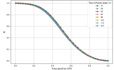
Figure 1: Optimized spectral schedules for Scenario 1 with $d=50$, $l=0.1$, and $\boldsymbol{\mu_{0}}=0.05\cdot\mathbf{1}_{d}$, obtained by minimizing the Wasserstein-2 distance for various numbers of diffusion steps.

At first glance, the optimization-based solution produces a noise schedule that aligns with the principles of diffusion models. Specifically, it exhibits a monotonically dicreasing behaviour, with linear drop in $\bar{\boldsymbol{\alpha}}^{*}$ in the middle of the process and minimal variation near the extremes. Although each schedule was independently optimized for a specified number of diffusion steps, it can be observed that the overall structure remains the same.

Interestingly, solving the optimization problem in (15) while altering the initial conditions or removing the inequality constraints yields the same optimal solution. This suggests that these constraints are passive, and that known characteristics of noise schedules, such as monotonicity, naturally arise from the problem’s formulation, as demonstrated in Appendix G.2.

A key aspect is how the optimal spectral noise schedule aligns with the existing heuristics. Figure 2 provides a comparison with the Cosine (Nichol & Dhariwal, 2021), the Sigmoid (Jabri et al., 2023), the linear (Ho et al., 2020) and the EDM $(\rho=7)$ (Karras et al., 2022) schedules, along with a parametric approximation of the spectral recommendation. To achieve this, Cosine and Sigmoid functions were fitted to the optimal solution by minimizing the $l_{2}$ loss, identifying the closest match.

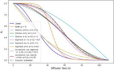
Figure 2: The spectral schedule (dotted gray) for $S=112$ diffusion steps is compared against various heuristic noise schedules. These include linear, EDM $(\rho=7)$ , and Cosine-based schedules such as Cosine ($s=0$,$e=1$,$\tau=1$) as in (Nichol & Dhariwal, 2021; Chen, 2023). Additionally, Sigmoid-based schedules like Sigmoid ($s=-3$,$e=3$,$\tau=1$) from (Jabri et al., 2023; Chen, 2023) are included. Parametric estimations for the Cosine and Sigmoid functions are shown in red and brown, respectively.

An interesting outcome from Figure 2 is that the spectral recommendation obtained provides a partial retrospective justification for existing noise schedule heuristics, as the parametric estimation resembles Cosine and Sigmoid functions, when their parameters are properly tuned.

To validate the optimization procedure, Figure 3 compares the Wasserstein-2 distance of various noise schedules with that of the spectral recommendation across different diffusion steps. While the spectral recommendation consistently achieves the lowest Wasserstein-2 distance, the optimization is most effective with fewer diffusion steps, where discretization errors are higher. As the number of steps increases, the gap between the different noise schedules narrows.

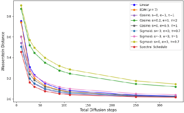
Figure 3: Wasserstein-2 distance comparison between the spectral recommendation and Cosine, Sigmoid, EDM and linear schedules where $d=50$, $l=0.1$, $\boldsymbol{\mu_{0}}=0.05\!\cdot\!\mathbf{1}_{d}$, and the number of diffusion steps considered are $\{10,28,38,60,90,112,250,334\}$.

We also compare our optimal solution with those from previous works. Specifically, Sabour et al. (2024) derives a closed-form expression for the optimal noise schedule under a simplified case, where the initial distribution is an isotropic Gaussian with a standard deviation of $C$, $i.e~\mathbf{x}_{0}\sim\mathcal{N}(\boldsymbol{0},C^{2}\mathbf{I})$. To enable a proper comparison, we frame our optimization problem using the Kullback-Leibler divergence $D_{\mathrm{KL}}$ loss (4.2) as done in (Sabour et al., 2024).

Figure 4 compares our optimal solution, obtained by numerically solving Equation (15), with the closed-form solution from Sabour et al. (2024). It can be observed that both methods align for arbitrary values of $C$. Notably, for $C=1$, both noise schedules converge exactly to the Cosine $(0,1,1)$ noise schedule, which was originally chosen heuristically (Nichol & Dhariwal, 2021).

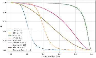
Figure 4: Comparison between the closed-form solution from AYS (Sabour et al., 2024) and our numerical solution for the simplified case where $\mathbf{x}_{0}\sim\mathcal{N}(\boldsymbol{0},C^{2}\mathbf{I})$ with $C=[0.1,0.5,1]$.

Mean drift: The explicit expressions in (11) and (13) offer a further insight into the diffusion process. A notable consideration is whether this process introduces a bias, i.e. drifting the mean component during synthesis. To study this, we analyze the mean bias expression for DDIM, $(\mathbf{D}_{2}-\mathbf{I})\boldsymbol{\mu_{0}^{\mathcal{F}}}$ derived from the difference between $\mathbb{E}\left[\mathbf{\mathbf{x}}_{0}^{\mathcal{F}}\right]$ and $\mathbb{E}\left[\mathbf{\hat{\mathbf{x}}}_{0}^{\mathcal{F}}\right]$. In Appendix K, we further explore the relationship between the target signal characteristics $\left\{\lambda_{i}\right\}_{i=1}^{d}$, the noise schedule $\bar{\boldsymbol{\alpha}}$, and the expression $|\mathbf{D}_{2}-\mathbf{I}|$. It appears that different choices of the noise schedule influence the bias value, with some choices effectively mitigating it. Additionally, as the depth of the diffusion process increases, the bias value tends to grow, regardless of the selected noise schedule.

DDPM vs DDIM: The explicit formulations of DDPM and DDIM in (13) and (11) also enable their comparison in terms of loss across varying diffusion depths and noise schedules. Figure 5 presents such a comparison using the Wasserstein-2 distance on a logarithmic scale. The results clearly expose the fact that DDIM sampling is faster and yields lower loss values, aligning with the empirical observations in Song et al. (2021a).

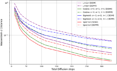
Figure 5: Comparison of the Wasserstein-2 distance between DDPM and DDIM for different noise schedules, including the spectral recommendation, across various diffusion steps.

6.2 Scenario 2: Practical considerations

Sec. 6.1 assumes a synthetic Gaussian distribution. We now shift towards a more practical scenario in which we refer to real data, while still maintaining the Gaussianity assumption. Specifically, we work with signals from the MUSIC dataset (Moura et al., 2020), which consists of recordings of various musical instruments, all down-sampled to $16$kHz. We fit a Gaussian distribution to this data by estimating the mean vector and the circulant covariance matrix of extracted piano-only recordings. This dataset is referred to hereafter as Gaussian MUSIC piano dataset.

The covariance matrix is estimated by using a sliding window of length $d=400$ ($0.025$ seconds) from the original dataset, excluding those with an $L_{1}$ energy below a specified threshold ($th=0.05$) so as to mitigate the influence of silent regions in the covariance estimation. The resulting covariance matrix is symmetric and nearly a Toeplitz matrix. To satisfy the Circulancy assumption, it is approximated as a circulant matrix using the approach discussed in Appendix M. A detailed discussion on the influence of selecting $d$ and $th$ is provided in Appendix I.3.

Figure 6 compares the spectral recommendation derived from the estimated covariance matrix using the Wasserstein-2 distance with various heuristic noise schedules. While the optimal noise schedule retains some resemblance to the hand-crafted approaches, it introduces a somewhat different design of slower decay at the beginning, adapting to the unique dataset’s properties. This is reflected in the estimated parameters, which generally align with the Cosine and Sigmoid functions but feature less conventional values. Consequently, adopting a spectral analysis perspective enables the design of noise schedules tailored to specific needs. Further details, including the spectral recommendation for the SC09 (Warden, 2018) dataset, are provided in Appendix I.

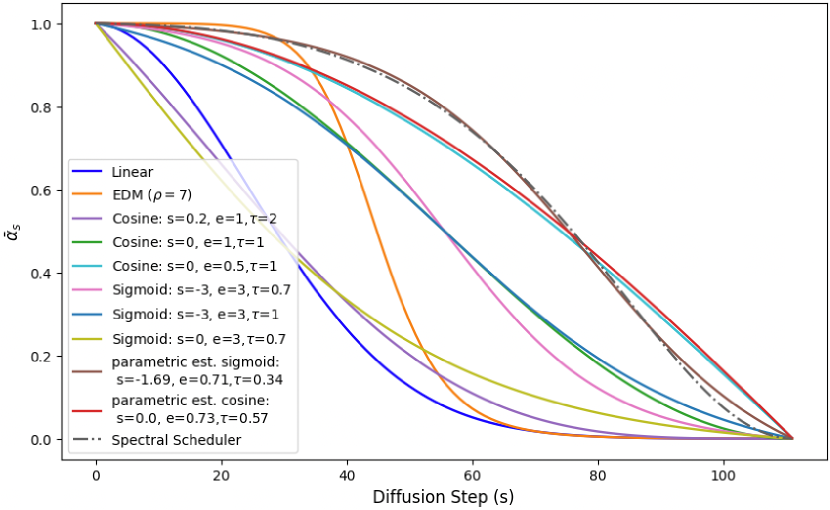
Figure 6: Comparison of the spectral schedule with various heuristic noise schedules for $S=112$ diffusion steps. The best fitted parametric estimations for the Cosine and Sigmoid schedules are presented in red and brown respectively.

6.3 Scenario 3: Into the wild

We now aim to evaluate whether the optimized noise schedule from Sec. 6.2 remains effective when the Gaussianity assumption is removed, and a trained neural denoiser is employed within the diffusion process. The goal in this experiment is to assess the relevance and applicability of the spectral recommendation in more practical scenarios.

Our approach towards performance assessment of different noise schedules is the following: We run the diffusion process as is (with the trained denoiser), and obtain a large corpus of generated signals. We compare the statistics of these synthesized signals to the statistics of true ones, by computing the distance between the second moment of their distribution. The evaluation we employ uses two metrics: the Wasserstein-2 distance and the Frobenius-norm, calculated between the empirical covariance matrices.

Figure 7 compares between the spectral recommendation and heuristic noise schedules. For each schedule, 1,000 signals of length $d=400$ are synthesized using a trained model for each tested number of diffusion steps. The model, based on the architecture presented in (Kong et al., 2021; Benita et al., 2024), employs a linear noise schedule (Ho et al., 2020) with $T=1000$ diffusion steps during training. The training dataset consists of the original piano-only recordings from the MUSIC dataset.

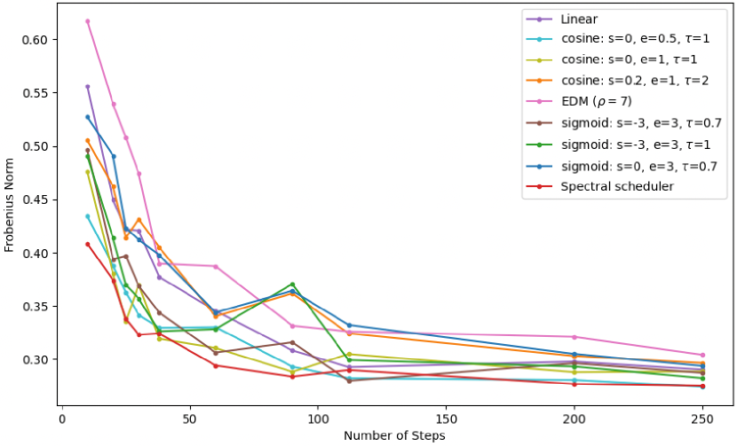
(a)

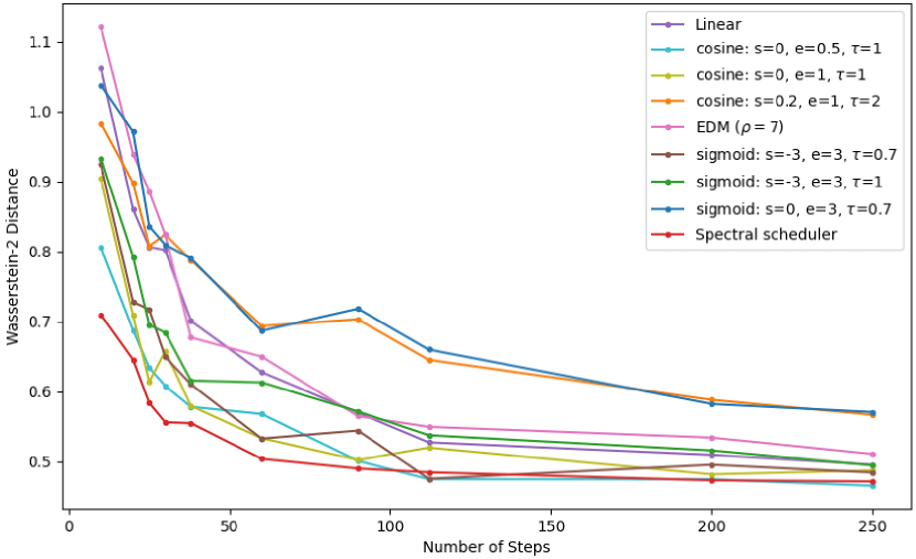
(b)

Figure 7: Figures 7(a) and 7(b) visualize the Frobenius norm and the Wasserstein distance of the spectral noise schedule (in red) compared to existing heuristics, considering the following diffusion steps: $\{10,20,28,30,38,60,90,112,200,250\}$.

As evident from Figure 7, the spectral recommendation consistently outperforms the other noise schedule heuristics in both metrics, with the gap narrowing as the number of diffusion steps grows and the influence of discretization error wanes. Notably, the heuristic Cosine ($0$, $0.5$, $1$), which closely resembles the spectral noise schedule, also performs well, as does Cosine ($0$, $1$, $1$). This suggests that the spectral recommendation effectively preserves the dataset’s key properties even in practical scenarios.

6.4 Further Discussion

Appendix J.1 explores the relationship between the eigenvalue magnitudes and the derived schedule’s structure. A key finding is that large eigenvalues lead to convex schedules that are densely concentrated at the beginning of the diffusion process, whereas small ones result in concave behavior which is more delayed toward the end of the process.

Notably, under the shift-invariance assumption, the eigenvalues directly correspond to the system’s frequency components. In scenarios where the frequency components follow a monotonically decreasing distribution (e.g., the $1/f$ behavior observed in speech (Voss & Clarke, 1975)), the first eigenvalues correspond to the low frequencies, having larger amplitudes, while the last correspond to high frequencies and smaller amplitudes. This pattern, along, with the previous observations, aligns with the well-known coarse-to-fine signal construction behavior of diffusion models.

By recognizing how the eigenvalues shape the noise schedule, we can refine the loss term to better align with our needs. In Appendix J.2 we introduce a weighted-l1 loss, which seem to lead to the well-known Cosine (0,1,1) heuristic, which promotes low frequencies while sacrificing high ones. This highlights how spectral analysis can not only explain noise schedule choices, but also guide the development of more tailored designs.

7 Conclusion

This paper presents a spectral perspective on the inference process in diffusion models. Under the assumptions of Gaussianity and shift invariance, we establish a direct link between the input white noise and the output signal. Our approach enables noise schedule design based on dataset characteristics, diffusion steps, and sampling methods. Effective in synthetic and more realistic settings, the optimized schedules resemble existing heuristics, offering insights on handcrafted design choices. We hope this work encourages further exploration of diffusion models via spectral analysis.

Impact Statement

This paper presents work whose goal is to advance the field of Machine Learning. There are many potential societal consequences of our work, none which we feel must be specifically highlighted here.

Appendix A The Optimal Denoiser for a Gaussian Input

This appendix provides the derivation and explanation of Theorem 3.1.

Let $\mathbf{x}_{0}\sim\mathcal{N}(\boldsymbol{\mu}_{0},\boldsymbol{\Sigma}_{0})$ represent the distribution of the original dataset, where $\mathbf{x}_{0}\in\mathbb{R}^{d}$ . The probability density function $f(\mathbf{x}_{0})$ can be written as:

$$f(\mathbf{x}_{0})=\frac{1}{\sqrt{\left(2\pi\right)^{d}|\boldsymbol{\Sigma}_{0}|}}\cdot\exp\left\{-\frac{1}{2}\left(\bar{\mathbf{x}}_{0}-\bar{\boldsymbol{\mu}}_{0}\right)^{T}{\boldsymbol{\Sigma}}_{0}^{-1}\left(\bar{\mathbf{x}}_{0}-\bar{\boldsymbol{\mu}}_{0}\right)\right\}$$

Through the diffusion process, the signal undergoes noise contamination, leading to the following marginal expression for $\mathbf{x}_{t}$:

$$\mathbf{x}_{t}=\sqrt{\bar{\alpha}_{t}}\mathbf{x}_{0}+\sqrt{1-\bar{\alpha}_{t}}\boldsymbol{\epsilon}~~~~~\boldsymbol{\epsilon}\sim\mathcal{N}(\mathbf{0},\mathbf{I})$$ (18)

For the Maximum A Posteriori (MAP) estimation, we seek to maximize the posterior distribution:

$$\underset{x_{0}}{\max}\log p(\mathbf{x}_{0}|\mathbf{x}_{t})$$

Using Bayes’ rule, this can be written as:

$$\underset{x_{0}}{\min}\,-\log\left[\frac{p(\mathbf{x}_{t}|\mathbf{x}_{0})p(\mathbf{x}_{0})}{p(\mathbf{x}_{t})}\right]=\underset{x_{0}}{\min}\,-\log p(\mathbf{x}_{t}|\mathbf{x}_{0})-\log p(\mathbf{x}_{0})$$ (19)

The conditional likelihood $\log{p(\mathbf{x}_{t}|\mathbf{x}_{0})}$ is given by:

$$p(\mathbf{x}_{t}|\mathbf{x}_{0})=\frac{1}{\sqrt{\left(2\pi\right)^{d}|\Sigma_{1}|)}}\exp\left\{-\frac{1}{2}\left(\mathbf{x}_{t}-\sqrt{\bar{\alpha}_{t}}\mathbf{x}_{0}\right)^{T}\left((1-\bar{\alpha}_{t})\mathbf{I}\right)^{-1}\left(\mathbf{x}_{t}-\sqrt{\bar{\alpha}_{t}}\mathbf{x}_{0}\right)\right\}$$

$$\log\,p(\mathbf{x}_{t}|\mathbf{x}_{0})=-\frac{1}{2}\log{\left(2\pi\right)^{d}|\Sigma_{1}|}-\frac{1}{2(1-\bar{\alpha}_{t})}\left(\mathbf{x}_{t}-\sqrt{\bar{\alpha}_{t}}\mathbf{x}_{0}\right)^{T}\left(\mathbf{x}_{t}-\sqrt{\bar{\alpha}_{t}}\mathbf{x}_{0}\right)$$

The conditional likelihood $\log{p(\mathbf{x}_{0})}$ is given by:

$$p(\mathbf{x}_{0})=\frac{1}{\sqrt{\left(2\pi\right)^{d}|\boldsymbol{\Sigma}_{0}|)}}\exp\left\{-\frac{1}{2}\left(\mathbf{x}_{0}-\boldsymbol{\mu}_{0}\right)^{T}\boldsymbol{\Sigma}_{0}^{-1}\left(\mathbf{x}_{0}-\boldsymbol{\mu}_{0}\right)\right\}$$

$$\log{p(\mathbf{x}_{0})}=-\frac{1}{2}\log{\left(2\pi\right)^{d}|\boldsymbol{\Sigma}_{0}|}-\frac{1}{2}\left(\mathbf{x}_{0}-\boldsymbol{\mu}_{0}\right)^{T}\boldsymbol{\Sigma}_{0}^{-1}\left(\mathbf{x}_{0}-\boldsymbol{\mu}_{0}\right)$$

We will differentiate the given expression in (19) with respect to $x_{0}$ and equate it to zero:

$$\frac{d\log{p(\mathbf{x}_{t}|\mathbf{x}_{0})}}{d\mathbf{x}_{0}}=\frac{2\sqrt{\bar{\alpha}_{t}}\left(\mathbf{x}_{t}-\sqrt{\bar{\alpha}_{t}}\mathbf{x}_{0}\right)}{2(1-\bar{\alpha}_{t})}$$

$$\frac{d\log{p(\mathbf{x}_{0})}}{d\mathbf{x}_{0}}=-\frac{2\boldsymbol{\Sigma}_{0}^{-1}\left(\mathbf{x}_{0}-\boldsymbol{\mu}_{0}\right)}{2}$$

$$\frac{-2\sqrt{\bar{\alpha}_{t}}\left(\mathbf{x}_{t}-\sqrt{\bar{\alpha}_{t}}\mathbf{x}_{0}\right)}{2(1-\bar{\alpha}_{t})}+\frac{2{\boldsymbol{\Sigma}}_{0}^{-1}\left(\mathbf{x}_{0}-\boldsymbol{\mu}_{0}\right)}{2}=0$$

This simplifies to:

$$\frac{-\sqrt{\bar{\alpha}_{t}}\left(\mathbf{x}_{t}-\sqrt{\bar{\alpha}_{t}}\mathbf{x}_{0}\right)}{(1-\bar{\alpha}_{t})}+{\boldsymbol{\Sigma}}_{0}^{-1}\left(\bar{\mathbf{x}}_{0}-\boldsymbol{\mu}_{0}\right)=0$$

Resulting in:

$$-\sqrt{\bar{\alpha}_{t}}{\boldsymbol{\Sigma}}_{0}\mathbf{x}_{t}+\bar{\alpha}_{t}{\boldsymbol{\Sigma}}_{0}\mathbf{x}_{0}+(1-\bar{\alpha}_{t})\mathbf{x}_{0}-(1-\bar{\alpha}_{t})\boldsymbol{\mu}_{0}=0$$

Thus:

$$\left(\bar{\alpha}_{t}{\boldsymbol{\Sigma}}_{0}+(1-\bar{\alpha}_{t})\mathbf{I}\right)\mathbf{x}_{0}=\sqrt{\bar{\alpha}_{t}}{\boldsymbol{\Sigma}}_{0}\mathbf{x}_{t}+(1-\bar{\alpha}_{t})\boldsymbol{\mu}_{0}$$

Finally:

$$\mathbf{x}_{0}^{*}=\left(\bar{\alpha}_{t}{\boldsymbol{\Sigma}}_{0}+(1-\bar{\alpha}_{t})\mathbf{I}\right)^{-1}\left(\sqrt{\bar{\alpha}_{t}}{\boldsymbol{\Sigma}}_{0}\mathbf{x}_{t}+(1-\bar{\alpha}_{t})\boldsymbol{\mu}_{0}\right)$$ (20)

Appendix B The Reverse Process in the Time Domain

Here, we present the reverse process in the time domain for the DDIM (Song et al., 2021a), as outlined in Lemma 3.2.

Let $\mathbf{x}_{0}$ follow the distribution:

$$\mathbf{x}_{0}\sim\mathcal{N}(\boldsymbol{\mu}_{0},\boldsymbol{\Sigma}_{0}),\quad\mathbf{x}_{0}\in\mathbb{R}^{d}$$

Using the procedure outline in (Song et al., 2021a), the diffusion process begins with $\mathbf{x}_{S}\sim\mathcal{N}(\boldsymbol{0},\mathbf{I})$, where $\mathbf{x}_{S}\in\mathbb{R}^{d}$ and progresses through an iterative denoising process described as follows:

$$\mathbf{x}_{s-1}(\eta)=\sqrt{\bar{\alpha}_{s-1}}\left(\frac{\mathbf{x}_{s}-\sqrt{1-\bar{\alpha}_{s}}\cdot\boldsymbol{\epsilon}_{\theta}(\mathbf{x}_{s},s)}{\sqrt{\bar{\alpha}_{s}}}\right)+\sqrt{1-\bar{\alpha}_{s-1}-\sigma_{s}^{2}(\eta)}\cdot\boldsymbol{\epsilon}_{\theta}(\mathbf{x}_{s},s)+\sigma_{s}(\eta)\mathbf{z}_{s}$$ (21)

where

$$\sigma_{s}(\eta)=\eta\sqrt{\frac{1-\bar{\alpha}_{{s-1}}}{1-\bar{\alpha}_{s}}}\sqrt{1-\frac{\bar{\alpha}_{s}}{\bar{\alpha}_{{s-1}}}}$$ (22)

Substituting the marginal property from (2):

$$\boldsymbol{\epsilon}_{\theta}(\mathbf{x}_{s},s)=\frac{\mathbf{x}_{s}-\sqrt{{\bar{\alpha}}_{s}}\hat{\mathbf{x}}_{0}}{\sqrt{1-\bar{\alpha}_{s}}}\quad\quad\hat{\mathbf{x}}_{0}=\frac{\mathbf{x}_{s}-\sqrt{1-\bar{\alpha}_{s}}\cdot\boldsymbol{\epsilon}_{\theta}(\mathbf{x}_{s},s)}{\sqrt{\bar{\alpha}_{s}}}$$ (23)

$$\mathbf{x}_{s-1}(\eta)=\sqrt{\bar{\alpha}_{s-1}}\hat{\mathbf{x}}_{0}+\sqrt{1-\bar{\alpha}_{s-1}-\sigma_{s}^{2}(\eta)}\left(\frac{\mathbf{x}_{s}-\sqrt{{\bar{\alpha}}_{s}}\hat{\mathbf{x}}_{0}}{\sqrt{1-\bar{\alpha}_{s}}}\right)+\sigma_{s}(\eta)\mathbf{z}_{s}$$ (24)

For the deterministic scenario, we choose $\eta=0$ in (22) and obtain $\sigma_{s}(\eta=0)=0$. Therefore:

$$\mathbf{x}_{s-1}(\eta=0) =\sqrt{\bar{\alpha}_{s-1}}\hat{\mathbf{x}}_{0}+\sqrt{1-\bar{\alpha}_{s-1}}\left(\frac{\mathbf{x}_{s}-\sqrt{{\bar{\alpha}}_{s}}\hat{\mathbf{x}}_{0}}{\sqrt{1-\bar{\alpha}_{s}}}\right)$$

$$=\frac{\sqrt{1-\bar{\alpha}_{s-1}}}{\sqrt{1-\bar{\alpha}_{s}}}\mathbf{x}_{s}+\left[\sqrt{\bar{\alpha}_{s-1}}-\frac{\sqrt{{\bar{\alpha}}_{s}}\sqrt{1-\bar{\alpha}_{s-1}}}{\sqrt{1-\bar{\alpha}_{s}}}\right]\hat{\mathbf{x}}_{0}$$ (25)

We denote the following:

$$a_{s}=\frac{\sqrt{1-\bar{\alpha}_{s-1}}}{\sqrt{1-\bar{\alpha}_{s}}}\quad\quad b_{s}=\sqrt{\bar{\alpha}_{s-1}}-\frac{\sqrt{{\bar{\alpha}}_{s}}\sqrt{1-\bar{\alpha}_{s-1}}}{\sqrt{1-\bar{\alpha}_{s}}}$$

Therefore we get the following equation:

$$\mathbf{x}_{s-1}=a_{s}\mathbf{x}_{s}+b_{s}\mathbf{x}_{0}^{*}~.$$

Using the result from the MAP estimator:

$$\mathbf{x}_{0}^{*}=\left(\bar{\alpha}_{s}\boldsymbol{\Sigma}_{0}+(1-\bar{\alpha}_{s})\mathbf{I}\right)^{-1}\left(\sqrt{\bar{\alpha}_{s}}\boldsymbol{\Sigma}_{0}\mathbf{x}_{t}+(1-\bar{\alpha}_{s})\boldsymbol{\mu}_{0}\right)$$

we get:

$$\mathbf{x}_{s-1}=a_{s}\mathbf{x}_{s}+b_{s}\left(\bar{\alpha}_{s}{\boldsymbol{\Sigma}}_{0}+(1-\bar{\alpha}_{s})\mathbf{I}\right)^{-1}\left(\sqrt{\bar{\alpha}_{s}}{\boldsymbol{\Sigma}}_{0}\mathbf{x}_{s}+(1-\bar{\alpha}_{s})\boldsymbol{\mu}_{0}\right)$$

$$\mathbf{x}_{s-1}=\left(a_{s}+b_{s}\left(\bar{\alpha}_{s}{\boldsymbol{\Sigma}}_{0}+(1-\bar{\alpha}_{s})\mathbf{I}\right)^{-1}\sqrt{\bar{\alpha}_{s}}{\boldsymbol{\Sigma}}_{0}\right)\mathbf{x}_{s}+\left(b_{s}\left(\bar{\alpha}_{s}{\boldsymbol{\Sigma}}_{0}+(1-\bar{\alpha}_{s})\mathbf{I}\right)^{-1}(1-\bar{\alpha}_{s})\boldsymbol{\mu}_{0}\right)$$ (26)

Introduce the notation:

$$\bar{\boldsymbol{\Sigma}}_{0,s}=\bar{\alpha}_{s}{\boldsymbol{\Sigma}}_{0}+(1-\bar{\alpha}_{s})\mathbf{I}$$

We can rewrite the equation as:

$$\mathbf{x}_{s-1}=\left(a_{s}\mathbf{I}+b_{s}\sqrt{\bar{\alpha}_{s}}\left(\bar{\boldsymbol{\Sigma}}_{0,s}\right)^{-1}{\boldsymbol{\Sigma}}_{0}\right)\mathbf{x}_{s}+b_{s}\left(1-\bar{\alpha}_{s}\right)\left(\bar{\boldsymbol{\Sigma}}_{0,s}\right)^{-1}\boldsymbol{\mu_{0}}$$ (27)

Appendix C Migrating to the Spectral Domain

Here, we demonstrate the application of the Discrete Fourier Transform (DFT), denoted by $\mathcal{F}\{\cdot\}$, to both sides of Eq. (7), as outlined in Lemma 3.3. At this stage, we assume that the covariance matrix $\boldsymbol{\Sigma}_{0}$ is circulant, as it allows us to derive a closed analytical solution. We apply the DFT by multiplying both sides of the equation by the Fourier matrix $\mathbf{F}$:

$$\mathbf{F}\mathbf{x}_{s-1}=\mathbf{F}\left[\left(a_{s}\mathbf{I}+b_{s}\sqrt{\bar{\alpha}_{s}}\bar{\boldsymbol{\Sigma}}^{-1}_{0,s}\boldsymbol{\Sigma}_{0}\right)\mathbf{x}_{s}+b_{s}(1-\bar{\alpha}_{s})\bar{\boldsymbol{\Sigma}}^{-1}_{0,s}\boldsymbol{\mu_{0}}\right]$$ (28)

$$\mathbf{x}^{\mathcal{F}}_{s-1}=a_{s}\mathbf{x}^{\mathcal{F}}_{s}+\mathbf{F}b_{s}\sqrt{\bar{\alpha}_{s}}\bar{\boldsymbol{\Sigma}}_{0,s}^{-1}\mathbf{F}^{T}\mathbf{F}{\boldsymbol{\Sigma}}_{0}\mathbf{F}^{T}\mathbf{F}\mathbf{x}_{s}+\mathbf{F}b_{s}(1-\bar{\alpha}_{s})\bar{\boldsymbol{\Sigma}}_{0,s}^{-1}\mathbf{F}^{T}\mathbf{F}\boldsymbol{\mu_{0}}$$

$$\mathbf{x}^{\mathcal{F}}_{s-1}=a_{s}\mathbf{x}^{\mathcal{F}}_{s}+b_{s}\sqrt{\bar{\alpha}_{s}}\mathbf{F}\bar{\boldsymbol{\Sigma}}_{0,s}^{-1}\mathbf{F}^{T}\mathbf{F}{\boldsymbol{\Sigma}}_{0}\mathbf{F}^{T}\mathbf{x}^{\mathcal{F}}_{s}+b_{s}(1-\bar{\alpha}_{s})\mathbf{F}\bar{\boldsymbol{\Sigma}}_{0,s}^{-1}\mathbf{F}^{T}\boldsymbol{\mu_{0}}^{\mathcal{F}}$$

Assuming circulancy, the matrix $\boldsymbol{\Sigma}_{0}$ can be diagonalized by the DFT matrix:

• $\mathbf{F}\boldsymbol{\Sigma}_{0}\mathbf{F}^{T}=\mathbf{\Lambda}_{0}$,  $\mathbf{F}^{T}\mathbf{\Lambda}_{0}\mathbf{F}=\boldsymbol{\Sigma}_{0}$

• $a\boldsymbol{\Sigma}_{0}+b\mathbf{I}=a\mathbf{F}^{T}\mathbf{\Lambda}_{0}\mathbf{F}+b\mathbf{F}^{T}\mathbf{I}\mathbf{F}=\mathbf{F}^{T}\left(a\mathbf{\Lambda}_{0}+b\mathbf{I}\right)\mathbf{F}$

• $\mathbf{F}\boldsymbol{\Sigma}_{0}^{-1}\mathbf{F}^{T}=\mathbf{\Lambda}_{0}^{-1}$,  $\mathbf{F}^{T}\mathbf{\Lambda}_{0}^{-1}\mathbf{F}=\boldsymbol{\Sigma}_{0}^{-1}$

Therefore, we obtain:

$$\mathbf{F}\bar{\boldsymbol{\Sigma}}_{0,s}^{-1}\mathbf{F}^{T}=\mathbf{F}\left[\bar{\alpha}_{s}\boldsymbol{\Sigma}_{0}+(1-\bar{\alpha}_{s})\mathbf{I}\right]^{-1}\mathbf{F}^{T}=\left[\bar{\alpha}_{s}\mathbf{\Lambda}_{0}+(1-\bar{\alpha}_{s})\mathbf{I}\right]^{-1}$$

Including those elements in the main equation:

$$\mathbf{x}_{s-1}^{\mathcal{F}}=\left[a_{s}+b_{s}\sqrt{\bar{\alpha}_{s}}\left[\bar{\alpha}_{s}\mathbf{\Lambda}_{0}+(1-\bar{\alpha}_{s})\mathbf{I}\right]^{-1}\mathbf{\Lambda}_{0}\right]\mathbf{x}_{s}^{\mathcal{F}}+b_{s}(1-\bar{\alpha}_{s})\left[\bar{\alpha}_{s}\mathbf{\Lambda}_{0}+(1-\bar{\alpha}_{s})\mathbf{I}\right]^{-1}\boldsymbol{\mu_{0}}^{\mathcal{F}}$$

We will denote the following:

$$\mathbf{G}(s)=\left[a_{s}+b_{s}\sqrt{\bar{\alpha}_{s}}\left[\bar{\alpha}_{s}\mathbf{\Lambda}_{0}+(1-\bar{\alpha}_{s})\mathbf{I}\right]^{-1}\mathbf{\Lambda}_{0}\right]$$

$$\mathbf{M}(s)=b_{s}(1-\bar{\alpha}_{s})\left[\bar{\alpha}_{s}\mathbf{\Lambda}_{0}+(1-\bar{\alpha}_{s})\mathbf{I}\right]^{-1}$$

and get:

$$\mathbf{x}_{s-1}^{\mathcal{F}}=\mathbf{G}(s)\mathbf{x}_{s}^{\mathcal{F}}+\mathbf{M}(s)\boldsymbol{\mu_{0}}^{\mathcal{F}}$$ (29)

We can then recursively obtain $\mathbf{x}_{l}^{\mathcal{F}}$ for a general $l$:

$$\mathbf{x}_{l}^{\mathcal{F}}=\left[\prod_{s^{{}^{\prime}}=l+1}^{S}\mathbf{G}(s^{{}^{\prime}})\right]\mathbf{x}_{S}^{\mathcal{F}}+\left[\sum_{i=l+1}^{S}\left(\prod_{j=l+1}^{i-1}\mathbf{G}(j)\right)\mathbf{M}(i)\right]\boldsymbol{\mu_{0}}^{\mathcal{F}}$$

specifically for $l=0$:

$$\mathbf{\hat{x}}_{0}^{\mathcal{F}}=\left[\prod_{s^{{}^{\prime}}=1}^{S}\mathbf{G}(s^{{}^{\prime}})\right]\mathbf{x}_{S}^{\mathcal{F}}+\left[\sum_{i=1}^{S}\left(\prod_{j=1}^{i-1}\mathbf{G}(j)\right)\mathbf{M}(i)\right]\boldsymbol{\mu_{0}}^{\mathcal{F}}$$

We will denote the following:

$$\mathbf{D}_{1}=\prod_{s=1}^{S}\mathbf{G}(s)=\prod_{s=1}^{S}\left[a_{s}+b_{s}\sqrt{\bar{\alpha}_{s}}\left[\bar{\alpha}_{s}\mathbf{\Lambda}_{0}+\mathbf{I}(1-\bar{\alpha}_{s})\right]^{-1}\mathbf{\Lambda}_{0}\right]$$ (30)

$$\mathbf{D}_{2}=\sum_{i=1}^{S}\left(\prod_{j=1}^{i-1}\mathbf{G}(j)\right)\mathbf{M}(i)=\sum_{i=1}^{S}\left[\left(\prod_{j=1}^{i-1}\left[a_{j}+b_{j}\sqrt{\bar{\alpha}_{j}}\left[\bar{\alpha}_{j}\mathbf{\Lambda}_{0}+\mathbf{I}(1-\bar{\alpha}_{j})\right]^{-1}\mathbf{\Lambda}_{0}\right]\right)b_{i}(1-\bar{\alpha}_{i})\left[\bar{\alpha}_{i}\mathbf{\Lambda}_{0}+\mathbf{I}(1-\bar{\alpha}_{i})\right]^{-1}\right]$$ (31)

Substitute $D_{1}$ and $D_{2}$ into the last equation, we get:

$$\mathbf{\hat{x}}_{0}^{\mathcal{F}}=\mathbf{D}_{1}\mathbf{x}_{S}^{\mathcal{F}}+\mathbf{D}_{2}\boldsymbol{\mu_{0}}^{\mathcal{F}}$$ (32)

The resulting vector from Equation 32 is a linear combination of Gaussian signals, therefore it also follows a Gaussian distribution. We now aim to determine the mean and covariance of that distribution.

$$\mathbf{\hat{\mathbf{x}}^{\mathcal{F}}}_{0}\sim\mathcal{N}(\mathbb{E}\left[\mathbf{\hat{\mathbf{x}}}_{0}^{\mathcal{F}}\right],\mathbf{\Sigma}_{\mathbf{\hat{\mathbf{x}}}_{0}^{\mathcal{F}}}),\quad\mathbf{\hat{\mathbf{x}}}_{0}^{\mathcal{F}}\in\mathbb{R}^{d}$$

Mean:

$$\mathbb{E}\left[\mathbf{\hat{\mathbf{x}}}_{0}^{\mathcal{F}}\right]=\mathbb{E}\left[\mathbf{D}_{1}\mathbf{x}_{S}^{\mathcal{F}}+\mathbf{D}_{2}\boldsymbol{\mu}_{0}^{\mathcal{F}}\right]=\mathbf{D}_{1}\mathbf{F}\mathbb{E}\left[\mathbf{\mathbf{x}}_{S}\right]+\mathbb{E}\left[\mathbf{D}_{2}\boldsymbol{\mu}_{0}^{\mathcal{F}}\right]=\mathbf{D}_{2}\boldsymbol{\mu}_{0}^{\mathcal{F}}$$

$$\mathbf{\mathbf{x}}_{S}\sim\mathcal{N}(\boldsymbol{0},\mathbf{I})$$

$$\mathbb{E}\left[\mathbf{\hat{x}}_{0}^{\mathcal{F}}\right]=\mathbf{D}_{2}\boldsymbol{\mu}_{0}^{\mathcal{F}}$$

Covariance:

$$\mathbf{\Sigma}_{\mathbf{\hat{x}}_{0}^{\mathcal{F}}}=\mathbb{E}\left[\left(\mathbf{D}_{1}\mathbf{x}_{S}^{\mathcal{F}}+\mathbf{D}_{2}F\boldsymbol{\mu_{0}}-\mathbb{E}\left[\mathbf{D}_{1}\mathbf{x}_{S}^{\mathcal{F}}+\mathbf{D}_{2}F\boldsymbol{\mu_{0}}\right]\right)\left(\mathbf{D}_{1}\mathbf{x}_{S}^{\mathcal{F}}+\mathbf{D}_{2}F\boldsymbol{\mu_{0}}-\mathbb{E}\left[\mathbf{D}_{1}\mathbf{x}_{S}^{\mathcal{F}}+\mathbf{D}_{2}F\boldsymbol{\mu_{0}}\right]\right)^{T}\right]$$

$$=\mathbb{E}\left[\left(\mathbf{D}_{1}\mathbf{x}_{S}^{\mathcal{F}}+\mathbf{D}_{2}F\boldsymbol{\mu_{0}}-\mathbf{D}_{2}F\boldsymbol{\mu_{0}}\right)\left(D_{1}\mathbf{x}_{S}^{\mathcal{F}}+\mathbf{D}_{2}F\boldsymbol{\mu_{0}}-D_{2}F\boldsymbol{\mu_{0}}\right)^{T}\right]$$

$$=\mathbb{E}\left[\left(\mathbf{D}_{1}\mathbf{x}_{S}^{\mathcal{F}}\right)\left(\mathbf{D}_{1}\mathbf{x}_{S}^{\mathcal{F}}\right)^{T}\right]=\mathbf{D}_{1}\mathbb{E}\left[\mathbf{x}_{S}^{\mathcal{F}}\left(\mathbf{x}_{S}^{\mathcal{F}}\right)^{T}\right]{\mathbf{D}_{1}}^{T}$$

$$\mathbf{\Sigma}_{\mathbf{\hat{x}}_{0}^{\mathcal{F}}}=\mathbf{D}_{1}{\mathbf{D}_{1}}^{T}={\mathbf{D}_{1}}^{2}$$

$$\mathbf{\hat{x}}_{0}^{\mathcal{F}}\sim\mathcal{N}(\mathbf{D}_{2}\boldsymbol{\mu_{0}}^{\mathcal{F}},\mathbf{D}_{1}^{2}),\quad\mathbf{\hat{x}}_{0}^{\mathcal{F}}\in\mathbb{R}^{d}.$$ (33)

It should be noted that, for the data distribution $\mathbf{x}_{0}\sim\mathcal{N}(\boldsymbol{\mu}_{0},\boldsymbol{\Sigma}_{0}),~~where\mathbf{x}_{0}\in\mathbb{R}^{d}$, its first and second moments in the frequency domain are defined as follows:

$$\mathbb{E}\left[\mathbf{\mathbf{x}}_{0}^{\mathcal{F}}\right]=\mathbf{F}\mathbb{E}\left[\mathbf{\mathbf{x}}_{0}\right]=\boldsymbol{\mu}_{0}^{\mathcal{F}}$$

$$\Sigma_{\mathbf{x}_{0}^{\mathcal{F}}}=\boldsymbol{\Lambda}_{0}$$

$$\mathbf{x}_{0}^{\mathcal{F}}\sim\mathcal{N}(\boldsymbol{\mu}_{0}^{\mathcal{F}},\boldsymbol{\Lambda}_{0})$$ (34)

Appendix D Evaluating loss functions expressions

Here, we present selected loss functions based on the derivations provided in Section 3.

D.1 Wasserstein-2 Distance:

The Wasserstein-2 distance between two Gaussian distributions with means $\mu_{1}$ and $\mu_{2}$, and covariance matrices $\Sigma_{1}$ and $\Sigma_{2}$, and the corresponding eigenvalues $\{\lambda_{1}^{(i)}\}_{i=1}^{d}$ and $\{\lambda_{2}^{(i)}\}_{i=1}^{d}$ is given by:

$$W_{2}(\mathcal{N}_{1},\mathcal{N}_{2})=\sqrt{(\boldsymbol{\mu}_{1}-\boldsymbol{\mu}_{2})^{T}(\boldsymbol{\mu}_{1}-\boldsymbol{\mu}_{2})+\sum_{i}\left(\sqrt{\lambda_{1}^{(i)}}-\sqrt{\lambda_{2}^{(i)}}\right)^{2}}$$ (35)

$$\text{Since }\quad\mathbf{\hat{x}_{0}^{\mathcal{F}}}\sim\mathcal{N}(\mathbf{D}_{2}\boldsymbol{\mu_{0}}^{\mathcal{F}},\mathbf{D}_{1}^{2}),\quad\mathbf{\hat{x}}_{0}^{\mathcal{F}}\in\mathbb{R}^{d}\quad\text{and}\quad\mathbf{x}_{0}^{\mathcal{F}}\sim\mathcal{N}(\boldsymbol{\mu}_{0}^{\mathcal{F}},\boldsymbol{\Lambda}_{0}),\quad\mathbf{x}_{0}^{\mathcal{F}}\in\mathbb{R}^{d}\quad$$

we obtain:

$$\left(\boldsymbol{\mu}_{1}-\boldsymbol{\mu}_{2}\right)^{T}(\boldsymbol{\mu}1-\boldsymbol{\mu}_{2})=\left(\mathbf{D}_{2}\boldsymbol{\mu}_{0}^{\mathcal{F}}-\boldsymbol{\mu}_{0}^{\mathcal{F}}\right)^{T}\left(\mathbf{D}_{2}\boldsymbol{\mu}_{0}^{\mathcal{F}}-\boldsymbol{\mu}_{0}^{\mathcal{F}}\right)=\left((\boldsymbol{\mu_{0}}^{\mathcal{F}})^{T}\mathbf{D}_{2}^{T}-(\boldsymbol{\mu_{0}}^{\mathcal{F}})^{T}\right)\left(\mathbf{D}_{2}\boldsymbol{\mu}_{0}^{\mathcal{F}}-\boldsymbol{\mu}_{0}^{\mathcal{F}}\right)$$

$$=(\boldsymbol{\mu_{0}}^{\mathcal{F}})^{T}\boldsymbol{\mu_{0}}^{\mathcal{F}}-2(\boldsymbol{\mu_{0}}^{\mathcal{F}})^{T}\mathbf{D}_{2}\boldsymbol{\mu_{0}}^{\mathcal{F}}+(\boldsymbol{\mu_{0}}^{\mathcal{F}})^{T}\mathbf{D}_{2}^{T}\mathbf{D}_{2}\boldsymbol{\mu_{0}}^{\mathcal{F}}$$

$$=\sum_{i=1}^{d}{\left(\boldsymbol{\mu_{0}}^{\mathcal{F}}\right)}_{i}^{2}-2\sum_{i=1}^{d}{\left(\boldsymbol{\mu_{0}}^{\mathcal{F}}\right)}_{i}^{2}{\mathbf{D}_{2}}^{(i)}+\sum_{i=1}^{d}{\left(\boldsymbol{\mu_{0}}^{\mathcal{F}}\right)}_{i}^{2}\left({\mathbf{D}_{2}}^{(i)}\right)^{2}$$

$$=\sum_{i=1}^{d}\left({\mathbf{D}_{2}}^{(i)}-1\right)^{2}{\left(\boldsymbol{\mu_{0}}^{\mathcal{F}}\right)}_{i}^{2}$$

$$\left(\boldsymbol{\mu}_{1}-\boldsymbol{\mu}_{2}\right)^{T}(\boldsymbol{\mu}1-\boldsymbol{\mu}_{2})=\sum_{i=1}^{d}\left({\mathbf{D}_{2}}^{(i)}-1\right)^{2}{\left(\boldsymbol{\mu_{0}}^{\mathcal{F}}\right)}_{i}^{2}$$

$$\sum_{i}\left(\sqrt{\lambda_{1}^{(i)}}-\sqrt{\lambda_{2}^{(i)}}\right)^{2}=\sum_{i}\left(\sqrt{\lambda_{0}^{(i)}}-\sqrt{\left({\mathbf{D}_{1}}^{(i)}\right)^{2}}\right)^{2}$$

$$W_{2}(\mathbf{x}_{0}^{\mathcal{F}},\mathbf{\hat{x}_{0}^{\mathcal{F}}})=\sqrt{\sum_{i=1}^{d}\left({d_{2}}^{(i)}-1\right)^{2}{\left(\boldsymbol{\mu_{0}}^{\mathcal{F}}\right)}_{i}^{2}+\sum_{i}\left(\sqrt{\lambda_{0}^{(i)}}-\sqrt{\left({\mathbf{D}_{1}}^{(i)}\right)^{2}}\right)^{2}}$$ (36)

D.2 Kullback-Leibler divergence:

The Kullback-Leibler (KL) divergence between two Gaussian distributions with means $\mu_{1}$ and $\mu_{2}$, and covariance matrices $\Sigma_{1}$ and $\Sigma_{2}$, and the corresponding eigenvalues $\{\lambda_{1}^{(i)}\}_{i=1}^{d}$ and $\{\lambda_{2}^{(i)}\}_{i=1}^{d}$ is given by:

$$D_{\text{KL}}\left(\mathcal{N}(\mathbf{\mu}_{1},\boldsymbol{\Sigma}_{1})\parallel\mathcal{N}(\mu_{2},\boldsymbol{\Sigma}_{2})\right)=\frac{1}{2}\left(\log\frac{|\boldsymbol{\Sigma}_{2}|}{|\boldsymbol{\Sigma}_{1}|}-d+\operatorname{tr}\left(\boldsymbol{\Sigma}_{2}^{-1}\boldsymbol{\Sigma}_{1}\right)+(\boldsymbol{\mu}_{2}-\boldsymbol{\mu}_{1})^{T}\boldsymbol{\Sigma}_{2}^{-1}(\boldsymbol{\mu}_{2}-\boldsymbol{\mu}_{1})\right)$$

Given:

$$\quad\mathbf{\hat{x}_{0}^{\mathcal{F}}}\sim\mathcal{N}(\mathbf{D}_{2}\boldsymbol{\mu_{0}}^{\mathcal{F}},\mathbf{D}_{1}^{2}),\quad\mathbf{\hat{x}}_{0}^{\mathcal{F}}\in\mathbb{R}^{d}\quad\text{and}\quad\mathbf{x}_{0}^{\mathcal{F}}\sim\mathcal{N}(\boldsymbol{\mu}_{0}^{\mathcal{F}},\boldsymbol{\Lambda}_{0}),\quad\mathbf{x}_{0}^{\mathcal{F}}\in\mathbb{R}^{d}\quad$$

The KL divergence is given by:

$$D_{\text{KL}}\left(\mathbf{x}_{0}^{\mathcal{F}}\parallel\mathbf{\hat{x}}_{0}^{\mathcal{F}}\right)=D_{\text{KL}}\left(\mathcal{N}\left(\mathbb{E}\left[\mathbf{x}_{0}^{\mathcal{F}}\right],\boldsymbol{\Sigma}_{\mathbf{x}_{0}^{\mathcal{F}}}\right),\,\mathcal{N}\left(\mathbb{E}\left[\mathbf{\hat{x}}_{0}^{\mathcal{F}}\right],\boldsymbol{\Sigma}_{\mathbf{\hat{x}}_{0}^{\mathcal{F}}}\right)\right)$$

$$=D_{\text{KL}}\left(\mathcal{N}\left(\boldsymbol{\mu}_{0}^{\mathcal{F}},\mathbf{\Lambda}_{0}\right),\,\mathcal{N}\left(\mathbf{D}_{2}\ \boldsymbol{\mu}_{0}^{\mathcal{F}}{\mathbf{D}_{1}}^{2}\right)\right)$$

By decomposing the KL divergence elements, we obtain the following terms:

• $|\boldsymbol{\Sigma}_{2}|=|\mathbf{D}_{1}^{T}\mathbf{D}_{1}|=|\mathbf{D}_{1}^{2}|=\prod_{i=1}^{d}{\mathbf{D}_{1}^{(i)}}^{2}$

• $|\boldsymbol{\Sigma}_{1}|=\prod_{i=1}^{d}\lambda_{0}^{(i)}$

• $\operatorname{tr}\left(\boldsymbol{\Sigma}_{2}^{-1}\boldsymbol{\Sigma}_{1}\right)=\sum_{i=1}^{d}\frac{\lambda_{0}^{(i)}}{{\mathbf{D}_{1}^{(i)}}^{2}}$

• $(\boldsymbol{\mu}_{2}-\boldsymbol{\mu}_{1})^{T}\boldsymbol{\Sigma}_{2}^{-1}(\boldsymbol{\mu}_{2}-\boldsymbol{\mu}_{1})=(\mathbf{D}_{2}\boldsymbol{\mu}_{0}^{\mathcal{F}}-\boldsymbol{\mu}_{0}^{\mathcal{F}})^{T}\left({{\mathbf{D}_{1}}^{2}}\right)^{-1}(\mathbf{D}_{2}\boldsymbol{\mu}_{0}^{\mathcal{F}}-\boldsymbol{\mu}_{0}^{\mathcal{F}})=$

  $$=\left(\boldsymbol{\mu_{0}}^{\mathcal{F}}\right)^{T}\left(\mathbf{D}_{2}^{T}-I\right)\left({{\mathbf{D}_{1}}^{2}}\right)^{-1}\left(\mathbf{D}_{2}-I\right)\boldsymbol{\mu_{0}}^{\mathcal{F}}=\sum_{i=1}^{d}\frac{\left({\mathbf{D}_{2}}^{(i)}-1\right)^{2}}{{\mathbf{D}_{1}^{(i)}}^{2}}{\left(\boldsymbol{\mu_{0}}^{\mathcal{F}}_{i}\right)}^{2}$$

Applying the substitution, the term results in:

$$D_{\text{KL}}\left(\mathcal{N}\left(\boldsymbol{\mu}_{0}^{\mathcal{F}},\mathbf{\Lambda}_{0}\right),\,\mathcal{N}\left(\mathbf{D}_{2}\boldsymbol{\mu}_{0}^{\mathcal{F}},{\mathbf{D}_{1}}^{2}\right)\right)=$$

$$=\frac{1}{2}\left[\sum_{i=1}^{d}\log{\mathbf{D}_{1}^{(i)}}^{2}-\sum_{i=1}^{d}\log{\lambda_{0}^{(i)}}\ -d+\sum_{i=1}^{d}\frac{\lambda_{0}^{(i)}}{{\mathbf{D}_{1}^{(i)}}^{2}}+\sum_{i=1}^{d}\frac{\left({\mathbf{D}_{2}}^{(i)}-1\right)^{2}}{{\mathbf{D}_{1}^{(i)}}^{2}}{\left(\boldsymbol{\mu_{0}}^{\mathcal{F}}_{i}\right)}^{2}\right]$$

$$D_{\text{KL}}\left(\mathbf{x}_{0}^{\mathcal{F}}\parallel\mathbf{\hat{x}}_{0}^{\mathcal{F}}\right)=\frac{1}{2}\left[\sum_{i=1}^{d}2\log{\mathbf{D}_{1}^{(i)}}-\sum_{i=1}^{d}\log{\lambda_{0}^{(i)}}\ -d+\sum_{i=1}^{d}\frac{\lambda_{0}^{(i)}+\left({\mathbf{D}_{2}}^{(i)}-1\right)^{2}{\left(\boldsymbol{\mu_{0}}^{\mathcal{F}}\right)}_{i}^{2}}{{\mathbf{D}_{1}^{(i)}}^{2}}\right]$$ (37)

Appendix E DDPM Formulation:

Here, we apply an equivalent procedure to the DDPM scenario, as we did for the DDIM, as outlined in Theorem 3.5.

E.1 The Reverse Process in the Time Domain

Using the procedure outline in Ho et al. (2020), the diffusion process begins with $\mathbf{x}_{T}\sim\mathcal{N}(\boldsymbol{0},\mathbf{I})$, where $\mathbf{x}_{T}\in\mathbb{R}^{d}$, and progresses through an iterative denoising process described as follows:

$$\mathbf{x}_{t-1}=\frac{1}{\sqrt{{\alpha}_{t}}}\left(\mathbf{x}_{t}-\frac{1-\alpha_{t}}{\sqrt{1-\bar{\alpha}_{t}}}\boldsymbol{\epsilon}_{\theta}(\mathbf{x}_{t},t)\right)+\sigma_{t}\mathbf{z}_{t}\quad\mathbf{z}_{t}\sim\mathcal{N}(0,I)$$ (38)

Where $\sigma_{t}=\sqrt{\frac{1-\bar{\alpha}_{t-1}}{1-\bar{\alpha}_{t}}(1-\alpha_{t})}$.

Given the marginal property from (2):

$$\boldsymbol{\epsilon}_{\theta}(\mathbf{x}_{t},t)=\frac{\mathbf{x}_{t}-\sqrt{{\bar{\alpha}}_{t}}\hat{\mathbf{x}}_{0}}{\sqrt{1-\bar{\alpha}_{t}}}$$

we can incorporate it into (38):

$$\mathbf{x}_{t-1} = \frac{1}{\sqrt{{\alpha}_{t}}}\left(\mathbf{x}_{t}-\frac{1-\alpha_{t}}{\sqrt{1-\bar{\alpha}_{t}}}\left(\frac{\mathbf{x}_{t}-\sqrt{{\bar{\alpha}}_{t}}\hat{\mathbf{x}}_{0}}{\sqrt{1-\bar{\alpha}_{t}}}\right)\right)+\sigma_{t}\mathbf{z}_{t}$$

$$\mathbf{x}_{t-1} = \frac{1}{\sqrt{{\alpha}_{t}}}\left(\mathbf{x}_{t}\left(1-\frac{1-\alpha_{t}}{1-\bar{\alpha}_{t}}\right)+\frac{\left(1-\alpha_{t}\right)\sqrt{\bar{\alpha}_{t}}}{1-\bar{\alpha}_{t}}\hat{\mathbf{x}}_{0}\right)+\sigma_{t}\mathbf{z}_{t}$$

$$\mathbf{x}_{t-1} = \frac{1}{\sqrt{{\alpha}_{t}}}\left(\frac{\alpha_{t}-\bar{\alpha}_{t}}{1-\bar{\alpha}_{t}}\right)\mathbf{x}_{t}+\sqrt{\frac{\bar{\alpha}_{t}}{\alpha_{t}}}\frac{\left(1-\alpha_{t}\right)}{1-\bar{\alpha}_{t}}\hat{\mathbf{x}}_{0}+\sigma_{t}\mathbf{z}_{t}$$ (39)

We denote the following, where the final term in each equation is represented by $\bar{\alpha}_{t}$ and $\bar{\alpha}_{t-1}$:

$$a_{t}=\frac{1}{\sqrt{{\alpha}_{t}}}\left(\frac{\alpha_{t}-\bar{\alpha}_{t}}{1-\bar{\alpha}_{t}}\right)=\frac{\sqrt{\bar{\alpha}_{t}}}{1-\bar{\alpha}_{t}}\left[\frac{1}{\sqrt{\bar{\alpha}_{t-1}}}-\sqrt{\bar{\alpha}_{t-1}}\right]$$

$$b_{t}=\sqrt{\frac{\bar{\alpha}_{t}}{\alpha_{t}}}\frac{\left(1-\alpha_{t}\right)}{1-\bar{\alpha}_{t}}=\sqrt{\bar{\alpha}_{t-1}}\left(\frac{1-\frac{\bar{\alpha}_{t}}{\bar{\alpha}_{t-1}}}{1-\bar{\alpha}_{t}}\right)$$

$$c_{t}=\sigma_{t}=\sqrt{\frac{1-\bar{\alpha}_{t-1}}{1-\bar{\alpha}_{t}}(1-\alpha_{t})}=\sqrt{\frac{1-\bar{\alpha}_{t-1}}{1-\bar{\alpha}_{t}}\left(1-\frac{\bar{\alpha}_{t}}{\bar{\alpha}_{t-1}}\right)}$$

Therefore we get the following equation:

$$\mathbf{x}_{t-1}=a_{t}\mathbf{x}_{t}+b_{t}\hat{\mathbf{x}}_{0}+c_{t}\mathbf{z}_{t}$$

Using the result for the MAP estimator from (3.1):

$$\mathbf{x}_{0}^{*}=\left(\bar{\alpha}_{t}{\boldsymbol{\Sigma}}_{0}+(1-\bar{\alpha}_{t})\mathbf{I}\right)^{-1}\left(\sqrt{\bar{\alpha}_{t}}{\boldsymbol{\Sigma}}_{0}\mathbf{x}_{t}+(1-\bar{\alpha}_{t})\boldsymbol{\mu}_{0}\right)$$

we get:

$$\mathbf{x}_{t-1}=a_{t}\mathbf{x}_{t}+b_{t}\left(\bar{\alpha}_{t}{\boldsymbol{\Sigma}}_{0}+(1-\bar{\alpha}_{t})\mathbf{I}\right)^{-1}\left(\sqrt{\bar{\alpha}_{t}}{\boldsymbol{\Sigma}}_{0}\mathbf{x}_{t}+(1-\bar{\alpha}_{t})\boldsymbol{\mu}_{0}\right)+c_{t}\mathbf{z}_{t}$$

$$\mathbf{x}_{t-1}=\left(a_{t}+b_{t}\left(\bar{\alpha}_{t}{\boldsymbol{\Sigma}}_{0}+(1-\bar{\alpha}_{t})\mathbf{I}\right)^{-1}\sqrt{\bar{\alpha}_{t}}{\boldsymbol{\Sigma}}_{0}\right)\mathbf{x}_{t}+\left(b_{t}\left(\bar{\alpha}_{t}{\boldsymbol{\Sigma}}_{0}+(1-\bar{\alpha}_{t})\mathbf{I}\right)^{-1}(1-\bar{\alpha}_{t})\boldsymbol{\mu}_{0}\right)+c_{t}\mathbf{z}_{t}$$

Using the notation from Appendix B:

$$\bar{\boldsymbol{\Sigma}}_{0,t}=\bar{\alpha}_{t}{\boldsymbol{\Sigma}}_{0}+(1-\bar{\alpha}_{t})\mathbf{I}$$

Thus, we can rewrite the equation as:

$$\mathbf{x}_{t-1}=\left(a_{t}+b_{t}\sqrt{\bar{\alpha}_{t}}\left(\bar{\boldsymbol{\Sigma}}_{0,t}\right)^{-1}{\boldsymbol{\Sigma}}_{0}\right)\mathbf{x}_{t}+b_{t}(1-\bar{\alpha}_{t})\left(\bar{\boldsymbol{\Sigma}}_{0,t}\right)^{-1}\boldsymbol{\mu_{0}}+c_{t}\mathbf{z}_{t}$$ (40)

E.2 Migrating to the Spectral Domain

Next, we apply the Discrete Fourier Transform (DFT), denoted by $\mathcal{F}\{\cdot\}$, to both sides of the Eq. (40). At this stage, we assume that the covariance matrix $\boldsymbol{\Sigma}_{0}$ is circulant, as it allows us to derive a closed analytical solution. We apply the DFT by multiplying the equation on both sides with the Fourier matrix $\mathbf{F}$:

$$\mathcal{F}\left\{\mathbf{x}_{t-1}\right\}=\mathcal{F}\left\{\left(a_{t}+b_{t}\sqrt{\bar{\alpha}_{t}}\left(\bar{\boldsymbol{\Sigma}}_{0,t}\right)^{-1}{\boldsymbol{\Sigma}}_{0}\right)\mathbf{x}_{t}+b_{t}(1-\bar{\alpha}_{t})\left(\bar{\boldsymbol{\Sigma}}_{0,t}\right)^{-1}\boldsymbol{\mu_{0}}+c_{t}\mathbf{z}_{t}\right\}$$ (41)

$$\mathbf{x}^{\mathcal{F}}_{t-1}=a_{t}\mathbf{x}^{\mathcal{F}}_{t}+\mathbf{F}b_{t}\sqrt{\bar{\alpha}_{t}}\left(\bar{\boldsymbol{\Sigma}}_{0,t}\right)^{-1}\mathbf{F}^{T}\mathbf{F}{\boldsymbol{\Sigma}}_{0}\mathbf{F}^{T}\mathbf{F}\mathbf{x}_{t}+\mathbf{F}b_{s}(1-\bar{\alpha}_{t})\left(\bar{\boldsymbol{\Sigma}}_{0,s}\right)^{-1}\mathbf{F}^{T}\mathbf{F}\boldsymbol{\mu_{0}}+\mathbf{F}c_{t}\mathbf{z}_{t}$$

$$\mathbf{x}^{\mathcal{F}}_{t-1}=a_{t}\mathbf{x}^{\mathcal{F}}_{t}+b_{t}\sqrt{\bar{\alpha}_{t}}\mathbf{F}\left(\bar{\boldsymbol{\Sigma}}_{0,t}\right)^{-1}\mathbf{F}^{T}\mathbf{F}{\boldsymbol{\Sigma}}_{0}\mathbf{F}^{T}\mathbf{x}^{\mathcal{F}}_{t}+b_{t}(1-\bar{\alpha}_{t})\mathbf{F}\left(\bar{\boldsymbol{\Sigma}}_{0,t}\right)^{-1}\mathbf{F}^{T}\boldsymbol{\mu_{0}}^{\mathcal{F}}+c_{t}\mathbf{z}^{\mathcal{F}}_{t}$$

Assuming circulancy, the matrix $\boldsymbol{\Sigma}_{0}$ can be diagonalized by the discrete Fourier transform (DFT) matrix.

Therefore, we obtain:

$$\mathbf{F}\left(\bar{\boldsymbol{\Sigma}}_{0,t}\right)^{-1}\mathbf{F}^{T}=\mathbf{F}\left[\bar{\alpha}_{t}\boldsymbol{\Sigma}_{0}+(1-\bar{\alpha}_{t})\mathbf{I}\right]^{-1}\mathbf{F}^{T}=\left[\bar{\alpha}_{t}\mathbf{\Lambda}_{0}+(1-\bar{\alpha}_{t})\mathbf{I}\right]^{-1}$$

Including those elements in the main equation:

$$\mathbf{x}_{t-1}^{\mathcal{F}}=a_{t}\mathbf{x}_{t}^{\mathcal{F}}+b_{t}\sqrt{\bar{\alpha}_{t}}\left[\bar{\alpha}_{t}\mathbf{\Lambda}_{0}+(1-\bar{\alpha}_{t})\mathbf{I}\right]^{-1}\mathbf{\Lambda}_{0}\mathbf{x}_{t}^{\mathcal{F}}+b_{t}(1-\bar{\alpha}_{t})\left[\bar{\alpha}_{t}\mathbf{\Lambda}_{0}+(1-\bar{\alpha}_{t})\mathbf{I}\right]^{-1}\boldsymbol{\mu_{0}}^{\mathcal{F}}+c_{t}\mathbf{z}^{\mathcal{F}}_{t}$$

$$\mathbf{x}_{t-1}^{\mathcal{F}}=\left[a_{t}\mathbf{I}+b_{t}\sqrt{\bar{\alpha}_{t}}\left[\bar{\alpha}_{t}\mathbf{\Lambda}_{0}+(1-\bar{\alpha}_{t})\mathbf{I}\right]^{-1}\mathbf{\Lambda}_{0}\right]\mathbf{x}_{t}^{\mathcal{F}}+b_{t}(1-\bar{\alpha}_{t})\left[\bar{\alpha}_{t}\mathbf{\Lambda}_{0}+(1-\bar{\alpha}_{t})\mathbf{I}\right]^{-1}\boldsymbol{\mu_{0}}^{\mathcal{F}}+c_{t}\mathbf{z}^{\mathcal{F}}_{t}$$

We will denote the following:

$$\mathbf{G}(t)=\left[a_{t}+b_{t}\sqrt{\bar{\alpha}_{t}}\left[\bar{\alpha}_{t}\mathbf{\Lambda}_{0}+(1-\bar{\alpha}_{t})\mathbf{I}\right]^{-1}\mathbf{\Lambda}_{0}\right]$$

$$\mathbf{M}(t)=b_{t}(1-\bar{\alpha}_{t})\left[\bar{\alpha}_{t}\mathbf{\Lambda}_{0}+(1-\bar{\alpha}_{t})\mathbf{I}\right]^{-1}$$

and get:

$$\mathbf{x}_{t-1}^{\mathcal{F}}=\mathbf{G}(t)\mathbf{x}_{t}^{\mathcal{F}}+\mathbf{M}(t)\boldsymbol{\mu_{0}}^{\mathcal{F}}+c_{t}\mathbf{z}^{\mathcal{F}}_{t}$$

We can then recursively obtain $\mathbf{x}_{l}^{\mathcal{F}}$ for a general $l$:

$$\mathbf{x}_{l}^{\mathcal{F}}=\left[\prod_{t^{{}^{\prime}}=l+1}^{T}\mathbf{G}(t^{{}^{\prime}})\right]\mathbf{x}_{T}^{\mathcal{F}}+\left[\sum_{i=l+1}^{T}\left(\prod_{j=l+1}^{i-1}\mathbf{G}(j)\right)\mathbf{M}(i)\right]\boldsymbol{\mu_{0}}^{\mathcal{F}}+\left[\sum_{i=l+1}^{T}\left(\prod_{j=l+1}^{i-1}\mathbf{G}(j)\right)c_{i}\mathbf{z}^{\mathcal{F}}_{i}\right]$$

where the process iterates over all the steps: $\left[1,\ldots,T\right]$.

$$\mathbf{\hat{x}}_{0}^{\mathcal{F}}=\left[\prod_{t^{{}^{\prime}}=1}^{T}\mathbf{G}(t^{{}^{\prime}})\right]\mathbf{x}_{T}^{\mathcal{F}}+\left[\sum_{i=1}^{T}\left(\prod_{j=1}^{i-1}\mathbf{G}(j)\right)c_{i}\mathbf{z}^{\mathcal{F}}_{i}\right]+\left[\sum_{i=1}^{T}\left(\prod_{j=1}^{i-1}\mathbf{G}(j)\right)\mathbf{M}(i)\right]\boldsymbol{\mu_{0}}^{\mathcal{F}}$$

We will denote the following:

$$\mathbf{D}_{1}=\prod_{s=1}^{S}\mathbf{G}(s)$$

$$\mathbf{D}_{2}=\sum_{i=1}^{S}\left(\prod_{j=1}^{i-1}\mathbf{G}(j)\right)\mathbf{M}(i)$$

Substitute $\mathbf{D}_{1}$ and $\mathbf{D}_{2}$ into the last equation, we get:

$$\mathbf{\hat{x}}_{0}^{\mathcal{F}}=\mathbf{D}_{1}\mathbf{x}_{T}^{\mathcal{F}}+\left[\sum_{i=1}^{T}\left(\prod_{j=1}^{i-1}\mathbf{G}(j)\right)c_{i}\mathbf{z}^{\mathcal{F}}_{i}\right]+\mathbf{D}_{2}\boldsymbol{\mu_{0}}^{\mathcal{F}}$$ (42)

The resulting vector from Equation 42 is a linear combination of Gaussian signals, therefore it also follows a Gaussian distribution. We now aim to determine the mean vector and the covariance matrix of that distribution.

$$\mathbf{\hat{\mathbf{x}}_{0}^{\mathcal{F}}}\sim\mathcal{N}(\mathbb{E}\left[\mathbf{\hat{\mathbf{x}}}_{0}^{\mathcal{F}}\right],\mathbf{\Sigma}_{\mathbf{\hat{\mathbf{x}}}_{0}^{\mathcal{F}}}),\quad\mathbf{\hat{\mathbf{x}}}_{0}^{\mathcal{F}}\in\mathbb{R}^{d}$$

$$\mathbf{\mathbf{x}}_{T}\sim\mathcal{N}(\boldsymbol{0},\mathbf{I})\quad\text{and}\quad\mathbf{z}_{i}\sim\mathcal{N}(\boldsymbol{0},\mathbf{I}),\quad\forall i$$

Mean:

$$\mathbb{E}\left[\mathbf{\hat{x}}_{0}^{\mathcal{F}}\right]=\mathbb{E}\left[\mathbf{D}_{1}\mathbf{x}_{T}^{\mathcal{F}}+\left[\sum_{i=1}^{T}\left(\prod_{j=1}^{i-1}\mathbf{G}(j)\right)c_{i}\mathbf{z}^{\mathcal{F}}_{i}\mathbf{I}\right]+\mathbf{D}_{2}\boldsymbol{\mu}_{0}^{\mathcal{F}}\right]=\mathbf{D}_{2}\boldsymbol{\mu}_{0}^{\mathcal{F}}$$

$$\mathbb{E}\left[\mathbf{\hat{x}}_{0}^{\mathcal{F}}\right]=\mathbf{D}_{2}\boldsymbol{\mu}_{0}^{\mathcal{F}}$$

Covariance:

$$\boldsymbol{\Sigma}_{\mathbf{\hat{x}}_{0}^{\mathcal{F}}}=\mathbb{E}[\left(\mathbf{D}_{1}\mathbf{x}_{T}^{\mathcal{F}}+\mathbf{D}_{2}\boldsymbol{\mu}_{0}^{\mathcal{F}}+\left[\sum_{i=1}^{T}\left(\prod_{j=1}^{i-1}\mathbf{G}(j)\right)c_{i}\mathbf{z}^{\mathcal{F}}_{i}\right]-\mathbb{E}\left[\mathbf{D}_{1}\mathbf{x}_{T}^{\mathcal{F}}+\mathbf{D}_{2}\boldsymbol{\mu}_{0}^{\mathcal{F}}+\left[\sum_{i=1}^{T}\left(\prod_{j=1}^{i-1}\mathbf{G}(j)\right)c_{i}\mathbf{z}^{\mathcal{F}}_{i}\right]\right]\right)$$

$$\left(\mathbf{D}_{1}\mathbf{x}_{T}^{\mathcal{F}}+\mathbf{D}_{2}\boldsymbol{\mu}_{0}^{\mathcal{F}}+\left[\sum_{i=1}^{T}\left(\prod_{j=1}^{i-1}\mathbf{G}(j)\right)c_{i}\mathbf{z}^{\mathcal{F}}_{i}\right]-\mathbb{E}\left[\mathbf{D}_{1}\mathbf{x}_{T}^{\mathcal{F}}+\mathbf{D}_{2}\boldsymbol{\mu}_{0}^{\mathcal{F}}+\left[\sum_{i=1}^{T}\left(\prod_{j=1}^{i-1}\mathbf{G}(j)\right)c_{i}\mathbf{z}^{\mathcal{F}}_{i}\right]\right]\right)^{T}]$$

$$\boldsymbol{\Sigma}_{\mathbf{\hat{x}}_{0}^{\mathcal{F}}}=\mathbb{E}\left[\left(\mathbf{D}_{1}\mathbf{x}_{T}^{\mathcal{F}}+\left[\sum_{i=1}^{T}\left(\prod_{j=1}^{i-1}\mathbf{G}(j)\right)c_{i}\mathbf{z}^{\mathcal{F}}_{i}\right]\right)\left(\mathbf{D}_{1}\mathbf{x}_{T}^{\mathcal{F}}+\left[\sum_{i=1}^{T}\left(\prod_{j=1}^{i-1}\mathbf{G}(j)\right)c_{i}\mathbf{z}^{\mathcal{F}}_{i}\right]\right)^{T}\right]$$

Lemma E.1.

Let $\mathbf{x}_{1},\mathbf{x}_{2},\dots,\mathbf{x}_{n}$ be $n$ independent Gaussian random vectors with mean $\mathbb{E}[\mathbf{x}_{i}]=\mathbf{0}$ and covariance matrices $\text{Cov}(\mathbf{x}_{i})=\mathbf{\Sigma}_{i}$, for $i=1,2,\dots,n$. Let the linear combination be defined as:

$$\mathbf{y}=\sum_{i=1}^{n}a_{i}\mathbf{x}_{i},$$

where $a_{1},a_{2},\dots,a_{n}$ are constants. The covariance matrix of $\mathbf{y}$, denoted as $\text{Cov}(\mathbf{y})$, is given by:

$$\text{Cov}(\mathbf{y})=\sum_{i=1}^{n}a_{i}^{2}\mathbf{\Sigma}_{i}.$$

Applying the result of Lemma E.1 to the expression in Equation E.2, where $\mathbf{x}_{T}\sim\mathcal{N}(\boldsymbol{0},\mathbf{I})~\text{and}~\mathbf{z}_{i}\sim\mathcal{N}(\boldsymbol{0},\mathbf{I})$ are independent Gaussian noises for all $i$, we have:

$$\mathbb{E}\left[\mathbf{x}_{T}^{\mathcal{F}}{\mathbf{x}_{T}^{\mathcal{F}}}^{T}\right]=\mathbb{E}\left[\mathbf{F}\mathbf{x}_{T}\mathbf{x}_{T}^{T}\mathbf{F}^{T}\right]=\mathbf{F}\mathbb{E}\left[\mathbf{x}_{T}\mathbf{x}_{T}^{T}\right]\mathbf{F}^{T}=\mathbf{I}$$

$$\mathbb{E}\left[\mathbf{z}^{\mathcal{F}}_{i}{\mathbf{z}^{\mathcal{F}}_{i}}^{T}\right]=\mathbf{I}$$

Thus, the covariance is given by:

$$\boldsymbol{\Sigma}_{\mathbf{\hat{x}}_{0}^{\mathcal{F}}}=\mathbb{E}\left[\mathbf{\hat{x}}_{0}^{\mathcal{F}}\mathbf{\hat{x}}_{0}^{\mathcal{F}^{T}}\right]=\left[\mathbf{D}_{1}\right]^{2}+\sum_{i=1}^{T}\left[\left(\prod_{j=1}^{i-1}\mathbf{G}(j)\right)c_{i}\mathbf{I}\right]^{2}$$

$$\boldsymbol{\Sigma}_{\mathbf{\hat{x}}_{0}^{\mathcal{F}}}=\left[\mathbf{D}_{1}\right]^{2}+\sum_{i=1}^{T}\left[\left(\prod_{j=1}^{i-1}\mathbf{G}(j)\right)c_{i}\mathbf{I}\right]^{2}$$

$$\mathbf{\hat{x}}_{0}^{\mathcal{F}}\sim\mathcal{N}\!\!\left(\mathbf{D}_{2}\boldsymbol{\mu}_{0}^{\mathcal{F}}~,~\mathbf{D}_{1}^{2}+\sum_{i=1}^{T}\Big{(}\prod_{j=1}^{i-1}\mathbf{G}^{2}(j)\Big{)}c^{2}_{i}\mathbf{I}\right)$$ (43)

As discussed in Appendix C, for a data distribution $\mathbf{x}_{0}\sim\mathcal{N}(\boldsymbol{\mu}_{0},\boldsymbol{\Sigma}_{0}),$ where $~~\mathbf{x}_{0}\in\mathbb{R}^{d}$, the first and second moments in the frequency domain are given by:

$$\mathbb{E}\left[\mathbf{\mathbf{x}}_{0}^{\mathcal{F}}\right]=\mathbf{F}\mathbb{E}\left[\mathbf{\mathbf{x}}_{0}\right]=\boldsymbol{\mu}_{0}^{\mathcal{F}}$$

$$\boldsymbol{\Sigma}_{\mathbf{x}_{0}^{\mathcal{F}}}=\boldsymbol{\Lambda}_{0}$$

$$\mathbf{x}_{0}^{\mathcal{F}}\sim\mathcal{N}(\boldsymbol{\mu}_{0}^{\mathcal{F}},\boldsymbol{\Lambda}_{0})$$ (44)

Appendix F Variance preserving and Variance exploding theoretical analysis

The paper (Song et al., 2021b) distinguishes between two sampling methods: Variance Preserving (VP) and Variance Exploding (VE). The primary difference lies in how variance evolves during the process. while VP maintains a fixed variance, VE results in an exploding variance as $t\rightarrow T$. Here, we focus on comparing these approaches within the context of our spectral noise schedule derivation for the DDIM procedure (Ho et al., 2020). Throughout this paper, we described our methods based on the Variance Preserving (VP) formulation, given by:

$$p(\mathbf{x}_{t}|\mathbf{x}_{0})=\mathcal{N}\sim\left(\sqrt{\bar{\alpha}_{t}}\mathbf{x}_{0},\sqrt{1-\bar{\alpha}_{t}}\mathbf{I}\right)$$ (45)

where the only hyperparameters are the noise schedule parameters: $\left\{{{\bar{\alpha}}_{s}}\right\}_{s=0}^{S}$ where ${{\bar{\alpha}}_{s}}\in(0,1]$.

In contrast, under the Variance Exploding (VE) method, the hyperparameters are given by $\sigma_{t}$ where $\sigma_{t}\in[0,\infty)$, and the marginal distribution takes the form:

$$p(\bar{\mathbf{x}}_{t}|\mathbf{x}_{0})=\mathcal{N}\sim(\bar{\mathbf{x}}_{0},\sigma_{t}^{2}\mathbf{I})$$ (46)

We used the notation $\bar{\mathbf{x}}_{t}$ to distinguish it from $\mathbf{x}_{t}$, except in the special case where $\mathbf{x}_{0}=\bar{\mathbf{x}}_{0}$. Applying the reparameterization trick, we obtain:

$$\text{VP:}~~\mathbf{x}_{t}=\sqrt{\bar{\alpha}_{t}}\mathbf{x}_{0}+\sqrt{1-\bar{\alpha}_{t}}\boldsymbol{\epsilon}~~~~~\boldsymbol{\epsilon}\sim\mathcal{N}(\mathbf{0},\boldsymbol{I})$$ (47)

$$\text{VE:}~~\mathbf{\bar{\mathbf{x}}}_{t}=\mathbf{\bar{\mathbf{x}}}_{0}+\sigma_{t}\boldsymbol{\epsilon}~~~~~\boldsymbol{\epsilon}\sim\mathcal{N}(\mathbf{0},\boldsymbol{I})$$ (48)

A key relationship between the VP and VE formulations, as derived in (Kawar et al., 2022), is given by:

$$\bar{\mathbf{x}}_{t}=\frac{\mathbf{x}_{t}}{\sqrt{1+\sigma_{t}^{2}}}\quad\quad\bar{\alpha}_{t}=\frac{1}{\left(1+\sigma_{t}^{2}\right)}$$ (49)

F.1 Determining the Optimal Denoiser:

Following the derivation in A, we obtained the expression for the optimal denoiser in the Gaussian case under the Variance Preserving (VP) formulation:

$$\mathbf{\hat{x}}_{0}^{\text{wiener,VP}}=\left({\bar{\alpha}_{t}}{\boldsymbol{\Sigma}}_{0}+I\left(1-\bar{\alpha}_{t}\right)\right)^{-1}\left(\sqrt{\bar{\alpha}_{t}}{\boldsymbol{\Sigma}}_{0}\mathbf{x}_{t}+\left(1-\bar{\alpha}_{t}\right)\boldsymbol{\mu}_{0}\right).$$

Leveraging a similar approach, we derive the corresponding expression for the Variance Exploding (VE) scenario:

$$\mathbf{\hat{x}}_{0}^{\text{wiener,VE}}=\left({\boldsymbol{\Sigma}}_{0}+I\sigma_{t}^{2}\right)^{-1}\left({\boldsymbol{\Sigma}}_{0}\bar{\mathbf{x}}_{t}+\sigma_{t}^{2}\boldsymbol{\mu}_{0}\right).$$ (50)

F.2 Evaluating the Inference Process in the time Domain:

This part can be performed using two equivalent methods:

Method 1:

The ODE for the VE scenario in DDIM, as outlined in (Song et al., 2021a), is given by:

$$d\bar{x}=-\frac{1}{2}g(t)^{2}\nabla_{\bar{x}}\log{p_{t}(\bar{x})}dt~~~~g(t)=\sqrt{\frac{d\sigma^{2}(t)}{dt}}$$ (51)

Additionally, the score expression and the marginal equation are also derived in (Song et al., 2021a) as follows:

$$\nabla_{\bar{x}}\log{p_{t}(\bar{x})}=-\frac{\epsilon_{\theta}^{(t)}}{\sigma(t)}$$ (52)

$$\bar{x}_{t}=\bar{x}_{0}+\sigma_{t}\epsilon\quad where\quad\epsilon\sim\mathcal{N}(\boldsymbol{0},\mathbf{I})$$ (53)

Substituting Equation 52 into Equation 51:

$$d\bar{x}=\frac{1}{2}\frac{d\sigma^{2}(t)}{dt}\frac{\epsilon_{\theta}^{(t)}}{\sigma(t)}{dt}$$

$$\frac{d\bar{x}}{dt}=\frac{d\sigma(t)}{dt}\epsilon_{\theta}^{(t)}$$ (54)

Substituting Equation 53 into Equation 54, we obtain:

$$\bar{x}_{t}-\bar{x}_{t-1}=\left(\sigma_{t}-\sigma_{t-1}\right)\frac{{\bar{x}_{t}-\bar{x}_{0}}}{\sigma_{t}}$$

$$\bar{x}_{t-1}=\bar{x}_{t}+\left(\frac{\sigma_{t-1}}{\sigma_{t}}-1\right){\bar{x}_{t}-\bar{x}_{0}}$$

$$\bar{x}_{t-1}=\frac{\sigma_{t-1}}{\sigma_{t}}{\bar{x}_{t}+\left(1-\frac{\sigma_{t-1}}{\sigma_{t}}\right)\bar{x}_{0}}$$ (55)

Method 2:

given the inference process in the VP formulation (Song et al., 2021a):

$$\mathbf{x}_{s-1}(\eta=0)=\frac{\sqrt{1-\bar{\alpha}_{s-1}}}{\sqrt{1-\bar{\alpha}_{s}}}\mathbf{x}_{s}+\left[\sqrt{\bar{\alpha}_{s-1}}-\frac{\sqrt{{\bar{\alpha}}_{s}}\sqrt{1-\bar{\alpha}_{s-1}}}{\sqrt{1-\bar{\alpha}_{s}}}\right]\hat{\mathbf{x}}_{0}$$

By leveraging the connections in Equation 49 we can derive the following relationship between the two successive steps, $\mathbf{x}_{s-1}$ and $\mathbf{x}_{s}$, in the inference process:

$$\bar{x}_{s-1}=\sqrt{\frac{{\sigma}^{2}_{s-1}}{{\sigma}^{2}_{s}}}\bar{x}_{s}+\left(1-\sqrt{\frac{{\sigma}^{2}_{s-1}}{{\sigma}^{2}_{s}}}\right){x}_{0}$$ (56)

The Resulted expressions in (56) and (55) are identical.

By defining the following terms:

$$\bar{a}_{s}=\frac{\sigma_{s-1}}{\sigma_{s}}$$

$$\bar{b}_{s}=1-\frac{\sigma_{s-1}}{\sigma_{s}}=1-\bar{a}_{s}$$

we can express the relationship between $\mathbf{x}_{s-1}$ and $\mathbf{x}_{s}$ as:

$$\mathbf{x}_{s-1}=a_{s}\mathbf{x}_{s}+b_{s}\hat{\mathbf{x}}_{0}$$ (57)

F.3 Evaluating the Inference Process in the Spectral Domain

Since a similar expression to Equation 57 has already been discussed in Appendix C, we can now describe the inference process in the spectral domain as follows:

$$\mathbf{x}_{s-1}^{\mathcal{F}}=\mathbf{G}(s)\mathbf{x}_{s}^{\mathcal{F}}+\mathbf{M}(s)\boldsymbol{\mu_{0}}^{\mathcal{F}}$$ (58)

where:

$$\mathbf{G}(s)=\left[\bar{a}_{s}+\bar{b}_{s}\left[\mathbf{\Lambda}_{0}+\mathbf{I}\sigma_{s}^{2}\right]^{-1}\mathbf{\Lambda}_{0}\right]$$

$$\mathbf{M}(s)=\bar{b}_{s}\left[\mathbf{\Lambda}_{0}+\mathbf{I}\sigma_{s}^{2}\right]^{-1}\sigma_{s}^{2}$$

Following this and in alignment with the same methodology described in Appendix C we obtain:

$$\mathbf{\hat{x}}_{0}^{\mathcal{F}}=\mathbf{D}_{1}\mathbf{x}_{S}^{\mathcal{F}}+\mathbf{D}_{2}\boldsymbol{\mu_{0}}^{\mathcal{F}}$$ (59)

$$\mathbf{\hat{\mathbf{x}}_{0}^{\mathcal{F}}}\sim\mathcal{N}(\mathbb{E}\left[\mathbf{\hat{\mathbf{x}}}_{0}^{\mathcal{F}}\right],\mathbf{\Sigma}_{\mathbf{\hat{\mathbf{x}}}_{0}^{\mathcal{F}}}),\quad\mathbf{\hat{\mathbf{x}}}_{0}^{\mathcal{F}}\in\mathbb{R}^{d}$$

$$\mathbb{E}\left[\mathbf{\hat{x}}_{0}^{\mathcal{F}}\right]=\mathbf{D}_{2}\boldsymbol{\mu}_{0}^{\mathcal{F}},\quad\mathbf{\Sigma}_{\mathbf{\hat{x}}_{0}^{\mathcal{F}}}=\mathbf{D}_{1}{\mathbf{D}_{1}}^{T}={\mathbf{D}_{1}}^{2}$$

$$\mathbf{D}_{1}=\prod_{s=1}^{S}\mathbf{G}(s)=\prod_{s=1}^{S}\left[a_{s}+b_{s}\sqrt{\bar{\alpha}_{s}}\left[\bar{\alpha}_{s}\mathbf{\Lambda}_{0}+\mathbf{I}(1-\bar{\alpha}_{s})\right]^{-1}\mathbf{\Lambda}_{0}\right]$$ (60)

$$\mathbf{D}_{2}=\sum_{i=1}^{S}\left(\prod_{j=1}^{i-1}\mathbf{G}(j)\right)\mathbf{M}(i)=\sum_{i=1}^{S}\left[\left(\prod_{j=1}^{i-1}\left[a_{j}+b_{j}\sqrt{\bar{\alpha}_{j}}\left[\bar{\alpha}_{j}\mathbf{\Lambda}_{0}+\mathbf{I}(1-\bar{\alpha}_{j})\right]^{-1}\mathbf{\Lambda}_{0}\right]\right)b_{i}(1-\bar{\alpha}_{i})\left[\bar{\alpha}_{i}\mathbf{\Lambda}_{0}+\mathbf{I}(1-\bar{\alpha}_{i})\right]^{-1}\right]$$ (61)

Appendix G Clarifications and Validations:

G.1 Method Evaluation

We evaluated the compatibility between the diffusion process in the time domain, using the DDIM method (Ho et al., 2020), and its counterpart derived from Equation 11 in the frequency domain. Using an artificial covariance matrix, $\boldsymbol{\Sigma}_{0}$, with parameters $l=0.1$ and $d=50$ from 6.1, we estimated the covariance of $50,000$ signals that were denoised according to Equation 4, using the optimal denoiser from Equation 3.1, and computed their eigenvalues, denoted as $\{\lambda_{i}^{time}\}_{i=1}^{d}$. In the frequency domain, we applied the formulation from Equation 11 for deriving $D_{1}^{2}$ and extracted $\{\lambda_{i}^{frequency}\}_{i=1}^{d}$ from its diagonal elements. The results are illustrated in Figure 8.

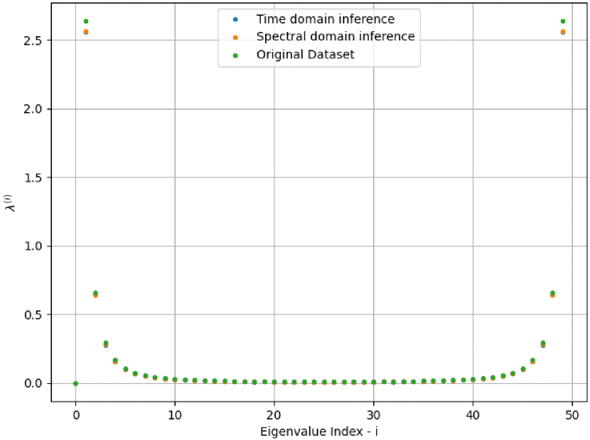
(a) A comparison of the eigenvalues obtained from each method

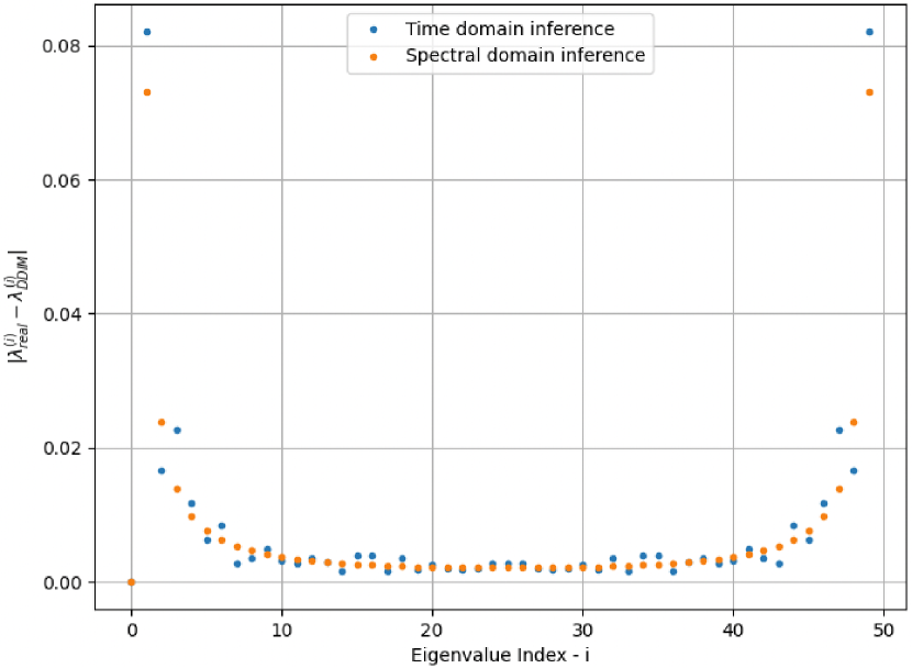
(b) The absolute relative error between the estimated eigenvalues and the data eigenvalues.

Figure 8: Figure 8(a) compares the eigenvalues derived from the spectral and time domain formulations of the DDIM method (Ho et al., 2020). The dataset, described in 6.1 with $l=0.1$ and $\text{d}=50$, is used for both approaches, involving $112$ diffusion steps and following the linear noise schedule proposed in (Song et al., 2021a). Furthermore, 8(b) illustrates the absolute error between the estimated and original eigenvalues for both methods.

Figure 8(a) shows that the derived eigenvalues from both procedures align with each other, thus verifying the transition from the time to frequency domain. However, they are not necessarily identical to the properties of the original dataset. Notably, as the number of steps increases, both processes converge toward the original dataset values. Figure 8(b) allows for an examination of the absolute error in each process relative to the characteristics of the original dataset. It is evident that while the spectral equation exhibits stable behavior, the time-domain equation displays fluctuations that depend on the number of sampled signals. As the number of samples increases, these fluctuations diminish.

G.2 Constraint Omission and Different Types of Initializations

We explore the influence of the initializations and the inequality constraints in the optimization problem. Figures 9 and 10 illustrate the evolution of the noise schedule parameter, $\{\bar{\alpha}_{s}\}_{s=0}^{S}$, during the optimization process for two different initializations: uniformly random and linearly decreasing schedules, respectively. In both cases, the diffusion process consists of $28$ steps, and the Wasserstein-2 distance is used. Each scenario was conducted twice: once with the inequality constraints from 4 and once without. The results are plotted at $15$ evenly spaced intervals throughout the process to avoid presenting each individual optimization step.

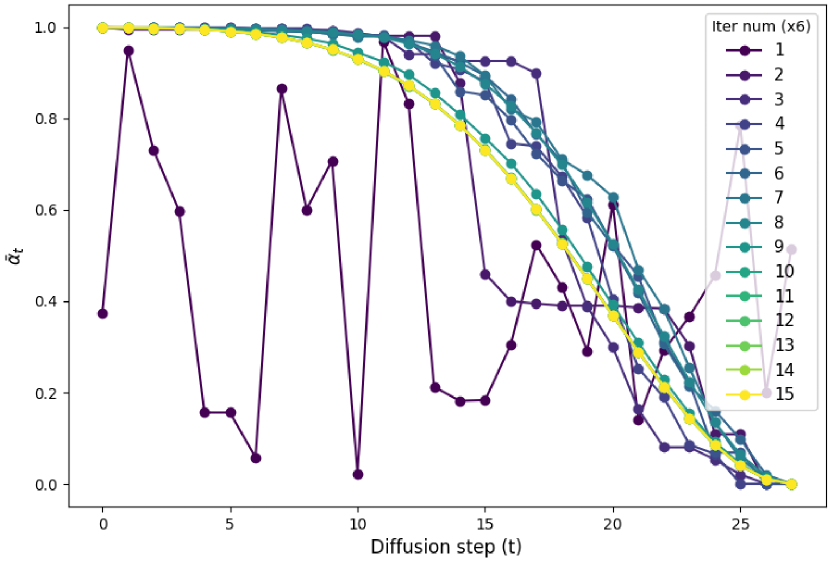
(a) Optimization with inequality constraints.

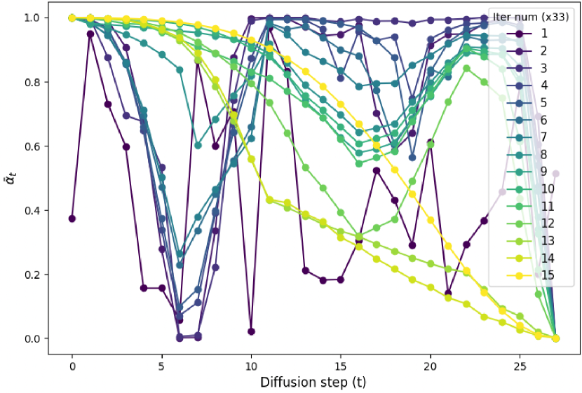
(b) Optimization without inequality constraints.

Figure 9: A Comparison of the noise schedule parameters, $\{\bar{\alpha}_{s}\}_{s=0}^{S}$, during the optimization process. The optimization was conducted over 28 diffusion steps, with a uniformly random initialization. Figure 9(a) shows the results with inequality constraints, and Figure 9(b) presents those without.

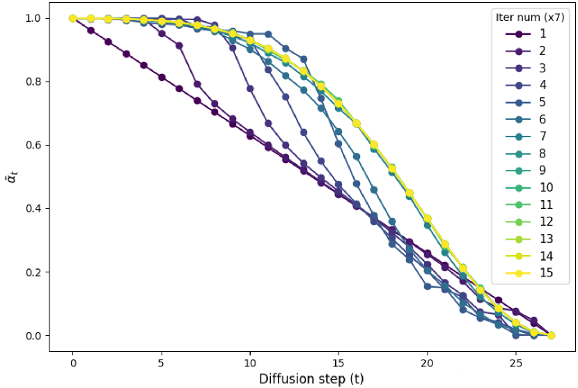
(a) Optimization with inequality constraints.

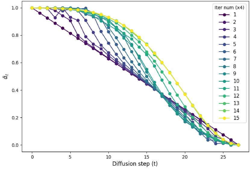
(b) Optimization without inequality constraints.

Figure 10: A Comparison of the noise schedule parameters, $\{\bar{\alpha}_{s}\}_{s=0}^{S}$, during the optimization process. The optimization was conducted over 28 diffusion steps, with a Linearly decreasing initialization. Figure 10(a) shows the results with inequality constraints, and Figure 10(b) presents those without.

The results reveal that the optimized schedule is consistent across both initializations and independent of the inequality constraints. This suggests that known characteristics of noise schedules, such as monotonicity, naturally emerge from the problem’s formulation itself, even without an explicit demand for inequality constraints. Similar consistency is observed for other initializations, including linear and cosine schedules, demonstrating the stability of the optimization procedure.

Appendix H Supplementary Experiments for Scenario 1

In the following sections, we demonstrate the received spectral recommendations for various alternative selections, applied to the matrix $\boldsymbol{\Sigma}_{0}$ and the vector $\boldsymbol{\mu}_{0}$, differing from those presented in Section 6.1. Additionally, we present the solutions obtained for defining the Wasserstein-2 distance and the KL-divergence. Through this, we aim to provide a broader perspective on the behavior and applicability of the proposed approach.

Figure 11 visualizes the covariance matrices $\boldsymbol{\Sigma}_{0}$ and $\boldsymbol{\Lambda}_{0}$ as discussed in Sec. 6.1.

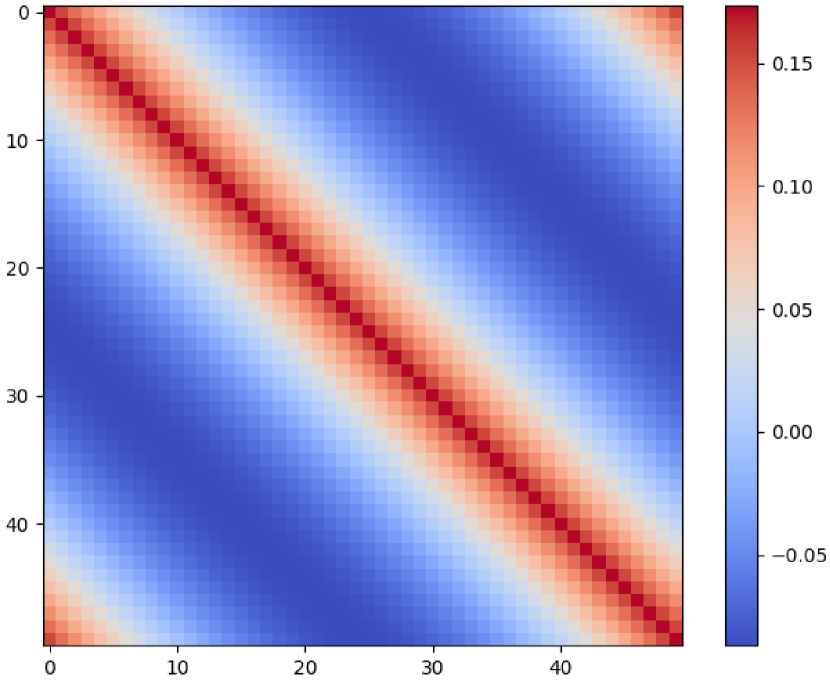
(a) $\boldsymbol{\Sigma}_{0}$

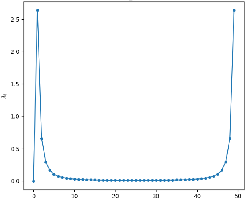
(b) $tr(\mathbf{\Lambda}_{0})$

Figure 11: Visualization of $\boldsymbol{\Sigma}_{0}$ and the trace of $\mathbf{\Lambda}_{0}$ for $d=50$ and $l=0.1$. The covariance matrix $\boldsymbol{\Sigma}_{0}$ is circulant (11(a)), while $\mathbf{\Lambda}_{0}$ is diagonal with symmetric diagonal elements (11(b)).

H.1 Wasserstein-2 distance

Figure 12 presents the resulting noise schedule based on the Wasserstein-2 distance.

(a)

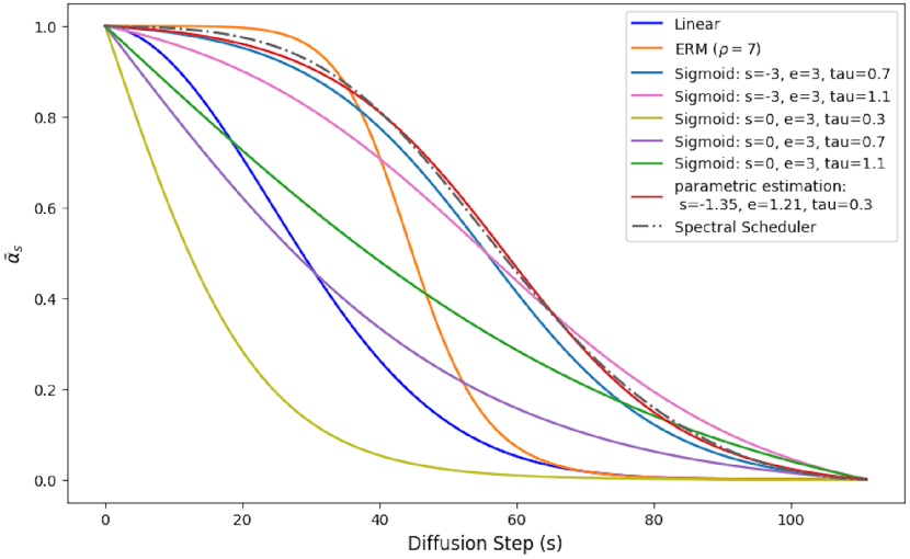
(b)

Figure 12: Figures 12(a) and 12(b) compare the optimized noise schedules from Sec. 6.1, using $d=50$, $l=0.1$, and $\boldsymbol{\mu}_{0}=0.05$, with heuristic schedules for 112 diffusion steps, where the optimization is based on the Wasserstein-2 distance. 12(a) examines the spectral schedule alongside the Linear (Ho et al., 2020), EDM (Karras et al., 2022) and Cosine-based schedules, including Cosine ($s=0$, $e=1$, $\tau=1$) from (Nichol & Dhariwal, 2021; Chen, 2023). Likewise, 12(b) compares it to Sigmoid-based schedules (Jabri et al., 2023). The parametric estimations for the Cosine and Sigmoid functions are highlighted in red.

H.2 KL-Divergence

Figure 13 presents the resulting noise schedule based on the KL-Divergence.

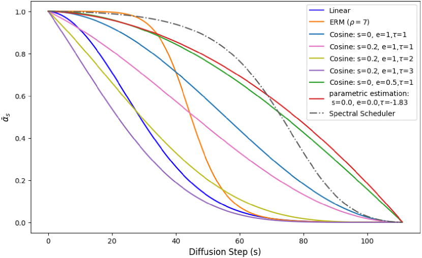
(a)

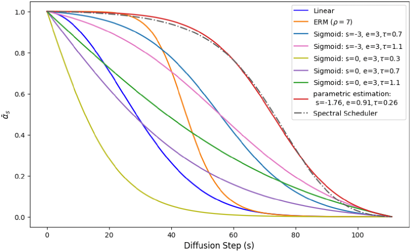
(b)

Figure 13: Figures 13(a) and 13(b) compare the optimized noise schedules from Sec. 6.1, using $d=50$, $l=0.1$, and $\boldsymbol{\mu}_{0}=0.05$, with heuristic schedules for 112 diffusion steps, where the optimization is based on the KL divergence. 13(a) examines the spectral schedule alongside the Linear (Ho et al., 2020), EDM (Karras et al., 2022) and Cosine-based schedules, including Cosine ($s=0$, $e=1$, $\tau=1$) from (Nichol & Dhariwal, 2021; Chen, 2023). Likewise, 12(b) compares it to Sigmoid-based schedules (Jabri et al., 2023). The parametric estimations for the Cosine and Sigmoid functions are highlighted in red.

Notably, under the same conditions, the KL divergence results in a more concave spectral recommendation compared to the Wasserstein-2 distance.

H.3 Variations in Covariance Matrices and Mean Configurations

In 6.1, we designed a specific covariance matrix $\boldsymbol{\Sigma}_{0}$ and a mean vector $\boldsymbol{\mu}_{0}$ with the intention of resembling characteristics observed in real signals, such as a centered signal with $\boldsymbol{\mu}_{0}\approx\mathbf{0}$. However, the optimization process is not restricted to these particular choices and can be generalized to accommodate various alternative decisions. Figure 14 displays different covariance matrices along with their corresponding $\boldsymbol{\mu}_{0}$ vectors, followed by the resulting spectral schedules computed using the Wasserstein-2 distance for $60$ diffusion steps.

(a)

(b)

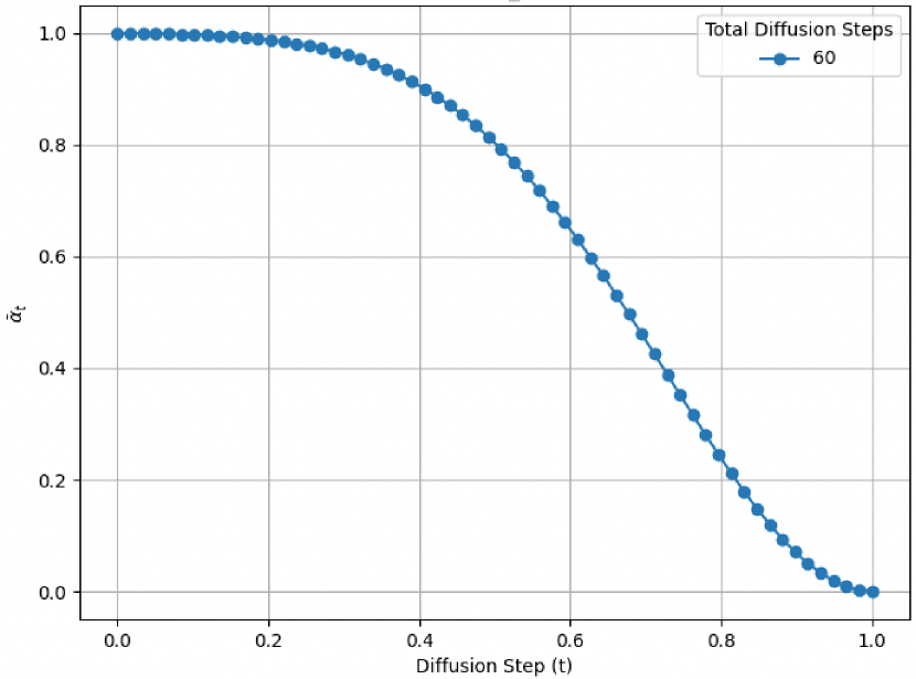
(c)

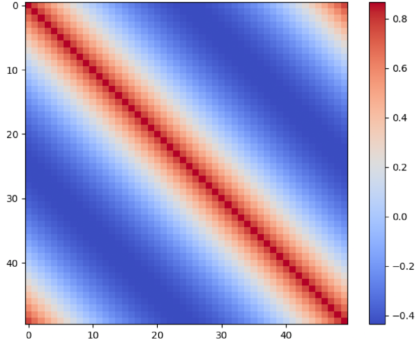
(d)

(e)

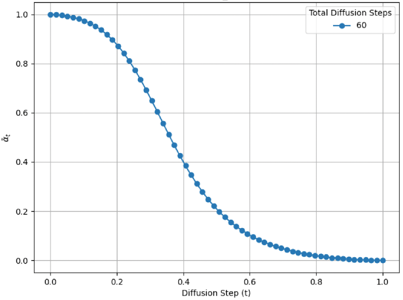
(f)

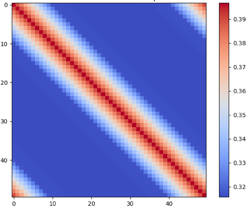
(g)

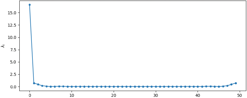
(h)

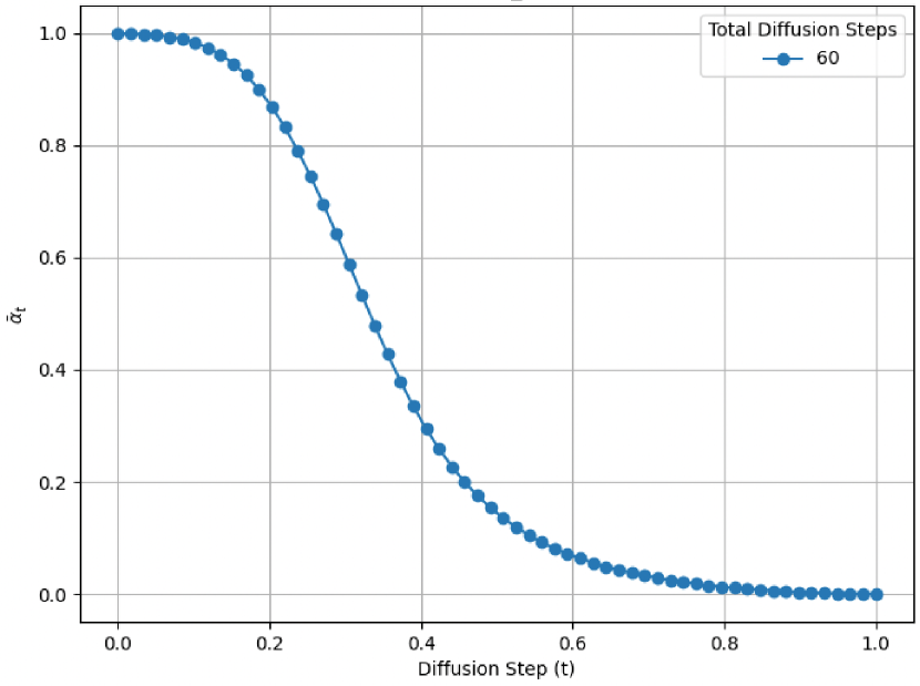
(i)

(j)

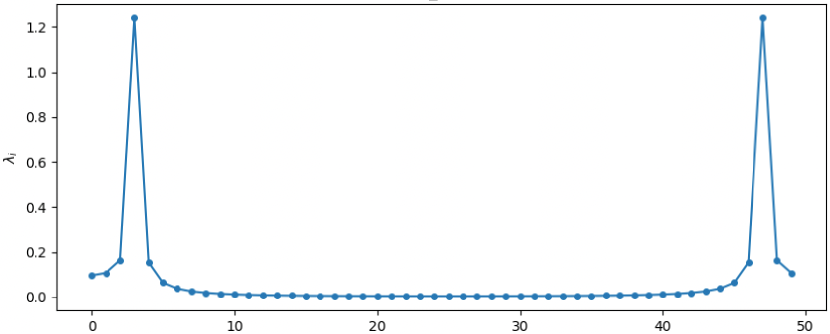
(k)

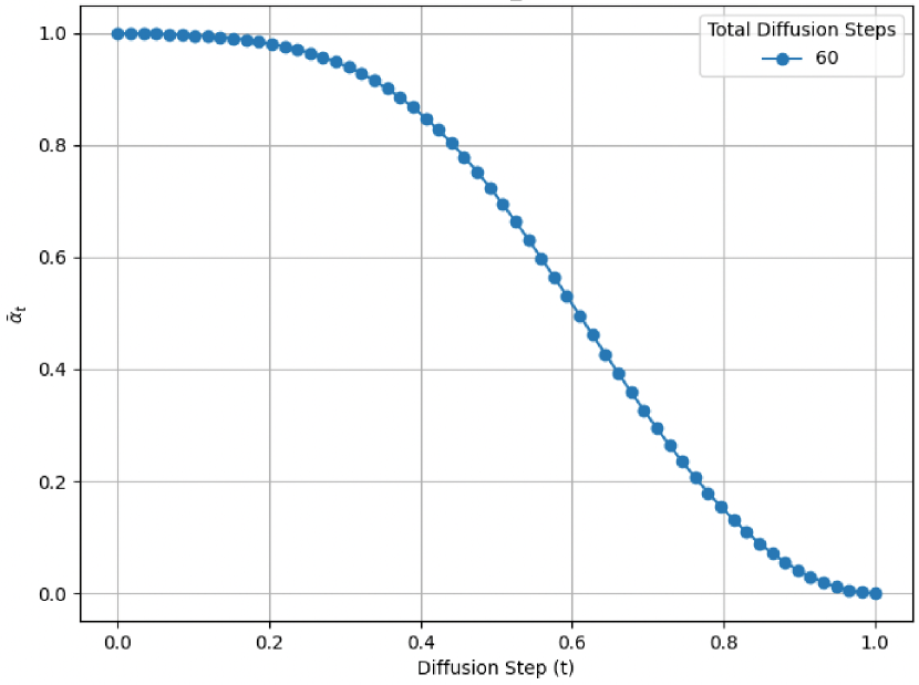
(l)

Figure 14: Various covariance matrices (first column) along with their eigenvalues (second column) and the corresponding optimized noise schedules (third column). The first row presents the matrix from 6.1 with $l=0.05$, $\boldsymbol{\mu}_{0}=0.01\cdot\mathbf{1}_{d}$. The second row shows the same matrix scaled by a factor of $20$ while keeping the same $\boldsymbol{\mu}_{0}$. The third row displays a covariance matrix incorporating a Cosine function in the first row $a$ of the circulant covariance, with $\boldsymbol{\mu}_{0}=0.3\cdot\mathbf{1}_{d}$. The fourth row features a circulant matrix derived from a sinusoidal signal with a frequency of $1000$ in the first row $a$ of the circulant covariance matrix, scaled by 0.01, and with $\boldsymbol{\mu}_{0}=0.1\cdot\mathbf{1}_{d}$.

While we cannot cover all possible choices for the covariance matrix $\boldsymbol{\Sigma}_{0}$ and the vector $\boldsymbol{\mu}_{0}$, we aim to provide a broader perspective on the KL-divergence loss. Figure 15 illustrates a circulant covariance matrix whose first row is derived from a sinusoidal signal with a frequency of $1000$ Hz, along with the corresponding spectral recommendation based on KL-divergence, where $\boldsymbol{\mu}_{0}=0.1\cdot\mathbf{1}_{d}$.

(a) $\boldsymbol{\Sigma}_{0}$

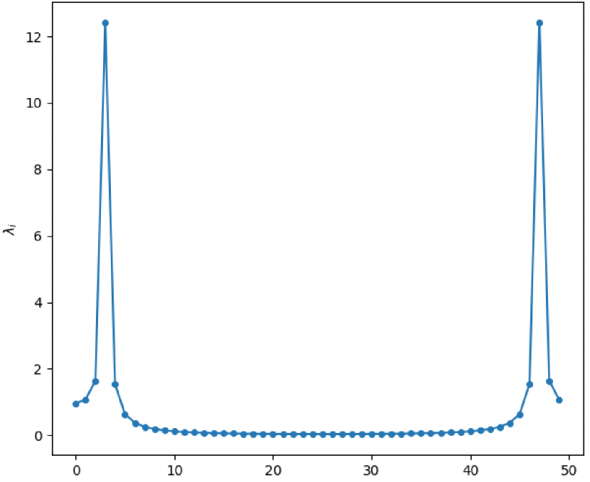
(b) $tr(\mathbf{\Lambda}_{0})$

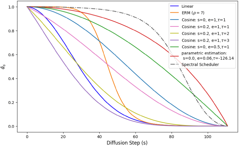
(c)

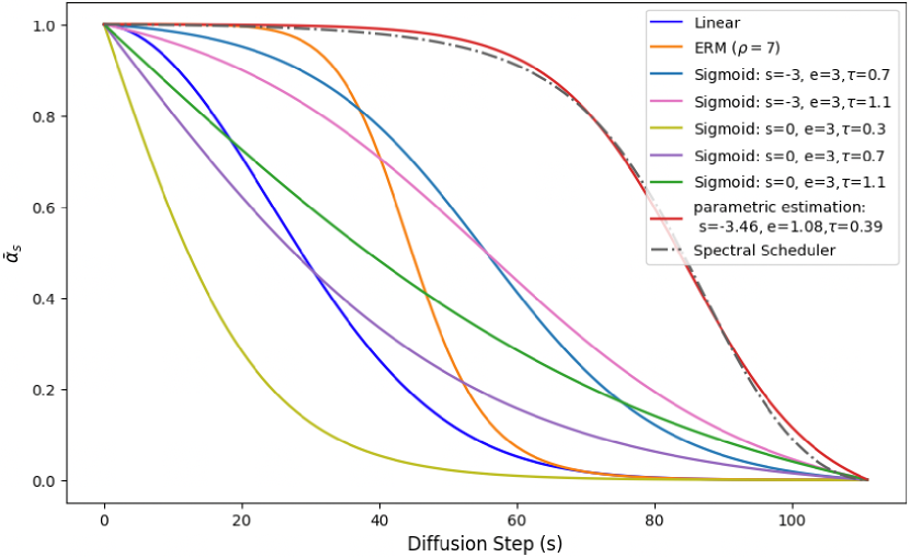
(d)

Figure 15: Figure 15(a) shows the circulant covariance matrix, $\boldsymbol{\Sigma}_{0}$, whose first row is derived from a sinusoidal signal with a frequency of $1000$ Hz. Figure 15(b) displays the trace of the corresponding $\boldsymbol{\Lambda}_{0}$ matrix. Figures 15(c) and 15(d) compare the spectral recommendations for $d=50$, $112$ diffusion steps, using the KL-divergence, with various noise schedule heuristics including Cosine and Sigmoid, respectively. The parametric estimations for the Cosine and Sigmoid are highlighted in red.

The results above show that modifying the dataset properties, such as the covariance matrix and expectation, along with altering the loss function, leads to noise schedules with a similar overall structure but varying details. In Appendix J, we explore the connection between the dataset properties, the loss function, and the resulting noise schedules.

Appendix I Supplementary Experiments for Scenario 2

We present additional details on the Gaussian MUSIC piano and SC09 datasets, along with the spectral noise schedules derived from them (Moura et al., 2020; Warden, 2018).

I.1 MUSIC Dataset

Figure 16 provides a visual representation of the estimated covariance matrix $\boldsymbol{\Sigma}_{0}$ and its corresponding $\boldsymbol{\Lambda}_{0}$, as discussed in Sec. 6.2.

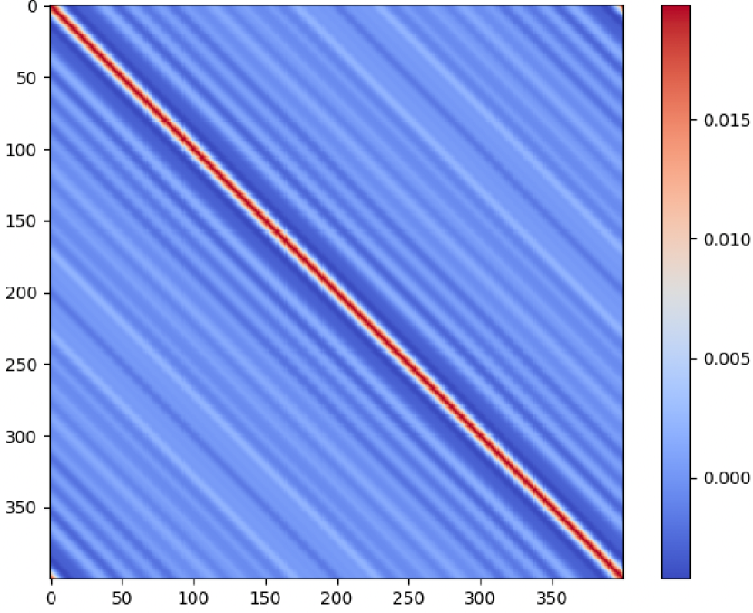
(a) $\boldsymbol{\Sigma}_{0}$

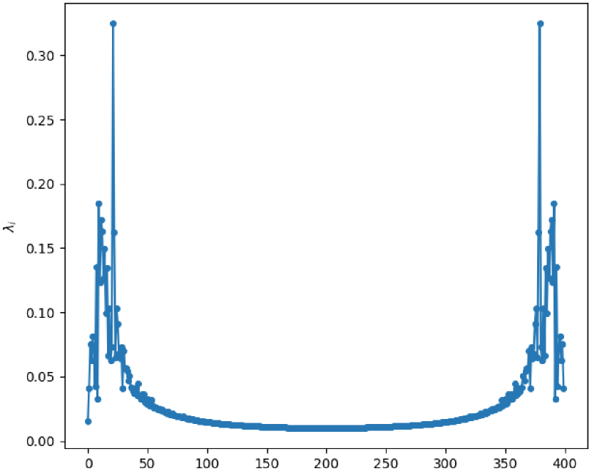
(b) $\text{tr}\left(\boldsymbol{\Lambda}_{0}\right)$

Figure 16: 16(a) illustrates $\boldsymbol{\Sigma}_{0}$, the Circulant approximation of the Covariance matrix for the MUSIC piano dataset with $d=400$ and $th=0.05$, while 16(b) displays its DFT coefficients (the eigenvalues). $\boldsymbol{\mu}_{0}\approx\boldsymbol{0}$ is also calcualted from the dataset.

I.2 SC09 Dataset

In this section, we apply our method to a different dataset, SC09. SC09 is a subset of the Speech Commands Dataset (Warden, 2018) and consists of spoken digits ($0$–$9$). Each audio sample has a duration of one second and is recorded at a sampling rate of $16$ kHz.

Differing from Sec. 6.2, here we use segments of length $d=16000$ samples (one second) and set $th=0.05$ in one setting and $0.1$ in another. Figure 17 presents the spectral recommendations for $th=0.05$ and $th=0.1$ in the left and right columns, respectively.

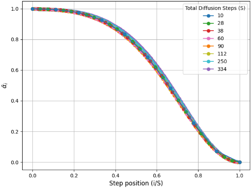
(a)

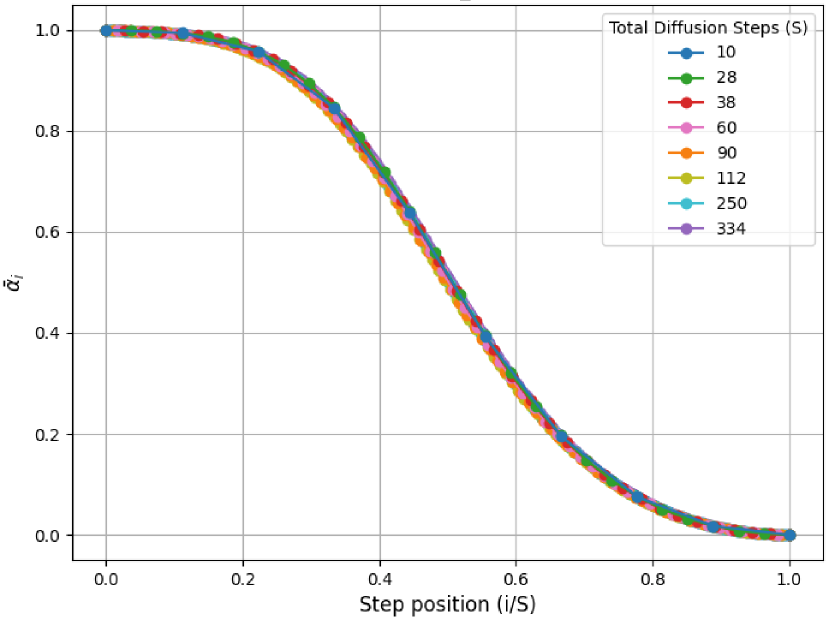
(b)

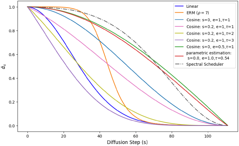
(c)

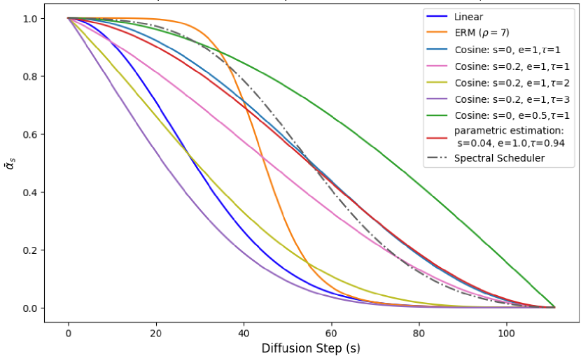
(d)

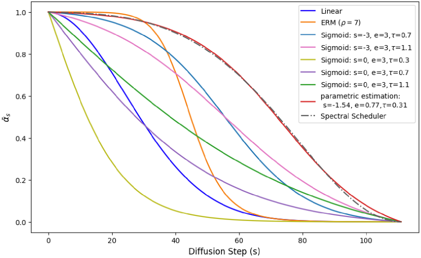
(e)

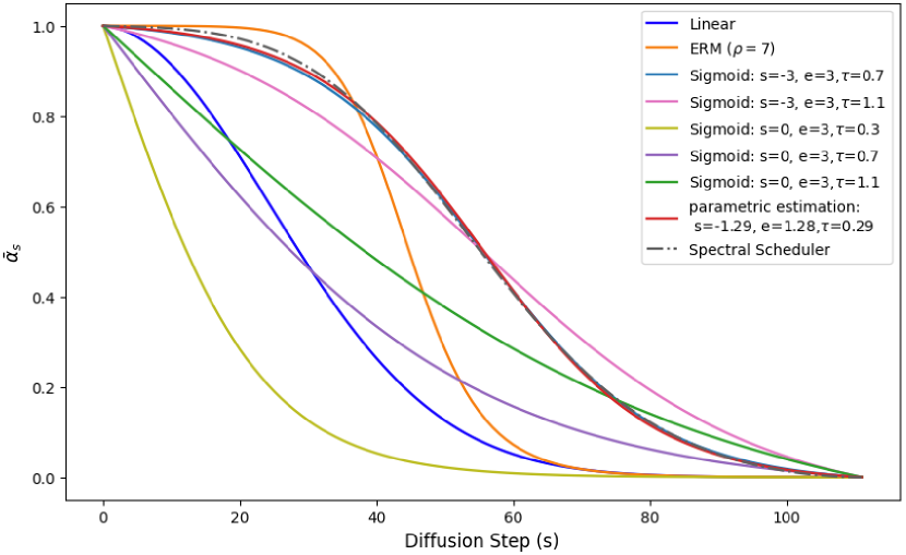
(f)

Figure 17: Spectral noise schedules for the $SC09$ dataset with $d=16,000$ and thresholds $th=0.05$ (left column) and $th=0.1$ (right column). The first row shows spectral recommendations for various diffusion steps, while the second and third rows compare the spectral recommendation for $112$ steps with heuristic noise schedules, including the Cosine and Sigmoid schedules. The parametric estimations for the Cosine and Sigmoid functions are shown in red, respectively.

Figures 17(a) and 17(b) demonstrate that the spectral recommendation for $th=0.05$ exhibits a more concave behavior compared to $th=0.1$. A more detailed discussion on the influence of the $th$ and $d$ parameters on the covariance matrix and the resulting noise schedule is provided in Appendices I.3 and J.

I.3 Analysis of Different Aspects

The estimation of the covariance matrix, which is essential for finding the spectral recommendation for a real dataset, relies on the choice of two key parameters: $th$ and $d$.

The parameter $d$ represents the dimension of the signals and controls the frequency resolution, which affects the eigenvalues. A smaller $d$ may result in a more generalized eigenvalue spectrum, reducing accuracy by averaging energy across neighboring eigenvalues. In contrast, a larger $d$ improves the precision in capturing frequency details but increases computational time for both estimation and optimization.

Figure 18 shows that as $d$ increases, the eigenvalue structure becomes more precise, with the maximum eigenvalues magnitude growing larger. Conversely, as $d$ decreases, the eigenvalue structure becomes more generalized, exhibiting a monotonic decrease, as discussed in Appendix J.2.

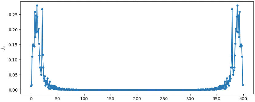
(a) $d=400$

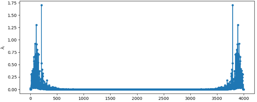
(b) $d=4000$

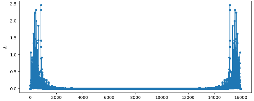
(c) $d=16000$

Figure 18: Eigenvalues of the MUSIC dataset using $d=[400,4000,16000]$

An additional consideration is the choice of the threshold value $th$. This threshold helps prevent the covariance matrix estimation from being overly influenced by silent regions in the signal, which are characterized by low $L_{1}$ energy. Adjusting $th$ affects both the covariance matrix values and the eigenvalues, i.e. $C\cdot Av=C\cdot\lambda v$, thereby influencing the resulting noise schedule, as shown in Appendix J.1.

Appendix J Further Discussion

J.1 Relationship Between Noise Schedules and Eigenvalues

To explore the relationship between the optimal spectral noise schedule and the dataset characteristics, we solved the optimization problem for each eigenvalue individually, with the contributions from the other eigenvalues set to zero. Using the eigenvalues of the covariance matrix from 6.1, Figure 19(a) shows these eigenvalues, while 19(b) presents the optimal solutions for $50$ diffusion steps, computed using the Wasserstein-2 distance in the optimization problem. Each solution corresponds to a single eigenvalue (considering only positions $2$ to $10$ for clarity)

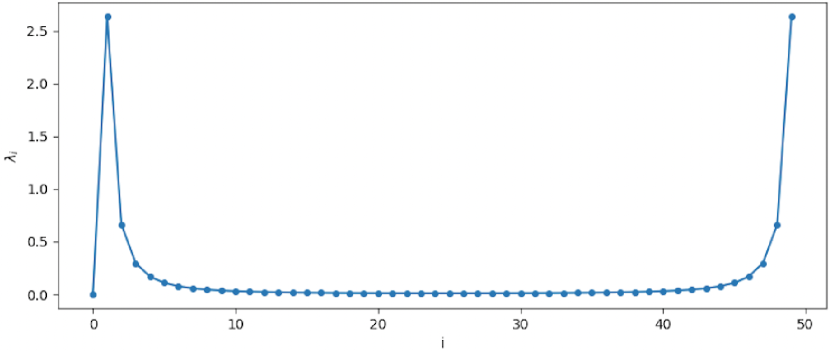
(a)

(b)

Figure 19: Figure 19(a) shows the eigenvalues for the covariance matrix from Section 6.1. Figure 19(b) presents the results of solving the optimization problem for each eigenvalue individually, with the contributions from the other eigenvalues set to zero.

It can be observed from Figure 19(b) that the solution becomes more concave as the magnitude of the eigenvalue decreases (yellow) and more convex as the magnitude increases (blue). Notably, this behavior is determined by the magnitude of the eigenvalues ($\{\lambda_{i}\}_{i=1}^{d}$) rather than their indices ($i$), as the objective functions are independent of the index itself.

Interestingly, by examining the spectral recommendation from Figure 1, it closely resembles the solutions obtained by emphasizing the highest eigenvalue (19(b)). This suggests that using the Wasserstein-2 loss tends to favor larger magnitude eigenvalues. This behavior is also reflected in the relative error, $(|\lambda_{i}-\lambda_{est}|)/(\lambda_{i})$, shown in Figure 20, where larger eigenvalues exhibit smaller relative errors.

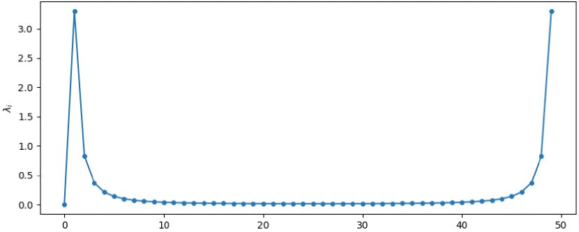
(a)

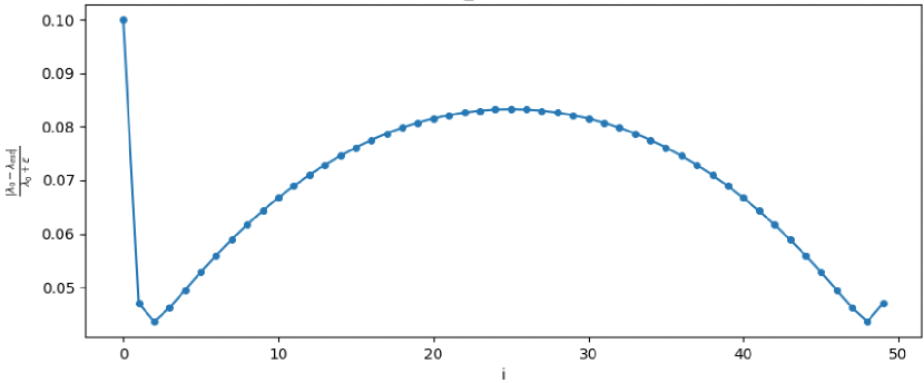
(b)

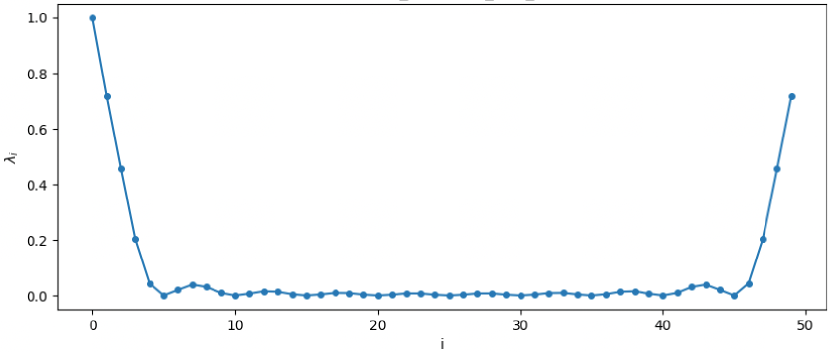
(c)

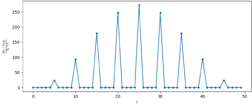
(d)

Figure 20: Figures 20(a) and 20(c) present the eigenvalues of matrices 14(a) and 14(g), respectively. Figures 20(b) and 20(d) illustrate the relative error of the spectral recommendation, using $60$ diffusion steps and the Wasserstein-2 distance. Notably, larger eigenvalues exhibit smaller relative errors. In Figures 20(b) and 20(c), the first elements were manually chosen, as they originally had extreme values ($1000$ and $10$ respectively), and we aimed to keep the figure within a reasonable scale.

The influence of the eigenvalue magnitude, particularly that of the dominant eigenvalues, on the resulting schedule is further illustrated through additional examples. Figure 14(d) displays the covariance matrix from Figure 14(a), scaled by a factor of $C=20$, which amplifies the dominant eigenvalues, as shown by the relation $C\cdot Av=C\cdot\lambda v$. Consequently, the spectral recommendation in Figure 14(f) appears more convex than in Figure 14(c). A similar trend is observed in Figure 17, where the spectral recommendation for $th=0.05$ exhibits a more concave shape compared to $th=0.1$.

This relationship open up a possibility of designing loss functions which focus on specific frequency ranges of interest. When the eigenvalues, or equivalently the DFT coefficients, decrease monotonically, a direct relationship emerges between the eigenvalue magnitude and its corresponding frequency (for example, the $1/f$ behavior observed in speech (Voss & Clarke, 1975)). Further discussion is provided in J.2.

Note: We used the Wasserstein-2 loss. However, alternative measures, such as KL divergence ,could also yield similar results.

J.2 Relationship Between Noise Schedules and the loss functions

As mentioned in 3.3, assuming circularity, the eigenvalues correspond to the DFT coefficients of first row of $\boldsymbol{\Sigma}_{0}$. When the eigenvalues, or equivalently the coefficients of the Discrete Fourier Transform, decrease monotonically, there is a direct relationship between the magnitude of the eigenvalue and its corresponding frequency (for example, $1/f$ behavior observed in speech (Voss & Clarke, 1975)). In such cases, the first eigenvalues correspond to the low frequencies, having larger amplitudes, while the last correspond to high frequencies and smaller amplitudes. This pattern, along, with the observations in Appendix J, aligns with the well-known coarse-to-fine signal construction behavior of diffusion models. Building on this monotonicity behavior, the loss function can be adjusted to weight different frequency regions in various ways, shaping the noise schedule based on specific objectives.

We propose a weighted l1 loss for the first and the second moments of two Gaussian distributions $P(\mathbf{\hat{x}_{0}^{\mathcal{F}}};\bar{\boldsymbol{\alpha}})$ and $P(\mathbf{{x}_{0}^{\mathcal{F}}})$.

$$\mathcal{D}_{L_{1}}\big{(}P(\mathbf{\hat{x}_{0}^{\mathcal{F}}};\bar{\boldsymbol{\alpha}}),P(\mathbf{{x}_{0}^{\mathcal{F}})}\big{)}=\sum_{i=1}^{d}\frac{\mathbf{\lambda}_{i}}{\sum_{j}\mathbf{\lambda}_{j}}\left|[\mathbf{D}_{1}]_{i}^{2}-\mathbf{\lambda}_{i}\right|+\sum_{i=1}^{d}\frac{[\boldsymbol{\mu}_{0}^{\mathcal{F}}]^{2}_{i}}{\sum_{j}[\boldsymbol{\mu}_{0}^{\mathcal{F}}]^{2}_{j}}\left([\mathbf{D}_{2}]_{i}-1\right)^{2}$$ (62)

The first term applies a weighted l1 loss to the eigenvalues, while the second term computes a weighted l2 norm of the mean vectors. This design ensures that eigenvalues with larger magnitudes and mean components with higher values have greater influence on the overall loss.

Figure 21 illustrates the spectral recommendation obtained by solving the optimization problem in 15 using the Weighted l1 loss. The results are based on the Gaussian MUSIC-Piano dataset described in 6.2 where $d=16,000$ and $th=0.05$.

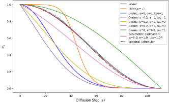
Figure 21: Comparison of the spectral schedule with various heuristic noise schedules for $S=112$ diffusion steps. The figure presents the linear, EDM ($\rho=7$), Cosine-based schedules, including Cosine ($s=0$, $e=1$, $\tau=1$) from (Nichol & Dhariwal, 2021; Chen, 2023). The parametric estimation of the cosine function is shown in red.

Interestingly, using the weighted l1 loss results in a spectral recommendation that aligns with established heuristic methods. Specifically, it corresponds to the manually designed cosine (0,1,1) schedule proposed in (Nichol & Dhariwal, 2021). This observation could indicate a potential link between the design of widely used noise schedule heuristics and a bias against high-frequency generation, which has been observed in previous research (Yang et al., 2023).

Note: The relationship between the magnitude of the eigenvalues and their corresponding frequencies holds tight only when monotonic behavior is present. In real-world scenarios, as shown in Figure 18(c), the eigenvalues’ magnitudes generally decrease, but the function is not strictly monotonic. In such cases, an alternative approach is required, one that either analyzes broader frequency regions or considers both the values and indices of the eigenvalues.

Appendix K Analysis of Mean Bias

We analyze the mean bias expression $(\mathbf{D}_{2}-\mathbf{I})\boldsymbol{\mu_{0}^{\mathcal{F}}}$ , which arises from the difference between $\mathbb{E}\left[\mathbf{\mathbf{x}}_{0}^{\mathcal{F}}\right]$ and $\mathbb{E}\left[\mathbf{\hat{\mathbf{x}}}_{0}^{\mathcal{F}}\right]$. In particular, We will focus on the absolute magnitude of the expression $|\mathbf{D}_{2}-\mathbf{I}||\boldsymbol{\mu_{0}^{\mathcal{F}}}|$. The term $\mathbf{D}_{2}$, as defined in (11), depends on $\boldsymbol{\Lambda}_{0}$ and on $\bar{\boldsymbol{\alpha}}$, the chosen noise schedule. Notably, for stationary signals, $\boldsymbol{\mu}_{0}$ is deterministic, resulting in the vector $\boldsymbol{\mu_{0}^{\mathcal{F}}}$ where all entries are zero except for the first element. specifically, for a mean-centered signal where $\boldsymbol{\mu_{0}^{\mathcal{F}}}=\boldsymbol{0}$, the DDIM process remains unbiased, regardless of $|\mathbf{D}_{2}-\mathbf{I}|$ expression. In other cases, for a given $\boldsymbol{\mu_{0}^{\mathcal{F}}}$, the primary source of bias originates from the main diagonal of $|\mathbf{D}_{2}-\mathbf{I}|$.

Figure 22 analyzes the mean bias for two choices of $\boldsymbol{\Lambda}_{0}$ with $d=50$. It compares the values of $|\mathbf{D}_{2}-\mathbf{I}|$ across several cosine noise schedule heuristics and illustrates how its behavior depends on the number of diffusion steps.

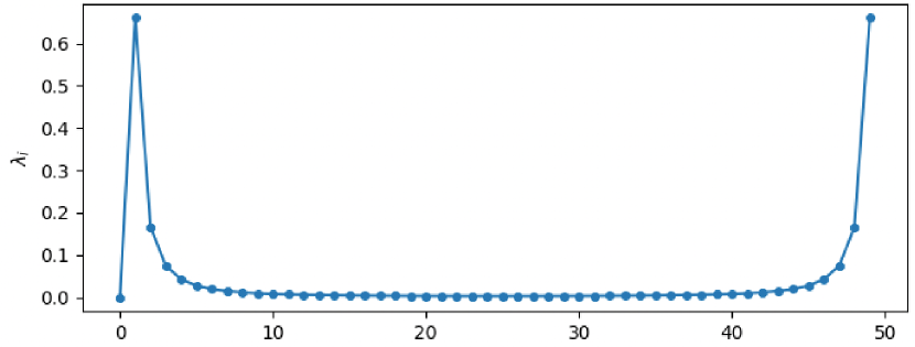
(a)

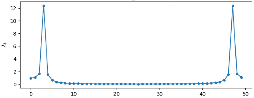
(b)

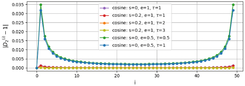
(c)

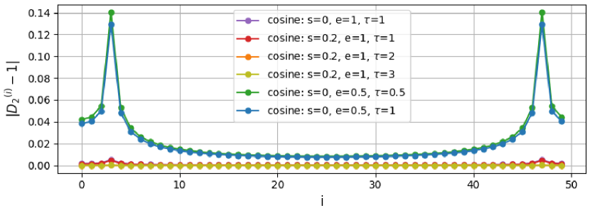
(d)

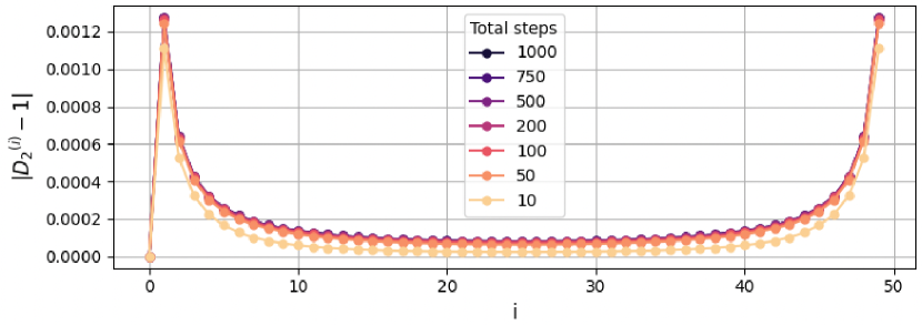
(e)

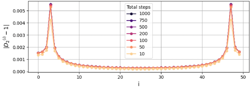
(f)

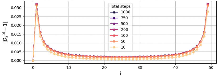
(g)

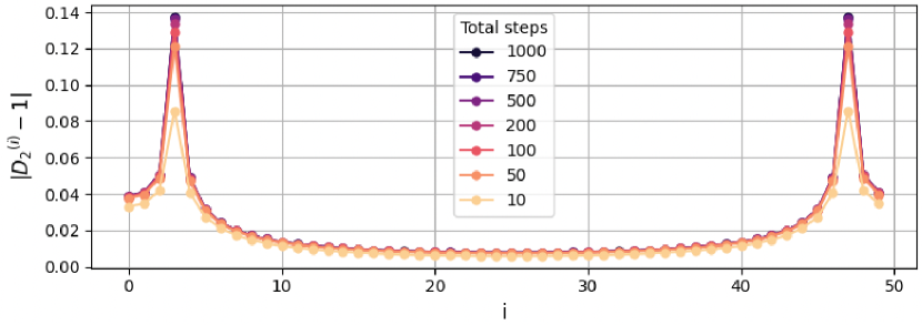
(h)

Figure 22: Figures 22(a) and 22(b) display the eigenvalues for two choices of $\boldsymbol{\Lambda}_{0}$ with $d=50$. Figures 22(c) and 22(d) compare the mean bias values across different parametrization of the Cosine noise schedule using $112$ diffusion steps. Figures 22(e) and 22(f) show the bias for varying numbers of diffusion steps with the Cosine ($0$,$1$,$1$) noise schedule, while Figures 22(g) and 22(h) illustrate the same for the Cosine ($0$,$0.5$,$1$) schedule.

Figures 22(c) and 22(d) reveal that for certain heuristics, such as Cosine ($0$,$1$,$1$), the bias is negligible, while for others, like Cosine ($0$,$0.5$,$1$), the bias increases. Additionally, the magnitude of the eigenvalues $\{{\lambda}_{i}\}_{i=1}^{d}$ plays a significant role in determining the bias; as the eigenvalues grow larger, the bias also tends to increase.

Figures 22(e) and 22(f) illustrate the bias across various numbers of diffusion steps $\{10,50,100,200,500,750,1000\}$ for the Cosine ($0$,$1$,$1$) noise schedule. Similarly, Figures 22(g) and 22(h) show the bias for the Cosine ($0$,$0.5$,$1$). In both cases, increasing the number of diffusion steps leads to a gradual rise in the mean bias $|\mathbf{D}_{2}-\mathbf{I}|$.

Appendix L DDPM vs DDIM

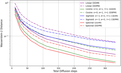
Figure 23: Comparison of the Wasserstein-2 distance between DDIM and DDPM for different noise schedules, including the spectral recommendation, across various diffusion steps.

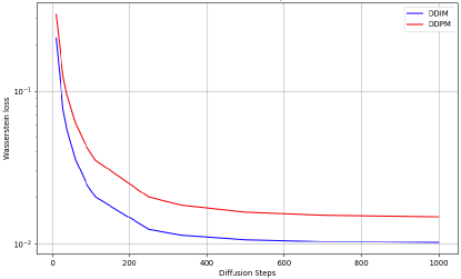
Figure 24: Comparison of the spectral noise schedules in DDPM and DDIM, derived from the covariance matrix outlined in Sec. 6.1, with parameters d=50, l=0.1, and total diffusion steps set to $\{10,28,38,60,90,112,250,334,500,750,1000\}$.

Appendix M Estimating a circulant matrix

Given a symmetric Toeplitz matrix B we aim to estimate a circulant matrix A that balances closely approximating the original matrix while preserving circulant properties. Since both symmetric Toeplitz and circulant matrices are fully characterized by their first rows, the optimization is formulated in terms of ${\left\{{X_{A}[k]}\right\}_{k=0}^{n-1}}$ and ${\left\{{X_{B}[k]}\right\}_{k=0}^{n-1}}$, which represent the first rows of A and B, respectively:

$$\arg\min_{\left\{{X_{A}[k]}\right\}_{k=0}^{n-1}}\left(X_{A}[k]-X_{B}[k]\right)^{2}\left(n-k\right)+\left(X_{A}[k]-X_{B}[N-k]\right)^{2}\left(k\right)$$

By differentiating the objective with respect to each element of ${X_{A}[k]}_{k=0}^{n-1}$ and setting the result equal to zero, we obtain:

$${X_{A}[k]}=\frac{X_{B}[k]\left(n-k\right)+X_{B}[n-k]k}{\left(n-k\right)+k},\quad\text{for }k=0,\dots,d-1$$

This approach leverages the structural properties of both matrices, ensuring that the estimated circulant matrix A remains as close as possible to B while preserving a circulant nature.

References

• Benita et al. (2024) Benita, R., Elad, M., and Keshet, J. DiffAR: Denoising diffusion autoregressive model for raw speech waveform generation. In The 12th International Conference on Learning Representations (ICLR), 2024.
• Biroli et al. (2024) Biroli, G., Bonnaire, T., De Bortoli, V., and Mézard, M. Dynamical regimes of diffusion models. Nature Communications, 15(1):9957, 2024.
• Chen et al. (2024) Chen, D., Zhou, Z., Wang, C., Shen, C., and Lyu, S. On the trajectory regularity of ODE-based diffusion sampling. In Proceedings of the 41st International Conference on Machine Learning (ICML), 2024.
• Chen et al. (2023) Chen, S., Chewi, S., Li, J., Li, Y., Salim, A., and Zhang, A. Sampling is as easy as learning the score: theory for diffusion models with minimal data assumptions. In The 11th International Conference on Learning Representations (ICLR), 2023.
• Chen (2023) Chen, T. On the importance of noise scheduling for diffusion models. arXiv preprint arXiv:2301.10972, 2023.
• Corvi et al. (2023) Corvi, R., Cozzolino, D., Poggi, G., Nagano, K., and Verdoliva, L. Intriguing properties of synthetic images: from generative adversarial networks to diffusion models. In Proceedings of the IEEE/CVF Conference on Computer Vision and Pattern Recognition, pp.  973–982, 2023.
• Davis (1970) Davis, P. J. Circulant Matrices. Wiley, New York, 1970. ISBN 0-471-05771-1.
• Ho et al. (2020) Ho, J., Jain, A., and Abbeel, P. Denoising diffusion probabilistic models. Advances in neural information processing systems, 33:6840–6851, 2020.
• Jabri et al. (2023) Jabri, A., Fleet, D. J., and Chen, T. Scalable adaptive computation for iterative generation. In Proceedings of the 40th International Conference on Machine Learning (ICML), 2023.
• Jolicoeur-Martineau et al. (2021) Jolicoeur-Martineau, A., Li, K., Piché-Taillefer, R., Kachman, T., and Mitliagkas, I. Gotta go fast when generating data with score-based models. arXiv preprint arXiv:2105.14080, 2021.
• Karras et al. (2022) Karras, T., Aittala, M., Aila, T., and Laine, S. Elucidating the design space of diffusion-based generative models. Advances in neural information processing systems, 35:26565–26577, 2022.
• Kawar et al. (2022) Kawar, B., Elad, M., Ermon, S., and Song, J. Denoising diffusion restoration models. Advances in Neural Information Processing Systems, 35:23593–23606, 2022.
• Kong et al. (2021) Kong, Z., Ping, W., Huang, J., Zhao, K., and Catanzaro, B. DiffWave: a versatile diffusion model for audio synthesis. In International Conference on Learning Representations (ICLR), 2021.
• Kraft (1988) Kraft, D. A software package for sequential quadratic programming. Forschungsbericht- Deutsche Forschungs- und Versuchsanstalt fur Luft- und Raumfahrt, 1988.
• Lin et al. (2024) Lin, S., Liu, B., Li, J., and Yang, X. Common diffusion noise schedules and sample steps are flawed. In Proceedings of the IEEE/CVF winter conference on applications of computer vision, pp.  5404–5411, 2024.
• Liu et al. (2022) Liu, L., Ren, Y., Lin, Z., and Zhao, Z. Pseudo numerical methods for diffusion models on manifolds. In International Conference on Learning Representations (ICLR), 2022.
• Lu et al. (2022) Lu, C., Zhou, Y., Bao, F., Chen, J., Li, C., and Zhu, J. Dpm-solver: A fast ode solver for diffusion probabilistic model sampling in around 10 steps. Advances in Neural Information Processing Systems, 35:5775–5787, 2022.
• Moura et al. (2020) Moura, L., Fontelles, E., Sampaio, V., and França, M. Music dataset: Lyrics and metadata from 1950 to 2019, 2020. URL https://doi.org/10.17632/3t9vbwxgr5.3.
• Nichol & Dhariwal (2021) Nichol, A. Q. and Dhariwal, P. Improved denoising diffusion probabilistic models. In International conference on machine learning (ICML), pp.  8162–8171, 2021.
• Pierret & Galerne (2024) Pierret, E. and Galerne, B. Diffusion models for gaussian distributions: Exact solutions and wasserstein errors. arXiv preprint arXiv:2405.14250, 2024.
• Rissanen et al. (2023) Rissanen, S., Heinonen, M., and Solin, A. Generative modelling with inverse heat dissipation. In The 11th International Conference on Learning Representations (ICLR), 2023.
• Sabour et al. (2024) Sabour, A., Fidler, S., and Kreis, K. Align your steps: optimizing sampling schedules in diffusion models. In Proceedings of the 41st International Conference on Machine Learning, 2024.
• Song et al. (2021a) Song, J., Meng, C., and Ermon, S. Denoising diffusion implicit models. In International Conference on Learning Representations (ICLR), 2021a.
• Song et al. (2021b) Song, Y., Sohl-Dickstein, J., Kingma, D. P., Kumar, A., Ermon, S., and Poole, B. Score-based generative modeling through stochastic differential equations. In International Conference on Learning Representations, 2021b.
• Tong et al. (2024) Tong, V., Hoang, T.-D., Liu, A., Broeck, G. V. d., and Niepert, M. Learning to discretize denoising diffusion odes. arXiv preprint arXiv:2405.15506, 2024.
• Voss & Clarke (1975) Voss, R. P. and Clarke, J. “I/F Noise” in Music and Speech. Lawrence Berkeley National Laboratory, 1975.
• Wang et al. (2023) Wang, Y., Wang, X., Dinh, A.-D., Du, B., and Xu, C. Learning to schedule in diffusion probabilistic models. In Proceedings of the 29th ACM Conference on Knowledge Discovery and Data Mining (SIGKDD), pp.  2478–2488, 2023.
• Warden (2018) Warden, P. Speech commands: A dataset for limited-vocabulary speech recognition. arXiv preprint arXiv:1804.03209, 2018.
• Watson et al. (2022) Watson, D., Chan, W., Ho, J., and Norouzi, M. Learning fast samplers for diffusion models by differentiating through sample quality. In International Conference on Learning Representations (ICLR), 2022.
• Wiener (1949) Wiener, N. Extrapolation, Interpolation, and Smoothing of Stationary Time Series. MIT Press, Cambridge, MA, 1949.
• Williams et al. (2024) Williams, C., Campbell, A., Doucet, A., and Syed, S. Score-optimal diffusion schedules. In The Thirty-eighth Annual Conference on Neural Information Processing Systems, 2024.
• Xia et al. (2024) Xia, M., Shen, Y., Lei, C., Zhou, Y., Yi, R., Zhao, D., Wang, W., and Liu, Y.-j. Towards more accurate diffusion model acceleration with a timestep aligner. In Proceedings of the IEEE/CVF Conference on Computer Vision and Pattern Recognition (CVPR), 2024.
• Xue et al. (2024) Xue, S., Liu, Z., Chen, F., Zhang, S., Hu, T., Xie, E., and Li, Z. Accelerating diffusion sampling with optimized time steps. In Proceedings of the IEEE/CVF Conference on Computer Vision and Pattern Recognition, pp.  8292–8301, 2024.
• Yang et al. (2023) Yang, X., Zhou, D., Feng, J., and Wang, X. Diffusion probabilistic model made slim. In Proceedings of the IEEE/CVF Conference on Computer Vision and Pattern Recognition, pp.  22552–22562, 2023.
• Zhang & Chen (2023) Zhang, Q. and Chen, Y. Fast sampling of diffusion models with exponential integrator. In The Eleventh International Conference on Learning Representations, 2023.
• Zhao et al. (2024) Zhao, W., Bai, L., Rao, Y., Zhou, J., and Lu, J. Unipc: A unified predictor-corrector framework for fast sampling of diffusion models. Advances in Neural Information Processing Systems, 36, 2024.
• Zheng et al. (2023) Zheng, K., Lu, C., Chen, J., and Zhu, J. Dpm-solver-v3: Improved diffusion ode solver with empirical model statistics. Advances in Neural Information Processing Systems, 36:55502–55542, 2023.