Offline Learning for Combinatorial Multi-armed Bandits

Abstract

The combinatorial multi-armed bandit (CMAB) is a fundamental sequential decision-making framework, extensively studied over the past decade. However, existing work primarily focuses on the online setting, overlooking the substantial costs of online interactions and the readily available offline datasets. To overcome these limitations, we introduce Off-CMAB, the first offline learning framework for CMAB. Central to our framework is the combinatorial lower confidence bound (CLCB) algorithm, which combines pessimistic reward estimations with combinatorial solvers. To characterize the quality of offline datasets, we propose two novel data coverage conditions and prove that, under these conditions, CLCB achieves a near-optimal suboptimality gap, matching the theoretical lower bound up to a logarithmic factor. We validate Off-CMAB through practical applications, including learning to rank, large language model (LLM) caching, and social influence maximization, showing its ability to handle nonlinear reward functions, general feedback models, and out-of-distribution action samples that excludes optimal or even feasible actions. Extensive experiments on synthetic and real-world datasets further highlight the superior performance of CLCB.

1 Introduction

Combinatorial multi-armed bandit (CMAB) is a fundamental sequential decision-making framework, designed to tackle challenges in combinatorial action spaces. Over the past decade, CMAB has been extensively studied [1, 2, 3, 4, 5, 6, 7, 8, 9, 10, 11, 12, 13, 14, 15, 16, 17], driving advancements in real-world applications like recommendation systems [18, 19, 20, 21], healthcare [22, 23, 24], and cyber-physical systems [25, 26, 27, 28] .

Most success stories of CMAB have emerged within the realm of online CMAB [5, 6, 7, 8, 9, 10, 11, 21, 29, 13], which relies on active data collection through online exploration. While effective in certain scenarios, this framework faces two major limitations. On one hand, online exploration becomes impractical when it incurs prohibitive costs or raises ethical and safety concerns. On the other hand, they neglect offline datasets that are often readily available at little or no cost. For instance, in healthcare systems [30], recommending optimal combinations of medical treatments—such as drugs, surgical procedures, and radiation therapy—requires extreme caution. Experimenting directly on patients is ethically and practically infeasible. Instead, leveraging pre-collected datasets of prior treatments can help to make informed decisions while ensuring patient safety. Similar happens for recommendation systems [31] and autonomous driving [32], offline datasets such as user click histories and human driving logs are ubiquitous. Leveraging these offline datasets can guide learning agents to identify optimal policies while avoiding the significant costs associated with online exploration—such as degrading user experience or risking car accidents.

To address the limitations of online CMAB, we propose the first offline learning framework for CMAB (Off-CMAB), where we leverage a pre-collected dataset consisting of $n$ samples of combinatorial actions and their corresponding feedback data. Our framework handles rewards that are nonlinear functions of the chosen super arms and considers general probabilistic feedback models, supporting a wide range of applications such as learning to rank [33], large language model (LLM) caching [34], and influence maximization [35]. The objective is to identify a combinatorial action that minimizes the suboptimal gap, defined as the reward difference between the optimal action and the identified action. The key challenge of Off-CMAB lies in the absence of access to an online environment, which inherently limits the number of data samples available for each action. Furthermore, this problem becomes even more challenging with the combinatorially large action space, which complicates the search for optimal solutions, and the potential presence of out-of-distribution (OOD) samples, where the dataset may exclude optimal or even feasible actions. To tackle these challenges, this work makes progress in answering the following two open questions:

(1) Can we design a sample-efficient algorithm for Off-CMAB when the action space is combinatorially large? (2) How much data is necessary to find a near-optimal action, given varying levels of dataset quality?

We answer these questions from the following perspectives:

Algorithm Design: To address the first question, we propose a novel combinatorial lower confidence bound (CLCB) algorithm that addresses the uncertainty inherent in passively collected datasets by leveraging the pessimism principle. At the base arm level, CLCB constructs high-probability lower confidence bounds (LCBs), penalizing arms with insufficient observations. At the combinatorial action level, CLCB utilizes an approximate combinatorial solver to handle nonlinear reward functions, effectively translating base-arm pessimism to action-level pessimism. This design prevents the selection of actions with high-fluctuation base arms, ensuring robust decision-making.

Theoretical Analysis: For the second question, we introduce two novel data coverage conditions: (1) the infinity-norm and (2) 1-norm triggering probability modulated (TPM) data coverage conditions, which characterize the dataset quality. These conditions quantify the amount of data required to accurately estimate each action by decomposing the data needs of each base arm and reweighting them based on their importance. Under these conditions, we prove that CLCB achieves a near-optimal suboptimality gap upper bound of $\tilde{O}(K^{*}\sqrt{C_{\infty}^{*}/n})$, where $K^{*}$ is the size of the optimal action, $C_{\infty}^{*}$ is the data coverage coefficient, and $n$ is the number of samples in the offline dataset. This result matches the lower bound $\Omega(K^{*}\sqrt{C_{\infty}^{*}/n})$ derived in this work up to a logarithmic factor. Our analysis carefully addresses key challenges, including handling nonlinear reward functions, confining uncertainties to base arms relevant to the optimal action, and accounting for arm triggering probabilities, enabling CLCB to achieve state-of-the-art performance with tighter bounds and relaxed assumptions for the real-world applications as discussed below.

Practical Applications: We show the practicality of Off-CMAB by fitting real-world problems into our framework and applying CLCB to solve them, including (a) learning to rank, (b) LLM caching, and (c) social influence maximization (IM). For the LLM cache problem, beyond directly fitting it into our framework, we improve existing results by addressing full-feedback arms, extending our approach to the online LLM setting with similar improvements. For social IM, our framework handles nuanced node-level feedback by constructing base-arm LCBs via intermediate UCB/LCBs, with additional refinements using variance-adaptive confidence intervals for improved performance.

Empirical Validation: Finally, extensive experiments on both synthetic and real-world datasets for learning to rank and LLM caching validate the superior performance of CLCB compared to baseline algorithms.

1.1 Related Works

1.1.1 Combinatorial Multi-armed Bandits

The combinatorial multi-armed bandit (CMAB) problem has been extensively studied over the past decade, covering domains such as stochastic CMAB [5, 6, 7, 8, 9, 10, 11, 21, 29, 13], adversarial CMAB [25, 36, 1, 2, 3, 4, 37], and hybrid best-of-both-worlds settings [12, 38, 39]. Contextual extensions with linear or nonlinear function approximation have also been explored [14, 40, 15, 41, 42, 16, 17, 13].

Our work falls within the stochastic CMAB domain, first introduced by Gai et al. [5], with a specific focus on CMAB with probabilistically triggered arms (CMAB-T). Chen et al. [8] introduced the concept of arm triggering processes for applications like cascading bandits and influence maximization, proposing the CUCB algorithm with a regret bound of $O(B_{1}\sqrt{mKT\log T}/p_{\min})$ regret bound under the 1-norm smoothness condition with coefficient $B_{1}$. Subsequently, Wang and Chen [9] refined this result, proposed a stronger 1-norm triggering probability modulated (TPM) $B_{1}$ smoothness condition, and employed triggering group analysis to eliminate the $1/p_{\min}$ factor from the previous regret bound. More recently, Liu et al. [29] leveraged the variance-adaptive principle to propose the BCUCB-T algorithm, which further reduces the regret’s dependency on action-size from $O(K)$ to $O(\log K)$ under the new variance and triggering probability modulated (TPVM) condition. While inspired by these works, our study diverges by addressing the offline CMAB setting, where online exploration is unavailable, and the focus is on minimizing the suboptimality gap rather than regret.

1.1.2 Offline Bandit and Reinforcement Learning

Offline reinforcement learning (RL), also known as “batch RL", focuses on learning from pre-collected datasets to make sequential decisions without online exploration. Initially studied in the early 2000s [43, 44, 45], offline RL has gained renewed interest in recent years [46].

From an empirical standpoint, offline RL has achieved impressive results across diverse domains, including robotics [47], healthcare [30], recommendation systems [31], autonomous driving [32], and large language model fine-tuning and alignment [48]. Algorithmically, offline RL approaches can be broadly categorized into policy constraint methods [49, 50], pessimistic value/policy regularization [51, 52], uncertainty estimation [53], importance sampling [54, 55], imitation learning [56, 57], and model-based methods [58, 59].

Theoretically, early offline RL studies relied on strong uniform data coverage assumptions [60, 61, 62, 63]. Recent works have relaxed these assumptions to partial coverage for tabular Markov Decision Processes (MDPs) [64, 65, 66, 67], linear MDPs [68, 69, 70], and general function approximation settings [71, 72, 73, 74].

Offline bandit learning has also been explored in multi-armed bandits (MAB) [64], contextual MABs [64, 68, 75], and neural contextual bandits [76, 77].

While our work leverages the pessimism principle and focuses on partial coverage settings, none of the aforementioned offline bandit or RL studies address the combinatorial action space, which is the central focus of our work. Conversely, recent work in the CMAB framework demonstrates that episodic tabular RL can be viewed as a special case of CMAB [13]. Building on this connection, our proposed framework can potentially extend to certain offline RL problems, offering a unified approach to tackle both combinatorial action spaces and offline learning.

1.1.3 Related Offline Learning Applications.

Cascading bandits, a classical online learning-to-rank framework, have been extensively studied in the literature [18, 26, 19, 78, 79, 80, 29, 81, 82]. Offline cascading bandits, on the other hand, focus primarily on reducing bias in learning settings [83, 84, 85, 86, 87]. Unlike these prior works, our study tackles the unbiased setting where data coverage is insufficient. Moreover, we are the first to provide a theoretically guaranteed solution using a CMAB-based approach.

LLM caching is a memory management technique aimed at mitigating memory footprints and access overhead during training and inference. Previous studies have investigated LLM caching at various levels, including attention-level (KV-cache) [88, 89, 90, 91], query-level [92, 34], and model/API-level [93, 94, 95]. Among these, the closest related work is the LLM cache bandit framework proposed by Zhu et al. [34]. However, their approach is ad hoc, whereas our CMAB-based framework systematically tackles the same problem and achieves improved results in both offline and online settings.

Influence Maximization (IM) was initially formulated as an algorithmic problem by Richardson and Domingos [96] and has since been studied using greedy approximation algorithms [97, 98]. The online IM problem has also received significant attention [99, 100, 101, 102, 103, 9]. In the offline IM domain, our work aligns closely with the optimization-from-samples (OPS) framework [104, 105, 106, 107], originally proposed by Balkanski et al. [104]. Specifically, our work falls under the subdomain of optimization-from-structured-samples (OPSS) [106, 107], where samples include detailed diffusion step information $(S_{0},...,S_{V-1})$ instead of only the final influence spread $\sigma(S_{0};G)$ in the standard OPS. Compared to Chen et al. [107], which selects the best seed set using empirical means, our approach employs a variance-adaptive pessimistic LCB, improving the suboptimal gap under relaxed assumptions.

2 Problem Setting

In this section, we introduce our model for combinatorial multi-armed bandits with probabilistically triggering arms (CMAB-T) and the offline learning problem for CMAB-T.

2.1 Combinatorial Multi-armed Bandits with Probabilistically Triggered Arms

The original combinatorial multi-armed bandits problem with probabilistically triggered arms (CMAB-T) is an online learning game between a learner and the environment in $n$ rounds. We can specify a CMAB-T problem by a tuple $\mathcal{I}\vcentcolon=([m],\mathbb{D},\mathcal{S},\mathbb{D}_{\text{trig}},R)$, where $[m]$ are base arms, $\mathcal{S}$ are the set of feasible combinatorial actions, $\mathbb{D}$ is the set of feasible distributions for the base arm outcomes, $\mathbb{D}_{\text{trig}}$ is the probabilistic triggering function, and $R$ is the reward function. The details of each component are described below:

Base arms. The environment has a set of $[m]=\{1,2,...,m\}$ base arms. Before the game starts, the environment chooses an unknown distribution $\mathbb{D}_{\text{arm}}\in\mathbb{D}$ over the bounded support $[0,1]^{m}$. At each round $t\in[n]$, the environment draws random outcomes $\bm{X}_{t}=(X_{t,1},...X_{t,m})\sim\mathbb{D}_{\text{arm}}$. Note that for a fixed arm $i$, we assume outcomes $X_{t,i},X_{t^{\prime},i}$ are independent across different rounds $t\neq t^{\prime}$. However, outcomes for different arms $X_{t,i}$ and $X_{t,j}$ for $i\neq j$ can be dependent within the same round $t$. We use $\bm{\mu}=(\mu_{1},...,\mu_{m})$ to denote the unknown mean vector, where $\mu_{i}\vcentcolon=\mathbb{E}_{\bm{X}_{t}\sim\mathbb{D}_{\text{arm}}}[X_{t,i}]$ for each base arm $i$.

Combinatorial actions. At each round $t\in[n]$, the learner selects a combinatorial action $S_{t}\in\mathcal{S}$, where $\mathcal{S}$ is the set of feasible actions. Typically, $S_{t}$ is composed of a set of individual base arms $S\subseteq[m]$, which we refer to as a super arm. However, $S_{t}$ can be more general than the super arm, possibly continuous, such as resource allocations [108], which we will emphasize if needed.

Probabilistic arm triggering feedback. Motivated by the properties of real-world applications that will be introduced in detail in Section˜4, we consider a feedback process that involves scenarios where each base arm in a super arm $S_{t}$ does not always reveal its outcome, even probabilistically. For example, a user might leave the system randomly at some point before examining the entire recommended list $S_{t}$, resulting in unobserved feedback for the unexamined items. To handle such probabilistic feedback, we assume that after the action $S_{t}$ is selected, the base arms in a random set $\tau_{t}\sim\mathbb{D}_{\text{trig}}(S_{t},\bm{X}_{t})$ are triggered depending on the outcome $\bm{X}_{t}$, where $\mathbb{D}_{\text{trig}}(S,\bm{X})$ is an unknown probabilistic distribution over the subsets $2^{[m]}$ given $S$ and $\bm{X}$. This means that the outcomes of the arms in $\tau_{t}$, i.e., $(X_{t,i})_{i\in\tau_{t}}$ are revealed as feedback to the learner, which could also be involved in determining the reward of action $S_{t}$ as we introduce later. To allow the algorithm to estimate the mean $\mu_{i}$ directly from samples, we assume the outcome does not depend on whether the arm $i$ is triggered, i.e., $\mathbb{E}_{\bm{X}\sim\mathbb{D}_{\text{arm}},\tau\sim\mathbb{D}_{\text{trig}}(S,\bm{X})}[X_{i}|i\in\tau]=\mathbb{E}_{\bm{X}\sim\mathbb{D}_{\text{arm}}}[X_{i}]$. We use $p_{i}^{\mathbb{D}_{\text{arm}},S}$ to denote the probability that base arm $i$ is triggered when the action is $S$ and the mean vector is $\bm{\mu}$.

Reward function. At the end of round $t\in[n]$, the learner receives a nonnegative reward $R_{t}=R(S_{t},\bm{X}_{t},\tau_{t})$, determined by action $S_{t}$, outcome $\bm{X}_{t}$, and triggered arm set $\tau_{t}$. Similarly to [9], we assume the expected reward to be $r(S_{t};\bm{\mu}_{t})\vcentcolon=\mathbb{E}[R(S_{t},\bm{X}_{t},\tau)]$, a function of the unknown mean vector $\bm{\mu}$, where the expectation is taken over the randomness of $\bm{X}_{t}$ and $\tau_{t}\sim\mathbb{D}_{\text{trig}}(S_{t},\bm{X}_{t})$.

Reward conditions. Owing to the nonlinearity of the reward and the combinatorial structure of the action, it is essential to give some conditions for the reward function to achieve any meaningful theoretical guarantee [9]. We consider the following conditions:

Condition 1 (Monotonicity, Wang and Chen [9]).

We say that a CMAB-T problem satisfies the monotonicity condition, if for any action $S\in\mathcal{S}$, for any two distributions $\mathbb{D}_{\text{arm}},\mathbb{D}^{\prime}_{\text{arm}}\in\mathbb{D}$ with mean vectors $\bm{\mu},\bm{\mu}^{\prime}\in[0,1]^{m}$ such that $\mu_{i}\leq\mu^{\prime}_{i}$ for all $i\in[m]$, we have $r(S;\bm{\mu})\leq r(S;\bm{\mu}^{\prime})$.

Condition 2 (1-norm TPM Bounded Smoothness, Wang and Chen [9]).

We say that a CMAB-T problem satisfies the 1-norm triggering probability modulated (TPM) bounded smoothness condition with coefficient $B_{1}$, if there exists coefficient $B_{1}>0$ (referred to as smoothness coefficient), if for any two distributions $\mathbb{D}_{\text{arm}},\mathbb{D^{\prime}}_{\text{arm}}\in\mathbb{D}$ with mean vectors $\bm{\mu},\bm{\mu}^{\prime}\in[0,1]^{m}$, and for any action $S\in\mathcal{S}$, we have $|r(S;\bm{\mu}^{\prime})-r(S;\bm{\mu})|\leq B_{1}\sum_{i\in[m]}p_{i}^{\mathbb{D}_{\text{arm}},S}|\mu_{i}-\mu^{\prime}_{i}|$.

Remark 1 (Intuitions of ˜1 and ˜2).

Condition 1 indicates the reward is monotonically increasing when the parameter $\bm{\mu}$ increases. In the learning to rank application (Section˜4.1), for example, ˜1 means that when the purchase probability for each item increases, the total number of purchases for recommending any list of items also increases. Condition 2 bounds the reward smoothness/sensitivity. For Condition 2, the key feature is that the parameter change in each base arm $i$ is modulated by the triggering probability $p_{i}^{\bm{\mu},S}$. Intuitively, for base arm $i$ that is unlikely to be triggered/observed (small $p_{i}^{\bm{\mu},S}$), Condition 2 ensures that a large change in $\mu_{i}$ (due to insufficient observation) only causes a small change (multiplied by $p_{i}^{\bm{\mu},S}$) in reward, improving a $1/p_{\min}$ factor over Wang and Chen [9], where $p_{\min}$ is the minimum positive triggering probability. In learning to rank applications, for example, since users will never purchase an item if it is not examined, increasing or decreasing the purchase probability of an item that is unlikely to be examined (i.e., with small $p_{i}^{\bm{\mu},S}$) does not significantly affect the total number of purchases.

2.2 Offline Data Collection and Performance Metric

Offline dataset. Fix any CMAB-T problem $\mathcal{I}$ together with its underlying distribution $\mathbb{D}_{\text{arm}}$. We consider the offline learning setting, that is, the learner only has access to a dataset $\mathcal{D}$ consisting of $n$ feedback data $\mathcal{D}\vcentcolon=\left\{\left(S_{t},\tau_{t},(X_{t,i})_{i\in\tau_{t}}\right)\right\}_{t=1}^{n}$ collected a priori by an experimenter. Here, we assume the experimenter takes an unknown data collecting distribution $\mathbb{D}_{\mathcal{S}}$ over feasible actions $\mathcal{S}$, such that $S_{t}$ is generated i.i.d. from $S_{t}\sim\mathbb{D}_{\mathcal{S}}$ for any offline data $t\in[n]$. After $S_{t}$ is sampled, the environment generates outcome $\bm{X}_{t}\sim\mathbb{D}_{\text{arm}}$. Then $\tau_{t}\sim\mathbb{D}_{\text{trig}}(S_{t},\bm{X}_{t})$ are triggered, whose outcome are recorded as $(X_{t,i})_{i\in\tau_{t}}$. To this end, we use $p_{i}^{\mathbb{D}_{\text{arm}},\mathbb{D}_{\mathcal{S}}}$ to denote the data triggering probability, i.e., $p_{i}^{\mathbb{D}_{\text{arm}},\mathbb{D}_{\mathcal{S}}}=\mathbb{E}_{S\sim\mathbb{D}_{\mathcal{S}},\bm{X}\sim\mathbb{D}_{\text{arm}},\tau\sim\mathbb{D}_{\text{trig}}(S,\bm{X})}[\mathbb{I}\left\{i\in\tau\right\}]$, which indicates the frequency of observing arm $i\in[m]$. To this end, we use $\mathbb{D}_{\text{joint}}\vcentcolon=(\mathbb{D}_{\mathcal{S}},\mathbb{D}_{\text{arm}},\mathbb{D}_{\text{trig}})$ to denote the joint distribution considering all possible randomness from the data collection $\mathbb{D}_{\mathcal{S}}$, the random base arm outcome $\mathbb{D}_{\text{arm}}$, and the probabilistic triggering $\mathbb{D}_{\text{trig}}$.

Approximation oracle and $\alpha$ approximate suboptimality gap. The goal of the offline learning problem for CMAB-T is to identify the optimal combinatorial action that maximizes the expected reward. Correspondingly, the performance of an offline learning algorithm $A$ is measured by the suboptimality-gap, defined as the difference in the expected reward between the optimal action $S^{*}\vcentcolon=\operatorname*{argmax}_{S^{\prime}\in\mathcal{S}}r(S^{\prime};\bm{\mu})$ and the action $\hat{S}$ chosen by algorithm $A$ with dataset $\mathcal{D}$ as input. For many reward functions, it is NP-hard to compute the exact $S^{*}$ even when $\bm{\mu}$ is known, so similar to [109, 9, 29], we assume that algorithm $A$ has access to an offline $\alpha$-approximation $\mathrm{ORACLE}$, which takes any mean vector $\bm{\mu}\in[0,1]^{m}$ as input, and outputs an $\alpha$-approximate solution $S\in\mathcal{S}$, i.e., $S=\texttt{ORACLE}(\bm{\mu})$ satisfies

$$\textstyle r(S;\bm{\mu})\geq\alpha\cdot\max_{S^{\prime}\in\mathcal{S}}r(S^{\prime};\bm{\mu})$$ (1)

Given any action $\hat{S}\in\mathcal{S}$, the $\alpha$-approximate suboptimality gap over the CMAB-T instance $\mathcal{I}$ with unknown base arm mean $\bm{\mu}$ is defined as

$$\textstyle\mathrm{SubOpt}(\hat{S};\alpha,\mathcal{I})\vcentcolon=\alpha\cdot r(S^{*};\bm{\mu})-r(\hat{S};\bm{\mu}),$$ (2)

Our objective is to design an algorithm $A$ such that $\mathrm{SubOpt}(\hat{S};\alpha,\mathcal{I})$ is minimized with high probability $1-\delta$, where the randomness is taken over the $(\mathbb{D}_{\mathcal{S}},\mathbb{D}_{\text{arm}},\mathbb{D}_{\text{trig}})$.

2.3 Data Coverage Conditions: Quality of the Dataset

Since the offline learning performance is closely related to the quality of the dataset $\mathcal{D}$, we consider the following conditions about the offline dataset:

Condition 3 (Infinity-norm TPM Data Coverage).

For a CMAB-T instance $\mathcal{I}$ with unknown distribution $\mathbb{D}_{\text{arm}}$ and mean vector $\bm{\mu}$, let $S^{*}=\operatorname*{argmax}_{S\in\mathcal{S}}r(S;\bm{\mu})$. We say that the data collecting distribution $\mathbb{D}_{\mathcal{S}}$ satisfies the infinity-norm triggering probability modulated (TPM) data coverage condition, if there exists a coefficient $C^{*}_{\infty}>0$ (referred to as coverage coefficient), we have

$$\max_{i\in[m]}\frac{p_{i}^{\mathbb{D}_{\text{arm}},S^{*}}}{p_{i}^{\mathbb{D}_{\text{arm}},\mathbb{D}_{\mathcal{S}}}}\leq C^{*}_{\infty}.$$ (3)

Condition 4 (1-norm TPM Data Coverage).

For a CMAB-T instance $\mathcal{I}$ with unknown distribution $\mathbb{D}_{\text{arm}}$ and mean vector $\bm{\mu}$, let $S^{*}=\operatorname*{argmax}_{S\in\mathcal{S}}r(S;\bm{\mu})$. We say that the data collecting distribution $\mathbb{D}_{\mathcal{S}}$ satisfies the 1-norm triggering probability modulated (TPM) data coverage condition, if there exists a coefficient $C^{*}_{1}>0$, we have

$$\sum_{i\in[m]}\frac{p_{i}^{\mathbb{D}_{\text{arm}},S^{*}}}{p_{i}^{\mathbb{D}_{\text{arm}},\mathbb{D}_{\mathcal{S}}}}\leq C^{*}_{1}.$$ (4)

As will be shown later, our gap upper bound scales with the action size of the optimal action $S^{*}$. Therefore, we give three different metrics to describe the optimal action size, i.e., the number of arms that can be triggered by the optimal action $K^{*}\vcentcolon=\left|\left\{i\in[m]:p_{i}^{\mathbb{D}_{\text{arm}},S^{*}}>0\right\}\right|$, the expected number of arms that can be triggered by the optimal action $\bar{K}^{*}\vcentcolon=\sum_{i\in[m]}p_{i}^{\mathbb{D}_{\text{arm}},S^{*}}$, and the $\ell_{2}$ number of arms that can be triggered by the optimal action $\bar{K}_{2}^{*}\vcentcolon=\sum_{i\in[m]}\sqrt{p_{i}^{\mathbb{D}_{\text{arm}},S^{*}}}$. In general, we have $\bar{K}^{*}\leq\bar{K}^{*}_{2}\leq K^{*}$.

Remark 2 (Intuition of ˜3 and ˜4).

Both ˜3 and ˜4 evaluate the quality of the dataset $\mathcal{D}$, which directly impacts the amount of data required to accurately estimate the expected reward of the optimal $S^{*}$. The denominator $p_{i}^{\mathbb{D}_{\text{arm}},\mathbb{D}_{\mathcal{S}}}$ represents the data generation rate for arm $i$ and $\frac{1}{p_{i}^{\mathbb{D}_{\text{arm}},\mathbb{D}_{\mathcal{S}}}}$ corresponds to the expected number of samples needed to observe one instance of arm $i$. Incorporating similar triggering probability modulation as in ˜2, we use $p_{i}^{\mathbb{D}_{\text{arm}},S^{*}}$ to reweight the importance of each arm $i$, and when $p_{i}^{\mathbb{D}_{\text{arm}},S^{*}}$ is small, the uncertainty associated with arm $i$ has small impact on the estimation. Consequently, a large amount of data is not required for learning about arm $i$. Notably, because we compare against the optimal super arm $S^{*}$, we only require the weight $p_{i}^{\mathbb{D}_{\text{arm}},S^{*}}$ of the optimal action $S^{*}$ as the modulation. This is less restrictive than uniform coverage conditions that require adequate data for all possible actions, as seen in Chen and Jiang [110], Jiang [111].

The primary difference between ˜3 and ˜4 lies in the computation of the total expected data requirements for all arms. ˜3 adopts a worst-case perspective using the $\max$ operator, whereas ˜4 considers the total summation over $i\in[m]$. Generally, the relationship $C_{1}^{*}\leq K^{*}C_{\infty}^{*}$ holds. Depending on the application, different conditions may be preferable, offering varying guarantees for the suboptimality gap. Detailed discussion is provided in Remark˜4.

Remark 3 (Extension to handle out-of-distribution $\mathbb{D}_{\mathcal{S}}$).

Note that ˜3 and ˜4 are restrictions on the base arm level. Hence, our framework is flexible and can accommodate any data collection distribution $\mathbb{D}_{\mathcal{S}}$, including distributions over actions $\mathcal{S}^{\prime}$ that may assign zero probability to the optimal action $S^{*}$ or even extend beyond the feasible action set $\mathcal{S}$. For example, in LLM cache (Section˜4.2), the experimenter might ensure arm feedback by using an empty cache in each round, leveraging cache misses to collect feedback. In this case, the distribution $\mathbb{D}_{\mathcal{S}}$ assigns zero probability to the optimal cache configuration as well as any reasonable cache configurations. See Section˜4.2 for further details.

3 CLCB Algorithm and Theoretical Analysis

In this section, we first introduce the Combinatorial Lower Confidence Bound (CLCB) algorithm (Algorithm˜1) and analyze its performance in Section˜3. We then derive a lower bound on the suboptimality gap, and we show that our gap upper bound matches this lower bound up to logarithmic factors.

The CLCB algorithm first computes high-probability lower confidence bounds (LCBs) for each base arm (line 5). These LCB estimates are then used as inputs to a combinatorial oracle to select an action $\hat{S}$ that approximately maximizes the worst-case reward function $r(S^{*};\underaccent{\bar}{\bmu})$ (line 7). The key part of Algorithm˜1 is to conservatively use the LCB, penalizing each base arm by its confidence interval, $\sqrt{{\log(\frac{4mn}{\delta})}/{2N_{i}}}$.This approach, rooted in the pessimism principle [112], mitigates the impact of high fluctuations in empirical estimates caused by limited observations, effectively addressing the uncertainty inherent in passively collected data.

Algorithm 1 CLCB: Combinatorial Lower Confidence Bound Algorithm for Off-CMAB

1:Input: Dataset $\mathcal{D}=\left\{\left(S_{t},\tau_{t},(X_{t,i})_{i\in\tau_{t}}\right)\right\}_{t=1}^{n}$, computation oracle ORACLE, probability $\delta$.

2:for arm $i\in[m]$ do

3:  Calculate counter $N_{i}=\sum_{t=1}^{n}\mathbb{I}\{i\in\tau_{t}\}$.

4:  Calculate empirical mean $\hat{\mu}_{i}=\frac{\sum_{t=1}^{n}\mathbb{I}\{i\in\tau_{t}\}X_{t,i}}{N_{i}}$.

5:  Calculate LCB $\underaccent{\bar}{\mu}_{i}=\hat{\mu}_{i}-\sqrt{{\frac{\log(\frac{4mn}{\delta})}{2N_{i}}}}$.

6:end for

7:Call oracle $\hat{S}=\texttt{ORACLE}(\underaccent{\bar}{\mu}_{1},...,\underaccent{\bar}{\mu}_{m})$.

8:Return: $\hat{S}$.

Theorem 1.

Let $\mathcal{I}$ be a CMAB-T problem and $\mathcal{D}$ a dataset with $n$ data samples. Let $\hat{S}$ denote the action given by CLCB (Algorithm˜1) using an $\alpha$-approximate oracle. If the problem $\mathcal{I}$ satisfies (a) monotonicity (˜1), (b) 1-norm TPM smoothness (˜2) with coefficient $B_{1}$ , and (c) the infinity-norm TPM data coverage condition (˜3) with coefficient $C^{*}_{\infty}$; and the number of samples satisfies $n\geq\frac{8\log(\frac{m}{\delta})}{\min_{i\in[m]:p_{i}^{\mathbb{D}_{\text{arm}},S^{*}}>0}p_{i}^{\mathbb{D}_{\text{arm}},\mathbb{D}_{\mathcal{S}}}}$, then, with probability at least $1-\delta$ (the randomness is taken over the all distributions $\mathbb{D}_{\mathcal{S}},\mathbb{D}_{\text{arm}},\mathbb{D}_{\text{trig}}$), the suboptimality gap satisfies:

$$\mathrm{SubOpt}(\hat{S};\alpha,\mathcal{I}) \leq 2\alpha B_{1}{\bar{K}_{2}^{*}}\sqrt{\frac{2C^{*}_{\infty}\log(2mn/\delta)}{n}},$$ (5)

where $\bar{K}_{2}^{*}\vcentcolon=\sum_{i\in[m]}\sqrt{p_{i}^{\mathbb{D}_{\text{arm}},S^{*}}}$ is the $\ell_{2}$-action size of $S^{*}$.

Further, if problem $\mathcal{I}$ satisfies the 1-norm TPM data coverage condition (˜4) with coefficient $C^{*}_{1}$, then, with probability at least $1-\delta$, the suboptimality gap satisfies:

$$\mathrm{SubOpt}(\hat{S};\alpha,\mathcal{I}) \leq 2\alpha B_{1}\sqrt{\frac{2\bar{K}^{*}C^{*}_{1}\log(2mn/\delta)}{n}},$$ (6)

where $\bar{K}^{*}\vcentcolon=\sum_{i\in[m]}p_{i}^{\mathbb{D}_{\text{arm}},S^{*}}$ is the action size of $S^{*}$.

Proof Idea.

The proof of Theorem˜1 consists of three key steps: (1) express the suboptimality gap in terms of the uncertainty gap $r(S^{*};\bm{\mu})-r\left(S^{*};\underaccent{\bar}{\bmu}\right)$ over the optimal action $S^{*}$, rather than the on-policy error over the chosen action $\hat{S}$ as in online CMAB, (2) leverage ˜2 to relate the uncertainty gap to the per-arm estimation gap, and (3) utilize ˜2 to deal with the arbitrary data collection probabilities and bound the per-arm estimation gap in terms of $n$. For a detailed proof, see Appendix˜A. ∎

Remark 4 (Discussion of Theorem˜1).

Looking at the suboptimality gap result, both Eq.˜5 and Eq.˜6 decrease at a rate of $\frac{1}{\sqrt{n}}$ with respect to the number of offline data samples $n$. Additionally, they scale linearly with the smoothness coefficient $B_{1}$ and the approximation ratio $\alpha$. For problems satisfying Eq.˜5, the gap scales linearly with the $\ell_{2}$-action size $\bar{K}_{2}^{*}$ and the the coverage coefficient $C_{\infty}^{*}$ in Eq.˜5. For problems satisfying Eq.˜6, the gap depends on the action size $\bar{K}^{*}$ and the 1-norm data coverage coefficient $C_{1}^{*}$. To output an action that is $\epsilon$-close to $S^{*}$, Eq.˜5 and Eq.˜6 need $\tilde{O}(B_{1}^{2}\alpha^{2}{\bar{K}_{2}^{*}}^{2}C_{\infty}^{*}/\epsilon^{2})$ and $\tilde{O}(B_{1}^{2}\alpha^{2}{\bar{K}^{*}}C_{1}^{*}/\epsilon^{2})$ samples, respectively. In general, we have $C_{1}^{*}\leq K^{*}C_{\infty}^{*}$ and $\bar{K}^{*}\geq\frac{(\bar{K}^{*}_{2})^{2}}{K^{*}}$, indicating that neither Eq.˜5 nor Eq.˜6 strictly dominates the other. For instance, for CMAB with semi-bandit feedback where $p_{i}^{\mathbb{D}_{\text{arm}},S^{*}}=p_{j}^{\mathbb{D}_{\text{arm}},S^{*}}=1$ for any $i,j\in S^{*}$ and $0$ otherwise, Eq.˜6 is tighter than Eq.˜5 since $\bar{K}^{*}=\bar{K}^{*}_{2}=K^{*}$ and $C_{1}^{*}\leq K^{*}C^{*}_{\infty}$. Conversely, for the LLM cache to be introduced in Section˜4.2, if the experimenter selects the empty cache each time, such that $\frac{p_{i}^{\mathbb{D}_{\text{arm}},S^{*}}}{p_{i}^{\mathbb{D}_{s},S^{*}}}=1$ for $i\in S^{*}$, then we have $C_{1}^{*}=K^{*}C^{*}_{\infty}$. Since $\bar{K}^{*}\geq\frac{(\bar{K}^{*}_{2})^{2}}{K^{*}}$ so Eq.˜5 is tighter than Eq.˜6.

Lower bound result. In this section, we establish the lower bound for a specific combinatorial multi-armed bandit (CMAB) problem: the stochastic $k$-path problem $\mathcal{I}$. This problem was first introduced in [6] to derive lower bounds for the online CMAB problem.

The $k$-path problem involves $m$ arms, representing path segments denoted as $[m]={1,2,\dots,m}$. Without loss of generality, we assume $m/k$ is an integer. The feasible combinatorial actions $\mathcal{S}$ consist of $m/k$ paths, each containing $k$ unique arms. Specifically, the $j$-th path for $j\in[m/k]$ includes the arms ${(j-1)k+1,\dots,jk}$. We define $\texttt{k-path}(m,k,C_{\infty}^{*})$ as the set of all possible outcome and data collection distribution pairs $(\mathbb{D}_{\text{arm}},\mathbb{D}_{\mathcal{S}})$ satisfying the following conditions:

(1) The outcome distribution $\mathbb{D}_{\text{arm}}$ specifies that all arms in any path $j\in[m/k]$ are fully dependent Bernoulli random variables, i.e., $X_{t,(j-1)k+1}=X_{t,(j-1)k+2}=\dots=X_{t,jk}$, all with the same expectation $\mu_{j}$.

(2) The pair $(\mathbb{D}_{\text{arm}},\mathbb{D}_{\mathcal{S}})$ satisfies the infinity-norm TPM data coverage condition (˜3) with $C_{\infty}^{*}$, i.e., $\max_{i\in[m]}\frac{p_{i}^{\mathbb{D}_{\text{arm}},S^{*}}}{p_{i}^{\mathbb{D}_{\text{arm}},\mathbb{D}_{\mathcal{S}}}}\leq C^{*}_{\infty}$.

The feedback of the $k$-path problem follows the classical semi-bandit feedback for any $S\in\mathcal{S}$, i.e., $p_{i}^{\mathbb{D}_{\text{arm}},S}=1$ if $i\in S$ and $p_{i}^{\mathbb{D}_{\text{arm}},S}=0$ otherwise. We use $\mathcal{D}=(S_{t},(X_{t,i})_{i\in S_{t}})_{t=1}^{n}$ to denote a random offline $k$-path dataset of size $n$ and $\mathcal{D}\sim\mathbb{D}(\mathbb{D}_{\text{arm}},\mathbb{D}_{\mathcal{S}})$ to indicate dataset $\mathcal{D}$ is generated under the data collecting distribution $\mathbb{D}_{\mathcal{S}}$ with the underlying arm distribution $\mathbb{D}_{\text{arm}}$.

Theorem 2.

Let us denote $A(\mathcal{D})\in\mathcal{S}$ as the action returned by any algorithm $A$ that takes a dataset $\mathcal{D}$ of $n$ samples as input. For any $m,k\in\mathbb{Z}_{+}$, such that $m/k$ is an integer, and any $C^{*}_{\infty}\geq 2$, the following lower bound holds: $\inf_{A}\,\,\,\,\sup_{(\mathbb{D}_{\text{arm}},\mathbb{D}_{\mathcal{S}})\in\text{k-path}(m,k,C_{\infty}^{*})}\mathbb{E}_{\mathcal{D}\sim\mathbb{D}(\mathbb{D}_{\text{arm}},\mathbb{D}_{\mathcal{S}})}[r(S^{*};\bm{\mu})-r(A(\mathcal{D});\bm{\mu})]\geq k\min\left(1,\sqrt{\frac{C^{*}_{\infty}}{n}}\right)$.

Comparing this result to the upper bound established in Theorem˜1 for the $k$-path problem, we can verify that this problem satisfies ˜2 with $B_{1}=1$ and $\bar{K}_{2}^{*}=k$, meaning that our upper bound result matches the lower bound up to logarithmic factors.

4 Applications of the Off-CMAB Framework

In this section, we introduce three representative applications that can fit into our Off-CMAB framework with new/improved results, which are summarized in Table˜1. We also provide empirical evaluations for the cascading bandit and the LLM cache in Section˜5.

Table 1: Summary of the results of applying the Off-CMAB framework to various applications.

Application	Smoothness	Data Coverage	Suboptimality Gap	Improvements
Learning to Rank (Section˜4.1)	$B_{1}=1$	$C_{1}^{*}=\frac{\mu_{1}\cdot m}{\mu_{k}}$	$\tilde{O}\left(\sqrt{\frac{k}{n}\cdot\frac{m\mu_{1}}{\mu_{k}}}\right)^{*}$	$-$
LLM Cache (Section˜4.2)	$B_{1}=1$	$C_{1}^{*}=m$	$\tilde{O}\left(\sqrt{\frac{m}{n}}\right)$	$\tilde{O}\left(\sqrt{\frac{k^{2}}{C_{1}}}\right)^{\dagger}$ over Zhu et al. [34]
Social Influence Maximization (Section˜4.3)	$B_{1}=V$	˜1∗∗	$\tilde{O}\left(\sqrt{\frac{V^{2}d^{2}_{\max}\sigma^{2}(S^{*};G)}{\eta\cdot\gamma^{3}\cdot n}}\right)$	$\tilde{O}\left(\sqrt{\frac{V^{4}}{k^{2}d^{2}_{\max}\eta}}\right)^{\ddagger}$ over Chen et al. [107]

• ^∗ $m,k,\mu_{1},\mu_{k}$ denote the number of items, the length of the ranked list, and click probability for $1$-st and $k$-th items, respectively;

• ^† $m,k,C_{1}$ denote the number of LLM queries, the size of cache, and the lower bound of the query cost, respectively;

• ^∗∗ Similar to Chen et al. [107], we depend directly on assumption for seed sampling probability bound $\gamma$ and the activation probability bound $\eta$;

• ^‡ $V,d_{\max},\sigma(S^{*};G),k$ denote the number of nodes, the max out-degree, optimal influence spread, and the number of seed nodes, respectively.

4.1 Offline Learning for Cascading Bandits

Learning to rank [33] is an approach used to improve the ordering of items (e.g., products, ads) in recommendation systems based on user interactions. This approach is crucial for various types of recommendation systems, such as search engines [113], e-commerce platforms [114], and content recommendation services [115].

The cascading bandit problem [18, 19, 79] addresses the online learning to rank problem under the cascade model [116]. The canonical cascading bandit problem considers a $T$-round sequential decision-making process. At each round $t\in[T]$, a user $t$ comes to the recommendation system (e.g., Amazon), and the learner aims to recommend a ranked list $S_{t}=(a_{t,1},...,a_{t,k})\subseteq[m]$ of length $k$ (i.e., a super arm) from a total of $m$ candidate products (i.e., base arms). Each item $i\in S_{t}$ has an unknown probability $\mu_{i}$ of being satisfactory and purchased by user $t$, which without loss of generality, is assumed to be in descending order $\mu_{1}\geq\mu_{2}\geq...\geq\mu_{m}$.

Reward function and cascading feedback. Given the ranked list $S_{t}$, the user examines the list from $a_{t,1}$ to $a_{t,k}$ until they purchase the first satisfactory item (and leave the system) or exhaust the list without finding a satisfactory item. If the user purchases an item (suppose the $j_{t}$-th item), the learner receives a reward of 1 and observes outcomes of the form $(X_{t,a_{1}},...,X_{t,a_{j_{t-1}}},X_{t,a_{j_{t}}},...,X_{t,a_{k}})=(0,...,0,1,-,...,-)$, meaning the first $j_{t}-1$ items are unsatisfactory (denoted as 0), the $j_{t}$-th item is satisfactory (denoted as 1), and the outcomes of the remaining items are unobserved (denoted as $-$). Otherwise, the learner receives a reward of 0 and observes Bernoulli outcomes $(X_{t,a_{1}},...,X_{t,a_{k}})=(0,0,...,0)$. The expected reward is $r(S_{t};\bm{\mu})=\mathbb{E}[\{\exists i\in[k]:X_{t,a_{i}}=1\}]=1-\prod_{i\in S_{t}}(1-\mu_{i})$. Since $\mu_{1}\geq\mu_{2}...\geq\mu_{m}$, we know that the optimal ranked list is the top-$k$ items $S^{*}=(1,2,...,k)$. The goal of the cascading bandit problem is to maximize the expected number of user purchases by applying an online learning algorithm. For this setting, we can see that it follows the cascading feedback and the triggered arms are $\tau_{t}=\{a_{t,1},...,a_{t,j_{t}}\}$ where $j_{t}=K\text{ if }(a_{t,1},...a_{t,k})=(0,..,0)$ or otherwise $j_{t}=\operatorname*{argmin}\{i\in[k]:X_{t,a_{t,i}}=1\}$.

Learning from the offline dataset. We consider the offline learning setting for cascading bandits, where we are given a pre-collected dataset $\mathcal{D}=(S_{t},\tau_{t},(X_{t,i})_{i\in\tau_{t}})_{t=1}^{n}$ consisting of $n$ ranked lists and the user feedback for these ranked lists, where each $S_{t}$ is sampled from the data collecting distribution $\mathbb{D}_{\mathcal{S}}$. Let us use $q_{ij}$ to denote the probability that arm $i$ is sampled at the $j$-th position of the ranked list, for $i\in[m],j\in[k]$. Then we have $p_{i}^{\mathbb{D}_{\text{arm}},\mathbb{D}_{\mathcal{S}}}\geq\sum_{j=1}^{k}q_{ij}(1-\mu_{1})^{j-1}$ and $p_{i}^{\mathbb{D}_{\text{arm}},S^{*}}=\prod_{j=1}^{i-1}(1-\mu_{j})$. Therefore, we can derive that the 1-norm data coverage coefficient in ˜4 is $C_{1}^{*}=\sum_{i=1}^{k}\frac{\prod_{j=1}^{i-1}(1-\mu_{j})}{\sum_{j=1}^{k}q_{ij}(1-\mu_{1})^{j-1}}$.

Algorithm 2 CLCB-LLM-C: Combinatorial Lower Confidence Bound Algorithm for LLM Cache

1:Input: Dataset $\mathcal{D}=\left\{\left(\mathcal{M}_{t},q_{t},c_{t}\right)\right\}_{t=1}^{n}$, queries ${\mathcal{Q}}$, solver Top-k, probability $\delta$.

2:for arm $q\in{\mathcal{Q}}$ do

3:  Calculate counter $N(q)=\sum_{t=1}^{n}\mathbb{I}\{q=q_{t}\}$ and $N_{c}(q)=\sum_{t=1}^{n}\mathbb{I}\{q=q_{t}\text{ and }q_{t}\notin\mathcal{M}_{t}\}$;

4:  Calculate empirical probability $\hat{p}(q)=N(q)/n,\hat{c}(q)=\sum_{t\in[n]}\mathbb{I}\{q=q_{t}\text{ and }q_{t}\notin\mathcal{M}_{t}\}c_{t}/N_{c}(q)$;

5:  Calculate UCB of the cost $\bar{c}(q)=\hat{c}(q)+\sqrt{\frac{2\log(\frac{4mn}{\delta})}{N_{c}(q)}}$, and UCB of the arrival probability $\bar{p}(q)=\hat{p}(q)+\sqrt{\frac{2\log(\frac{4mn}{\delta})}{n}}$.

6:end for

7:Call $\hat{\mathcal{M}}=\texttt{Top-k}\left(\bar{p}(q_{1})\bar{c}(q_{1}),...,\bar{p}(q_{m})\bar{c}(q_{m})\right).$

8:Return: $\hat{\mathcal{M}}$.

Algorithm and result. This application fits into the CMAB-T framework, satisfying ˜2 with coefficient $B_{1}=1$ as in [9]. The oracle is essentially to find the top-$k$ items regarding LCB $\underaccent{\bar}{\mu}_{i}$, which maximizes $r(S;\underaccent{\bar}{\bmu})$ in $O(m\log k)$ time complexity using the max-heap. Plugging this oracle into line 7 of Algorithm˜1 gives the algorithm, whose detail is in Algorithm˜5 in Appendix˜C.

Corollary 1.

For cascading bandits with arms $\mu_{1}\geq\mu_{2}...\geq\mu_{m}$ and a dataset $\mathcal{D}$ with $n$ data points, suppose $n\geq\frac{8\log(\frac{2mn}{\delta})}{\min_{i\in[k]}\sum_{j=1}^{k}q_{ij}(1-\mu_{1})^{j-1}}$, where $q_{ij}$ is the probability that item $i$ is sampled at the $j$-th position regarding $\mathbb{D}_{\mathcal{S}}$. Letting $\hat{S}$ be the ranked list returned by Algorithm˜5, then with probability at least $1-\delta$,

$$r(S^{*};\bm{\mu})-r\left(\hat{S};\bm{\mu}\right)\leq 2\sqrt{\frac{2k\log(\frac{2mn}{\delta})}{n}\sum_{i=1}^{k}\frac{\prod_{j=1}^{i-1}(1-\mu_{j})}{\sum_{j=1}^{k}q_{ij}(1-\mu_{1})^{j-1}}},$$ (7)

If $\,\mathbb{D}_{\mathcal{S}}$ is a uniform distribution so that $q_{ij}=\frac{1}{m}$, it holds that

$$r(S^{*};\bm{\mu})-r\left(\hat{S};\bm{\mu}\right)\leq 2\sqrt{\frac{2k\log(\frac{2mn}{\delta})}{n}\cdot\frac{m\mu_{1}}{\mu_{k}}}.$$ (8)

4.2 Offline Learning for LLM Cache

The LLM cache is a system designed to store and retrieve outputs of Large Language Models (LLMs), aiming to enhance efficiency and reduce redundant computations during inference [91]. As LLMs are increasingly integrated into real-world applications, including conversational AI, code generation, and personalized recommendations, efficient caching strategies are critical to improving the scalability, responsiveness, and resource utilization of these systems, particularly in large-scale, real-time deployments [88, 91, 34].

In the LLM cache bandit [34], which is a $T$-round sequential learning problem, we consider a finite set of $m$ distinct queries ${\mathcal{Q}}=\{q_{1},...,q_{m}\}$. Each query $q\in{\mathcal{Q}}$ is associated with an unknown expected cost $c(q)\in[0,1]$ and unknown probability $p(q)\in[0,1]$. From the LLM cache bandit point of view, we have $2m$ base arms: the first $m$ arms correspond to the unknown costs $c(q)\in[0,1]$ for $q\in{\mathcal{Q}}$, and the last $m$ arms correspond to the probability $p(q)\in[0,1]$ for $q\in{\mathcal{Q}}$. When query $q$ is input to the LLM system, the LLM processes it and returns a corresponding response (i.e., answer) $r(q)$. Every round $t$ when the LLM processes $q$, it will incur a random cost $C_{t}(q)$ with mean $c(q)$, where $C_{t}(q)=c(q)+\epsilon_{t}(q)$, where $\epsilon_{t}(q)$ is a sub-Gaussian noise that captures the uncertainties in the cost, with $\mathbb{E}[\epsilon_{t}(q)]=0$. The cost in an LLM can be floating point operations (FLOPs), latency of the model, the price for API calls, user satisfaction of the results, or a combination of all these factors. The goal of LLM cache bandit is to find the optimal cache $\mathcal{M}^{*}$ storing the query-response pairs that are both likely to be reused and associated with high costs.

Expected cost function and cache feedback. In each round $t$, a user comes to the system with query $q_{t}$, which is sampled from $\mathcal{Q}$ according to a fixed unknown distribution $\{p(q)\}_{q\in{\mathcal{Q}}}$ with $\sum_{q\in{\mathcal{Q}}}p(q)=1$. To save the cost of repeatedly processing the queries, the LLM system maintains a cache $\mathcal{M}_{t}\subseteq{\mathcal{Q}}$, storing a small subset of queries of size $k\geq 0$ with their corresponding results. After $q_{t}$ is sampled, the agent will first check the current cache $\mathcal{M}_{t}$. If the query $q_{t}$ is found in the cache, i.e., $q_{t}\in\mathcal{M}_{t}$, we say the query hits the cache. In this case, the result of $q_{t}$ is directly returned without further processing by the LLM. The cost of processing this query is $0$ and will save a potential cost $C_{t}(q_{t})$, which is unobserved to the agent. If query $q_{t}$ does not hit the cache, the system processes the query, incurring a cost $C_{t}(q_{t})$ which is observed by the learner, and returns the result $r(q_{t})$. Let us denote $\bm{c}=(c(q))_{q\in{\mathcal{Q}}}$ and $\bm{p}=(p(q))_{q\in{\mathcal{Q}}}$ for convenience. Given any cache $\mathcal{M}$ and the query $q$, the random cost saved in round $t$ is $C_{t}(\mathcal{M},q)=\mathbb{I}\{q\notin\mathcal{M}\}C_{t}(q)$. Thus the expected cost incurred is $c(\mathcal{M};\bm{c},\bm{p})=\mathbb{E}\left[\sum_{q\in{\mathcal{Q}}}C_{t}(\mathcal{M},q)\right]=\sum_{q\notin\mathcal{M}}p(q)c(q)$.

From our CMAB-T point of view, selecting any cache $\mathcal{M}$ of size $k$ can be regarded as selecting the super arm $S={\mathcal{Q}}-\mathcal{M}$ with size $m-k$, which is the complement of $\mathcal{M}$. Thus, our super arms represent the queries not entered into the cache. In this context, the expected cost function can be rewritten as: $c(S;\bm{c},\bm{p})=\sum_{q\in S}p(q)c(q)$. The goal of LLM cache bandit is to find the optimal cache $\mathcal{M}^{*}$ storing the query-response pairs that are both likely to be reused and associated with high costs, i.e., to find out the optimal super arm $S^{*}=\operatorname*{argmin}_{S\subseteq{\mathcal{Q}}:|S|\geq m-k}c(S;\bm{c},\bm{p})$.

We separately consider the cache feedback for $\bm{c}$ and $\bm{p}$. For unknown costs $\bm{c}$, we can see that $\tau_{t,c}=q_{t}$ if $q_{t}\in\mathcal{M}_{t}$ and $\tau_{t,c}=\emptyset$ otherwise. For unknown probability distribution $\bm{p}$, we observe full feedback $\tau_{t,p}={\mathcal{Q}}$ since $q_{t}$ means $q_{t}$ arrives and all other queries do not arrive. For the triggering probability, we have that, for any $S\in\mathcal{S}$, the triggering probability for unknown costs $p_{q,c}^{\mathbb{D}_{\text{arm}},S}=p(q)$ for $q\in S$ and $0$ otherwise. The triggering probability for unknown arrival probability $p_{q,p}^{\mathbb{D}_{\text{arm}},S}=1$ for all $q\in{\mathcal{Q}}$.

Learning from the offline dataset. We consider the offline learning setting for the LLM cache, where we are given a pre-collected dataset $\mathcal{D}=(\mathcal{M}_{t},q_{t},C_{t})_{t=1}^{n}$ consisting of the selected cache $\mathcal{M}_{t}$, the arrived query $q_{t}$, and their cost feedback $C_{t}=C_{t}(q_{t})$ if $q_{t}\notin\mathcal{M}_{t}$ or $C_{t}=\emptyset$ is unobserved otherwise, where each $\mathcal{M}_{t}$ is sampled from the data collecting distribution $\mathbb{D}_{\mathcal{S}}$. Let $\nu(q)=\Pr_{\mathcal{M}\sim\mathbb{D}_{\mathcal{S}}}\left[q\notin\mathcal{M}\right]$ be the probability that $q$ is not sampled in the experimenter’s cache. Then we can derive that the 1-norm data coverage coefficient in ˜4 is $C_{1}^{*}=\sum_{q\in S^{*}}\frac{1}{\nu(q)}+m$.

Algorithm and result. This application fits into the CMAB-T framework, satisfying the 1-norm TPM smoothness condition with coefficient $B_{1}=1$ (see Section˜D.1 for the detailed proof). Since we are minimizing the cost rather than maximizing the reward, we use the UCB $\bar{p}(q)\bar{c}(q)$. The oracle is essentially to find the top-$k$ queries regarding UCB $\bar{p}(q)\bar{c}(q)$, which minimizes $c(S;\bar{\bm{c}},\bar{\bm{p}})$ in $O(m\log k)$ time complexity using the max-heap. The detailed algorithm and its result is provided in Algorithm˜2.

Since the arrival probabilities $\bm{p}$ are full-feedback categorical random variables, we can further improve our result by a factor of $\sqrt{m}$ by directly using the empirical mean of $\hat{\bm{p}}$ instead of UCB $\bar{\bm{p}}$. The improved algorithm is shown in Algorithm˜3 with its theoretical suboptimality guarantee:

Algorithm 3 CLCB-LLM-C: Combinatorial Lower Confidence Bound Algorithm for LLM Cache

1:Input: Dataset $\mathcal{D}=\left\{\left(\mathcal{M}_{t},q_{t},C_{t}\right)\right\}_{t=1}^{n}$, queries ${\mathcal{Q}}$, solver Top-k, probability $\delta$.

2:for query $q\in{\mathcal{Q}}$ do

3:  Calculate counters $N(q)=\sum_{t=1}^{n}\mathbb{I}\{q=q_{t}\}$ and $N_{c}(q)=\sum_{t=1}^{n}\mathbb{I}\{q=q_{t}\text{ and }q_{t}\notin\mathcal{M}_{t}\}$.

4:  Calculate empirical means $\hat{p}(q)=N(q)/n$ and $\,\hat{c}(q){=}\sum_{t\in[n]}\mathbb{I}\{q=q_{t}\text{ and }q_{t}\notin\mathcal{M}_{t}\}C_{t}/N_{c}(q)$.

5:  Calculate UCB $\bar{c}(q)=\hat{c}(q)+\sqrt{\frac{2\log(\frac{4mn}{\delta})}{N_{c}(q)}}$.

6:end for

7:Call $\hat{\mathcal{M}}=\texttt{Top-k}\left(\hat{p}(q_{1})\bar{c}(q_{1}),...,\hat{p}(q_{m})\bar{c}(q_{m})\right).$

8:Return: $\hat{\mathcal{M}}$.

Theorem 3.

For LLM cache bandit with a dataset $\mathcal{D}$ of $n$ data samples, suppose $n\geq\frac{8\log(\frac{1}{\delta})}{\min_{q\in{\mathcal{Q}}-\mathcal{M}^{*}}p(q)\nu(q)}$, where $\nu(q)$ is the probability that query $q$ is not included in each offline sampled cache. Letting $\hat{M}$ be the cache returned by algorithm Algorithm˜2, then with probability at least $1-\delta$,

$$c(\mathcal{M}^{*};\bm{c},\bm{p})-c\left(\hat{\mathcal{M}};\bm{c},\bm{p}\right)\leq 2\sqrt{\frac{2\sum_{q\in{\mathcal{Q}}-\mathcal{M}^{*}}{\frac{1}{\nu(q)}}\log(\frac{6mn}{\delta})}{n}}+2\sqrt{\frac{2m\log(\frac{3}{\delta})}{n}},$$ (9)

If the experimenter samples empty cache $\mathcal{M}_{t}=\emptyset$ in each round as in [34] so that $\nu(q)=1$, it holds that

$$c(\mathcal{M}^{*};\bm{c},\bm{p})-c\left(\hat{\mathcal{M}};\bm{c},\bm{p}\right)\leq 4\sqrt{\frac{2m\log(\frac{6mn}{\delta})}{n}}.$$ (10)

Remark 5 (Discussion of Theorem˜3).

Looking at Eq.˜10, our result improves upon the state-of-the-art result [34] $\tilde{O}(k\sqrt{\frac{m}{C_{1}n}})$ by a factor of $\tilde{O}(\sqrt{\frac{k^{2}}{C_{1}}})$, where $C_{1}>0$ is assumed to be an lower bound of $c(q)$ for $q\in{\mathcal{Q}}$. This improvement comes from our tight analysis to deal with the triggering probability (the $1/C_{1}$ can be thought of as minimum triggering probability in their analysis) and from the way that we deal with full-feedback arm $\bm{p}$. Furthermore, since we use the UCB $\bar{\bm{c}}$ while they use LCB $\underaccent{\bar}{\bc}$, our algorithm in principle can be generalized to more complex distributions as long as the optimal queries are sufficiently covered. As a by-product, we also consider the online streaming LLM cache bandit setting as in [34] from our CMAB-T point of view, which improves their result $\tilde{O}(\frac{km\sqrt{T}}{C_{1}})$ by a factor of $\tilde{O}(\frac{k\sqrt{m}}{C_{1}})$. We defer the details to Section˜D.3.

4.3 Offline Learning for Influence Maximization with Extension to Node-level Feedback

Influence maximization (IM) is the task of selecting a small number of seed nodes in a social network to maximize the influence spread from these nodes, which has been applied in various important applications such as viral marketing, epidemic control, and political campaigning [96, 97, 98]. IM has been intensively studied over the past two decades under various diffusion models, such as the independent cascade (IC) model [97], the linear threshold (LT) model [117], and the voter model [118]], as well as different feedback such as edge-level and node-level feedback models [106]. For the edge-level feedback model, IM smoothly fits into our framework by viewing each edge as the base arm, which can obtain the theoretical result similar to our previous two applications. In this section, we consider a more realistic yet challenging setting where we can only obverse the node-level feedback, showing that our framework still applies as long as we can construct a high probability lower bound (LCB) for each base arm (edge).

Influence maximization under the independent cascade diffusion model. We consider a weighted digraph $G(\mathcal{V},\mathcal{E},p)$ to model the social network, where $\mathcal{V}$ is the set of nodes and $\mathcal{E}$ is the set of edges, with cardinality $V=|\mathcal{V}|$ and $E=|\mathcal{E}|$, respectively. For each edge $(u,v)\in\mathcal{E}$, it is associated with a weight or probability $p_{uv}\in[0,1]$. We use $N(v)=N^{\text{in}}(v)$ to denote the in-neighbors of node $v\in\mathcal{V}$.

The diffusion model describes how the information propagates, which is detailed as follows. Denote $S_{0}\subseteq\mathcal{V}$ as the seed nodes and $S_{h}\subseteq\mathcal{V}$ as the set of active nodes at time steps $h\geq 1$. By default, we let $S_{-1}=\emptyset$. In the IC model, at time step $h\geq 1$, for each node $v\notin S_{h-1}$, each newly activated node in the last step, $u\in N(v)\cup(S_{h-1}\backslash S_{h-2})$, will try to active $v$ independently with probability $p_{uv}$. This indicates that $v$ will become activated with probability $1-\prod_{u\in N(v)\cup(S_{h-1}\backslash S_{h-2})}(1-p_{uv})$. Once activated, $v$ will be added into $S_{h}$. The propagation ends at step $h$ when $S_{h}=S_{h-1}$. It is obvious that the propagation process proceeds in at most $V-1$ time steps, so we use $(S_{0},S_{1},...,S_{V-1})$ to denote the random sequence of the active nodes, which we refer to as influence cascade. Let $\Phi(S_{0})=S_{V-1}$ be the final active node set given the seed nodes $S_{0}$. The influence maximization problem aims to select at most $k$ seed nodes so as to maximize the expected number of active nodes $\sigma(S_{0};G)\vcentcolon=\mathbb{E}\left[\left|\Phi(S_{0})\right|\right]$, which we often refer to as the influence spread of $S_{0}$ given the graph $G$. Formally, the IM problem aims to solve $S^{*}=\operatorname*{argmax}_{S\subseteq\mathcal{V}}\sigma(S;G)$.

Offline dataset and learning from the node-level feedback. We consider the offline learning setting for IM where the underlying graph $G$ is unknown. To find the optimal seed set $S^{*}$, we are given a pre-collected dataset consisting of $n$ influence cascades $\mathcal{D}=(S_{t,0},S_{t,1},...,S_{t,V-1})_{t=1}^{n}$ and a probability $\delta$. Our goal is to output a seed node set $\hat{S}(\mathcal{D},\delta)$, whose influence spread is as large as possible with high probability $1-\delta$.

Similar to [107], we assume these $n$ influence cascades are generated independently from a seed set distribution $S_{t,0}\sim\mathbb{D}_{\mathcal{S}}$, and given $S_{t,0}$, the cascades are generated according to the IC diffusion process. For each node $v\in\mathcal{V}$, we use $q_{v}=\Pr\left[v\in S_{t,0}\right]$ to denote the probability that the node $v$ is selected by the experimenter in the seed set $S_{t,0}$. We use $p_{G}(\bar{v})\vcentcolon=\Pr\left[v\notin S_{t,1}\right]$ to denote the probability that the node $v$ is not activated in one time step when the graph is $G$. For any two nodes $u,v\in\mathcal{V}$, we use $p_{G}(\bar{v}|u)\vcentcolon=\Pr\left[v\notin S_{t,1}|u\in S_{t,0}\right]$ and $p_{G}(\bar{v}|\bar{u})\vcentcolon=\Pr\left[v\notin S_{t,1}|u\notin S_{t,0}\right]$ to denote the probability that the node $v$ is not activated in one time step conditioned on whether the node $u$ is in the seed set $S_{t,0}$ or not, respectively. We also assume $\mathbb{D}_{\mathcal{S}}$ is a product distribution, i.e., each node $u\in\mathcal{V}$ is selected as a seed node in $S_{t,0}$ independently. Similar to [107], we also need an additional ˜1.

Assumption 1 (Bounded seed node sampling probability and bounded activation probability).

Let $\tilde{\mathcal{E}}(S^{*})\subseteq\mathcal{E}$ be the set of edges that can be triggered by the optimal seed set $S^{*}$. There exist parameters $\eta\in(0,1]$ and $\alpha\in(0,1/2]$ such that for any $(u,v)\in\tilde{\mathcal{E}}(S^{*})$, we have $q_{u}\in[\gamma,1-\gamma]$ and $p_{G}(\bar{v})\geq\eta$.

Algorithm that constructs variance-adaptive LCB using the node-level feedback. Note that in this setting, we cannot obtain edge-level feedback about which node influences which node in the dataset. It is an extension which cannot be directly handled by Algorithm˜1 since one cannot directly estimate the edge weight from the node-level feedback. However, as long as we can obtain a high probability LCB for each arm $(u,v)\in\mathcal{E}$ and replace the line 5 of Algorithm˜1 with this new LCB, we can still follow a similar analysis to bound its suboptimality gap. Our algorithm is presented in Algorithm˜4.

Inspired by [107], for each node-level feedback data $t\in[n]$, we only use the seed set $S_{t,0}$ and the active nodes in the first diffusion step $S_{t,1}$ to construct the LCB.

Since each node $u$ is independently selected in $S_{t,0}$ with probability $q_{u}$, and we consider only one step activation for any node $v$, the event {$v$ is activated by $u$} and the event {$v$ is activated by other nodes $G-\{u\}$} are independent. Thus, we have $p_{G}(\bar{v})=(1-q_{u}p_{uv})\cdot p_{G\backslash\{u\}}(\bar{v})=(1-q_{u}p_{uv})\cdot p_{G}(\bar{v}|\bar{u})$. Rearranging terms, we have:

$$p_{uv} =\frac{1}{q_{u}}\left(1-\frac{p_{G}(\bar{v})}{p_{G}(\bar{v}|\bar{u})}\right).$$ (11)

Let us omit the graph $G$ in the subscript of $p_{G}(\bar{v})$ and $p_{G}(\bar{v}|\bar{u})$ when the context is clear.

We can observe that $p_{uv}$ is monotonically decreasing when $q_{u}$ or $p(\bar{v})$ increases and when $p(\bar{v}|\bar{u})$ decreases. Therefore, we separately construct intermediate UCB for $q_{u},p(\bar{v})$ and LCB for $p(\bar{v}|\bar{u})$ and plug into Eq.˜11 to construct an overall LCB $\underaccent{\bar}{p}_{uv}$ for each arm $p_{uv}$ as in line 7. Based on the LCB for each edge, we construct the LCB graph $\underaccent{\bar}{G}$ and call IM oracle over $\underaccent{\bar}{G}$. Also note that for each intermediate UCB/LCB, we use variance-adaptive confidence intervals to further reduce the estimation bias.

Algorithm 4 CLCB-IM-N: Combinatorial Lower Confidence Bound Algorithm for Influence Maximization with Node-level Feedback

1:Input: Dataset $\mathcal{D}=\left\{\left(S_{t,0},S_{t,1},...,S_{t,V-1}\right)\right\}_{t=1}^{n}$, nodes $\mathcal{V}$, edges $\mathcal{E}$, cardinality $k$, influence maximization solver IM, probability $\delta$.

2:for edge $(u,v)\in\mathcal{E}$ do

3:  Calculate counters $n_{0,u}=\left|\{i\in[n]:u\in S_{i,0}\}\right|,n_{1,\bar{v}}=|\{i\in[n]:v\notin S_{i,1}\}|,n_{1,\bar{u},\bar{v}}=|\{i\in[n]:u\notin S_{i,0}\text{ and }v\notin S_{i,1}\}|$;

4:  Calculate empirical means $\widehat{q}_{u}=n_{0,u}/n,\widehat{p}(\bar{v})=n_{1,\bar{v}}/n,\widehat{p}(\bar{v}|\bar{u})=n_{1,\bar{u},\bar{v}}/n_{1,\bar{v}}$;

5:  Calculate variance-adaptive intervals $\rho_{u}=\sqrt{\frac{6(1-\widehat{q}_{u})\widehat{q}_{u}\log(\frac{12nE}{\delta})}{n}}+\frac{9\log(\frac{12nE}{\delta})}{n},\rho(\bar{v})=\sqrt{\frac{6(1-\widehat{p}(\bar{v}))\widehat{p}(\bar{v})\log(\frac{12nE}{\delta})}{n}}+\frac{9\log(\frac{12nE}{\delta})}{n},\rho(\bar{v}|\bar{u})=\sqrt{\frac{6\left(1-\widehat{p}(\bar{v}|\bar{u})\right)\widehat{p}(\bar{v}|\bar{u})\log(\frac{12nE}{\delta})}{n_{0,\bar{u}}}}+\frac{9\log(\frac{12nE}{\delta})}{n_{0,\bar{u}}}$;

6:  Compute intermediate UCB/LCB $\bar{q}_{u}=\min\{\widehat{q}_{u}+\rho_{u},1\},\bar{p}(\bar{v})=\min\{\widehat{p}(\bar{v})+\rho(\bar{v}),1\},\underaccent{\bar}{p}(\bar{v}|\bar{u})=\max\{\widehat{p}(\bar{v}|\bar{u})-\rho(\bar{v}|\bar{u}),0\}$;

7:  Compute edge-level LCB $\underaccent{\bar}{p}_{uv}=\min\left\{1,\max\left\{0,\frac{1}{\bar{q}_{u}}\left(1-\frac{\bar{p}(\bar{v})}{\underaccent{\bar}{p}(\bar{v}|\bar{u})}\right)\right\}\right\}$ for $(u,v)\in\mathcal{E}$.

8:end for

9:Construct LCB graph $\underaccent{\bar}{G}=(\mathcal{V},\mathcal{E},\underaccent{\bar}{\bp})$ with edge-level LCB $\underaccent{\bar}{\bp}=(\underaccent{\bar}{p}_{uv})_{(u,v)\in\mathcal{E}}$.

10:Call IM sovler $\hat{S}=\texttt{IM}(\underaccent{\bar}{G},k)$.

11:Return: $\hat{S}$.

Theorem 4.

Under ˜1, suppose the number of data $n\geq\frac{392\log(\frac{12nE}{\delta})}{\eta\cdot\gamma}$. Let $\hat{S}$ be the seed set returned by algorithm Algorithm˜4, then it holds with probability at least $1-\delta$ that

$$\alpha\sigma(S^{*};G)-\sigma\left(\hat{S};G\right)\leq 48\sqrt{6}\sqrt{\frac{V^{2}d^{2}_{\max}\sigma^{2}(S^{*};G)\cdot\log(\frac{12nE}{\delta})}{\eta\cdot\gamma^{3}\cdot n}},$$ (12)

where $d_{\max}$ is the maximum out-degree of the graph $G$.

Remark 6 (Discussion).

To find out an action $\widehat{S}$ such that $\sigma(\widehat{S};G)\geq(\alpha-\epsilon)\sigma(S^{*};G)$, our algorithm requires that $n\geq\tilde{O}\left(\frac{V^{2}d_{\max}^{2}}{\epsilon^{2}\eta\gamma^{3}}\right)$, which improves the existing result by at least a factor of $\tilde{O}\left(\frac{V^{4}}{k^{2}d^{2}_{\max}\eta}\right)$, owing to our variance-adaptive LCB construction and the tight CMAB-T analysis. We also relax the assumption regarding ˜1, where we require bounded $q_{u},p(\bar{v})$ only for $(u,v)\in\mathcal{E}(s^{*})$, since we use LCB $\underaccent{\bar}{p}_{uv}$. Chen et al. [107], instead, needs bounded $q_{u},p(\bar{v})$ for all $(u,v)\in\mathcal{E}$ as they directly use the empirical mean of $p_{uv}$.

5 Experiments

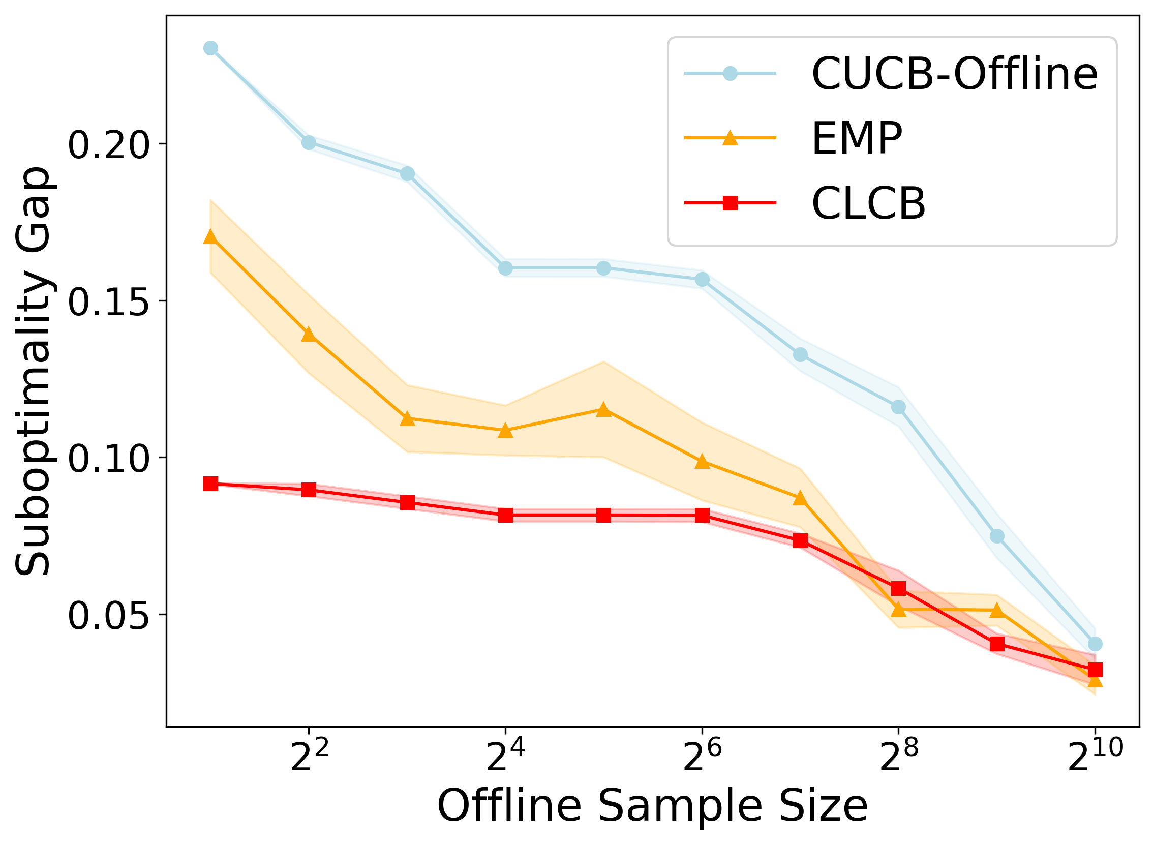
(a) Synthetic Dataset

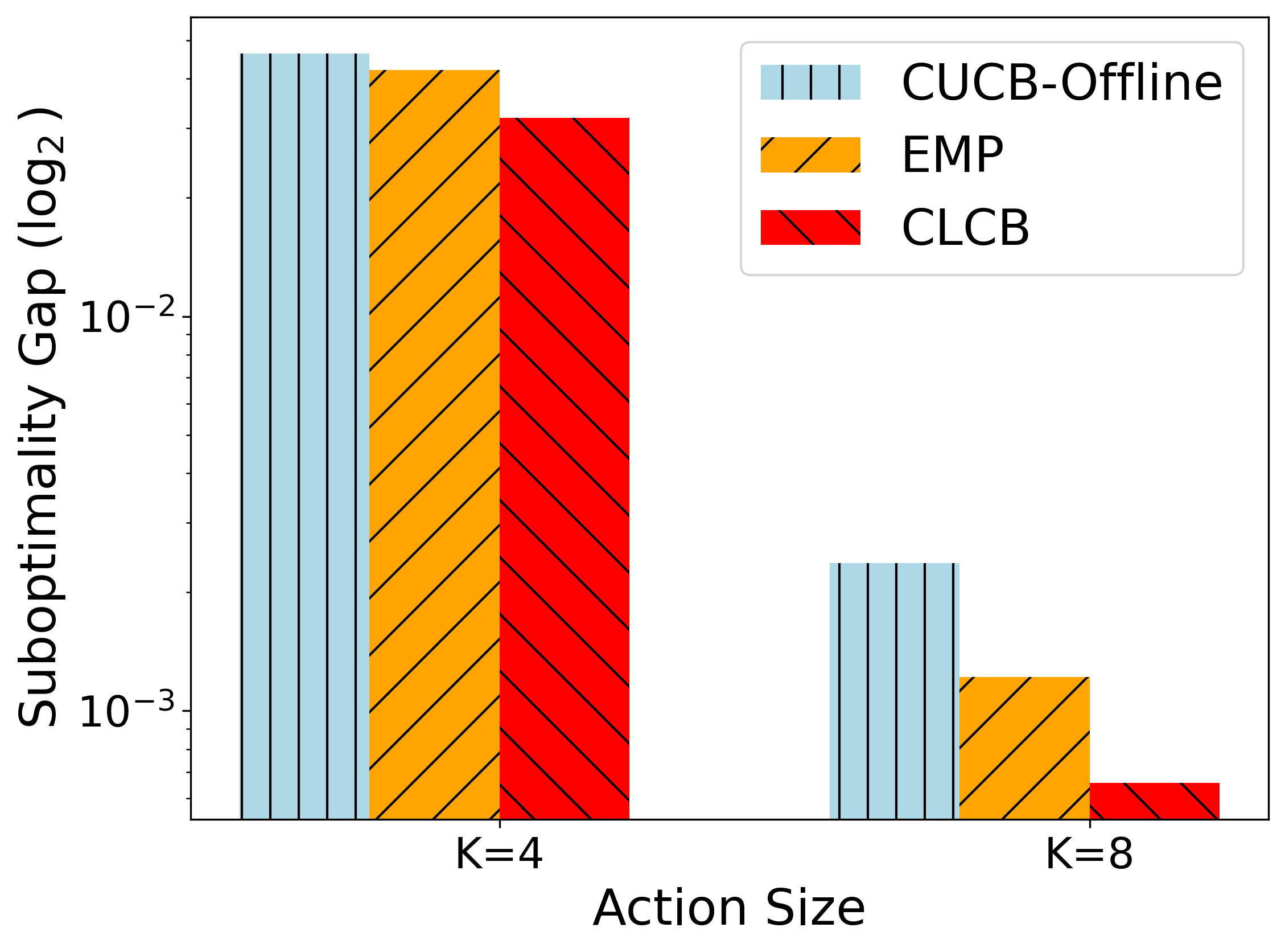
(b) Real-world Dataset

Figure 1: Suboptimality gaps for cascading bandit application.

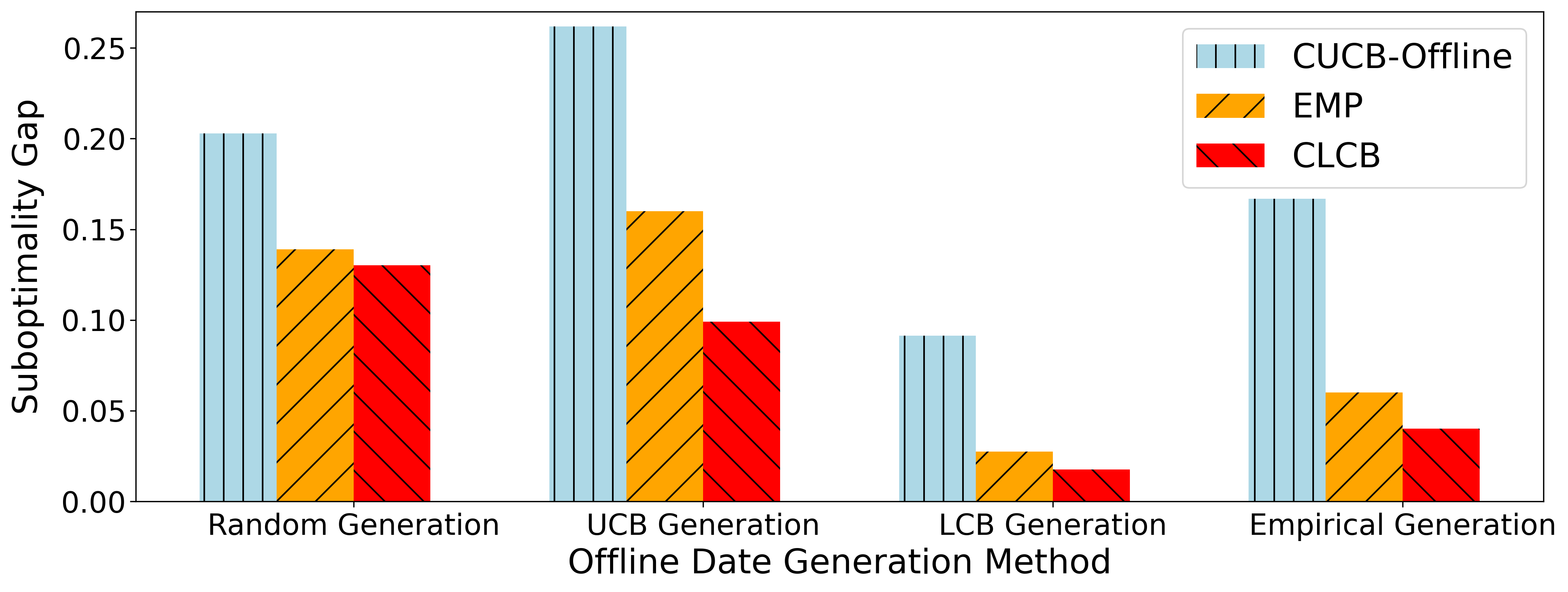
Figure 2: Comparison of different offline data generation methods.

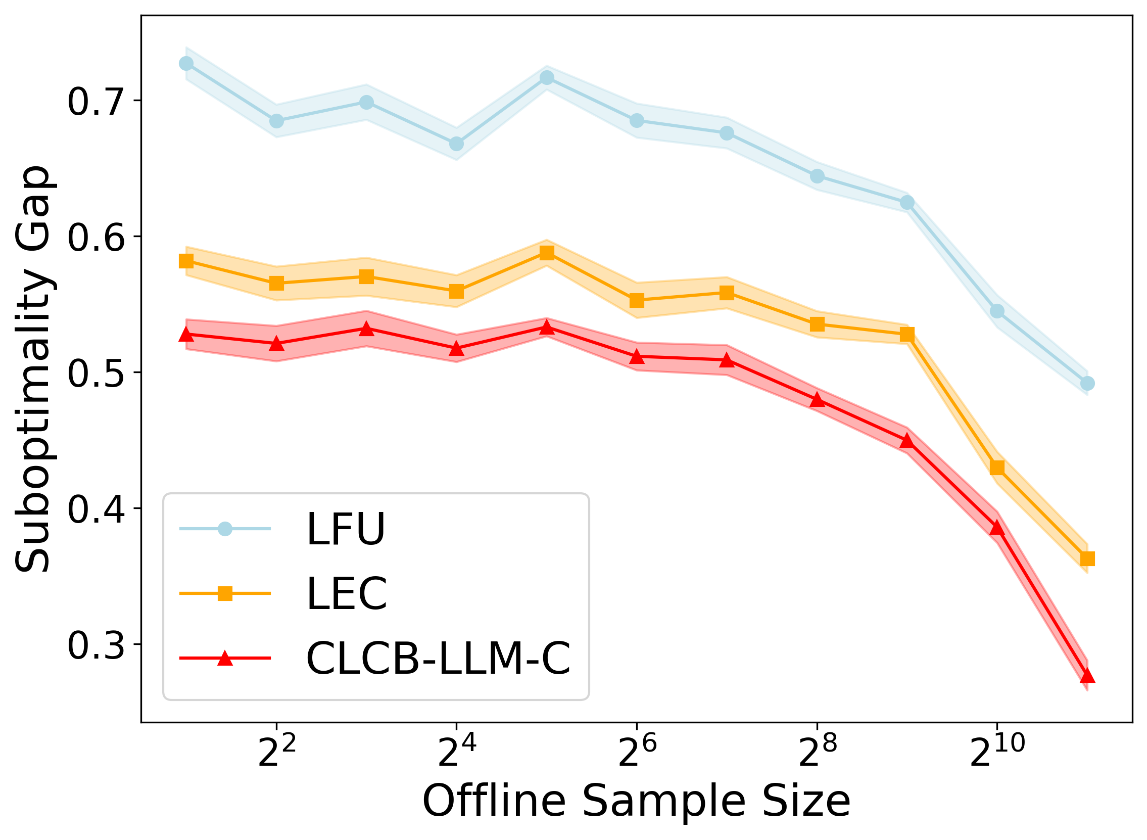
(a) Synthetic Dataset

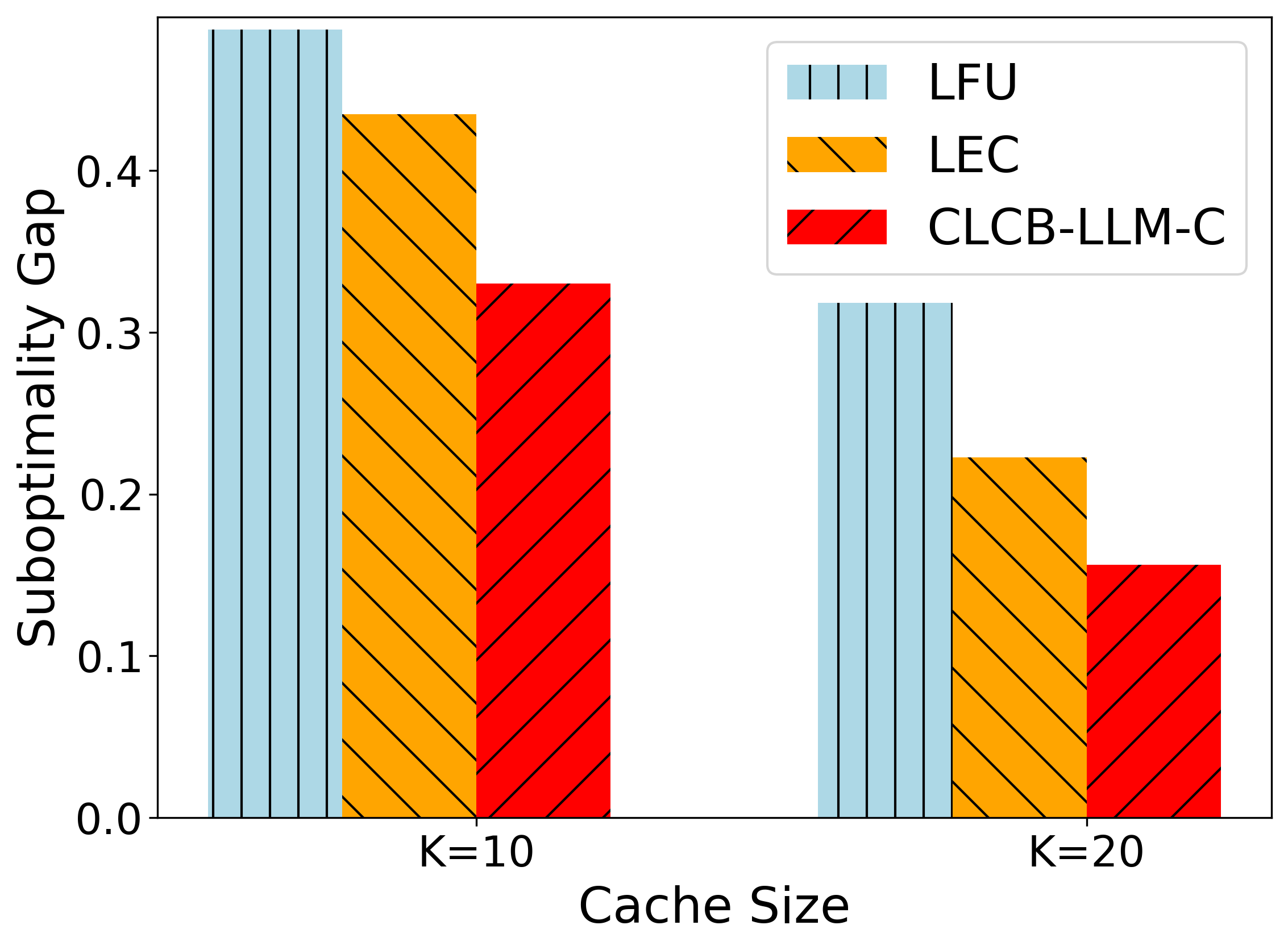
(b) Real-world Dataset

Figure 3: Suboptimality gaps for LLM cache application.

We now present experimental results on both synthetic and real-world datasets. For cascading bandits on the application of learning to rank, in the synthetic setting, item parameters $\mu_{i}$ are drawn from $U[0,1]$, and in each round $t$, a ranked list $S_{t}$ of $K$ items is randomly sampled. Fig. 1(a) shows that compared to CUCB-Offline [8], which is an offline adaptation of CUCB for our setting, and EMP [119], CLCB (Algorithm˜1) reduces suboptimality gaps by 47.75% and 20.02%, respectively. For real-world evaluation, we use the Yelp dataset, where users rate businesses. We randomly select $m=200$ rated items per user and recommend up to $K$ items to maximize the probability of user engagement. The unknown probability $\mu_{i}$ is derived from Yelp, and cascading feedback is collected. Fig. 1(b) compares suboptimality gaps over $n=100$ rounds for $K=4,8$ , with a logarithmic scale on the y-axis. Note that as $K$ increases, the expected reward also changes, thus reducing suboptimality gaps. CLCB consistently achieves the lowest suboptimality gap.

Moreover, we generate offline datasets $\mathcal{D}$ with $n=100$ in four different ways: random sampling, UCB-based generation, LCB-based generation, and empirical-based generation. For the UCB-based, LCB-based, and empirical-based data generation methods, we select the top $K=5$ arms with the largest UCB, LCB, and empirical reward means, respectively. It can be observed in Fig.˜2 that our method consistently maintains the smallest suboptimality gap. When using the UCB data generation method, our algorithm performs significantly better than the CUCB-Offline and EMP baselines, which aligns with our theoretical results.

Similarly, we conduct experiments in the LLM cache setting. In the synthetic setup, we simulate 100 distinct queries with a cache size of 40, following a power-law frequency distribution ($\alpha=0.9$) as in [34]. As shown in Fig. 3(a), our CLCB-LLM-C algorithm outperforms LFU [34] and LEC [34], achieving at least 1.32$\times$ improvement. For real-world evaluation, we use the SciQ dataset [120]. We evaluate GPT-4-o with the “o200k_base” encoding with cache sizes $K=10$ and $K=20$, where cost is defined by OpenAI’s API pricing with the tiktoken library [121]. Fig. 3(b) shows that CLCB-LLM-C (Algorithm˜3) reduces costs by up to 36.01% and 20.70%, compared to LFU and LEC. Moreover, a larger $K$ shows a lower suboptimality gap, which is consistent with Theorem˜3. Further details on experimental setups, results, and additional comparisons can be found in Appendix G.

The appendix is organized as follows.

• In Appendix˜A, we prove the upper bound of the suboptimal gap

  • under the infinity-norm TPM data coverage condition (˜3)

  • under 1-norm TPM data coverage condition (˜4).

• In Appendix˜B, we prove

  • the lower bound of suboptimal gap for the $k$-path problem with semi-bandit feedback.

• In Appendix˜C, we prove

  • the gap upper bound for the offline learning problem in cascading bandits.

• In Appendix˜D, we prove

  • the standard gap upper bound of for offline learning in LLM cache

  • the improved gap upper bound for offline learning in LLM cache

  • the improved regret upper bound for online streaming LLM cache

• In Appendix˜E, we prove

  • the gap upper bound for the influence maximization under the node-level feedback.

• In Appendix˜F, we prove auxiliary lemmas that serve as important ingredients for our analysis.

• In Appendix˜G, we provide the additional experimental results.

Appendix A Proof for the Upper Bound Result

Proof of Theorem˜1.

We first show the regret bound under the infinity-norm TPM data coverage condition (˜3):

Let $N_{i}(\mathcal{D})$ be the counter for arm $i$ as defined in line 3 of Algorithm˜1, given the dataset $\mathcal{D}$ and the failure probability $\delta$.

Let $\hat{\bm{\mu}}(\mathcal{D})=\left(\hat{\mu}_{1}(\mathcal{D},\delta),...,\hat{\mu}_{m}(\mathcal{D},\delta)\right)$ be the empirical mean defined in line 4 of Algorithm˜1.

Let $\underaccent{\bar}{\bmu}(\mathcal{D},\delta)=\left(\underaccent{\bar}{\mu}_{1}(\mathcal{D},\delta),...,\underaccent{\bar}{\mu}_{m}(\mathcal{D},\delta)\right)$ be the LCB vector defined in line 5 of Algorithm˜1.

Let $\hat{S}(\mathcal{D},\delta)$ be the action returned by Algorithm˜1 in line 7.

Let $p_{i}^{\mathbb{D}_{\text{arm}},\mathbb{D}_{\mathcal{S}}}$ be the data collecting probability that for arm $i$, i.e., the probability of observing arm $i$ in each offline data.

Let $\tilde{S}^{*}=\{i\in[m]:p_{i}^{\mathbb{D}_{\text{out}},S^{*}}>0\}$ be the arms that can be triggered by the optimal action $S^{*}$ and $p^{*}=\min_{i\in\tilde{S}^{*}}p_{i}^{\mathbb{D}_{\text{arm}},\mathbb{D}_{\mathcal{S}}}$ be the minimum data collection probability.

We first define the events $\mathcal{E}_{\text{arm}}$ and $\mathcal{E}_{\text{counter}}$ as follows.

$$\mathcal{E}_{\text{arm}} \vcentcolon=\left\{\left|\hat{\mu}_{i}(\mathcal{D})-\mu_{i}\right|\leq\sqrt{\frac{\log(\frac{2mn}{\delta})}{2N_{i}(\mathcal{D})}}\text{ for any }i\in[m]\right\}$$ (13)

$$\mathcal{E}_{\text{counter}} \vcentcolon=\left\{N_{i}(\mathcal{D})\geq\frac{n\cdot p_{i}^{\mathbb{D}_{\text{arm}},\mathbb{D}_{\mathcal{S}}}}{2}\text{ for any }i\in\tilde{S}^{*}\,\middle|\,n\geq\frac{8\log\frac{m}{\delta}}{p^{*}}\right\}$$ (14)

When $n\geq\frac{8\log\frac{m}{\delta}}{p^{*}}$ and under the events $\mathcal{E}_{\text{arm}}$ and $\mathcal{E}_{\text{counter}}$, we have the following gap decomposition:

$$\alpha r(S^{*};\bm{\mu})-r\left(\hat{S}(\mathcal{D},\delta);\bm{\mu}\right)$$ (15)

$$\overset{(a)}{=}\underbrace{\alpha r(S^{*};\bm{\mu})-\alpha r\left(S^{*};\underaccent{\bar}{\bmu}(\mathcal{D},\delta)\right)}_{\text{uncertainty gap}}$$ (16)

$$+\underbrace{\alpha r\left(S^{*};\underaccent{\bar}{\bmu}(\mathcal{D},\delta)\right)-r\left(\hat{S}(\mathcal{D},\delta);\underaccent{\bar}{\bmu}(\mathcal{D},\delta)\right)}_{\text{oracle gap}}+\underbrace{r\left(\hat{S}(\mathcal{D},\delta);\underaccent{\bar}{\bmu}(\mathcal{D},\delta)\right)-r\left(\hat{S}(\mathcal{D},\delta);\bm{\mu}\right)}_{\text{pessimism gap}}$$

$$\overset{(b)}{\leq}\alpha\left(r(S^{*};\bm{\mu})-r\left(S^{*};\underaccent{\bar}{\bmu}(\mathcal{D},\delta)\right)\right)$$ (17)

$$\overset{(c)}{\leq}\alpha B_{1}\sum_{i\in[m]}p_{i}^{\mathbb{D}_{\text{arm}},S^{*}}\left(\mu_{i}-\underaccent{\bar}{\mu}_{i}(\mathcal{D},\delta)\right)$$ (18)

$$\overset{(d)}{\leq}2\alpha B_{1}\sum_{i\in[m]}p_{i}^{\mathbb{D}_{\text{arm}},S^{*}}\sqrt{\frac{\log(\frac{2mn}{\delta})}{2N_{i}(\mathcal{D})}}$$ (19)

$$\overset{(e)}{\leq}2\alpha B_{1}\sum_{i\in[m]}p_{i}^{\mathbb{D}_{\text{arm}},S^{*}}\sqrt{\frac{\log(\frac{2mn}{\delta})}{n\cdot p_{i}^{\mathbb{D}_{\text{arm}},\mathbb{D}_{\mathcal{S}}}}}$$ (20)

$$\leq 2\alpha B_{1}\sum_{i\in[m]}\sqrt{p_{i}^{\mathbb{D}_{\text{arm}},S^{*}}}\sqrt{\frac{\log(\frac{2mn}{\delta})\cdot p_{i}^{\mathbb{D}_{\text{arm}},S^{*}}}{n\cdot p_{i}^{\mathbb{D}_{\text{arm}},\mathbb{D}_{\mathcal{S}}}}}$$ (21)

$$\overset{(f)}{\leq}2\alpha B_{1}\bar{K}^{*}_{2}\sqrt{\frac{2\log(\frac{2mn}{\delta})\cdot C^{*}_{\infty}}{n}},$$ (22)

where inequality (a) is due to adding and subtracting $\alpha r\left(S^{*};\underaccent{\bar}{\bmu}(\mathcal{D},\delta)\right)$ and $r\left(\hat{S}(\mathcal{D},\delta);\underaccent{\bar}{\bmu}(\mathcal{D},\delta)\right)$, inequality (b) is due to oracle gap $\leq 0$ by Eq.˜1 as well as pessimism gap $\leq 0$ by monotonicity (˜1) and Lemma˜5, inequality (c) is due to 1-norm TPM smoothness condition (˜2), inequality (d) is due to Lemma˜5, inequality (e) is due to event $\mathcal{E}_{counter}$, inequality (f) is due to infinity-norm TPM data coverage condition (˜3).

Next, we show the regret bound under the 1-nrom TPM data coverage condition (˜4).

When $n\geq\frac{8\log\frac{m}{\delta}}{p^{*}}$ and under the events $\mathcal{E}_{\text{arm}}$ and $\mathcal{E}_{\text{counter}}$, we follow the proof from Eq.˜15 to Eq.˜21 and proceed as:

$$\alpha r(S^{*};\bm{\mu})-r\left(\hat{S}(\mathcal{D},\delta);\bm{\mu}\right)$$ (23)

$${=}\underbrace{\alpha r(S^{*};\bm{\mu})-\alpha r\left(S^{*};\underaccent{\bar}{\bmu}(\mathcal{D},\delta)\right)}_{\text{uncertainty gap}}$$ (24)

$$+\underbrace{\alpha r\left(S^{*};\underaccent{\bar}{\bmu}(\mathcal{D},\delta)\right)-r\left(\hat{S}(\mathcal{D},\delta);\underaccent{\bar}{\bmu}(\mathcal{D},\delta)\right)}_{\text{oracle gap}}+\underbrace{r\left(\hat{S}(\mathcal{D},\delta);\underaccent{\bar}{\bmu}(\mathcal{D},\delta)\right)-r\left(\hat{S}(\mathcal{D},\delta);\bm{\mu}\right)}_{\text{pessimism gap}}$$

$${\leq}\alpha\left(r(S^{*};\bm{\mu})-r\left(S^{*};\underaccent{\bar}{\bmu}(\mathcal{D},\delta)\right)\right)$$ (25)

$${\leq}\alpha B_{1}\sum_{i\in[m]}p_{i}^{\mathbb{D}_{\text{arm}},S^{*}}\left(\mu_{i}-\underaccent{\bar}{\mu}_{i}(\mathcal{D},\delta)\right)$$ (26)

$$\leq 2\alpha B_{1}\sum_{i\in[m]}\sqrt{p_{i}^{\mathbb{D}_{\text{arm}},S^{*}}}\sqrt{\frac{2\log(\frac{2mn}{\delta})\cdot p_{i}^{\mathbb{D}_{\text{arm}},S^{*}}}{n\cdot p_{i}^{\mathbb{D}_{\text{arm}},\mathbb{D}_{\mathcal{S}}}}}$$ (27)

$$\overset{(a)}{\leq}2\alpha B_{1}\sqrt{\sum_{i\in[m]}p_{i}^{\mathbb{D}_{\text{arm}},S^{*}}}\sqrt{\sum_{i\in[m]}\frac{2\log(\frac{2mn}{\delta})\cdot p_{i}^{\mathbb{D}_{\text{arm}},S^{*}}}{n\cdot p_{i}^{\mathbb{D}_{\text{arm}},\mathbb{D}_{\mathcal{S}}}}}$$ (28)

$$\overset{(b)}{\leq}2\alpha B_{1}\sqrt{\frac{2\bar{K}^{*}C_{1}^{*}\log(\frac{2mn}{\delta})}{n}},$$ (29)

where inequality (a) is due to Cauchy Schwarz inequality, and inequality (b) is due to 1-norm TPM data coverage condition ˜4.

The final step is to show event $\mathcal{E}_{\text{arm}}$ and $\mathcal{E}_{\text{counter}}$ hold with high probability. By Lemma˜5 and Lemma˜6, event $\mathcal{E}_{\text{arm}}$ and $\mathcal{E}_{\text{counter}}$ both hold with probability at least with $1-\delta$. By setting $\delta^{\prime}=\delta/2$ concludes the proof.

∎

Appendix B Proof for the Lower Bound Result

Proof of Theorem˜2.

Let $\Delta\in[0,\frac{1}{4}]$ be a gap to be tuned later and let $C_{\infty}^{*}\geq 2$. We consider a $k$-path problem with two problem instances ${\mathcal{P}}_{1}$ and ${\mathcal{P}}_{2}$, where $m/k$ path’s mean vectors are $\bm{\mu}_{1}=(\frac{1}{2},\frac{1}{2}-\Delta,0,...,0)\in\mathbb{R}^{m/k}$ and $\bm{\mu}_{2}=(\frac{1}{2},\frac{1}{2}+\Delta,0,...,0)\in\mathbb{R}^{m/k}$, respectively. For the data collecting distribution, $\mathbb{D}_{\mathcal{S}}$ follows $\bm{p}=(\frac{1}{C_{\infty}^{*}},1-\frac{1}{C_{\infty}^{*}},0,...,0)$ for both ${\mathcal{P}}_{1}$ and ${\mathcal{P}}_{2}$. We have that the optimal action $S_{1}^{*}=(1,2,...,k)$ for ${\mathcal{P}}_{1}$ and $S_{2}^{*}=(k+1,k+2,...,2k)$ for ${\mathcal{P}}_{2}$.

For the triggering probability, $p_{i}^{{\mathcal{P}}_{1},S^{*}}=1$ for $i=1,...,k$ and $0$ otherwise and $p_{i}^{{\mathcal{P}}_{2},S^{*}}=1$ for $i=k+1,...,2k$ and $0$ otherwise.

We then show that both problem instances ${\mathcal{P}}_{1},{\mathcal{P}}_{2}$ satisfy ˜3. For ${\mathcal{P}}_{1}$ and ${\mathcal{P}}_{2}$, we have

$$\max_{i\in[m]}\frac{p_{i}^{{\mathcal{P}}_{1},S^{*}}}{p_{i}^{{\mathcal{P}}_{1},\mathcal{D}_{\mathcal{S}}}} =\frac{1}{\frac{1}{C_{\infty}^{*}}}=C_{\infty}^{*},$$ (30)

$$\max_{i\in[m]}\frac{p_{i}^{{\mathcal{P}}_{2},S^{*}}}{p_{i}^{{\mathcal{P}}_{2},\mathcal{D}_{\mathcal{S}}}} =\frac{1}{1-\frac{1}{C_{\infty}^{*}}}\overset{(a)}{\leq}C_{\infty}^{*},$$ (31)

where inequality $(a)$ is due to $C_{\infty}^{*}\geq 2$.

Let us define suboptimality gap of any action $\hat{S}$ as:

$$g(\hat{S};\bm{\mu})\vcentcolon=r(S^{*}(\bm{\mu});\bm{\mu})-r(\hat{S};\bm{\mu})$$ (32)

where $S^{*}(\bm{\mu})$ is the optimal super arm under $\bm{\mu}$.

For any action $\hat{S}\in\mathcal{S}$, we have

$$g(\hat{S};\bm{\mu}_{1})+g(\hat{S};\bm{\mu}_{2})\geq k\Delta$$ (33)

Recall that $A(\mathcal{D})$ is the action returned by algorithm $A$ and we use the Le Cam’s method [122]:

$$\inf_{A}\,\,\,\,\sup_{(\mathbb{D}_{\text{arm}},\mathbb{D}_{\mathcal{S}})\in\text{k-path}(m,k,C_{\infty}^{*})}\mathbb{E}_{\mathcal{D}\sim\mathbb{D}(\mathbb{D}_{\text{arm}},\mathbb{D}_{\mathcal{S}})}[r(S^{*};\mu)-r(A(\mathcal{D});\mu)]$$ (34)

$$\geq\inf_{A}\sup_{\bm{\mu}\in\bm{\mu}_{1},\bm{\mu}_{2}}\mathbb{E}_{\mathcal{D}}[g(A(\mathcal{D});\bm{\mu})]$$ (35)

$$\overset{(a)}{\geq}\inf_{A}\frac{1}{2}\left(\mathbb{E}_{\bm{p}\otimes\bm{\mu}_{1}}[A(\mathcal{D});\bm{\mu}_{1})]+\mathbb{E}_{\bm{p}\otimes\bm{\mu}_{2}}[g(A(\mathcal{D});\bm{\mu}_{2})]\right)$$ (36)

$$\overset{(b)}{\geq}\frac{k\Delta}{4}\exp\left(-\mathrm{KL}\left(\mathbb{P}_{\bm{p}\bigotimes\bm{\mu}_{1}}||\mathbb{P}_{\bm{p}\bigotimes\bm{\mu}_{2}}\right)\right),$$ (37)

where inequality (a) is due to $\max{a,b}\geq(a+b)/2$, and inequality (b) is due to the following derivation:

Let event $\mathcal{E}=\{g(A(\mathcal{D});\bm{\mu}_{1})\leq\frac{k\Delta}{2}\}$. On $\neg\mathcal{E}$ it holds that $g(A(\mathcal{D});\bm{\mu}_{1})\geq\frac{k\Delta}{2}$ and on $\mathcal{E}$ it holds that $g(A(\mathcal{D});\bm{\mu}_{2})\geq k\Delta-g(A(\mathcal{D});\bm{\mu}_{1})\geq\frac{k\Delta}{2}$. Thus, we have:

$$\inf_{A}\frac{1}{2}\left(\mathbb{E}_{\bm{p}\otimes\bm{\mu}_{1}}[g(A(\mathcal{D});\bm{\mu}_{1})]+\mathbb{E}_{\bm{p}\otimes\bm{\mu}_{2}}[g(A(\mathcal{D});\bm{\mu}_{2})]\right)$$ (38)

$${\geq}\frac{k\Delta}{4}\left(\mathbb{P}_{\bm{p}\otimes\bm{\mu}_{1}}(\neg\mathcal{E})+\mathbb{P}_{\bm{p}\otimes\bm{\mu}_{2}}(\mathcal{E})\right)$$ (39)

$$\overset{(a)}{\geq}\frac{k\Delta}{8}\exp\left(-\mathrm{KL}\left(\mathbb{P}_{\bm{p}\bigotimes\bm{\mu}_{1}}||\mathbb{P}_{\bm{p}\bigotimes\bm{\mu}_{2}}\right)\right)$$ (40)

$$\overset{(b)}{\geq}\frac{k}{8e}\min\left(\frac{1}{4},\sqrt{\frac{C_{\infty}^{\star}}{20n}}\right)$$ (41)

where inequality (a) is due to Lemma˜8 and inequality (b) comes from: $\mathrm{KL}\left(\mathbb{P}_{\bm{p}\otimes\bm{\mu}_{1}}\|\mathbb{P}_{\bm{p}\otimes\bm{\mu}_{2}}\right)\leq\frac{n\mathrm{KL}\left(\mathbb{P}_{\bm{\mu}_{1}}\|\mathbb{P}_{\bm{\mu}_{2}}\right)}{C_{\infty}^{\star}}\leq\frac{n(2\Delta)^{2}}{C_{\infty}^{\star}\left(1/4-\Delta^{2}\right)}\leq 20n\Delta^{2}/C_{\infty}^{\star}$. Here we use the fact that each arm in the path are fully dependent Bernoulli random variables, $\mathrm{KL}\left(\mathrm{Bern}(p)||\mathrm{Bern}(q)\right)\leq\frac{(p-q)^{2}}{q(1-q)}$ and that $\Delta\in[0,\frac{1}{4}]$. By taking $\Delta=\min\left(\frac{1}{4},\sqrt{\frac{C_{\infty}^{\star}}{20n}}\right)$ yields concludes Theorem˜2. ∎

Appendix C Proof for the Application of Offline Learning for Cascading Bandits

Proof of Corollary˜1.

For the cascading bandit application, we need to prove how it satisfies the monotonicity condition (˜1), the 1-norm TPM condition (˜2), the 1-norm data coverage condition (˜4), and then settle down the corresponding smoothness factor $B_{1}$, data coverage coefficient $C_{1}^{*}$, action size $\bar{K}^{*}$.

Algorithm 5 CLCB-Cascade: Combinatorial Lower Confidence Bound Algorithm for Cascading Bandits

1:Input: Dataset $\mathcal{D}=\left\{\left(S_{t},\tau_{t},(X_{t,i})_{i\in\tau_{t}}\right)\right\}_{t=1}^{n}$, cardinality $k>0$, solver Top-k, probability $\delta$.

2:for arm $i\in[m]$ do

3:  Calculate counter $N_{i}=\sum_{t=1}^{n}\mathbb{I}\{i\in\tau_{t}\}$;

4:  Calculate empirical mean $\hat{\mu}_{i}=\frac{\sum_{t=1}^{n}\mathbb{I}\{i\in\tau_{t}\}X_{t,i}}{N_{i}}$;

5:  Calculate LCB $\underaccent{\bar}{\mu}_{i}=\hat{\mu}_{i}-\sqrt{\frac{\log(\frac{2mn}{\delta})}{2N_{i}}}$.

6:end for

7:Call oracle $\hat{S}=\texttt{Top-k}(\underaccent{\bar}{\mu}_{1},...,\underaccent{\bar}{\mu}_{m})$.

8:Return: $\hat{S}$.

For the monotonicity condition (˜1), the 1-norm TPM condition (˜2), Lemma 1 in Wang and Chen [9] yields $B_{1}=1$.

For the 1-norm data coverage condition (˜4), recall that we assume the arm means are in descending order $\mu_{1}\geq\mu_{2}\geq...\geq\mu_{m}$, therefore we have $S^{*}=(1,2,...,k)$, and

$$p_{i}^{\mathbb{D}_{\text{arm}},S^{*}}=\begin{cases}\prod_{j=1}^{i-1}(1-\mu_{j}),\text{ if $i\leq k$,}\\ 0,\text{ else if $i\geq k+1$}.\end{cases}$$ (43)

As for $p_{i}^{\mathbb{D}_{\text{arm}},\mathbb{D}_{\mathcal{S}}}$, we have

$$p_{i}^{\mathbb{D}_{\text{arm}},\mathbb{D}_{\mathcal{S}}}\geq\sum_{j=1}^{k}q_{ij}(1-\mu_{1})^{j-1},$$ (44)

where $q_{ij}$ is the probability that arm $i$ is sampled at the $j$-th position of the random ranked list sampled by the experimenter.

By math calculation, we have

$$C_{1}^{*}=\sum_{i\in[m]}\frac{p_{i}^{\mathbb{D}_{\text{arm}},S^{*}}}{p_{i}^{\mathbb{D}_{\text{arm}},\mathbb{D}_{\mathcal{S}}}}\leq\sum_{i=1}^{k}\frac{\prod_{j=1}^{i-1}(1-\mu_{j})}{\sum_{j=1}^{k}q_{ij}(1-\mu_{1})^{j-1}}$$ (45)

and

$$\bar{K}^{*}=\sum_{i\in[m]}p_{i}^{\mathbb{D}_{\text{arm}},S^{*}}\leq\sum_{i\in[k]}1=k$$ (46)

Plugging $B_{1}=1,C_{1}^{*}=\sum_{i=1}^{k}\frac{\prod_{j=1}^{i-1}(1-\mu_{j})}{\sum_{j=1}^{k}q_{ij}(1-\mu_{1})^{j-1}},\bar{K}^{*}=k$ into our general result Theorem˜1 yields the general result of Corollary˜1.

When we assume that the data collecting distribution $\mathbb{D}_{\mathcal{S}}$ follows the uniform distribution from all possible ordered lists $\mathcal{S}=\{(a_{1},...,a_{k}):a_{i}\in[m]\text{ for all }i\in[m]\text{, and }a_{i}\neq a_{j}\text{ for all }i\neq j\}$. Then we have $q_{i,j}=\frac{1}{m}$, and using Eq.˜44 we have

$$p_{i}^{\mathbb{D}_{\text{arm}},\mathbb{D}_{\mathcal{S}}}\geq\sum_{j=1}^{k}\frac{(1-\mu_{1})^{j-1}}{m}=\frac{1-(1-\mu_{1})^{k}}{\mu_{1}\cdot m}$$ (47)

We can use Eq.˜45 and Eq.˜43 to bound

$$C_{1}^{*} =\sum_{i\in[m]}\frac{p_{i}^{\mathbb{D}_{\text{arm}},S^{*}}}{p_{i}^{\mathbb{D}_{\text{arm}},\mathbb{D}_{\mathcal{S}}}}\leq\sum_{i\in[m]}\frac{p_{i}^{\mathbb{D}_{\text{arm}},S^{*}}}{\frac{1-(1-\mu_{1})^{k}}{\mu_{1}\cdot m}}$$ (48)

$$\leq\frac{\sum_{j=1}^{k}(1-\mu_{k})^{j}}{\frac{1-(1-\mu_{1})^{k}}{\mu_{1}\cdot m}}$$ (49)

$$=\frac{\frac{1-(1-\mu_{k})^{k}}{\mu_{k}}}{\frac{1-(1-\mu_{1})^{k}}{\mu_{1}\cdot m}}$$ (50)

$$\leq\frac{\mu_{1}\cdot m}{\mu_{k}}.$$ (51)

Plugging $B_{1}=1,C_{1}^{*}=\frac{\mu_{1}\cdot m}{\mu_{k}},\bar{K}^{*}=k$ into our general result Theorem˜1 concludes Corollary˜1.

∎

Appendix D Algorithm and Proof for the LLM Cache Application

D.1 Offline Learning for the LLM Cache under the Standard CMAB-T View

For this LLM cache problem, we first show the corresponding base arms, super arm, and triggering probability. Then we prove this problem satisfies the 1-norm TPM smoothness condition (˜2) and 1-norm TPM data coverage condition (˜4). Finally, we give the upper bound result by using Theorem˜1.

From the CMAB-T point of view, we have $2m$ base arms: the first $m$ arms correspond to the unknown costs $c(q)\in[0,1]$ for $q\in{\mathcal{Q}}$, and the last $m$ arms corresponds to the arrival probability $p(q)\in[0,1]$ for $q\in{\mathcal{Q}}$.

Let us denote $\bm{c}=(c(q))_{q\in{\mathcal{Q}}}$ and $\bm{p}=(p(q))_{q\in{\mathcal{Q}}}$ for convenience.

Recall that we treat the queries $S\in\mathcal{S}$ outside the cache $\mathcal{M}$ as the super arm, where $\mathcal{S}=\{{\mathcal{Q}}-\mathcal{M}:\mathcal{M}\subseteq{\mathcal{Q}},|\mathcal{M}|\leq k\}$.

We can write the expected cost for each super arm $S\in\mathcal{S}$ as $c(S;\bm{c},\bm{p})=\sum_{q\in S}p(q)c(q)$.

Then we know that $S^{*}=\operatorname*{argmax}_{S\in\mathcal{S}}c(S;\bm{c},\bm{p})$, which contains the top $m-k$ queries regarding $p(q)c(q)$.

For the triggering probability, we have that, for any $S\in\mathcal{S}$, the triggering probability for unknown costs $p_{q,c}^{\mathbb{D}_{\text{arm}},S}=p(q)$ for $q\in S$ and $0$ otherwise. The triggering probability for unknown arrival probability $p_{q,p}^{\mathbb{D}_{\text{arm}},S}=1$ for all $q\in{\mathcal{Q}}$.

Now we can prove that this problem satisfies the 1-norm TPM smoothness condition (˜2) with $B_{1}=1$. That is, for any $S\in\mathcal{S}$, any $\bm{p},\bm{p}^{\prime},\bm{c},\bm{c}^{\prime}\in[0,1]^{m}$, we have

$$|c(S;\bm{c},\bm{p})-c(S;\bm{c}^{\prime},\bm{p}^{\prime})| =|c(S;\bm{c},\bm{p})-c(S;\bm{c}^{\prime},\bm{p})+c(S;\bm{c}^{\prime},\bm{p})-c(S;\bm{c}^{\prime},\bm{p}^{\prime})|$$ (52)

$$\leq|c(S;\bm{c},\bm{p})-c(S;\bm{c}^{\prime},\bm{p})|+|c(S;\bm{c}^{\prime},\bm{p})-c(S;\bm{c}^{\prime},\bm{p}^{\prime})|$$ (53)

$$=\left|\sum_{q\in S}p(q)c(q)-p(q)c^{\prime}(q)\right|+\left|\sum_{q\in S}p(q)c^{\prime}(q)-p^{\prime}(q)c^{\prime}(q)\right|$$ (54)

$$\leq\sum_{q\in S}p(q)\left|c(q)-c^{\prime}(q)\right|+\sum_{q\in S}c^{\prime}(q)\left|p(q)-p^{\prime}(q)\right|$$ (55)

$$\leq\sum_{q\in S}p(q)\left|c(q)-c^{\prime}(q)\right|+\sum_{q\in{\mathcal{Q}}}\left|p(q)-p^{\prime}(q)\right|$$ (56)

Next, we prove that this problem satisfies the 1-norm TPM data coverage condition (˜3).

Let $\nu(q)=\Pr_{\mathcal{M}\sim\mathbb{D}_{\mathcal{S}}}\left[q\notin\mathcal{M}\right]$ be the probability that $q$ is not sampled in the experimenter’s cache $\mathcal{M}\sim\mathbb{D}_{\mathcal{S}}$. Then the data collecting probability for unknown costs $p_{q,c}^{\mathbb{D}_{\text{arm}},\mathbb{D}_{\mathcal{S}}}=p(q)\nu(q)$ and $p_{q,p}^{\mathbb{D}_{\text{arm}},\mathbb{D}_{\mathcal{S}}}=1$ for unknown arrival probability, for $q\in{\mathcal{Q}}$. We can prove that the LLM cache satisfies ˜4 by

$$\sum_{q\in{\mathcal{Q}}}\left(\frac{p_{q,c}^{\mathbb{D}_{\text{arm}},S^{*}}}{p_{q,c}^{\mathbb{D}_{\text{arm}},\mathbb{D}_{\mathcal{S}}}}+\frac{p_{q,p}^{\mathbb{D}_{\text{arm}},S^{*}}}{p_{q,p}^{\mathbb{D}_{\text{arm}},\mathbb{D}_{\mathcal{S}}}}\right)=\sum_{q\in{\mathcal{Q}}}\left(\frac{p(q)\mathbb{I}\{q\in S^{*}\}}{p(q)\nu(q)}+1\right)\leq\sum_{q\in S^{*}}\frac{1}{\nu(q)}+m=C_{1}^{*}.$$ (57)

Finally, we have $\bar{K}^{*}=\sum_{q\in{\mathcal{Q}}}\left(p_{q,c}^{\mathbb{D}_{\text{arm}},S^{*}}+p_{q,p}^{\mathbb{D}_{\text{arm}},S^{*}}\right)=\sum_{q\in{\mathcal{Q}}}p(q)\mathbb{I}\{q\in S^{*}\}+\sum_{q\in{\mathcal{Q}}}1\leq 1+m$.

Plugging into Theorem˜1 with $B_{1}=1$, $C_{1}^{*}=\sum_{q\in S^{*}}\frac{1}{\nu(q)}+m$, $\bar{K}^{*}=1+m$, we have the following suboptimality upper bound.

Lemma 1 (Standard Upper Bound for LLM Cache).

For LLM cache bandit with a dataset $\mathcal{D}$ of $n$ data samples, let $\mathcal{M}^{*}$ be the optimal cache and suppose $n\geq\frac{8\log(\frac{1}{\delta})}{\min_{q\in{\mathcal{Q}}-\mathcal{M}^{*}}p(q)\nu(q)}$, where $\nu(q)$ is the probability that query $q$ is not included in each offline sampled cache. Let $\hat{M}$ be the cache returned by algorithm Algorithm˜2, then it holds with probability at least $1-\delta$ that

$$\mathrm{SubOpt}(\hat{\mathcal{M}};\alpha,\bm{c},\bm{p}) \vcentcolon=c(\mathcal{M}^{*};\bm{c},\bm{p})-c\left(\hat{\mathcal{M}};\bm{c},\bm{p}\right)$$ (58)

$$\leq 2\sqrt{\frac{2(m+1)\left(\sum_{q\in{\mathcal{Q}}-\mathcal{M}^{*}}\frac{1}{\nu(q)}+m\right)\log(\frac{4mn}{\delta})}{n}},$$ (59)

if the experimenter samples empty cache in each round as in [34] so that $\nu(q)=1$, it holds that $C_{1}^{*}\leq 2m$ and

$$\mathrm{SubOpt}(\hat{\mathcal{M}};\alpha,\bm{\mu}) \vcentcolon=c(\mathcal{M}^{*};\bm{p},\bm{c})-c\left(\hat{\mathcal{M}};\bm{p},\bm{c}\right)$$ (60)

$$\leq 2\sqrt{\frac{4m(m+1)\log(\frac{4mn}{\delta})}{n}}.$$ (61)

D.2 Improved Offline Learning for the LLM Cache by Leveraging the Full-feedback Property and the Vector-valued Concentration Inequality

Theorem 5 (Improved Upper Bound for LLM Cache).

For LLM cache bandit with a dataset $\mathcal{D}$ of $n$ data samples, let $\mathcal{M}^{*}$ be the optimal cache and suppose $n\geq\frac{8\log(\frac{1}{\delta})}{\min_{q\in{\mathcal{Q}}-\mathcal{M}^{*}}p(q)\nu(q)}$, where $\nu(q)$ is the probability that query $q$ is not included in each offline sampled cache. Let $\hat{M}$ be the cache returned by algorithm Algorithm˜2, then it holds with probability at least $1-\delta$ that

$$\mathrm{SubOpt}(\hat{\mathcal{M}};\alpha,\bm{\mu}) \vcentcolon=c(\mathcal{M}^{*};\bm{p},\bm{c})-c\left(\hat{\mathcal{M}};\bm{p},\bm{c}\right)$$ (62)

$$\leq 2\sqrt{\frac{2\sum_{q\in{\mathcal{Q}}-\mathcal{M}^{*}}{\frac{1}{\nu(q)}}\log(\frac{6mn}{\delta})}{n}}+2\sqrt{\frac{2m\log(\frac{3}{\delta})}{n}},$$ (63)

if the experimenter samples empty cache in each round as in [34] so that $\nu(q)=1$, it holds that $C_{1}^{*}\leq m$ and

$$\mathrm{SubOpt}(\hat{\mathcal{M}};\alpha,\bm{\mu}) \vcentcolon=c(\mathcal{M}^{*};\bm{p},\bm{c})-c\left(\hat{\mathcal{M}};\bm{p},\bm{c}\right)$$ (64)

$$\leq 4\sqrt{\frac{2m\log(\frac{6mn}{\delta})}{n}}.$$ (65)

In this section, we use an improved CMAB-T view by clustering $m$ arrival probabilities $p(q)$ as a vector-valued arm, which is fully observed in each data sample (observing $q$ means observing one hot vector $\bm{e}_{q}\in\{0,1\}^{m}$ with $1$ at the $q$-th entry and $0$ elsewhere).

Specifically, we have $m+1$ base arms: the first $m$ arms correspond to the unknown costs $c(q)$ for $q\in{\mathcal{Q}}$, and the last (vector-valued) arm corresponds to the arrival probability vector $(p(q))_{q\in{\mathcal{Q}}}$.

Let us denote $\bm{c}=(c(q))_{q\in{\mathcal{Q}}}$ and $\bm{p}=(p(q))_{q\in{\mathcal{Q}}}$ for convenience.

For the triggering probability, for any action $S$, we only consider unknown costs $p_{q,c}^{\mathbb{D}_{\text{arm}},S}=p(q)$ for $q\in S$ and $0$ otherwise.

For the 1-norm TPM smoothness condition (˜2), directly following Eq.˜56, we have that for any $S\in\mathcal{S}$, any $\bm{p},\bm{p}^{\prime},\bm{c},\bm{c}^{\prime}\in[0,1]^{m}$,

$$|c(S;\bm{c},\bm{p})-c(S;\bm{c}^{\prime},\bm{p}^{\prime})|\leq\sum_{q\in S}p(q)\left|c(q)-c^{\prime}(q)\right|+\sum_{q\in{\mathcal{Q}}}\left|p(q)-p^{\prime}(q)\right|=\sum_{q\in S}p(q)\left|c(q)-c^{\prime}(q)\right|+\left\lVert\bm{p}-\bm{p}^{\prime}\right\rVert_{1}$$ (66)

Recall that the empirical arrival probability vector is $\hat{\bm{p}}$ and the UCB of the cost is $\bar{\bm{c}}$.

Recall that $\hat{\mathcal{M}}=\operatorname*{argmax}_{|\mathcal{M}|=k}\sum_{q\in\mathcal{M}}\hat{p}(q)\bar{c}(q)$ given by line 7 in Algorithm˜3, which from the CMAB-T view, corresponds to the super arm $\hat{S}={\mathcal{Q}}-\hat{\mathcal{M}}=\operatorname*{argmin}_{S\in\mathcal{S}}c(S;\bar{\bm{c}},\hat{\bm{p}})$.

Since we treat $\bm{p}$ as a single vector-valued base arm and consider the cost function (and minimizing the cost) instead of the reward function (and maximizing the reward), we need a slight adaptation of the proof of Eq.˜15 as follows:

Recall that the dataset $\mathcal{D}=\left\{\left(\mathcal{M}_{t},q_{t},c_{t}\right)\right\}_{t=1}^{n}$.

Recall that $N_{c}(q)=\sum_{t=1}^{n}\mathbb{I}\{q=q_{t}\text{ and }q_{t}\notin\mathcal{M}_{t}\}$ is the number of times that $q$ is not in cache $\mathcal{M}_{t}$.

Recall that $\nu(q)$ is the probability that query $q$ is not included in each offline sampled cache $\mathcal{M}_{t}$.

Let $p^{*}=\min_{q\in{\mathcal{Q}}-\mathcal{M}^{*}}p(q)\nu(q)$ be the minimum data collecting probability.

First, we need a new concentration event for the vector-valued $\mathcal{E}_{arv}$ and two previous events as follows.

$$\mathcal{E}_{\text{arv}} \vcentcolon=\left\{\left\lVert\hat{\bm{p}}-\bm{p}\right\rVert_{1}\leq\sqrt{\frac{2m\log(\frac{2}{\delta})}{n}}\right\}$$ (67)

$$\mathcal{E}_{\text{arm}} \vcentcolon=\left\{\left|\hat{c}(q)-c(q)\right|\leq\sqrt{\frac{\log(\frac{2mn}{\delta})}{2N_{c}(q)}}\text{ for any }q\in{\mathcal{Q}}\right\}$$ (68)

$$\mathcal{E}_{\text{counter}} \vcentcolon=\left\{N_{c}(q)\geq\frac{n\cdot p_{q,c}^{\mathbb{D}_{\text{arm}},\mathbb{D}_{\mathcal{S}}}}{2}\text{ for any }q\in{\mathcal{Q}}-\mathcal{M}^{*}\,\middle|\,n\geq\frac{8\log\frac{m}{\delta}}{p^{*}}\right\}$$ (69)

Following the derivation of Eq.˜15, we have:

$$c(\hat{S};\bm{c},\bm{p})-c\left(S^{*};\bm{c},\bm{p}\right)$$ (70)

$$\overset{(a)}{=}\underbrace{c(S^{*};\bar{\bm{c}},\hat{\bm{p}})-c\left(S^{*};\bm{c},\bm{p}\right)}_{\text{uncertainty gap}}+\underbrace{c\left(\hat{S};\bar{\bm{c}},\hat{\bm{p}}\right)-c\left(S^{*};\bar{\bm{c}},\hat{\bm{p}}\right)}_{\text{oracle gap}}+\underbrace{c\left(\hat{S};\bm{c},\bm{p}\right)-c\left(\hat{S};\bar{\bm{c}},\hat{\bm{p}}\right)}_{\text{pessimism gap}}$$ (71)

$$\overset{(b)}{\leq}c(S^{*};\bar{\bm{c}},\hat{\bm{p}})-c\left(S^{*};\bm{c},\bm{p}\right)+c\left(\hat{S};\bm{c},\bm{p}\right)-c\left(\hat{S};\bar{\bm{c}},\hat{\bm{p}}\right)$$ (72)

$$\overset{(c)}{\leq}c(S^{*};\bar{\bm{c}},\hat{\bm{p}})-c\left(S^{*};\bm{c},\bm{p}\right)+c\left(\hat{S};\bar{\bm{c}},\bm{p}\right)-c\left(\hat{S};\bar{\bm{c}},\hat{\bm{p}}\right)$$ (73)

$$\overset{(d)}{\leq}c(S^{*};\bar{\bm{c}},\hat{\bm{p}})-c\left(S^{*};\bm{c},\bm{p}\right)+\left\lVert\hat{\bm{p}}-\bm{p}\right\rVert_{1}$$ (74)

$$\overset{(e)}{\leq}\sum_{q\in S^{*}}p(q)\left|\bar{c}(q)-c(q)\right|+2\left\lVert\hat{\bm{p}}-\bm{p}\right\rVert_{1}$$ (75)

$$\overset{(f)}{\leq}\sum_{q\in S^{*}}p(q)\left|\bar{c}(q)-c(q)\right|+2\sqrt{\frac{2m\log(\frac{1}{\delta})}{n}},$$ (76)

where inequality (a) is due to adding and subtracting $c\left(S^{*};\bar{\bm{c}},\hat{\bm{p}}\right)$ and $c\left(\hat{S};\bar{\bm{c}},\hat{\bm{p}}\right)$, inequality (b) is due to oracle gap $\leq 0$ by line 7 of Algorithm˜3, inequality (c) is due to the monotonicity, inequality (d) is due to Eq.˜56, inequality (e) is also due to Eq.˜56, inequality (f) is due to the event $\mathcal{E}_{arv}$.

Then for the first term of Eq.˜76, we follow Eq.˜26 to Eq.˜29:

$$\sum_{q\in S^{*}}p(q)\left|\bar{c}(q)-c(q)\right| \leq 2\alpha B_{1}\sqrt{\frac{2\bar{K}^{*}C_{1}^{*}\log(\frac{2mn}{\delta})}{n}}+2\sqrt{\frac{2m\log(\frac{1}{\delta})}{n}}$$ (77)

$$\leq 2\alpha B_{1}\sqrt{\frac{2\bar{K}^{*}C_{1}^{*}\log(\frac{2mn}{\delta})}{n}}$$ (78)

$$\leq 2\sqrt{\frac{2\sum_{q\in{\mathcal{Q}}-\mathcal{M}^{*}}{\frac{1}{\nu(q)}}\log(\frac{2mn}{\delta})}{n}}$$ (79)

where the last inequality is plugging in $B_{1}=1$, $\alpha=1$, $\bar{K}^{*}=\sum_{q\in{\mathcal{Q}}}p_{q,c}^{\mathbb{D}_{\text{arm}},S^{*}}=\sum_{q\in{\mathcal{Q}}}p(q)\mathbb{I}\{q\in S^{*}\}\leq 1$, and $C_{1}^{*}=\sum_{q\in S^{*}}\frac{1}{\nu(q)}$.

Putting together Eq.˜79 and Eq.˜76, we have

$$c(\hat{S};\bm{c},\bm{p})-c\left(S^{*};\bm{c},\bm{p}\right)\leq 2\sqrt{\frac{2\sum_{q\in{\mathcal{Q}}-\mathcal{M}^{*}}{\frac{1}{\nu(q)}}\log(\frac{2mn}{\delta})}{n}}+2\sqrt{\frac{2m\log(\frac{1}{\delta})}{n}}$$ (80)

Finally, by Lemma˜5, Lemma˜6, and Lemma˜7 we can show that event $\mathcal{E}_{\text{arm}}$, $\mathcal{E}_{\text{counter}}$, $\mathcal{E}_{arv}$ all hold with probability at least with $1-\delta$. Setting $\delta^{\prime}=\frac{1}{3\delta}$ concludes the theorem.

D.3 Online learning for LLM Cache

For the online setting, we consider a $T$-round online learning game between the environment and the learner. In each round $t$, there will be a query $q_{t}$ coming to the system. Our goal is to select a cache $\mathcal{M}_{t}$ (or equivalently the complement set ${\mathcal{Q}}-\mathcal{M}_{t}$ in each round $t\in[T]$) so as to minimize the regret:

$$\mathrm{Reg}(T)=\sum_{t=1}^{T}\mathbb{E}\left[c(\mathcal{M}_{t};\bm{c},\bm{p})-c(\mathcal{M}^{*};\bm{c},\bm{p})\right].$$ (81)

Similar to Zhu et al. [34], we consider the streaming setting where the cache of size $k$ is the only space we can save the query’s response. That is, after we receive query $q_{t}$ each round, if the cache misses the current cache $\mathcal{M}_{t}$, then we can choose to update the cache $\mathcal{M}_{t}$ by adding the current query and response to the cache, and replacing the one of the existing cached items if the cache $\mathcal{M}_{t}$ is full. This means that the feasible set ${\mathcal{Q}}_{t+1}$ needs to be a subset of the $\mathcal{M}_{t}\cup q_{t}$, for $t\in[T]$.

For this setting, we propose the CUCB-LLM-S algorithm (Algorithm˜6).

Algorithm 6 CUCB-LLM-S: Combinatorial Upper Confidence Bound Algorithm for Online Streaming LLM Cache

1:Input: Queries ${\mathcal{Q}}$, cache size $k$, probability $\delta$.

2:Initialize: Counter, empirical mean, LCB for unknown costs $N_{c,0}(q)=0,\hat{c}_{0}(q)=0,\underaccent{\bar}{c}_{0}(q)=0$. Empirical mean for arrival probability $\hat{p}_{0}(q)=0$, for all $q\in{\mathcal{Q}}$. Initial cache $\mathcal{M}_{1}=\emptyset$.

3:for $t=1,2,...,T$ do

4:  User $t$ arrives with query $q_{t}$.

5:  if $q_{t}\in\mathcal{M}_{t}$ then

6:   Incur cost $C_{t}=0$ but does not receive any feedback.

7:   Update $\hat{p}_{t}(q_{t})=\frac{(t-1)\cdot\hat{p}_{t-1}(q_{t})+1}{t}$, and $\hat{p}_{t}(q_{t})=\frac{(t-1)\cdot\hat{p}_{t-1}(q_{t})+0}{t}$ for $q\neq q_{t}$.

8:   Keep $N_{c,t}(q)=N_{c,t-1}(q)$, $\hat{c}_{t}(q)=\hat{c}_{t-1}(q)$ for $q\in{\mathcal{Q}}$.

9:   Keep $\mathcal{M}_{t+1}=\mathcal{M}_{t}$.

10:  else

11:   The Cache misses and the system pay random cost $C_{t}$ with mean $c(q_{t})$ to compute the response of $q_{t}$.

12:   Update $\hat{p}_{t}(q_{t})=\frac{(t-1)\cdot\hat{p}_{t-1}(q_{t})+1}{t}$, and $\hat{p}_{t}(q_{t})=\frac{(t-1)\cdot\hat{p}_{t-1}(q_{t})+0}{t}$ for $q\neq q_{t}$.

13:   Update $N_{c,t}(q_{t})=N_{c,t-1}(q_{t})+1$, $\hat{c}_{t}(q_{t})=\frac{N_{c,t-1}(q_{t})\cdot\hat{c}_{t-1}(q_{t})+C_{t}}{N_{c,t-1}(q_{t})+1}$.

14:   Keep $N_{c,t}(q)=N_{c,t-1}(q)$, $\hat{c}_{t}(q)=\hat{c}_{t-1}(q)$ for $q\neq q_{t}$.

15:   Compute $\underaccent{\bar}{c}_{t}(q)=\max\left\{\hat{c}_{t}(q)-\sqrt{\frac{6\log(t)}{N_{c,t}(q)}},0\right\}$ for all $q\in{\mathcal{Q}}$.

16:   if $|\mathcal{M}_{t}|<k$ then

17:     Add $q_{t}$’s response into $\mathcal{M}_{t}$ so that $\mathcal{M}_{t+1}=\mathcal{M}_{t}\cup q_{t}$.

18:   else if $\min_{q\in\mathcal{M}_{t}}\hat{p}_{t}(q)\underaccent{\bar}{c}_{t}(q)\leq\hat{p}_{t}(q_{t})\underaccent{\bar}{c}_{t}(q_{t})$ then

19:     Replace $q_{t,\min}$’s response with $q_{t}$’s, i.e., $\mathcal{M}_{t+1}=\mathcal{M}_{t}-q_{t,\min}+q_{t}$, where $q_{t,\min}=\operatorname*{argmin}_{q\in\mathcal{M}_{t}}\hat{p}_{t}(q)\underaccent{\bar}{c}_{t}(q)$.

20:   else

21:     Keep $\mathcal{M}_{t+1}=\mathcal{M}_{t}$.

22:   end if

23:  end if

24:end for

The key difference from the traditional CUCB algorithm, where any super arm $S\in\mathcal{S}$ can be selected, is that the feasible future cache $\mathcal{M}_{t+1}$ in round $t+1$ is restricted to $\mathcal{M}_{t+1}\subseteq\mathcal{M}_{t}\bigcup q_{t}$, where $\mathcal{M}_{t}$ is the current cache and the query that comes to the system. This means that we cannot directly utilize the top-$k$ oracle as in line 7 of Algorithm˜3 and other online CMAB-T works [9, 28] due to the restricted feasible action set. To tackle this challenge, we design a new streaming procedure (lines 16-22), which leverages the previous cache $\mathcal{M}_{t}$ and newly coming $q_{t}$ to get the top-$k$ queries regarding $\hat{p}_{t}(q)\underaccent{\bar}{c}_{t}(q)$.

We can prove the following lemma:

Lemma 2 (Streaming procedure yields the global top-$k$ queries).

Let $\mathcal{M}_{t}$ be the cache selected by Algorithm˜6 in each round, then we have $\mathcal{M}_{t}=\operatorname*{argmax}_{\mathcal{M}\subseteq{\mathcal{Q}}:|\mathcal{M}|\leq k}\sum_{q\in\mathcal{M}}\hat{p}_{t-1}(q)\underaccent{\bar}{c}_{t-1}(q)$.

Proof.

We prove this lemma by induction.

Base case when $t=1$:

Since $\underaccent{\bar}{c}_{0}(q)=\hat{p}_{0}(q)=0$ for any $q\in{\mathcal{Q}}$, we have $\mathcal{M}_{1}=\operatorname*{argmax}_{\mathcal{M}\subseteq{\mathcal{Q}}:|\mathcal{M}|\leq k}\hat{p}_{0}(q)\underaccent{\bar}{c}_{0}(q)=\emptyset$.

For $t\geq 2$:

Suppose $\mathcal{M}_{t}=\operatorname*{argmax}_{\mathcal{M}\subseteq{\mathcal{Q}}:|\mathcal{M}|\leq k}\sum_{q\in\mathcal{M}}\hat{p}_{t-1}(q)\underaccent{\bar}{c}_{t-1}(q)$.

Then we prove that $\mathcal{M}_{t+1}=\operatorname*{argmax}_{\mathcal{M}\subseteq{\mathcal{Q}}:|\mathcal{M}|\leq k}\sum_{q\in\mathcal{M}}\hat{p}_{t}(q)\underaccent{\bar}{c}_{t}(q)$ as follows:

Case 1 (line 5): If $q_{t}\in\mathcal{M}_{t}$, then $\underaccent{\bar}{c}_{t}(q)=\underaccent{\bar}{c}_{t-1}(q)$ remain unchanged for $q\in{\mathcal{Q}}$. For the arrival probability, $\hat{p}_{t}(q_{t})\geq\hat{p}_{t-1}(q_{t})$ is increased, and $\hat{p}_{t}(q)=\frac{(t-1)\cdot\hat{p}_{t-1}(q)}{t}$ are scaled with an equal ratio of $\frac{t-1}{t}$ for $q\neq q_{t}$. Therefore, the relative order of queries $q\in{\mathcal{Q}}-q_{t}$ remain unchanged regarding $\hat{p}_{t-1}(q)\underaccent{\bar}{c}_{t-1}(q)$ and $\hat{p}_{t}(q)\underaccent{\bar}{c}_{t}(q)$. Moreover, $\hat{p}_{t-1}(q_{t})\underaccent{\bar}{c}_{t-1}(q_{t})\leq\hat{p}_{t}(q_{t})\underaccent{\bar}{c}_{t}(q_{t})$ is increased while other queries are decreased, so $q_{t}$ remains in the top-$|\mathcal{M}_{t}|$ queries. Thus, $\mathcal{M}_{t+1}=\mathcal{M}_{t}$ remains the top-$|\mathcal{M}_{t}|$ queries.

Case 2 (line 16): If $q_{t}\notin\mathcal{M}_{t}$ and $|\mathcal{M}_{t}|<k$, then we know that all the queries $q\notin(\mathcal{M}_{t}+q_{t})$ never arrives, and $\bar{c}_{t}(q)=0$. Therefore, $\hat{p}_{t}(q_{t})\underaccent{\bar}{c}_{t}(q_{t})\geq\hat{p}_{t}(q)\underaccent{\bar}{c}_{t}(q)=0$ for any $q\notin(\mathcal{M}_{t}+q_{t})$, and $\mathcal{M}_{t}+q_{t}$ are top-$|\mathcal{M}_{t}+1|$ queries.

Case 3 (line 18): If $q_{t}\notin\mathcal{M}_{t}$ and $|\mathcal{M}_{t}|=k$, then $\underaccent{\bar}{c}_{t}(q)=\underaccent{\bar}{c}_{t-1}(q)$ remain unchanged for $q\in{\mathcal{Q}}-q_{t}$ and $\hat{p}_{t}(q)=\frac{(t-1)\cdot\hat{p}_{t-1}(q)}{t}$ are scaled with an equal ratio of $\frac{t-1}{t}$ for $q\neq q_{t}$, so the relative order of queries $q\in{\mathcal{Q}}-q_{t}$ remain unchanged regarding $\hat{p}_{t-1}(q)\underaccent{\bar}{c}_{t-1}(q)$ and $\hat{p}_{t}(q)\underaccent{\bar}{c}_{t}(q)$. The only changed query is the $q_{t}$, so we only need to replace the minimum query $q_{t,\min}=\operatorname*{argmin}_{q\in\mathcal{M}_{t}}\hat{p}_{t}(q)\underaccent{\bar}{c}_{t}(q)$ with $q_{t}$, if $\hat{p}_{t}(q_{t,\min})\underaccent{\bar}{c}_{t}(q_{t,\min})\leq\hat{p}_{t}(q_{t})\underaccent{\bar}{c}_{t}(q_{t})$, which is exactly the line 19. This guarantees that $\mathcal{M}_{t+1}$ are top-$k$ queries regarding $\hat{p}_{t}(q)\underaccent{\bar}{c}_{t}(q)$, concluding our induction. ∎

Now we go back to the CMAB-T view by using $S_{t}={\mathcal{Q}}-\mathcal{M}_{t}$, and by the above Lemma˜2, we have $S_{t}=\operatorname*{argmin}_{S\subseteq{\mathcal{Q}}:|S|\geq k}\sum_{q\in S}\hat{p}_{t-1}(q)\underaccent{\bar}{c}_{t-1}(q)$.

Then we have the following theorem.

Theorem 6.

For the online streaming LLM cache problem, the regret of Algorithm˜6 is upper bounded by $O\left(\sqrt{mT\log(\frac{mT}{\delta})}\right)$ with probability at least $1-\delta$.

Proof.

We also define two high-probability events:

$$\mathcal{E}_{\text{arv}} \vcentcolon=\left\{\left\lVert\hat{\bm{p}}_{t}-\bm{p}\right\rVert_{1}\leq\sqrt{\frac{2m\log(\frac{2T}{\delta})}{t}}\text{ for any }t\in[T]\right\}$$ (82)

$$\mathcal{E}_{\text{arm}} \vcentcolon=\left\{\left|\hat{c}_{t}(q)-c(q)\right|\leq\sqrt{\frac{\log(\frac{3mT}{\delta})}{2N_{c,t}(q)}}\text{ for any }q\in{\mathcal{Q}},t\in[T]\right\}$$ (83)

Now we can have the following regret decomposition under $\mathcal{E}_{\text{arv}}$ and $\mathcal{E}_{\text{arm}}$:

$$\text{Reg}(T) =\mathbb{E}\left[\sum_{t=1}^{T}\left(c\left(S_{t};\bm{c},\bm{p}\right)-c\left(S^{*};\bm{c},\bm{p}\right)\right)\right]$$ (84)

$$\overset{(a)}{=}\mathbb{E}\left[\sum_{t=1}^{T}\left(\underbrace{c\left(S_{t};\bm{c},\bm{p}\right)-c\left(S_{t};\underaccent{\bar}{\bc}_{t-1},\hat{\bm{p}}_{t-1}\right)}_{\text{uncertainty gap}}+\underbrace{c\left(S_{t};\underaccent{\bar}{\bc}_{t-1},\hat{\bm{p}}_{t-1}\right)-c\left(S^{*};\underaccent{\bar}{\bc}_{t-1},\hat{\bm{p}}_{t-1}\right)}_{\text{oracle gap}}+\underbrace{c(S^{*};\underaccent{\bar}{\bc}_{t-1},\hat{\bm{p}}_{t-1})-c\left(S^{*};\bm{c},\bm{p}\right)}_{\text{optimistic gap}}\right)\right]$$ (85)

$$\overset{(b)}{\leq}\mathbb{E}\left[\sum_{t=1}^{T}\left(c\left(S_{t};\bm{c},\bm{p}\right)-c\left(S_{t};\underaccent{\bar}{\bc}_{t-1},\hat{\bm{p}}_{t-1}\right)+c(S^{*};\underaccent{\bar}{\bc}_{t-1},\hat{\bm{p}}_{t-1})-c\left(S^{*};\bm{c},\bm{p}\right)\right)\right]$$ (86)

$$\overset{(c)}{\leq}\mathbb{E}\left[\sum_{t=1}^{T}\left(c\left(S_{t};\bm{c},\bm{p}\right)-c\left(S_{t};\underaccent{\bar}{\bc}_{t-1},\hat{\bm{p}}_{t-1}\right)+c(S^{*};\bm{c},\hat{\bm{p}}_{t-1})-c\left(S^{*};\bm{c},\bm{p}\right)\right)\right]$$ (87)

$$\overset{(d)}{\leq}\mathbb{E}\left[\sum_{t=1}^{T}\left(c\left(S_{t};\bm{c},\bm{p}\right)-c\left(S_{t};\underaccent{\bar}{\bc}_{t-1},\hat{\bm{p}}_{t-1}\right)+\sqrt{\frac{2m\log(\frac{2T}{\delta})}{t}}\right)\right]$$ (88)

$$\overset{(e)}{\leq}\mathbb{E}\left[\sum_{t=1}^{T}\left(\sum_{q\in S_{t}}p(q)\left|\underaccent{\bar}{c}_{t-1}(q)-c(q)\right|+2\sqrt{\frac{2m\log(\frac{2T}{\delta})}{t}}\right)\right]$$ (89)

$$\overset{(f)}{\leq}\mathbb{E}\left[\sum_{t=1}^{T}\left(\sum_{q\in S_{t}}2p(q)\sqrt{\frac{\log(\frac{3mT}{\delta})}{2N_{c,t-1}(q)}}+2\sqrt{\frac{2m\log(\frac{2T}{\delta})}{t}}\right)\right]$$ (90)

$${\leq}\mathbb{E}\left[\sum_{t=1}^{T}\sum_{q\in S_{t}}p(q)\sqrt{\frac{2\log(\frac{3mT}{\delta})}{N_{c,t-1}(q)}}\right]+4\sqrt{2mT\log(\frac{2T}{\delta})}$$ (91)

$$\overset{(g)}{\leq}14\sqrt{2m\bar{K}^{*}T\log(\frac{3mT}{\delta})}+2m+4\sqrt{2mT\log(\frac{2T}{\delta})}$$ (92)

$$\overset{(f)}{\leq}18\sqrt{2mT\log(\frac{3mT}{\delta})}+2m$$ (93)

where inequality (a) is due to adding and subtracting terms, inequality (b) is due to oracle gap $\leq 0$ by $S_{t}=\operatorname*{argmin}_{S\subseteq{\mathcal{Q}}:|S|\geq k}\sum_{q\in S}\hat{p}_{t-1}(q)\underaccent{\bar}{c}_{t-1}(q)$ (indicated by Lemma˜2), inequality (c) is due to the monotonicity, inequality (d) is due to Eq.˜56 and event $\mathcal{E}_{arv}$, inequality (e) is also due to Eq.˜56, inequality (f) is due to the event $\mathcal{E}_{arm}$, and inequality (g) is by the same derivation of Appendix C.1 starting from inequality (50) by recognizing $p_{i}^{D,S_{t}}=p(q),\bar{\mu}_{t,i}=\underaccent{\bar}{c}_{t-1}(q),\mu_{i}=c(q)$, inequality (f) is due to $\bar{K}^{*}=\sum_{q\in{\mathcal{Q}}}p_{q,c}^{\mathbb{D}_{\text{arm}},S^{*}}=\sum_{q\in{\mathcal{Q}}}p(q)\mathbb{I}\{q\in S^{*}\}\leq 1$.

∎

Appendix E Proof for the Influence Maximization Application under the Node-level feedback

Proof for LABEL:thm:IM.

Recall that the underlying graph is $G(\mathcal{V},\mathcal{E},p)$ and our offline dataset is $\mathcal{D}=\left\{\left(S_{t,0},S_{t,1},...,S_{t,V-1}\right)\right\}_{t=1}^{n}$.

For each node-level feedback data $t\in[n]$, recall that we only use the seed set $S_{t,0}$ and the active nodes in the first diffusion step $S_{t,1}$ to construct the LCB.

We use $q_{v}=\Pr\left[v\in S_{t,0}\right]$ to denote the probability that the node $v$ is selected by the experimenter in the seed set $S_{t,0}$.

We use $p(\bar{v})\vcentcolon=\Pr\left[v\notin S_{t,1}\right]$ to denote the probability that the node $v$ is not activated in one time step.

We use $p(\bar{v}|u)\vcentcolon=\Pr\left[v\notin S_{t,1}|u\in S_{t,0}\right]$ and $p(\bar{v}|\bar{u})\vcentcolon=\Pr\left[v\notin S_{t,1}|u\notin S_{t,0}\right]$ to denote the probability that the node $v$ is not activated in one time step conditioned on whether the node $u$ is in the seed set $S_{t,0}$ or not, respectively.

Recall that we use the following notations to denote the set of counters, which are helpful in constructing the unbiased estimator and the high probability confidence interval of the above probabilities $q_{v},p(\bar{v})$ and $p(\bar{v}|\bar{u})$:

$$n_{0,u} =\left|\{t\in[n]:u\in S_{t,0}\}\right|,$$ (94)

$$n_{0,\bar{u}} =|\{t\in[n]:u\notin S_{t,0}\}|,$$ (95)

$$n_{1,\bar{v}} =|\{t\in[n]:v\notin S_{t,1}\}|,$$ (96)

$$n_{1,\bar{u},\bar{v}} =|\{t\in[n]:u\notin S_{t,0}\text{ and }v\notin S_{t,1}\}|$$ (97)

Recall that for any $u,v\in\mathcal{V}$ and given probability $\delta$, we construct the UCB $\bar{q}_{u},\bar{p}(\bar{v})$, and LCB $\underaccent{\bar}{p}(\bar{v}|\bar{u})$ as follows.

$$\bar{q}_{u} =\min\{\widehat{q}_{u}+\rho_{u},1\},$$ (98)

$$\bar{p}(\bar{v}) =\min\{\widehat{p}(\bar{v})+\rho(\bar{v}),1\},$$ (99)

$$\underaccent{\bar}{p}(\bar{v}|\bar{u}) =\max\{\widehat{p}(\bar{v}|\bar{u})-\rho(\bar{v}|\bar{u}),0\}$$ (100)

where the unbiased estimators are:

$$\widehat{q}_{u} =n_{0,u}/n,$$ (101)

$$\widehat{p}(\bar{v}) =n_{1,\bar{v}}/n,$$ (102)

$$\widehat{p}(\bar{v}|\bar{u}) =n_{1,\bar{u},\bar{v}}/n_{0,\bar{u}}$$ (103)

and the variance-adaptive confidence intervals are:

$$\rho_{u} =\sqrt{\frac{6(1-\widehat{q}_{u})\widehat{q}_{u}\log(\frac{1}{\delta})}{n}}+\frac{9\log(\frac{1}{\delta})}{n},$$ (104)

$$\rho(\bar{v}) =\sqrt{\frac{6(1-\widehat{p}(\bar{v}))\widehat{p}(\bar{v})\log(\frac{1}{\delta})}{n}}+\frac{9\log(\frac{1}{\delta})}{n}$$ (105)

$$\rho(\bar{v}|\bar{u}) =\sqrt{\frac{6\left(1-\widehat{p}(\bar{v}|\bar{u})\right)\widehat{p}(\bar{v}|\bar{u})\log(\frac{1}{\delta})}{n_{0,\bar{u}}}}+\frac{9\log(\frac{1}{\delta})}{n_{0,\bar{u}}}$$ (106)

Based on the above unbiased estimators and confidence intervals, we define the following events to bound the difference between the true parameter and their UCB/LCBs:

$$\mathcal{E}_{arm,1}(u) \vcentcolon=\left\{q_{u}\leq\bar{q}_{u}\leq\min\left\{q_{u}+4\sqrt{3}\sqrt{\frac{q_{u}(1-q_{u})\log(\frac{1}{\delta})}{n}}+28\cdot\frac{\log(\frac{1}{\delta})}{n},1\right\}\right\}$$ (107)

$$\mathcal{E}_{arm,2}(\bar{v}) \vcentcolon=\left\{p(\bar{v})\leq\bar{p}(\bar{v})\leq\min\left\{p(\bar{v})+4\sqrt{3}\sqrt{\frac{p(\bar{v})(1-p(\bar{v}))\log(\frac{1}{\delta})}{n}}+28\cdot\frac{\log(\frac{1}{\delta})}{n},1\right\}\right\}$$ (108)

$$\mathcal{E}_{arm,3}(\bar{u},\bar{v}) \vcentcolon=\left\{\max\left\{p(\bar{v}|\bar{u})-4\sqrt{3}\sqrt{\frac{p(\bar{v}|\bar{u})(1-p(\bar{v}|\bar{u}))\log(\frac{1}{\delta})}{n_{0,\bar{u}}}}-28\cdot\frac{\log(\frac{1}{\delta})}{n_{0,\bar{u}}},0\right\}\leq\underaccent{\bar}{p}(\bar{v}|\bar{u})\leq p(\bar{v}|\bar{u})\right\}$$ (109)

$$\mathcal{E}_{counter}(u) \vcentcolon=\left\{n_{0,\bar{u}}\geq\frac{n(1-q_{u})}{2}\,\middle|\,n\geq\frac{8\log\frac{1}{\delta}}{1-q_{u}}\right\}.$$ (110)

$$\mathcal{E}_{emp,1}(\bar{v}) \vcentcolon=\left\{\hat{p}(\bar{v})\leq 2p(\bar{v})\,\middle|\,n\geq\frac{8\log\frac{1}{\delta}}{p(\bar{v})}\right\}$$ (111)

$$\mathcal{E}_{emp,2}(\bar{u},\bar{v}) \vcentcolon=\left\{\hat{p}(\bar{v}|\bar{u})\geq p(\bar{v}|\bar{u})/2\,\middle|\,n_{0,u}\geq\frac{8\log\frac{1}{\delta}}{p(\bar{v}|\bar{u})}\right\}$$ (112)

Recall that the relationship between $p_{uv}$ and $q_{u},p(\bar{v})$ and $p(\bar{v}|\bar{u})$ is:

$$p_{uv}=\frac{1}{q_{u}}\left(1-\frac{p(\bar{v})}{p(\bar{v}|\bar{u})}\right)$$ (113)

Then we construct the LCB $\underaccent{\bar}{p}_{uv}$ based on the above intermediate UCB $\bar{q}_{u},\bar{p}(\bar{v})$, and LCB $\underaccent{\bar}{p}(\bar{v}|\bar{u})$:

$$\underaccent{\bar}{p}_{uv} =\min\left\{1,\max\left\{0,\frac{1}{\bar{q}_{u}}\left(1-\frac{\bar{p}(\bar{v})}{\underaccent{\bar}{p}(\bar{v}|\bar{u})}\right)\right\}\right\}.$$ (114)

(1) It is obvious that $\underaccent{\bar}{p}_{u,v}$ is a lower bound of $p_{uv}$, i.e., $\underaccent{\bar}{p}_{u,v}\leq p_{uv}$, since $q_{u}\leq\bar{q}_{u},p(\bar{v})\leq\bar{p}(\bar{v}),\underaccent{\bar}{p}(\bar{v}|\bar{u})\leq p(\bar{v}|\bar{u})$ under event $\mathcal{E}_{arm,1}(u),\mathcal{E}_{arm,2}(\bar{v}),\mathcal{E}_{arm,3}(\bar{u},\bar{v})$.

(2) Our next key step is to show that the difference between $\underaccent{\bar}{p}_{u,v}$ and $p_{uv}$ is very small and decreases as the number of data samples $n$ increases:

Fix any two nodes $u,v$, we define two intermediate LCBs for $p_{uv}$ where only one parameter changes at a time:

$$\underaccent{\bar}{p}_{1,uv} =\frac{1}{\bar{q}_{u}}\left(1-\frac{p(\bar{v})}{p(\bar{v}|\bar{u})}\right)$$ (115)

$$\underaccent{\bar}{p}_{2,uv} =\frac{1}{\bar{q}_{u}}\left(1-\frac{\bar{p}(\bar{v})}{p(\bar{v}|\bar{u})}\right)$$ (116)

Suppose $\gamma\leq q_{u}\leq 1-\gamma,p(\bar{v})\geq\eta$, and $n\geq\frac{392\log(\frac{1}{\delta})}{\eta\cdot\gamma}$,

We can bound each term under event $\mathcal{E}_{arm,1}(u),\mathcal{E}_{arm,2}(\bar{v}),\mathcal{E}_{arm,3}(\bar{u},\bar{v})$ by:

$$p_{uv}-\underaccent{\bar}{p}_{1,uv} =\frac{1}{q_{u}}\left(1-\frac{p(\bar{v})}{p(\bar{v}|\bar{u})}\right)-\frac{1}{\bar{q}_{u}}\left(1-\frac{p(\bar{v})}{p(\bar{v}|\bar{u})}\right)$$ (117)

$$=\frac{\bar{q}_{u}-q_{u}}{\bar{q}_{u}q_{u}}\left(1-\frac{p(\bar{v})}{p(\bar{v}|\bar{u})}\right)$$ (118)

$$\overset{(a)}{=}\frac{\bar{q}_{u}-q_{u}}{\bar{q}_{u}}\cdot p_{uv}$$ (119)

$$\overset{(b)}{\leq}\frac{4\sqrt{3}\sqrt{\frac{q_{u}\log(\frac{1}{\delta})}{n}}+28\frac{\log(\frac{1}{\delta})}{n}}{q_{u}}\cdot p_{uv}$$ (120)

$$\overset{(c)}{\leq}\frac{8\sqrt{3}\sqrt{\frac{q_{u}\log(\frac{1}{\delta})}{n}}}{q_{u}}\cdot p_{uv}$$ (121)

$$=8\sqrt{3}\sqrt{\frac{\log(\frac{1}{\delta})}{nq_{u}}}\cdot p_{uv}$$ (122)

$$\overset{(d)}{\leq}8\sqrt{3}\sqrt{\frac{\log(\frac{1}{\delta})}{\gamma\cdot n}}\cdot p_{uv},$$ (123)

where equality (a) is due to Eq.˜113, inequality (b) is due to the event $\mathcal{E}_{arm,1}(u)$, inequality (c) is due to $28\frac{\log(\frac{1}{\delta})}{n}\leq 4\sqrt{3}\sqrt{\frac{q_{u}\log(\frac{1}{\delta})}{n}}$ when $n\geq\frac{392\log(\frac{1}{\delta})}{\eta\cdot\gamma}>\frac{49}{3}\frac{\log(\frac{1}{\delta})}{q_{u}}$, inequality (d) is due to $q_{u}\geq\gamma$.

$$\underaccent{\bar}{p}_{1,uv}-\underaccent{\bar}{p}_{2,uv} =\frac{1}{\bar{q}_{u}}\left(1-\frac{p(\bar{v})}{p(\bar{v}|\bar{u})}\right)-\frac{1}{\bar{q}_{u}}\left(1-\frac{\bar{p}(\bar{v})}{p(\bar{v}|\bar{u})}\right)$$ (124)

$$=\frac{1}{\bar{q}_{u}}\left(\frac{\bar{p}(\bar{v})-p(\bar{v})}{p(\bar{v}|\bar{u})}\right)$$ (125)

$$\overset{(a)}{\leq}\frac{1}{\gamma}\left(\frac{\bar{p}(\bar{v})-p(\bar{v})}{p(\bar{v}|\bar{u})}\right)$$ (126)

$$\overset{(b)}{\leq}\frac{1}{\gamma}\frac{4\sqrt{3}\sqrt{\frac{p(\bar{v})\log(\frac{1}{\delta})}{n}}+28\frac{\log(\frac{1}{\delta})}{n}}{p(\bar{v}|\bar{u})}$$ (127)

$$\overset{(c)}{\leq}\frac{1}{\gamma}\frac{8\sqrt{3}\sqrt{\frac{p(\bar{v})\log(\frac{1}{\delta})}{n}}}{p(\bar{v}|\bar{u})}$$ (128)

$$\overset{(d)}{\leq}\frac{8\sqrt{3}}{\gamma}\sqrt{\frac{\log(\frac{1}{\delta})}{p(\bar{v})\cdot n}}$$ (129)

$$\overset{(e)}{\leq}\frac{8\sqrt{3}}{\gamma}\sqrt{\frac{\log(\frac{1}{\delta})}{\eta\cdot n}},$$ (130)

where inequality (a) is due to $\bar{q}_{t}\geq q_{u}\geq\gamma$, inequality (b) is due to the event $\mathcal{E}_{arm,2}(\bar{v})$, inequality (c) is due to $28\frac{\log(\frac{1}{\delta})}{n}\leq 4\sqrt{3}\sqrt{\frac{p(\bar{v})\log(\frac{1}{\delta})}{n}}$ when $n\geq\frac{392\log(\frac{1}{\delta})}{\eta\cdot\gamma}>\frac{49}{3}\frac{\log(\frac{1}{\delta})}{p(\bar{v})}$, inequality (d) is due to $p(\bar{v})\leq p(\bar{v}|\bar{u})$, inequality (e) is due to $p(\bar{v})\geq\eta$.

Before we bound $\underaccent{\bar}{p}_{2,uv}-\underaccent{\bar}{p}_{uv}$, we first show that $\underaccent{\bar}{p}(\bar{v}|\bar{u})\geq\frac{1}{2}p((\bar{v}|\bar{u}))>0$ for any $(u,v)\in\mathcal{E}$. That is:

$$\underaccent{\bar}{p}(\bar{v}|\bar{u}) \overset{(a)}{\geq}p(\bar{v}|\bar{u})-4\sqrt{3}\sqrt{\frac{p(\bar{v}|\bar{u})\log(\frac{1}{\delta})}{n_{0,\bar{u}}}}-\frac{28\log(\frac{1}{\delta})}{n_{0,\bar{u}}}$$ (131)

$$\overset{(b)}{\geq}p(\bar{v}|\bar{u})-8\sqrt{3}\sqrt{\frac{p(\bar{v}|\bar{u})\log(\frac{1}{\delta})}{n_{0,\bar{u}}}}$$ (132)

$$\overset{(c)}{\geq}\frac{p(\bar{v}|\bar{u})}{2}>0$$ (133)

where inequality (a) is due to event $\mathcal{E}_{arm,3}(\bar{u},\bar{v})$, inequality (b) is due to $4\sqrt{3}\sqrt{\frac{p(\bar{v}|\bar{u})\log(\frac{1}{\delta})}{n_{0,\bar{u}}}}\geq\frac{28\log(\frac{1}{\delta})}{n_{0,\bar{u}}}$ when $n_{0,u}>\frac{49}{3}\frac{\log(\frac{1}{\delta})}{p(\bar{v}|\bar{u})}$, which is guaranteed when $n\geq\frac{98\log(\frac{1}{\delta})}{3\eta\cdot\gamma}$ under the event $\mathcal{E}_{counter}(u)$ and $1-q_{u}\geq\gamma$ (i.e., $n_{0,u}\geq\frac{n\gamma}{2}$), inequality (c) is due to $4\sqrt{3}\sqrt{\frac{p(\bar{v}|\bar{u})\log(\frac{1}{\delta})}{n_{0,\bar{u}}}}\leq\frac{p(\bar{v}|\bar{u})}{2}$ when $n_{0,u}>\frac{196\log(\frac{1}{\delta})}{p(\bar{v}|\bar{u})}$, which is guaranteed when $n\geq\frac{392\log(\frac{1}{\delta})}{\eta\cdot\gamma}$ under the event $\mathcal{E}_{counter}(u)$ and $1-q_{u}\geq\gamma$ (i.e., $n_{0,u}\geq\frac{n\gamma}{2}$).

When $\min\left\{1,\max\left\{0,\frac{1}{\bar{q}_{u}}\left(1-\frac{\bar{p}(\bar{v})}{\underaccent{\bar}{p}(\bar{v}|\bar{u})}\right)\right\}\right\}=1$, we have

$$\underaccent{\bar}{p}_{2,uv}-\min\left\{1,\max\left\{0,\frac{1}{\bar{q}_{u}}\left(1-\frac{\bar{p}(\bar{v})}{\underaccent{\bar}{p}(\bar{v}|\bar{u})}\right)\right\}\right\}\leq 0.$$ (134)

When $\min\left\{1,\max\left\{0,\frac{1}{\bar{q}_{u}}\left(1-\frac{\bar{p}(\bar{v})}{\underaccent{\bar}{p}(\bar{v}|\bar{u})}\right)\right\}\right\}<1$, we have

$$\underaccent{\bar}{p}_{2,uv}-\min\left\{1,\max\left\{0,\frac{1}{\bar{q}_{u}}\left(1-\frac{\bar{p}(\bar{v})}{\underaccent{\bar}{p}(\bar{v}|\bar{u})}\right)\right\}\right\}$$ (135)

$$=\underaccent{\bar}{p}_{2,uv}-\max\left\{0,\frac{1}{\bar{q}_{u}}\left(1-\frac{\bar{p}(\bar{v})}{\underaccent{\bar}{p}(\bar{v}|\bar{u})}\right)\right\}$$ (136)

$$\leq\underaccent{\bar}{p}_{2,uv}-\frac{1}{\bar{q}_{u}}\left(1-\frac{\bar{p}(\bar{v})}{\underaccent{\bar}{p}(\bar{v}|\bar{u})}\right)$$ (137)

$$=\frac{1}{\bar{q}_{u}}\left(1-\frac{\bar{p}(\bar{v})}{p(\bar{v}|\bar{u})}\right)-\frac{1}{\bar{q}_{u}}\left(1-\frac{\bar{p}(\bar{v})}{\underaccent{\bar}{p}(\bar{v}|\bar{u})}\right)$$ (138)

$$=\frac{\bar{p}(\bar{v})}{\bar{q}_{u}}\left(\frac{p(\bar{v}|\bar{u})-\underaccent{\bar}{p}(\bar{v}|\bar{u})}{\underaccent{\bar}{p}(\bar{v}|\bar{u})p(\bar{v}|\bar{u})}\right)$$ (139)

$$\overset{(a)}{\leq}\frac{\bar{p}(\bar{v})}{\bar{q}_{u}}\left(\frac{4\sqrt{3}\sqrt{\frac{p(\bar{v}|\bar{u})\log(\frac{1}{\delta})}{n_{0,\bar{u}}}}+\frac{28\log(\frac{1}{\delta})}{n_{0,\bar{u}}}}{\underaccent{\bar}{p}(\bar{v}|\bar{u})p(\bar{v}|\bar{u})}\right)$$ (140)

$$\overset{(b)}{\leq}\frac{\bar{p}(\bar{v})}{\bar{q}_{u}}\left(\frac{8\sqrt{3}\sqrt{\frac{p(\bar{v}|\bar{u})\log(\frac{1}{\delta})}{n_{0,\bar{u}}}}}{\underaccent{\bar}{p}(\bar{v}|\bar{u})p(\bar{v}|\bar{u})}\right)$$ (141)

$$\overset{(c)}{\leq}\frac{\bar{p}(\bar{v})}{\bar{q}_{u}p(\bar{v}|\bar{u})}\left(\frac{8\sqrt{3}\sqrt{\frac{p(\bar{v}|\bar{u})\log(\frac{1}{\delta})}{n_{0,\bar{u}}}}}{\frac{1}{2}p(\bar{v}|\bar{u})}\right)$$ (142)

$$\overset{(d)}{\leq}\frac{p(\bar{v})+4\sqrt{3}\sqrt{\frac{p(\bar{v})\log(\frac{1}{\delta})}{n}}+28\frac{\log(\frac{1}{\delta})}{n}}{\bar{q}_{u}p(\bar{v}|\bar{u})}\left(\frac{8\sqrt{3}\sqrt{\frac{p(\bar{v}|\bar{u})\log(\frac{1}{\delta})}{n_{0,\bar{u}}}}}{\frac{1}{2}p(\bar{v}|\bar{u})}\right)$$ (143)

$$\overset{(e)}{\leq}\frac{p(\bar{v})+8\sqrt{3}\sqrt{\frac{p(\bar{v})\log(\frac{1}{\delta})}{n}}}{\bar{q}_{u}p(\bar{v}|\bar{u})}\left(\frac{8\sqrt{3}\sqrt{\frac{p(\bar{v}|\bar{u})\log(\frac{1}{\delta})}{n_{0,\bar{u}}}}}{\frac{1}{2}p(\bar{v}|\bar{u})}\right)$$ (144)

$$\overset{(f)}{\leq}\frac{2p(\bar{v})}{\bar{q}_{u}p(\bar{v}|\bar{u})}\left(\frac{8\sqrt{3}\sqrt{\frac{p(\bar{v}|\bar{u})\log(\frac{1}{\delta})}{n_{0,\bar{u}}}}}{\frac{1}{2}p(\bar{v}|\bar{u})}\right)$$ (145)

$$=\frac{32\sqrt{3}\cdot p(\bar{v})}{\bar{q}_{u}\cdot{p(\bar{v}|\bar{u})}}\sqrt{\frac{\log(\frac{1}{\delta})}{{p(\bar{v}|\bar{u})\cdot n_{0,\bar{u}}}}}$$ (146)

$$\overset{(g)}{\leq}\frac{32\sqrt{3}}{\bar{q}_{u}}\sqrt{\frac{\log(\frac{1}{\delta})}{{p(\bar{v})\cdot n_{0,\bar{u}}}}}$$ (147)

$$\overset{(h)}{\leq}\frac{32\sqrt{6}}{\bar{q}_{u}}\sqrt{\frac{\log(\frac{1}{\delta})}{\eta\cdot n\cdot(1-q_{u})}}$$ (148)

$$\overset{(i)}{\leq}32\sqrt{6}\sqrt{\frac{\log(\frac{1}{\delta})}{\eta\cdot\gamma^{3}\cdot n}}$$ (149)

where inequality (a) is due to event $\mathcal{E}_{arm,3}(\bar{u},\bar{v})$, inequality (b) is due to $4\sqrt{3}\sqrt{\frac{p(\bar{v}|\bar{u})\log(\frac{1}{\delta})}{n_{0,\bar{u}}}}\geq\frac{28\log(\frac{1}{\delta})}{n_{0,\bar{u}}}$ when $n_{0,u}>\frac{49}{3}\frac{\log(\frac{1}{\delta})}{p(\bar{v}|\bar{u})}$, which is guaranteed when $n\geq\frac{98\log(\frac{1}{\delta})}{3\eta\cdot\gamma}$ under the event $\mathcal{E}_{counter}(u)$ and $1-q_{u}\geq\gamma$ (i.e., $n_{0,u}\geq\frac{n\gamma}{2}$), inequality (c) is due to Eq.˜133, inequality (d) is due to the event $\mathcal{E}_{arm,2}(\bar{v})$, inequality (e) is due to $4\sqrt{3}\sqrt{\frac{p(\bar{v})\log(\frac{1}{\delta})}{n}}\geq\frac{28\log(\frac{1}{\delta})}{n}$ when $n>\frac{49}{3}\frac{\log(\frac{1}{\delta})}{\eta}$, inequality (f) is due to $p(\bar{v})\geq 8\sqrt{3}\sqrt{\frac{p(\bar{v})\log(\frac{1}{\delta})}{n}}$ when $n\geq\frac{392\log(\frac{1}{\delta})}{\gamma}$, inequality (g) is due to $p(\bar{v})\geq p(\bar{v}|\bar{u})$, inequality (h) is due to the event $\mathcal{E}_{counter}(u)$, inequality (i) is due to $\bar{q}_{u}\geq q_{u}\geq\gamma,1-q_{u}\geq\gamma$.

Combining Eq.˜134 and Eq.˜149, we have

$$p_{2,uv}-\underaccent{\bar}{p}_{uv}\leq 32\sqrt{6}\sqrt{\frac{\log(\frac{1}{\delta})}{\eta\cdot\gamma^{3}\cdot n}}$$ (150)

Combining Eq.˜123, Eq.˜130, Eq.˜150, the difference then can be bounded by:

$$p_{uv}-\underaccent{\bar}{p}_{uv} =p_{uv}-\underaccent{\bar}{p}_{1,uv}+\underaccent{\bar}{p}_{1,uv}-\underaccent{\bar}{p}_{2,uv}+\underaccent{\bar}{p}_{2,uv}-\underaccent{\bar}{p}_{uv}$$ (151)

$$\leq 8\sqrt{3}\sqrt{\frac{\log(\frac{1}{\delta})}{\gamma\cdot n}}\cdot p_{uv}+8\sqrt{3}\sqrt{\frac{\log(\frac{1}{\delta})}{\eta\cdot\gamma^{2}\cdot n}}+32\sqrt{6}\sqrt{\frac{\log(\frac{1}{\delta})}{\eta\cdot\gamma^{3}\cdot n}}$$ (152)

$$\leq 48\sqrt{6}\sqrt{\frac{\log(\frac{1}{\delta})}{\eta\cdot\gamma^{3}\cdot n}}$$ (153)

Combining the above inequality with Eq.˜18 yields:

$$\alpha\sigma(S^{*};G)-\sigma\left(\hat{S}(\mathcal{D},\delta);G\right)$$ (154)

$$\overset{(a)}{\leq}\alpha B_{1}\sum_{(u,v)\in\mathcal{E}}p_{uv}^{\mathbb{D}_{\text{arm}},S^{*}}\left(p_{uv}-\underaccent{\bar}{p}_{u,v}\right)$$ (155)

$$\overset{(b)}{\leq}48\sqrt{6}\alpha B_{1}\sqrt{\frac{\log(\frac{1}{\delta})}{\eta\cdot\gamma^{3}\cdot n}}\sum_{(u,v)\in\mathcal{E}}p_{uv}^{\mathbb{D}_{\text{arm}},S^{*}}$$ (156)

$$\overset{(c)}{\leq}48\sqrt{6}\alpha V\sqrt{\frac{\log(\frac{1}{\delta})}{\eta\cdot\gamma^{3}\cdot n}}\sum_{(u,v)\in\mathcal{E}}p_{uv}^{\mathbb{D}_{\text{arm}},S^{*}}$$ (157)

$$\overset{(d)}{\leq}48\sqrt{6}\cdot\alpha V\cdot\sqrt{\frac{\log(\frac{1}{\delta})}{\eta\cdot\gamma^{3}\cdot n}}d_{\max}\sigma(S^{*};G)$$ (158)

where inequality (a) is due to the same derivation of Eq.˜18, inequality (b) is due to Eq.˜153, inequality (c) is due to $B_{1}\leq V$ by Lemma 2 of [9]. For the last inequality (d), since $\sigma(S^{*};G)=\sum_{u\in\mathcal{V}}p_{u}^{*}$ where $p_{u}^{*}$ is the probability node $u$ is triggered by the optimal action $S^{*}$ and $p^{\mathbb{D}_{\text{arm},S^{*}}}_{u,v}=p^{*}_{u}$, we have $\sum_{(u,v)\in\mathcal{E}}p_{uv}^{\mathbb{D}_{\text{arm}},S^{*}}\leq d_{\max}\sum_{u\in\mathcal{V}}p^{*}_{u}=d_{\max}\sigma(S^{*};G)$, where $d_{\max}$ is the maximum out-degree.

Finally, we can set $\delta^{\prime}=\frac{\delta}{12nE}$ so that events $\mathcal{E}_{arm,1}(u),\mathcal{E}_{arm,2}(\bar{v}),\mathcal{E}_{arm,3}(\bar{u},\bar{v}),\mathcal{E}_{counter}(u),\mathcal{E}_{emp,1}(\bar{v}),\mathcal{E}_{emp,2}(\bar{u},\bar{v})$ for any $(u,v)\in\tilde{S}^{*}$ hold with probability at least $1-\delta^{\prime}$, by Lemma˜9 and taking union bound over all these events and $(u,v)\in\mathcal{E}$. ∎

Appendix F Auxiliary Lemmas

Lemma 3 (Hoeffding’s inequality).

Let $X_{1},...,X_{n}\in[0,1]$ be independent and identically distributed random variables with common mean $\mu$. Let $X=\sum_{i=1}^{n}X_{i}$. Then, for any $a\geq 0$,

$$\operatorname{Pr}[|X-n\mu|\geq a]\leq 2e^{-2a^{2}/n}$$ (159)

Lemma 4 (Multiplicative Chernoff bound).

Let $X_{1},X_{2},\cdots,X_{n}$ be independent random variables in $\{0,1\}$ with $\operatorname{Pr}\left[X_{i}=1\right]=p_{i}$. Let $X=\sum_{i=1}^{n}X_{i}$ and $\mu=\sum_{i=1}^{n}p_{i}$. Then, for $0<a<1$,

$$\operatorname{Pr}[X\geq(1+a)\mu]\leq e^{-\mu a^{2}/3}$$ (160)

and

$$\operatorname{Pr}[X\leq(1-a)\mu]\leq e^{-\mu a^{2}/2}$$ (161)

Lemma 5 (Concentration of the base arm).

Recall that the event $\mathcal{E}_{\text{arm}}=\left\{\left|\hat{\mu}_{i}(\mathcal{D})-\mu_{i}\right|\leq\sqrt{\frac{\log(\frac{2mn}{\delta})}{2N_{i}(\mathcal{D})}}\text{ for any }i\in[m]\right\}$. Then it holds that $\Pr\{\mathcal{E}_{\text{arm}}\}\geq 1-\delta$ with respect to the randomness of $\mathcal{D}$. And under $\mathcal{E}_{\text{arm}}$, we have

$$\mu_{i}-2\sqrt{\frac{\log(\frac{2mn}{\delta})}{2N_{i}(\mathcal{D})}}\leq\hat{\mu}_{i}(\mathcal{D})-\sqrt{\frac{\log(\frac{2mn}{\delta})}{2N_{i}(\mathcal{D})}}\leq\mu_{i}$$ (162)

for all $i\in[m]$.

Proof.

$$\Pr\{\neg\mathcal{E}_{\text{arm}}\} =\Pr\left\{\exists i\in[m],\left|\hat{\mu}_{i}(\mathcal{D})-\mu_{i}\right|\geq\sqrt{\frac{\log(\frac{2mn}{\delta})}{2N_{i}(\mathcal{D})}}\right\}$$ (163)

$$\leq\sum_{i\in[m]}\Pr\left\{\left|\hat{\mu}_{i}(\mathcal{D})-\mu_{i}\right|\geq\sqrt{\frac{\log(\frac{2mn}{\delta})}{2N_{i}(\mathcal{D})}}\right\}$$ (164)

$$=\sum_{i\in[m]}\sum_{j\in[n]}\Pr\left\{N_{i}=j,\left|\hat{\mu}_{i}(\mathcal{D})-\mu_{i}\right|\geq\sqrt{\frac{\log(\frac{2mn}{\delta})}{2N_{i}(\mathcal{D})}}\right\}$$ (165)

Since $S_{t}$ are sampled from i.i.d. distribution $\mathbb{D}_{\mathcal{S}}$, $X_{i,1},...,X_{i,j}$ are i.i.d. random variables fixing $i$ and $N_{i}(\mathcal{D})=j$. Then we use Lemma˜3 to obtain:

$$\Pr\left\{N_{i}(\mathcal{D})=j,\left|\hat{\mu}_{i}(\mathcal{D})-\mu_{i}\right|\geq\sqrt{\frac{\log(\frac{2mn}{\delta})}{2N_{i}(\mathcal{D})}}\right\}\leq 2e^{-2N_{i}(\mathcal{D})\frac{\log(\frac{2mn}{\delta})}{2N_{i}(\mathcal{D})}}\leq\frac{\delta}{mn}$$ (166)

Combining Eq.˜165 gives $\Pr\{\mathcal{E}_{\text{arm}}\}\geq 1-\delta$.

And under $\mathcal{E}_{\text{arm}}$, $\hat{\mu}_{i}(\mathcal{D})-\sqrt{\frac{\log(\frac{2mn}{\delta})}{2N_{i}(\mathcal{D})}}\leq\mu_{i}\leq\hat{\mu}_{i}(\mathcal{D})+\sqrt{\frac{\log(\frac{2mn}{\delta})}{2N_{i}(\mathcal{D})}}$, and rearranging terms gives Eq.˜162. ∎

Lemma 6 (Concentration of the base arm counter).

Recall that the event $\mathcal{E}_{\text{counter}}=\left\{N_{i}(\mathcal{D})\geq\frac{n\cdot p_{i}^{\mathbb{D}_{\text{arm}},\mathbb{D}_{\mathcal{S}}}}{2}\text{ for any }i\in[m]\,\middle|\,n\geq\frac{8\log\frac{m}{\delta}}{p^{*}}\right\}$. Then it holds that $\Pr[\mathcal{E}_{\text{arm}}]\geq 1-\delta$ with respect to the randomness of $\mathcal{D}$.

Proof.

$$\Pr\{\neg\mathcal{E}_{\text{counter}}\} =\Pr\left\{\exists i\in[m],N_{i}(\mathcal{D})\geq\frac{n\cdot p_{i}^{\mathbb{D}_{\text{arm}},\mathbb{D}_{\mathcal{S}}}}{2}\,\middle|\,n\geq\frac{8\log\frac{m}{\delta}}{p^{*}}\right\}$$ (167)

$$\overset{(a)}{\leq}\sum_{i\in[m]}\Pr\left\{N_{i}(\mathcal{D})\geq\frac{n\cdot p_{i}^{\mathbb{D}_{\text{arm}},\mathbb{D}_{\mathcal{S}}}}{2}\,\middle|\,n\geq\frac{8\log\frac{m}{\delta}}{p^{*}}\right\}$$ (168)

$$\overset{(b)}{\leq}\sum_{i\in[m]}e^{-np_{i}^{\mathbb{D}_{\text{ out}},\mathbb{D}_{\mathcal{S}}}/8}$$ (169)

$$\leq\sum_{i\in[m]}e^{-\frac{8\log\frac{m}{\delta}}{p_{i}^{\mathbb{D}_{\text{out}},\mathbb{D}_{\mathcal{S}}}}p_{i}^{\mathbb{D}_{\text{ out}},\mathbb{D}_{\mathcal{S}}}/8}$$ (170)

$$\overset{(c)}{\leq}\delta,$$ (171)

∎

where inequality (a) is due to the union bound over $i\in[m]$, inequality (b) is due to Lemma˜4 by setting $a=1/2$ with the random $N_{i}(\mathcal{D})$ being the summation of $n$ i.i.d. Bernoulli random variables with mean ${p_{i}^{\mathbb{D}_{\text{out}},\mathbb{D}_{\mathcal{S}}}}$, inequality (c) is due to $n\geq\frac{8\log\frac{m}{\delta}}{p^{*}}\geq\frac{8\log\frac{m}{\delta}}{p_{i}^{\mathbb{D}_{\text{out}},\mathbb{D}_{\mathcal{S}}}}$ for any $i\in\tilde{S}^{*}$.

Lemma 7 (Concentration of the vector-valued arrival probability).

Recall that the event $\mathcal{E}_{\text{arv}}=\left\{\left\lVert\hat{\bm{p}}-\bm{p}\right\rVert\leq\sqrt{\frac{2m\log(\frac{2}{\delta})}{n}}\right\}$. It holds that $\Pr[\mathcal{E}_{\text{arv}}]\geq 1-\delta$.

The following lemma is extracted from Theorem 14.2 in Lattimore and Szepesvári [123].

Lemma 8 (Hardness of testing).

Let $P$ and $Q$ be probability measures on the same measurable space $(\Omega,\mathcal{F})$ and let $A\in\mathcal{F}$ be an arbitrary event. Then,

$$P(A)+Q\left(A^{c}\right)\geq\frac{1}{2}\exp(-\mathrm{KL}(P,Q))$$

where $A^{c}=\Omega\backslash A$ is the complement of $A$.

Lemma 9 (Variance-adaptive concentration of the UCBs, LCBs, and counters in the influence maximization application).

It holds that $\Pr\{\mathcal{E}_{arm,1}(u)\}\geq 1-2\delta$, $\Pr\{\mathcal{E}_{arm,2}(\bar{v})\}\geq 1-2\delta$, $\Pr\{\mathcal{E}_{arm,3}(\bar{u},\bar{v})\}\geq 1-2n\delta$, $\Pr\{\mathcal{E}_{counter}(u)\}\geq 1-\delta$, $\Pr\{\mathcal{E}_{emp,1}(\bar{v})\}\geq 1-\delta$, $\Pr\{\mathcal{E}_{emp,2}(\bar{u},\bar{v})\}\geq 1-\delta$, where

$$\mathcal{E}_{arm,1}(u) \vcentcolon=\left\{q_{u}\leq\bar{q}_{u}\leq\min\left\{q_{u}+4\sqrt{3}\sqrt{\frac{q_{u}(1-q_{u})\log(\frac{1}{\delta})}{n}}+28\cdot\frac{\log(\frac{1}{\delta})}{n},1\right\}\right\}$$ (172)

$$\mathcal{E}_{arm,2}(\bar{v}) \vcentcolon=\left\{p(\bar{v})\leq\bar{p}(\bar{v})\leq\min\left\{p(\bar{v})+4\sqrt{3}\sqrt{\frac{p(\bar{v})(1-p(\bar{v}))\log(\frac{1}{\delta})}{n}}+28\cdot\frac{\log(\frac{1}{\delta})}{n},1\right\}\right\}$$ (173)

$$\mathcal{E}_{arm,3}(\bar{u},\bar{v}) \vcentcolon=\left\{\max\left\{p(\bar{v}|\bar{u})-4\sqrt{3}\sqrt{\frac{p(\bar{v}|\bar{u})(1-p(\bar{v}|\bar{u}))\log(\frac{1}{\delta})}{n_{0,\bar{u}}}}-28\cdot\frac{\log(\frac{1}{\delta})}{n_{0,\bar{u}}},0\right\}\leq\underaccent{\bar}{p}(\bar{v}|\bar{u})\leq p(\bar{v}|\bar{u})\right\}$$ (174)

$$\mathcal{E}_{counter}(u) \vcentcolon=\left\{n_{0,\bar{u}}\geq\frac{n(1-q_{u})}{2}\,\middle|\,n\geq\frac{8\log\frac{1}{\delta}}{1-q_{u}}\right\}.$$ (175)

$$\mathcal{E}_{emp,1}(\bar{v}) \vcentcolon=\left\{\hat{p}(\bar{v})\leq 2p(\bar{v})\,\middle|\,n\geq\frac{8\log\frac{1}{\delta}}{p(\bar{v})}\right\}$$ (176)

$$\mathcal{E}_{emp,2}(\bar{u},\bar{v}) \vcentcolon=\left\{\hat{p}(\bar{v}|\bar{u})\geq p(\bar{v}|\bar{u})/2\,\middle|\,n_{0,u}\geq\frac{8\log\frac{1}{\delta}}{p(\bar{v}|\bar{u})}\right\}$$ (177)

Proof.

For $\Pr\{\mathcal{E}_{arm,1}(u)\}\geq 1-2\delta$, $\Pr\{\mathcal{E}_{arm,2}(\bar{v})\}\geq 1-2\delta$ they are extracted from Lemma 8 from Liu et al. [29] without taking union bound on $t,u,v$ as in Liu et al. [29]. For $\Pr\{\mathcal{E}_{arm,3}(\bar{u},\bar{v})\}\geq 1-2n\delta$, it is extracted from Lemma 8 from Liu et al. [29] by only taking union bound on $n_{0,\bar{u}}$. For $\Pr\{\mathcal{E}_{counter}(u)\}\geq 1-\delta$, $\Pr\{\mathcal{E}_{emp,1}(\bar{v})\}\geq 1-\delta$, $\Pr\{\mathcal{E}_{emp,2}(\bar{u},\bar{v})\}\geq 1-\delta$, they follow the proof of Lemma˜6 without taking union bound on $i\in[m]$. ∎

Appendix G Detailed Experiments

In this section, we present experiments to assess the performance of our proposed algorithms using both synthetic and real-world datasets. Each experiment was conducted over 20 independent trials to ensure reliability. All tests were performed on a macOS system equipped with an Apple M3 Pro processor and 18 GB of RAM.

G.1 Offline Learning for Cascading Bandits

We evaluate our algorithm (Algorithm 5) in the cascading bandit scenario by comparing it against the following baseline methods: 1. CUCB-Offline [8], the offline variant of the non-parametric CUCB algorithm, adapted for our setting. We refer to this modified version as CUCB-Offline. 2. EMP [119], which always selects the action based on the empirical mean of rewards.

Synthetic Dataset. We conduct experiments on cascading bandits for the online learning-to-rank application described in Section˜4.1, where the objective is to select $K=5$ items from a set of $m=100$ to maximize the reward. To simulate the unknown parameter $\mu_{i}$, we draw samples from a uniform distribution $U[0,1]$ over the interval $[0,1]$. In each round $t$ of the offline pre-collected dataset, a ranked list $S_{t}=(a_{t,1},\ldots,a_{t,K})\subseteq[m]$ is randomly selected. The outcome $X_{t,i}$ for each $i\in S_{t}$ is generated from a Bernoulli distribution with mean $\mu_{i}$. The reward at round $t$ is set to 1 if there exists an item $a_{t,k}$ with index $k$ such that $X_{t,a_{t,k}}=1$. In this case, the learner observes the outcomes for the first $k$ items of $S_{t}$. Otherwise, if no such item exists, the reward is 0, and the learner observes all $K$ item outcomes as $X_{t,i}=0$ for $i\in S_{t}$. Fig. 1(a) presents the average suboptimality gaps of the algorithms across different ranked lists $n$. The proposed CLCB algorithm outperforms the baseline methods, achieving average reductions in suboptimality gaps of 47.75% and 20.02%, compared to CUCB-Offline and EMP algorithms, respectively. These results demonstrate the superior performance of CLCB in offline environments.

Real-World Dataset. We conduct experiments on a real-world recommendation dataset, the Yelp dataset, which is collected by Yelp [124]. On this platform, users contribute reviews and ratings for various businesses such as restaurants and shops. Our offline data collection process is as follows: we select a user and randomly draw 200 items (e.g., restaurants or shops) that the user has rated as candidates for recommendation. The agent (i.e., the recommender system) attempts to recommend at most $K$ items to the user to maximize the probability that the user is attracted to at least one item in the recommended list. Each item has an unknown probability $\mu_{i}$, derived from the Yelp dataset, indicating whether the user finds it attractive. Regarding feedback, the agent collects cascading user feedback offline, observing a subset of the chosen $K$ items until the first one is marked as attractive (feedback of 1). If the user finds none of the items in the recommended list $S_{t}$ attractive, the feedback is 0 for all items. Fig. 1(b) shows the average suboptimality gaps of different algorithms over $n=100$ rounds across two action sizes ($K=4,8$). Notably, as $K$ changes, the optimal reward also adjusts according to the expected reward $r(S_{t};\bm{\mu})=1-\prod_{i\in S_{t}}(1-\mu_{i}),$ which explains why the suboptimality gap for smaller $K$ tends to be larger compared to that for larger $K$. CLCB achieves the lowest suboptimality gap compared to CUCB and EMP algorithms, demonstrating its strong performance even on real-world data.

G.2 Offline Learning for LLM Cache

In the LLM Cache scenario, we compare our algorithm (Algorithm˜3) against two additional baselines: LFU (Least Frequently Used) [34] and Least Expected Cost (LEC) [34].

Synthetic Dataset. For the LLM cache application described in Section˜4.2, we simulate the scenario using 100 distinct queries and set the cache size to 40. Consistent with [34], the frequency distribution follows a power law with $\alpha=0.9$, and the ground truth cost for each query processed is drawn from a Bernoulli distribution with parameter 0.5. The simulation is repeated 20 times to ensure robustness, and we report the mean and standard deviation of the results across different dataset sizes $n=\{2,4,8,16,32,64,128,256,512,1024,2048\}$ in Fig. 3(a). Our normalized results suggest that CLCB-LLM-C significantly outperforms the baseline algorithms, LFU and LEC, achieving an average improvement of 1.32$\times$. These results highlight the effectiveness of CLCB-LLM-C in optimizing cache performance for LLM applications.

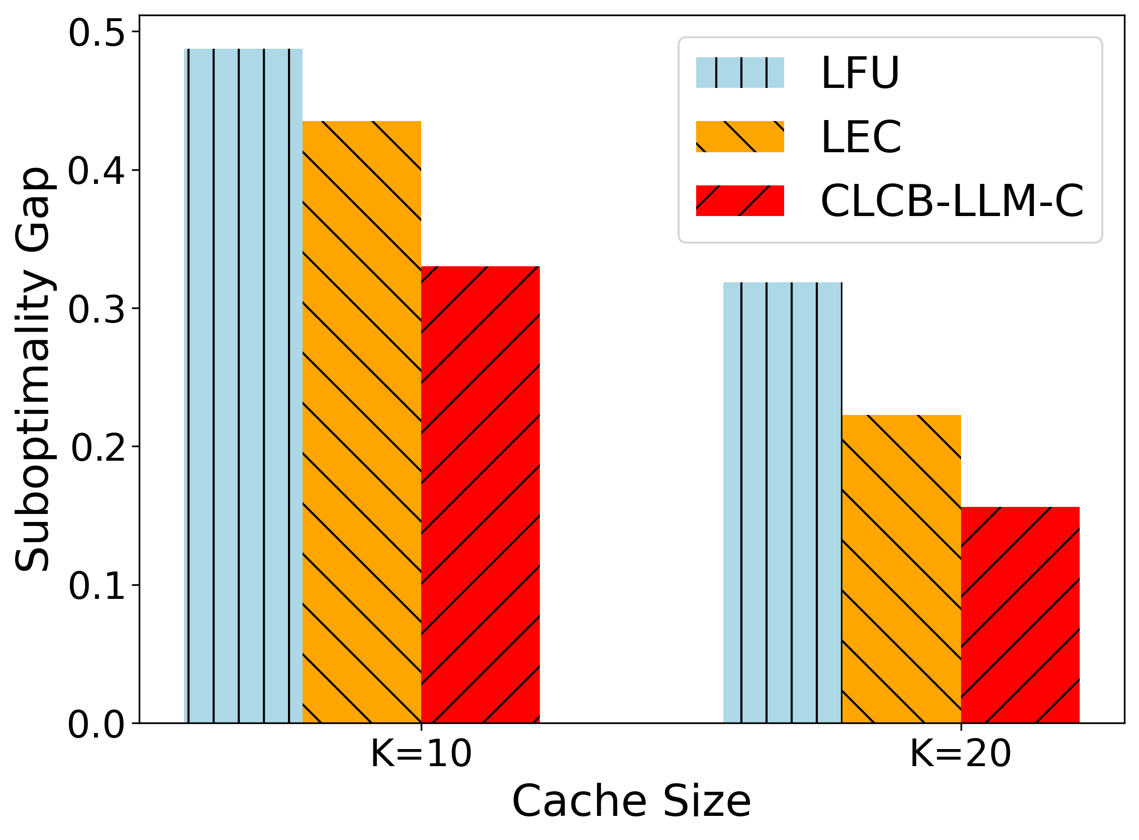
Figure 4: Algorithms on another LLM.

Real-World Dataset. We use the SciQ dataset [120], which covers a variety of topics, including physics, chemistry, and biology, to evaluate the performance of our proposed CLCB-LLM-C algorithm using OpenAI’s LLMs. The cost is defined as the price for API calls, based on OpenAI’s official API pricing. Since the cost heavily depends on the token count of the input text, we utilize OpenAI’s tiktoken library, designed to tokenize text for various GPT models. We consider two different LLMs with distinct encoding strategies. Specifically, we use GPT-4-o with the “o200k_base” encoding to present the main experimental results. Additionally, we experiment with another variant, GPT-4-turbo, which employs the “cl100k_base” encoding [121]. For the evaluation, we work with 100 distinct prompts from the SciQ dataset in an offline setting, performing a total of 10,000 queries with cache sizes of $K=10$ and $K=20$, respectively. Fig. 3(b) presents the normalized suboptimality gap of cost over $n=100$ rounds. CLCB-LLM-C achieves 36.01% and 20.70%, less cost compared to LFU and LEC, respectively. Moreover, a larger $K$ shows a lower suboptimality gap, which is consistent with Theorem˜3. In addition to the results presented in the main text using GPT-4-o with the “o200k_base” encoding, we experiment with another LLM, GPT-4-turbo with the “cl100k_base” encoding. Fig.˜4 demonstrates the robustness of our algorithm across different LLMs.

References

- Cesa-Bianchi and Lugosi [2012] Nicolo Cesa-Bianchi and Gábor Lugosi. Combinatorial bandits. Journal of Computer and System Sciences, 78(5):1404–1422, 2012.
- Bubeck et al. [2012] Sébastien Bubeck, Nicolo Cesa-Bianchi, and Sham M Kakade. Towards minimax policies for online linear optimization with bandit feedback. In Conference on Learning Theory, pages 41–1. JMLR Workshop and Conference Proceedings, 2012.
- Audibert et al. [2014] Jean-Yves Audibert, Sébastien Bubeck, and Gábor Lugosi. Regret in online combinatorial optimization. Mathematics of Operations Research, 39(1):31–45, 2014.
- Neu [2015] Gergely Neu. First-order regret bounds for combinatorial semi-bandits. In Conference on Learning Theory, pages 1360–1375. PMLR, 2015.
- Gai et al. [2012] Yi Gai, Bhaskar Krishnamachari, and Rahul Jain. Combinatorial network optimization with unknown variables: Multi-armed bandits with linear rewards and individual observations. IEEE/ACM Transactions on Networking (TON), 20(5):1466–1478, 2012.
- Kveton et al. [2015a] Branislav Kveton, Zheng Wen, Azin Ashkan, and Csaba Szepesvari. Tight regret bounds for stochastic combinatorial semi-bandits. In AISTATS, 2015a.
- Combes et al. [2015] Richard Combes, Mohammad Sadegh Talebi Mazraeh Shahi, Alexandre Proutiere, et al. Combinatorial bandits revisited. Advances in neural information processing systems, 28, 2015.
- Chen et al. [2016] Wei Chen, Yajun Wang, Yang Yuan, and Qinshi Wang. Combinatorial multi-armed bandit and its extension to probabilistically triggered arms. The Journal of Machine Learning Research, 17(1):1746–1778, 2016.
- Wang and Chen [2017] Qinshi Wang and Wei Chen. Improving regret bounds for combinatorial semi-bandits with probabilistically triggered arms and its applications. In Advances in Neural Information Processing Systems, pages 1161–1171, 2017.
- Merlis and Mannor [2019] Nadav Merlis and Shie Mannor. Batch-size independent regret bounds for the combinatorial multi-armed bandit problem. In Conference on Learning Theory, pages 2465–2489. PMLR, 2019.
- Saha and Gopalan [2019] Aadirupa Saha and Aditya Gopalan. Combinatorial bandits with relative feedback. Advances in Neural Information Processing Systems, 32, 2019.
- Zimmert et al. [2019] Julian Zimmert, Haipeng Luo, and Chen-Yu Wei. Beating stochastic and adversarial semi-bandits optimally and simultaneously. In International Conference on Machine Learning, pages 7683–7692. PMLR, 2019.
- Liu et al. [2024] Xutong Liu, Siwei Wang, Jinhang Zuo, Han Zhong, Xuchuang Wang, Zhiyong Wang, Shuai Li, Mohammad Hajiesmaili, John Lui, and Wei Chen. Combinatorial multivariant multi-armed bandits with applications to episodic reinforcement learning and beyond. arXiv preprint arXiv:2406.01386, 2024.
- Qin et al. [2014] Lijing Qin, Shouyuan Chen, and Xiaoyan Zhu. Contextual combinatorial bandit and its application on diversified online recommendation. In Proceedings of the 2014 SIAM International Conference on Data Mining, pages 461–469. SIAM, 2014.
- Liu et al. [2023a] Xutong Liu, Jinhang Zuo, Siwei Wang, John CS Lui, Mohammad Hajiesmaili, Adam Wierman, and Wei Chen. Contextual combinatorial bandits with probabilistically triggered arms. In International Conference on Machine Learning, pages 22559–22593. PMLR, 2023a.
- Choi et al. [2024] Hyun-jun Choi, Rajan Udwani, and Min-hwan Oh. Cascading contextual assortment bandits. Advances in Neural Information Processing Systems, 36, 2024.
- Hwang et al. [2023] Taehyun Hwang, Kyuwook Chai, and Min-hwan Oh. Combinatorial neural bandits. In International Conference on Machine Learning, pages 14203–14236. PMLR, 2023.
- Kveton et al. [2015b] Branislav Kveton, Csaba Szepesvari, Zheng Wen, and Azin Ashkan. Cascading bandits: Learning to rank in the cascade model. In International Conference on Machine Learning, pages 767–776. PMLR, 2015b.
- Li et al. [2016] Shuai Li, Baoxiang Wang, Shengyu Zhang, and Wei Chen. Contextual combinatorial cascading bandits. In International conference on machine learning, pages 1245–1253. PMLR, 2016.
- Lattimore et al. [2018] Tor Lattimore, Branislav Kveton, Shuai Li, and Csaba Szepesvari. Toprank: A practical algorithm for online stochastic ranking. Advances in Neural Information Processing Systems, 31, 2018.
- Agrawal et al. [2019] Shipra Agrawal, Vashist Avadhanula, Vineet Goyal, and Assaf Zeevi. Mnl-bandit: A dynamic learning approach to assortment selection. Operations Research, 67(5):1453–1485, 2019.
- Lin and Bouneffouf [2022] Baihan Lin and Djallel Bouneffouf. Optimal epidemic control as a contextual combinatorial bandit with budget. In 2022 IEEE International Conference on Fuzzy Systems (FUZZ-IEEE), pages 1–8. IEEE, 2022.
- Verma et al. [2023] Shresth Verma, Aditya Mate, Kai Wang, Neha Madhiwalla, Aparna Hegde, Aparna Taneja, and Milind Tambe. Restless multi-armed bandits for maternal and child health: Results from decision-focused learning. In AAMAS, pages 1312–1320, 2023.
- Bouneffouf et al. [2020] Djallel Bouneffouf, Irina Rish, and Charu Aggarwal. Survey on applications of multi-armed and contextual bandits. In 2020 IEEE Congress on Evolutionary Computation (CEC), pages 1–8. IEEE, 2020.
- György et al. [2007] András György, Tamás Linder, Gábor Lugosi, and György Ottucsák. The on-line shortest path problem under partial monitoring. Journal of Machine Learning Research, 8(10), 2007.
- Kveton et al. [2015c] Branislav Kveton, Zheng Wen, Azin Ashkan, and Csaba Szepesvári. Combinatorial cascading bandits. In Proceedings of the 28th International Conference on Neural Information Processing Systems-Volume 1, pages 1450–1458, 2015c.
- Li et al. [2019] Fengjiao Li, Jia Liu, and Bo Ji. Combinatorial sleeping bandits with fairness constraints. IEEE Transactions on Network Science and Engineering, 7(3):1799–1813, 2019.
- Liu et al. [2023b] Xutong Liu, Jinhang Zuo, Hong Xie, Carlee Joe-Wong, and John CS Lui. Variance-adaptive algorithm for probabilistic maximum coverage bandits with general feedback. In IEEE INFOCOM 2023-IEEE Conference on Computer Communications, pages 1–10. IEEE, 2023b.
- Liu et al. [2022] Xutong Liu, Jinhang Zuo, Siwei Wang, Carlee Joe-Wong, John Lui, and Wei Chen. Batch-size independent regret bounds for combinatorial semi-bandits with probabilistically triggered arms or independent arms. In Advances in Neural Information Processing Systems, 2022.
- Liu et al. [2020] Siqi Liu, Kay Choong See, Kee Yuan Ngiam, Leo Anthony Celi, Xingzhi Sun, and Mengling Feng. Reinforcement learning for clinical decision support in critical care: Comprehensive review. Journal of Medical Internet Research, 22, 2020. URL https://api.semanticscholar.org/CorpusID:219676905.
- Chen et al. [2023] Xiaocong Chen, Siyu Wang, Julian McAuley, D. Jannach, and Lina Yao. On the opportunities and challenges of offline reinforcement learning for recommender systems. ACM Transactions on Information Systems, 2023. URL https://api.semanticscholar.org/CorpusID:261065303.
- Kiran et al. [2020] Bangalore Ravi Kiran, Ibrahim Sobh, Victor Talpaert, Patrick Mannion, Ahmad A. Al Sallab, Senthil Kumar Yogamani, and Patrick P’erez. Deep reinforcement learning for autonomous driving: A survey. IEEE Transactions on Intelligent Transportation Systems, 23:4909–4926, 2020. URL https://api.semanticscholar.org/CorpusID:211011033.
- Liu et al. [2009] Tie-Yan Liu et al. Learning to rank for information retrieval. Foundations and Trends® in Information Retrieval, 3(3):225–331, 2009.
- Zhu et al. [2023] Banghua Zhu, Ying Sheng, Lianmin Zheng, Clark Barrett, Michael Jordan, and Jiantao Jiao. Towards optimal caching and model selection for large model inference. 36:59062–59094, 2023.
- Kempe et al. [2003a] David Kempe, Jon Kleinberg, and Éva Tardos. Maximizing the spread of influence through a social network. In Proceedings of the ninth ACM SIGKDD international conference on Knowledge discovery and data mining, pages 137–146, 2003a.
- Uchiya et al. [2010] Taishi Uchiya, Atsuyoshi Nakamura, and Mineichi Kudo. Algorithms for adversarial bandit problems with multiple plays. In International Conference on Algorithmic Learning Theory, pages 375–389. Springer, 2010.
- Han et al. [2021] Yanjun Han, Yining Wang, and Xi Chen. Adversarial combinatorial bandits with general non-linear reward functions. In International Conference on Machine Learning, pages 4030–4039. PMLR, 2021.
- Ito [2021] Shinji Ito. Hybrid regret bounds for combinatorial semi-bandits and adversarial linear bandits. Advances in Neural Information Processing Systems, 34:2654–2667, 2021.
- Tsuchiya et al. [2023] Taira Tsuchiya, Shinji Ito, and Junya Honda. Further adaptive best-of-both-worlds algorithm for combinatorial semi-bandits. In International Conference on Artificial Intelligence and Statistics, pages 8117–8144. PMLR, 2023.
- Takemura et al. [2021] Kei Takemura, Shinji Ito, Daisuke Hatano, Hanna Sumita, Takuro Fukunaga, Naonori Kakimura, and Ken-ichi Kawarabayashi. Near-optimal regret bounds for xutong combinatorial semi-bandits with linear payoff functions. In Proceedings of the AAAI Conference on Artificial Intelligence, pages 9791–9798, 2021.
- Chen et al. [2018] Lixing Chen, Jie Xu, and Zhuo Lu. Contextual combinatorial multi-armed bandits with volatile arms and submodular reward. Advances in Neural Information Processing Systems, 31, 2018.
- Nika et al. [2020] Andi Nika, Sepehr Elahi, and Cem Tekin. Contextual combinatorial volatile multi-armed bandit with adaptive discretization. In International Conference on Artificial Intelligence and Statistics, pages 1486–1496. PMLR, 2020.
- Ernst et al. [2005] Damien Ernst, Pierre Geurts, and Louis Wehenkel. Tree-based batch mode reinforcement learning. Journal of Machine Learning Research, 6, 2005.
- Riedmiller [2005] Martin Riedmiller. Neural fitted q iteration–first experiences with a data efficient neural reinforcement learning method. In Machine learning: ECML 2005: 16th European conference on machine learning, Porto, Portugal, October 3-7, 2005. proceedings 16, pages 317–328. Springer, 2005.
- Lange et al. [2012] Sascha Lange, Thomas Gabel, and Martin Riedmiller. Batch reinforcement learning. In Reinforcement learning: State-of-the-art, pages 45–73. Springer, 2012.
- Levine et al. [2020] Sergey Levine, Aviral Kumar, George Tucker, and Justin Fu. Offline reinforcement learning: Tutorial, review, and perspectives on open problems. arXiv preprint arXiv:2005.01643, 2020.
- Singh et al. [2021] Bharat Singh, Rajesh Kumar, and Vinay Pratap Singh. Reinforcement learning in robotic applications: a comprehensive survey. Artificial Intelligence Review, 55:945 – 990, 2021. URL https://api.semanticscholar.org/CorpusID:234826156.
- Casper et al. [2023] Stephen Casper, Xander Davies, Claudia Shi, Thomas Krendl Gilbert, J’er’emy Scheurer, Javier Rando, Rachel Freedman, Tomasz Korbak, David Lindner, Pedro Freire, Tony Wang, Samuel Marks, Charbel-Raphaël Ségerie, Micah Carroll, Andi Peng, Phillip J. K. Christoffersen, Mehul Damani, Stewart Slocum, Usman Anwar, Anand Siththaranjan, Max Nadeau, Eric J. Michaud, Jacob Pfau, Dmitrii Krasheninnikov, Xin Chen, Lauro Langosco di Langosco, Peter Hase, Erdem Biyik, Anca D. Dragan, David Krueger, Dorsa Sadigh, and Dylan Hadfield-Menell. Open problems and fundamental limitations of reinforcement learning from human feedback. ArXiv, abs/2307.15217, 2023. URL https://api.semanticscholar.org/CorpusID:260316010.
- Fujimoto et al. [2018] Scott Fujimoto, David Meger, and Doina Precup. Off-policy deep reinforcement learning without exploration. In International Conference on Machine Learning, 2018. URL https://api.semanticscholar.org/CorpusID:54457299.
- Kumar et al. [2019] Aviral Kumar, Justin Fu, G. Tucker, and Sergey Levine. Stabilizing off-policy q-learning via bootstrapping error reduction. In Neural Information Processing Systems, 2019. URL https://api.semanticscholar.org/CorpusID:173990380.
- Haarnoja et al. [2018] Tuomas Haarnoja, Aurick Zhou, P. Abbeel, and Sergey Levine. Soft actor-critic: Off-policy maximum entropy deep reinforcement learning with a stochastic actor. ArXiv, abs/1801.01290, 2018. URL https://api.semanticscholar.org/CorpusID:28202810.
- Kumar et al. [2020] Aviral Kumar, Aurick Zhou, G. Tucker, and Sergey Levine. Conservative q-learning for offline reinforcement learning. ArXiv, abs/2006.04779, 2020. URL https://api.semanticscholar.org/CorpusID:219530894.
- Agarwal et al. [2019] Rishabh Agarwal, Dale Schuurmans, and Mohammad Norouzi. An optimistic perspective on offline reinforcement learning. In International Conference on Machine Learning, 2019. URL https://api.semanticscholar.org/CorpusID:212628904.
- Jiang and Li [2015] Nan Jiang and Lihong Li. Doubly robust off-policy value evaluation for reinforcement learning. In International Conference on Machine Learning, 2015. URL https://api.semanticscholar.org/CorpusID:5806691.
- Nachum et al. [2019] Ofir Nachum, Bo Dai, Ilya Kostrikov, Yinlam Chow, Lihong Li, and Dale Schuurmans. Algaedice: Policy gradient from arbitrary experience. ArXiv, abs/1912.02074, 2019. URL https://api.semanticscholar.org/CorpusID:208617840.
- Fujimoto and Gu [2021] Scott Fujimoto and Shixiang Shane Gu. A minimalist approach to offline reinforcement learning. ArXiv, abs/2106.06860, 2021. URL https://api.semanticscholar.org/CorpusID:235422620.
- Chen et al. [2019] Xinyue Chen, Zijian Zhou, Z. Wang, Che Wang, Yanqiu Wu, Qing Deng, and Keith W. Ross. Bail: Best-action imitation learning for batch deep reinforcement learning. ArXiv, abs/1910.12179, 2019. URL https://api.semanticscholar.org/CorpusID:204907199.
- Kidambi et al. [2020] Rahul Kidambi, Aravind Rajeswaran, Praneeth Netrapalli, and Thorsten Joachims. Morel : Model-based offline reinforcement learning. ArXiv, abs/2005.05951, 2020. URL https://api.semanticscholar.org/CorpusID:218595964.
- Yu et al. [2021] Tianhe Yu, Aviral Kumar, Rafael Rafailov, Aravind Rajeswaran, Sergey Levine, and Chelsea Finn. Combo: Conservative offline model-based policy optimization. In Neural Information Processing Systems, 2021. URL https://api.semanticscholar.org/CorpusID:231934209.
- Szepesvari and Munos [2005] Csaba Szepesvari and Rémi Munos. Finite time bounds for sampling based fitted value iteration. Proceedings of the 22nd international conference on Machine learning, 2005. URL https://api.semanticscholar.org/CorpusID:8617488.
- Chen and Jiang [2019a] Jinglin Chen and Nan Jiang. Information-theoretic considerations in batch reinforcement learning. In International Conference on Machine Learning, 2019a. URL https://api.semanticscholar.org/CorpusID:141460093.
- Wang et al. [2019] Lingxiao Wang, Qi Cai, Zhuoran Yang, and Zhaoran Wang. Neural policy gradient methods: Global optimality and rates of convergence. ArXiv, abs/1909.01150, 2019. URL https://api.semanticscholar.org/CorpusID:202121359.
- Xie et al. [2021a] Tengyang Xie, Ching-An Cheng, Nan Jiang, Paul Mineiro, and Alekh Agarwal. Bellman-consistent pessimism for offline reinforcement learning. In Neural Information Processing Systems, 2021a. URL https://api.semanticscholar.org/CorpusID:235422048.
- Rashidinejad et al. [2021] Paria Rashidinejad, Banghua Zhu, Cong Ma, Jiantao Jiao, and Stuart J. Russell. Bridging offline reinforcement learning and imitation learning: A tale of pessimism. IEEE Transactions on Information Theory, 68:8156–8196, 2021.
- Yin et al. [2021] Ming Yin, Yu Bai, and Yu-Xiang Wang. Near-optimal offline reinforcement learning via double variance reduction. ArXiv, abs/2102.01748, 2021. URL https://api.semanticscholar.org/CorpusID:231786531.
- Shi et al. [2022] Laixi Shi, Gen Li, Yuting Wei, Yuxin Chen, and Yuejie Chi. Pessimistic q-learning for offline reinforcement learning: Towards optimal sample complexity. ArXiv, abs/2202.13890, 2022. URL https://api.semanticscholar.org/CorpusID:247159013.
- Li et al. [2022a] Gen Li, Laixi Shi, Yuxin Chen, Yuejie Chi, and Yuting Wei. Settling the sample complexity of model-based offline reinforcement learning. ArXiv, abs/2204.05275, 2022a. URL https://api.semanticscholar.org/CorpusID:248085509.
- Jin et al. [2020a] Ying Jin, Zhuoran Yang, and Zhaoran Wang. Is pessimism provably efficient for offline rl? In International Conference on Machine Learning, 2020a. URL https://api.semanticscholar.org/CorpusID:229923558.
- Chang et al. [2021] Jonathan D. Chang, Masatoshi Uehara, Dhruv Sreenivas, Rahul Kidambi, and Wen Sun. Mitigating covariate shift in imitation learning via offline data with partial coverage. In Neural Information Processing Systems, 2021. URL https://api.semanticscholar.org/CorpusID:248498378.
- Bai et al. [2022] Chenjia Bai, Lingxiao Wang, Zhuoran Yang, Zhihong Deng, Animesh Garg, Peng Liu, and Zhaoran Wang. Pessimistic bootstrapping for uncertainty-driven offline reinforcement learning, 2022. URL https://arxiv.org/abs/2202.11566.
- Rashidinejad et al. [2022] Paria Rashidinejad, Hanlin Zhu, Kunhe Yang, Stuart J. Russell, and Jiantao Jiao. Optimal conservative offline rl with general function approximation via augmented lagrangian. ArXiv, abs/2211.00716, 2022. URL https://api.semanticscholar.org/CorpusID:253255046.
- Zanette et al. [2021] Andrea Zanette, Martin J Wainwright, and Emma Brunskill. Provable benefits of actor-critic methods for offline reinforcement learning. Advances in neural information processing systems, 34:13626–13640, 2021.
- Xie et al. [2021b] Tengyang Xie, Ching-An Cheng, Nan Jiang, Paul Mineiro, and Alekh Agarwal. Bellman-consistent pessimism for offline reinforcement learning. Advances in neural information processing systems, 34:6683–6694, 2021b.
- Zanette and Wainwright [2022] Andrea Zanette and Martin J Wainwright. Bellman residual orthogonalization for offline reinforcement learning. Advances in Neural Information Processing Systems, 35:3137–3151, 2022.
- Li et al. [2022b] Gene Li, Cong Ma, and Nati Srebro. Pessimism for offline linear contextual bandits using confidence sets. Advances in Neural Information Processing Systems, 35:20974–20987, 2022b.
- Nguyen-Tang et al. [2021a] Thanh Nguyen-Tang, Sunil Gupta, Hung Tran-The, and Svetha Venkatesh. Sample complexity of offline reinforcement learning with deep relu networks. arXiv preprint arXiv:2103.06671, 2021a.
- Nguyen-Tang et al. [2021b] Thanh Nguyen-Tang, Sunil Gupta, A Tuan Nguyen, and Svetha Venkatesh. Offline neural contextual bandits: Pessimism, optimization and generalization. arXiv preprint arXiv:2111.13807, 2021b.
- Wang and Chen [2018] Siwei Wang and Wei Chen. Thompson sampling for combinatorial semi-bandits. In International Conference on Machine Learning, pages 5114–5122, 2018.
- Vial et al. [2022] Daniel Vial, Sanjay Shakkottai, and R Srikant. Minimax regret for cascading bandits. In Advances in Neural Information Processing Systems, 2022.
- Zhong et al. [2021] Zixin Zhong, Wang Chi Chueng, and Vincent YF Tan. Thompson sampling algorithms for cascading bandits. Journal of Machine Learning Research, 22(218):1–66, 2021.
- Wang et al. [2023] Yiliu Wang, Wei Chen, and Milan Vojnović. Combinatorial bandits for maximum value reward function under max value-index feedback. arXiv preprint arXiv:2305.16074, 2023.
- Wang et al. [2024] Dairui Wang, Junyu Cao, Yan Zhang, and Wei Qi. Cascading bandits: optimizing recommendation frequency in delayed feedback environments. Advances in Neural Information Processing Systems, 36, 2024.
- Joachims [2002] Thorsten Joachims. Optimizing search engines using clickthrough data. Proceedings of the eighth ACM SIGKDD international conference on Knowledge discovery and data mining, 2002. URL https://api.semanticscholar.org/CorpusID:207605508.
- Wang et al. [2018] Xuanhui Wang, Nadav Golbandi, Michael Bendersky, Donald Metzler, and Marc Najork. Position bias estimation for unbiased learning to rank in personal search. Proceedings of the Eleventh ACM International Conference on Web Search and Data Mining, 2018. URL https://api.semanticscholar.org/CorpusID:21054674.
- Wang et al. [2016] Xuanhui Wang, Michael Bendersky, Donald Metzler, and Marc Najork. Learning to rank with selection bias in personal search. Proceedings of the 39th International ACM SIGIR conference on Research and Development in Information Retrieval, 2016. URL https://api.semanticscholar.org/CorpusID:15989814.
- Keane and O’Brien [2006] Mark T. Keane and Maeve O’Brien. Modeling result-list searching in the world wide web: The role of relevance topologies and trust bias. 2006. URL https://api.semanticscholar.org/CorpusID:18100844.
- Zhang et al. [2023] Zeyu Zhang, Yi-Hsun Su, Hui Yuan, Yiran Wu, Rishab Balasubramanian, Qingyun Wu, Huazheng Wang, and Mengdi Wang. Unified off-policy learning to rank: a reinforcement learning perspective. ArXiv, abs/2306.07528, 2023. URL https://api.semanticscholar.org/CorpusID:259145065.
- Pope et al. [2022] Reiner Pope, Sholto Douglas, Aakanksha Chowdhery, Jacob Devlin, James Bradbury, Anselm Levskaya, Jonathan Heek, Kefan Xiao, Shivani Agrawal, and Jeff Dean. Efficiently scaling transformer inference. ArXiv, abs/2211.05102, 2022. URL https://api.semanticscholar.org/CorpusID:253420623.
- Kwon et al. [2023] Woosuk Kwon, Zhuohan Li, Siyuan Zhuang, Ying Sheng, Lianmin Zheng, Cody Hao Yu, Joseph E. Gonzalez, Haotong Zhang, and Ion Stoica. Efficient memory management for large language model serving with pagedattention. Proceedings of the 29th Symposium on Operating Systems Principles, 2023. URL https://api.semanticscholar.org/CorpusID:261697361.
- Sheng et al. [2023] Ying Sheng, Lianmin Zheng, Binhang Yuan, Zhuohan Li, Max Ryabinin, Daniel Y. Fu, Zhiqiang Xie, Beidi Chen, Clark W. Barrett, Joseph Gonzalez, Percy Liang, Christopher Ré, Ion Stoica, and Ce Zhang. High-throughput generative inference of large language models with a single gpu. In International Conference on Machine Learning, 2023. URL https://api.semanticscholar.org/CorpusID:257495837.
- Bang [2023] Fu Bang. Gptcache: An open-source semantic cache for llm applications enabling faster answers and cost savings. Proceedings of the 3rd Workshop for Natural Language Processing Open Source Software (NLP-OSS 2023), 2023. URL https://api.semanticscholar.org/CorpusID:265607979.
- Gim et al. [2023] In Gim, Guojun Chen, Seung seob Lee, Nikhil Sarda, Anurag Khandelwal, and Lin Zhong. Prompt cache: Modular attention reuse for low-latency inference. ArXiv, abs/2311.04934, 2023. URL https://api.semanticscholar.org/CorpusID:265067391.
- Qu et al. [2024] Guanqiao Qu, Qiyuan Chen, Wei Wei, Zhengyi Lin, Xianhao Chen, and Kaibin Huang. Mobile edge intelligence for large language models: A contemporary survey. ArXiv, abs/2407.18921, 2024. URL https://api.semanticscholar.org/CorpusID:271534421.
- Dai et al. [2024a] Xiangxiang Dai, Jin Li, Xutong Liu, Anqi Yu, and John C. S. Lui. Cost-effective online multi-llm selection with versatile reward models. ArXiv, abs/2405.16587, 2024a. URL https://api.semanticscholar.org/CorpusID:270063595.
- Feng et al. [2024] Tao Feng, Yanzhen Shen, and Jiaxuan You. Graphrouter: A graph-based router for llm selections. ArXiv, abs/2410.03834, 2024. URL https://api.semanticscholar.org/CorpusID:273185502.
- Richardson and Domingos [2002] Matthew Richardson and Pedro M. Domingos. Mining knowledge-sharing sites for viral marketing. Proceedings of the eighth ACM SIGKDD international conference on Knowledge discovery and data mining, 2002. URL https://api.semanticscholar.org/CorpusID:5785954.
- Kempe et al. [2003b] David Kempe, Jon M. Kleinberg, and Éva Tardos. Maximizing the spread of influence through a social network. Theory Comput., 11:105–147, 2003b. URL https://api.semanticscholar.org/CorpusID:7214363.
- Chen et al. [2009] Wei Chen, Yajun Wang, and Siyu Yang. Efficient influence maximization in social networks. In Knowledge Discovery and Data Mining, 2009. URL https://api.semanticscholar.org/CorpusID:10417256.
- Wen et al. [2017] Zheng Wen, Branislav Kveton, Michal Valko, and Sharan Vaswani. Online influence maximization under independent cascade model with semi-bandit feedback. Advances in neural information processing systems, 30, 2017.
- Vaswani et al. [2017a] Sharan Vaswani, Branislav Kveton, Zheng Wen, Mohammad Ghavamzadeh, Laks Lakshmanan, and Mark Schmidt. Diffusion independent semi-bandit influence maximization. In Proceedings of the 34th International Conference on Machine Learning (ICML), 2017a.
- Wu et al. [2019] Qingyun Wu, Zhige Li, Huazheng Wang, Wei Chen, and Hongning Wang. Factorization bandits for online influence maximization. Proceedings of the 25th ACM SIGKDD International Conference on Knowledge Discovery & Data Mining, 2019. URL https://api.semanticscholar.org/CorpusID:182952558.
- Vaswani et al. [2017b] Sharan Vaswani, Branislav Kveton, Zheng Wen, Mohammad Ghavamzadeh, Laks V. S. Lakshmanan, and Mark W. Schmidt. Model-independent online learning for influence maximization. In International Conference on Machine Learning, 2017b. URL https://api.semanticscholar.org/CorpusID:32455974.
- Vaswani et al. [2015] Sharan Vaswani, Laks Lakshmanan, Mark Schmidt, et al. Influence maximization with bandits. arXiv preprint arXiv:1503.00024, 2015.
- Balkanski et al. [2015] Eric Balkanski, Aviad Rubinstein, and Yaron Singer. The limitations of optimization from samples. Proceedings of the 49th Annual ACM SIGACT Symposium on Theory of Computing, 2015. URL https://api.semanticscholar.org/CorpusID:742580.
- Balkanski et al. [2016] Eric Balkanski, Aviad Rubinstein, and Yaron Singer. The power of optimization from samples. In Neural Information Processing Systems, 2016. URL https://api.semanticscholar.org/CorpusID:15394546.
- Chen et al. [2020] Wei Chen, Xiaoming Sun, Jialin Zhang, and Zhijie Zhang. Optimization from structured samples for coverage functions. In International Conference on Machine Learning, pages 1715–1724. PMLR, 2020.
- Chen et al. [2021] Wei Chen, Xiaoming Sun, Jialin Zhang, and Zhijie Zhang. Network inference and influence maximization from samples. In International Conference on Machine Learning, pages 1707–1716. PMLR, 2021.
- Zuo and Joe-Wong [2021] Jinhang Zuo and Carlee Joe-Wong. Combinatorial multi-armed bandits for resource allocation. In 2021 55th Annual Conference on Information Sciences and Systems (CISS), pages 1–4. IEEE, 2021.
- Chen et al. [2013] Wei Chen, Yajun Wang, and Yang Yuan. Combinatorial multi-armed bandit: General framework and applications. In International Conference on Machine Learning, pages 151–159. PMLR, 2013.
- Chen and Jiang [2019b] Jinglin Chen and Nan Jiang. Information-theoretic considerations in batch reinforcement learning. In International Conference on Machine Learning, pages 1042–1051. PMLR, 2019b.
- Jiang [2019] Nan Jiang. On value functions and the agent-environment boundary. arXiv preprint arXiv:1905.13341, 2019.
- Jin et al. [2020b] Chi Jin, Zhuoran Yang, Zhaoran Wang, and Michael I Jordan. Provably efficient reinforcement learning with linear function approximation. In Conference on Learning Theory, pages 2137–2143. PMLR, 2020b.
- Hu et al. [2018] Yujing Hu, Qing Da, Anxiang Zeng, Yang Yu, and Yinghui Xu. Reinforcement learning to rank in e-commerce search engine: Formalization, analysis, and application. In Proceedings of the 24th ACM SIGKDD international conference on knowledge discovery & data mining, pages 368–377, 2018.
- Karmaker Santu et al. [2017] Shubhra Kanti Karmaker Santu, Parikshit Sondhi, and ChengXiang Zhai. On application of learning to rank for e-commerce search. In Proceedings of the 40th international ACM SIGIR conference on research and development in information retrieval, pages 475–484, 2017.
- Karatzoglou et al. [2013] Alexandros Karatzoglou, Linas Baltrunas, and Yue Shi. Learning to rank for recommender systems. In Proceedings of the 7th ACM Conference on Recommender Systems, pages 493–494, 2013.
- Craswell et al. [2008] Nick Craswell, Onno Zoeter, Michael Taylor, and Bill Ramsey. An experimental comparison of click position-bias models. In Proceedings of the 2008 international conference on web search and data mining, pages 87–94, 2008.
- Chen et al. [2010] Wei Chen, Yifei Yuan, and Li Zhang. Scalable influence maximization in social networks under the linear threshold model. In 2010 IEEE international conference on data mining, pages 88–97. IEEE, 2010.
- Narasimhan et al. [2015] Harikrishna Narasimhan, David C Parkes, and Yaron Singer. Learnability of influence in networks. Advances in Neural Information Processing Systems, 28, 2015.
- Liu et al. [2021] Xutong Liu, Jinhang Zuo, Xiaowei Chen, Wei Chen, and John CS Lui. Multi-layered network exploration via random walks: From offline optimization to online learning. In International Conference on Machine Learning, pages 7057–7066. PMLR, 2021.
- Welbl et al. [2017] Johannes Welbl, Nelson F Liu, and Matt Gardner. Crowdsourcing multiple choice science questions. arXiv preprint arXiv:1707.06209, 2017.
- OpenAI [2025] OpenAI. OpenAI LLM API. https://platform.openai.com/, 2025.
- Le Cam [2012] Lucien Le Cam. Asymptotic methods in statistical decision theory. Springer Science & Business Media, 2012.
- Lattimore and Szepesvári [2020] Tor Lattimore and Csaba Szepesvári. Bandit algorithms. Cambridge University Press, 2020.
- Dai et al. [2024b] Xiangxiang Dai, Zhiyong Wang, Jize Xie, Xutong Liu, and John CS Lui. Conversational recommendation with online learning and clustering on misspecified users. IEEE Transactions on Knowledge and Data Engineering, 36(12):7825–7838, 2024b.