Study on the $P$-wave form factors contributing to $B_{s}$ to $D_{s}$ inclusive semileptonic decays from lattice simulations

Abstract

We present a pilot study on extracting the form factors of the semileptonic decay of a $B_{s}$ meson to the $P$-wave $D_{s}^{**}$ states from $B_{s}$ four-point correlators. With their inclusive nature, four-point correlators include contributions from all possible final states. From the extracted $P$-wave form factors, we obtain numerical results for the corresponding Isgur-Wise form factors. The results suggest significant contributions from radial excitations to the Uraltsev sum rule at zero-recoil. In this pilot study, a coarse lattice of $24^{3}\times 64$ with lattice spacing of $0.11\,\mathrm{fm}$ is used for the analysis.

1 Introduction

Some tensions remain in flavor physics, including the well-known inconsistency between inclusive and exclusive determinations of $|V_{cb}|$ [1]. A less famous example is the puzzle concerning the $B$-meson semileptonic decay rates to excited $D$ mesons. According to heavy quark effective theory (HQET), the branching ratio of $B_{(s)}$ decaying into the $P_{3/2}$-channel $D_{(s)}$ mesons should be much larger than that to the $P_{1/2}$-channel $D_{(s)}$ mesons, but it contradicts the experimental data of the $B$ decays. It is called the 1/2-versus-3/2 puzzle [2]. This may be the source of another problem in the semileptonic $B$ decays, i.e. the gap between the sum of currently observed exclusive branching ratios of the $b\rightarrow c$ semileptonic decays and the corresponding inclusive decay width.

The connection between inclusive and exclusive observables may be established through the four-point correlators on the lattice [3, 4]. This work presents a pilot study to extract exclusive information from the four-point correlators of the $B_{s}$ meson calculated on the lattice. In Sec. 2 we present the four-point correlator $C_{J_{\mu}J_{\nu}}$ and its relation to inclusive and exclusive processes. In Sec. 3, we decompose $C_{J_{\mu}J_{\nu}}$ using the exclusive form factors. In Sec. 4 we introduce the lattice setup and Sec. 5 contains our numerical results. We conclude this paper with discussions in Sec. 6.

2 Semileptonic decays and $C_{J_{\mu}J_{\nu}}$

We begin by elucidating the kinematics of the $B_{s}$ semileptonic decays $B_{s}\longrightarrow{X_{cs}}l\nu_{l}$. We work in the center-of-mass frame of the ${B_{s}}$ meson, i.e., $p_{B_{s}}=(M_{B_{s}},\boldsymbol{0})$. The momentum carried away by the lepton pair is $q=p_{B_{s}}-p_{{X_{cs}}}=(M_{B_{s}}-E_{X_{cs}},\boldsymbol{q})$, where $E_{X_{cs}}$ is the energy left for the final-state hadron.

For the inclusive semileptonic decays, the differential cross section after angular and lepton energy integrals reads

$$\frac{\mathrm{d}\Gamma^{\mathrm{inc}}}{\mathrm{d}\boldsymbol{q}^{2}}\propto G_{F}^{2}\absolutevalue{V_{cb}}^{2}\int\mathrm{d}E_{X_{cs}}\,W^{\mu\nu}(\boldsymbol{q},E_{X_{cs}})k_{\mu\nu}(\boldsymbol{q},E_{X_{cs}})\,,$$ (1)

where $k_{\mu\nu}$ is a known kinematic factor, $G_{F}$ is the Fermi constant, and $V_{cb}$ is the CKM matrix element related to the flavor-changing process $b\rightarrow c$. The strong-interaction dynamics is encoded in the forward hadronic tensor $W^{\mu\nu}$.

Through a Laplace transform, $W^{\mu\nu}$ is related to a quantity that is accessible in lattice simulations:

$$\scriptstyle C_{J_{\mu}J_{\nu}}(\boldsymbol{q},t)\equiv\int\mathrm{d}^{3}\boldsymbol{x}\frac{e^{i\boldsymbol{q}\cdot\boldsymbol{x}}}{2M_{B_{s}}}\Braket{B_{s}|J_{\mu}^{\dagger}(\boldsymbol{x},0)e^{-\hat{H}t}J_{\nu}(0)|B_{s}}=\int_{0}^{\infty}\mathrm{d}E_{X_{cs}}e^{-tE_{X_{cs}}}W^{\mu\nu}(\boldsymbol{q},E_{X_{cs}})\,.$$ (2)

Inverting the Laplace transform to obtain the hadronic tensor from the lattice data is an ill-posed inverse problem. But for inclusive decays, what is most important is not $W^{\mu\nu}$ itself, but its weighted integral over $E_{X_{cs}}$. Thus, expressing $k_{\mu\nu}$ by polynomials of $\exp(-E_{X_{cs}})$, we can avoid this inverse problem to obtain estimates of the inclusive observables from $C_{J_{\mu}J_{\nu}}(\boldsymbol{q},t)$. See [4, 5, 6, 7, 8] for more details on the inclusive calculations.

On the other hand, the exclusive differential decay rate generally takes the following form

$$\frac{\mathrm{d}\Gamma^{\mathrm{exc}}}{\mathrm{d}w}\propto G_{F}^{2}\left|V_{cb}\right|^{2}H\left(\mathcal{F}(w),\mathcal{K}(w,M_{{X_{cs}}})\right)\,.$$ (3)

Here, $\mathcal{F}(w)$’s are form factors to parameterize the relevant hadronic transition matrix elements; $\mathcal{K}(w,M_{{X_{cs}}})$’s are known kinematical factors and $H$ represents a collection of them. For exclusive processes, we introduce the recoil parameter $w\equiv v^{\prime}\cdot v$, with $v$ and $v^{\prime}$ the four-velocity of $B_{s}$ and ${X_{cs}}$ respectively, and thus $w=\sqrt{1+\boldsymbol{q}^{2}/M_{{X_{cs}}}^{2}}$.

Usually, the non-perturbative form factors $\mathcal{F}(w)$ are extracted from large time-separations of Euclidean three-point correlators, and only the ground-state (thus exclusive) form factors are obtained with meaningful precision. Here, we propose to extract them, along with the mass spectrum of the final states, from $C_{J_{\mu}J_{\nu}}(\boldsymbol{q},t)$, which contains contributions from all possible final states. We notice that by inserting a complete set of final states, $C_{J_{\mu}J_{\nu}}(\boldsymbol{q},t)$ becomes the sum of a series of exponentials

$$C_{J_{\mu}J_{\nu}}(\boldsymbol{q},t)=\sum_{X_{cs}}\int\!\frac{d^{3}\boldsymbol{p}_{X_{cs}}}{4E_{X_{cs}}M_{B_{s}}}\delta^{(3)}(\boldsymbol{q}+\boldsymbol{p}_{X_{cs}})\Braket{B_{s}|J^{\dagger}_{\mu}(0)|X_{cs}}\Braket{X_{cs}|J_{\nu}(0)|B_{s}}e^{-E_{X_{cs}}t}\,.$$ (4)

The prefactor of every exponential is nothing but the corresponding hadronic transition matrix element, which in turn is parameterized by form factors $\mathcal{F}(w)$. Thus, we can in principle obtain exclusive information by performing a multiple-exponential fit of $C_{J_{\mu}J_{\nu}}(\boldsymbol{q},t)$.

From Eq. (2) and Eq. (4), it is clear that inclusive and exclusive differential decay rates are related to the same quantity $C_{J_{\mu}J_{\nu}}(\boldsymbol{q},t)$. In this way, the saturation of the inclusive decay rate by exclusive channels should naturally be satisfied. This may provide a way to understand the tensions mentioned above, once precisely calculated on the lattice. Further, we also aspire to explore a new possibility to extract transition form factors into orbitally excited final states from lattice simulations with finite heavy-quark masses. Preliminary investigations, like that in Ref. [9], via three-point correlators are heavily obstructed by the complexity of constructing proper interpolating operators and the large noise.

3 Decompositions of $C_{J_{\mu}J_{\nu}}$ into different final states

Heavy-quark symmetry provides a baseline understanding of the spectrum and transition of heavy mesons. In the $m_{b},m_{c}\rightarrow\infty$ limit, the spectrum of the heavy-light mesons can be classified by the radial excitation and the total angular momentum of the light degrees of freedom. For each of the radial excitations, degenerate pairs can be found with the same total angular momentum and parity of the light degrees of freedom $j^{\mathcal{P}}$. Here, we focus on the radial ground states of the $D_{s}$ mesons. By coupling $j^{\mathcal{P}}=(1/2)^{-}$ with the spin of the heavy quark $s_{c}=1/2$, we obtain the $S$-wave pair $J^{\mathcal{P}}=(0^{-},1^{-})$, i.e., $D_{s}$ and $D_{s}^{*}$. The four lightest positive-parity states can also be classified into the $P_{1/2}$ ($j^{\mathcal{P}}=(1/2)^{+}$) pair $J^{\mathcal{P}}=(0^{+},1^{+})$, i.e., $D_{s0}^{*}$ and $D_{s1}^{\prime}$, and the $P_{3/2}$ ($j^{\mathcal{P}}=(3/2)^{+}$) pair $J^{\mathcal{P}}=(1^{+},2^{+})$, i.e., $D_{s1}$ and $D_{s2}$. The mass splitting within each pair is proportional to $1/m_{Q}$ and thus vanishes in the heavy-quark limit.

At the zeroth order of HQET, the transitions from the $B_{s}$ to the $D_{s}$ mesons are described by three sets of form factors $\xi^{(n)}(w)$, $\tau_{1/2}^{(n)}(w)$ and $\tau_{3/2}^{(n)}(w)$ for $S$, $P_{1/2}$ and $P_{3/2}$ channels, respectively [10, 11]. Uraltsev proposed a sum rule among the $P$-wave form factors [12]

$$\scriptstyle\sum_{n}\left(\left|\tau_{3/2}^{(n)}(1)\right|^{2}-\left|\tau_{1/2}^{(n)}(1)\right|^{2}\right)=\frac{1}{4}\,.$$ (5)

Here $n$ is the quantum number of radial excitation. Naively, one expects the saturation of this sum rule from the radial ground state, i.e., $\tau_{1/2}=\tau_{1/2}^{(0)}$ and $\tau_{3/2}=\tau_{3/2}^{(0)}$, which suggests $\tau_{3/2}(1)\gg\tau_{1/2}(1)$. This leads to the prediction that the branching ratios for the $(1/2)^{+}$ pairs should be suppressed compared to those of the $(3/2)^{+}$ pairs under the assumption that the form factors depend only mildly on $w$. This assumption should be verified by explicit numerical calculations.

Away from the heavy-quark limit, there are the following form factors to parameterize the semileptonic transitions of $B_{s}$. For $S$-channel ($j^{\mathcal{P}}=(1/2)^{-}$) final states, we have

$$\scriptstyle\Braket{B_{s},v|V_{\mu}|D_{s},v^{\prime}} =\left[h_{+}(v_{\mu}+v^{\prime}_{\mu})+{h_{-}(v_{\mu}-v^{\prime}_{\mu})}\right]\sqrt{M_{B_{s}}M_{D_{s}}}\,,$$ (6)

$$\scriptstyle\Braket{B_{s},v|V_{\mu}|D^{*}_{s},v^{\prime},\epsilon} =\left[{h_{V}\varepsilon_{\mu\alpha\beta\gamma}\epsilon^{\alpha}v^{\prime,\beta}v^{\gamma}}\right]\sqrt{M_{B_{s}}M_{D^{*}_{s}}}\,,$$ (7)

$$\scriptstyle\Braket{B_{s},v|A_{\mu}|D^{*}_{s},v^{\prime},\epsilon} =i\left[(w+1)h_{A1}\epsilon_{\mu}-{(\epsilon\cdot v)\left(h_{A2}v_{\mu}+h_{A3}v^{\prime}_{\mu}\right)}\right]\sqrt{M_{B_{s}}M_{D^{*}_{s}}}\,.$$ (8)

For $P_{1/2}$-channel ($j^{\mathcal{P}}=(1/2)^{+}$) final states, we have

$$\scriptstyle\Braket{B_{s},v|A_{\mu}|D_{s0}^{*},v^{\prime}} =\left[g_{+}(v_{\mu}+v^{\prime}_{\mu})+{g_{-}(v_{\mu}-v^{\prime}_{\mu})}\right]\sqrt{M_{B}M_{D_{s0}^{*}}}\,.$$ (9)

For $P_{3/2}$-channel ($j^{\mathcal{P}}=(3/2)^{+}$) final states, we have

$$\scriptstyle\Braket{B_{s},v|V_{\mu}|D_{s1},v^{\prime},\epsilon} =\left[f_{V1}\epsilon_{\mu}+{(\epsilon\cdot v)\left(f_{V2}v_{\mu}+f_{V3}v^{\prime}_{\mu}\right)}\right]\sqrt{M_{B_{s}}M_{D_{s1}}}\,,$$ (10)

$$\scriptstyle\Braket{B_{s},v|A_{\mu}|D_{s1},v^{\prime},\epsilon} =-i\left[{f_{A}\varepsilon_{\mu\alpha\beta\gamma}\epsilon^{\alpha}v^{\prime,\beta}v^{\gamma}}\right]\sqrt{M_{B_{s}}M_{D_{s1}}}\,.$$ (11)

Here, $\epsilon$ is the polarization vector for the spin-1 particle. $\Braket{B_{s},v|A_{\mu}|D_{s},v^{\prime}}$ and $\Braket{B_{s},v|V_{\mu}|D_{s0}^{*},v^{\prime}}$ vanish due to conservation of parity. All form factors $h,g,f$ depend only on $w$.

Due to limitations in the signal, we can only identify at most two exponentials from every $C_{J_{\mu}J_{\nu}}(\boldsymbol{q},t)$, which leads us to temporarily ignore the contributions from the highest spin state, i.e. $D_{s2}$. The vector final state in the $P_{1/2}$-channel is also connected to four form factors $g_{V1},g_{V2},g_{V3}$ and $g_{A}$, but numerically they are around one order of magnitude smaller than the corresponding ones from the $P_{3/2}$-channel (see discussions in Sec. 5).

By substituting Eqs. (6–11) into Eq. (4), we obtain the decompositions of $C_{J_{\mu}J_{\nu}}(\boldsymbol{q},t)$ into a series of exponentials with their prefactors given by the corresponding form factors. We summarize the form-factor correspondence of $C_{J_{\mu}J_{\nu}}(\boldsymbol{q},t)$ in Tab. 1. In this table, $\perp$ and $\parallel$ refer to the directions perpendicular and parallel to the three-momentum $\boldsymbol{q}$ and empty cells indicate that the $C_{J_{\mu}J_{\nu}}(\boldsymbol{q},t)$ in this row receives no contributions from the final state in this column.

	$S$-channel		$P_{1/2}$-channel	$P_{3/2}$-channel
	$D_{s}(0^{-})$	$D_{s}^{*}(1^{-})$	$D_{s0}^{*}(0^{+})$	$D_{s1}(1^{+})$
$C_{V_{0}V_{0}}$	$h_{+},h_{-}$			$f_{V1},f_{V2},f_{V3}$
$C_{V_{\parallel}V_{\parallel}}$	$h_{+},h_{-}$			$f_{V1},f_{V3}$
$C_{V_{\perp}V_{\perp}}$		$h_{V}$		$f_{V1}$
$C_{V_{0}V_{\parallel}}$	$h_{+},h_{-}$			$f_{V1},f_{V2},f_{V3}$
$C_{A_{0}A_{0}}$		$h_{A1},h_{A2},h_{A3}$	$g_{+},g_{-}$
$C_{A_{\parallel}A_{\parallel}}$		$h_{A1},h_{A3}$	$g_{+},g_{-}$
$C_{A_{\perp}A_{\perp}}$		$h_{A1}$		$f_{A}$
$C_{A_{0}A_{\parallel}}$		$h_{A1},h_{A2},h_{A3}$	$g_{+},g_{-}$

Table 1: The dependence of $C_{J_{\mu}J_{\nu}}(\boldsymbol{q},t)$ on the form factors defined in Eqs. (6~11).

4 Lattice setup

In this study, we use a $24^{3}\times 64$ lattice from RBC/UKQCD Collaboration with lattice spacing $a^{-1}\approx 1.785\,\mathrm{GeV}$ [13]. We use DWF [14, 15], Möbius DWF [16, 17] and relativistic-heavy-quark action [18, 19] for the valence $s$, $c$, $b$ quarks respectively. Their masses are tuned such that the corresponding $D_{s}$ and $B_{s}$ have masses close to the physical ones. More details about the simulation can be found in Ref. [7] and references therein.

We start with the four-point correlators

$$C^{SJ_{\mu}J_{\nu}S}(t_{\mathrm{snk}},t_{2},t_{1},t_{\mathrm{src}},\boldsymbol{q})\propto\int\mathrm{d}^{3}\boldsymbol{x}\;e^{i\boldsymbol{q}\cdot\boldsymbol{x}}\Braket{0|\phi_{B_{s}}^{S}({t_{\mathrm{snk}}})J^{\dagger}_{\mu}(\boldsymbol{x},t_{2})J_{\nu}(\boldsymbol{0},t_{1})\phi_{B_{s}}^{S\,\dagger}({t_{\mathrm{src}}})|0}\,.$$ (12)

$C_{J_{\mu}J_{\nu}}(\boldsymbol{q},t)$ can then be obtained by taking the ratios between four-point correlators and two-point correlators

$$C_{J_{\mu}J_{\nu}}(\boldsymbol{q},t=t_{2}-t_{1})\propto\frac{C^{SJ_{\mu}J_{\nu}S}(t_{\mathrm{snk}},t_{2},t_{1},t_{\mathrm{src}},\boldsymbol{q})}{C^{SL}(t_{\mathrm{snk}},t_{2})C^{LS}(t_{1},t_{\mathrm{src}})}\,.$$ (13)

In this study, we fix $t_{\mathrm{snk}}-t_{\mathrm{src}}=20$, $t_{2}-t_{\mathrm{src}}=14$ and vary $t_{1}$ from 0 to 14. $L(S)$’s in Eqs. (12, 13) represent local (smearing) interpolating operators of $B_{s}$.

5 Numerical results

In the zero-recoil limit, only four correlators, $C_{V_{0}V_{0}}$, $C_{A_{\parallel}A_{\parallel}}$, $C_{A_{0}A_{0}}$ and $C_{V_{\parallel}V_{\parallel}}$ survive. Furthermore, due to parity conservation, contributions from different $J^{\mathcal{P}}$ channels decouple from each other. Thus, at $w=1$, we have

$$\scriptstyle C_{V_{0}V_{0}}(t) =e^{-E_{D_{s}}t}\left|h_{+}(1)\right|^{2}\,,$$ (14)

$$\scriptstyle C_{A_{\parallel}A_{\parallel}}(t) =e^{-E_{D_{s}^{*}}t}\left|h_{A1}(1)\right|^{2}\,,$$ (15)

$$\scriptstyle C_{A_{0}A_{0}}(t) =e^{-E_{D_{s0}^{*}}t}\left|g_{+}(1)\right|^{2}\,,$$ (16)

$$\scriptstyle C_{V_{\parallel}V_{\parallel}}(t) =e^{-E_{D_{s1}^{\prime}}t}\left|\frac{g_{V1}(1)}{2}\right|^{2}+e^{-E_{D_{s1}}t}\left|\frac{f_{V1}(1)}{2}\right|^{2}\approx e^{-E_{D_{s1}}t}\left|\frac{f_{V1}(1)}{2}\right|^{2}\,,$$ (17)

and all other $C_{J_{\mu}J_{\nu}}(t)$ are zero. In Eq. (17), we neglect the contribution from $\left|g_{V1}(1)\right|^{2}$ because by expanding them to the first order in the HQET [10], we have $g_{V1}(1)\propto\left(\epsilon_{c}-3\epsilon_{b}\right)$ and $f_{V1}(1)\propto\epsilon_{c}$. Here $\epsilon_{c}\equiv 1/2m_{c}$ and $\epsilon_{b}\equiv 1/2m_{b}$. The factor $\left(\epsilon_{c}-3\epsilon_{b}\right)$ is numerically much smaller than $\epsilon_{c}$.

In Fig. 1, we show the results of the single-exponential fit for these four correlators (left panel). From the comparison of the correlators, we find that $C_{V_{0}V_{0}}$ and $C_{A_{\parallel}A_{\parallel}}$, which correspond to the $S$-wave states $D_{s}$ and $D_{s}^{*}$, show much stronger and cleaner signals than $C_{A_{0}A_{0}}$ and $C_{V_{\parallel}V_{\parallel}}$. However, information about the $P$-wave states $D_{s0}^{*}$ and $D_{s1}$ can still be extracted from the last two correlators. The mass hierarchy of those four states can be read from the comparisons of effective masses (right panel). Converting to physical units, we obtain $M_{D_{s}^{*}}-M_{D_{s}}=166.2\pm 4.9\,\mathrm{MeV}$, $M_{D_{s0}^{*}}-M_{D_{s}}=420\pm 160\,\mathrm{MeV}$ and $M_{D_{s1}}-M_{D_{s}}=613\pm 85\,\mathrm{MeV}$. Those values are consistent with PDG [20] within errors.

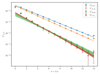
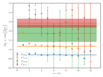
Figure 1: Single-exponential fit of the four non-vanishing correlators at the zero-recoil limit. In the left panel, we compare the fitted (straight lines with errors as bands) and the original (data points) correlators. In the right panel, the effective masses (disconnected points) and the extracted mass parameters (horizontal lines with errors as bands) are plotted together.

Now, let us turn our attention to the form factors. From HQET expanded to the first order in $1/m_{Q}$, the form factors of the $S$-wave final states at the zero-recoil limit are predicted to be

$$h_{+}(1)\approx h_{A1}(1)\approx\xi(1)=1\,.$$ (18)

We obtain $h_{+}(1)=1.004\pm 0.021$ and $h_{A1}(1)=0.885\pm 0.022$, which implies significant (~$10\%$) contributions from the higher orders for $D_{s}^{*}$ and less than a percent contribution for $D_{s}$. The higher order correction to $B_{s}\to D_{s}$ has the form $(\epsilon_{c}-\epsilon_{b})^{2}$ while three separate combinations, $\epsilon_{c}^{2}$, $\epsilon_{c}\epsilon_{b}$, $\epsilon_{b}^{2}$, all appear for $B_{s}\to D_{s}^{*}$, signifying smaller higher order correction for $h_{+}(1)$. The results are also consistent with previous results summarized in FLAG 2024 [21].

For the $P$-wave final states at the zero-recoil limit $w=1$, we obtain $\left|g_{+}(1)\right|=0.166\pm 0.049$ and $\left|f_{V1}(1)\right|=0.445\pm 0.055$ from the lattice data. They are related to the Isgur-Wise form factors as

$$g_{+}(1)\approx-3(\epsilon_{c}+\epsilon_{b})\left(\overline{\Lambda^{*}_{s}}-\overline{\Lambda_{s}}\right)\tau_{1/2}(1)\,,$$ (19)

$$f_{V1}(1)\approx-4\sqrt{2}\epsilon_{c}\left(\overline{\Lambda^{\prime}_{s}}-\overline{\Lambda_{s}}\right)\tau_{3/2}(1)\,.$$ (20)

To obtain an estimate for $\tau_{1/2}(1)$ and $\tau_{3/2}(1)$, we assume nominal values for the mass splittings among $S$, $P_{1/2}$ and $P_{3/2}$ states in the $m_{Q}\rightarrow\infty$ limit, $\left(\overline{\Lambda^{*}_{s}}-\overline{\Lambda_{s}}\right)=0.28\,\mathrm{GeV}$ and $\left(\overline{\Lambda^{\prime}_{s}}-\overline{\Lambda_{s}}\right)=0.41\,\mathrm{GeV}$, from a phenomenological analysis [22]. The quark masses to determine $\epsilon_{b}$ and $\epsilon_{c}$ are $m_{b}=4.8\,\mathrm{GeV}$ and $m_{c}=1.1\,\mathrm{GeV}$. We use a slightly smaller charm-quark mass compared to the phenomenological value [22] in order to accommodate the lighter charm-quark mass in our lattice simulation. Our results are $\left|\tau_{1/2}(1)\right|=0.35\pm 0.10$ and $\left|\tau_{3/2}(1)\right|=0.423\pm 0.052$.

At zero-recoil, form factor $g_{V1}$ can also be expressed as

$$g_{V1}(1)\approx 2\left(\epsilon_{c}-3\epsilon_{b}\right)\left(\overline{\Lambda^{*}_{s}}-\overline{\Lambda_{s}}\right)\tau_{1/2}(1)\,.$$ (21)

Using the value of $\left|\tau_{1/2}(1)\right|$, we obtain $\left|g_{V1}(1)\right|=0.0282\pm 0.083\ll\left|f_{V1}(1)\right|$, validating our choice to ignore the contribution of $D_{s1}^{\prime}$ in Eq. (17). We expect that this suppression is also valid at non-zero recoil, and thus also neglect the contributions from $D_{s1}^{\prime}$ when $\boldsymbol{q}\neq\boldsymbol{0}$ (see Tab. 1).

Moreover, we find $\left(\tau_{3/2}(1)\right)^{2}-\left(\tau_{1/2}(1)\right)^{2}=0.053\pm 0.079$. The deficit compared to 1/4, see Eq. (5), may suggest significant contributions from the radial excitations. We notice, however, that the present study is performed using only one lattice ensemble with limited statistics, and the proper physical limits are still to be taken.

Finally we turn to the analysis at non-zero recoil. We perform multi-exponential fits for $C_{J_{\mu}J_{\nu}}(t)$’s at non-zero $\boldsymbol{q}$. After some simplifications, every four-point correlator is described by the summation of two exponentials with prefactors corresponding to the form factors (see Tab. 1)

$$C_{J_{\mu}J_{\nu}}(t)=\mathcal{A}_{J_{\mu}J_{\nu}}^{\mathrm{GS}}e^{-E_{J_{\mu}J_{\nu}}^{\mathrm{GS}}t}+\mathcal{A}_{J_{\mu}J_{\nu}}^{\mathrm{EX1}}e^{-E_{J_{\mu}J_{\nu}}^{\mathrm{EX1}}t}\,.$$ (22)

Here, $\mathrm{GS}$ stands for ground state and $\mathrm{EX1}$ stands for first excited state. Some of the $C_{J_{\mu}J_{\nu}}(t)$’s receive contributions from the same set of final states, and we perform simultaneous fits of them. We find that for both the ground state and the first excited state contributions, the equality $\mathcal{A}_{V_{0}V_{\parallel}}=\sqrt{\mathcal{A}_{V_{0}V_{0}}\times\mathcal{A}_{V_{\parallel}V_{\parallel}}}$ holds. A similar relation can also be found for the prefactors of $C_{A_{0}A_{0}}$, $C_{A_{\parallel}A_{\parallel}}$ and $C_{A_{0}A_{\parallel}}$. We impose such equalities in our fits, and we introduce the lattice dispersion relation $E=\cosh^{-1}\left[\cosh M+\sum_{i}\left(1-\cos p_{i}\right)\right]$ with the mass values obtained from the zero-recoil analysis to constrain the first exited state energy in Eq. (22). From this fit, we could simultaneously obtain the contributions from both the $S$-channel final states and $P$-channel final states. But here we focus on the $P$-channel results.

We follow the approximation A used in Refs. [22, 10] to express $\mathcal{A}_{V_{0}V_{0}}^{D_{s1}}$ and $\mathcal{A}_{V_{\parallel}V_{\parallel}}^{D_{s1}}$ (we stress that $\mathcal{A}_{V_{0}V_{\parallel}}^{D_{s1}}$ is not a free parameter in our analysis due to the equality) using the zero-recoil values of the Isgur-Wise form factors $\tau(w)\equiv\sqrt{3}\tau_{3/2}(w)$ and its first derivative $\tau(w)=\tau_{0}+\tau^{\prime}(w-1)+\dots$ as

$$\mathcal{A}_{V_{0}V_{0}}^{D_{s1}} \approx\frac{1}{4w}\left\{(w-1)\frac{16}{3}\left[1+2\epsilon_{c}\left(\overline{\Lambda^{\prime}}-\overline{\Lambda}\right)\right]+8(w-1)^{2}\right\}\left(\tau_{0}\right)^{2}+(w-1)^{2}\frac{8\tau_{0}}{3w}\tau^{\prime}\,,$$ (23)

$$\mathcal{A}_{V_{\parallel}V_{\parallel}}^{D_{s1}} \approx\frac{1}{4w}\frac{8}{3}\left[2\left(\overline{\Lambda^{\prime}}-\overline{\Lambda}\right)\epsilon_{c}+(w-1)\right]^{2}\left(\tau_{0}\right)^{2}\,.$$ (24)

Similarly, the contributions from $D_{s0}^{*}$ to $C_{A_{0}A_{0}}$ and $C_{A_{\parallel}A_{\parallel}}$ can also be approximated using the zero-recoil values of the Isgur-Wise form factors $\zeta(w)\equiv 2\tau_{1/2}(w)$ and its first derivative $\zeta(w)=\zeta_{0}+\zeta^{\prime}(w-1)+\dots$ as

$$\mathcal{A}_{A_{0}A_{0}}^{D_{s0}^{*}} \approx\frac{1}{4w}\left[3\left(\overline{\Lambda^{*}}-\overline{\Lambda}\right)(\epsilon_{c}+\epsilon_{b})+(w-1)\right]^{2}\left(\zeta_{0}\right)^{2}\,,$$ (25)

$$\mathcal{A}_{A_{\parallel}A_{\parallel}}^{D_{s0}^{*}} \approx\frac{1}{4w}\left\{2(w-1)\left[1+3(\epsilon_{c}+\epsilon_{b})\left(\overline{\Lambda^{*}}-\overline{\Lambda}\right)\right]+(w-1)^{2}\right\}\left(\zeta_{0}\right)^{2}+(w-1)^{2}\frac{\zeta_{0}}{w}\zeta^{\prime}\,.$$ (26)

The basic idea of approximation A is to treat $w-1$ as the same order as $1/m_{Q}$ and retain only the second order in $\mathcal{O}(w-1)\sim\mathcal{O}(1/m_{Q})$. Thus, Eqs. (23~26) should only be valid at small $\boldsymbol{q}^{2}$, or at $w$ close to $1$.

From the analysis of the correlators at zero recoil, we have $\tau_{0}=\sqrt{3}\tau_{3/2}(1)=0.73\pm 0.09$ and $\zeta_{0}=2\tau_{1/2}(1)=0.71\pm 0.21$, consistent with the phenomenological analysis from Ref. [22]. Thus, Eqs. (24, 25) can be used to check the validity of the approximation A and from Eqs. (23, 26) we may extract the value of $\tau^{\prime}$ and $\zeta^{\prime}$. In Fig. 2, we plot the comparison between those four prefactors extracted from our fits to $C_{J_{\mu}J_{\nu}}$’s and the predictions from approximation A while setting $\tau^{\prime}$ and $\zeta^{\prime}$ to zero in Eqs. (23, 26). Consistency for $\mathcal{A}_{V_{\parallel}V_{\parallel}}^{D_{s1}}$ and $\mathcal{A}_{A_{0}A_{0}}^{D_{s0}^{*}}$ can be readily observed at the smallest non-zero momentum while discrepancy increases with larger $\boldsymbol{q}^{2}$. Thus, we consider it to be safer to extract $\tau^{\prime}$ and $\zeta^{\prime}$ only from the results at the smallest non-zero $\boldsymbol{q}^{2}$. However, it can be observed that this is difficult since the extracted prefactors $\mathcal{A}_{V_{0}V_{0}}^{D_{s1}}$ and $\mathcal{A}_{A_{\parallel}A_{\parallel}}^{D_{s0}^{*}}$ are dominated by error. Indeed, we obtain $\tau^{\prime}=-1\pm 17$ and $\zeta^{\prime}=-18\pm 10$. Such large errors prevent us from drawing any decisive conclusion. Closer investigations are demanded using finer lattice simulations and with better statistics.

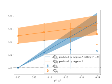
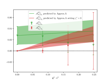
Figure 2: Four prefactors $\mathcal{A}_{V_{0}V_{0}}^{D_{s1}}$, $\mathcal{A}_{V_{\parallel}V_{\parallel}}^{D_{s1}}$, $\mathcal{A}_{A_{0}A_{0}}^{D_{s0}^{*}}$, $\mathcal{A}_{A_{\parallel}A_{\parallel}}^{D_{s9}^{*}}$ extracted from our fitting (data points) and those predicted by approximation A (Eqs. (23~26), bands).

6 Discussions

This work represents a pilot study of extracting information about the $B_{(s)}\rightarrow D_{(s)}$ exclusive decays from the lattice four-point correlators $C_{J_{\mu}J_{\nu}}$. Our motivation is closely connected to the recent effort [8, 5, 6, 7] to extract inclusive decay width also from $C_{J_{\mu}J_{\nu}}$. By performing those two calculations based on the same set of lattice correlators, we open the possibility of simultaneous extractions of $V_{cb}$, and may alleviate the current tension about this CKM matrix element. However, this research requires careful multi-exponential fits of the lattice data and may demand larger source-sink separation and better statistics than that currently used to secure the extraction of excited-state contributions at non-zero recoil.

References

- [1] HFLAV collaboration, Averages of b-hadron, c-hadron, and -lepton properties as of 2021, Phys. Rev. D 107 (2023) 052008 [2206.07501].
- [2] I.I. Bigi, B. Blossier, A. Le Yaouanc, L. Oliver, O. Pene, J.C. Raynal et al., Memorino on the ‘1/2 versus 3/2 puzzle’ in - a year later and a bit wiser, Eur. Phys. J. C 52 (2007) 975 [0708.1621].
- [3] S. Hashimoto, Inclusive semi-leptonic B meson decay structure functions from lattice QCD, PTEP 2017 (2017) 053B03 [1703.01881].
- [4] P. Gambino and S. Hashimoto, Inclusive Semileptonic Decays from Lattice QCD, Phys. Rev. Lett. 125 (2020) 032001 [2005.13730].
- [5] A. Barone, S. Hashimoto, A. Jüttner, T. Kaneko and R. Kellermann, Chebyshev and Backus-Gilbert reconstruction for inclusive semileptonic -meson decays from Lattice QCD, PoS LATTICE2023 (2024) 236 [2312.17401].
- [6] R. Kellermann, A. Barone, S. Hashimoto, A. Jüttner and T. Kaneko, Studies on finite-volume effects in the inclusive semileptonic decays of charmed mesons, PoS LATTICE2023 (2024) 272 [2312.16442].
- [7] A. Barone, S. Hashimoto, A. Jüttner, T. Kaneko and R. Kellermann, Approaches to inclusive semileptonic B(s)-meson decays from Lattice QCD, JHEP 07 (2023) 145 [2305.14092].
- [8] R. Kellermann, A. Barone, S. Hashimoto, A. Jüttner and T. Kaneko, Updates on inclusive charmed and bottomed meson decays from the lattice, in 12th International Workshop on the CKM Unitarity Triangle 2405.06152.
- [9] M. Atoui, B. Blossier, V. Morénas, O. Pène and K. Petrov, Semileptonic decays in Lattice QCD : a feasibility study and first results, Eur. Phys. J. C 75 (2015) 376 [1312.2914].
- [10] A.K. Leibovich, Z. Ligeti, I.W. Stewart and M.B. Wise, Semileptonic B decays to excited charmed mesons, Phys. Rev. D 57 (1998) 308 [hep-ph/9705467].
- [11] N. Isgur and M.B. Wise, Excited charm mesons in semileptonic anti-B decay and their contributions to a Bjorken sum rule, Phys. Rev. D 43 (1991) 819.
- [12] N. Uraltsev, New exact heavy quark sum rules, Phys. Lett. B 501 (2001) 86 [hep-ph/0011124].
- [13] RBC/UKQCD collaboration, Exclusive semileptonic Bs→K decays on the lattice, Phys. Rev. D 107 (2023) 114512 [2303.11280].
- [14] Y. Shamir, Chiral fermions from lattice boundaries, Nucl. Phys. B 406 (1993) 90 [hep-lat/9303005].
- [15] V. Furman and Y. Shamir, Axial symmetries in lattice QCD with Kaplan fermions, Nucl. Phys. B 439 (1995) 54 [hep-lat/9405004].
- [16] R.C. Brower, H. Neff and K. Orginos, The Möbius domain wall fermion algorithm, Comput. Phys. Commun. 220 (2017) 1 [1206.5214].
- [17] Y.-G. Cho, S. Hashimoto, A. Jüttner, T. Kaneko, M. Marinkovic, J.-I. Noaki et al., Improved lattice fermion action for heavy quarks, JHEP 05 (2015) 072 [1504.01630].
- [18] N.H. Christ, M. Li and H.-W. Lin, Relativistic Heavy Quark Effective Action, Phys. Rev. D 76 (2007) 074505 [hep-lat/0608006].
- [19] H.-W. Lin and N. Christ, Non-perturbatively Determined Relativistic Heavy Quark Action, Phys. Rev. D 76 (2007) 074506 [hep-lat/0608005].
- [20] Particle Data Group collaboration, Review of particle physics, Phys. Rev. D 110 (2024) 030001.
- [21] Flavour Lattice Averaging Group (FLAG) collaboration, FLAG Review 2024, 2411.04268.
- [22] F.U. Bernlochner and Z. Ligeti, Semileptonic decays to excited charmed mesons with and searching for new physics with , Phys. Rev. D 95 (2017) 014022 [1606.09300].