Top eigenvalue statistics of diluted Wishart matrices

Abstract

Using the replica method, we compute analytically the average largest eigenvalue of diluted covariance matrices of the form $\bm{J}=\bm{X}^{T}\bm{X}$, where $\bm{X}$ is a $N\times M$ sparse data matrix, in the limit of large $N,M$ with fixed ratio. We allow for random non-zero weights, provided they lead to an isolated largest eigenvalue. By formulating the problem as the optimisation of a quadratic Hamiltonian constrained to the $N$-sphere at low temperatures, we derive a set of recursive distributional equations for auxiliary probability density functions, which can be efficiently solved using a population dynamics algorithm. The average largest eigenvalue is identified with a Lagrange parameter that governs the convergence of the algorithm. We find excellent agreement between our analytical results and numerical results obtained from direct diagonalisation.

• December 2024

1 Introduction

In recent decades, we have witnessed an unprecedented surge in the amount of information available for processing and forecasting, marking the emergence of the Big Data era. Contemporary data analysis challenges frequently involve processing datasets with numerous variables and observations. This high-dimensional nature of data is particularly evident in fields such as climate studies, genetics, biomedical imaging, and economics [1].

Consider a scenario where one conducts $N$ measurements of $M$ variables that characterise a system. These variables might represent, for instance, assets in a stock market or a collection of climate observables, with measurements taken simultaneously at $N$ different time points. The collected data can be organised into an $N\times M$ matrix $\bm{X}$, where element $X_{ij}$ represents the $i$-th measurement of the $j$-th variable. From this, we construct the $M\times M$ sample covariance matrix $\bm{J}=\bm{X}^{T}\bm{X}$, which encodes all possible correlations among the variables. This covariance matrix plays a fundamental role in multivariate statistical analysis, finding applications in dimensional reduction and classification procedures, such as Principal Component Analysis [2] and linear discriminant analysis [3].

A reasonable assumption for many natural phenomena is that each variable exhibits significant correlation with only a limited subset of other variables, resulting in sparse covariance matrices characterised by numerous entries that are either very small or zero. This sparsity is particularly relevant in inferring causal influences among system components from empirical covariance matrices. Notable examples include the experimental reconstruction of interactions in biological systems, such as cellular signaling networks [4], gene regulatory networks [5, 6], and ecological association networks [7, 8]. Similar sparse structures also emerge in other fields: in natural language processing, where word co-occurrence matrices reveal correlations between contextually related words [9]; in finance, where asset correlations tend to cluster within sectors [10]; and in social networks, where relationships between users are captured by sparse covariance matrices [11]. Additionally, working with large, dense covariance matrices is computationally demanding, often requiring regularisation techniques that induce sparsity and improve efficiency [12].

Since Wishart’s pioneering work [13], random matrix theory has been instrumental in multivariate statistics [14]. Results derived from random matrix models serve as crucial benchmarks for comparison with empirical data. The simplest null model for the covariance matrix $\bm{J}$ assumes independent Gaussian random variables – adjusted to have zero mean – as entries of $\bm{X}$. This model yields an analytically known joint distribution of eigenvalues, enabling the application of the Coulomb gas technique for large $N,M$ with their ratio fixed [15, 16, 17]. This methodology has generated extensive results about eigenvalue statistics of covariance random matrices [18, 19, 20, 21, 22], including detailed characterisation of typical and atypical eigenvalue fluctuations [20]. However, our understanding of sparse (“diluted”) covariance matrices’ eigenvalue statistics remains limited, with analytical results primarily restricted to the average spectral density [23, 24] and the number of eigenvalues in an interval [25]. This limitation stems from the absence of an analytical expression for the joint eigenvalue distribution in the sparse case, where rotational invariance is manifestly broken. This prevents the application of the Coulomb gas approach as well as the use of many analytical techniques, such as orthogonal polynomials [26] or Fredholm determinants and Painlevé transcendents [27]. This challenge is particularly hard-felt in diluted random matrix ensembles, and while novel approaches have advanced our understanding of eigenvalue statistical properties [23, 28, 29, 30, 31, 32, 33, 34, 35, 36], the analytical framework remains less developed compared to the “classical” invariant case.

One of the most important observables in the case of random covariance matrix is the top eigenvalue (and its associated eigenvector). For instance, in Principal Component Analysis the top eigenvalue and eigenvector capture the most significant variability in data, enabling dimensionality reduction and assisting in signal detection [20, 37, 38, 39, 40, 41, 42, 43].

Considering the dense (“classical Wishart”) regime, research on the largest eigenvalue of large random covariance matrices has been extensive, yielding various universality results. For instance, several works, including [44, 45, 46, 47, 48], demonstrate that the distribution of the largest eigenvalue follows the Tracy-Widom law under fairly general conditions. In contrast, in the sparse regime, where many matrix entries are zero, the largest eigenvalue’s behaviour might by fundamentally different, and elementary results are relatively scarce. Ref. [49] provides a local Tracy-Widom law for sparse covariance matrices when entries have zero mean, while [50] investigates cases with heavy-tailed entries, finding deviations from the typical Tracy-Widom universality class. Under certain conditions, the largest eigenvalue of matrices of the form $\mathbf{X}^{T}\mathbf{\Sigma X}$—where $\mathbf{X}$ is a random data matrix and $\mathbf{\Sigma}$ introduces non-uniform couplings between samples—may become isolated from the bulk spectrum. In the dense regime, this separation embodies a so called BBP transition [51], where the spectrum of $\mathbf{\Sigma}$ drives the detachment. Notably, even in the ‘null’ case (i.e., $\mathbf{\Sigma}=\mathds{1}$), a spectral gap can emerge if the entries of $\mathbf{X}$ are drawn from a distribution with a non-zero mean [52]. In the sparse regime, a similar qualitative behavior is observed, though quantitative characterisation of the transition remains an open area of research.

In this paper, we build on the works [24, 53, 54, 55] to formulate a replica approach that is well suited to the (average) top eigenvalue of diluted Wishart matrices, allowing for a large class of weights on non-zero entries that lead to an isolated top eigenvalue (see below for more details).

Originally developed to study the quenched free energy of spin glasses [56, 57], the replica method was first applied to random matrices by Edwards and Jones [58] to calculate the average spectral density of dense matrices using the joint probability distribution of matrix entries. Extending this approach, Bray and Rodgers [59] derived an expression for the spectral density of sparse Erdős-Rényi adjacency matrices, though this approach requires the solution of a difficult integral equation for which only recent numerical progresses have been made [60]. Various functional methods, including the single defect approximation (SDA) and effective medium approximation (EMA) [61, 62], were later introduced to tackle the problem. This line of work was also adapted to compute the spectral density of sparse covariance matrices in [24]. Another approach, explored in [28, 63], builds on the replica-symmetric framework of Bray and Rodgers by representing the theory’s functional order parameters as continuous superpositions of Gaussians with fluctuating variances. This formulation was recently used in [53, 54] to study the typical largest eigenvalue of sparse weighted graphs, leading to nonlinear integral equations that describe the probability densities of these variances and can be efficiently solved using a population dynamics algorithm. These techniques were originally developed in [28, 64, 65] and have since been widely used, particularly in the context of random matrix theory [66, 67, 68, 69].

The outline of the paper is as follows. In Section 2, we formulate the problem of determining the typical largest eigenvalue of large, sparse random matrices of the form $\bm{J}=\bm{X}^{T}\bm{X}$, we introduce notations, and we specify our assumptions. Section 3 presents a replica analysis, which enables us to map the problem onto a system of self-consistent equations. In Section 4, we discuss the population dynamics algorithm used to solve this system numerically, thereby evaluating the largest eigenvalue. Finally, in Section 5, we summarie our results and conclusions. A is devoted to the calculation of a technical average, while B provides an upper bound for the largest eigenvalue, which may serve as a suitable starting point for the population dynamics algorithm.

2 Formulation of the problem

Consider the sparse $N\times M$ matrix $\bm{X}$, whose entries, $X_{ij}$, are i.i.d. random variables (RVs), defined as

$$X_{ij}=c_{ij}K_{ij}\ .$$ (1)

Here, $c_{ij}\sim Bern(q/\sqrt{NM})$ regulates the density of non-zero elements of $\bm{X}$ and $K_{ij}\sim p(K)$ represents the non-zero elements’ weights, with $p(K)$ some pdf with bounded support. Our analysis applies to a broad class of weight distributions that result in a gapped spectrum, where the largest eigenvalue is isolated from the bulk. This detachment also occurs in the dense regime, where precise relationships between $p(K)$ and the resulting spectral gap can be established [52]. Notably, a necessary (though not sufficient) condition is that $p(K)$ has a non-zero mean. A key observation is that the sparse regime exhibits similar qualitative behavior, although a complete analytical characterisation of the transition remains an open problem. Throughout the rest of the paper, when referring to $p(K)$ as a ‘non-zero mean distribution’, we specifically mean it in the sense of it generating a spectral gap.

Given the above definitions, the entries of the random matrix $\bm{X}$ are drawn from a probability distribution given by

$$P\left(X_{ij}\right)=\left[\frac{q}{\sqrt{NM}}\delta_{c_{ij},1}+\left(1-\frac{q}{\sqrt{NM}}\right)\delta_{c_{ij},0}\right]p\left(K_{ij}\right)\ .$$ (2)

As a quick side note, in graph-theoretical terms [70], the random matrix $\bm{X}$ can be interpreted as the weighted adjacency matrix of a Poissonian bipartite random graph with two distinct node types [23]: $i$-nodes, corresponding to the rows of $\bm{X}$, and $j$-nodes, corresponding to its columns. The central object of this study, however, is the $M\times M$ symmetric matrix

$$\bm{J}=\bm{X}^{T}\bm{X}\ .$$ (3)

According to the spectral theorem, the symmetric matrix $\bm{J}$ can be diagonalised via an orthonormal basis of eigenvectors, $\{\bm{v}_{m}\}_{m=1}^{M}\in\mathbb{R}^{M}$, whose corresponding real eigenvalues are denoted by $\{\lambda_{m}\}_{m=1}^{M}$. Assuming that the real eigenvalues are not degenerate, we can sort them as $\lambda_{1}>\lambda_{2}>...>\lambda_{M}$. The main goal of this work is to evaluate the typical value of the largest of them, denoted by $\Big{\langle}\lambda_{1}\Big{\rangle}$, where $\Big{\langle}\cdot\Big{\rangle}$ stands for averaging over different realizations of $\bm{X}$. Note that the scaling suggested in Eq. (2) ensures that $\lambda_{1}=\mathcal{O}(1)$. We further assume that the weight distribution $p(K)$ is such that the largest eigenvalue is isolated, i.e. there is a macroscopic gap between it and the sea of smaller eigenvalues.

We work in the regime $N\rightarrow\infty$ and $M\rightarrow\infty$, but with the ratio

$$\alpha=\sqrt{\frac{N}{M}}$$ (4)

kept finite. Consequently, $\bm{X}$ is sparse in the sense that the average number of its non-zero elements does not scale with either $N$ or $M$.

After defining the general setting, we start our analysis by noting that the problem can be formulated in terms of the Courant-Fisher maximisation

$$\lambda_{1}=\frac{1}{M}\max_{\bm{v}\in\mathbb{R}^{M},\ |\bm{v}|^{2}=M}\left\langle\bm{v},\bm{J}\bm{v}\right\rangle\ ,$$ (5)

where $\Big{\langle}\cdot,\cdot\Big{\rangle}$ stands for the standard dot product among vectors in $\mathbb{R}^{M}$.

We now introduce an auxiliary canonical partition function at inverse temperature $\beta$

$$Z=\int\mathrm{d}\bm{v}~\exp\left(\frac{\beta}{2}\Big{\langle}\bm{v},\bm{J}\bm{v}\Big{\rangle}\right)\delta\left(|\bm{v}|^{2}-M\right)\ .$$ (6)

In the zero-temperature limit $\beta\to\infty$, applying the Laplace method to the integral in (6) we obtain using (5) that

$$Z\approx\exp\left(\frac{\beta}{2}\max_{\bm{v}\in\mathbb{R}^{M},\ |\bm{v}|^{2}=M}\left\langle\bm{v},\bm{J}\bm{v}\right\rangle\right)=\exp\left(\frac{\beta}{2}M\lambda_{1}\right)\ .$$ (7)

Therefore

$$\Big{\langle}\lambda_{1}\Big{\rangle}=\lim_{\beta\rightarrow\infty}\frac{2}{\beta M}\Big{\langle}\ln Z\Big{\rangle}\ .$$ (8)

To tackle the average on the r.h.s of Eq. (8) we invoke the replica trick [57]

$$\Big{\langle}\lambda_{1}\Big{\rangle}=\lim_{\beta\rightarrow\infty}\frac{2}{\beta M}\lim_{n\rightarrow 0}\frac{1}{n}\ln\Big{\langle}Z^{n}\Big{\rangle}\ ,$$ (9)

where $n$ is initially treated as an integer, and then analytically continued to real values around $n=0$. The next section is devoted to computing the average of the replicated partition function $\Big{\langle}Z^{n}\Big{\rangle}$.

3 Replica Analysis of the Typical Largest Eigenvalue

Our first step in the prescription (9) is to evaluate the replicated partition function

$$\Big{\langle}Z^{n}\Big{\rangle}=\int\left(\prod_{a=1}^{n}\mathrm{d}\bm{v}_{a}\right)\Big{\langle}\exp\left[\frac{\beta}{2}\sum_{a=1}^{n}\sum_{i,k=1}^{M}v_{ia}J_{ik}v_{ka}\right]\Big{\rangle}\prod_{a=1}^{n}\delta\left(|\bm{v}_{a}|^{2}-M\right)\ .$$ (10)

Expressing $J_{ik}=\sum_{j=1}^{N}X_{ji}X_{jk}$, we note that

$$\Big{\langle}\exp \left[\frac{\beta}{2}\sum_{a=1}^{n}\sum_{i,k=1}^{M}v_{ia}J_{ik}v_{ka}\right]\Big{\rangle}$$

$$=\Big{\langle}\exp\left[\frac{\beta}{2}\sum_{a=1}^{n}\sum_{i,k=1}^{M}\sum_{j=1}^{N}X_{ji}v_{ia}X_{jk}v_{ka}\right]\Big{\rangle}$$

$$=\Big{\langle}\prod_{a=1}^{n}\prod_{j=1}^{N}\exp\left[\frac{\beta}{2}\left(\sum_{i=1}^{M}v_{ia}X_{ji}\right)^{2}\right]\Big{\rangle}$$

$$=\Big{\langle}\prod_{a=1}^{n}\prod_{j=1}^{N}\sqrt{\frac{\beta}{2\pi}}\int\mathrm{d}u\exp\left(-\frac{\beta}{2}u^{2}+\beta u\sum_{i=1}^{M}v_{ia}X_{ji}\right)\Big{\rangle}$$

$$=\left(\frac{\beta}{2\pi}\right)^{\frac{Nn}{2}}\int\left(\prod_{a=1}^{n}\prod_{j=1}^{N}\mathrm{d}u_{ja}\mathrm{e}^{-\frac{\beta}{2}u_{ja}^{2}}\right)\Big{\langle}\prod_{i=1}^{M}\prod_{j=1}^{N}\exp\left(\beta X_{ji}\sum_{a=1}^{n}v_{ia}u_{ja}\right)\Big{\rangle}\ ,$$ (11)

where we used the Hubbard-Stratonovich transformation,

$$\int_{-\infty}^{\infty}\mathrm{d}x~\mathrm{e}^{-ax^{2}+bx}=\sqrt{\frac{\pi}{a}}\mathrm{e}^{\frac{b^{2}}{4a}}\ .$$ (12)

In A we show that using the sparsity condition, $q\ll\sqrt{NM}$, the average in Eq. (11) can be approximated as

$$\Big{\langle}\prod_{i=1}^{M}\prod_{j=1}^{N} \exp\left(\beta X_{ji}\sum_{a=1}^{n}v_{ia}u_{ja}\right)\Big{\rangle}$$

$$\simeq\exp\left\{\frac{q}{\sqrt{NM}}\sum_{i=1}^{M}\sum_{j=1}^{N}\left[\Big{\langle}\exp\left(\beta K\sum_{a=1}^{n}v_{ia}u_{ja}\right)\Big{\rangle}_{K}-1\right]\right\}\ ,$$ (13)

where the average $\langle\cdot\rangle_{K}$ is over a single realization of the random variable $K$ drawn from $p(K)$, the weight distribution. Furthermore, we use the Fourier representation of the delta function,

$$\prod_{a=1}^{n}\delta\left(|\bm{v}_{a}|^{2}-M\right)=\int_{-\infty}^{\infty}\left(\prod_{a=1}^{n}\frac{\beta}{2}\frac{\mathrm{d}\lambda_{a}}{2\pi}\right)\prod_{a=1}^{n}\exp\left[-\mathrm{i}\frac{\beta}{2}\lambda_{a}\left(\sum_{i=1}^{M}v_{ia}^{2}-M\right)\right],$$ (14)

such that Eq. (10) takes the form (ignoring pre-factors)

$$\Big{\langle}Z^{n}\Big{\rangle}\propto\int\left(\prod_{a=1}^{n}\mathrm{d}\bm{v}_{a}\mathrm{d}\bm{u}_{a}\mathrm{d}\lambda_{a}\right)\exp\left(-\frac{\beta}{2}\sum_{a=1}^{n}\sum_{j=1}^{N}u_{ja}^{2}\right)\exp\left(\mathrm{i}M\frac{\beta}{2}\sum_{a=1}^{n}\lambda_{a}\right)\times$$

$$\times\exp\left(-\mathrm{i}\frac{\beta}{2}\sum_{a=1}^{n}\sum_{i=1}^{M}\lambda_{a}v_{ia}^{2}\right)\exp\left\{\frac{q}{\sqrt{NM}}\sum_{i=1}^{M}\sum_{j=1}^{N}\left[\Big{\langle}\exp\left(\beta K\sum_{a=1}^{n}v_{ia}u_{ja}\right)\Big{\rangle}_{K}-1\right]\right\}\ .$$ (15)

Note that in (15), $\{\bm{u}_{a}\}_{a=1}^{n}\in\mathbb{R}^{N}$ and $\{\bm{v}_{a}\}_{a=1}^{n}\in\mathbb{R}^{M}$. Next, we aim at expressing the replicated partition function through a functional integral over the following order parameters

$$\phi(\vec{v})=\frac{1}{M}\sum_{i=1}^{M}\prod_{a=1}^{n}\delta\left(v_{a}-v_{ia}\right)$$ (16)

$$\psi(\vec{u})=\frac{1}{N}\sum_{j=1}^{N}\prod_{a=1}^{n}\delta\left(u_{a}-u_{ja}\right)\ ,$$ (17)

where $\vec{v},\vec{u}\in\mathbb{R}^{n}$ are $n$-dimensional vectors in replica space. The order parameters were chosen as such since this approach will eventually lead to a symmetric representation of the replicated partition function under the duality transformation $\alpha\rightarrow 1/\alpha$. This symmetry reflects the simple fact that the matrix $\bm{J}=\bm{X}^{T}\bm{X}$ shares its largest eigenvalue with its ‘dual’ $N\times N$ counterpart $\tilde{\bm{J}}=\bm{X}\bm{X}^{T}$. This approach serves as a starting point for a functional scheme introduced in [24] for the analysis of the spectral density of $\bm{J}$.

To enforce the definitions given in Eqs. 16 and 17 upon the replicated partition function, we multiply Eq. (15) by the functional-integral representations of the identity

$$1=\int M\mathcal{D}\phi\mathcal{D}\hat{\phi}\exp\left\{-\mathrm{i}\int\mathrm{d}\vec{v}\hat{\phi}\left(\vec{v}\right)\left[M\phi\left(\vec{v}\right)-\sum_{i=1}^{M}\prod_{a=1}^{n}\delta\left(v_{a}-v_{ia}\right)\right]\right\}$$ (18)

$$1=\int N\mathcal{D}\psi\mathcal{D}\hat{\psi}\exp\left\{-\mathrm{i}\int\mathrm{d}\vec{u}\hat{\psi}\left(\vec{u}\right)\left[N\psi\left(\vec{u}\right)-\sum_{j=1}^{N}\prod_{a=1}^{n}\delta\left(u_{a}-u_{ja}\right)\right]\right\}\ ,$$ (19)

which allow us to rewrite Eq. (15) as

$$\Big{\langle}Z^{n}\Big{\rangle} \propto\int\mathcal{D}\phi\mathcal{D}\hat{\phi}\mathcal{D}\psi\mathcal{D}\hat{\psi}\mathrm{d}\vec{\lambda}\exp\left[-\mathrm{i}M\int\mathrm{d}\vec{v}\hat{\phi}\left(\vec{v}\right)\phi\left(\vec{v}\right)-\mathrm{i}N\int\mathrm{d}\vec{u}\hat{\psi}\left(\vec{u}\right)\psi\left(\vec{u}\right)\right]$$

$$\times\exp\left[q\sqrt{NM}\int\mathrm{d}\vec{v}\mathrm{d}\vec{u}\phi\left(\vec{v}\right)\psi\left(\vec{u}\right)\left(\Big{\langle}\mathrm{e}^{\beta K\vec{v}\cdot\vec{u}}\Big{\rangle}_{K}-1\right)+\mathrm{i}M\frac{\beta}{2}\sum_{a=1}^{n}\lambda_{a}\right]$$

$$\times\int\left(\prod_{a=1}^{n}\mathrm{d}\bm{v}_{a}\right)\exp\left[-\frac{\beta}{2}\sum_{a=1}^{n}\sum_{i=1}^{M}\lambda_{a}v_{ia}^{2}+\mathrm{i}\sum_{i=1}^{M}\int\mathrm{d}\vec{v}\hat{\phi}\left(\vec{v}\right)\prod_{a=1}^{n}\delta\left(v_{a}-v_{ia}\right)\right]$$

$$\times\int\left(\prod_{a=1}^{n}\mathrm{d}\bm{u}_{a}\right)\exp\left[-\frac{\beta}{2}\sum_{a=1}^{n}\sum_{j=1}^{N}u_{ja}^{2}+\mathrm{i}\sum_{j=1}^{N}\int\mathrm{d}\vec{u}\hat{\psi}\left(\vec{u}\right)\prod_{a=1}^{n}\delta\left(u_{a}-u_{ja}\right)\right]\ .$$ (20)

Note that the two multiple integrals appearing in the last two lines of Eq. (20) can be factorised into $M$ and $N$ identical $n$-fold integrals respectively,

$$I_{M} =\int\left(\prod_{a=1}^{n}\mathrm{d}\bm{v}_{a}\right)\exp\left[-\frac{\beta}{2}\sum_{a=1}^{n}\sum_{i=1}^{M}\lambda_{a}v_{ia}^{2}+\mathrm{i}\sum_{i=1}^{M}\int\mathrm{d}\vec{v}\hat{\phi}\left(\vec{v}\right)\prod_{a=1}^{n}\delta\left(v_{a}-v_{ia}\right)\right]$$

$$=\left\{\int\mathrm{d}\vec{v}\exp\left[-\mathrm{i}\frac{\beta}{2}\sum_{a=1}^{n}\lambda_{a}v_{a}^{2}+\mathrm{i}\hat{\phi}\left(\vec{v}\right)\right]\right\}^{M},$$ (21)

$$I_{N} =\int\left(\prod_{a=1}^{n}\mathrm{d}\bm{u}_{a}\right)\exp\left[-\frac{\beta}{2}\sum_{a=1}^{n}\sum_{j=1}^{N}u_{ja}^{2}+\mathrm{i}\sum_{j=1}^{N}\int\mathrm{d}\vec{u}\hat{\psi}\left(\vec{u}\right)\prod_{a=1}^{n}\delta\left(u_{a}-u_{ja}\right)\right]$$

$$=\left\{\int\mathrm{d}\vec{u}\exp\left[-\mathrm{i}\frac{\beta}{2}\sum_{a=1}^{n}u_{a}^{2}+\mathrm{i}\hat{\psi}\left(\vec{u}\right)\right]\right\}^{N}\ ,$$ (22)

such that (20) can be written as

$$\Big{\langle}Z^{n}\Big{\rangle}\propto\int\mathcal{D}\phi\mathcal{D}\hat{\phi}\mathcal{D}\psi\mathcal{D}\hat{\psi}\mathrm{d}\vec{\lambda}~\mathrm{e}^{\sqrt{NM}S\left[\phi,\hat{\phi},\psi,\hat{\psi};\vec{\lambda}\right]}\ .$$ (23)

The action $S\left[\phi,\hat{\phi},\psi,\hat{\psi};\vec{\lambda}\right]$ is defined as

$$S\left[\phi,\hat{\phi},\psi,\hat{\psi};\vec{\lambda}\right]=S_{1}\left[\phi,\hat{\phi}\right]+S_{2}\left[\hat{\phi};\vec{\lambda}\right]+\tilde{S}_{1}\left[\psi,\hat{\psi}\right]+\tilde{S}_{2}\left[\hat{\psi}\right]+S_{3}\left[\vec{\lambda}\right]+S_{int}\left[\phi,\psi\right]\ ,$$ (24)

where

$$S_{1}\left[\phi,\hat{\phi}\right]=-\frac{\mathrm{i}}{\alpha}\int\mathrm{d}\vec{v}\hat{\phi}\left(\vec{v}\right)\phi\left(\vec{v}\right)$$ (25)

$$S_{2}\left[\hat{\phi};\vec{\lambda}\right]=\frac{1}{\alpha}\mathrm{Log}\int\mathrm{d}\vec{v}\exp\left[-\mathrm{i}\frac{\beta}{2}\sum_{a=1}^{n}\lambda_{a}v_{a}^{2}+\mathrm{i}\hat{\phi}\left(\vec{v}\right)\right]$$ (26)

$$\tilde{S}_{1}\left[\psi,\hat{\psi}\right]=-\mathrm{i}\alpha\int\mathrm{d}\vec{u}\hat{\psi}\left(\vec{u}\right)\psi\left(\vec{u}\right)$$ (27)

$$\tilde{S}_{2}\left[\hat{\psi}\right]=\alpha~\mathrm{Log}\int\mathrm{d}\vec{u}\exp\left[-\mathrm{i}\frac{\beta}{2}\sum_{a=1}^{n}u_{a}^{2}+\mathrm{i}\hat{\psi}\left(\vec{u}\right)\right]$$ (28)

$$S_{3}=\mathrm{i}\frac{\beta}{2\alpha}\sum_{a=1}^{n}\lambda_{a}$$ (29)

$$S_{int}\left[\phi,\psi\right]=q\int\mathrm{d}\vec{v}\mathrm{d}\vec{u}\phi\left(\vec{v}\right)\psi\left(\vec{u}\right)\left(\Big{\langle}\mathrm{e}^{\beta K\vec{v}\cdot\vec{u}}\Big{\rangle}_{K}-1\right)\ ,$$ (30)

and $\mathrm{Log}$ is the branch of the complex logarithm such that $\mathrm{Log}~\mathrm{e}^{z}=z$. To make further progress, we employ a replica symmetric Ansatz, which assumes that the dependence on the vector arguments $\vec{v}$ and $\vec{u}$ is only through a permutation-symmetric function of the vector components. An even stronger “rotationally invariant” assumption – namely that such dependence would only be through the modulus $|\vec{v}|$ and $|\vec{u}|$ of the vectors involved – was shown to lead to the correct solution for the spectra of sparse random matrices [58, 59, 28, 57]. However, for questions related to the largest eigenvalue/eigenvector, the latter assumption was shown to be too restrictive on the space of function within which to seek for an extremiser of the action [24, 53, 54, 55].

The permutation-symmetric Ansatz consists in writing the replicated order parameters as a superposition of uncountably infinite Gaussians with non-zero mean. We will follow this prescription, as originally suggested in [64, 28, 65], while noting that it is not the most general possible as it does not include cross-terms.

To this end, we introduce the following normalised densities, $\pi(\omega,h)$, $\hat{\pi}(\hat{\omega},\hat{h})$, $\rho(\sigma,\mu)$, $\hat{\rho}(\hat{\sigma}$, $\hat{\mu})$, and their respective measures, $d\pi=d\omega dh\pi(\omega,h)$, $d\hat{\pi}=d\hat{\omega}d\hat{h}\hat{\pi}(\hat{\omega},\hat{h})$ etc., and use them to represent the replicated order parameters as

$$\phi\left(\vec{v}\right)=\int\mathrm{d}\pi\prod_{a=1}^{n}\frac{1}{\mathcal{Z}_{\beta}(\omega,h)}\mathrm{e}^{-\frac{\beta}{2}\omega v_{a}^{2}+\beta hv_{a}}$$ (31)

$$\mathrm{i}\hat{\phi}\left(\vec{v}\right)=\hat{c}\int\mathrm{d}\hat{\pi}\prod_{a=1}^{n}\mathrm{e}^{\frac{\beta}{2}\hat{\omega}v_{a}^{2}+\beta\hat{h}v_{a}}$$ (32)

$$\psi\left(\vec{u}\right)=\int\mathrm{d}\rho\prod_{a=1}^{n}\frac{1}{\mathcal{Z}_{\beta}(\sigma,\mu)}e^{-\frac{\beta}{2}\sigma u_{a}^{2}+\beta\mu u_{a}}$$ (33)

$$\mathrm{i}\hat{\psi}\left(\vec{u}\right)=\hat{t}\int\mathrm{d}\hat{\rho}\prod_{a=1}^{n}\mathrm{e}^{\frac{\beta}{2}\hat{\sigma}u_{a}^{2}+\beta\hat{\mu}u_{a}}$$ (34)

$$\mathrm{i}\lambda_{a}=\lambda\quad\quad\forall\ 1\leq a\leq n\ ,$$ (35)

with

$$\mathcal{Z}_{\beta}(x,y)=\sqrt{\frac{2\pi}{\beta x}}\mathrm{e}^{\frac{\beta y^{2}}{2x}}.$$ (36)

Note that since $\pi,\hat{\pi},\rho$ and $\hat{\rho}$ are normalized densities, this representation preserves the normalization of $\phi\left(\vec{v}\right)$ and $\psi\left(\vec{u}\right)$. The constants $\hat{c}$ and $\hat{t}$ are introduced to account for the fact that the conjugate functions $\mathrm{i}\hat{\phi}$ and $\mathrm{i}\hat{\psi}$ do not have the interpretation of a density, therefore they need not be normalised.

This Gaussian representation allows us to integrate out the $\vec{v}$’s and $\vec{u}$’s and unveil the leading $n\rightarrow 0$ behaviour, which is currently only implicit in (24). Inserting Eqs. 31, 32, 33, 34 and 35 into Eqs. 25, 26, 27, 28, 29 and 30 and collecting terms up to $\mathcal{O}(n)$, the action takes the form of

$$S\left[\pi,\hat{\pi},\rho,\hat{\rho};\lambda\right]\simeq -\frac{n\hat{c}}{\alpha}\int\mathrm{d}\pi\ \mathrm{d}\hat{\pi}\mathrm{Log}\left[\frac{\mathcal{Z}_{\beta}\left(\omega-\hat{\omega},h+\hat{h}\right)}{\mathcal{Z}_{\beta}\left(\omega,h\right)}\right]$$

$$+\frac{n}{\alpha}\sum_{s=0}^{\infty}p_{\hat{c}}\left(s\right)\int\{\mathrm{d}\hat{\pi}\}_{s}\mathrm{Log}\mathcal{Z}_{\beta}\left(\lambda-\{\hat{\omega}\}_{s},\{\hat{h}\}_{s}\right)$$

$$-n\hat{t}\alpha\int\mathrm{d}\rho\mathrm{d}\hat{\rho}\mathrm{Log}\left[\frac{\mathcal{Z}_{\beta}\left(\sigma-\hat{\sigma},\mu+\hat{\mu}\right)}{\mathcal{Z}_{\beta}\left(\sigma,\mu\right)}\right]$$

$$+n\alpha\sum_{s=0}^{\infty}p_{\hat{t}}\left(s\right)\int\{\mathrm{d}\hat{\rho}\}_{s}\mathrm{Log}\mathcal{Z}_{\beta}\left(1-\{\hat{\sigma}\}_{s},\{\hat{\mu}\}_{s}\right)$$

$$+n\frac{\beta}{2\alpha}\lambda+nq\int\mathrm{d}\pi\mathrm{d}\rho\Big{\langle}\mathrm{Log}\left[\frac{\mathcal{Z}_{\beta}\left(\omega-\frac{K^{2}}{\sigma},h+\frac{K\mu}{\sigma}\right)}{\mathcal{Z}_{\beta}\left(\omega,h\right)}\right]\Big{\rangle}_{K}\ ,$$ (37)

where we introduced the notation $\{\mathrm{d}\hat{\pi}\}_{s}=\prod_{\ell=1}^{s}\mathrm{d}\hat{\pi}_{\ell}$, $\{\hat{\omega}\}_{s}=\sum_{\ell=1}^{s}\hat{\omega}_{\ell}$, $\{\hat{h}\}_{s}=\sum_{\ell=1}^{s}\hat{h}_{\ell}$, and similarly with $\hat{\rho}$, $\hat{\sigma}$ and $\hat{\mu}$. Moreover, we denoted by $p_{m}(s)=\mathrm{e}^{-m}m^{s}/s!$ the Poisson distribution with mean $m$. Note that for the $\vec{u}$ and $\vec{v}$ integrals to converge, one has to formally require the following inequalities, $\omega>\hat{\omega}$, $\omega>0$, $\lambda>\{\hat{\omega}\}_{s}$ and similarly, $\sigma>\hat{\sigma}$, $\sigma>0$, $1>\{\hat{\sigma}\}_{s}$. Furthermore, if we denote the lower (upper) bound of the support of $p(K)$ by $\zeta^{-}$ ($\zeta^{+})$, another requirement is $\omega\sigma>\left[\max\left(|\zeta^{-}|,|\zeta^{+}|\right)\right]^{2}$. In practice, to satisfy these constraints, one has to dynamically enforce them while running the population dynamics algorithm.

In the limit of $N,M\rightarrow\infty$, Eq. (23) is evaluated using a saddle-point method to give

$$\Big{\langle}Z^{n}\Big{\rangle}\approx\mathrm{e}^{\sqrt{NM}S\left[\pi^{*},\hat{\pi}^{*},\rho^{*},\hat{\rho}^{*};\lambda^{*}\right]}\ ,$$ (38)

where $\pi^{*}$,$\hat{\pi}^{*}$ etc. are the saddle point forms of the densities, obtained from the stationary conditions $\delta S/\delta\pi|_{\pi^{*},\hat{\pi}^{*},\rho^{*},\hat{\rho}^{*};\lambda^{*}}=0$ and similar, and ‘$\approx$’ denotes equivalence on a logarithmic scale. To facilitate the notation, from now on we discard the $*$’s when addressing the saddle point forms of the densities. Consequently, the first stationary condition, $\delta S/\delta\pi=0$, entails

$$\frac{\hat{c}}{\alpha q}\int\mathrm{d}\hat{\pi}\mathrm{Log}\left[\frac{\mathcal{Z}_{\beta}\left(\omega-\hat{\omega},h+\hat{h}\right)}{\mathcal{Z}_{\beta}\left(\omega,h\right)}\right]=\int\mathrm{d}\rho\Big{\langle}\mathrm{Log}\left[\frac{\mathcal{Z}_{\beta}\left(\omega-\frac{K^{2}}{\sigma},h+\frac{K\mu}{\sigma}\right)}{\mathcal{Z}_{\beta}\left(\omega,h\right)}\right]\Big{\rangle}_{K}+\frac{\gamma}{q}\ ,$$ (39)

where $\gamma$ is the Lagrange multiplier enforcing the normalisation of $\pi$. To match the two sides of Eq. (39) for all values of the non-integrated variables, $\omega$ and $h$ [55], while preserving normalization of $\hat{\pi}$, we set

$$\hat{\pi}(\hat{\omega},\hat{h})=\int\mathrm{d}\rho\Big{\langle}\delta\left(\hat{\omega}-\frac{K^{2}}{\sigma}\right)\delta\left(\hat{h}-\frac{K\mu}{\sigma}\right)\Big{\rangle}_{K}$$ (40)

$$\hat{c}=\alpha q$$ (41)

$$\gamma=0\ .$$ (42)

To obtain the next stationary condition, $\delta S/\delta\rho=0$, we first note that the interaction term in (37) was evaluated by integrating out first the $u$’s and then the $v$’s. However, one could have equally well swapped the order of integrations, which results in an equivalent form of $S_{int}$ given by

$$S_{int}\left[\pi,\rho\right]=nq\int\mathrm{d}\pi\mathrm{d}\rho\Big{\langle}\mathrm{Log}\left[\frac{\mathcal{Z}_{\beta}\left(\sigma-\frac{K^{2}}{\omega},\mu+\frac{Kh}{\omega}\right)}{\mathcal{Z}_{\beta}(\sigma,\mu)}\right]\Big{\rangle}_{K}\ .$$ (43)

Keeping that in mind, the stationary condition $\delta S/\delta\rho=0$ can be written as

$$\frac{\alpha\hat{t}}{q}\int\mathrm{d}\hat{\rho}\mathrm{Log}\left[\frac{\mathcal{Z}_{\beta}(\sigma-\hat{\sigma},\mu+\hat{\mu})}{\mathcal{Z}_{\beta}(\sigma,\mu)}\right]=\int\mathrm{d}\pi\Big{\langle}\mathrm{Log}\left[\frac{\mathcal{Z}_{\beta}\left(\sigma-\frac{K^{2}}{\omega},\mu+\frac{Kh}{\omega}\right)}{\mathcal{Z}_{\beta}(\sigma,\mu)}\right]\Big{\rangle}_{K}+\frac{\xi}{q}\ ,$$ (44)

where $\xi$ is the Lagrange multiplier enforcing normalisation of $\rho$. Using the same argument that led us to Eq. (40), we find that

$$\hat{\rho}\left(\hat{\sigma},\hat{\mu}\right)=\int\mathrm{d}\pi\Big{\langle}\delta\left(\hat{\sigma}-\frac{K^{2}}{\omega}\right)\delta\left(\hat{\mu}-\frac{Kh}{\omega}\right)\Big{\rangle}_{K}$$ (45)

$$\hat{t}=\alpha^{-1}q$$ (46)

$$\xi=0\ .$$ (47)

The next stationary condition, $\delta S/\delta\hat{\pi}=0$, is given by

$$\int\mathrm{d}\pi \mathrm{Log}\left[\frac{\mathcal{Z}_{\beta}\left(\omega-\hat{\omega},h+\hat{h}\right)}{\mathcal{Z}_{\beta}\left(\omega,h\right)}\right]$$

$$=\sum_{s=0}^{\infty}\frac{sp_{\hat{c}}(s)}{\hat{c}}\int\left\{\mathrm{d}\hat{\pi}\right\}_{s-1}\mathrm{Log}\mathcal{Z}_{\beta}\left(\lambda-\{\hat{\omega}\}_{s-1}-\hat{\omega},\{\hat{h}\}_{s-1}+\hat{h}\right)+\frac{\hat{\gamma}}{\hat{c}}\ ,$$ (48)

where $\hat{\gamma}$ is the Lagrange multiplier enforcing normalisation of $\hat{\pi}$. Using $\hat{c}=\alpha q$ [Eq. (41)] we thus find that

$$\pi\left(\omega,h\right)=\sum_{s=1}^{\infty}\frac{sp_{\alpha q}(s)}{\alpha q}\int\{\mathrm{d}\hat{\pi}\}_{s-1}\delta\left(\omega-\left(\lambda-\{\hat{\omega}\}_{s-1}\right)\right)\delta\left(h-\{\hat{h}\}_{s-1}\right)$$ (49)

$$\hat{\gamma}=-\alpha q\int\mathrm{d}\pi\mathrm{Log}\mathcal{Z}_{\beta}\left(\omega,h\right)\ .$$ (50)

The next stationary condition, $\delta S/\delta\hat{\rho}=0$, reads

$$\int\mathrm{d}\rho \mathrm{Log}\left[\frac{\mathcal{Z}_{\beta}\left(\sigma-\hat{\sigma},\mu+\hat{\mu}\right)}{\mathcal{Z}_{\beta}\left(\sigma,\mu\right)}\right]$$

$$=\sum_{s=0}^{\infty}\frac{sp_{\hat{t}}(s)}{\hat{t}}\int\left\{\mathrm{d}\hat{\rho}\right\}_{s-1}\mathrm{Log}\mathcal{Z}_{\beta}\left(1-\{\hat{\sigma}\}_{s-1}-\hat{\sigma},\{\hat{\mu}\}_{s-1}+\hat{\mu}\right)+\frac{\hat{\xi}}{\hat{t}}\ ,$$ (51)

where $\hat{\xi}$ is the Lagrange multiplier enforcing normalisation of $\hat{\rho}$. Using $\hat{t}=\alpha^{-1}q$ [Eq. (46)], the saddle point form of $\rho$ can be expressed as

$$\rho\left(\sigma,\mu\right)=\sum_{s=1}^{\infty}\frac{sp_{\alpha^{-1}q}}{\alpha^{-1}q}\int\left\{\mathrm{d}\hat{\rho}\right\}_{s-1}\delta\left(\sigma-\left(1-\{\hat{\sigma}\}_{s-1}\right)\right)\delta\left(\mu-\{\hat{\mu}\}_{s-1}\right)$$ (52)

$$\hat{\xi}=-\alpha^{-1}q\int\mathrm{d}\rho\mathrm{Log}\mathcal{Z}_{\beta}\left(\sigma,\mu\right)\ .$$ (53)

Finally, in the $\beta\rightarrow\infty$ limit, the condition $\partial S/\partial\lambda=0$ yields

$$\sum_{s=0}^{\infty}\int\left\{\mathrm{d}\hat{\pi}\right\}_{s}\left(\frac{\left\{\hat{h}\right\}_{s}}{\lambda-\left\{\hat{\omega}\right\}_{s}}\right)^{2}=1\ .$$ (54)

A further simplification can be made by reducing the number of equations. This is done by inserting (45) into (52) to obtain

$$\rho(\sigma,\mu)= \sum_{s=1}^{\infty}\frac{sp_{\alpha^{-1}q}(s)}{\alpha^{-1}q}$$

$$\times\int\left\{\mathrm{d}\pi\right\}_{s-1}\Big{\langle}\delta\left(\sigma-\left(1-\sum_{\ell=1}^{s-1}\frac{K_{\ell}^{2}}{\omega_{\ell}}\right)\right)\delta\left(\mu-\sum_{\ell=1}^{s-1}\frac{K_{\ell}h_{\ell}}{\omega_{\ell}}\right)\Big{\rangle}_{\{K\}_{s-1}},$$ (55)

where $\Big{\langle}\cdot\Big{\rangle}_{\{K\}_{s-1}}$ means averaging over $s-1$ RVs drawn from $p(K)$. Then, by substituting (55) into (40) we get

$$\hat{\pi}(\hat{\omega},\hat{h})= \sum_{s=1}^{\infty}\frac{sp_{\alpha^{-1}q}(s)}{\alpha^{-1}q}$$

$$\times\int\{\mathrm{d}\pi\}_{s-1}\Big{\langle}\delta\left(\hat{\omega}-\frac{K_{s}^{2}}{1-\sum_{\ell=1}^{s-1}\frac{K_{\ell}^{2}}{\omega_{\ell}}}\right)\delta\left(\hat{h}-\frac{K_{s}\sum_{\ell=1}^{s-1}\frac{K_{\ell}h_{\ell}}{\omega_{\ell}}}{1-\sum_{\ell=1}^{s-1}\frac{K_{\ell}^{2}}{\omega_{\ell}}}\right)\Big{\rangle}_{\{K\}_{s}}\ .$$ (56)

One can, in principle, substitute (56) into (49) and obtain a self-contained equation for $\pi$, but this results in a somewhat cumbersome expression. As we will soon show, the densities themselves are unnecessary for evaluating the largest eigenvalue, so the choice of which subset of equations to reduce the original system to is somewhat arbitrary.

The final step in the analysis is to evaluate the saddle point form of the action in the $\beta\rightarrow\infty$ limit. To this end, we use the saddle point forms of $\hat{\pi}$ and $\hat{c}$, [i.e., (40) and (41) respectively] to obtain (arguments removed for ease of notation)

$$S_{1} =-\frac{n\hat{c}}{\alpha}\int\mathrm{d}\pi\mathrm{d}\hat{\pi}\mathrm{Log}\left[\frac{\mathcal{Z}_{\beta}\left(\omega-\hat{\omega},h+\hat{h}\right)}{\mathcal{Z}_{\beta}\left(\omega,h\right)}\right]$$

$$=-nq\int\mathrm{d}\pi\mathrm{d}\rho\Big{\langle}\mathrm{Log}\left[\frac{\mathcal{Z}_{\beta}\left(\omega-\frac{K^{2}}{\sigma},h+\frac{K\mu}{\sigma}\right)}{\mathcal{Z}_{\beta}(\omega,h)}\right]\Big{\rangle}_{K}$$ (57)

$$\stackrel{{\scriptstyle\beta\to\infty}}{{\sim}}-\frac{nq\beta}{2}\int\mathrm{d}\pi\mathrm{d}\rho\Big{\langle}\frac{\left(h+\frac{K\mu}{\sigma}\right)^{2}}{\omega-\frac{K^{2}}{\sigma}}-\frac{h^{2}}{\omega}\Big{\rangle}_{K},$$ (58)

where in the last step we used the definition of $\mathcal{Z}_{\beta}$ [Eq. (36)] and evaluated the $\beta\rightarrow\infty$ asymptotic behaviour ($\sim$). Following similar lines, we also have

$$\tilde{S}_{1}=-n\hat{t}\alpha\int\mathrm{d}\rho\mathrm{d}\hat{\rho}\mathrm{Log}\left[\frac{\mathcal{Z}_{\beta}\left(\sigma-\hat{\sigma},\mu+\hat{\mu}\right)}{\mathcal{Z}_{\beta}\left(\sigma,\mu\right)}\right]\stackrel{{\scriptstyle\beta\to\infty}}{{\sim}}-\frac{nq\beta}{2}\int\mathrm{d}\pi\mathrm{d}\rho\Big{\langle}\frac{\left(\mu+\frac{Kh}{\omega}\right)^{2}}{\sigma-\frac{K^{2}}{\omega}}-\frac{\mu^{2}}{\sigma}\Big{\rangle}_{K}.$$ (59)

Next, we have

$$S_{2} =\frac{n}{\alpha}\sum_{s=0}^{\infty}p_{\hat{c}}\left(s\right)\int\{\mathrm{d}\hat{\pi}\}_{s}\mathrm{Log}\mathcal{Z}_{\beta}\left(\lambda-\{\hat{\omega}\}_{s},\{\hat{h}\}_{s}\right)$$

$$\stackrel{{\scriptstyle\beta\to\infty}}{{\sim}}\frac{n\beta}{2\alpha}\sum_{s=0}^{\infty}p_{\alpha q}(s)\int\{\mathrm{d}\hat{\pi}\}_{s}\frac{\left(\{\hat{h}\}_{s}\right)^{2}}{\lambda-\{\hat{\omega}\}_{s}}=\frac{n\beta}{2\alpha}\sum_{s=0}^{\infty}p_{\alpha q}(s)\int\{\mathrm{d}\hat{\pi}\}_{s}\frac{\{\hat{h}\}_{s}}{\lambda-\{\hat{\omega}\}_{s}}\{\hat{h}\}_{s}$$

$$=\frac{nq\beta}{2}\int\mathrm{d}\hat{\pi}\sum_{s=0}^{\infty}\frac{sp_{\alpha q}(s)}{\alpha q}\int\{\mathrm{d}\hat{\pi}\}_{s-1}\frac{\{\hat{h}\}_{s-1}+\hat{h}}{\lambda-\{\hat{\omega}\}_{s-1}-\hat{\omega}}\hat{h}\ .$$ (60)

Multiplying the last line by $1=\int\mathrm{d}\omega\mathrm{d}h\delta\left(\omega-\left(\lambda-\{\hat{\omega}\}_{s-1}\right)\right)\delta\left(h-\{\hat{h}\}_{s-1}\right)$ and using the saddle point form of $\pi$ [Eq. (49)], we have

$$S_{2} \sim\frac{nq\beta}{2}\int\mathrm{d}\hat{\pi}\mathrm{d}\omega\mathrm{d}h\left(\frac{h+\hat{h}}{\omega-\hat{\omega}}\hat{h}\right)\sum_{s=0}^{\infty}\frac{sp_{\alpha q}(s)}{\alpha q}$$

$$\times\int\{\mathrm{d}\hat{\pi}\}_{s-1}\delta\left(\omega-\left(\lambda-\{\hat{\omega}\}_{s-1}\right)\right)\delta\left(h-\{\hat{h}\}_{s-1}\right)$$

$$=\frac{nq\beta}{2}\int\mathrm{d}\hat{\pi}\mathrm{d}\pi\left(\frac{h+\hat{h}}{\omega-\hat{\omega}}\hat{h}\right)\ .$$ (61)

Then, by using the saddle point form of $\hat{\pi}$ [Eq. (40)], we can further rewrite (61) as

$$S_{2}\sim\frac{nq\beta}{2}\int\mathrm{d}\pi\mathrm{d}\rho\Big{\langle}\frac{K\mu}{\sigma}\frac{h+\frac{K\mu}{\sigma}}{\omega-\frac{K^{2}}{\sigma}}\Big{\rangle}_{K}\ .$$ (62)

Following similar lines, we can also conclude that

$$\tilde{S}_{2}\sim\frac{nq\beta}{2}\int\mathrm{d}\pi\mathrm{d}\rho\Big{\langle}\frac{Kh}{\omega}\frac{\mu+\frac{Kh}{\omega}}{\sigma-\frac{K^{2}}{\omega}}\Big{\rangle}_{K}.$$ (63)

Lastly, considering the two equivalent forms of the interaction term [Eqs. (30) and (43)], its $\beta\rightarrow\infty$ limit can be written as

$$S_{int}\sim\frac{nq\beta}{4}\int\mathrm{d}\pi\mathrm{d}\rho\Big{\langle}\frac{\left(h+\frac{K\mu}{\sigma}\right)^{2}}{\omega-\frac{K^{2}}{\sigma}}-\frac{h^{2}}{\omega}+\frac{\left(\mu+\frac{Kh}{\omega}\right)^{2}}{\sigma-\frac{K^{2}}{\omega}}-\frac{\mu^{2}}{\sigma}\Big{\rangle}_{K}\ .$$ (64)

Inserting Eqs. 58, 59, 62, 63 and 64 into (37), while noting that

$$\frac{K\mu}{\sigma}\frac{h+\frac{K\mu}{\sigma}}{\omega-\frac{K^{2}}{\sigma}}+\frac{Kh}{\omega}\frac{\mu+\frac{Kh}{\omega}}{\sigma-\frac{K^{2}}{\omega}}-\frac{1}{2}\left[\frac{\left(h+\frac{K\mu}{\sigma}\right)^{2}}{\omega-\frac{K^{2}}{\sigma}}-\frac{h^{2}}{\omega}+\frac{\left(\mu+\frac{Kh}{\omega}\right)^{2}}{\sigma-\frac{K^{2}}{\omega}}-\frac{\mu^{2}}{\sigma}\right]=0\ ,$$ (65)

the saddle point action eventually takes the form

$$S[\pi,\hat{\pi},\rho,\hat{\rho};\lambda]\sim\frac{n\beta}{2\alpha}\lambda\ ,$$ (66)

in the $n\to 0$ and $\beta\to\infty$ limits.

Then, by inserting (66) into (38), the replicated partition function at the saddle point becomes

$$\Big{\langle}Z^{n}\Big{\rangle}\approx\mathrm{e}^{\frac{n\beta M}{2}\lambda}\ .$$ (67)

Finally, substituting (67) into (9), we obtain

$$\Big{\langle}\lambda_{1}\Big{\rangle}=\lambda\ .$$ (68)

Putting everything together, in this section we have shown that by finding $\lambda$, $\pi$ and $\hat{\pi}$ that solve the following system of recursive distributional equations supplemented by an integral constraint

$$\pi\left(\omega,h\right)=\sum_{s=1}^{\infty}\frac{sp_{\alpha q}(s)}{\alpha q}\int\{\mathrm{d}\hat{\pi}\}_{s-1}\delta\left(\omega-\left(\lambda-\{\hat{\omega}\}_{s-1}\right)\right)\delta\left(h-\{\hat{h}\}_{s-1}\right)\$$

$$\hat{\pi}(\hat{\omega},\hat{h})=\sum_{s=1}^{\infty}\frac{sp_{\alpha^{-1}q}(s)}{\alpha^{-1}q}\int\{\mathrm{d}\pi\}_{s-1}\Big{\langle}\delta\left(\hat{\omega}-\frac{K_{s}^{2}}{1-\sum_{\ell=1}^{s-1}\frac{K_{\ell}^{2}}{\omega_{\ell}}}\right)\delta\left(\hat{h}-\frac{K_{s}\sum_{\ell=1}^{s-1}\frac{K_{\ell}h_{\ell}}{\omega_{\ell}}}{1-\sum_{\ell=1}^{s-1}\frac{K_{\ell}^{2}}{\omega_{\ell}}}\right)\Big{\rangle}_{\{K\}_{s}}\$$

$$\sum_{s=0}^{\infty}\int\left\{\mathrm{d}\hat{\pi}\right\}_{s}\left(\frac{\left\{\hat{h}\right\}_{s}}{\lambda-\left\{\hat{\omega}\right\}_{s}}\right)^{2}=1\ ,$$ (69)

the typical largest eigenvalue of $\bm{J}$ is given by (68).

4 Population dynamics

In this section we briefly present the population dynamics algorithm [64, 71, 72], which can be used to numerically solve the system given by (69). Different incarnations of this algorithm have been used in a number of problems recently [53, 54, 55, 73, 74, 75].

For a specified set of inputs ${q,\alpha,p(K)}$ and a target error tolerance $\Delta$, the algorithm outputs the theoretical value of $\langle\lambda_{1}\rangle$, with an uncertainty $\pm\Delta/2$:

1. Initialise the real parameter $\lambda$ to a “large” value (using the estimate in B).

2. Randomly initialize two sets of paired populations, each of size $N_{P}$, $\{\left(\omega_{i},h_{i}\right)\}_{1\leq i\leq N_{P}}$ and $\left\{\left(\hat{\omega_{i}},\hat{h_{i}}\right)\right\}_{1\leq i\leq N_{P}}$.

3. Generate a random $s\sim\frac{sp_{\alpha q}\left(s\right)}{\alpha q}$.

4. Select $s-1$ random pairs $\{(\hat{\omega}_{\ell},\hat{h}_{\ell})\}_{\ell=1}^{s-1}$ from the population, compute

   $$\omega^{(\text{new})}=\lambda-\sum_{\ell=1}^{s-1}\hat{\omega}_{\ell}\ ,$$ (70)

   $$h^{(\text{new})}=\sum_{\ell=1}^{s-1}\hat{h}_{\ell}\ ,$$ (71)

   and replace a randomly selected pair $(\omega_{r},h_{r})$ with $(\omega^{(\text{new})},h^{(\text{new})})$.

5. Generate a random $s\sim\frac{sp_{\alpha^{-1}q\left(s\right)}}{\alpha^{-1}q}$ .

6. Draw $s$ i.i.d. RVs drawn from $p(K)$.

7. Select $s-1$ random pairs $\{(\omega_{\ell},h_{\ell})\}_{\ell=1}^{s-1}$ from the population, compute

   $$\hat{\omega}^{(\text{new})}=\frac{K_{s}^{2}}{1-\sum_{\ell=1}^{s-1}\frac{K_{\ell}^{2}}{\omega_{\ell}}}\ ,$$ (72)

   $$\hat{h}^{(\text{new})}=\frac{K_{s}\sum_{\ell=1}^{s-1}\frac{K_{\ell}h_{\ell}}{\omega_{\ell}}}{1-\sum_{\ell=1}^{k-1}\frac{K_{\ell}^{2}}{\omega_{\ell}}}\ ,$$ (73)

   and replace a randomly selected pair $(\hat{\omega}_{r},\hat{h}_{r})$ with $(\hat{\omega}^{(\text{new})},\hat{h}^{(\text{new})})$.

8. After every sweep, monitor the populations’ first moment.

   • If any one of them shrinks to zero. Set $\lambda^{(\text{new})}=\lambda-\Delta$ and return to (ii).

   • If any one of them explodes, set $\Big{\langle}\lambda_{1}\Big{\rangle}=\lambda+\Delta/2$ and exit the algorithm.

9. Return to (iii).

The nature of the algorithm ensures that the only value of the (real) parameter $\lambda$ under which stability can be reached is the one corresponding to $\Big{\langle}\lambda_{1}\Big{\rangle}$ [53]. When $\lambda<\Big{\langle}\lambda_{1}\Big{\rangle}$ the $h$ and $\hat{h}$ populations will diverge and for $\lambda>\Big{\langle}\lambda_{1}\Big{\rangle}$ they will vanish. Consequently, one can monitor the populations’ stability by examining the dynamics of their first moment, as shown in Fig. 1. Another observation is that the rates at which the populations diverge and vanish increase as the value of $\lambda$ deviates from $\Big{\langle}\lambda_{1}\Big{\rangle}$. Furthermore, the stable regime is highly peaked around $\lambda=\Big{\langle}\lambda_{1}\Big{\rangle}$, which allows us to pinpoint the value of $\Big{\langle}\lambda_{1}\Big{\rangle}$ with very high precision.

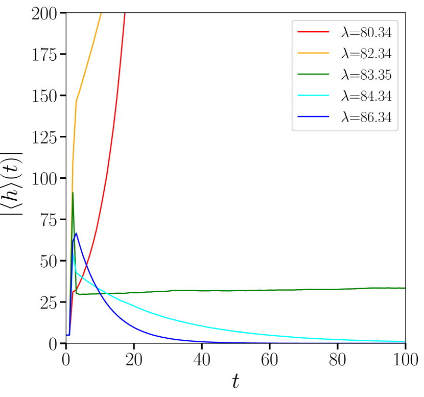
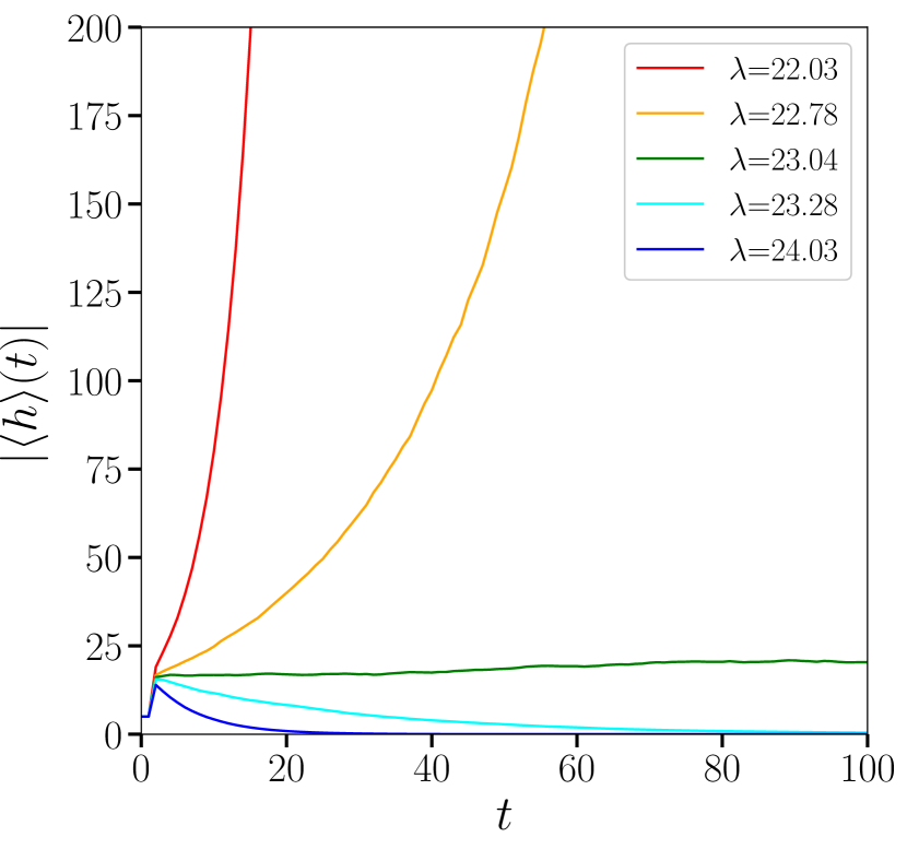
Figure 1: Evolution of the first moment of the $h$ population, $\langle h\rangle(t)$, according to the population dynamics algorithm as outlined in section 4, with population size of $N_{P}=10^{5}$ and where $t$ is measured in sweeps. The control parameters in this figure are chosen as $q=8$, $\alpha=\sqrt{5/4}$ and $p(K)=\delta_{K,1}$ for the left figure and $p(K)=\Theta(1-K)\Theta(K)$ for the right figure. The different curves correspond to ascending values of $\lambda$ (top to bottom), the parameter that governs the convergence of the algorithm. For $\lambda<\Big{\langle}\lambda_{1}\Big{\rangle}$ (red and orange lines) the population diverges, for $\lambda>\Big{\langle}\lambda_{1}\Big{\rangle}$ (blue and cyan lines) it vanishes, and only when $\lambda=\Big{\langle}\lambda_{1}\Big{\rangle}$ (green line), stability is reached. The rate of divergence/decay depends on the amount by which $\lambda$ deviates from $\Big{\langle}\lambda_{1}\Big{\rangle}$.

Specifying to the case where $\lambda=\langle\lambda_{1}\rangle$ and nontrivial stability is achievable, it is possible to identify multiple fixed points for the densities $\pi$ and $\hat{\pi}$ that satisfy the first two equations in (69) by adjusting the initial populations. However, incorporating the third equation in (69) uniquely determines the solution. Once the algorithm identifies the value of $\lambda$ that allows nontrivial stable populations, the third condition in (69) can be fulfilled by rescaling the $h$ and $\hat{h}$ populations, yielding a solution that satisfies (69) in its entirety. This rescaling is always allowed due to the linear nature of the recursion governing their updates [53].

Given the behaviour described above, the strategy for pinning down the value of $\lambda$ under which stability can be reached, is to start with a large value, determined by a proper upper bound for $\Big{\langle}\lambda_{1}\Big{\rangle}$. Then, while running the algorithm, one monitors the dynamics of the populations’ first moment, and gradually decreases the value of $\lambda$ until they stabilise. A plausible upper bound that can be used as a starting point is $\lambda^{*}=\left[\max\left(|\zeta^{-}|,|\zeta^{+}|\right)\right]^{2}DT$, where $\zeta^{-}$ ($\zeta^{+}$) is the lower (upper) bound of the support of $p(K)$, while $D$ and $T$ are the largest integers that satisfy $Mp_{\alpha q}(D)\geq 1$ and $Np_{\alpha^{-1}q}(T)\geq 1$ respectively, with $p_{m}$ being the Poisson distribution with mean $m$ (See B for a proof).

In Fig. 2 we present the scaling of $\Big{\langle}\lambda_{1}\Big{\rangle}$ with the dimensions of the matrix $\bm{X}$, under the following choice of control parameters: (a) $\alpha=\sqrt{5/4}$, $q=11.8$ and $p(K)=\delta_{K,1}$; (b) $\alpha=\sqrt{5/4}$, $q=8$ and $p(K)=\Theta(K)\Theta(1-K)$, with $\Theta(\cdot)$ being the Heaviside function [i.e., $K\in(0,1)$ with uniform probability]. As outlined in section 3, we computed the leading behavior of $\Big{\langle}\lambda_{1}\Big{\rangle}$ as both of $\bm{J}$’s linear dimensions tend to infinity. Therefore, our analysis does not account for any finite size effects. However, in Fig. 2 we show that these correction are negligible compared to the leading behavior, which is perfectly captured by our analysis. Specifically, even for a relatively small matrix of size $100\times 80$, finite size corrections are responsible for a deviation of merely $\sim 4\%$. When the matrix size is further increased, the numerical results quickly align with our analytical results, to the extent that the two are indistinguishable within our measurement’s resolution.

In figure 3 we compare results for $\Big{\langle}\lambda_{1}\Big{\rangle}$ obtained from the replica analysis (solid line) and direct numerical diagonalisation (circles), as a function of $q$, which regulates the average density of nonzero elements in $\bm{X}$. In this figure we chose $\alpha=\sqrt{5/4}$ and the weight distributions (a) $p(K)=\delta_{K,1}$; (b) $p(K)=\Theta(1-K)\Theta(K)$. In light of Fig. 2, the numerical data was obtained by averaging over $10^{2}$ realizations of $\bm{X}$ with a fixed size of $5,000\times 4,000$, such that finite size corrections are negligible. Within this framework, we find excellent agreement between the numerical and analytical results.

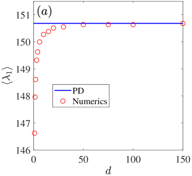
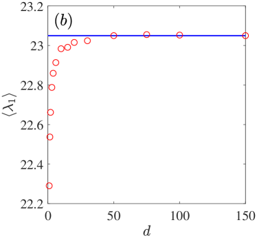
Figure 2: Scaling of $\Big{\langle}\lambda_{1}\Big{\rangle}$ with the dimensions of the matrix $\bm{X}$. This figure shows $\Big{\langle}\lambda_{1}\Big{\rangle}$, collected from direct numerical diagonalisation of $10^{2}$ realisations of $\bm{J}$ (circles), as the size of the matrix $\bm{X}$ is increased, while the ratio $\alpha=\sqrt{N/M}$ is kept fixed. The scaling parameter $d$ is defined such that each data point was obtained using a matrix $\bm{X}$ of size $(100\cdot d)\times(80\cdot d)$. The dashed line represents the results obtained from the replica analysis, using the population dynamics algorithm, using populations of size $N_{P}=10^{5}$. The set of control parameters used here is (a) $\alpha=\sqrt{5/4}$, $q=11.8$ and $p(K)=\delta_{K,1}$; (b) $\alpha=\sqrt{5/4}$, $q=8$ and $p(K)=\Theta(K)\Theta(1-K)$. As can be observed from the figure, even for a relatively small matrix of size $100\times 80$, finite size effects are responsible for a deviation of only up to $\sim 4\%$ from the analytical result. For a matrix $\sim 50$ times bigger than that, this deviation drops below the measurement’s resolution.

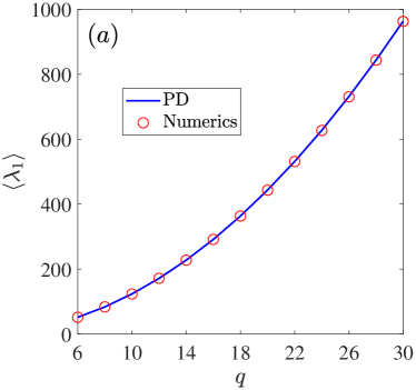
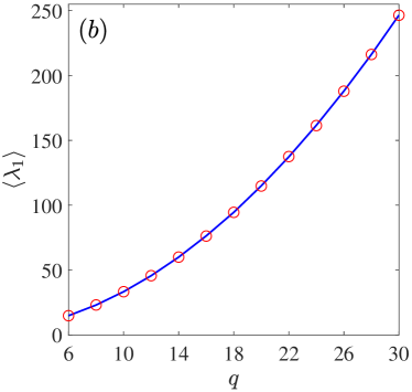
Figure 3: We show $\Big{\langle}\lambda_{1}\Big{\rangle}$ as obtained by both population dynamics (solid line) and direct numerical diagonalisation (circles) as a function of $q$, which regulates the average density of nonzero elements in $\bm{X}$. For this analysis, we used $\alpha=\sqrt{5/4}$ and set the weight distribution to (a) $p(K)=\delta_{K,1}$, and (b) $p(K)=\Theta(1-K)\Theta(K)$. In view of Fig. 2, the numerical data represents an average over $10^{2}$ realizations of $\bm{X}$, each of fixed and large dimensions $5,000\times 4,000$. Under these conditions, the numerical and analytical results are in very strong agreement.

5 Conclusions

In summary, we have developed a replica formalism to compute the average largest eigenvalue of sparse correlation matrices of the form $\bm{X}^{T}\bm{X}$ whose non-zero entries are drawn from a non-zero mean weight distribution $p(K)$, which leads to an isolated largest eigenvalue. The problem can be recast as the optimisation of a quadratic Hamiltonian on the sphere. By introducing the zero-temperature limit $\beta\rightarrow\infty$, the Gibbs measure concentrates around the ground state, represented by the top eigenvector of the Hamiltonian. To tackle this optimization problem, we employed the replica method. This involves evaluating the average of powers of the partition function $Z$, followed by taking the thermodynamic limit $M\rightarrow\infty$, as well as the replica ($n\to 0$) and zero-temperature ($\beta\to\infty$) limits.

This formulation leads to a system of self-consistent equations governed by the parameter $\lambda$, explicitly given by equations (69). We solved this system using a population dynamics algorithm. Within this framework, we identified $\Big{\langle}\lambda_{1}\Big{\rangle}$, the average largest eigenvalue of our sparse matrix $\bm{X}^{T}\bm{X}$, as the critical value of the control parameter $\lambda$ for which the populations converge: if $\lambda<\Big{\langle}\lambda_{1}\Big{\rangle}$, the variables diverge in norm, while if $\lambda>\Big{\langle}\lambda_{1}\Big{\rangle}$, they converge to zero. Numerical simulations of the population dynamics yielded excellent agreement between the convergence parameter and the results obtained from direct numerical diagonalisation of the matrix. This agreement holds for both degenerate weight distribution, $p(K)=\delta_{K,1}$, and for uniform weight distribution within the range $K\in[0,1]$, i.e., $p(K)=\Theta(K)\Theta(1-K)$. Extending our analysis to capture the non-gapped case and establishing connections between the properties of $p(K)$ and various aspects of the detachment transition are the topics of forthcoming publications.

Our work further advanced the literature by demonstrating analytically the equivalence of $\lambda$ and $\Big{\langle}\lambda_{1}\Big{\rangle}$, thereby providing a robust validated method of solving the average largest eigenvalue problem for sparse matrices of the form $\bm{X}^{T}\bm{X}$ across diverse different weight distributions $p\left(K\right)$.

Appendix A Performing the Average in (13)

In this appendix, we show how to compute the average

$$\Big{\langle}\prod_{i=1}^{M}\prod_{j=1}^{N}\exp\left(\beta X_{ji}\sum_{a=1}^{n}v_{ia}u_{ja}\right)\Big{\rangle}\ ,$$ (74)

in the $q\ll\sqrt{NM}$ limit. This average is performed over different realizations of the $N\times M$ random matrix $\bm{X}$, whose entries are i.i.d RVs, expressed as $X_{ji}=c_{ji}K_{ji}$, and are drawn from

$$P\left(X_{ji}\right)=\left[\frac{q}{\sqrt{NM}}\delta_{c_{ji},1}+\left(1-\frac{q}{\sqrt{NM}}\right)\delta_{c_{ji},0}\right]p\left(K_{ji}\right)\ ,$$ (75)

with $p(K)$ being weight distribution. First, we use the independence of the entries to factorize the average,

$$\Big{\langle}\prod_{i=1}^{M}\prod_{j=1}^{N}\exp\left(\beta X_{ji}\sum_{a=1}^{n}v_{ia}u_{ja}\right)\Big{\rangle}=\prod_{i=1}^{M}\prod_{j=1}^{N}\Big{\langle}\exp\left(\beta cK\sum_{a=1}^{n}v_{ia}u_{ja}\right)\Big{\rangle}_{c,K},$$ (76)

where $\Big{\langle}\cdot\Big{\rangle}_{c,K}$ denotes averaging over a single instance of the RVs $c$ and $K$. Next, we average over the $c$’s and take the $q\ll\sqrt{NM}$ limit to obtain

$$\Big{\langle}\prod_{i=1}^{M}\prod_{j=1}^{N}\exp\left(\beta X_{ji}\sum_{a=1}^{n}v_{ia}u_{ja}\right)\Big{\rangle} =\prod_{i=1}^{M}\prod_{j=1}^{N}\left[1+\frac{q}{\sqrt{NM}}\left(\Big{\langle}\mathrm{e}^{\beta K\sum_{a=1}^{n}v_{ia}u_{ja}}\Big{\rangle}_{K}-1\right)\right]$$

$$\simeq\exp\left[\frac{q}{\sqrt{NM}}\sum_{i=1}^{M}\sum_{j=1}^{N}\left(\Big{\langle}\mathrm{e}^{\beta K\sum_{a=1}^{n}v_{ia}u_{ja}}\Big{\rangle}_{K}-1\right)\right],$$ (77)

which matches the result in (13).

Appendix B Upper Bound for $\Big{\langle}\lambda_{1}\Big{\rangle}$

In this appendix we show that typically, $\lambda_{1}$ satisfies

$$\lambda_{1}\leq\left[\max\left(|\zeta^{-}|,|\zeta^{+}|\right)\right]^{2}DT\ ,$$ (78)

where $\zeta^{-}$ ($\zeta^{+}$) is the lower (upper) bound of the support of $p(K)$, while $D$ and $T$ are the largest integers that satisfy $Mp_{\alpha q}(D)\geq 1$ and $Np_{\alpha^{-1}q}(T)\geq 1$ respectively ($p_{m}$ being the Poisson distribution with mean $m$). Our starting point is the identification of $\lambda_{1}$ with the square of the spectral norm of the matrix $\bm{X}$. According to identity 15.511.1 from [76], the spectral norm obeys

$$\lambda_{1}\leq\left(\max_{1\leq j\leq M}\sum_{i=1}^{N}|X_{ij}|\right)\left(\max_{1\leq i\leq N}\sum_{j=1}^{M}|X_{ij}|\right)\ .$$ (79)

Since $X_{ij}=c_{ij}K_{ij}$ [Eq. (1)], we can use the fact that $p(K)$ has a bounded support to write

$$\lambda_{1}\leq\left[\max\left(|\zeta^{-}|,|\zeta^{+}|\right)\right]^{2}\left(\max_{1\leq j\leq M}\sum_{i=1}^{N}c_{ij}\right)\left(\max_{1\leq i\leq N}\sum_{j=1}^{M}c_{ij}\right).$$ (80)

Furthermore, since the $c_{ij}$’s are Bernoulli RVs with ‘success’ probability $q/\sqrt{NM}=\alpha q/N=\alpha^{-1}q/M$, in the $N,M\rightarrow\infty$ limit, each column and each row is associated with a Poissonian RV,

$$\sum_{i=1}^{N}c_{ij}\sim p_{\alpha q}\ ,$$ (81)

$$\sum_{j=1}^{M}c_{ij}\sim p_{\alpha^{-1}q}\ ,$$ (82)

respectively. Considering samples of $M$ columns and $N$ rows, typically, the maximal values of RVs drawn from these samples ($D$ and $T$) would be the largest integers satisfying

$$Mp_{\alpha q}(D)\geq 1\ ,$$ (83)

$$Np_{\alpha^{-1}q}(T)\geq 1\ ,$$ (84)

respectively. Hence, setting aside extreme cases that are statistically rare, we have

$$\sum_{i=1}^{N}c_{ij}\leq D$$ (85)

$$\sum_{j=1}^{M}c_{ij}\leq T\ .$$ (86)

Inserting (86) into (80) we obtain our desired result, Eq. (78).

References

- [1] J. Fan, F. Han, and H. Liu, National Science Review 1, 293 (2014)
- [2] I. Jolliffe, Principal Component Analysis, Springer Series in Statistics (Springer, 2002)
- [3] G. James, D. Witten, T. Hastie, and R. Tibshirani, An Introduction to Statistical Learning: with Applications in R, Springer Texts in Statistics (Springer New York, 2014)
- [4] K. Sachs, O. Perez, D. Pe’er, D. A. Lauffenburger, and G. P. Nolan, Science 308, 523 (2005)
- [5] A. J. Butte, P. Tamayo, D. Slonim, T. R. Golub, and I. S. Kohane, Proceedings of the National Academy of Sciences 97, 12182 (2000)
- [6] D. M. Witten, R. Tibshiran, and T. Hastie, Biostatistics 10, 515 (2009)
- [7] Y. Deng, Y.-H. Jiang, Y. Yang, Z. He, F. Luo, and J. Zhou, BMC Bioinformatics 13, 113 (2012)
- [8] Z. D. Kurtz, C. L. Müller, E. R. Miraldi, D. R. Littman, M. J. Blaser, and R. A. Bonneau, PLOS Computational Biology 11, 1 (2015)
- [9] O. Levy and Y. Goldberg, Neural Information Processing Systems 27, 2177 (2014)
- [10] J. P. Bouchaud, arXiv:0903.2428 (2009)
- [11] M. E. J. Newman, SIAM Rev. 45, 167 (2003)
- [12] J. Fan, Y. Liao, and H. Liu, The Econometrics Journal 19, C1 (2016)
- [13] J. Wishart, Biometrika 20A, 32 (1928)
- [14] A. Gupta and D. Nagar, Matrix Variate Distributions, Monographs and Surveys in Pure and Applied Mathematics (Taylor & Francis, 1999)
- [15] F. J. Dyson, Journal of Mathematical Physics 3, 140 (1962)
- [16] F. J. Dyson, Journal of Mathematical Physics 3, 157 (1962)
- [17] F. J. Dyson, Journal of Mathematical Physics 3, 166 (1962)
- [18] P. Vivo, S. N. Majumdar, and O. Bohigas, J. Phys. A: Math. Theor. 40, 4317 (2007)
- [19] E. Katzav and I. Pérez Castillo, Phys. Rev. E 82, 040104 (2010)
- [20] S. N. Majumdar and P. Vivo, Phys. Rev. Lett. 108, 200601 (2012)
- [21] S. N. Majumdar and M. Vergassola, Phys. Rev. Lett. 102, 060601 (2009)
- [22] J. A. Zavatone-Veth and C. Pehlevan, SciPost Phys. Core 6, 026 (2023)
- [23] T. Rogers, I. Pérez Castillo, R. Kühn, and K. Takeda, Phys. Rev. E 78, 031116 (2008)
- [24] T. Nagao and T. Tanaka, J. Phys. A: Math. Theor. 40, 4973 (2007)
- [25] I. P. Castillo and F. L. Metz, Phys. Rev. E 97, 032124 (2018)
- [26] G. Livan, M. Novaes, and P. Vivo, Introduction to Random Matrices: Theory and Practice (Springer, 2018)
- [27] P. J. Forrester, Constr. Approx. 41, 589–613 (2015)
- [28] R. Kühn, J. Phys. A: Math. Theor. 41, 295002 (2008)
- [29] T. Rogers and I. Pérez Castillo, Phys. Rev. E 79, 012101 (2009)
- [30] T. Rogers, C. P. Vicente, K. Takeda, and I. Pérez Castillo, J. Phys. A: Math. Theor. 43, 195002 (2010)
- [31] F. L. Metz, I. Neri, and D. Bollé, Phys. Rev. E 82, 031135 (2010)
- [32] F. L. Metz, I. Neri, and D. Bollé, Phys. Rev. E 84, 055101 (2011)
- [33] I. Neri and F. L. Metz, Phys. Rev. Lett. 109, 030602 (2012)
- [34] D. Bollé, F. L. Metz, and I. Neri, Spectral analysis, differential equations and mathematical physics: A festschrift in honor of fritz gesztesy’s 60th birthday, (Amer. Math. Soc., 2013) Chap. On the spectra of large sparse graphs with cycles, pp. 35–58
- [35] F. L. Metz, G. Parisi, and L. Leuzzi, Phys. Rev. E 90, 052109 (2014)
- [36] I. Neri and F. L. Metz, Phys. Rev. Lett. 117, 224101 (2016)
- [37] I. M. Johnstone, The Annals of Statistics 2, 295 (2001)
- [38] K. V. Mardia, J. T. Kent, and J. M. Bibby, Multivariate Analysis (Academic Press, 1979)
- [39] R. Monasson and D. Villamaina, Europhysics Letters, 112, 50001 (2015)
- [40] Z. Bai and J. W. Silverstein, Spectral Analysis of Large Dimensional Random Matrices (Springer New York, 2010)
- [41] P. Stoica and M. Cedervall, IFAC Proceedings Volumes 29, 4098 (1996)
- [42] P. Bianchi, M. Debbah, M. Maida and J. Najim, IEEE Transactions on Information Theory 57, 2400 (2011)
- [43] R. R. Nadakuditi and A. Edelman, IEEE Transactions on Signal Processing 56, 2625 (2008)
- [44] S. Peche, Probab. Theory Relat. Fields 143, 481 (2009)
- [45] N. E. Karoui, Annals of Probability 35, 663 (2005)
- [46] Z. Bao, G. Pan, and W. Zhou, Annals of Statistics 43, 382 (2015)
- [47] S. P. Natesh and J. Yin, Ann. Appl. Probab. 24, 935 (2014)
- [48] X. Ding, F. Yang, Ann. Appl. Probab. 28, 1679 (2018)
- [49] J. Y. Hwang, J. O. Lee, and W. Yang, Bernoulli 26, 2400 (2019)
- [50] A. Auffinger and S. Tang, Stochastic Processes and their Applications 126, 3310 (2015)
- [51] J. Baik, G. B. Arous, and S. Péché, Ann. Probab. 33, 1643 (2005)
- [52] K. Bassler, P. Forrester, and N. Frankel, J. Math. Phys. 50, 1089 (2008)
- [53] V. A. Susca, P. Vivo, and R. Kühn, J. Phys. A: Math. Theor. 52, 485002 (2019)
- [54] V. A. Susca, P. Vivo, and R. Kühn, J. Phys. A: Math. Theor. 54, 015004 (2020)
- [55] V. A. Susca, P. Vivo, and R. Kühn, SciPost Phys. Lect. Notes, 33 (2021)
- [56] F. Zamponi, ArXiv: abs/1008.4844 (2010)
- [57] M. Mezard, G. Parisi, and M. Virasoro, Spin Glass Theory and Beyond, Lecture Notes in Physics Series (World Scientific, 1987)
- [58] S. F. Edwards and R. C. Jones, J. Phys. A: Math. Gen. 9, 1595 (1976)
- [59] G. J. Rodgers and C. D. Dominicis, J. Phys. A: Math. Gen. 23, 1567 (1990)
- [60] P. Akara-pipattana and O. Evnin, ArXiv: 2410.00355 (2024)
- [61] G. Biroli and R. Monasson, J. Phys. A: Math. Gen. 32, L255 (1999)
- [62] G. Semerjian and L. F. Cugliandolo, J. Phys. A: Math. Gen. 35, 4837 (2002)
- [63] G. Bianconi, ArXiv: 0804.1744 (2008)
- [64] R. Kühn, J. v. Mourik, M. Weigt, and A. Zippelius, J. Phys. A: Math. Theor. 40, 9227 (2007)
- [65] D. S. Dean, J. Phys. A: Math. Gen. 35, L153 (2002)
- [66] F. L. Metz and D. A. Stariolo, Phys. Rev. E 92, 042153 (2015)
- [67] F. L. Metz and I. Pérez Castillo, Phys. Rev. Lett. 117, 104101 (2016)
- [68] F. L. Metz and I. Pérez Castillo, Phys. Rev. B 96, 064202 (2017)
- [69] F. A. López and A. C. C. Coolen, J. Phys. A: Math. Theor. 53, 065002 (2020)
- [70] B. Bollobas, Random Graphs, 2nd ed. (Cambridge University Press, 2001)
- [71] M. Mezard and G. Parisi, Eur. Phys. J. B 20, 217 (2001)
- [72] L. Zdeborová and F. Krzakala, Advances in Physics 65, 453 (2015)
- [73] R. Kühn and T. Rogers, Europhysics Letters 118, 68003 (2017)
- [74] R. Kühn, Phys. Rev. E 110, L032301 (2024)
- [75] S. Bartolucci, F. Caccioli, F. Caravelli, and P. Vivo, Proceedings of the National Academy of Sciences of the United States of America 121, 40 (2024).
- [76] I. S. Gradshteyn and I. M. Ryzhik, Table of Integrals, Series, and Products, 7th Edition (Academic Press, 2007)