Minimax discrete distribution estimation with self-consumption

Millen Kanabar and Michael Gastpar
School of Computer and Communication Sciences, EPFL
Abstract

Learning distributions from i.i.d. samples is a well-understood problem. However, advances in generative machine learning prompt an interesting new, non-i.i.d. setting: after receiving a certain number of samples, an estimated distribution is fixed, and samples from this estimate are drawn and introduced into the sample corpus, undifferentiated from real samples. Subsequent generations of estimators now face contaminated environments, an effect referred to in the machine learning literature as self-consumption. In this paper, we study the effect of such contamination from previous estimates on the minimax loss of multi-stage discrete distribution estimation.

In the data accumulation setting, where all batches of samples are available for estimation, we provide minimax bounds for the expected $\ell_{2}^{2}$ and $\ell_{1}$ losses at every stage. We show examples where our bounds match under mild conditions, and there is a strict gap with the corresponding oracle-assisted minimax loss where real and synthetic samples are differentiated. We also provide a lower bound on the minimax loss in the data replacement setting, where only the latest batch of samples is available, and use it to find a lower bound for the worst-case loss for bounded estimate trajectories.

I Introduction

The problem of estimating distributions from their samples arises naturally in various contexts, and has been studied in depth in the literature. The exact minimax loss of discrete distribution estimation under the $\ell_{2}^{2}$ metric, among others, was found in [1], and was studied under $\ell_{1}$ metric e.g. in [2, 3, 1]. Evidently, the results of these estimations are often themselves valid distributions. These estimates can then themselves be used to generate new samples in the same alphabet.

In cases where distribution estimation is performed in batches, samples generated from estimates at some stage can be reintroduced into subsequent batches of ‘real’ samples, thereby affecting future performance. This phenomenon has been widely observed, for example, in the context of generative machine learning, where distributions are estimated primarily to produce new samples, in part because it is significantly cheaper to generate synthetic samples. This has also led to fears that synthetic samples might significantly contaminate real databases such as the Internet [4]. It has been observed empirically e.g. in [5, 6] that this process, without external mitigation, leads to ‘model collapse’: worsening performance with every iteration where samples from previous stages are introduced into the training pool.

The self-referential nature of the sampling process causes the distributions of later samples to depend non-trivially on the previous batches, and thus prevents the direct use of already existing results from the distribution estimation literature. In this paper, we study the properties of such sequences of estimates under a minimax lens.

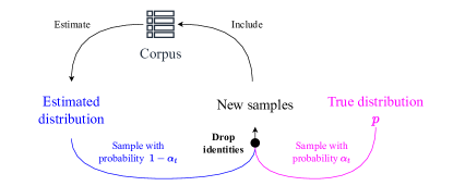
A sketch of the data production workflow considered in our paper is shown in Figure 1. A crucial aspect of the model is that the corpus does not include the identities of the source of the samples, i.e. whether they are real or synthetic. In the data accumulation setting, new samples are continually added to the corpus at every stage, whereas it consists of only fresh samples in the data replacement setting. This mirrors quite a few variants considered in the generative machine learning literature. In this paper, we assume that each sample is drawn from either the true underlying distribution or the previous estimate based on the outcome of a coin flip with time-dependent bias $\alpha_{t}$, assumed to be known to the estimator.

Refer to caption
Figure 1: The estimation workflow under self-consumption

I-A Related work

Model collapse in settings containing feedback loops with different mechanisms of mixing synthetic data with old and new real samples was first studied empirically in [5] and [6]. Specifically, the case for discrete distribution estimation in a fully synthetic loop, wherein, at every stage, the estimator only has access to samples generated from the distribution estimated at the previous stage was considered as a motivating example in the analysis of [5].

An upper bound on the proportion of synthetic data for in-loop stability of parametric generative models trained on freshly generated (mixed) samples at each stage was provided in [7]. The evolution of parametric models and nonparametric kernel density estimators trained on fully synthetic and mixed data loops was described in [8]. Model collapse in regression models and mitigation strategies are discussed in [9, 10].

I-B Contributions

In this work, we pose the multi-stage distribution estimation problem with self-consumption of samples, which has not been studied in the minimax setting before in the literature. Moreover, we provide the first (to the best of our knowledge) minimax lower bounds on the $\ell_{2}^{2}$ and $\ell_{1}$ losses at each stage in terms of properties of the estimates at previous stages in Theorem 1 (for the data accumulation workflow) and Corollary 3 (for the data replacement workflow).

We also propose a sequence of estimators that is order optimal under certain regimes with stage-wise performance guarantees in Theorem 2, and show examples of problem parameters where the conditions for order optimality are met in the data accumulation workflow. We also show that the ratio of minimax loss to the minimax loss in the presence of identity information grows infinitely large in such cases.

For example, when the number of samples added in stage $t$ increases linearly with $t,$ but each stage only contains, on average, $\sqrt{t}$ samples from the true distribution, then we show that the loss under self-consumption behaves as $1/\sqrt{t}$ while the oracle bound, with known sample identities, would behave as $1/t.$

Finally, we use our lower bound for the data replacement workflow to find a lower bound on the worst-case loss given a time-independent upper bound.

I-C Notation

Deterministic quantities and functions are represented by lowercase Greek and Roman alphabets; random variables are represented by uppercase Roman alphabets. The probability simplex corresponding to the alphabet of size $k$ is denoted as $\Delta_{k}$. The $j^{\mathrm{th}}$ component of a discrete distribution $P$ or vector $p$ is indexed by square brackets as $P[j]$ and $p[j]$ respectively, and the probability of an event $A$ under distribution $Q$ is denoted as $Q\{A\}$. The first subscript of quantities in sequences denotes the index in the sequence, subsequent ones are used to denote other parameters when needed. The $n$-fold product of a distribution $Q$ is denoted as $Q^{n}$. For $t\geq 0$ and functions $f,g$, we write $g(t)=\Theta(f(t))$ if there exist constants $a_{1},a_{2}$ such that $a_{1}f(t)\leq g(t)\leq a_{2}f(t)\ \forall t\geq 0$. We use $[a:b]$ to denote $\{x\in\mathbb{N}:a\leq x\leq b\}$. The unit vector in with component $j$ equal to $1$ is denoted as $e_{j}$.

II Problem Setup

Definition 1 (Self-consuming estimation)

For a distribution $p\in\Delta_{k}$, a self-consuming sequence of sample-estimator pairs with sample sizes $(n_{t})_{t\geq 0}$ and sampling probabilities $(\alpha_{t})_{t\geq 1}$ is a sequence $\left(X_{t}^{n_{t}},\hat{p}_{t}(\cdot)\right)_{t\geq 0}$ such that

  • $X_{0}^{n_{0}}\sim p^{n_{0}}$, and

  • $X_{t+1}^{n_{t+1}}\sim\left(\tilde{P}({p,\hat{P}_{t},\alpha_{t+1}})\right)^{n_{t+1}}$,
    where $\tilde{P}({p_{1},p_{2},\alpha}):=\alpha p_{1}+(1-\alpha)p_{2}$, and $\hat{P}_{t}:=\hat{p}_{t}\left(X_{0}^{n_{0}},\dots,X_{t}^{n_{t}}\right)$ for every $t\geq 0$.

The joint distribution of the random vector $(X_{0}^{n_{0}},\dots,X_{t}^{n_{t}})$ is denoted as $\bar{\mathbf{P}}_{t,({p,\{n_{i},\alpha_{i}:i\geq 0\}})}$. We drop the sample sizes and sampling probabilities when they are obvious from the context. By convention, $\alpha_{0}=1$.

The definition of this sequence encapsulates the following process: at stage 0, an estimate $\hat{P}_{0}$ is produced using a batch of $n_{0}$ i.i.d. samples from $p$. At every subsequent stage $t$, a batch of $n_{t}$ samples is produced, with each sample being distributed as $p$ with probability $\alpha_{t}$ and as $\hat{P}_{t-1}$ with probability $1-\alpha_{t}$.

For a sequence of estimators $\hat{p}_{t}(\cdot)$, we consider the minimax loss under the $\ell_{2}^{2}$ and $\ell_{1}$ loss metrics.

Definition 2 (Minimax loss)

For a given loss metric $\ell$, sequences $\{n_{i},\alpha_{i}:i\geq 0\}$ and fixed estimators $\hat{p}_{i}(\cdot),i\in[1:t]$, the minimax loss at stage $t$ is defined as

$\displaystyle r^{\ell}_{t,k}=\inf_{\hat{p}_{t}}\sup_{p\in\Delta_{k}}E[\ell(\hat{p}_{t}(X_{0}^{n_{0}},\dots,X_{t}^{n_{t}}),p)]$

where the expectation is with respect to the joint distribution $\bar{\mathbf{P}}_{t,(p,\{n_{i},\alpha_{i}:i\geq 0\})}$.

It is important to note that the minimax loss is defined for the estimator at every stage $t$ while fixing the estimators in all the previous stages. This follows from the process of designing the estimators: they are selected sequentially at every stage, without concern for how the samples generated from these estimates might influence future samples.

III Main Results

The main contributions of this paper are upper and lower bounds on the minimax loss of the self-consuming sequence at an arbitrary stage $t\geq 0$. The bounds are stated as follows:

Theorem 1 (Minimax lower bound)

Fix $\hat{p}^{(i)},i{\in}[0{:}t{-}1]$. Let $g_{0}(\epsilon)=0\ \forall\epsilon$. For $i\neq 0$, let

$\displaystyle g_{i}(\epsilon):=\sup_{p}\max_{j}\bar{\mathbf{P}}_{i-1,({p})}\left\{\hat{P}_{i-1}[j]<p[j]-\epsilon\right\}$

be the worst case probability of an $\epsilon$-error under $\bar{\mathbf{P}}_{i,({p})}$. Denote $h_{t}(\nicefrac{{1}}{{4k}}):=\sum_{i=0}^{t}n_{i}\alpha_{i}g_{i}(\nicefrac{{1}}{{4k}})$.

The minimax loss for the self-consuming estimator-sample sequence at stage $t$ under $\ell_{2}^{2}$ and $\ell_{1}$ losses is lower bounded, respectively, as

$\displaystyle r^{\ell_{2}^{2}}_{t,k}\geq$ $\displaystyle\frac{\nicefrac{{1}}{{512}}}{\sum_{i=0}^{t}n_{i}\alpha_{i}^{2}+h_{t}({\nicefrac{{1}}{{4k}}})}$ (1)
$\displaystyle r^{\ell_{1}}_{t,k}\geq$ $\displaystyle\sqrt{\frac{\nicefrac{{k}}{{4096}}}{\sum_{i=0}^{t}n_{i}\alpha_{i}^{2}+h_{t}({\nicefrac{{1}}{{4k}}})}}$ (2)

whenever $\sum_{i=0}^{t}n_{i}\alpha_{i}^{2}+h_{1/4k}(t)\geq k/4$.

Theorem 2 (Upper bound)

Let $n_{i}\alpha_{i}\leq\sum_{j=0}^{i}n_{j}\alpha_{j}^{2}$ for every $i\leq t$. Then there exists an estimator-sample sequence for which the $\ell_{2}^{2}$ and $\ell_{1}$ losses are upper bounded as

$\displaystyle\sup_{p}E[\ell_{2}^{2}(p,\hat{p}_{t}(X_{0}^{n_{0}},\dots,X_{t}^{n_{t}}))]\leq$ $\displaystyle\frac{1-\nicefrac{{1}}{{k}}}{\sum_{i=0}^{t}n_{i}\alpha_{i}^{2}}$ (3)
$\displaystyle\sup_{p}E[\ell_{1}(p,\hat{p}_{t}(X_{0}^{n_{0}},\dots,X_{t}^{n_{t}}))]\leq$ $\displaystyle\sqrt{\frac{k-1}{\sum_{i=0}^{t}n_{i}\alpha_{i}^{2}}}$ (4)

Theorem 1 can also be modified for the data replacement setting to obtain the following corollary:

Corollary 3 (Minimax lower bound with data replacement)

Let $\mathbf{Q_{p}}$ be a distribution on $\Delta_{k}$ that depends on $p$, and let $\hat{P}\sim\mathbf{Q_{p}}$ be an estimate of $p$. Let samples $X_{1}^{n_{1}}\sim\tilde{P}({p,\hat{P},\alpha})^{n_{1}}$. Denote $h({\epsilon}):=n_{1}\alpha\sup_{p}\max_{j}\mathbf{Q_{p}}\{\hat{P}[j]<p[j]-\epsilon\}$. The minimax $\ell_{2}^{2}$ and $\ell_{1}$ losses of an estimator $\hat{p}_{1}(X_{1}^{n_{1}})$ are lower bounded as

$\displaystyle r^{\ell_{2}^{2}}_{k,\{\alpha,n_{1}\}}\geq$ $\displaystyle\frac{\nicefrac{{1}}{{512}}}{n_{1}\alpha^{2}+h({\nicefrac{{1}}{{4k}}})}$ (5)
$\displaystyle r^{\ell_{1}}_{k,\{\alpha,n_{1}\}}\geq$ $\displaystyle\sqrt{\frac{\nicefrac{{k}}{{4096}}}{n_{1}\alpha^{2}+h({\nicefrac{{1}}{{4k}}})}}$ (6)

whenever $n_{1}\alpha^{2}+h\left({\nicefrac{{1}}{{4k}}}\right)\geq k/4$.

IV Discussion

IV-A The error term $h_{t}({\nicefrac{{1}}{{4k}}})$

The multi-stage lower bounds depend on the performance of estimators in previous stages through the probabilities $g_{i-1}\left(\nicefrac{{1}}{{4k}}\right)$. It is perhaps surprising that the lower bounds decrease as these probabilities increase. The source of this apparent improvement is the looser upper bound on the KL divergence in (11) when the previous estimators perform badly. This suggests that it might be easier for an estimator to perform well when the synthetic samples are from a distribution sufficiently removed from the real one.

The estimator analyzed in the upper bound section does not share this behavior, leading to a gap between the upper and lower bounds in the case where the proportion of real samples decays very rapidly. The estimator is also kept unbiased at every stage via assumptions on the problem parameters; this helps keep the analysis from becoming almost prohibitively cumbersome. A careful analysis of a more general class of linear estimators might help bridge the gap with the lower bounds or drop the assumptions required. Alternatively, a tighter analysis bounding the aforementioned divergence might lead to a lower bound that matches the upper bound wherever valid.

IV-B Comparison against oracle-assisted minimax loss

To understand the impact of not knowing the source identity on the minimax loss, it is useful to compare the upper and lower bounds presented above to the ones when the identity of the source of each sample is known in the form of an auxiliary random vector $W:=W_{i}^{n_{i}}\sim(\mathrm{Bern}(\alpha_{i}))^{n_{i}},i\in\{1,\dots,t\}$ provided to the estimator by an oracle.

Lemma 4 (Oracle-assisted minimax loss)

There exist positive constants $c_{1},c_{2}$ such that the minimax loss $r^{\ell_{2}^{2},\mathrm{oracle}}_{t,k}$ of self-consuming estimation with information on source identity is bounded between

$\displaystyle\frac{c_{1}}{\sum_{i=0}^{t}n_{i}\alpha_{i}}\leq r^{\ell_{2}^{2},\mathrm{oracle}}_{t,k}\leq\frac{c_{2}}{\sum_{i=0}^{t}n_{i}\alpha_{i}}.$
Proof:

Using Lemma 5 and the chain rule of the KL divergence, along with the fact that

$\displaystyle D(\tilde{P}({p_{v},\hat{P}^{(i)},\alpha})\|\tilde{P}({p_{v-2e_{j}},\hat{P}^{(i)},\alpha})|W)=\alpha D(p_{v}\|p_{v-2e_{j}})$

leads to an $\ell_{2}^{2}$ lower bound of $\frac{1}{512\sum_{i=0}^{t}n_{i}\alpha_{i}}$. The empirical distribution of the real samples can be shown to have an $\ell_{2}^{2}$ loss within a constant factor of $\frac{1-\nicefrac{{1}}{{k}}}{\sum_{i=0}^{t}n_{i}\alpha_{i}}$ via a Chernoff-style argument. Similar bounds can be obtained for the $\ell_{1}$ loss. ∎

The absence of source information at the estimator leads to a penalty factor of roughly $\max(\alpha_{i},g_{i-1}(\nicefrac{{1}}{{4k}}))$ in the ‘effective sample size’ of each batch. This can lead to large significant gaps between the base and oracle-assisted losses. Depending on whether or not the $\alpha_{i}$’s are comparable to the $g_{i-1}(\nicefrac{{1}}{{4k}})$’s, there might also be a gap between the guarantees provided by the upper and the lower bounds. We consider a few examples of such cases in the sequel.

IV-C Examples

We demonstrate a few examples where the bounds in the main result of this paper are useful. Since the bounds for $\ell_{1}$ loss are $\sqrt{k}$ times the square root of the $l_{2}^{2}$ bounds, we only consider $\ell_{2}^{2}$ bounds here.

IV-C1 Data accumulation

We first demonstrate choices for the sequence $n_{t},\alpha_{t},t\geq 0$ where the upper and lower bounds match (up to constant factors) and show a significant gap from the oracle-assisted minimax loss in the accumulation setting. We also note how modifying these choices leads to a gap between the upper and lower bounds for the base case.

Matching bounds

Let $n_{i}=a(i+1)^{\beta+\gamma}$, and $\alpha_{i}=(i+1)^{-\gamma}$, where $a,\beta,\gamma$ are positive constants such that $a\geq\frac{k}{4}$ and $\gamma\leq\min(1,\nicefrac{{1{+}\beta}}{{2}})$. Thus, on an average, the number of synthetic samples is $\Theta(t^{\beta+\gamma})$, while the number of real samples is $\Theta(t^{\beta})$. The assumption on $a$ ensures that the lower bound (Theorem 1) holds for every $t\geq 1$, and the assumptions on $\gamma$ ensure that the upper bound (Theorem 2) is valid and the error term $h_{\nicefrac{{1}}{{4k}}}(t)$ is, in the worst case, comparable to $\sum_{i=0}^{t}n_{i}\alpha_{i}^{2}$ for each $t$. Additionally, for the base setting, assume that the estimators in Theorem 2 are used at each stage.

Using Lemma 4,

$\displaystyle\frac{c_{1}(1+\beta)}{a(t+2)^{1+\beta}}\leq r^{\ell_{2}^{2},\mathrm{oracle}}_{t,k}\leq\frac{c_{2}(1+\beta)}{a(t+1)^{1+\beta}}.$

In contrast, for the base case, using Theorem 2,

$\displaystyle r^{\ell_{2}^{2}}_{t,k}\leq\frac{\left(1-\frac{1}{k}\right)(\beta-\gamma+1)}{a(t+1)^{\beta-\gamma+1}}.$

Chebyshev’s inequality leads to the following upper bound on the error term:

$\displaystyle h_{t}(\nicefrac{{1}}{{4k}})\leq{16k^{2}(\beta-\gamma+1)}\frac{t^{\gamma}}{\gamma}.$

Plugging this into Theorem 1, since $\gamma\leq\beta-\gamma+1$ by assumption, there exists $c_{3}\in\mathbb{R}_{+}$ such that

$\displaystyle r^{\ell_{2}^{2}}_{t,k}\geq\frac{c_{3}}{(t+1)^{\beta-\gamma+1}}.$

This inductively shows that the upper and lower bounds match in terms of order w.r.t. the stage $t$: for each stage $t$, the upper bound is within a constant factor of the lower bound, provided that order-optimal estimators are chosen for stages 0 through $t-1$. Moreover, there is a gap between the base and oracle-assisted minimax losses:

$\displaystyle\frac{r^{\ell_{2}^{2}}_{t,k}}{r^{\ell_{2}^{2},\mathrm{oracle}}_{t,k}}=\Theta(t^{\gamma})$ (7)
Bounds with a gap

Consider the previous example but with $1>\gamma>\frac{1{+}\beta}{2}$ instead. The upper bound on $\gamma$ ensures that the upper bound of $\Theta((t+1)^{\beta+1-\gamma})$ from Theorem 2 is still valid, but the error term will now dominate the analysis of the lower bound (Theorem 1).

Let us assume that there exists a sequence of estimators for which the worst case loss is within a universal constant factor $d$ of the corresponding lower bound, and that these estimators are chosen at every stage. Let the worst-case expected loss of this sequence of estimators at stage $t$ be denoted by $\nicefrac{{\bar{\sigma}_{t}^{2}}}{{512}}$. Using Theorem 1, for each $i\geq 1$,

$\displaystyle\bar{\sigma}_{i}^{2}\geq\frac{1/a}{\frac{d}{\bar{\sigma}_{i-1}^{2}}+(i+1)^{\beta-\gamma}+\frac{(i+1)^{\beta}k^{2}\bar{\sigma}_{i-1}^{2}}{32}},$ (8)

and additionally, $\bar{\sigma}_{i}^{2}$ is at most a factor of $d$ times the RHS. This suggests $\bar{\sigma}_{i}^{2}$ is $\Theta\left((i+1)^{-s_{0}}\right)$ for some constant $s_{0}$. Proceeding inductively, assume (8) for $i=t-1$. Then $\nicefrac{{1}}{{\bar{\sigma}_{t-1}^{2}}}$ is $\Theta(t^{s_{0}})$, $(t+1)^{\beta-\gamma}$ is strictly smaller than $(t+1)^{\nicefrac{{\beta{-}1}}{{2}}}$ and $(t+1)^{\beta}\bar{\sigma}_{t-1}^{2}$ is $\Theta((t+1)^{\beta-s_{0}})$. Plugging in $s_{0}=\nicefrac{{\beta{+}1}}{{2}}$ satisfies the recursion, giving us a minimax loss of $\Theta(t^{\nicefrac{{\beta{+}1}}{{2}}})$.

Comparing this against the oracle-assisted minimax loss shows that there is a gap of at least $\Theta(t^{\nicefrac{{\beta{+}1}}{{2}}})$. The gap with the upper bound remains $\Theta(t^{\gamma})$. Since the error term $h_{1/4}(\cdot)$ dominates the analysis of the lower bound, the penalty for a much faster decaying sequence of $\alpha_{t}$’s might be limited. This is not to say that the impact of the penalty is small: if a target loss $L$ is achieved in $B_{0}$ batches in the oracle-assisted case, it will take the estimators matching the loss in Theorem 1 a number of batches in the order of at least $B_{0}^{2}$ to achieve the same fidelity. Proving that either of the bounds is tight, even in such extreme cases, remains an open problem.

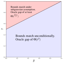
We should also note that stronger upper bounds of the form $h_{t}(\nicefrac{{1}}{{4k}})\leq\exp(-\lambda_{0}t)$ can be found for some $\lambda_{0}>0$ if we assume that the estimators proposed in Theorem 2 are used in stages 0 through $t-1$. This would then make the same class of estimators order-optimal at stage $t$ for every $i\geq 0$. However, proving this relies on the fact that these estimates are subgaussian, and we would not be able to proceed if the estimates chosen in the previous stages have heavier than gaussian tails (but order-optimal error). The two regimes for $\beta,\gamma\in[0,1]^{2}$ are depicted in Figure 2.

Refer to caption
Figure 2: Regimes of minimax loss with $\Theta(t^{\beta})$ real and $\Theta(t^{\beta+\gamma})$ synthetic samples at stage $t$; gaps indicated are w.r.t. the oracle-assisted loss

IV-C2 Data replacement

Consider the data replacement setting where, at every stage $t$, the estimator only has access to samples generated in the current stage $X_{t}^{n}$. Note that $\alpha$ and $n$ do not change with $t$ in this setting, except at stage 0 where all $n$ samples are real.

Let the worst-case expected $\ell_{2}^{2}$ loss at stage $t$ be denoted as $\bar{\sigma}_{t}^{2}$, and define $M:=\sup_{t\geq 0}\bar{\sigma}_{t}^{2}$. Corollary 3, along with Chebyshev’s inequality then gives

$\displaystyle m:=\inf_{t\geq 1}\bar{\sigma}_{t}^{2}\geq\frac{1}{512\left(n\alpha^{2}+M\cdot 16n\alpha k^{2}\right)}.$

When $k$ is fixed, we find that since $M\leq\sqrt{2}$ trivially, $m\geq\nicefrac{{c}}{{n\alpha}}$ for some $c\geq 0$. This is especially stark in contrast to the oracle-assisted infimum, which, with probability $1$, is proportional to $\nicefrac{{1}}{{n}}$, corresponding to the case where all samples are real.

V Proofs

V-A Proofs of the minimax lower bounds

We assume that the alphabet size $k$ is even. The worst-case loss for odd $k$ is lower bounded by the worst-case loss for $k-1$, since the supremum is over a smaller set of distributions.

The lower bound argument uses Assouad’s method with the following construction, widely known in the distribution estimation literature e.g. as described in [11, 12, 13]. Consider the set of vectors $\mathcal{V}=\{+1,-1\}^{k/2}$. With each vector $v\in\mathcal{V}$, associate the distribution

$\displaystyle p_{v}:=p_{u}+\frac{\delta}{k}\begin{bmatrix}v\\ -v\end{bmatrix}$

where $p_{u}$ is the uniform distribution. Let $\mathcal{P}_{k}:=\{p_{v}:v\in\mathcal{V}\}$.

Assouad’s method leads to the lower bound described in the following Lemma. The full proof is provided in Appendix A for completeness.

Lemma 5

The minimax estimation risk described in Definition 2 is lower bounded as

$\displaystyle r^{\ell_{2}^{2}}_{t,k}\geq\frac{\delta^{2}}{4k}\left(1{-}\sqrt{\frac{2}{k}\sum_{j=1}^{k/2}\max_{\begin{subarray}{c}v\in\mathcal{V}:\\ v_{j}=1\end{subarray}}D\Big{(}\bar{\mathbf{P}}_{t,(p_{v})}\Big{\|}\bar{\mathbf{P}}_{t,(p_{v-2e_{j}})}\Big{)}}\right)$ (9)
$\displaystyle r^{\ell_{1}}_{t,k}\geq\frac{\delta}{4}\left(1-\sqrt{\frac{2}{k}\sum_{j=1}^{k/2}\max_{\begin{subarray}{c}v\in\mathcal{V}:\\ v_{j}=1\end{subarray}}D\Big{(}\bar{\mathbf{P}}_{t,(p_{v})}\Big{\|}\bar{\mathbf{P}}_{t,(p_{v-2e_{j}})}\Big{)}}\right)$ (10)

The following Lemma will be useful in the proof of the Theorem:

Lemma 6

Let $Z\sim Q$ be a non-negative random variable and $a$, $b$, and $c$ be some positive constants. Then

$\displaystyle E_{Q}\left[\frac{1}{a+bZ}\right]\leq\frac{Q\{Z<c\}}{a}+\frac{1}{a+bc}.$

We will now prove Theorem 1 by deriving an upper bound on the KL divergences between the distributions $\bar{\mathbf{P}}_{t,(p_{v})}$ and $\bar{\mathbf{P}}_{t,(p_{v-2e_{j}})}$ for each $v\in\mathcal{V}$.

Proof:

Using the chain rule for KL divergences, whenever $j\leq\nicefrac{{k}}{{2}},v[j]=+1$,

$\displaystyle D\Big{(}\bar{\mathbf{P}}_{t,(p_{v})}\Big{\|}\bar{\mathbf{P}}_{t,(p_{v-2e_{j}})}\Big{)}=$ $\displaystyle n_{0}D\left(p_{v}\|p_{v-2e_{j}}\right)+\sum_{i=0}^{t-1}D\left(\left(\tilde{P}({p_{v},\hat{P}_{i},\alpha_{i+1}})\right)^{n_{i+1}}\middle\|\left(\tilde{P}({p_{v-2e_{j}},\hat{P}_{i},\alpha_{i+1}})\right)^{n_{i+1}}\middle|\bar{\mathbf{P}}_{i,(p_{v})}\right)$
$\displaystyle=$ $\displaystyle n_{0}D\left(p_{v}\|p_{v-2e_{j}}\right)$
$\displaystyle\quad+\sum_{i=1}^{t}n_{i}E_{\bar{\mathbf{P}}_{i-1,(p_{v})}}\left[\sum_{j^{\prime}=1}^{k}\left(\alpha_{i}p_{v}[j^{\prime}]+(1-\alpha_{i})\hat{P}_{i-1}[j^{\prime}]\right)\log\frac{\alpha_{i}p_{v}[j^{\prime}]+(1-\alpha_{i})\hat{P}_{i-1}[j^{\prime}]}{\alpha_{i}p_{v-2e_{j}}[j^{\prime}]+(1-\alpha_{i})\hat{P}_{i-1}[j^{\prime}]}\right]$
$\displaystyle\overset{(a)}{\leq}$ $\displaystyle n_{0}\sum_{j^{\prime}=1}^{k}p_{v}[j^{\prime}]\frac{p_{v}[j^{\prime}]-p_{v-2ej}[j^{\prime}]}{p_{v-2ej}[j^{\prime}]}$
$\displaystyle+\sum_{i=1}^{t}n_{i}E_{\bar{\mathbf{P}}_{i-1,(p_{v})}}\left[\sum_{j^{\prime}=1}^{k}\left(\alpha_{i}p_{v}[j^{\prime}]+(1-\alpha_{i})\hat{P}_{i-1}[j^{\prime}]\right)\frac{\alpha_{i}\left(p_{v}[j^{\prime}]-p_{v-2ej}[j^{\prime}]\right)}{\alpha_{i}p_{v-2e_{j}}[j^{\prime}]+(1-\alpha_{i})\hat{P}_{i-1}[j^{\prime}]}\right]$
$\displaystyle=$ $\displaystyle n_{0}\frac{2\delta}{k}\left(\frac{p_{v}[j]}{p_{v-2e_{j}}[j]}-\frac{p_{v}\left[j+\nicefrac{{k}}{{2}}\right]}{p_{v-2e_{j}}\left[j+\nicefrac{{k}}{{2}}\right]}\right)$
$\displaystyle+\sum_{i=1}^{t}n_{i}\left(\frac{2\alpha_{i}\delta}{k}\right)E_{\bar{\mathbf{P}}_{i-1,(p_{v})}}\Bigg{[}\frac{\alpha_{i}p_{v}[j]+(1-\alpha_{i})\hat{P}_{i-1}[j]}{\alpha_{i}p_{v-2e_{j}}[j]+(1-\alpha_{i})\hat{P}_{i-1}[j]}-1$
$\displaystyle\hskip 125.19194pt+1-\frac{\alpha_{i}p_{v}\left[j+\frac{k}{2}\right]+(1-\alpha_{i})\hat{P}_{i-1}\left[j+\frac{k}{2}\right]}{\alpha_{i}p_{v-2e_{j}}\left[j+\frac{k}{2}\right]+(1-\alpha_{i})\hat{P}_{i-1}\left[j+\frac{k}{2}\right]}\Bigg{]}$
$\displaystyle=$ $\displaystyle n_{0}\frac{8\delta^{2}}{k(1-\delta^{2})}+\sum_{i=1}^{t}n_{i}\left(\frac{2\alpha_{i}\delta}{k}\right)^{2}E_{\bar{\mathbf{P}}_{i-1,(p_{v})}}\Bigg{[}\frac{1}{\frac{\alpha_{i}(1-\delta)}{k}+(1-\alpha_{i})\hat{P}_{i-1}[j]}$
$\displaystyle\hskip 184.9429pt+\frac{1}{\frac{\alpha_{i}(1+\delta)}{k}+(1-\alpha_{i})\hat{P}_{i-1}\left[j+\nicefrac{{k}}{{2}}\right]}\Bigg{]},$ (11)

where $(a)$ is a consequence of $\log x\leq x-1$. Recall that $g_{0}(\nicefrac{{1}}{{4k}})=0$ and $\bar{\mathbf{P}}_{i-1,(p_{v})}\left\{\hat{P}_{i-1}[j^{\prime}]<p_{v}[j^{\prime}]-\nicefrac{{1}}{{4k}}\right\}\leq g_{i}(\nicefrac{{1}}{{4k}})$ for every $j^{\prime}\in[1:k]$. Applying Lemma 6 reduces (11) to

$\displaystyle D\Big{(}\bar{\mathbf{P}}_{t,(p_{v})}\Big{\|}\bar{\mathbf{P}}_{t,(p_{v-2e_{i}})}\Big{)}$
$\displaystyle\leq n_{0}\frac{8\delta^{2}}{k(1-\delta^{2})}+\sum_{i=1}^{t}n_{i}\left(\frac{2\alpha_{i}\delta}{k}\right)^{2}\Bigg{(}\frac{1}{\alpha_{i}\frac{1-\delta}{k}+(1-\alpha_{i})\left(\frac{1+\delta}{k}-\frac{1}{4k}\right)}+\frac{\bar{\mathbf{P}}_{i-1,(p_{v})}\left\{\hat{P}_{i-1}[j]<\frac{1+\delta}{k}-\frac{1}{4k}\right\}}{\alpha_{i}\frac{1-\delta}{k}}$
$\displaystyle\hskip 156.49014pt+\frac{1}{\alpha_{i}\frac{1+\delta}{k}+(1-\alpha_{i})\left(\frac{1-\delta}{k}-\frac{1}{4k}\right)}+\frac{\bar{\mathbf{P}}_{i-1,(p_{v})}\left\{\hat{P}_{i-1}\left[j+\frac{k}{2}\right]<\frac{1-\delta}{k}-\frac{1}{4k}\right\}}{\alpha_{i}\frac{1+\delta}{k}}\Bigg{)}$
$\displaystyle\leq n_{0}\frac{8\delta^{2}}{k(1-\delta^{2})}+\sum_{i=1}^{t}n_{i}\frac{(2\alpha_{i}\delta)^{2}}{k}\Bigg{(}\frac{1}{\alpha_{i}({1-\delta})+(1-\alpha_{i})\left(\frac{3}{4}+\delta\right)}+\frac{g_{i}(\nicefrac{{1}}{{4k}})}{\alpha_{i}({1-\delta})}+\frac{1}{\alpha_{i}(1+\delta)+(1-\alpha_{i})\left(\frac{3}{4}-\delta\right)}+\frac{g_{i}(\nicefrac{{1}}{{4k}})}{\alpha_{i}(1+\delta)}\Bigg{)}.$

Now, note that

$\displaystyle\frac{1}{\alpha_{i}(1-\delta)+(1-\alpha_{i})\left(\frac{3}{4}+\delta\right)}+\frac{1}{\alpha_{i}(1+\delta)+(1-\alpha_{i})\left(\frac{3}{4}-\delta\right)}=$ $\displaystyle\frac{2a_{i}}{a_{i}^{2}-b_{i}^{2}\delta^{2}}\leq\frac{2}{\frac{9}{16}-\delta^{2}},$

where $a_{i}:=\nicefrac{{3}}{{4}}(1-\alpha_{i})+\alpha_{i}$ and $b_{i}:=1-2\alpha_{i}$. The inequality holds since $a_{i}\in[\nicefrac{{3}}{{4}},1]$ and $b_{i}\in[-1,1]$. Thus, we finally get

$\displaystyle D\Big{(}\bar{\mathbf{P}}_{t,(p_{v})}\Big{\|}\bar{\mathbf{P}}_{t,(p_{v-2e_{i}})}\Big{)}\leq\frac{8\delta^{2}\sum_{i=0}^{t}n_{i}\alpha_{i}^{2}+n_{i}\alpha_{i}g_{i}(\nicefrac{{1}}{{4k}})}{k\left(\frac{9}{16}-\delta^{2}\right)}.$ (12)

Assuming $\sum_{i=1}^{t}n_{i}\alpha_{i}(\alpha_{i}+g_{i}(\nicefrac{{1}}{{4k}}))\geq\nicefrac{{k}}{{4}}$ and choosing

$\displaystyle\delta^{2}=\frac{k}{64\sum_{i=0}^{t}n_{i}\alpha_{i}(\alpha_{i}+g_{i}(\nicefrac{{1}}{{4k}}))}<1$ (13)

ensures that $D\left(\bar{\mathbf{P}}_{t,(p_{v})}\middle\|\bar{\mathbf{P}}_{t,(p_{v-2e_{j}})}\right)\leq\nicefrac{{1}}{{2}}$. Using Lemma 5 and substituting (13) and (12) into (9) and (10) concludes the proof. ∎

Proof:

A slightly modified version of Lemma 5 leads to the same lower bounds as (9), (10), but with the KL divergence term $D\Big{(}E_{Q_{p_{v}}}\left[\tilde{P}({p_{v},\hat{P},\alpha})\right]\Big{\|}\ E_{Q_{p_{v}}}\left[\tilde{P}({p_{v-2e_{j}},\hat{P},\alpha})\right]\Big{)}$ instead, which has the upper bound

$\displaystyle D\Big{(}E_{Q_{p_{v}}}$ $\displaystyle[\tilde{P}({p_{v},\hat{P},\alpha})]\Big{\|}\ E_{Q_{p_{v}}}[\tilde{P}({p_{v-2e_{j}},\hat{P},\alpha})]\Big{)}\leq E_{Q_{p_{v}}}\left[D\left(\tilde{P}({p_{v},\hat{P},\alpha})\Big{\|}\tilde{P}({p_{v-2e_{i}},\hat{P},\alpha})\right)\right].$

Once again using $\log x\leq x-1$ gives an expression analogous to (11); the rest of the proof follows the same steps as the proof of Theorem 1

V-B Proof of the minimax upper bound

In this section, we derive an upper bound on the minimax expected loss at the $t^{\mathrm{th}}$ stage. The sequence of estimators described here is order-optimal with respect to $n_{t}$ and $\alpha_{t}$ in some regimes; finding optimal estimator sequences in other regimes remains an interesting open problem.

Let $\hat{p}_{\mathrm{emp}}(\cdot)$ be the empirical estimator of a given batch of samples. We have the following Lemma:

Lemma 7

Let $\hat{P}_{0}$ be an unbiased estimate of $p$ with a variance of $\eta\cdot p[j](1-p[j])\geq 0$ for each component $j$. Let samples $X_{1}^{n_{1}}\sim\tilde{P}({p,\hat{P}_{0},\alpha})^{n_{1}}$ as described in Definition 1. Then the estimator

$\displaystyle\hat{P}_{1,(\mathrm{cond})}=\hat{p}_{1,(\mathrm{cond})}(X_{1}^{n_{1}}):=\frac{1}{\alpha}\left(\hat{p}_{\mathrm{emp}}(X_{1}^{n_{1}})-(1-\alpha)\hat{P}_{0}\right)$ (14)

is an unbiased estimator of $p$ and satisfies $E\left[\hat{P}_{0}[j]\cdot\hat{P}_{1,(\mathrm{cond})}[j]\right]=p[j]^{2}$ for every $j\in[1:k]$. Additionally, each component $j$ has variance

$\displaystyle E\left[\left(\hat{P}_{1,(\mathrm{cond})}[j]-p[j]\right)^{2}\right]=\frac{p[j](1-p[j])}{n_{1}\alpha^{2}}\left(1-(1-\alpha)^{2}\eta\right).$ (15)

The proof of this Lemma is deferred to Appendix A.

Using elementary calculations, we also have the following Lemma:

Lemma 8

Let $Y_{0},Y_{1}$ be unbiased estimates of a scalar $\theta$ such that $E[Y_{0}Y_{1}]=\theta^{2}$ and $E[(Y_{j}-\theta)^{2}]=\sigma_{j}^{2}$ for $j=0,1$. For $a_{0},a_{1}\in\mathbb{R}$,

$\displaystyle E[(a_{0}Y_{0}+a_{1}Y_{1}-\theta)^{2}]=a_{0}^{2}\sigma_{0}^{2}+a_{1}^{2}\sigma_{1}^{2}+((a_{0}+a_{1})-1)^{2}\theta^{2}.$

Combining Lemmas 7 and 8, we arrive at the following intermediate result:

Lemma 9

Let $\hat{P}_{0}=\hat{p}_{0}(X_{0}^{n_{0}})$ be an unbiased estimate of $p$ with variance $\eta\cdot\left(\sum_{j}p[j](1-p[j])\right)$ for each component $j$. For $X_{1}^{n_{1}}\sim\tilde{P}({p,\hat{P}_{0}[j],\alpha})^{n_{1}}$, there exists an unbiased estimator $\hat{p}_{1}(\cdot)$ such that for $\hat{P}_{1}:=\hat{p}_{1}(X_{0}^{n_{0}},X_{1}^{n_{1}})$, for each component $j$,

$\displaystyle E_{P_{X_{0}^{n_{0}},X_{1}^{n_{1}}}}\left[\left(\hat{P}_{1}[j]-p[j]\right)^{2}\right]\leq\frac{p[j](1-p[j])}{\frac{1}{\eta}+n_{1}\alpha^{2}}.$ (16)

Moreover, the estimate $\hat{P}_{1}$ thus obtained is a valid distribution almost surely if $\alpha-\alpha^{2}\leq\frac{1}{\eta n_{1}}$.

Proof:

Let $\hat{P}_{1}=a_{0}\hat{P}_{0}+a_{1}\hat{P}_{1,(\mathrm{cond})}$ with

$\displaystyle a_{0}=\frac{\nicefrac{{1}}{{\eta}}}{\nicefrac{{1}}{{\eta}}+\nicefrac{{1}}{{(n_{1}\alpha^{2})}}}\mbox{ and }a_{1}=1-a_{0}.$

The resulting estimator can then be expressed as

$\displaystyle\hat{p}_{1}(X_{0}^{n_{0}},X_{1}^{n_{1}})=\hat{p}_{0}(X_{0}^{n_{0}})+\frac{n_{1}\alpha}{\frac{1}{\eta}+n_{1}\alpha^{2}}\left(\hat{p}_{\mathrm{emp}}(X_{1}^{n_{1}})-\hat{p}_{0}(X_{0}^{n_{0}})\right).$ (17)

Now, $\alpha-\alpha^{2}\leq\frac{1}{\eta n_{1}}$ ensures that the RHS of (17) is a convex combination of two distributions in $\Delta_{k}$, thus ensuring that $\hat{P}^{(1)}$ is a valid distribution almost surely. Using Lemmas 7 and 8 leads to the desired upper bound on the componentwise variances. ∎

Proof:

If $\hat{p}_{0}$ is the empirical estimator, it is well known that $E[\ell_{2}^{2}(\hat{P}_{0}[j],p[j])]=\nicefrac{{p[j](1-p[j])}}{{n_{0}}}$. Proceeding inductively and repeatedly applying Lemma 9, we find that the estimated distribution at each stage $t$ has mean $p$, and thus the expected $\ell_{2}^{2}$ loss is precisely the sum of the componentwise variances, each bounded above as

$\displaystyle E\left[\left(\hat{P}_{t}[j]-p[j]\right)^{2}\right]\leq\frac{p[j](1-p[j])}{\sum_{i=0}^{t}n_{i}\alpha_{i}^{2}}.$

Noting that the estimate found at stage $t$ is a valid distribution if $n_{t}\alpha_{t}-n_{t}\alpha_{t}^{2}\leq\sum_{i=0}^{t-1}n_{i}\alpha_{i}^{2}$ (from the condition in Lemma 9) and $\sum_{j}p[j](1-p[j])\leq 1-\nicefrac{{1}}{{k}}$ leads to result for the $\ell_{2}^{2}$ loss. Using the Cauchy-Schwarz inequality leads to the upper bound on the $\ell_{1}$ loss. ∎

Appendix A Proofs of Auxiliary Lemmas

In this section, we present complete proofs for the Lemmas and results used in Section V.

Proof:

We first prove the lemma for the $\ell_{2}^{2}$ loss. Define the sign$(.)$ function as

$\displaystyle\mathrm{sign}(x)=\begin{cases}-1&x<0\\ 0&x=0\\ 1&x>0.\end{cases}$

and let $\mathds{1}\{.\}$ be the indicator function.

$\displaystyle\sup_{p\in\Delta_{k}}E_{\bar{\mathbf{P}}_{t,(p)}}[l_{2}^{2}(\hat{P}_{t},p)]\geq$ $\displaystyle\sup_{p\in\mathcal{P}_{k}}E_{\bar{\mathbf{P}}_{t,(p)}}[l_{2}^{2}(\hat{P}_{t},p)]$
$\displaystyle\geq$ $\displaystyle\sup_{v\in\mathcal{V}}E_{\bar{\mathbf{P}}_{t,(p_{v})}}\left[\sum_{j=1}^{k/2}\left(\hat{P}_{t}-\frac{1}{k}-v_{j}\frac{\delta}{k}\right)^{2}\right]$ (18)
$\displaystyle\geq$ $\displaystyle\frac{\delta^{2}}{k^{2}}\sup_{v\in\mathcal{V}}E_{\bar{\mathbf{P}}_{t,(p_{v})}}\left[\sum_{j=1}^{k/2}\mathds{1}\left\{\mathrm{sign}\left(\hat{P}_{t}-\frac{1}{k}\right)\neq v_{j}\right\}\right]$ (19)
$\displaystyle\geq$ $\displaystyle\frac{\delta^{2}}{k^{2}}\sum_{v\in\mathcal{V}}\frac{1}{|\mathcal{V}|}\sum_{j=1}^{k/2}E_{\bar{\mathbf{P}}_{t,(p_{v})}}\left[\mathds{1}\left\{\mathrm{sign}\left(\hat{P}_{t}-\frac{1}{k}\right)\neq v_{j}\right\}\right]$
$\displaystyle=$ $\displaystyle\frac{\delta^{2}}{k^{2}}\sum_{j=1}^{k/2}\frac{1}{|\mathcal{V}|}\sum_{v\in\mathcal{V}}E_{\bar{\mathbf{P}}_{t,(p_{v})}}\left[\mathds{1}\left\{\mathrm{sign}\left(\hat{P}_{t}-\frac{1}{k}\right)\neq v_{j}\right\}\right]$ (20)

Let $\mathcal{V}_{+j}=\{v\in\mathcal{V}:v_{j}=+1\}$ and $\mathcal{V}_{-j}=\{v\in\mathcal{V}:v_{j}=-1\}$. Note that these are sets of equal size, and their union is $\mathcal{V}$. Denote the mixtures $\frac{1}{|\mathcal{V}_{+j}|}\sum_{v\in\mathcal{V}_{+j}}\bar{\mathbf{P}}_{t,(p_{v})}$ and $\frac{1}{|\mathcal{V}_{-j}|}\sum_{v\in\mathcal{V}_{-j}}\bar{\mathbf{P}}_{t,(p_{v})}$ as $\bar{\mathbf{Q}}_{t,(+j)}$ and $\bar{\mathbf{Q}}_{t,(-j)}$ respectively. Rewriting (20) using $E_{Q}[\mathds{1}\{A\}]=Q(A)$,

$\displaystyle r^{l_{2}^{2}}_{\lambda,n_{0},n_{1}}\geq$ $\displaystyle\frac{\delta^{2}}{k^{2}}\sum_{j=1}^{k/2}\frac{1}{2}\Bigg{[}\bar{\mathbf{Q}}_{t,(+j)}\left(\mathrm{sign}\left(\hat{P}_{t}-\frac{1}{k}\right)=-1\right)$
$\displaystyle\qquad\qquad+\bar{\mathbf{Q}}_{t,(-j)}\left(\mathrm{sign}\left(\hat{P}_{t}-\frac{1}{k}\right)=+1\right)\Bigg{]}$
$\displaystyle=$ $\displaystyle\frac{\delta^{2}}{2k^{2}}\sum_{j=1}^{k/2}\Bigg{[}1-\bar{\mathbf{Q}}_{t,(+j)}\left(\mathrm{sign}\left(\hat{P}_{t}-\frac{1}{k}\right)=+1\right)$
$\displaystyle\qquad\qquad+\bar{\mathbf{Q}}_{t,(-j)}\left(\mathrm{sign}\left(\hat{P}_{t}-\frac{1}{k}\right)=+1\right)\Bigg{]}$
$\displaystyle\geq$ $\displaystyle\frac{\delta^{2}}{2k^{2}}\sum_{j=1}^{k/2}\left[1-\sup_{A\subset\mathcal{X}^{n_{0}+n_{1}}}\left(\bar{\mathbf{Q}}_{t,(+j)}(A)-\bar{\mathbf{Q}}_{t,(-j)}(A)\right)\right]$
$\displaystyle=$ $\displaystyle\frac{\delta^{2}}{2k^{2}}\sum_{j=1}^{k/2}\left[1-\|\bar{\mathbf{Q}}_{t,(+j)}-\bar{\mathbf{Q}}_{t,(-j)}\|_{\mathrm{TV}}\right]$
$\displaystyle\overset{(a)}{\geq}$ $\displaystyle\frac{\delta^{2}}{2k^{2}}\sum_{j=1}^{k/2}\left[1-\frac{2}{|\mathcal{V}|}\sum_{\begin{subarray}{c}v\in\mathcal{V}:\\ v_{j}=1\end{subarray}}\|\bar{\mathbf{P}}_{t,(p_{v})}-\bar{\mathbf{P}}_{t,(p_{v-2e_{j}})}\|_{\mathrm{TV}}\right]$
$\displaystyle\geq$ $\displaystyle\frac{\delta^{2}}{2k^{2}}\sum_{j=1}^{k/2}\left[1-\max_{\begin{subarray}{c}v\in\mathcal{V}:\\ v_{j}=1\end{subarray}}\|\bar{\mathbf{P}}_{t,(p_{v})}-\bar{\mathbf{P}}_{t,(p_{v-2e_{j}})}\|_{\mathrm{TV}}\right]$
$\displaystyle\geq$ $\displaystyle\frac{\delta^{2}}{4k}\left(1-\frac{2}{k}\sum_{j=1}^{k/2}\max_{\begin{subarray}{c}v\in\mathcal{V}:\\ v_{j}=1\end{subarray}}\|\bar{\mathbf{P}}_{t,(p_{v})}-\bar{\mathbf{P}}_{t,(p_{v-2e_{j}})}\|_{\mathrm{TV}}\right)$
$\displaystyle\overset{(b)}{\geq}$ $\displaystyle\frac{\delta^{2}}{4k}\left(1-\sqrt{\frac{2}{k}\sum_{j=1}^{k/2}\max_{\begin{subarray}{c}v\in\mathcal{V}:\\ v_{j}=1\end{subarray}}\|\bar{\mathbf{P}}_{t,(p_{v})}-\bar{\mathbf{P}}_{t,(p_{v-2e_{j}})}\|_{\mathrm{TV}}^{2}}\right)$
$\displaystyle\overset{(c)}{\geq}$ $\displaystyle\frac{\delta^{2}}{4k}\left(1-\sqrt{\frac{2}{k}\sum_{j=1}^{k/2}\max_{\begin{subarray}{c}v\in\mathcal{V}:\\ v_{j}=1\end{subarray}}D_{KL}\left(\bar{\mathbf{P}}_{t,(p_{v})}\|\bar{\mathbf{P}}_{t,(p_{v-2e_{j}})}\right)}\right)$ (21)

where $(a)$ is due to Jensen’s inequality, $(b)$ is due to the Cauchy-Schwarz inequality, and $(c)$ is due to Pinsker’s inequality. The result for the $\ell_{1}$ loss follows directly by observing that for the $\ell_{1}$ loss, the inequality (18) holds with absolute values in the expectation instead of squares, and the equivalent penalty in (19) is $\nicefrac{{\delta}}{{k}}$ instead of $\nicefrac{{\delta^{2}}}{{k^{2}}}$; the rest of the analysis follows exactly the same steps. ∎

Proof:

First, note that the empirical estimator is the normalized sum of indicator random variables of the form

$\displaystyle\hat{p}_{\mathrm{emp}}(X_{1}^{n_{1}})[j]=\frac{\sum_{s=1}^{n_{1}}\mathds{1}\{X_{1}[s]=j\}}{n_{1}}.$

Conditioned on $\hat{P}_{0}[j]$, each of these indicator random variables is distributed as $\mathrm{Bern}\left(\alpha p[j]+(1-\alpha)\hat{P}_{0}[j]\right)$ independently of the others. If $\hat{P}_{0}$ is an unbiased estimate, then $E[\hat{p}_{\mathrm{emp}}(X_{1}^{n_{1}})]=E[E[\hat{p}_{\mathrm{emp}}(X_{1}^{n_{1}})|\hat{P}_{0}]]=E[\alpha\hat{P}_{0}+(1-\alpha)p]=p$, and therefore, $\hat{p}_{\mathrm{emp}}(X_{1}^{n_{1}})$ is an unbiased estimate of $p$.

Consequently, since the sum of the coefficients of $\hat{p}_{\mathrm{emp}}$ and $\hat{P}_{1}$ in (14) is $1$, $\hat{P}_{1,(\mathrm{cond})}$ is also an unbiased estimate of $p$. Also,

$\displaystyle E\left[\hat{P}_{0}[j]\hat{P}_{1,(\mathrm{cond})}[j]\right]=$ $\displaystyle E\left[E\left[\hat{P}_{0}[j]\hat{P}_{1,(\mathrm{cond})}[j]\middle|\hat{P}_{0}[j]\right]\right]$
$\displaystyle=$ $\displaystyle E\left[\frac{\hat{P}_{0}[j]}{\alpha}\left(\alpha p[j]+(1-\alpha)\hat{P}_{0}[j]-(1-\alpha)\hat{P}_{0}[j]\right)\right]$
$\displaystyle=$ $\displaystyle E\left[p[j]\hat{P}_{0}[j]\right]=p[j]^{2}.$

This concludes the proof of the first two parts of the Lemma. We now compute the variance of the estimator $\hat{P}_{1,(\mathrm{cond})}$. The variance of $\hat{P}_{\mathrm{emp}}[j]:=\hat{p}_{\mathrm{emp}}(X_{1}^{n_{1}})[j]$ is

$\displaystyle E\left[\left(\hat{P}_{\mathrm{emp}}[j]-p[j]\right)^{2}\right]=$ $\displaystyle E\left[(\hat{P}_{\mathrm{emp}}[j])^{2}\right]-p[j]^{2}$
$\displaystyle=$ $\displaystyle E\left[E\left[\left(\hat{P}_{\mathrm{emp}}[j]\right)^{2}\middle|\hat{P}_{0}[j]\right]\right]-p[j]^{2}$
$\displaystyle=$ $\displaystyle E\left[\left(\alpha p[j]+(1-\alpha)\hat{P}_{0}[j]\right)^{2}\left(1-\frac{1}{n_{1}}\right)+\frac{1}{n_{1}}\left(\alpha p[j]+(1-\alpha)\hat{P}_{0}[j]\right)\right]-p[j]^{2}$
$\displaystyle=$ $\displaystyle(1-\alpha)^{2}\left(1-\frac{1}{n_{1}}\right)E\left[\left(\hat{P}_{0}[j]-p[j]\right)^{2}\right]+\frac{p[j]-p[j]^{2}}{n_{1}}$
$\displaystyle=$ $\displaystyle(1-\alpha)^{2}\left(1-\frac{1}{n_{1}}\right)\eta\cdot p[j]\left(1-p[j]\right)+\frac{p[j](1-p[j])}{n_{1}}.$
$\displaystyle=$ $\displaystyle p[j](1-p[j])\left(\frac{1}{n_{1}}+\eta(1-\alpha)^{2}\left(1-\frac{1}{n_{1}}\right)\right).$ (22)

The covariance of $\hat{P}_{\mathrm{emp}}$ and $\hat{P}_{0}$ is

$\displaystyle E\left[\hat{P}_{\mathrm{emp}}[j]\hat{P}_{0}[j]\right]-p[j]^{2}=$ $\displaystyle E\left[E\left[\hat{P}_{\mathrm{emp}}[j]\hat{P}_{0}[j]\big{|}\hat{P}_{0}[j]\right]\right]-p[j]^{2}$
$\displaystyle=$ $\displaystyle E\left[\left(\alpha p[j]+(1-\alpha)\hat{P}_{0}[j]\right)\hat{P}_{0}[j]\right]-p[j]^{2}$
$\displaystyle=$ $\displaystyle\alpha p[j]^{2}+(1-\alpha)E\left[\left(\hat{P}_{0}[j]\right)^{2}\right]-p[j]^{2}$
$\displaystyle=$ $\displaystyle(1-\alpha)\left(E\left[\left(\hat{P}_{0}[j]\right)^{2}\right]-p[j]^{2}\right)$
$\displaystyle=$ $\displaystyle(1-\alpha)\eta\cdot p[j]\left(1-p[j]\right).$ (23)

Using (22) and (23), the variance of $\hat{P}_{1,(\mathrm{cond})}[j]$ is then

$\displaystyle E\left[\left(\hat{P}_{1,(\mathrm{cond})}[j]-p[j]\right)^{2}\right]=$ $\displaystyle\frac{1}{\alpha^{2}}\left(\text{var}\left(\hat{P}_{\mathrm{emp}}[j]\right)+(1-\alpha)^{2}\text{var}\left(\hat{P}_{0}[j]\right)-2(1-\alpha)\text{cov}\left(\hat{P}_{0}[j],\hat{P}_{\mathrm{emp}}[j]\right)\right)$
$\displaystyle=$ $\displaystyle\frac{p[j]\left(1-p[j]\right)}{\alpha^{2}}\left(\frac{1}{n_{1}}+\eta(1-\alpha)^{2}\left(1-\frac{1}{n_{1}}\right)+(1-\alpha)^{2}\cdot\eta-2\eta(1-\alpha)^{2}\right)$
$\displaystyle=$ $\displaystyle\frac{p[j]\left(1-p[j]\right)}{n_{1}\alpha^{2}}\left(1-\eta(1-\alpha)^{2}\right).$

References

  • [1] S. Kamath, A. Orlitsky, D. Pichapati, and A. T. Suresh, “On Learning Distributions from their Samples,” in Proceedings of The 28th Conference on Learning Theory, pp. 1066–1100, PMLR, June 2015.
  • [2] S.-O. Chan, I. Diakonikolas, X. Sun, and R. A. Servedio, “Learning mixtures of structured distributions over discrete domains,” in Proceedings of the 2013 Annual ACM-SIAM Symposium on Discrete Algorithms (SODA), Proceedings, pp. 1380–1394, Society for Industrial and Applied Mathematics, Jan. 2013.
  • [3] Y. Han, J. Jiao, and T. Weissman, “Minimax minimax estimation of discrete distributions under $\ell_{1}$ loss,” IEEE Transactions on Information Theory, vol. 61, pp. 6343–6354, Nov. 2015.
  • [4] A. Mahadevan, “This newspaper doesn’t exist: How ChatGPT can launch fake news sites in minutes.” https://www.poynter.org/fact-checking/2023/chatgpt-build-fake-news-organization-website/, Feb. 2023.
  • [5] I. Shumailov, Z. Shumaylov, Y. Zhao, N. Papernot, R. Anderson, and Y. Gal, “AI models collapse when trained on recursively generated data,” Nature, vol. 631, pp. 755–759, July 2024. First published at arXiv:2305.17493.
  • [6] S. Alemohammad, J. Casco-Rodriguez, L. Luzi, A. I. Humayun, H. Babaei, D. LeJeune, A. Siahkoohi, and R. G. Baraniuk, “Self-Consuming Generative Models Go MAD,” July 2023. arXiv:2307.01850.
  • [7] Q. Bertrand, J. Bose, A. Duplessis, M. Jiralerspong, and G. Gidel, “On the stability of iterative retraining of generative models on their own data,” in The Twelfth International Conference on Learning Representations, 2024. First published at arXiv:2310.00429.
  • [8] S. Fu, S. Zhang, Y. Wang, X. Tian, and D. Tao, “Towards theoretical understandings of self-consuming generative models,” in Forty-first International Conference on Machine Learning, 2024. First published at arXiv:2402.11778.
  • [9] E. Dohmatob, Y. Feng, and J. Kempe, “Model collapse demystified: The case of regression,” in The Thirty-eighth Annual Conference on Neural Information Processing Systems, 2024. First published at arXiv:2402.07712.
  • [10] M. Gerstgrasser, R. Schaeffer, A. Dey, R. Rafailov, T. Korbak, H. Sleight, R. Agrawal, J. Hughes, D. B. Pai, A. Gromov, D. Roberts, D. Yang, D. L. Donoho, and S. Koyejo, “Is model collapse inevitable? breaking the curse of recursion by accumulating real and synthetic data,” in First Conference on Language Modeling, 2024. First published at arXiv:2404.01413.
  • [11] A. B. Tsybakov, Introduction to Nonparametric Estimation. Springer Series in Statistics, New York, NY: Springer, 2009.
  • [12] B. Yu, “Assouad, Fano, and Le Cam,” in Festschrift for Lucien Le Cam: Research Papers in Probability and Statistics (D. Pollard, E. Torgersen, and G. L. Yang, eds.), pp. 423–435, New York, NY: Springer, 1997.
  • [13] Y. Polyanskiy and Y. Wu, Information theory: From coding to learning. Cambridge university press, 2024.