[1]Scuola Superiore Meridionale, Largo S. Marcellino 10, 80138 Napoli, Italy \affil[2]Istituto Nazionale di Fisica Nucleare (INFN) Sezione di Napoli \affil[3]Università degli Studi di Napoli Federico II , Dipartimento di Fisica Ettore Pancini \affil[4]Department of Physics and Astronomy, University of Southern California, Los Angeles, USA
Entanglement and Stabilizer entropies of random bipartite pure quantum states
Abstract
The interplay between non-stabilizerness and entanglement in random states is a very rich arena of study for the understanding of quantum advantage and complexity. In this work, we tackle the problem of such interplay in random pure quantum states. We show that while there is a strong dependence between entanglement and magic, they are, surprisingly, perfectly uncorrelated. We compute the expectation value of non-stabilizerness given the Schmidt spectrum (and thus entanglement). At a first approximation, entanglement determines the average magic on the Schmidt orbit. However, there is a finer structure in the average magic distinguishing different orbits where the flatness of entanglement spectrum is involved.
1 Introduction
Entanglement has long been regarded a cornerstone of quantum information science, distinguishing quantum mechanics from classical theories and serving as a pivotal resource for quantum technologies [1]. Since the advent of the stabilizer formalism, it has been clear that entanglement is not enough to provide computational advantage [2]. Such a formalism identifies a set of states, called stabilizer states, which have the peculiar feature of being efficiently simulable using classical computational resources despite being possibly highly entangled [2, 3]. States away from the set of stabilizer states are a fundamental resource for universal quantum computation. Indeed, the distance from the set of the stabilizer states [4] defines the non-stabilizer resource, which also plays an important role in characterizing the complexity of quantum states and processes [5, 6, 7, 8, 9, 10, 11].
Entanglement and magic are thus distinct but interrelated resources for understanding the structure and behavior of quantum states. Previous investigations into this interplay have yielded several key insights. Notably, entanglement can be computed exactly for stabilizer states [12, 13], establishing a foundational link between entanglement and classical simulability. The probability distribution of entanglement in random stabilizer states [14] establishes another connection between entanglement and the free stabilizer resources. A series of works show that this kind of entanglement has a simple pattern [15] and that entanglement complexity arises when enough non-stabilizer resources (also known as magic) are injected [15, 16, 17]. Furthermore, a connection between non-stabilizerness and the entanglement response of quantum systems, i.e. anti-flatness of the reduced density operator, has been identified [18], highlighting how these resources interact under system dynamics. Additionally, a computational phase separation has been observed, categorizing quantum states into two distinct regimes: entanglement-dominated and magic-dominated phases [19].
This work aims at establishing some exact results in the interplay between entanglement and non-stabilizerness in random pure quantum states. We will utilize Stabilizer Entropy (SE) [8] as the unique computable monotone for non-stabilizerness [20]. We start with a simple consideration that has, though, profound consequences: the separable state with maximal SE is much less resourceful than the average pure state drawn from the Haar measure.
Haar-random states are typically highly entangled so we see that most entangled states possess a (much) higher SE than the maximum-SE separable state. This means that entanglement makes room for non-stabilizerness and that the two resources must feature a rich interplay.
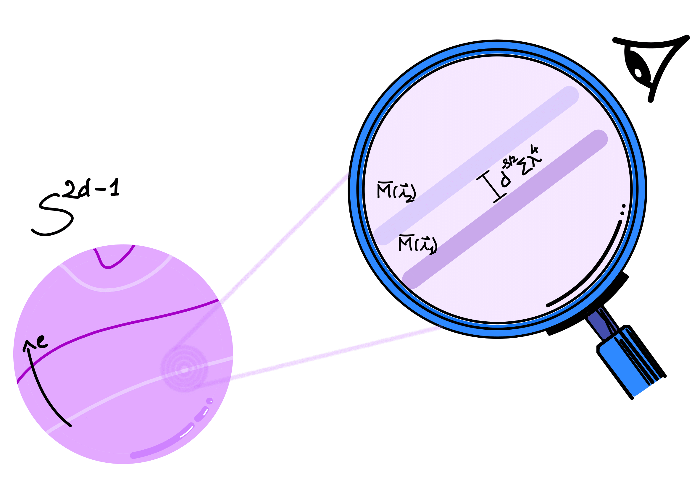
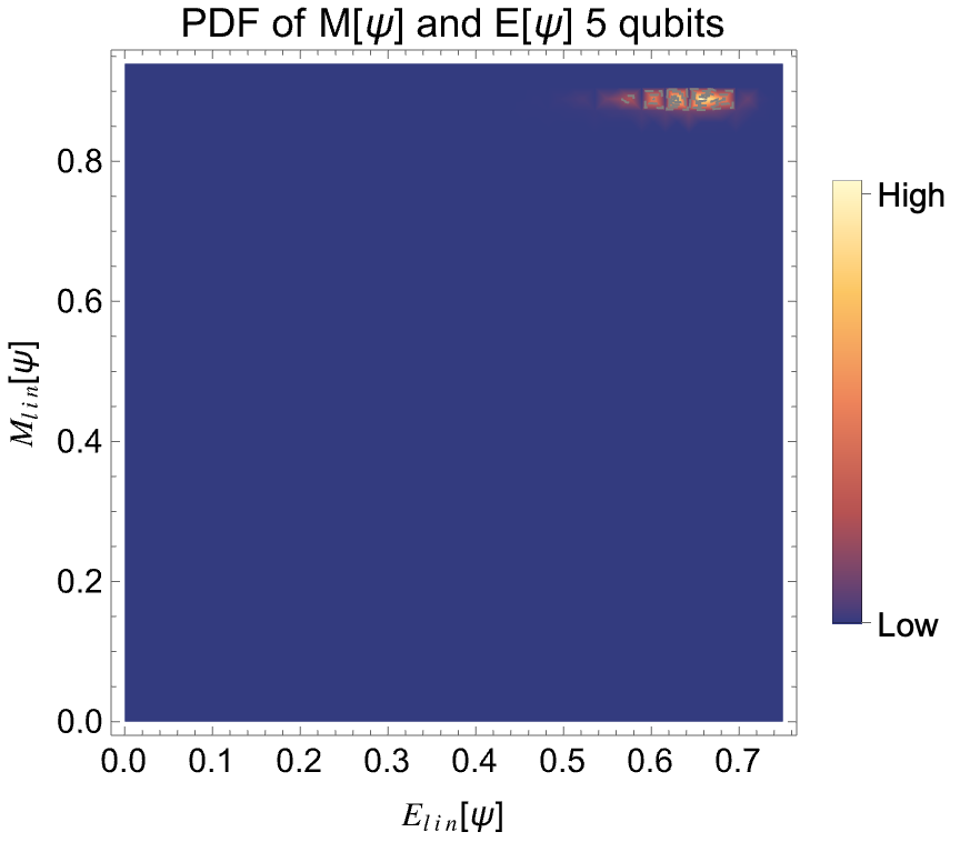
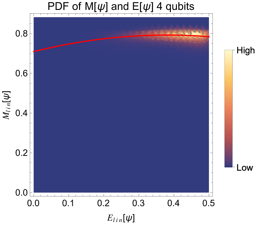
In this paper, we give a quantitative and analytical analysis of the dependence of these two quantities in random pure states. A numerical analysis with similar scope was recently presented in [21]. The main result of this work is the surprising fact that magic and entanglement are exactly uncorrelated (in their linear versions), yet dependent, and a way to picture this intricate dependence is via the foliation of the Hilbert space of bipartite pure states using the concept of Schmidt orbits, see Fig. 1.
The paper is structured as follows: In Section 2 we setup the notation, the necessary tools such as Haar measure and a survey of known results on linear entanglement and SE. Section 3 discusses the surprising results that the linear entanglement and SE have null covariance. In Section 4 we address the dependence between entanglement and SE presenting a calculation of the average SE over Schmidt orbits and present results about its typically. In Section 5 we compute the averaged magic at fixed entanglement for the specific case of a -dimensional bipartite Hilbert space. Finally, Section 6 discusses the broader picture in which the result of the previous section stands in the literature, namely the connection with anti-flatness.
2 Setting the stage
In this section we give a description of the tools and notation used in the paper. We consider a finite dimensional Hilbert space . Concretely is a collection of qubits, i.e. and . Owing to normalization, the set of pure states on can be identified with the hypersphere , more precisely any pure state can be identified with a Hopf circle on the sphere . On this manifold (isomorphic to ) there is a unique, unitarily invariant measure . This measure is induced by the Haar measure on the corresponding unitary group when applied to a fiducial state , i.e.
| (1) |
for any integrable function . A function from the set of pure states to becomes a real random variable when is equipped with this uniform measure. Expectation values of are computed with Eq. (1) via .
2.1 Entanglement and Linear Entanglement Entropy
In this paper we consider two particular functions on the set of pure states quantifying, respectively, entanglement and non-stabilizerness. In order to be more symmetric with respect to our choice of magic measure (see below), we consider the linear entanglement entropy as a measure of entanglement. is defined as
| (2) |
where indicates the pure state and . The linear entanglement entropy is also related to the concurrence via , and to the entanglement 2-Rényi entropy, via .
In order to define the measure of magic that we are going to consider we briefly review some basic facts about the stabilizer formalism.
2.2 Non-stabilizerness and Stabilizer Entropy
The Pauli group on qubits is defined as
| (3) |
In this work, single tensor product of Pauli matrices is referred to as Pauli strings of Pauli operators . Pauli strings play an important role, since they also provide an orthogonal basis for the space of linear operators on . Let us denote the Clifford group as the normalizer of the Pauli group, namely
| (4) |
Given these elements, the set of stabilizer states of is defined as the orbit of the Clifford group through the computational basis states (namely, the eigenstates of the operator): in formulas,
| (5) |
Equivalently, a pure stabilizer state is defined as the common eigenstate of mutually commuting Pauli strings.
Stabilizer states share some properties about the computational complexity of simulating quantum processes using classical resources. These properties are summarized by the Gottesman-Knill theorem, which states that any quantum process that can be represented with initial stabilizer states upon which one performs (i) Clifford unitaries, (ii) measurements of Pauli operators, (iii) Clifford operations conditioned on classical randomness, can be perfectly simulated by a classical computer in polynomial time [2]. Since the set of stabilizer states is by definition closed under Clifford operations, some resources, such as unitary operations outside the Clifford group or states not in , need to be injected in the quantum system in order to make it universal. These non-stabilizer resources, referred to as non-stabilizerness (or magic) of the state, have been proven to be a useful resource for universal quantum computation [22] and several measures have been proposed to quantify it [23, 24]. We will focus on the essentially only computable measure for non-stabilizerness, namely the Stabilizer Entropy (SE) and in particular, the 2-Stabilizer Rényi Entropy [25] and its linear counterpart . Starting from the probability distribution , with , associated to the tomography of the quantum state , the -Stabilizer Rényi Entropy for pure states is defined as
| (6) |
with , whereas the linear SE is defined as follows:
| (7) |
where is the stabilizer purity. Both of these measures are: (i) faithful, i.e. ; (ii) non-increasing over free operations, that is the operations preserving ; (iii) additive (or multiplicative for the stabilizer purity SP) under tensor product, namely . Both the linear and the logarithmic SEs are regarded as good monotones for the pure-state resource theory of stabilizer computation [20]. In this work, the linear version of SE will be implemented, as it is easier to handle in the context of Haar averages.
2.3 Known results about Entanglement and Non-stabilizerness
Now that we defined our measures of entanglement and magic we review some known facts about them when considered independently. The first two moments of and have been computed. In particular one has [26, 27, 28] with )
| (8) |
Since in the region and , , this indicates that on average, except for the case when one of the two dimensions is small, generic states in the Hilbert space are nearly maximally entangled.
The variance of has been computed in [29] and reads
| (9) |
Since the variance tends to zero as , the distribution of becomes increasingly peaked as the dimension grows. Using Chebyshev’s inequality one can show that the probability that is very different from its average value is very small. One says then that typically is close to its average or simply that the random variable is typical.
Another way of proving the typicality of is by use of Lévy’s lemma. In Lemma III.8 of [30] the authors show that the Lipschitz constant of is upper bounded by . Using a similar reasoning or with little modification one can show that the same holds for with Lipschitz constant , hence one can state that entanglement also exhibits the stronger typicality offered by Lévy’s lemma.
Average and variance (corresponding to the first two cumulants) are also known for the linear magic . In this case one has (see [25, 31])
| (10) |
Since also the variance of the magic vanishes when (and with a greater exponent than that of the entanglement), using Chebyshev’s inequality one can prove typicality of . Alternatively, using the Lipshitz constant found in [31] and Levy’s lemma, one can easily obtain that [25]
| (11) |
3 Covariance between Entanglement and Magic
The strongest motivation behind this work is to further understand the relationship between magic and entanglement in random states. The need for clarification of the interplay between magic and entanglement has been fueled by various numerical evidence regarding the maximum achievable value of magic through separable states. The (pure) single-qubit state achieving maximum SE is the so-called golden state, defined as:
| (12) |
We can see then that the separable state with maximal SE is much less resourceful than the average state in the Hilbert space. Since one can show that one has the following bound
| (13) |
and a similar situation holds for , namely
| (14) |
We see that as most states in the Hilbert space are very entangled, entanglement is a precondition to have high - magic states. In other words, this shows that there is a strong interplay between non-stabilizerness and entanglement.
One would be tempted to say, in fact, that and are strongly correlated. We therefore set out to compute the covariance
| (15) |
Surprisingly, we find the following result.
Proposition 1.
The linear entanglement and linear magic, when seen as random variables over the states of pure states equipped with the uniform measure, are uncorrelated. Namely:
| (16) |
In order to prove the above proposition we divided all the 720 permutations of the symmetric group of six elements into conjugacy classes and performed traces over all of them (see Appendix E for details). The same result of lack of covariance does not hold for the non-linearized versions of the variables. However, there is numerical evidence by analysis of Fig. 2 and the numerical analysis on the fluctuations of magic and entanglement in the recent [21] that suggest that the covariance of the logarithmic versions of entanglement and SE tends to zero in the thermodynamic limit.
This fact, although unexpected, does not imply that entanglement and magic are independent as notably independence implies that the variables are uncorrelated but not vice-versa111For a toy example of this phenomenon, consider a standard Gaussian random variable and its square (obviously dependent on ). The covariance between and is equal to the third moment which is obviously zero.. In fact, the covariance detects only the linear dependence between the variables. In order to obtain a better understanding of the dependence between entanglement and magic a more detailed study is required. This will be the content of the next section.
4 Magic conditioned by entanglement and averages over Schmidt orbits
After considering the previous results about the absence of covariance between entanglement and magic, we would like to characterize their dependence. In this section, we examine the average behavior of magic given the non-local properties of the state. To this goal, we fix the Schmidt coefficients in a bipartition and compute the average magic on the Schmidt orbit. In this way, we find some technical results on non-local magic, and thus the average interplay between magic and entanglement.
Two random variables are independent if the realization of one does not affect the probability distribution of the other. The most complete way to quantify the dependence of two random variables is to compute their conditional probabilities, such as , the probability distribution of given that entanglement has the value . The variables are independent if for all values of . In the following, we set out to obtain a partial information regarding this conditional probability, namely its average.
Consider a pure state in the bipartite system . Fixing a product basis in , the pure state is represented by a rectangular matrix . We now perform a singular value decomposition on this matrix, , where are unitaries in and is the rectangular matrix with the singular values, , of on the diagonal. Assuming , this corresponds to the Schmidt decomposition
| (17) |
If is sampled uniformly with the Haar measure, i.e. with Haar distributed, what is the measure induced by the Schmidt decomposition? It turns out that it is a product measure [32]
| (18) |
where the first factor denotes the natural, unitarily invariant distribution on the flag manifold , while the probability distribution on the simplex has been computed in [33, 34, 35, 36]. The quotient with arises because the Schmidt decomposition is invariant under the gauge symmetry where is a diagonal unitary matrix with phases while is has the same phases on the diagonal and zero on the remaining entries.
For the functions we are interested in, functions of and , Haar integration over the flag manifold coincides with Haar integration over and (see Appendix A). Then we have the following result
| (19) |
where is a reference state with given Schmidt coefficients. Moreover, since depends only on the Schmidt coefficients and not on the unitaries , we have
| (20) |
Looking at Eq. (19), we note that we reduced the task to that of computing averages over the Schmidt orbits
| (21) |
This is reminiscent of the approach in [37]. As anticipated, we will content ourselves with the first moment of the above conditional probability, namely
| (22) |
Define now the average magic over Schmidt orbits, , as
| (23) |
then the average magic given entanglement is given by
| (24) |
The average magic over the Schmidt orbit is an interesting quantity on its own right. As we shall see, it is an independent invariant additional to entanglement and reveals a finer structure of these orbits. Then we have the following proposition (see Appendix F for a proof).
Proposition 2.
Given a bipartite -qubit Hilbert space with dimensions , the average value of over the Schmidt orbit on the reference state reads
| (25) |
where
| (26) |
and the normalization implies while the linear entanglement entropy is .
Notice that if is separable reads
| (27) |
whereas for maximally entangled states one has
| (28) |
In the large d limit with , Eq. (25) becomes
| (29) |
As one can see, in the large limit, the leading term (up to ) depends only on the entanglement of the orbit. It seems that at first glance, the average magic of states with a fixed Schmidt decomposition can be approximated by a quadratic polynomial of its entanglement: however, there are dependences on higher moments of the Schmidt distribution that distinguish the orbits. In the region where the asymptotic expansion becomes
| (30) |
hence, even in this case the behavior is similar to that of Eq. (29).
Using Eq. (24) one can readily obtain the leading behavior of the average magic at given entanglement in the above defined regions:
| (31) | ||||
| (32) |
What the above results tell us is that the Schmidt orbits of magic are, at leading order, completely fixed by the entanglement. However, within these orbits, there is a finer structure where higher moments of the Schmidt spectrum are involved and carry information about the anti-flatness of the entanglement spectrum [18, 38], see Fig. 1 for an illustration. These results also describe the non-local character of non-stabilizer resources, as involved, for instance, in the AdS-CFT correspondence [38].
4.1 Typicality of the result
The significance of the result obtained in Eq. (25) is quantified by its typicality. To this end, the Chebyshev inequality is used, and in particular, the Bhatia-Davis [39] inequality is employed to bound the variance of . Such inequality states that, given a bounded random variable ,
| (33) |
Applying this inequality to , which is bounded between and , this inequality reads
| (34) |
direct evaluation of the right-hand side leads to the following bound:
| (35) |
Hence, applying this bound to the Chebyshev inequality one can state that
| (36) |
Given that , deviations can never scale larger than and thus one can confidently say that the the average of over is typical with failure probability which exponentially vanishes as the number of qubits grows. Unfortunately, the above bound does not allow us to place a useful bound on the relative fluctuations.
A stronger statement using Lévy typicality can be made. One starts with the definition of a Lévy normal family as the family of metric measure spaces equipped with a probability Borel measure with such that the concentration function reads
| (37) |
with constants and the following definitions
| (38) |
with the (open) -neighborhood of . A peculiar case of a normal Lévy family is that of unit spheres. Additionally, the product of normal Lévy families with the same , equipped with the product measure and the direct sum of distances is again a normal Lévy family (Example 3.2 in [40]). For further details on the subject one can check [41]. This property also extends in the case of different dimensions as long as the minimum of the two dimensions is large enough, i.e. . It remains to show the Lipschitzianity of in this product space. To do this, one can notice that the Lipschitzianity of over the full Hilbert space, also implies Lipschitzianity on . To be specific, one can start from said Lipschitzianity, which reads:
| (39) |
Now, picking two states from the same Schmidt orbit and substituting them one gets
| (40) |
Since the Lévy lemma applies not only to the full Haar measure but to all functions defined on a spherical measure, it particularly applies to for . Again, this does not allow us to argue about the smallness of relative fluctuations.
5 Average magic at fixed entanglement of bipartite random states
Following the approach in Ref. [36] we can compute the (24) for and a generic gives
| (41) |
and
| (42) |
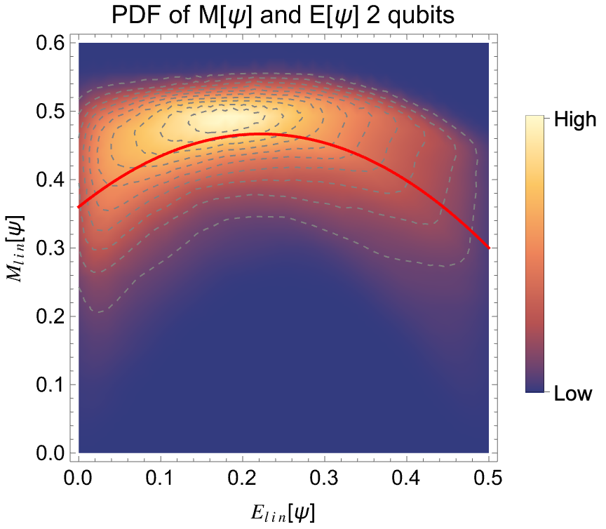
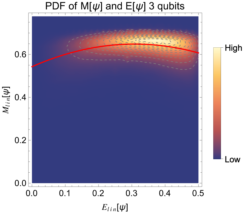
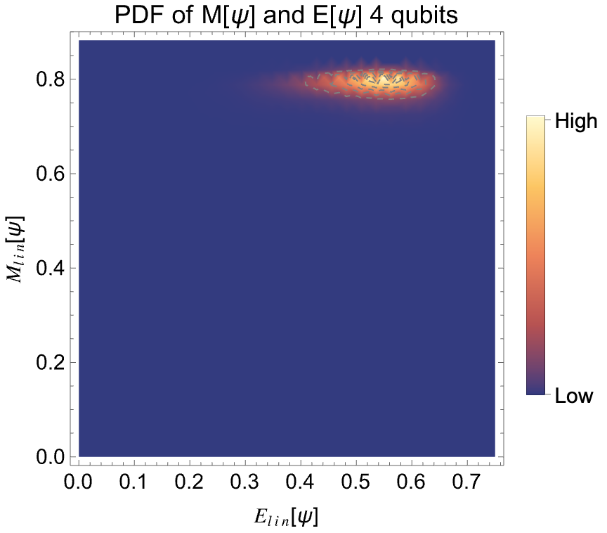
Numerical results for , , and are reported in Fig. 2(a), 2(b), 3.
In the large limit the above equation becomes
| (43) |
concluding that it approaches almost a constant value as grows. One can recover the Haar average result by integrating over all possible values of entanglement
| (44) |
6 Entanglement-Magic duality through the lens of anti-flatness
The result described in Proposition 2 can be considered as follows from a generic perspective. A striking result in [18] is that a global quantity, , is equal to a local spectral quantity for the reduced density operator. This spectral quantity is the average anti-flatness of the reduced density operator over the Clifford orbit. Define such anti-flatness as
| (45) |
with then the theorem in [18] states that
| (46) |
with being Clifford unitaries and being the average over the Clifford group. Notice that the Clifford orbit preserves magic but changes the Schmidt coefficients.
We wonder if a dual statement is also true. Namely, we ask whether the average over the Schmidt orbit, that preserves the Schmidt coefficients but changes the magic yields a similar result, that is the antiflatness of the states on the orbit.
In order to more properly see such a duality between these statements we rewrite Eq. (25) as
| (47) |
where , and
| (48) |
The above expression gives the mean value of magic upon having fixed the value of entanglement as a function of the anti-flatness and the entanglement itself apart from a term proportional to . As one notices, the average magic is not entirely determined by the state’s anti-flatness. The supposed duality between entanglement and magic through anti-flatness, is thus broken. A sign that such symmetry is not perfect can be seen in the fact the Clifford group allows one to reach states with maximum entanglement whereas the converse is not true: one cannot reach maximum magic states by means of factorized unitaries.
This collection of facts paints a picture in which the interplay between magic and entanglement is not symmetric, in the sense that magic needs entanglement to reach its maximal values, whereas entanglement does not need magic, due to the very relationship between the set of free operations of the two resources. The anti-flatness seems to capture some properties of both magic and entanglement, although imperfectly.
7 Conclusions and Outlook
This work establishes some technical results regarding the relationship between magic and entanglement in random states. We show that the two quantities are perfectly uncorrelated (in their linear versions) yet strongly dependent, which is a very non-trivial statistical result.
We then compute the average magic on the Schmidt orbit, namely the average magic once the Schmidt coefficients of a bipartite state have been fixed. The result is that, in first approximation, the average over the Schmidt orbit is given by the linear entanglement, in second approximation, by the anti-flatness of the reduced density operator, plus other terms that break the duality between Clifford orbits and Schmidt orbits. Finally, we show that these results show typicality in the Hilbert space.
In perspective, it would be important to deepen this analysis by finding exact results on the probability of magic conditioned to entanglement. These results will also constitute some useful tools for the study of the resource theory of non-local magic as well as the scrambling and spreading of magic in local quantum systems.
8 Acknowledgments
The authors would like to thank G. Ascione for clarifications about the concentration of measure for products of spheres. Additionally, the authors recognize the fruitful discussions on the matter with S. Cusumano and G. Scuotto. This research was funded by the Research Fund for the Italian Electrical System under the Contract Agreement "Accordo di Programma 2022–2024" between ENEA and Ministry of the Environment and Energetic Safety (MASE)- Project 2.1 "Cybersecurity of energy systems". AH acknowledges support from the PNRR MUR project PE0000023-NQSTI and the PNRR MUR project CN 00000013-ICSC and stimulating conversation with G. Zaránd.
References
- [1] R. Horodecki, P. Horodecki, M. Horodecki, and K. Horodecki, “Quantum entanglement,” Reviews of Modern Physics, vol. 81, pp. 865–942–865–942, June 2009.
- [2] D. Gottesman, “The Heisenberg Representation of Quantum Computers,” July 1998.
- [3] M. A. Nielsen and I. L. Chuang, Quantum Computation and Quantum Information: 10th Anniversary Edition. Cambridge University Press, 2010.
- [4] E. Chitambar and G. Gour, “Quantum resource theories,” Review of Modern Physics, vol. 91, pp. 025001–025001, Apr. 2019.
- [5] E. T. Campbell, “Catalysis and activation of magic states in fault-tolerant architectures,” Physical Review A, vol. 83, pp. 032317–032317, Mar. 2011.
- [6] S. Bravyi, G. Smith, and J. A. Smolin, “Trading Classical and Quantum Computational Resources,” Physical Review X, vol. 6, pp. 021043–021043, June 2016.
- [7] M. Beverland, E. Campbell, M. Howard, and V. Kliuchnikov, “Lower bounds on the non-Clifford resources for quantum computations,” Quantum Science and Technology, vol. 5, pp. 035009–035009, June 2020.
- [8] L. Leone, S. F. Oliviero, and A. Hamma, “Stabilizer Rényi Entropy,” Physical Review Letters, vol. 128, no. 5, p. 050402, 2022.
- [9] L. Leone, S. F. Oliviero, and A. Hamma, “Nonstabilizerness determining the hardness of direct fidelity estimation,” Physical Review A, vol. 107, no. 2, p. 022429, 2023.
- [10] K. Goto, T. Nosaka, and M. Nozaki, “Chaos by Magic,” Dec. 2021.
- [11] R. J. Garcia, K. Bu, and A. Jaffe, “Resource theory of quantum scrambling,” Proceedings of the National Academy of Sciences, vol. 120, no. 17, p. e2217031120, 2023.
- [12] D. Fattal, T. S. Cubitt, Y. Yamamoto, S. Bravyi, and I. L. Chuang, “Entanglement in the stabilizer formalism,” arXiv preprint quant-ph/0406168, 2004.
- [13] A. Hamma, R. Ionicioiu, and P. Zanardi, “Bipartite entanglement and entropic boundary law in lattice spin systems,” Physical Review A, vol. 71, pp. 022315–022315, Feb. 2005.
- [14] O. C. O. Dahlsten and M. B. Plenio, “Entanglement probability distribution of bi-partite randomised stabilizer states,” Quant. Inf. Comput., vol. 6, no. 6, pp. 527–538, 2006.
- [15] C. Chamon, A. Hamma, and E. R. Mucciolo, “Emergent Irreversibility and Entanglement Spectrum Statistics,” Physical Review Letters, vol. 112, pp. 240501–240501, June 2014.
- [16] L. Leone, S. F. E. Oliviero, Y. Zhou, and A. Hamma, “Quantum Chaos is Quantum,” Quantum, vol. 5, p. 453, May 2021.
- [17] S. Zhou, Z.-C. Yang, A. Hamma, and C. Chamon, “Single T gate in a Clifford circuit drives transition to universal entanglement spectrum statistics,” SciPost Phys., vol. 9, p. 087, 2020.
- [18] E. Tirrito, P. S. Tarabunga, G. Lami, T. Chanda, L. Leone, S. F. Oliviero, M. Dalmonte, M. Collura, and A. Hamma, “Quantifying nonstabilizerness through entanglement spectrum flatness,” Physical Review A, vol. 109, no. 4, p. L040401, 2024.
- [19] A. Gu, S. F. Oliviero, and L. Leone, “Magic-induced computational separation in entanglement theory,” arXiv preprint arXiv:2403.19610, 2024.
- [20] L. Leone and L. Bittel, “Stabilizer entropies are monotones for magic-state resource theory,” Phys. Rev. A, vol. 110, p. L040403, Oct 2024.
- [21] D. Szombathy, A. Valli, C. P. Moca, L. Farkas, and G. Zaránd, “Independent stabilizer Rényi entropy and entanglement fluctuations in random unitary circuits,” 1 2025.
- [22] S. Bravyi and A. Kitaev, “Universal quantum computation with ideal Clifford gates and noisy ancillas,” Physical Review A, vol. 71, pp. 022316–022316, Feb. 2005.
- [23] M. Howard and E. Campbell, “Application of a Resource Theory for Magic States to Fault-Tolerant Quantum Computing,” Physical Review Letters, vol. 118, pp. 090501–090501, Mar. 2017.
- [24] V. Veitch, S. A. H. Mousavian, D. Gottesman, and J. Emerson, “The Resource Theory of Stabilizer Quantum Computation,” New Journal of Physics, vol. 16, pp. 013009–013009, Jan. 2014.
- [25] L. Leone, S. F. E. Oliviero, and A. Hamma, “Stabilizer Rényi Entropy,” Physical Review Letters, vol. 128, pp. 050402–050402, Feb. 2022.
- [26] E. Lubkin, “Entropy of an n-system from its correlation with a k-reservoir,” Journal of Mathematical Physics, vol. 19, no. 5, pp. 1028–1031, 1978.
- [27] D. N. Page, “Average entropy of a subsystem,” Physical Review Letters, vol. 71, pp. 1291–1294–1291–1294, Aug. 1993.
- [28] S. Lloyd, Black Holes, Demons and the Loss of Coherence: How Complex Systems Get Information, and What They Do with It. PhD thesis, Rockefeller University, 1988.
- [29] A. J. Scott and C. M. Caves, “Entangling power of the quantum Baker’s map,” Journal of Physics A: Mathematical and General, vol. 36, no. 36, p. 9553, 2003.
- [30] P. Hayden, D. W. Leung, and A. Winter, “Aspects of Generic Entanglement,” Communications in Mathematical Physics, vol. 265, pp. 95–117–95–117, Mar. 2006.
- [31] H. Zhu, R. Kueng, M. Grassl, and D. Gross, “The Clifford group fails gracefully to be a unitary 4-design,” Sept. 2016.
- [32] I. Bengtsson and K. Zyczkowski, Geometry of Quantum States: An Introduction to Quantum Entanglement. Cambridge: Cambridge University Press, 2006.
- [33] S. Lloyd and H. Pagels, “Complexity as thermodynamic depth,” Annals of Physics, vol. 188, pp. 186–213, Nov. 1988.
- [34] K. Zyczkowski and H.-J. Sommers, “Induced measures in the space of mixed quantum states,” J. Phys. A: Math. Gen., vol. 34, p. 7111, Aug. 2001.
- [35] O. Giraud, “Distribution of bipartite entanglement for random pure states,” Journal of Physics A: Mathematical and Theoretical, vol. 40, no. 11, p. 2793, 2007.
- [36] O. Giraud, “Purity distribution for bipartite random pure states,” Journal of Physics A: Mathematical and Theoretical, vol. 40, no. 49, p. F1053, 2007.
- [37] G. Biswas, S.-H. Hu, J.-Y. Wu, D. Biswas, and A. Biswas, “Fidelity and entanglement of random bipartite pure states: insights and applications,” Phys. Scr., vol. 99, p. 075103, June 2024. Publisher: IOP Publishing.
- [38] C. Cao, G. Cheng, A. Hamma, L. Leone, W. Munizzi, and S. F. Oliviero, “Gravitational back-reaction is the holographic dual of magic,” arXiv preprint arXiv:2403.07056, 2024.
- [39] R. Bhatia and C. Davis, “A Better Bound on the Variance,” The American Mathematical Monthly, vol. 107, pp. 353–357–353–357, Apr. 2000.
- [40] V. Milman, “The heritage of P. Lévy in geometrical functional analysis,” Astérisque, vol. 157, no. 158, pp. 273–301, 1988.
- [41] M. Ledoux, The Concentration of Measure Phenomenon. American Mathematical Society, Feb. 2005.
- [42] L. Nachbin, The Haar Integral. R. E. Krieger Publishing Company, 1976.
- [43] D. A. Roberts and B. Yoshida, “Chaos and complexity by design,” Journal of High Energy Physics, vol. 2017, pp. 121–121, Apr. 2017.
- [44] A. A. Mele, “Introduction to Haar measure tools in Quantum Information: A beginner’s tutorial,” Quantum, vol. 8, p. 1340, 2024.
- [45] S. F. E. Oliviero, L. Leone, F. Caravelli, and A. Hamma, “Random Matrix Theory of the Isospectral twirling,” SciPost Physics, vol. 10, pp. 76–76, 2021.
Appendix A Haar integration over the flag manifold
If is a normal subgroup of a group one can define the quotient space which has also a group structure. If on there is a (unique) Haar measure , this induces a Haar measure on , , and on the quotient , . The measures satisfy the following relation
| (49) |
In fact the above equation can be seen as a way to define a Haar measure on the quotient (see e.g. [42]). We now use the above relation with and . The functions we are interested in, are and . Both of these functions are invariant under the action of . In fact is a function of the singular value decomposition (Schmidt decomposition) which is invariant under this symmetry while the entanglement is only a function of the Schmidt coefficients (and not of the unitaries and ). Hence, for our case we have
| (50) |
this means that we can replace Haar integration over the quotient with Haar integration over the original group , that is we obtain Eq. (19) of the main text.
Appendix B Permutations conjugacy classes
In this section a summary of the conjugacy classes of the symmetric groups of order 4, 6 and 8 is shown since they are heavily used in the computations of the variance of and for the covariance between and .
| Cycle type | Size of conjugacy class |
|---|---|
| – the identity element | 1 |
| 6 | |
| 3 | |
| 8 | |
| 6 |
| Cycle type | Size of conjugacy class |
|---|---|
| () – the identity element | 1 |
| 15 | |
| 40 | |
| 90 | |
| 45 | |
| 144 | |
| 120 | |
| 15 | |
| 90 | |
| 40 | |
| 120 |
| Representative element | Size of conjugacy class |
|---|---|
| 1 | |
| 28 | |
| 112 | |
| 420 | |
| 210 | |
| 1344 | |
| 1120 | |
| 3360 | |
| 2520 | |
| 420 | |
| 1120 | |
| 5760 | |
| 1680 | |
| 3360 | |
| 4032 | |
| 105 | |
| 1260 | |
| 1120 | |
| 3360 | |
| 2688 | |
| 1260 | |
| 5040 |
Appendix C On a peculiar pattern of traces and Pauli strings
In the subsequent calculations, a lot of terms of the form will be encountered: one can extract a rule to compute the sum over and .
Given two Pauli strings and , then
| (51) |
for , the number of qubits and .
One can start by writing
| (52) |
where and with that defines the Pauli matrices. Now define
| (53) |
then
| (54) |
A close formula form can be written for , namely all the combinations of Pauli matrices reads
| (55) |
and the trace of the -power
| (56) |
where and the fact that for . Finally one has
| (57) |
A simple check can be made for , namely
| (58) | ||||
| (59) | ||||
| (60) | ||||
| (61) |
with the swap over the two copies. Extending the strategy further by computing
| (62) |
| (63) |
for , the number of qubits and .
Appendix D Explicit calculations for the SE variance
Now we show the explicit calculations for the fluctuations of is carried out, i.e.
| (64) |
with . The fluctuations will be computed according to the Haar measure
| (65) |
using [8]. The main calculation revolves around
| (66) |
The authors in [43, 44] show that the Haar average of copies of a pure density operator is given by
| (67) |
where the sum runs over the elements of the symmetric group of order . Substituting this expression for in Eq. (66) and explicit expansion of yields the following:
| (68) |
In order to compute the traces in (68), the following property of permutation operators has been used [45]:
| (69) |
where is a permutation comprised of cycles , each of length respectively. However, the numbers of elements of in Eq. (68) renders a one-by-one manual evaluation unfeasible: the calculation will be approached by dividing the permutations in conjugacy classes/cycle types, using the data from Table 3. The passages are shown below:
cycles
| (70) |
cycles
| (71) |
cycles
| (72) |
cycles
| (73) |
cycles
| (74) |
cycles
| (75) |
cycles
| (76) |
cycles
| (77) |
cycles
| (78) |
cycles
| (79) |
cycles
| (80) |
cycles
| (81) |
cycles
| (82) |
cycles
| (83) |
| (84) |
cycles vspace-1pt
| (85) |
cycles
| (86) |
cycles
| (87) |
| (88) |
cycles
| (89) |
cycles
| (90) |
cycles
| (91) |
Summing every piece, one get
| (92) |
Hence the final result of the variance of reads
| (93) |
Appendix E Explicit calculation of the covariance between and
The object of this section is to show explicit calculations for . The object reads
| (94) |
The main calculation revolves around
| (95) |
Substituting the expression from Eq. (67) for the formula reads
| (96) |
where . Moreover, using the fact that , one can further write
| (97) |
Pulling the data from Table 2, one computes the sums over permutations according to conjugacy class: calculations follow below.
- Identity
| (98) |
- cycles
| (99) |
- cycles
| (100) |
- cycles
| (101) |
- cycles
| (102) |
- cycles
| (103) |
- cycles
| (104) |
- cycles
| (105) |
- cycles
| (106) |
- cycles
| (107) |
- cycles
| (108) |
Summing all those pieces together, one gets
| (109) |
and finally
| (110) |
Appendix F Explicit calculation of the average linear SE over the orbit of factorized unitaries
The objective of this section is to show the calculations needed to compute the following average:
| (111) |
with , with without loss of generality. Here and are to be thought of as generic orthonormal vectors on the respective Hilbert spaces. After a proper permutation, i.e. , one can write the expression using the Weingarten calculus as [44]
| (112) |
with being the Weingarten function, defined as the pseudo inverse of the Gram matrix . The computation will be carried out by noting the result of the traces is symmetric between the two partitions and this means one has to compute the following terms. The order of the permutations of as well as the results of and are summarized in Table 4 below.
| Id | ||
After carrying out the contraction of the product of Schmidt coefficients with the proper Kronecker deltas, summing up the terms for all permutations and rearranging the terms one finally gets
| (113) |
with defined as per Eq. (26) and
| (114) |
Proper rearrangement of the terms and collecting yields the expression seen in Eq. (25) which has the explicit dependence on entanglement.