Principal Components for Neural Network Initialization
Abstract
Principal Component Analysis (PCA) is a commonly used tool for dimension reduction and denoising. Therefore, it is also widely used on the data prior to training a neural network. However, this approach can complicate the explanation of explainable AI (XAI) methods for the decision of the model. In this work, we analyze the potential issues with this approach and propose Principal Components-based Initialization (PCsInit), a strategy to incorporate PCA into the first layer of a neural network via initialization of the first layer in the network with the principal components, and its two variants PCsInit-Act and PCsInit-Sub. Explanations using these strategies are as direct and straightforward as for neural networks and are simpler than using PCA prior to training a neural network on the principal components. Moreover, as will be illustrated in the experiments, such training strategies can also allow further improvement of training via backpropagation.
Index Terms:
deep learning, neural networks, classificationI Introduction
Principal Component Analysis (PCA) is a widely used dimensionality reduction technique that transforms high-dimensional data into a lower-dimensional space while preserving as much variance as possible. By identifying the principal components, which are the orthogonal directions that capture the most variance in the data, PCA helps to eliminate redundancy, improve computational efficiency, and mitigate the effects of noise. It achieves this through eigenvalue decomposition of the covariance matrix or singular value decomposition (SVD) of the data matrix. PCA is extensively applied in fields such as machine learning, image processing, and bioinformatics to uncover patterns, visualize high-dimensional data, and enhance model performance by reducing overfitting.
In the context of neural network training, PCA offers significant advantages by decorrelating the input features, which in turn leads to a better-conditioned Hessian matrix. This is crucial because a poorly conditioned Hessian, often caused by correlated features, can result in slow convergence during gradient-based optimization, leading to inefficiencies in training [1]. By transforming the input data into a set of orthogonal principal components, PCA ensures that gradient updates during backpropagation are more stable and effective, reducing the likelihood of oscillations or excessive adjustments along certain directions [2]. As a result, the optimization process becomes more efficient, with faster convergence toward the optimal solution. This makes PCA a valuable preprocessing technique for reducing the computational cost and enhancing the performance of neural networks, particularly in high-dimensional settings where the curse of dimensionality and correlated features are common [3]. Consequently, incorporating PCA in the training pipeline can lead to significant improvements in both speed and accuracy for models trained on complex, high-dimensional datasets [4]. Therefore, it is common to train neural networks on the principal components (PCA-NN).
However, this approach also has some limitations. First, the dimensionality reduction performed by PCA leads to a loss of information, meaning the back-projected gradients in the original input space may not fully capture the network’s behavior. Second, the principal components are linear combinations of original features, which may make the resulting features harder to interpret compared to the original data. So, while one can use the PCA loading matrix to transform back to the original features requires using the PCA loading matrix, which defines the contribution of each original feature to each principal component, applying PCA prior to training a neural network as in PCA-NN complicates the explanation process due to the further transformation step in PCA. Therefore, we introduce Principal Components based Initialization (PCsInit), a novel initialization technique for the first layer of a neural network based on the principal components. In addition, we also introduce PCsInit-Act, which applies an activation layer after the principal components to increase the neural network ability of nonlinear patterns. Moreover, we also introduce PCsInit-Sub, another variant of PCsInit that compute the principal components based on the subset of the input to increase the computational efficiency for large datasets. Note that these approaches are different from Neural PCA (Principal Component Analysis), which refers to using neural networks to approximate Principal Component Analysis (PCA), a technique used for dimensionality reduction and feature extraction in machine learning.
In summary, our main contributions are as follows:
-
•
We introduce PCsInit, a novel method for incorporating PCA into neural networks through weight initialization rather than preprocessing, which simplifies the explainability pipeline while maintaining the benefits of PCA.
-
•
We propose two practical variants:
-
–
PCsInit-Act: Enhances nonlinear pattern recognition by adding activation functions after PCA-initialized layers
-
–
PCsInit-Sub: Enables efficient scaling to large datasets by computing principal components on data subsets
-
–
-
•
We provide a theoretical analysis showing how PCsInit improves optimization by conditioning the Hessian matrix, leading to faster convergence compared to standard initialization methods.
-
•
Through extensive experiments on multiple datasets, we demonstrate that PCsInit and its variants achieve comparable or better performance than traditional PCA preprocessing while offering simpler explainability
II Motivation: Explainability when PCA is applied before a neural network
When PCA is applied before a neural network (PCA-NN), perturbation-based XAI methods, such as LIME [5], Occlusion [6], and Feature Permutation [7], are heavily impacted because they rely on modifying input features and observing their effect on predictions. This is because perturbing the input features instead of the principal components directly affects the SVD of the input or the covariance matrix of the input and principal components are linear combinations of multiple features. On the other hand, if perturbations are applied to principal components, the results are meaningful only in the transformed PCA space. Mapping the effects back to the original features requires using the PCA loading matrix, which defines the contribution of each original feature to each principal component. By redistributing the changes in principal components proportionally to their feature weights in the loading matrix, approximate feature-level insights can be obtained. However, this process introduces inaccuracies because the dimensionality reduction step in PCA discards some variance, and the transformation is not fully invertible. Overall, perturbation-based XAI methods are inherently less interpretable in PCA-NN pipelines because the transformations obscure the direct relationship between input features and predictions.
Next, let us consider gradient-based XAI methods. In a PCA-NN pipeline, the original input data is transformed into a lower-dimensional representation , where is the PCA projection matrix and is the mean of the input data, before being passed to the neural network. Gradient-based visualization methods such as saliency maps [8] and Grad-CAM [9], which rely on backpropagating gradients from the network’s output to its input, can still be applied in this setup by mapping the gradients from the PCA-transformed space back to the original input space . This mapping can be achieved using the chain rule, where , and for PCA, the Jacobian . Consequently, gradients computed in the PCA space can be back-projected into the original input space to enable visualization. However, PCA may remove or distort fine-grained input features that are crucial for effective gradient-based visualization, potentially reducing the interpretability and quality of methods like saliency maps or SmoothGrad.
Next, while feature attribution methods like SHAP [10] and LIME [5] can still explain predictions in the PCA-transformed space, mapping these explanations back to the original feature space for explanation of the input requires leveraging the PCA loading matrix and comes with the limitation of approximation. To be more detailed, SHAP explains predictions by calculating feature contributions based on Shapley values. In a PCA-NN setup, SHAP can be applied directly to the PCA-transformed features . To attribute importance to the original input features , the contributions to must be back-projected to using the PCA matrix . However, may not be an invertible matrix. Therefore, the explanation is not complete, but rather an approximation. A similar thing happens to LIME. In summary, these methods can attribute importance in PCA-NN systems, but additional steps are required to map contributions from the reduced-dimensional PCA space back to the original input space, and the quality of these attributions depends on how much information is preserved by PCA.
On the other hand, if we can put PCA inside the neural network via initialization based on the similarity between the multiplication in PCA and the multiplication between neural network input and weight matrix, the explanation using XAI methods will be the same as for a regular neural network without applying PCA.
III Methodologies
In this section, we will introduce motivation and the formal training process of Principal Components Analysis Initialization (PCsInit), its two variations (PCsInit-Act, PCsInit-Sub), and relevant theoretical properties.
III-A Principal Components-based Initialization (PCsInit) - Basic Ideas.
This section details our proposed PCsInit framework. While PCA preprocessing requires maintaining and applying the transformation matrix during inference, PCsInit incorporates this information directly into the network weights, reducing operational complexity. Additionally, PCsInit allows the network to adaptively refine these initialized weights during training, potentially capturing more nuanced feature relationships that static PCA transformation might miss. Most importantly, PCsInit simplifies the explainability pipeline by eliminating the need to back-project through a separate PCA transformation step.
The basic idea of our proposed PCsInit approach using the PCA and the neural network can be described as follows. First, let , where , be an input data matrix of observations and features. Assume that the features are centered and scaled. Then, recall that the solution of PCA can be obtained using the singular value decomposition of :
| (1) |
where is an orthogonal matrix, is a orthogonal matrix, and is a diagonal matrix with diagonal elements . If eigenvalues are used, the projection matrix is , which consists of the first columns of . Then, the dimension-reduced version of is . This multiplication has some similarity with the multiplication between the input and the weight matrix of the first layer in a layer of a neural network. This motivates us to bring the PCA inside the neural network by simply initializing the first layer of a neural network with the principal components of the input and using no activation function for the first layer. The width of the first layer is chosen so that n_components is retained or so that percentage of the variance explained is retained. We call this strategy Principal Components-based intialization (PCsInit).
III-B Principal Components Analysis Initialization (PCsInit)
Formally, the training process of PCsInit is described in Algorithm 1. In the first step, PCA is applied to the entire input dataset to extract the top principal components, which are stored in the projection matrix . These principal components represent the directions of maximum variance in the data, allowing for an efficient lower-dimensional representation while preserving critical information.
In the second step, the matrix is used as the weight matrix for the first layer of a neural network . This initialization ensures that the first layer performs a transformation aligned with the most informative features of the input data, providing a strong inductive bias that can facilitate learning.
At the third step, to stabilize training and allow the deeper layers to adapt to the PCA-based initialization, the first layer is frozen, meaning its weights remain unchanged, while the remaining layers of the network are trained for epochs. This prevents drastic weight updates in the first layer, ensuring that the extracted principal components provide a meaningful starting point for training.
At the fourth step, after the deeper layers have sufficiently adapted, the first layer is unfrozen, allowing the entire neural network to be trained jointly for an additional epochs. This fine-tuning step enables all layers, including the first one, to update their parameters in a coordinated manner, optimizing the overall network performance and leading to better feature extraction and representation learning.
The reason for the initial frozen phase and then fine-tuning is that it allows the latter layers to adapt to the PCA-based feature space, establishing stable higher-level representations. Once these layers have learned effective feature combinations, unfreezing the first layer enables fine-tuning of the initial PCA-based weights while maintaining the learned feature hierarchy. This two-phase approach prevents early disruption of the meaningful PCA structure while allowing eventual optimization of all parameters.
PCsInit versus PCA prior to neural network. The goal of is to find the principal directions (eigenvectors of the covariance matrix) that capture the most variance in the data, while for neural networks, the weight matrix is learned through backpropagation to minimize a task-specific loss function. In addition, (the principal component directions) are computed directly from the data (using eigendecomposition or SVD) and are fixed once determined. Meanwhile, PCsInit for neural networks allows it to be adjusted iteratively during training for possible room for improvement.
Despite the differences, note that for the PCsInit approach, if the weights of the first layer are frozen throughout the training process then it is equivalent to applying PCA to the input data and then training a model on the principal components. Even in this case, using PCA in the PCsInit manner with the first layer frozen during training makes it easier to explain the model. Specifically, a neural network built upon principal components makes decisions based on a transformed feature space where the most significant variations in the data are captured. Since PCA reduces dimensionality by keeping only the most informative features, the network learns patterns in terms of these principal components rather than the original raw features. The decision can be explained by analyzing which principal components contributed most to the output, mapping them back to the original features, and using techniques like SHAP or sensitivity analysis. Meanwhile, PCsInit allows using SHAP and other XAI techniques directly on the input. Therefore, PCsInit offers a more straightforward explanation than explaining the decision of a neural network trained on principal components.
However, sometimes computing the principal components based on the whole input matrix can induce computational cost. Meanwhile, if the first layer is not completely frozen throughout training, it will be fine-tuned later. Therefore, it may be more computationally efficient to compute the principal components based on a subset of the input matrix instead. This is the motivation for Algorithm 2, which is a slight variation of Algorithm 1, where the principal components are computed based on a subset of the input matrix to reduce the computational expense associated with finding the principal components.
While PCsInit has the first layer similar to using PCA, the activation function is not applied after the first layer. Meanwhile, it is well known that activation functions are important in neural networks because they introduce non-linearity, allowing the model to learn complex patterns and relationships in data. In addition, they can also enable efficient gradient propagation during training. This motivates us to introduce another variation of PCsInit, namely PCsInit with Activation function (PCsInit-Act), which is described in Algorithm 3. It modifies PCsInit by applying an activation function after the first layer.
In summary, PCsInit-Act introduces an activation function during the initialization process, adding an additional layer of non-linearity. This enhancement improves the model’s ability to capture complex patterns within the data. On the other hand, PCsInit-Sub focuses on computational efficiency by utilizing a subset of the input data instead of the entire dataset during initialization. As will be illustrated in the experiment section, this approach provides a lightweight yet effective alternative for handling large datasets, maintaining competitive accuracy and stability while reducing computational costs. Together, these variations improve the flexibility of the PCsInit methodology, offering improved interpretability and adaptability to diverse datasets and computational constraints.
III-C Theoretical analysis
PCA transforms the data into uncorrelated features. Therefore, the Hessian matrix (second derivative of the loss) becomes more well-conditioned after PCA, making optimization more stable.
Theorem 1
Consider training a single-layer neural network for a linear regression problem, where we have the input matrix in , the label in , and we are using the weight matrix in . Then, PCA removes small eigenvalues of the Hessian matrix of the MSE loss function, leading to faster convergence.
Proof 1
It is known that the steepest descent method for nonlinear optimization is highly sensitive to scaling and the problem’s condition number and that convergence can be significantly slow when the condition number of the Hessian matrix is large [11].
For a linear regression problem with single-layer neural network, input matrix , the label , and the weight matrix , the Mean Squared Error (MSE) loss function is
Therefore, the gradient of the loss function with respect to is:
and the second derivative (Hessian) is
Thus, the Hessian depends on the structure of . Its eigenvalues determine how efficiently gradient descent converges. The condition number of the Hessian matrix is:
where and are the largest and smallest eigenvalues of .
When input features are highly correlated, some eigenvalues of become very small, making large and slowing optimization.
PCA transforms the input into uncorrelated principal components using an orthonormal transformation matrix :
Since is an orthonormal matrix (i.e., ), the covariance of is:
By construction, PCA diagonalizes , meaning the Hessian in the transformed space becomes:
where is a diagonal matrix containing the eigenvalues of .
Since PCA removes the smallest eigenvalues (low-variance directions), the condition number of is lower, leading to faster convergence.
IV Experiments
In this section, we will illustrate the performance of PCsInit and its variations compared to training neural network based on principal components (PCA-NN), and the performance of neural network without PCA (NN).
IV-A Experiment Settings
To illustrate the effectiveness of the proposed initialization strategies, we conduct various experiments on various datasets. The descriptions of the datasets used are as in Table I.
For each experiment, we choose the number of principal components so that a minimum of 95% of variance is retained, as commonly used in various research articles [12, 13, 14, 15]. The width of the network used for each dataset has a width equal to the number of principal components retained. All models are trained with a total of 200 epochs using Cross Entropy Loss and Adam optimizer with a learning rate of . The ReLU activation function is applied to all layers except the last layer. The number of layers used for all datasets is 5.
In PCsInit and its variations, the first layer is initialized with the principal components, and then it is frozen for the first 30 epochs. After that, we unfreeze this first layer and train the whole model for 170 more epochs. To facilitate a fair comparison, for all strategies, all layers are initialized with the same weights, except for the first layer, since PCsInit and its variants are initialized based on principal components, while PC-NN and NN are not. We compared each dataset with three different initialized techniques: He initialization, Xavier initialization, and Orthogonal initialization, and report the performance.
The experiments run on a CPU of AMD Ryzen 3 3100 4-Core Processor, installed RAM 16.0 GB. The codes for the experiments is available at github.com/pthnhan/pcsinit.
| Dataset | # Classes | # Features | # Samples |
|---|---|---|---|
| Heart | |||
| Ionosphere | |||
| Micromass | |||
| Parkinson |
The five datasets we evaluated are all of which involve binary classification and are categorized into two primary groups based on the number of features. The first group includes datasets with a smaller number of features such as Heart and Ionosphere. The second group consists of datasets with a larger number of features: MicroMass and Parkinson.
IV-B Results and Analysis
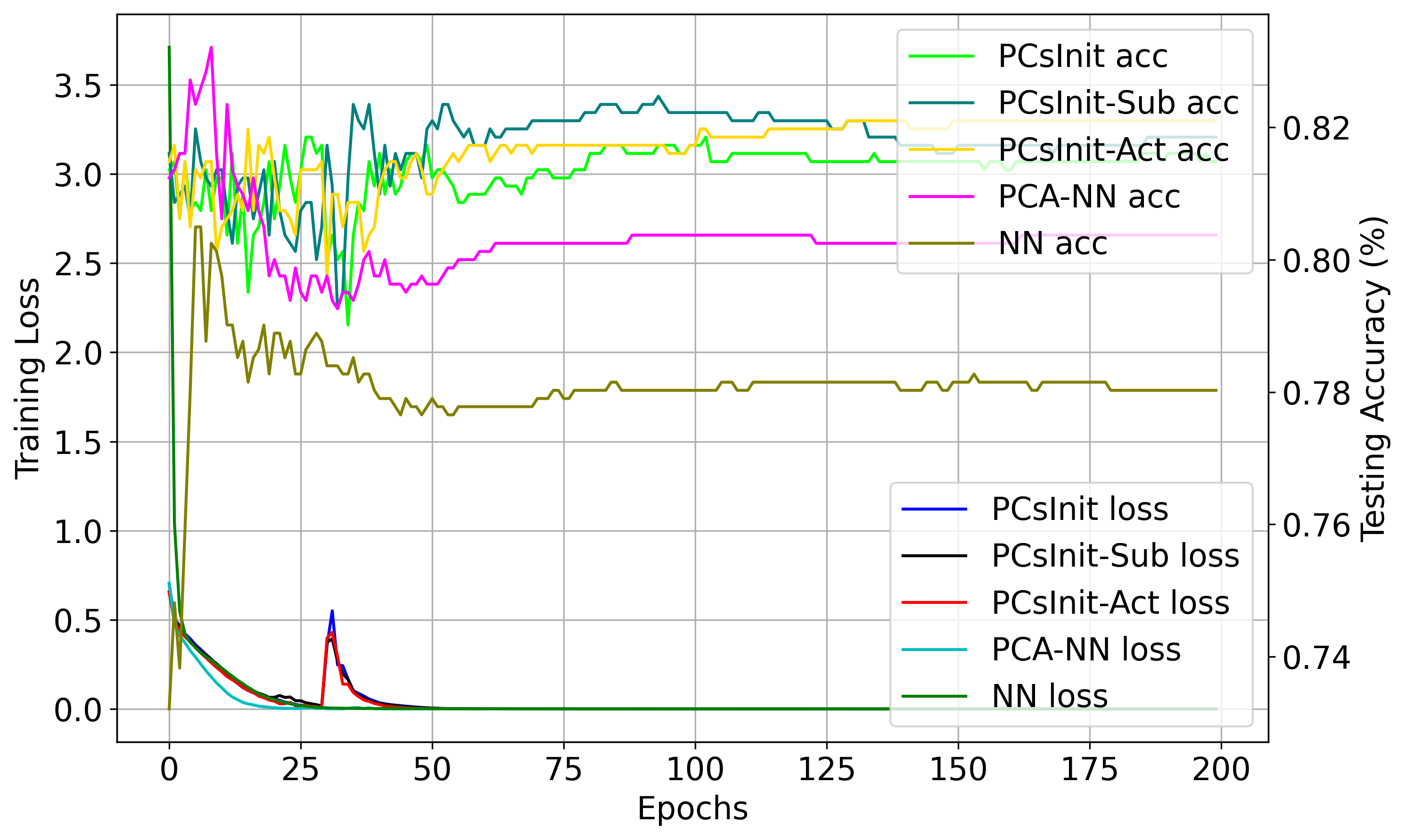
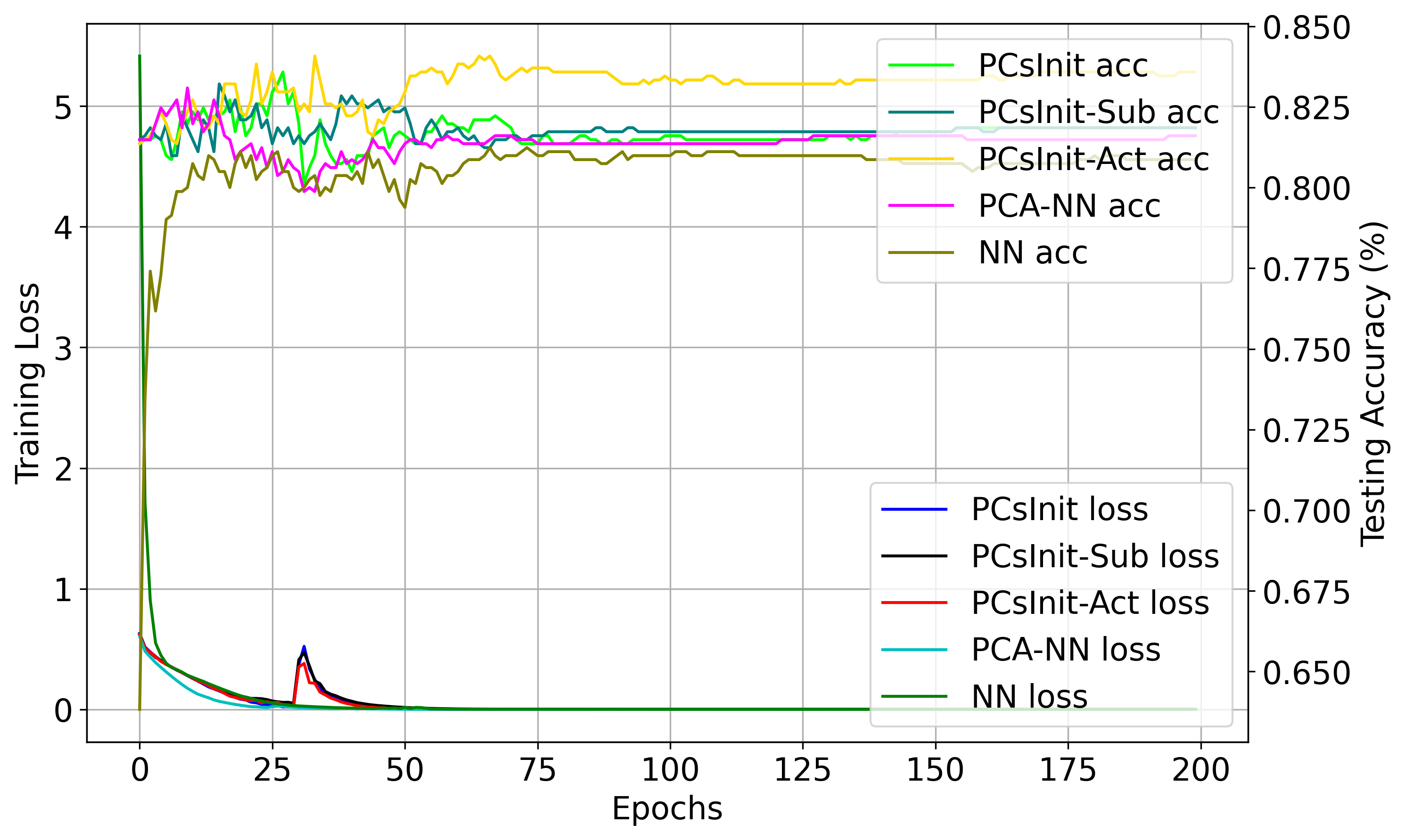
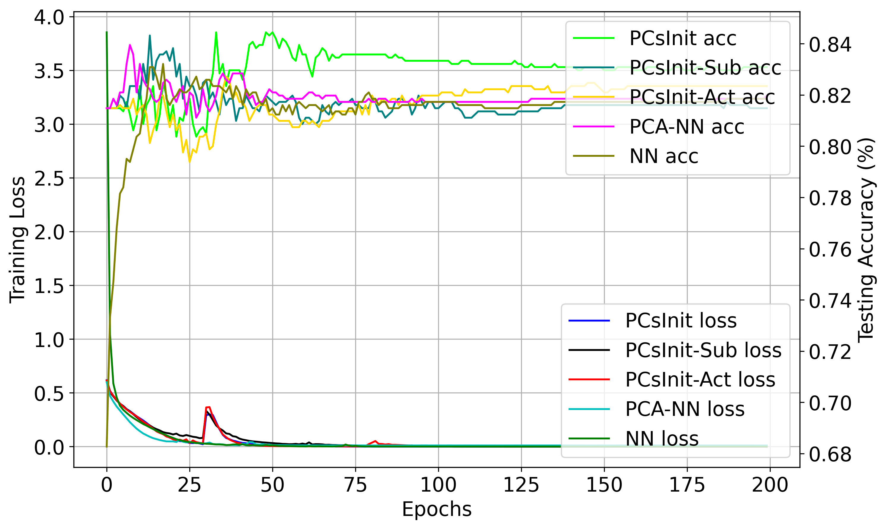
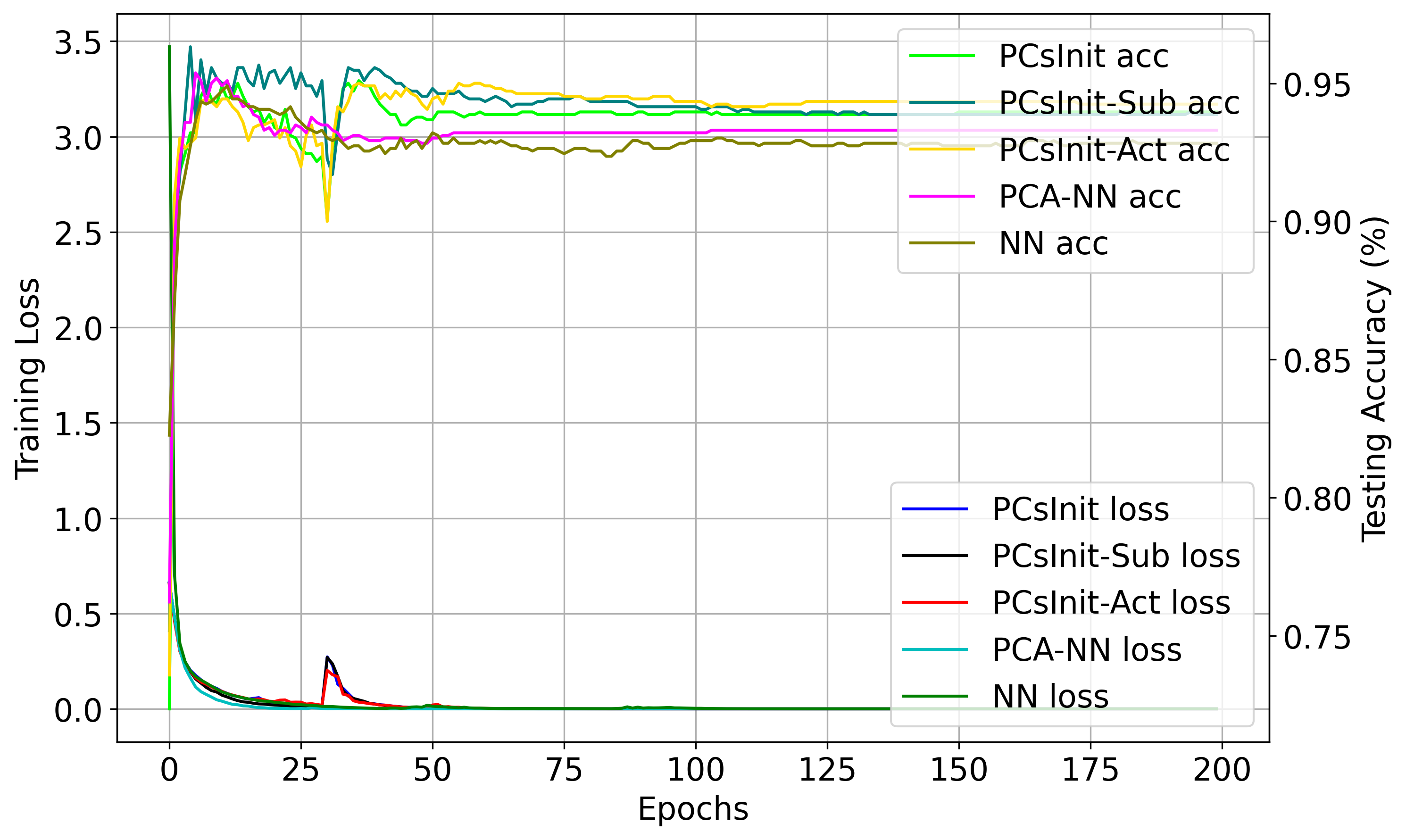
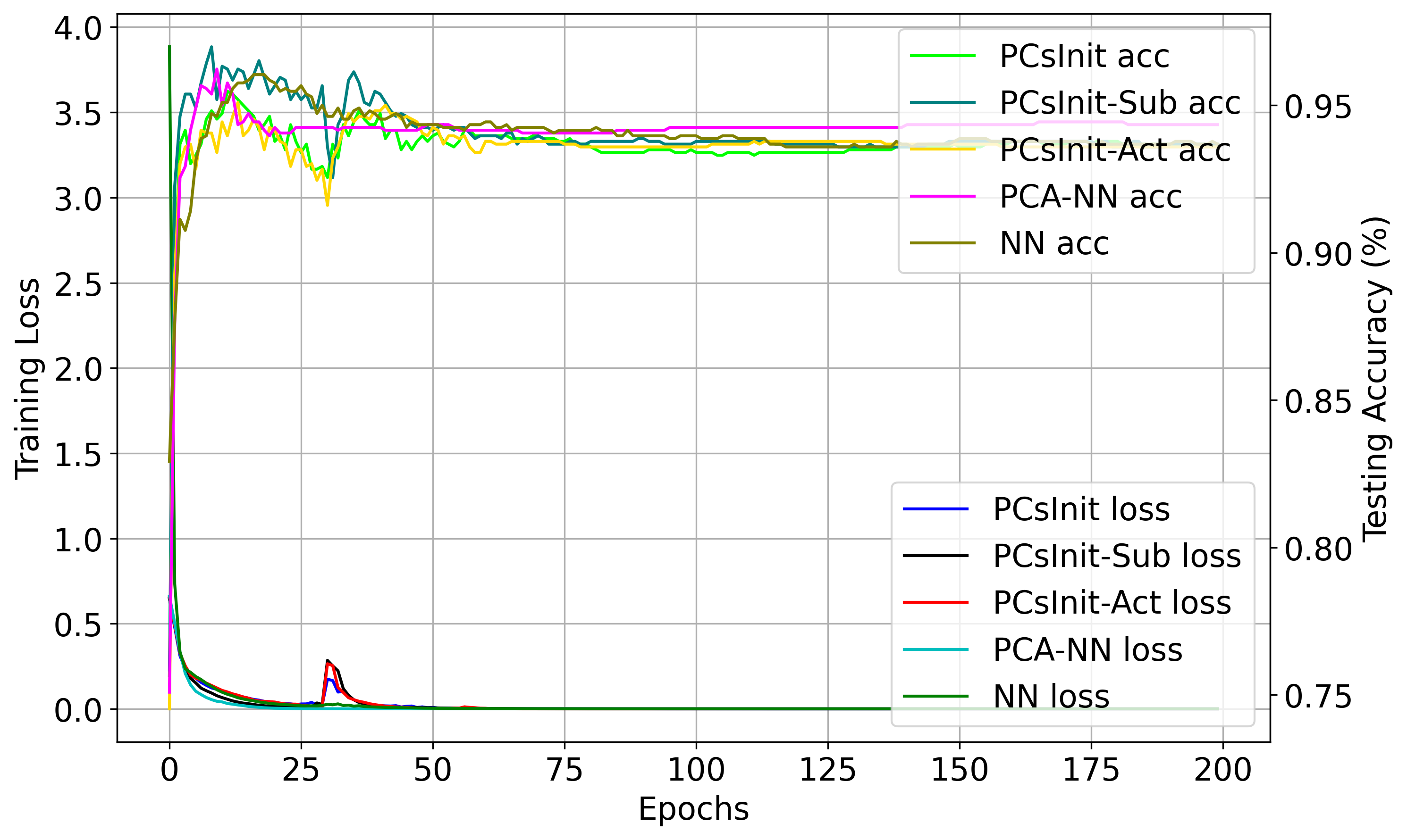
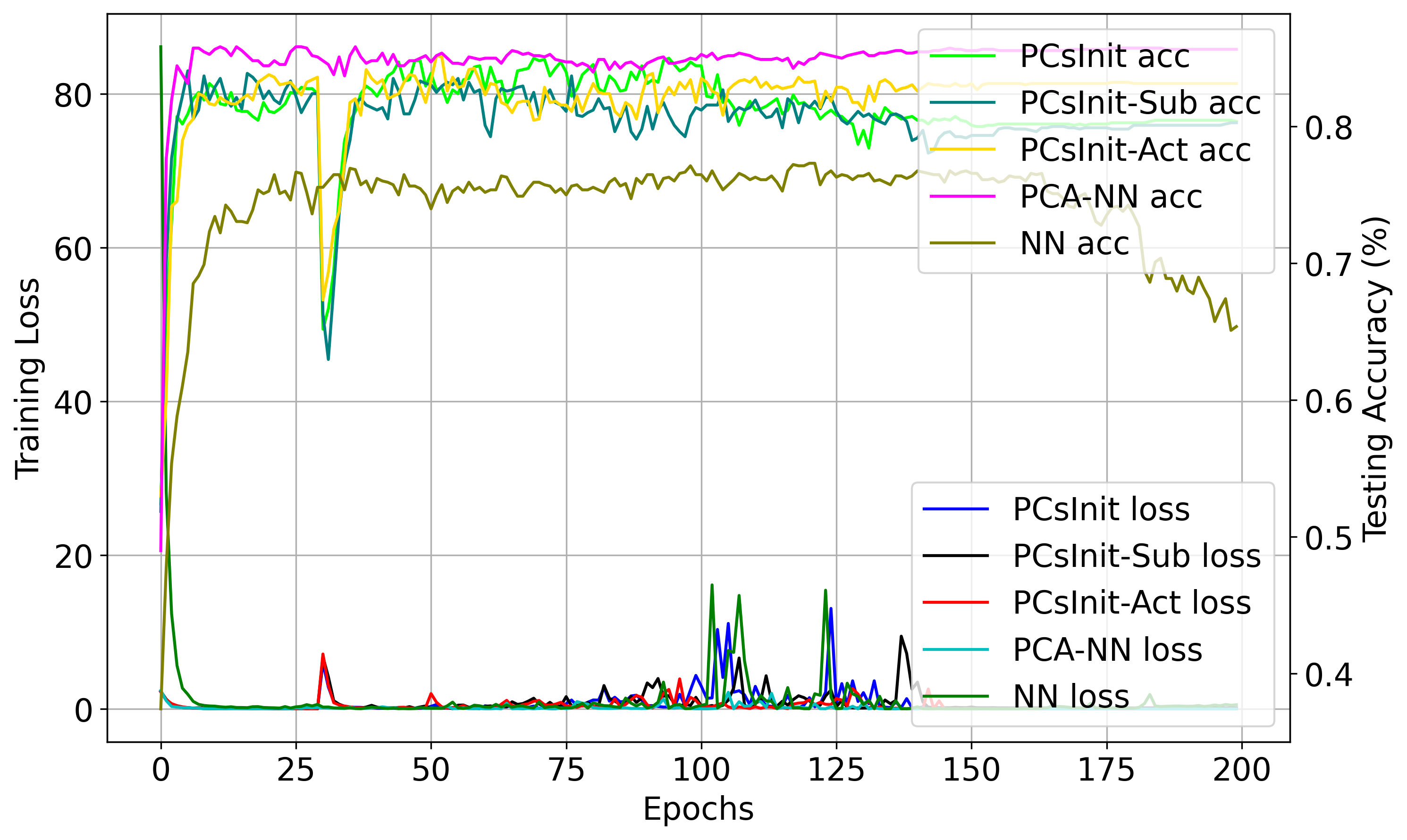
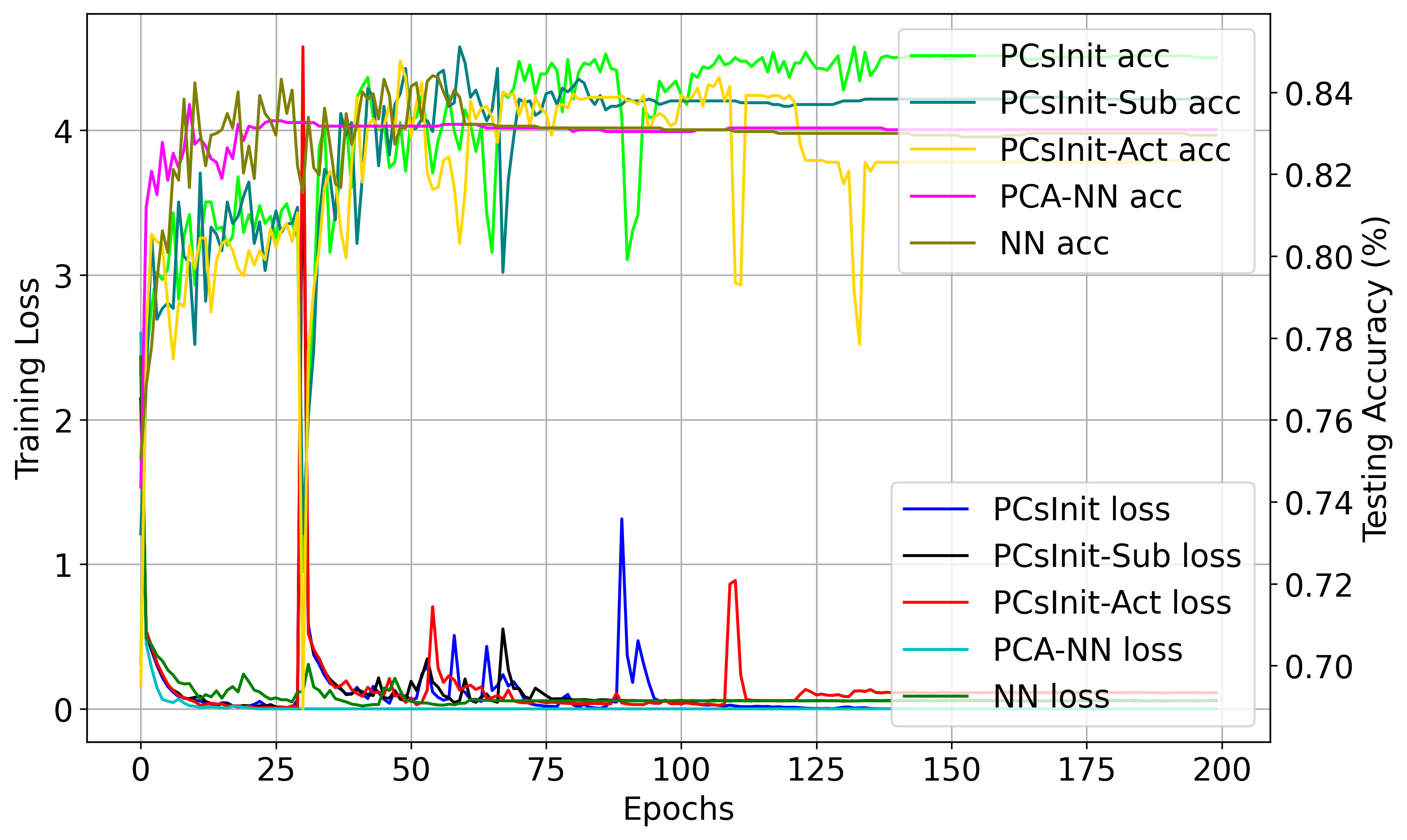
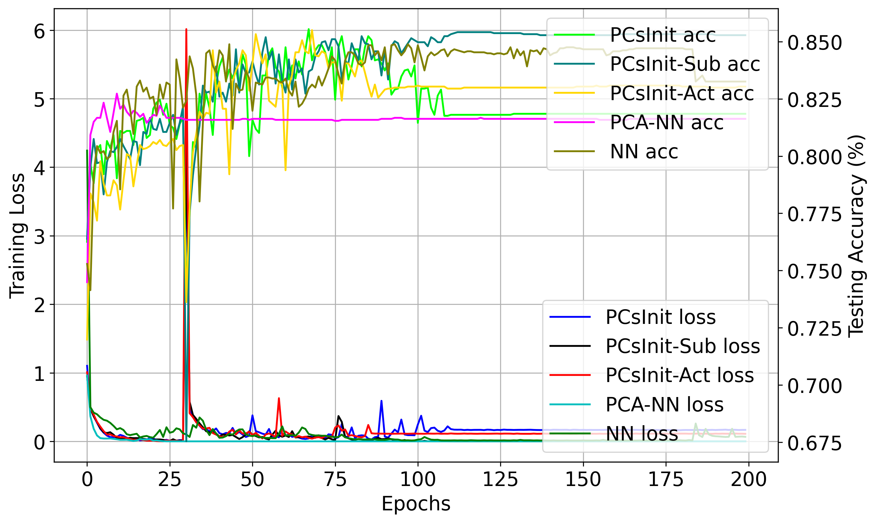
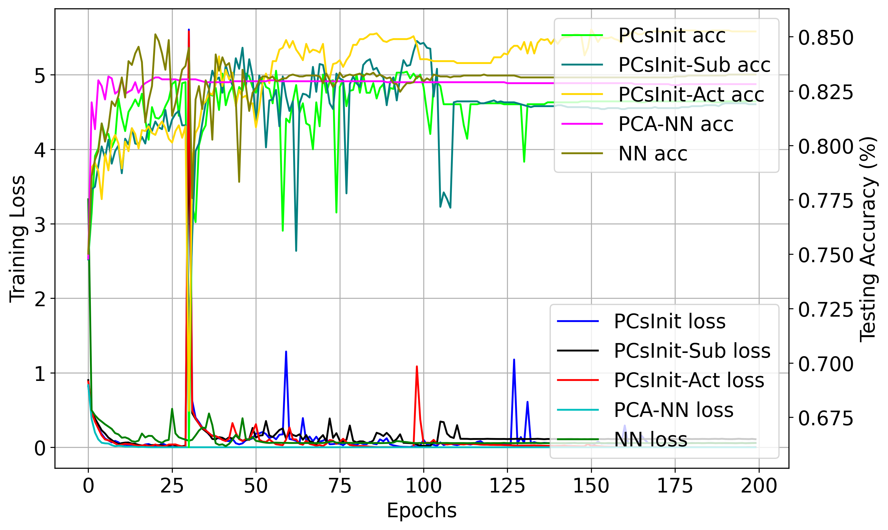
Our experiments cover a diverse set of datasets, ranging from datasets with few features to those where the number of features exceeds the number of samples (Micromass dataset). The experiments on these datasets illustrate the outperformance results of PCsInit, PCsInit-Act, PCsInit-sub, and PCA-NN compared to NN. Moreover, PCsInit and its variations also show excellent results in various data sets under three initialization techniques with better results compared to PCA-NN in both testing accuracy and convergence speed.
The experimental results demonstrate that PCsInit variations and PCA-NN outperform the standard NN initialization across most datasets and initialization techniques. In many cases, such as the Heart dataset, PCsInit consistently outperforms PCA-NN across all initialization techniques (figures 3, 3, 3), highlighting its adaptability and efficiency in optimizing the network’s performance.
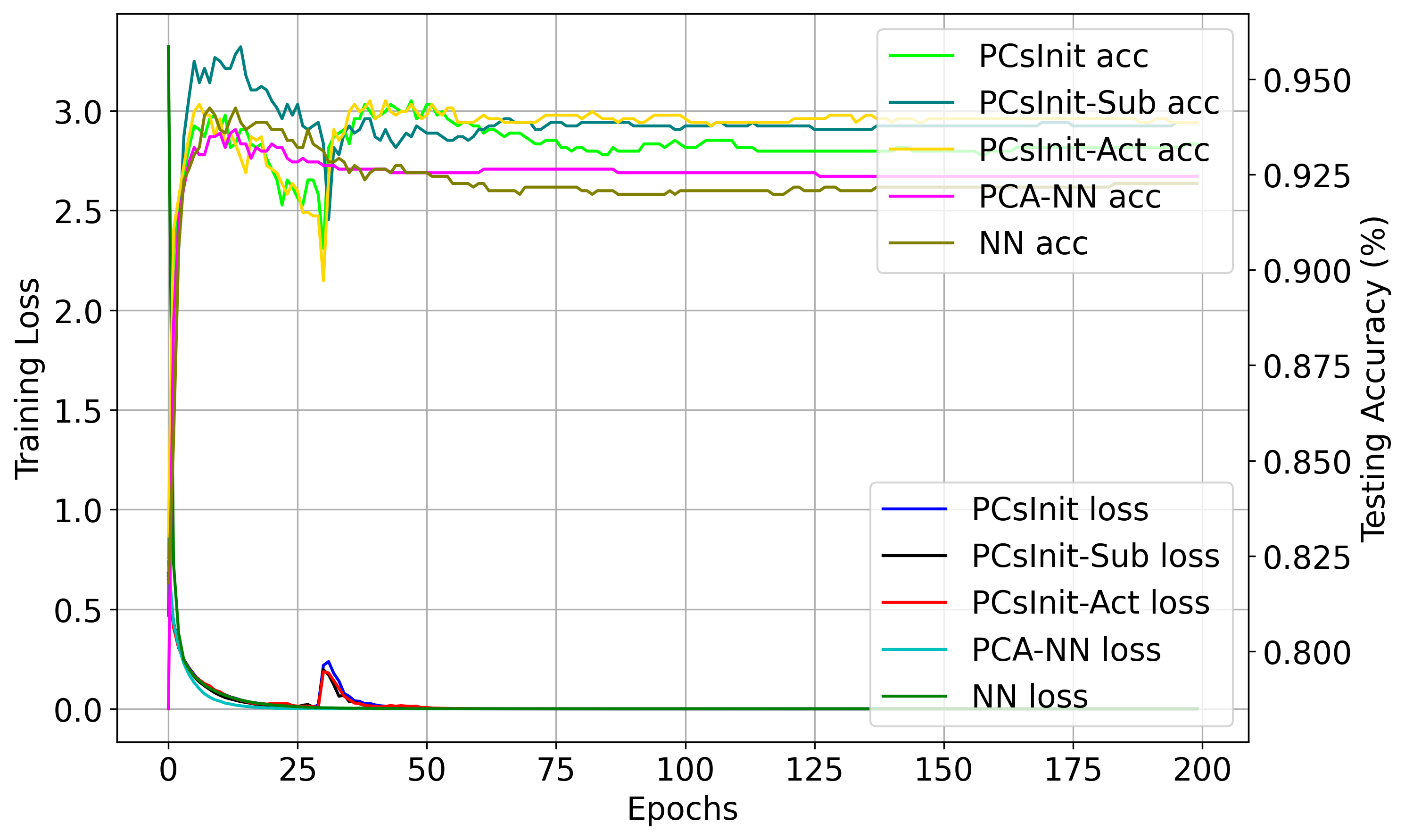
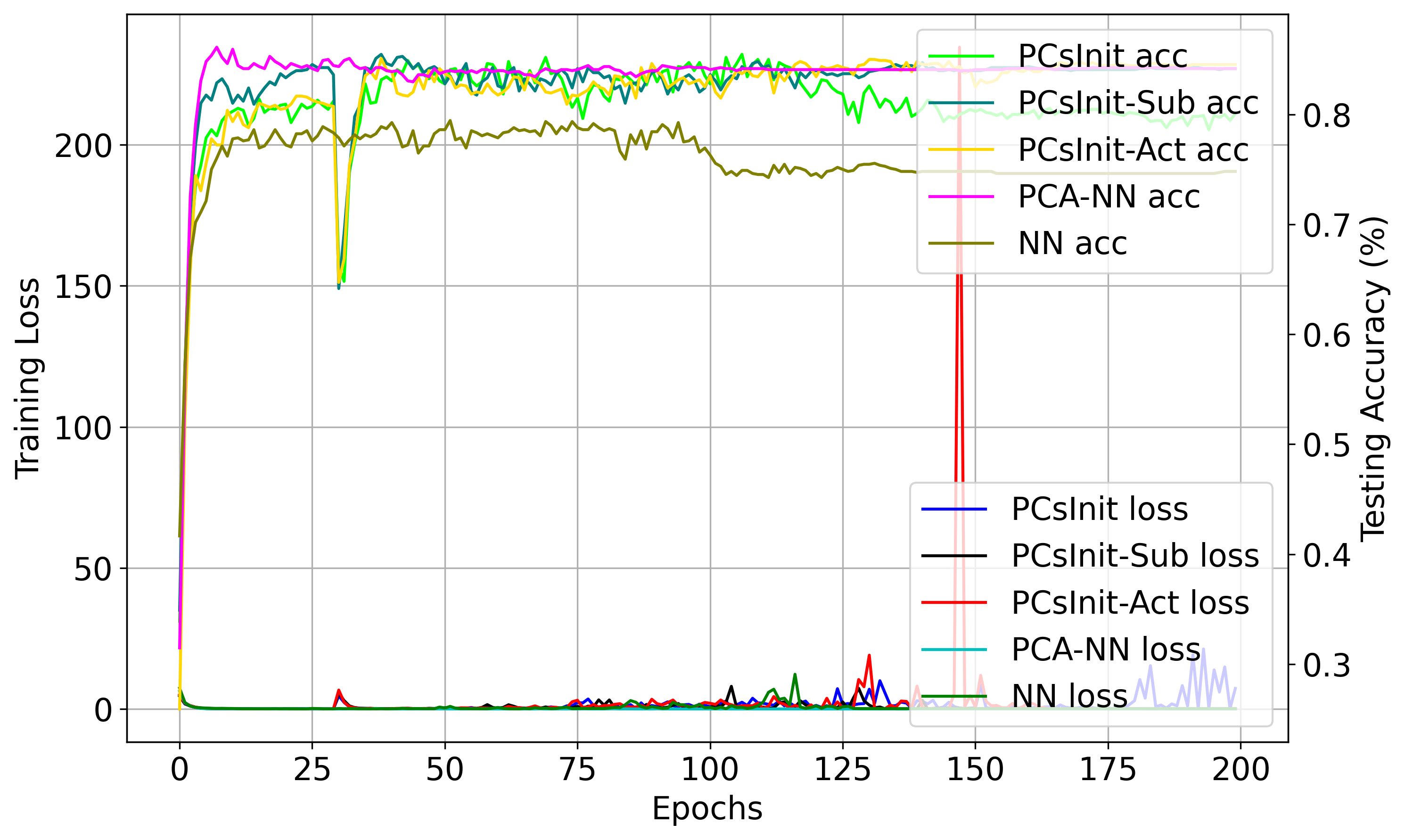
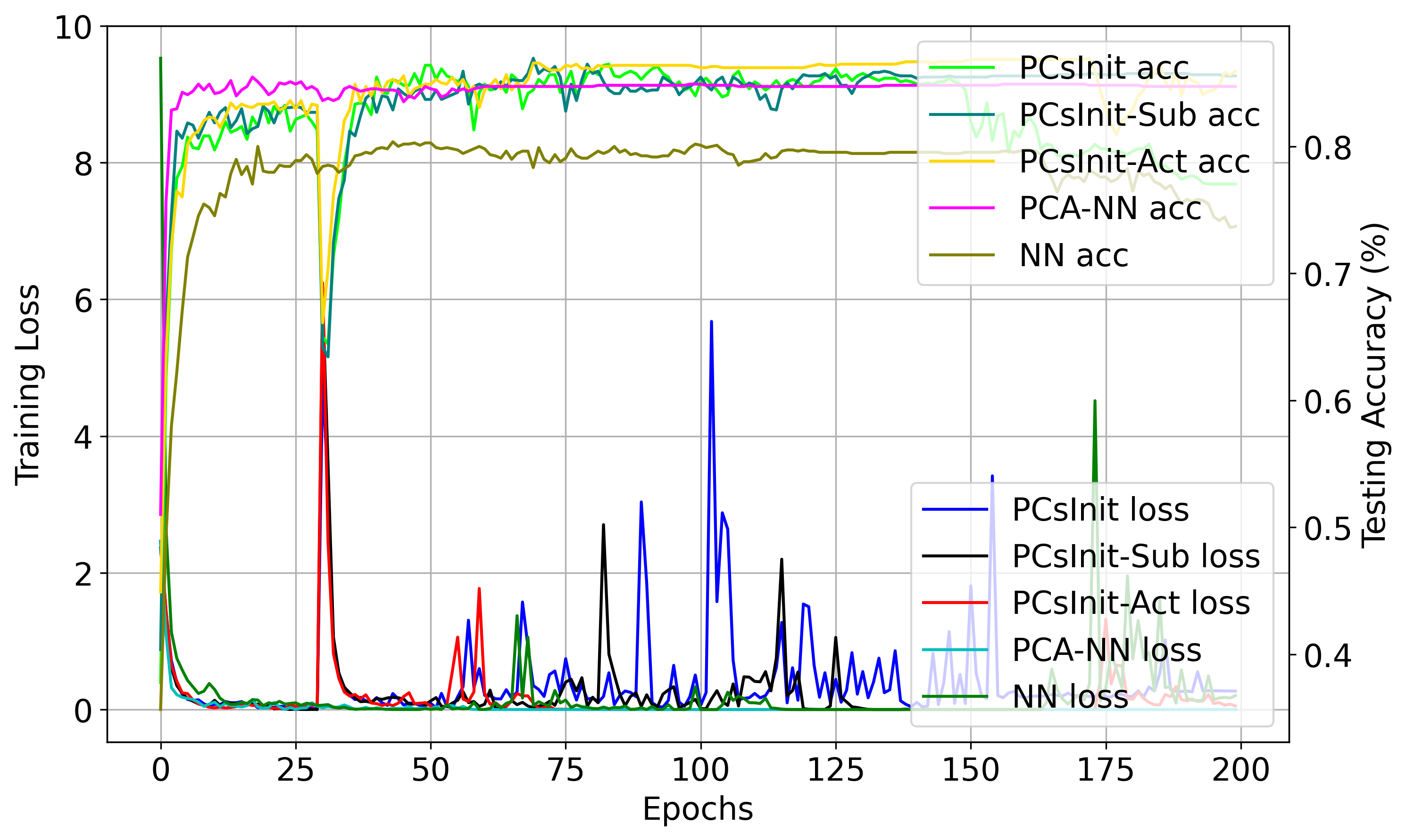
In some cases, PCsInit shows performance comparable to PCA-NN, particularly evident in the ionosphere dataset, where both methods achieve similar levels of accuracy and training loss stability. On the other hand, PCA-NN shows its strength on the micromass dataset, achieving higher accuracy compared to PCsInit. Notably, PCsInit-Sub on this dataset exhibits competitive performance with PCA-NN, demonstrating that it can achieve similar results while reducing computational costs. These findings underscore that while both PCsInit and PCA-NN provide substantial improvements over NN, the variations of PCsInit, such as PCsInit-Sub and PCsInit-Act, offer additional flexibility and adaptability, enabling robust performance across a broader range of scenarios.
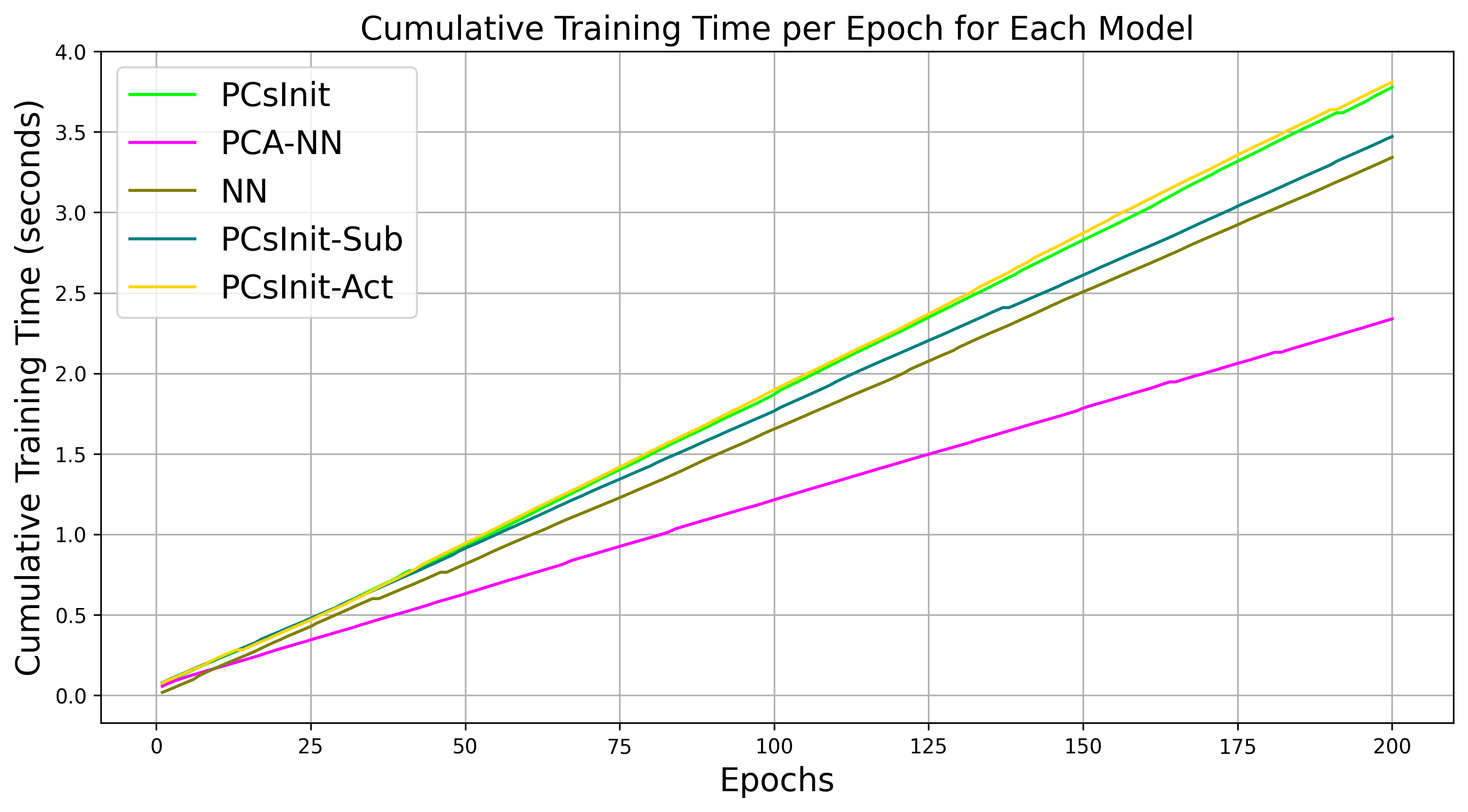
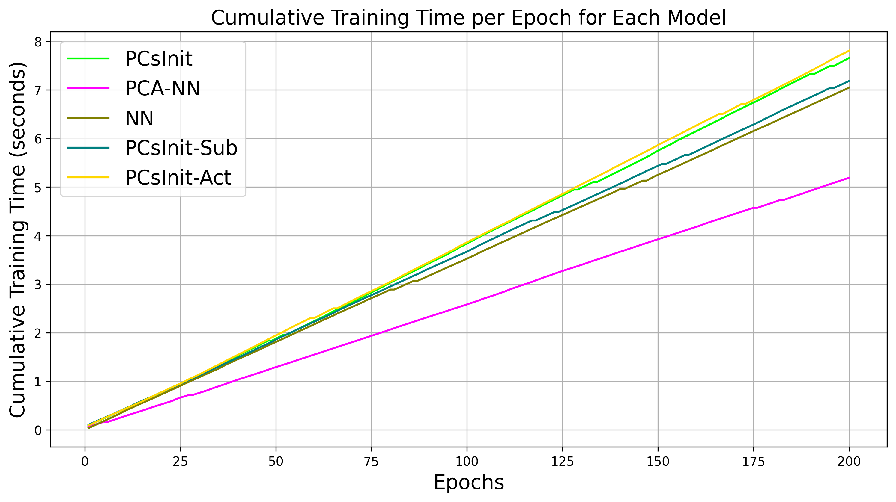
The results demonstrate that PCsInit-Sub achieves competitive performance compared to the full PCsInit method, while significantly reducing computational overhead. Across all datasets, PCsInit-Sub consistently delivers similar levels of accuracy and training loss stability, closely mirroring the trends observed in PCsInit. For example, on the Heart dataset, PCsInit-Sub performs better under He initialization (figure 3), slightly worse under Orthogonal initialization (figure 3), and achieves the same performance under Xavier initialization (3). On the Ionosphere dataset, PCsInit-Sub demonstrates mostly the same performance across all initialization techniques (figures 6, 6, and 6), maintaining its robustness. Additionally, on the Micromass dataset, PCsInit-Sub exhibits more stable and better performance under He initialization (figure 9), while on the Parkinson dataset, it outperforms PCsInit under Xavier initialization (figure 12). This ability to maintain high performance, stability, and reduced computational speed as indicated in figures 14 and 14 highlights the efficiency of PCsInit-Sub, making it an appealing alternative for scenarios with large datasets or limited resources.
Next, the results also show that PCsInit-Act many times can be a more stable and competitive variation compared to the standard PCsInit, with slight improvements observed on the Ionosphere and Micromass datasets across all initialization techniques (figures 6, 6, 6, 9, 9, and 9). This highlights its ability to adapt effectively to varying data structures while maintaining consistent performance. Notably, PCsInit-Act demonstrates exceptional results under the Xavier initialization technique for other layers, emerging as the best-performing approach on three out of the four datasets: Heart, Ionosphere, and Micromass (figures 3, 6, and 9). This consistent superiority under Xavier initialization underscores the robustness of PCsInit-Act in leveraging the initialization method to enhance training stability and accuracy. These findings emphasize the effectiveness of PCsInit-Act, particularly in scenarios requiring both competitive performance and stability.
For datasets with a larger number of features, such as the Micromass dataset where the number of features exceeds the number of samples, the challenges of training are more pronounced. While PCsInit does not achieve exceptional results across all initialization techniques, it still outperforms the standard NN, demonstrating its robustness in handling high-dimensional data. Furthermore, its variations, PCsInit-Act and PCsInit-Sub, exhibit superior performance, offering attractive alternative approaches with enhanced stability and competitive accuracy. These results highlight the adaptability and effectiveness of the proposed methodology, particularly in addressing the complexities of high-dimensional datasets.
V Conclusion
In conclusion, in this work, we propose PCsInit, which initializes the first layer of a neural network with the principal components obtained from the input data and illustrates its advantages compared to training a neural network on principal components. In general, PCsInit and its variations (PCsInit-Sub and PCsInit-Act) not only provide a more direct and easy way to explain the decision of a model but also outperform PCA-NN and NN across various datasets and initialization techniques. We also show theoretically and experimentally that PCsInit and its variants converge faster than NN.
In the future, we will examine the performance of the proposed approaches under various neural network architectures and various types of data (noisy, imbalanced). In addition, we will explore the potential usage of Kernel PCA instead of PCA for initializing neural networks.
References
- [1] Grégoire Montavon, Geneviève Orr, and Klaus-Robert Müller. Neural networks: tricks of the trade, volume 7700. springer, 2012.
- [2] Christopher M Bishop and Nasser M Nasrabadi. Pattern recognition and machine learning, volume 4. Springer, 2006.
- [3] Trevor Hastie, Robert Tibshirani, Jerome H Friedman, and Jerome H Friedman. The elements of statistical learning: data mining, inference, and prediction, volume 2. Springer, 2009.
- [4] Ian T Jolliffe and Jorge Cadima. Principal component analysis: a review and recent developments. Philosophical transactions of the royal society A: Mathematical, Physical and Engineering Sciences, 374(2065):20150202, 2016.
- [5] Marco Tulio Ribeiro, Sameer Singh, and Carlos Guestrin. ” why should i trust you?” explaining the predictions of any classifier. In Proceedings of the 22nd ACM SIGKDD international conference on knowledge discovery and data mining, pages 1135–1144, 2016.
- [6] Matthew D Zeiler and Rob Fergus. Visualizing and understanding convolutional networks. In Computer Vision–ECCV 2014: 13th European Conference, Zurich, Switzerland, September 6-12, 2014, Proceedings, Part I 13, pages 818–833. Springer, 2014.
- [7] Leo Breiman. Random forests. Machine Learning, 45(1):5–32, 2001.
- [8] Timor Kadir and Michael Brady. Saliency, scale and image description. International Journal of Computer Vision, 45(2):83–105, 2001.
- [9] Ramprasaath R Selvaraju, Michael Cogswell, Abhishek Das, Ramakrishna Vedantam, Devi Parikh, and Dhruv Batra. Grad-cam: Visual explanations from deep networks via gradient-based localization. In Proceedings of the IEEE International Conference on Computer Vision, pages 618–626, 2017.
- [10] Scott M Lundberg and Su-In Lee. A unified approach to interpreting model predictions. Advances in neural information processing systems, 30, 2017.
- [11] Azmy S Ackleh, Edward James Allen, R Baker Kearfott, and Padmanabhan Seshaiyer. Classical and modern numerical analysis: Theory, methods and practice. Crc Press, 2009.
- [12] Thu Nguyen, Hoang Thien Ly, Michael Alexander Riegler, and Pål Halvorsen. Principle components analysis based frameworks for efficient missing data imputation algorithms. arXiv preprint arXiv:2205.15150, 2022.
- [13] Vincent Audigier, François Husson, and Julie Josse. Multiple imputation for continuous variables using a bayesian principal component analysis. Journal of statistical computation and simulation, 86(11):2140–2156, 2016.
- [14] Tu T Do, Anh M Vu, Tuan L Vo, Hoang Thien Ly, Thu Nguyen, Steven Hicks, Pål Halvorsen, Michael Riegler, and Binh T Nguyen. Blockwise principal component analysis for monotone missing data imputation and dimensionality reduction. In 2024 International Joint Conference on Neural Networks (IJCNN), pages 1–8. IEEE, 2024.
- [15] Thuong HT Nguyen, Bao Le, Phuc Nguyen, Linh GH Tran, Thu Nguyen, and Binh T Nguyen. Principal components analysis based imputation for logistic regression. In International Conference on Industrial, Engineering and Other Applications of Applied Intelligent Systems, pages 28–36. Springer Nature Switzerland Cham, 2023.