Learning the Hamiltonian Matrix of Large Atomic Systems
Abstract
Graph neural networks (GNNs) have shown promise in learning the ground-state electronic properties of materials, subverting ab initio density functional theory (DFT) calculations when the underlying lattices can be represented as small and/or repeatable unit cells (i.e., molecules and periodic crystals). Realistic systems are, however, non-ideal and generally characterized by higher structural complexity. As such, they require large (10+ Å) unit cells and thousands of atoms to be accurately described. At these scales, DFT becomes computationally prohibitive, making GNNs especially attractive. In this work, we present a strictly local equivariant GNN capable of learning the electronic Hamiltonian () of realistically extended materials. It incorporates an augmented partitioning approach that enables training on arbitrarily large structures while preserving local atomic environments beyond boundaries. We demonstrate its capabilities by predicting the electronic Hamiltonian of various systems with up to 3,000 nodes (atoms), 500,000+ edges, 28 million orbital interactions (nonzero entries of ), and 1% error in the eigenvalue spectra. Our work expands the applicability of current electronic property prediction methods to some of the most challenging cases encountered in computational materials science, namely systems with disorder, interfaces, and defects.
1 Introduction
Graph neural networks (GNNs) have proven capable of learning properties that are functions of molecular and atomic structures, and thus easily represented by graph-structured data (Veličković et al., 2018). They have already enabled new directions of research previously thought computationally unaffordable. More recently, GNNs have been applied to predict electronic-level properties. The most general of such properties is the ground-state Hamiltonian matrix , which, if expressed in a localized basis, can be decomposed into sub-matrices that encode the coupling between the sets of basis elements located on atoms and . These coupling terms depend on the nature (atomic type) and relative coordinates of the local environment.
Previous works on electronic property prediction focused on the cases of molecules (Zhong et al., 2023; Yu et al., 2023b; Bai et al., 2021) and ordered materials (Li et al., 2022; Gong et al., 2023; Wang et al., 2024a) whose graph representations are fairly small; typical molecules contain only a few atoms and all relevant structural information in crystalline materials can be captured by translating a small unit cell. The electronic properties of such systems can be computed “exactly” with density functional theory (DFT) within a few minutes on a single CPU.
Real materials, however, are not made with the repetition of small unit cells. The unavoidable presence of defects, for example, doping atoms, vacancies, strain, compositional variations, or lattice mismatch (Ducry et al., 2020; Kaniselvan et al., 2023; Strand et al., 2018), requires large unit cells composed of up to a few thousand atoms to capture the associated structural disorder (Repa & Fredin, 2023). Accurate DFT simulations of such non-ideal materials are prohibitively expensive, even on today’s largest supercomputers. The prospect of applying machine learning solutions to handle such systems is thus particularly attractive and of high relevance in computational materials science.
Here, we adapt equivariant GNN approaches to learn the ground-state Hamiltonian of this more realistic class of atomic structures. As main contributions:
-
•
We develop a strictly local GNN-based architecture tailored for electronic property prediction from small to large scales. Our network leverages efficient SO(2)-convolutions and multi-headed attention, with learnable embeddings for every node and edge that are mapped to diagonal () and off-diagonal () blocks of the Hamiltonian. We provide the code for this implementation in [anonymized].
-
•
We propose an efficient augmented partitioning method that incorporates virtual nodes/edges to enable partitioning of input graphs while maintaining their exact connectivity. Arbitrarily large graphs can then be decomposed into independent partitions that fit into GPU memory during training without compromising the achievable testing accuracy.
We combine our network and augmented partitioning approach to treat a custom dataset of three large atomic structures in their amorphous phase. As amorphous materials encompass all aforementioned defect types, they are ideally suited to test and validate our model. In particular, we achieve 0.99-5.16 meV prediction accuracies on unseen samples, matching the ranges of previous studies for materials with orders of magnitude fewer atoms (Wang et al., 2024b). We also demonstrate how this error translates into downstream applications by matching the eigenvalues of to within 0.55% relative L1 error on structures with 3,000 atoms, which require several (3.65) hours to compute using DFT. Our work advances applications of equivariant GNNs towards practical use cases in computational materials science.
2 Background & related work
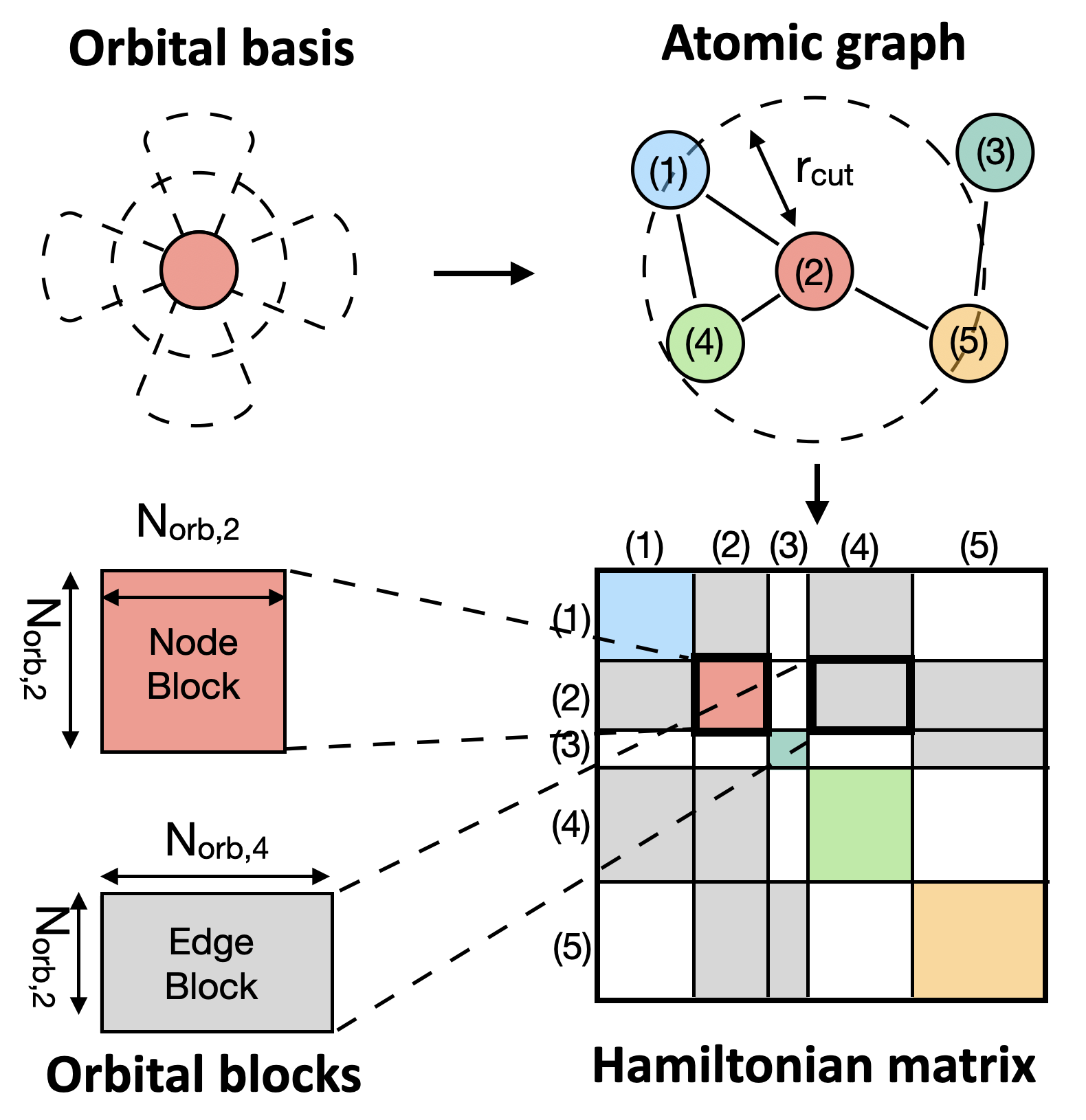
The electronic properties of a material refer to its set of energy levels () and wavefunctions () that electrons can occupy. They correspond to the eigenvalues and eigenvectors of the Hamiltonian matrix describing the atomic system of interest. This quantity is a function of the location (relative positions ) and identity (atomic numbers ) of all constituent atoms ((Hohenberg & Kohn, 1964)). Therefore, predicting the electronic properties of materials consists of learning the mapping between the atomic structure and the elements of the corresponding Hamiltonian matrix, before diagonalizing to obtain and (Fig. 1).
The entries of the ground-state Hamiltonian matrix are typically computed from first principles with DFT ((Kohn & Sham, 1965)). In several widely used codes, the wavefunctions are expanded into a basis of non-orthogonal atomic orbitals localized around atomic positions, each built, for example, from contracted Gaussian functions ((Kühne et al., 2020; Neese, 2011)). These orbitals transform like spherical harmonics under rotation : . Here, is the spherical harmonic of degree and order . is the Wigner-D matrix of degree corresponding to the rotation , which transforms the corresponding spherical harmonic. and are normalized direction vectors.
The localized nature of the basis states leads to finite spatial overlaps between them. The resulting Schrödinger-like equation at the core of DFT takes the form of a generalized eigenvalue problem: . Here, the Hamiltonian matrix has entries where is the so-called Hamiltonian operator. The Overlap matrix is defined as . They are both coarse-grained matrices of size , where is the number of atoms, the number of orbitals per atom, and indices over the different atomic species found in the system. Note that reduces to the identity matrix in case of an orthogonal basis . Otherwise, it can be directly computed from the basis as the problem’s physics does not influence it.
The Hamiltonian matrix can be decomposed into sub-matrices of size , each describing the interactions between all basis elements (orbitals) on atoms and . Diagonal blocks () are the interactions between orbitals on the same atom. When represented on a local basis, the matrix is near-sighted; the interactions between orbitals on different atoms decay exponentially with increasing interatomic distance. Since an atomic orbital basis is used, the sub-matrices are also equivariant under rotation of the atomic bonds, with their transformation properties related by the Wigner-D matrix.
2.1 Challenges unique to disordered materials
Computing the electronic properties of disordered materials with DFT still requires defining a repeatable ‘unit cell’ that is translated through space to construct the desired atomic system. Periodic boundaries are applied to the surface of this cell to avoid dangling bonds. However, the assumed periodicity can alter the disordered nature of the material if the repeating unit cell is too small. If atoms can interact with all their periodic images, non-physical phenomena may arise such as the formation of coherent electronic states across cells, drastically affecting the material properties. Small unit cells thus cannot accurately represent the physics of disordered systems. To avoid such unrealistic scenarios and better approximate disorder, ‘large-enough’ unit cells should be constructed, with dimensions ranging from 10 Å (Repa & Fredin, 2023) to a few nanometers (Ducry et al., 2020). Generating the Hamiltonian matrix of these systems with DFT involves tens to hundreds of self-consistent field (SCF) loops, each requiring the diagonalization of an intermediate , the solution of Poisson’s equation, and the creation of a new Hamiltonian matrix. As the first operation scales with , analyzing electronic properties for large disordered systems (or different representations of disorder for the same material) is often computationally unaffordable.
2.2 Hamiltonian prediction models
Only a few studies have attempted to directly predict the Hamiltonian matrix of a given material with a GNN rather than fitting its invariant quantities such as the total energy. The key is to constrain the solution space by leveraging prior knowledge of physical symmetries, e.g., rotational equivariance of orbital blocks.
In such equivariant GNNs, the predicted Hamiltonian rotates along with the input (Yu et al., 2023b; Zhang et al., 2024; Batatia et al., 2023; Gong et al., 2023), which requires maintaining SO(3)-equivariance within the model. In other words, all network operations acting on input embedding of degree must satisfy: . The resulting networks are trained using Message Passing (MP), where each MP layer works as follows: An atom receives input messages from all its neighboring source atoms . Each input message goes through convolution operations that combine features with different while preserving equivariance; a specific output embedding of degree can be computed through: . Here, is a normalized vector indicating the direction of the edge connecting the atoms and , and is a set of trainable weights. The sum runs over tensor products which take (a source input embedding of degree ) and (a filter spherical harmonic embedding of degree ) and produce the output embedding:
where the are the Clebsch-Gordan coefficients that are indexed by the order and degree of the input, filter, and output embeddings. The combination of feature () and geometric () information along each edge encodes both the identity and structure of the system. These ‘Tensor Field Networks’ (TFNs) (Hodapp & Shapeev, 2023) achieve state-of-the-art accuracy on small molecule (Yu et al., 2023b) and crystalline (Gong et al., 2023) datasets. However, they are also computationally expensive. The network training scales with , where is the maximum degree of the angular momentum considered. As a consequence, E(3)-equivariant tensor product networks are difficult to apply beyond a few atoms (Zhang et al., 2024).
Recently, the computational cost of training equivariant GNNs has been significantly reduced by combining the benefits of data rotation and equivariant network operations. These approaches take advantage of the fact that when edges are rotated to align with a fixed axis ( or depending on convention), the only non-zero spherical harmonic components are those of order = 0. By keeping track of the bond vectors and performing internal spherical rotations, complex SO(3) convolutions can thus be reduced to SO(2) linear convolution operations (Passaro & Zitnick, 2023). Furthermore, under these conditions, the Clebsch-Gordan coefficients exhibit a predictable sparsity pattern (non-zero only when = ). Altogether, the scaling reduces to (Wang et al., 2024a), thus speeding up the network’s training, while enabling the use of higher-order angular momenta () and more parameters to capture finer, more complex details of the surrounding environment. An advanced SO(2) convolution network was developed by (Passaro & Zitnick, 2023) (eSCN), while an implementation of this approach on Hamiltonians by (Wang et al., 2024a) achieved better performance on custom crystalline 2D-material datasets compared to previous tensor field and invariant networks. The architecture was further expanded by (Liao et al., 2023) (EquiformerV2) with the inclusion of equivariant attention. However, the prediction of large disordered structures still remains an open problem in literature.
3 Methods
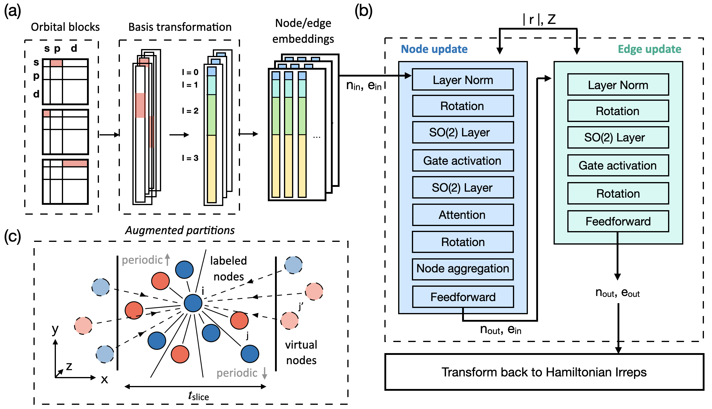
We first present an equivariant architecture that is custom-made for large-scale Hamiltonian prediction. A high-level overview is shown in Fig. 3(a)-(b). Relevant implementation details and ablation studies are presented in Section 4 and Appendix B.
3.1 Orbital block processing
Each block of the Hamiltonian matrix represents the interaction (coupling) between the spherical harmonics of degree on atom and that of degree on atom . Mathematically, it can be cast into the tensor product of length between the uncoupled angular momentum eigenstates and . Each of these tensor products can be decomposed into a direct sum () of coupled angular momentum eigenstates , where ranges from to : . The transformation from the uncoupled to the coupled basis is performed using a matrix of Clebsch-Gordon coefficients. For example, the coefficient for a specific coupled angular momentum eigenstate component is given by:
Applying a rotation to the resulting then consists of independently applying the corresponding Wigner-D transformation () to each of its subspaces of degree . To minimize the number of transformations, all orbital blocks are initially transformed into the coupled basis as a pre-processing step (Fig. 3(a)).
3.2 Network architecture
The graph’s nodes/edges are first initialized with embeddings of shape (, , )/(, , ), where is the number of nodes/edges, the dimension of the node/edge embeddings, and the maximum degree of the features. The channels of the node embeddings are initialized with atomic numbers, while those of the edge embeddings are initialized with the scalar distance between the two connecting nodes, expanded in the chosen basis, here, contracted Gaussian functions. All other components are initially set to 0.
During the node update phase, each node receives messages from all its neighbors , consisting of the concatenated embeddings , , and . To enable fast tensor product operations in large atomic structures, we adopt eSCN convolutions (Passaro & Zitnick, 2023), with incoming messages rotated to align with the -axis during these operations. Non-linearity is then introduced through a gate activation layer. On top of this, we also include dynamic multi-headed attention mechanisms, as in EquiformerV2 (Liao et al., 2023), which allows our network to learn better from highly dense local atomic environments. Finally, the resulting output messages are rotated back to their original orientations, aggregated onto the node , and passed through a feedforward network to update its output embedding corresponding to onsite (diagonal) Hamiltonian blocks.
To learn offsite (non-diagonal) blocks, we use concepts from the Hamiltonian prediction networks in (Gong et al., 2023),(Wang et al., 2024a) and introduce learnable embeddings for every edge, defined between pairs of atoms located within a distance rcut from each other. The updated node embeddings are used to update the edges through a similar process, without the attention layer. The predicted outputs are then post-processed back into the uncoupled basis with the reverse transformation: = , such that they can be used to reconstruct the Hamiltonian matrix block-by-block.
3.3 Training on augmented partitions
A notable difference between our application and that of standard GNNs in computational materials resides in the density of interatomic interactions. Many types of physical interactions are short-range and can be captured with a limited receptive field (Batatia et al., 2025). However, despite the near-sightedness property of Gaussian functions, orbitals located on different atoms can interact with each other over distances exceeding 10 Å (see Appendix F), giving rise to specific nonzero off-diagonal blocks in the Hamiltonian matrix. They must be taken into account by increasing rcut. The graph representation of these structures is thus densely connected, with edges per node.
The combination of large graphs, dense connectivity, and large tensor representations of nodes and edges, results in high memory consumption and long computation times per epoch during training (see Appendix H.2). If a distributed computing environment was used, the communication of intermediate values during the forward pass would incur significant overhead, impeding scalability (Wan et al., 2022). At the same time, graphs cannot be arbitrarily partitioned by removing inter-atomic connections. Doing so misinforms the network as it tries to fit the target data while aggregating inputs through an incorrect/incomplete graph structure. The inability to divide the graph into batches slows down the training process overall.
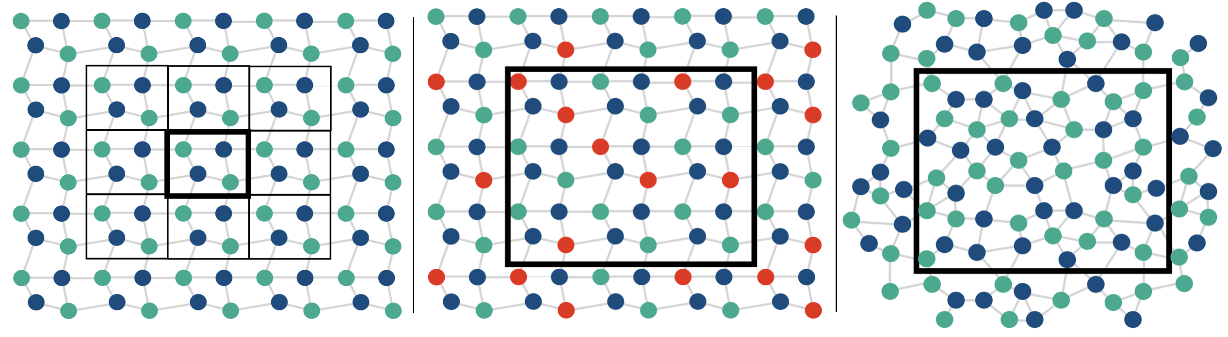
To efficiently train graphs corresponding to large materials while maintaining correct atomic environments and neighboring edge connections, we introduce an augmented partitioning approach. A visual representation of it is provided in Fig. 3(c). The graph is first partitioned into sub-graphs where the data can fit into the memory of a single GPU. Atoms located outside of a given partition, but connected to those within, are represented by virtual nodes (Fig. 3(c) - dashed circles). They are attached to the partition through virtual edges (Fig. 3(c) - dashed lines). These virtual nodes/edges are initialized similarly to their labeled counterparts with input atomic numbers and distances. However, their outputs are not used. Their only purpose is to inform each partition of its full connectivity so that the network can then learn an accurate and generalizable aggregation function during message passing. To leverage the periodic boundaries of the material structures treated here, we partition the input structures by dividing the graph into ‘slices’ along the longest dimension (-axis), retaining edges across the - and -boundaries. Details about the construction of partitions are provided in Appendix B.
As the set of virtual connections used to augment each graph includes only the 1-hop neighborhood, the network is strictly local. Limiting the receptive field is an approach often used to increase scalability. As demonstrated by previous strictly local architectures, e.g., Allegro (Musaelian et al., 2023), information from the local environment is often sufficient to achieve state-of-the-art prediction accuracy when interactions are strongly localized and the interaction cutoff is sufficiently large. In Appendix F, we present further details on how the Hamiltonian matrix elements satisfy this locality. To capture higher body-order information, many-body interactions can be flexibly added into the network without increasing the receptive field, as implemented by (Zhouyin et al., 2024).
3.4 Dataset creation
| Material | Structure | Purpose | [Å] | # atoms | # orbitals | # edges | [Å] | [Å] | [Å] |
|---|---|---|---|---|---|---|---|---|---|
| a-HfO2 | 1 | validate | 8 | 3,000 | 18,000 | 527,348 | 52.876 | 26.308 | 26.242 |
| a-HfO2 | 2 | train | 8 | 3,000 | 18,000 | 533,364 | 52.346 | 26.237 | 26.293 |
| a-HfO2 | 3 | test | 8 | 3,000 | 18,000 | 530,920 | 52.722 | 26.267 | 26.191 |
| a-GST | 1 | train/validate (6:1 split) | 12 | 1,008 | 13,104 | 230,848 | 29.541 | 25.583 | 41.777 |
| a-GST | 2 | test | 12 | 1,008 | 13,104 | 226,406 | 25.857 | 29.857 | 41.691 |
| a-PtGe | 1 | train/validate (10:1 split) | 8 | 2,688 | 16,128 | 319,262 | 82.283 | 23.171 | 25.031 |
| a-PtGe | 2 | test | 8 | 2,688 | 16,128 | 319,306 | 82.283 | 23.171 | 25.031 |
| a-PtGe | 2 | test | 16 | 2,688 | 16,128 | 2,154,506 | 82.283 | 23.171 | 25.031 |
To generate sufficiently rich training data, existing datasets typically sample molecules at various time steps of molecular dynamics (MD) trajectories (Yu et al., 2023a; Schütt et al., 2019; Christensen & lilienfeld, 2020) or generate multiple small perturbations of the atoms in a crystalline lattice (Li et al., 2022). Here, as a representative subset of realistic (disordered) materials, we consider amorphous crystals and take advantage of the fact that (1) every node has a different local atomic environment, and (2) each structure contains a large sampling of different motifs. A wide range of training data can thus be captured within a single sample.
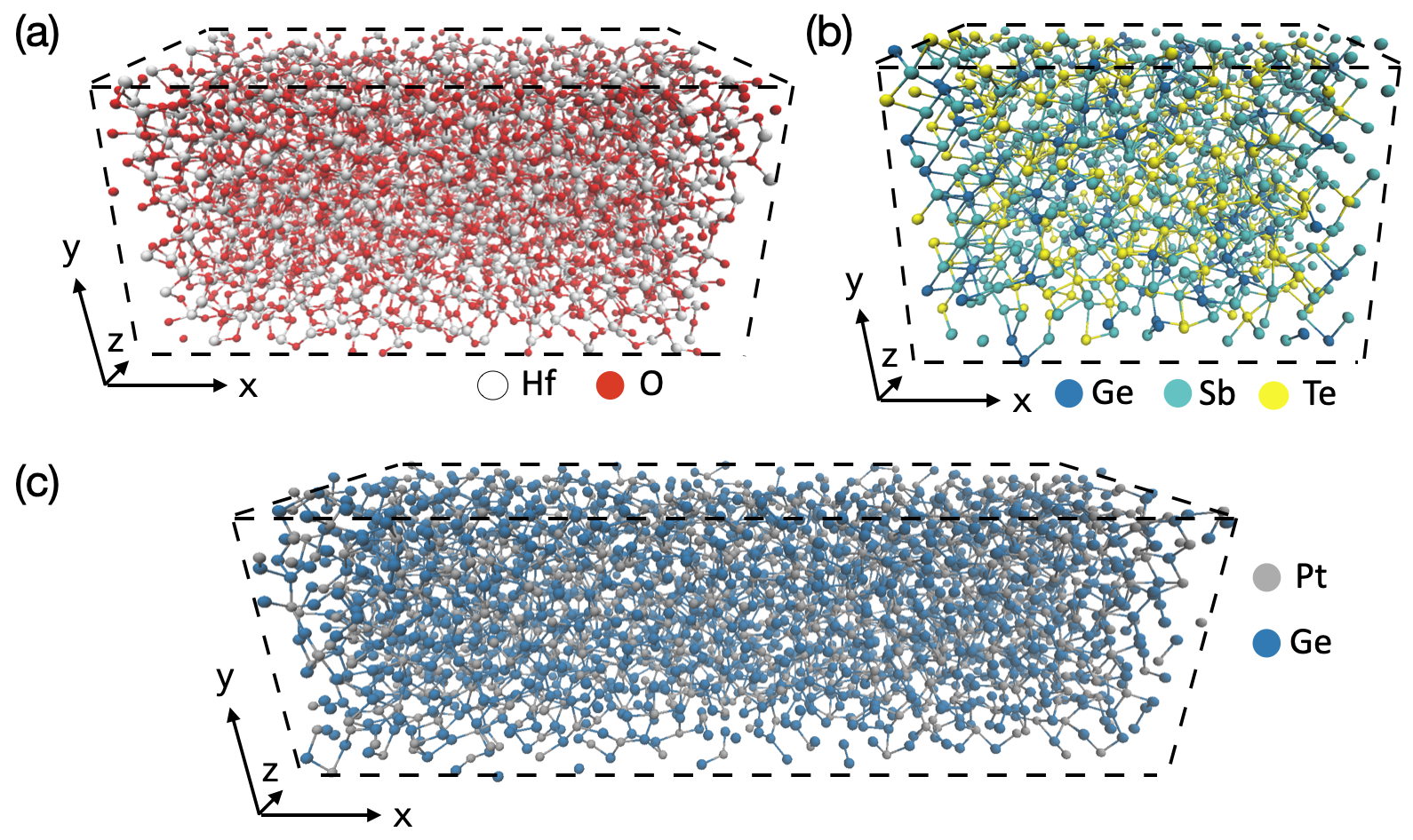
We generate a custom dataset for three different materials in the amorphous (a-) phase (without long-range order): a-HfO2, a-GeSbTe (a-GST), and a-PtGe. Besides exhibiting features that require large unit cells to be described, these materials are also scientifically and technologically relevant: a-HfO2 is a common high- dielectric that can be found in almost all transistors and integrated circuits (Chan et al., 2008). a-GST and alloys of a-Ge show high resistance contrasts between crystalline and amorphous phases, and can be used as switching layers of non-volatile memory cells (Pirovano et al., 2004; Kolobov et al., 2004; Zellweger et al., 2024) that are fully compatible with CMOS fabrication processes. Knowing the electronic Hamiltonian of these materials is essential to understanding the behavior of the corresponding devices and to designing better-performing components (Brandbyge et al., 2002). Structure examples can be visualized in Fig. 4 for each material. The corresponding structural information used for training, validation, and testing is found in Table 1. Details behind the sample generation are given in Appendix D. This dataset will be made publicly available to serve as a reference for large electronic Hamiltonian matrix predictions.
4 Results
For fair comparisons in experiments where the quantity of training data may vary, we used a ReduceLRonPlateau scheduler that reduces the learning rate when no further decrease in validation loss is detected. Training is stopped once a minimum learning rate is reached. The values of the hyperparameters and the scheduler settings for different experiments are discussed in Appendix C.
4.1 Ablation studies of the training approach
We study the model’s ability to generalize to different configurations of large systems by predicting the Hamiltonian matrix of a full a-HfO2 sample (structure 3 in Table 1), which remains unseen during the training process. For all subsequent HfO2 experiments, the augmented partitioning scheme is only applied during training on structure 2, while the of the full unseen structure is predicted during inference (structure 3). We use an rcut of 8 Å. Errors are reported separately for nodes () and edges () to distinguish intra- and inter-atomic orbital interactions, which have very different magnitudes.
| 5.18 | 1.66 | ||
| 2.29 | 0.20 |
First, we demonstrate the improvement in accuracy resulting from the augmented partitioning approach introduced in Section 3.3. In particular, we examine the influence of virtual nodes/edges in Table 2. Compared to training with raw partitions, the addition of virtual nodes and edges reduces the node () and edge prediction error () by 50% and 88% respectively. Such an improvement is expected, as raw partitions omit a large proportion of boundary edges and thus incorrectly capture atomic neighborhoods. We note that as , the one-hop neighborhood connects all nodes within each partition.
Next, we explore the impact of augmented partitioning on accuracy by training on an increasingly sub-divided graph in Table 3. The total number of labeled atoms used for training remains the same (3,000), while the total number of labeled edges decreases with more partitions. Despite the different divisions ranging from 5 (12 Å) to 27 (2 Å) slices, and remain very close to the values obtained by training with the full graph ( = 52.346 Å). The prediction error is thus insensitive to partition size. Using multiple partitions also allows for effective batching, reducing the number of epochs required for convergence. For small slices, the reduced fraction of labeled connections along the direction does not affect the accuracy, as the remaining data along the and directions is sufficient to train the network.
| [Å] | Epochs | ||||
|---|---|---|---|---|---|
| 2 | 27 | 95,398 | 15,790 | 2.35 | 0.20 |
| 3 | 18 | 141,512 | 18,990 | 2.15 | 0.18 |
| 4 | 14 | 184,730 | 17,098 | 2.32 | 0.19 |
| 8 | 7 | 320,324 | 20,599 | 2.37 | 0.17 |
| 12 | 5 | 381,504 | 19,351 | 2.69 | 0.18 |
| 52 | 1 | 533,364 | 23,396 | 2.46 | 0.16 |
4.2 Structural disorder
We apply the same local architecture to our custom dataset of structurally disordered (amorphous) materials (HfO2, GST, and PtGe from Fig. 4/Table 1), which contain a range of different atomic elements (Hf, O, Ge, Sb, Te, Pt), basis sets (SZV, DZVP), and bonding behavior (ionic, covalent). All models are trained using augmented partitions and tested on full unseen structures belonging to the same material. The results are summarized in Table 4.
| Material | [Å] | [Å] | |||||||
|---|---|---|---|---|---|---|---|---|---|
| a-GST | 5 | 6 | 12 | 1,008 | 226,406 | 0.97 | 0.10 | 0.10 | 2.77 |
| a-PtGe | 5 | 10 | 8 | 2,688 | 319,306 | 0.78 | 0.08 | 0.09 | 2.39 |
| a-PtGe | 5 | 10 | 16 | 2,688 | 2,154,506 | 0.82 | 0.04 | 0.04 | 0.99 |
| a-HfO2 | 3 | 18 | 8 | 3,000 | 530,920 | 2.15 | 0.18 | 0.19 | 5.16 |
The strictly local architecture combined with augmented partitioning performs consistently across a diverse range of test datasets, with total errors ranging from 0.99 meV to 5.16 meV, for test structures containing 1000-3000 atoms and 200,000+ to 2,000,000+ edges. These values are comparable to what a previous study obtained (2.2 ) using equivariant GNNs for smaller structures with 150 atoms per unit cell (Wang et al., 2024b). In all cases, the prediction errors also remain relatively insensitive to the partition size (Table 11 in Appendix I). In the case of PtGe, the use of small slices enables to push to 16 Å and remain within GPU memory limitations, further improving prediction accuracy. The error can be further reduced with more training data (Table 9 in Appendix I).
4.3 Compositional disorder
a-HfO2 often exists in a sub-stoichiometric form (a-HfOx) due to the presence of oxygen vacancies induced by the growth process. The distribution of these vacancies varies significantly from one sample to the other, introducing a statistical component to computational studies of the HfOx electronic properties. Accounting for these compositional variations necessitates a distinct DFT simulation for each stoichiometric different structure, which is computationally intensive, but an ideal application of machine learning solutions.
To demonstrate our network’s ability to treat such problems, we train a model on a single sub-stoichiometric a-HfO1.8 structure where 10% of the oxygen atoms were replaced by randomly distributed vacancies represented as ghost atoms. We then use it to predict unseen full structures with a stoichiometry of a-HfO1.7, a-HfO1.8, and a-HfO1.9. The and remain within a small range (2.48-2.60 and 0.17-0.18 , respectively), regardless of the vacancy concentration and distribution, showing that the network generalizes very well to compositional disorder, despite being trained on only one configuration. Models trained on other vacancy concentrations perform similarly. Their results, along with details of the vacancy implementation, can be found in Appendix I.2.
| Stoichiometry () | |||
|---|---|---|---|
| Train set | Test set | ||
| 1.8 | 1.9 | 2.48 | 0.18 |
| 1.8 | 1.8 | 2.50 | 0.17 |
| 1.8 | 1.7 | 2.60 | 0.18 |
4.4 Eigenvalue spectrum of predicted a-HfO2
Next, we assess whether the prediction accuracy of the trained network is sufficient for practical application. For this, we use HfO2, as it has the highest error in our experiments in Table 4 and thus presents an upper bound on the expected accuracy. We assemble the full Hamiltonian of the HfO2 test structure using the network outputs (), trained with 18 partitions of length = 3 Å. We then compute the eigenvalue spectrum of and its reference , as well as the error distribution between them (Fig. 5(a)). The predicted is able to reproduce all eigenvalues of within 0.550% relative L1 error. The error decreases to 0.487% when eigenvalues of unoccupied states (those situated above 0.306 ) are excluded. The remaining error is carried mostly by the largest eigenvalues and distributed around the edges of energy gaps (see Fig. 8 in Appendix F), which correspond to regimes of stronger inter-atomic orbital coupling (Atkins & De Paula, 2009).

4.5 Computational cost
Compared to full-batch training of the graph, our method using 8 augmented slices results in a 6.5 speedup per epoch (0.38 vs. 2.5 s) and a 7.2 decrease in memory consumption per rank (8.59 vs. 61.68 GiB) without affecting accuracy. A more complete analysis is provided in Appendix H.2. This scaling behavior is only limited by the overhead introduced to process the virtual nodes/edges and by any computational load imbalance from partitioning. Further computational improvements could be achieved by combining the augmentation approach with optimized graph partitioning algorithms extended to leverage periodicity.
The extension of GNN-based predictions to large material systems could potentially save tremendous amounts of computational time, as the inference phase scales with while DFT calculations are limited to . While DFT calculations to obtain the of small molecules (e.g., H2O) take only a few seconds, the same operation for a-HfO2 structures made of 3,000 atoms is computationally two orders of magnitude heavier (0.04 vs. 3.65 node hours, see Appendix H). We have thus demonstrated the applicability of GNN approaches to a regime where exact solutions are almost entirely prohibitive for downstream applications. The model could also serve as an initial guess to DFT packages to reduce the number of self-consistent field iterations that are required to obtain converged electron densities (Unke et al., 2021).
5 Conclusion
We developed an equivariant GNN tailored to learn the electronic properties of large-scale, disordered materials, and introduced an augmented partitioning approach to break down and train the graphs encountered when dealing with realistic materials, without sacrificing accuracy. More generally, we proposed a method to tackle the training of systems represented by large, highly connected, and near-sighted graphs where a strictly local environment is sufficient. Our approach can be straightforwardly applied to other complex materials, or adapted to learn their other rotationally-equivariant attributes, such as vibrational properties, e.g., phonon dispersions (Fang et al., 2024). The resulting network captures relevant properties of large structures in sufficient detail to achieve few- accuracy and reproduce the energy eigenvalues to under 0.6% error. Further data generation, network optimization, and enabling increased expressiveness will be the next steps.
References
- Anisimov et al. (1991) Anisimov, V. I., Zaanen, J., and Andersen, O. K. Band theory and mott insulators: Hubbard u instead of stoner i. Physical Review B, 44:943–954, Jul 1991.
- Atkins & De Paula (2009) Atkins, P. and De Paula, J. Atkins’ physical chemistry. Oxford University Press, London, England, 9 edition, November 2009.
- Bai et al. (2021) Bai, H., Chu, P., Tsai, J.-Y., Wilson, N., Qian, X., Yan, Q., and Ling, H. Graph neural network for hamiltonian-based material property prediction. Neural Computing and Applications, 34(6):4625–4632, November 2021. ISSN 1433-3058. doi: 10.1007/s00521-021-06616-0. URL http://dx.doi.org/10.1007/s00521-021-06616-0.
- Batatia et al. (2023) Batatia, I., Schaaf, L. L., Chen, H., Csányi, G., Ortner, C., and Faber, F. A. Equivariant matrix function neural networks, 2023. URL https://arxiv.org/abs/2310.10434.
- Batatia et al. (2025) Batatia, I., Batzner, S., Kovács, D. P., Musaelian, A., Simm, G. N. C., Drautz, R., Ortner, C., Kozinsky, B., and Csányi, G. The design space of e(3)-equivariant atom-centred interatomic potentials. Nature Machine Intelligence, 7(1):56–67, January 2025. ISSN 2522-5839. doi: 10.1038/s42256-024-00956-x. URL http://dx.doi.org/10.1038/s42256-024-00956-x.
- Brandbyge et al. (2002) Brandbyge, M., Mozos, J.-L., Ordejón, P., Taylor, J., and Stokbro, K. Density-functional method for nonequilibrium electron transport. Physical Review B, 65(16), March 2002. ISSN 1095-3795. doi: 10.1103/physrevb.65.165401. URL http://dx.doi.org/10.1103/PhysRevB.65.165401.
- Chan et al. (2008) Chan, M., Zhang, T., Ho, V., and Lee, P. Resistive switching effects of hfo2 high-k dielectric. Microelectronic Engineering, 85(12):2420–2424, December 2008. ISSN 0167-9317. doi: 10.1016/j.mee.2008.09.021. URL http://dx.doi.org/10.1016/j.mee.2008.09.021.
- Christensen & lilienfeld (2020) Christensen, A. S. and lilienfeld, A. V. Revised MD17 dataset (rMD17). 7 2020. doi: 10.6084/m9.figshare.12672038.v3. URL https://figshare.com/articles/dataset/Revised_MD17_dataset_rMD17_/12672038.
- Ducry et al. (2020) Ducry, F., Aeschlimann, J., and Luisier, M. Electro-thermal transport in disordered nanostructures: a modeling perspective. Nanoscale Advances, 2(7):2648–2667, 2020. ISSN 2516-0230. doi: 10.1039/d0na00168f. URL http://dx.doi.org/10.1039/d0na00168f.
- Fang et al. (2024) Fang, S., Geiger, M., Checkelsky, J. G., and Smidt, T. Phonon predictions with e(3)-equivariant graph neural networks, 2024. URL https://arxiv.org/abs/2403.11347.
- Gong et al. (2023) Gong, X., Li, H., Zou, N., Xu, R., Duan, W., and Xu, Y. General framework for e(3)-equivariant neural network representation of density functional theory hamiltonian. Nature Communications, 14(1), May 2023. ISSN 2041-1723. doi: 10.1038/s41467-023-38468-8. URL http://dx.doi.org/10.1038/s41467-023-38468-8.
- Hodapp & Shapeev (2023) Hodapp, M. and Shapeev, A. Equivariant tensor networks, 2023. URL https://arxiv.org/abs/2304.08226.
- Hohenberg & Kohn (1964) Hohenberg, P. and Kohn, W. Inhomogeneous electron gas. Physical Review, 136(3B):B864–B871, November 1964. ISSN 0031-899X. doi: 10.1103/physrev.136.b864. URL http://dx.doi.org/10.1103/PhysRev.136.B864.
- Jain et al. (2013) Jain, A., Ong, S. P., Hautier, G., Chen, W., Richards, W. D., Dacek, S., Cholia, S., Gunter, D., Skinner, D., Ceder, G., and Persson, K. A. Commentary: The materials project: A materials genome approach to accelerating materials innovation. APL Materials, 1(1):011002, 07 2013. ISSN 2166-532X. doi: 10.1063/1.4812323. URL https://doi.org/10.1063/1.4812323.
- Kaniselvan et al. (2023) Kaniselvan, M., Luisier, M., and Mladenović, M. An atomistic model of field-induced resistive switching in valence change memory. ACS Nano, 17(9):8281–8292, March 2023. ISSN 1936-086X. doi: 10.1021/acsnano.2c12575. URL http://dx.doi.org/10.1021/acsnano.2c12575.
- Kohn & Sham (1965) Kohn, W. and Sham, L. J. Self-consistent equations including exchange and correlation effects. Physical Review, 140(4A):A1133–A1138, November 1965. ISSN 0031-899X. doi: 10.1103/physrev.140.a1133. URL http://dx.doi.org/10.1103/PhysRev.140.A1133.
- Kolobov et al. (2004) Kolobov, A. V., Fons, P., Frenkel, A. I., Ankudinov, A. L., Tominaga, J., and Uruga, T. Understanding the phase-change mechanism of rewritable optical media. Nature Materials, 3(10):703–708, September 2004. ISSN 1476-4660. doi: 10.1038/nmat1215. URL http://dx.doi.org/10.1038/nmat1215.
- Kühne et al. (2020) Kühne, T. D., Iannuzzi, M., Ben, M. D., Rybkin, V. V., Seewald, P., Stein, F., Laino, T., Khaliullin, R. Z., Schütt, O., Schiffmann, F., Golze, D., Wilhelm, J., Chulkov, S., Bani-Hashemian, M. H., Weber, V., Borštnik, U., Taillefumier, M., Jakobovits, A. S., Lazzaro, A., Pabst, H., and et al. CP2k: An electronic structure and molecular dynamics software package - quickstep: Efficient and accurate electronic structure calculations. J. Chem. Phys., 152(19):194103, May 2020.
- Li et al. (2022) Li, H., Wang, Z., Zou, N., Ye, M., Xu, R., Gong, X., Duan, W., and Xu, Y. Deep-learning density functional theory hamiltonian for efficient ab initio electronic-structure calculation. Nature Computational Science, 2(6):367–377, June 2022. ISSN 2662-8457. doi: 10.1038/s43588-022-00265-6. URL http://dx.doi.org/10.1038/s43588-022-00265-6.
- Li et al. (2020) Li, S., Zhao, Y., Varma, R., Salpekar, O., Noordhuis, P., Li, T., Paszke, A., Smith, J., Vaughan, B., Damania, P., and Chintala, S. Pytorch distributed: Experiences on accelerating data parallel training, 2020. URL https://arxiv.org/abs/2006.15704.
- Liao et al. (2023) Liao, Y.-L., Wood, B., Das, A., and Smidt, T. Equiformerv2: Improved equivariant transformer for scaling to higher-degree representations, 2023. URL https://arxiv.org/abs/2306.12059.
- Musaelian et al. (2023) Musaelian, A., Batzner, S., Johansson, A., Sun, L., Owen, C. J., Kornbluth, M., and Kozinsky, B. Learning local equivariant representations for large-scale atomistic dynamics. Nature Communications, 14(1):579, 2023.
- Neese (2011) Neese, F. The orca program system. WIREs Computational Molecular Science, 2(1):73–78, June 2011. ISSN 1759-0884. doi: 10.1002/wcms.81. URL http://dx.doi.org/10.1002/wcms.81.
- Nordlund et al. (1998) Nordlund, K., Ghaly, M., Averback, R. S., Caturla, M., Diaz de la Rubia, T., and Tarus, J. Defect production in collision cascades in elemental semiconductors and fcc metals. Phys. Rev. B, 57:7556–7570, Apr 1998. doi: 10.1103/PhysRevB.57.7556. URL https://link.aps.org/doi/10.1103/PhysRevB.57.7556.
- Passaro & Zitnick (2023) Passaro, S. and Zitnick, C. L. Reducing so(3) convolutions to so(2) for efficient equivariant gnns, 2023. URL https://arxiv.org/abs/2302.03655.
- Perdew et al. (1997) Perdew, J. P., Burke, K., and Ernzerhof, M. Generalized gradient approximation made simple [phys. rev. lett. 77, 3865 (1996)]. Phys. Rev. Lett., 78:1396–1396, Feb 1997.
- Pirovano et al. (2004) Pirovano, A., Lacaita, A., Benvenuti, A., Pellizzer, F., and Bez, R. Electronic switching in phase-change memories. IEEE Transactions on Electron Devices, 51(3):452–459, March 2004. ISSN 0018-9383. doi: 10.1109/ted.2003.823243. URL http://dx.doi.org/10.1109/TED.2003.823243.
- Repa & Fredin (2023) Repa, G. M. and Fredin, L. A. Predicting electronic structure of realistic amorphous surfaces. Advanced Theory and Simulations, 6(11), June 2023. ISSN 2513-0390. doi: 10.1002/adts.202300292. URL http://dx.doi.org/10.1002/adts.202300292.
- Schütt et al. (2019) Schütt, K. T., Gastegger, M., Tkatchenko, A., Müller, K.-R., and Maurer, R. J. Unifying machine learning and quantum chemistry with a deep neural network for molecular wavefunctions. Nature Communications, 10(1), November 2019. ISSN 2041-1723. doi: 10.1038/s41467-019-12875-2. URL http://dx.doi.org/10.1038/s41467-019-12875-2.
- Senent & Wilson (2001) Senent, M. L. and Wilson, S. Intramolecular basis set superposition errors. International Journal of Quantum Chemistry, 82(6):282–292, 2001. doi: https://doi.org/10.1002/qua.1030. URL https://onlinelibrary.wiley.com/doi/abs/10.1002/qua.1030.
- Stillinger & Weber (1985) Stillinger, F. H. and Weber, T. A. Computer simulation of local order in condensed phases of silicon. Phys. Rev. B, 31:5262–5271, Apr 1985. doi: 10.1103/PhysRevB.31.5262. URL https://link.aps.org/doi/10.1103/PhysRevB.31.5262.
- Strand et al. (2018) Strand, J., Kaviani, M., Gao, D., El-Sayed, A.-M., Afanas’ev, V. V., and Shluger, A. L. Intrinsic charge trapping in amorphous oxide films: status and challenges. Journal of Physics: Condensed Matter, 30(23):233001, May 2018. ISSN 1361-648X. doi: 10.1088/1361-648x/aac005. URL http://dx.doi.org/10.1088/1361-648X/aac005.
- Søren Smidstrup et al. (2020) Søren Smidstrup, K. S., Blom, A., Markussen, T., Wellendorff, J., Schneider, J., Gunst, T., Verstichel, B., Khomyakov, P. A., Vej-Hansen, U. G., Brandbyge, M., et al. Quantumatk: An integrated platform of electronic and atomic-scale modelling tools. J. Phys: Condens. Matter (APS), 32:015901, 2020. doi: 10.1088/1361-648X/ab4007. URL https://iopscience.iop.org/article/10.1088/1361-648X/ab4007.
- Tafen & Drabold (2003) Tafen, D. N. and Drabold, D. A. Realistic models of binary glasses from models of tetrahedral amorphous semiconductors. Physical Review B, 68(16), October 2003. ISSN 1095-3795. doi: 10.1103/physrevb.68.165208. URL http://dx.doi.org/10.1103/PhysRevB.68.165208.
- Thompson et al. (2022) Thompson, A. P., Aktulga, H. M., Berger, R., Bolintineanu, D. S., Brown, W. M., Crozier, P. S., in ’t Veld, P. J., Kohlmeyer, A., Moore, S. G., Nguyen, T. D., Shan, R., Stevens, M. J., Tranchida, J., Trott, C., and Plimpton, S. J. LAMMPS - a flexible simulation tool for particle-based materials modeling at the atomic, meso, and continuum scales. Comp. Phys. Comm., 271:108171, 2022. doi: 10.1016/j.cpc.2021.108171.
- Unke et al. (2021) Unke, O. T., Bogojeski, M., Gastegger, M., Geiger, M., Smidt, T., and Müller, K.-R. Se(3)-equivariant prediction of molecular wavefunctions and electronic densities, 2021. URL https://arxiv.org/abs/2106.02347.
- Urquiza et al. (2021) Urquiza, M. L., Islam, M. M., van Duin, A. C. T., Cartoixà, X., and Strachan, A. Atomistic insights on the full operation cycle of a hfo2-based resistive random access memory cell from molecular dynamics. ACS Nano, 15(8):12945–12954, July 2021. ISSN 1936-086X. doi: 10.1021/acsnano.1c01466. URL http://dx.doi.org/10.1021/acsnano.1c01466.
- VandeVondele & Hutter (2007) VandeVondele, J. and Hutter, J. Gaussian basis sets for accurate calculations on molecular systems in gas and condensed phases. J. Chem. Phys., 127(11):114105, 09 2007. ISSN 0021-9606.
- Veličković et al. (2018) Veličković, P., Cucurull, G., Casanova, A., Romero, A., Liò, P., and Bengio, Y. Graph Attention Networks. In ICLR, 2018.
- Wan et al. (2022) Wan, C., Li, Y., Wolfe, C. R., Kyrillidis, A., Kim, N. S., and Lin, Y. PipeGCN: Efficient full-graph training of graph convolutional networks with pipelined feature communication. March 2022.
- Wang et al. (2024a) Wang, Y., Li, H., Tang, Z., Tao, H., Wang, Y., Yuan, Z., Chen, Z., Duan, W., and Xu, Y. Deeph-2: Enhancing deep-learning electronic structure via an equivariant local-coordinate transformer, 2024a. URL https://arxiv.org/abs/2401.17015.
- Wang et al. (2024b) Wang, Y., Li, Y., Tang, Z., Li, H., Yuan, Z., Tao, H., Zou, N., Bao, T., Liang, X., Chen, Z., Xu, S., Bian, C., Xu, Z., Wang, C., Si, C., Duan, W., and Xu, Y. Universal materials model of deep-learning density functional theory hamiltonian. Science Bulletin, 69(16):2514–2521, 2024b. ISSN 2095-9273. doi: https://doi.org/10.1016/j.scib.2024.06.011. URL https://www.sciencedirect.com/science/article/pii/S2095927324004079.
- Wang & Stroud (1988) Wang, Z. Q. and Stroud, D. Monte carlo studies of liquid semiconductor surfaces: Si and ge. Phys. Rev. B, 38:1384–1391, Jul 1988. doi: 10.1103/PhysRevB.38.1384. URL https://link.aps.org/doi/10.1103/PhysRevB.38.1384.
- Youn et al. (2014) Youn, Y., Kang, Y., and Han, S. An efficient method to generate amorphous structures based on local geometry. Computational Materials Science, 95:256–262, December 2014. ISSN 0927-0256. doi: 10.1016/j.commatsci.2014.07.053. URL http://dx.doi.org/10.1016/j.commatsci.2014.07.053.
- Yu et al. (2023a) Yu, H., Liu, M., Luo, Y., Strasser, A., Qian, X., Qian, X., and Ji, S. Qh9: A quantum hamiltonian prediction benchmark for qm9 molecules, 2023a. URL https://arxiv.org/abs/2306.09549.
- Yu et al. (2023b) Yu, H., Xu, Z., Qian, X., Qian, X., and Ji, S. Efficient and equivariant graph networks for predicting quantum hamiltonian, 2023b. URL https://arxiv.org/abs/2306.04922.
- Yuxing Zhou (2023) Yuxing Zhou, Wei Zhang, E. M. . V. L. D. Device-scale atomistic modelling ofphase-change memory materials. Nature Electronics, 6(10):746–754, 2023.
- Zellweger et al. (2024) Zellweger, T., F., A. L., K., P., C., W., M., L., and Emboras, A. Amorphous germanium as multi-functional switching layer for electro- optical memristors. In Book of Abstracts: MEMRISYS 2024, pp. 73, 2024. URL https://www.memrisys2024.org/_files/ugd/1724d9_7d4ffc094d9045ca89a8ef779a226062.pdf.
- Zhang et al. (2024) Zhang, H., Liu, C., Wang, Z., Wei, X., Liu, S., Zheng, N., Shao, B., and Liu, T.-Y. Self-consistency training for density-functional-theory hamiltonian prediction, 2024. URL https://arxiv.org/abs/2403.09560.
- Zhong et al. (2023) Zhong, Y., Yu, H., Su, M., Gong, X., and Xiang, H. Transferable equivariant graph neural networks for the hamiltonians of molecules and solids. npj Computational Materials, 9(1), October 2023. ISSN 2057-3960. doi: 10.1038/s41524-023-01130-4. URL http://dx.doi.org/10.1038/s41524-023-01130-4.
- Zhouyin et al. (2024) Zhouyin, Z., Gan, Z., Pandey, S. K., Zhang, L., and Gu, Q. Learning local equivariant representations for quantum operators, 2024. URL https://arxiv.org/abs/2407.06053.
Appendix A Loss computation during training and inference
For all experiments, a minor difference from the procedures reported in (Yu et al., 2023b) and (Schütt et al., 2019) is that we use the Mean Squared Error (MSE) of the full output and target vectors in the coupled space to compute the fitting and validation loss during training: , where and are the flattened targets in the coupled space. These targets are padded with zeros to ensure that those of different orbital interactions have the same dimensions. We note that doing so burdens the network to learn the zero-padding in addition to the data, which can artificially increase the number of epochs required for training. However, the computational cost of extracting padding-free data and post-processing it at the end of each epoch is also non-negligible. For this work we therefore use the padded data during training for ease of implementation. The final reported loss for all our results uses the Mean Absolute Error (MAE) after converting the output and label tensors back into uncoupled space and extracting the un-padded data:
Appendix B Augmenting graph partitions with virtual nodes
The augmentation approach can be combined with any method of partitioning the input graph. An ideal partitioning scheme would result in the maximal ratio of labeled nodes/edges within each sub-graph, compared to virtual nodes/edges. As we consider structures with fully periodic boundaries in all three dimensions, a simple heuristic to leverage this periodicity is to partition along only one dimension (), thus maintaining all the labeled edges across the and cell boundaries of each periodic image. This motivates the division by slices described in the main text, which can be very effective when assuming a constant atomic density. Finding more optimal partitions that nevertheless leverage periodicity is a subject of future work.
Appendix C Hyperparameters
We use the hyperparameters shown in Table 6. The ReduceLRonPlaeau scheduler decreases the learning rate by the decay factor when no further decrease in validation loss within the decay patience is detected. The threshold refers to the sensitivity of the scheduler to changes in validation loss. Once the minimum learning rate is reached, the training stops.
| Hyper-parameters | a-HfO2/PtGe/GST dataset |
|---|---|
| Optimizer | Adam |
| Precision | single (f32) |
| Scheduler | ReduceLROnPlateau |
| Initial learning rate | |
| Minimum learning rate | |
| Decay patience | |
| Decay factor | |
| Threshold | |
| Maximum degree | |
| Maximum order | |
| Embedding size | |
| Number of attention heads | |
| Feedforward Network Dimension |
Appendix D Dataset generation
Atomic structures corresponding to materials in the amorphous phase are not straightforward to generate since they must accurately capture the structural motifs underlying this phase and a realistic range of atomic coordination. To accurately reproduce long-range structural disorder, the structures used must also be large enough to avoid the creation of wavefunctions that repeat over periodic boundaries. Existing methods to do so include melt-quench (Urquiza et al., 2021), seed-and-coordinate (Youn et al., 2014), or ‘decorate and relax’ (Tafen & Drabold, 2003) approaches. In this work, we use melt-quench processes with molecular dynamics (MD) to evolve each of the three materials considered from their crystalline phases, following a similar procedure as the ones described in (Kaniselvan et al., 2023) and (Urquiza et al., 2021). We then perform a structural relaxation with CP2K code (Kühne et al., 2020) to correct for any discrepancies between the relaxed bond lengths attained with the force field used for MD and those obtained with DFT. Due to the large cell sizes of the a-HfO2 structures, all necessary information is contained within the point (where the wavevectors kx = ky = kz = 0). The energies at this location can be computed by directly diagonalizing . Further details specific to each material are provided in the sections below.
D.1 a-HfO2
We generate 3 independent structures of a-HfO2 using the QuantumATK toolkit (Søren Smidstrup et al., 2020). As the first step, we run an MD NVT simulation at 3000K for 50 ps with a step size of 1 fs. We use the MTP-HfO2-2022 potential provided by the software. Next, we run an NPT simulation for 300 ps (and the same 1 fs step size), with an initial reservoir temperature of 3000K and a final temperature of 300K, for a cooling rate of 9K/ps. Finally, we anneal the structure at 300K for 50 ps. Due to the computational cost of using a more complete Double- Valence Polarized (DZVP) basis set (VandeVondele & Hutter, 2007), we use a simpler Single- Valence (SZV) basis (VandeVondele & Hutter, 2007), which uses 4 basis functions per Oxygen atom and 10 basis functions per Hafnium atom. The plane-wave cutoff is set to 500 Ry, while a cutoff of 60 Ry is used for mapping the Gaussian-type orbitals onto the grid. We use the PBE functional for the exchange-correlation energy (Perdew et al., 1997). To accurately capture the band gap of a-HfO2, we apply the Hubbard correction (Anisimov et al., 1991) of U = 7 eV to the 3d orbital of Ti and the Hubbard correction of U = 10 eV to the 2p orbital of O.
D.2 Substoichiometric HfOx
We create a dataset for sub-stoichiometric HfOx structures by introducing randomly distributed oxygen vacancies into the original, pristine HfO2 structures. The sub-stoichiometric structures are generated for x = 1.9, 1.8, and 1.7 (corresponding to vacancy concentrations of 5%, 10%, and 15 %, respectively). Vacancies are treated as ghost atoms (atoms with no orbitals, but with a basis set defined at their locations), to mitigate the basis set superposition error (Senent & Wilson, 2001), a known problem related to localized basis sets. More precisely, by treating vacancies as ghost atoms, one prevents the excessive borrowing of the basis sets from neighboring atoms by the vacancy, which improves the accuracy of the predicted electronic properties. These ghost atoms are assigned an atomic number of 0.
D.3 a-GST
Two amorphous GST-124 () structures containing 1008 atoms have been used for training and validation. The first structure is extracted from a crystallization trajectory provided by (Yuxing Zhou, 2023) (Supplementary Material). It is contained in a 25 Å 30 Å 40 Å orthorhombic bounding box. The second structure is the result of passing a fully crystalline GST-124 structure (the unit cell of which was retrieved from the Materials Project database (Jain et al., 2013) and duplicated to fill a 25 Å 30 Å 40 Å monoclinic bounding box) through a standard melt-quench procedure (Randomization at 3,000 K (20 ps), cooling to the melting point of 600K at a rate of , holding for 30 ps, quenching to 300 K at then holding again for another 50 ps). Both structures are relaxed via MD simulations in LAMMPS (Thompson et al., 2022) equipped with the QUIP library for Gaussian Approximation Potential (GAP) (https://github.com/libAtoms/QUIP). The corresponding Hamiltonian terms are obtained using CP2K, where we run the calculations with the DZVP basis, the plane-wave cutoff of 300 Ry, the Gaussian-type orbitals mapping cutoff of 50 Ry, and the PBE functional.
D.4 a-PtGe
To generate the PtGe structures, germanium structures are taken from the Materials Project database (Jain et al., 2013). This is followed by an NVT melt-quench process using LAMMPS and Stillinger-Weber parameters (Stillinger & Weber, 1985; Nordlund et al., 1998; Wang & Stroud, 1988). The structures are heated to a melting temperature of 5000K at a rate of 0.47 , kept at the melting temperature for 20000 ps (structure 1) or 22000 ps (structure 2), quenched at a rate of 4.7 , and finally annealed at 300K for 100 ps. 1/3 of the Ge atoms are replaced by Pt atoms. The cell of the alloy is then stretched to match the cell of a PtGe2 structure (taken from the Materials Project and optimized using CP2K). Fixed-volume geometry relaxation is then performed on the PtGe alloy. For the structural optimization, as well as for the and generation, SZV basis set and PBE exchange-correlation functionals are used. We apply a plane-wave cutoff of 1000 Ry and a cutoff for Gaussian-type orbitals mapping of 70 Ry.
Appendix E Atomic bonding environments in the amorphous phase
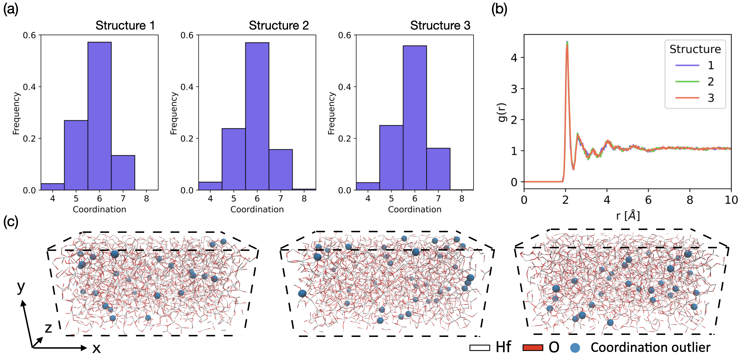
We use the example of a-HfO2 to investigate the structural differences between samples generated from different starting melt-quench processes. In Fig. 6 we plot the O-coordination of each Hf atom and the radial distribution function (where r is the inter-atomic distance) for each of the three structures. The distribution in the coordination and dispersion of the peaks in indicates the amorphous nature of the three structures. Variations between them appear as perturbations in these two quantities. We additionally plot the spatially resolved O-coordination of Hf atoms along the longest, x coordinate for the three structures, as well as the distributions of outliers (Hf atoms with very low and very high O-coordination), demonstrating a significant degree of dissimilarity among the structures.
Appendix F Near-sightedness of the Hamiltonian matrix
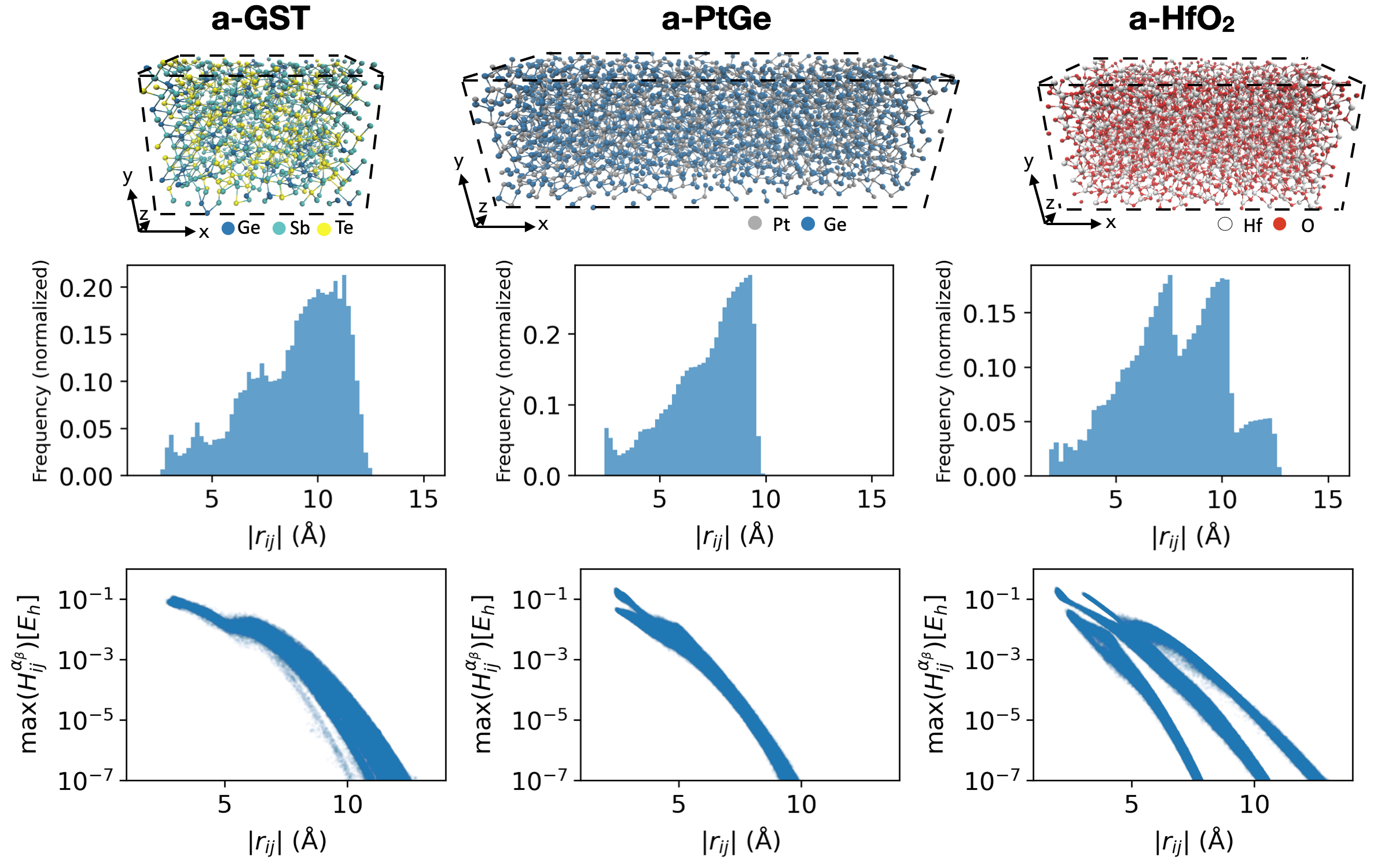
In Fig. 7, we visualize the matrix elements corresponding to the Hamiltonian of one sample of each material from the dataset. Specifically, we show the interaction ranges at which non-zero matrix elements exist, as well as their decay with increasing interatomic distance. When using a local basis, this near-sightedness holds strictly.
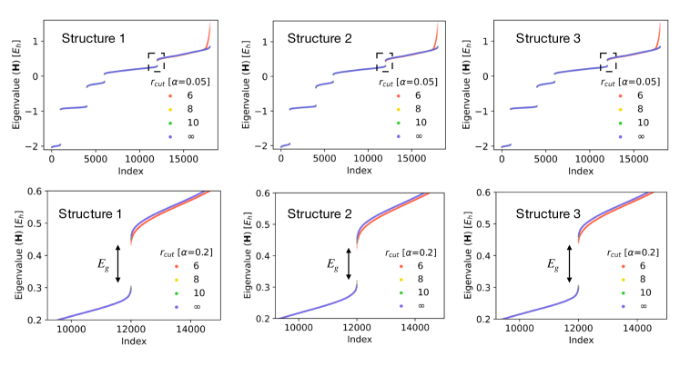
Next, using the three a-HfO2 structures in Table 1 as an example, we show the distribution of energy eigenvalues in Fig. 8 at different values of . In the second row, we zoom into the range of eigenvalues around the energy bandgap, which is defined by the transition between occupied and unoccupied electronic states (the Fermi level = in all cases). Values of 8Å create no noticeable difference on the eigenvalue spectra. Note that the value of corresponds to the case where no nonzero values were filtered from .
To demonstrate the locality of long- and short-range perturbations, we introduce a single perturbation at one chosen location in the structure and measure the mean absolute error of the onsite Hamiltonian blocks when compared to that of the unperturbed structure. The types of perturbations introduced include translation of a hafnium atom, oxygen vacancy, and substitution of an oxygen atom with a hafnium one, and are plotted against the distance from perturbation in Fig. 9 (a), (b), and (c), respectively.
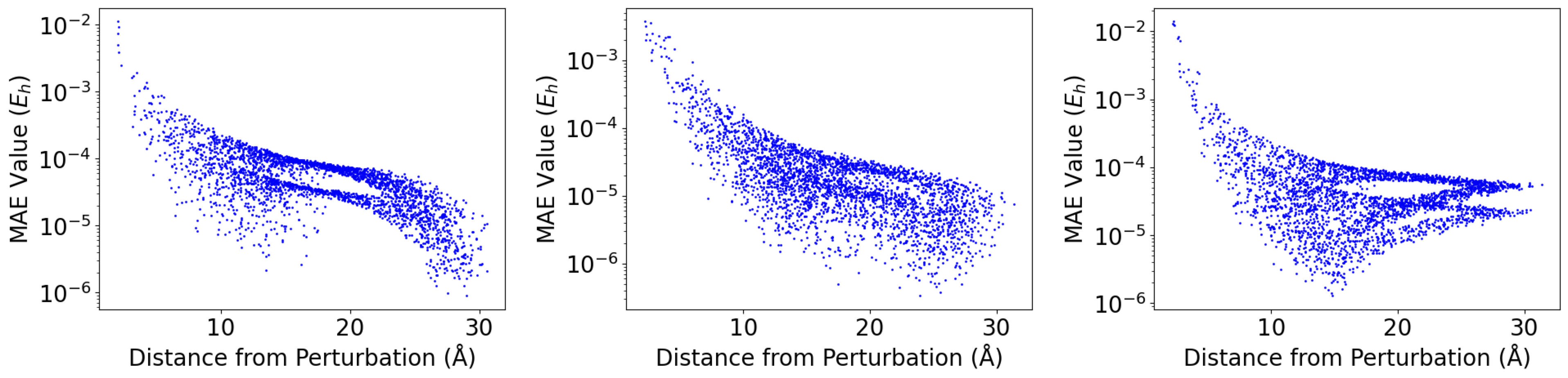
In all cases, the effect of the perturbation rapidly decays with increasing distance. For the case of the 0.1 Å translation, the average onsite MAE at a distance of 8 Å away is given by . Considering the average value of an onsite Hamiltonian block ( ), the perturbation only affects the matrix elements by 0.24% overall. Similarly, for vacancy and substitution perturbations, the matrix elements of atoms located 8 Å away only changed by 0.18% and 0.12% respectively. This implies that for our chosen cutoff of 8 Å, perturbations occurring outside of the radius surrounding the atom have a negligible effect on its Hamiltonian matrix elements. This also indicates that the electronic structure of that atom can be learned using information from the local atomic environment.
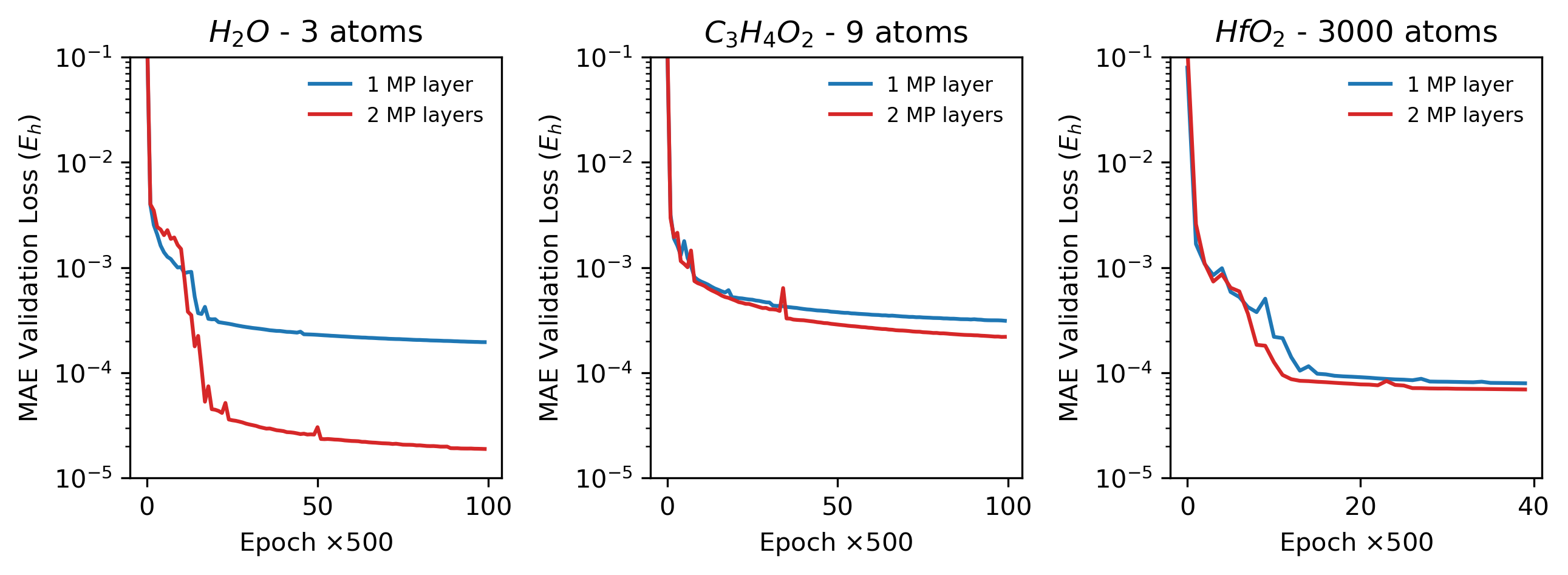
Finally, in Fig. 10 we look at the effect of using multiple Message Passing (MP) layers on the training process of HfO2, compared with that of two small molecules (H2O and C3H4O2) taken from the MD17 dataset (Christensen & lilienfeld, 2020). While the use of an additional MP layer has a significant influence on the training of H2O, this effect is reduced for the larger graphs where each atomic environment can contain richer information.
Appendix G Cutoff radius and connectivity
We now explore the minimal graph connectivity that can be used by the network to accurately learn relevant features of HfO2. To do this we use the slice partition approach introduced in Section 3.3, using a single slice of length = 3 Å to train the network. Results are reported in (Table. 7). Reducing the value of below 8 Å noticeably increases the error (), thus demonstrating the sensitivity of to the exact connectivity of the graph. Going from = 8 Å to 10 Å , the node error begins to plateau, but the node degree (which is proportional to the memory consumption of the network) grows by 1.7. This is consistent with the negligible changes to the eigenvalue spectra with of 8 Å (Fig. 8).
| [Å] | Epochs | ||||
|---|---|---|---|---|---|
| 4 | 20.99 | 10.81 | 13,816 | 4.14 | 9.60 |
| 6 | 74.23 | 27.78 | 14,071 | 3.79 | 0.40 |
| 8 | 177.09 | 51.17 | 18,245 | 3.76 | 0.22 |
| 10 | 346.03 | 81.25 | 22,463 | 3.76 | 0.15 |
We perform a similar study on the cutoff radius of PtGe in Table 8. Increasing the cutoff radius once again increases the overall prediction accuracy of the trained model, mostly due to improvements in edge-prediction accuracy.
| Cutoff [Å] | ||||
|---|---|---|---|---|
| 6 | 0.87 | 0.15 | 0.17 | 4.60 |
| 8 | 0.87 | 0.09 | 0.10 | 2.73 |
| 16 | 0.87 | 0.05 | 0.05 | 1.43 |
Appendix H Compute environment and runtime comparisons
The training is performed with PyTorch Distributed Data Parallel (Li et al., 2020), where the graph partitions (slices) can be distributed between GPUs.
H.1 Memory consumption of full-graph training
During the training of the full graph model, the peak memory consumption observed was 61.68 GiB on a single NVIDIA A100 GPU. Most of the consumption does not stem from the network and the structure but from the additional memory needed for the convolution operations.
H.2 Scalability of augmented partitioning
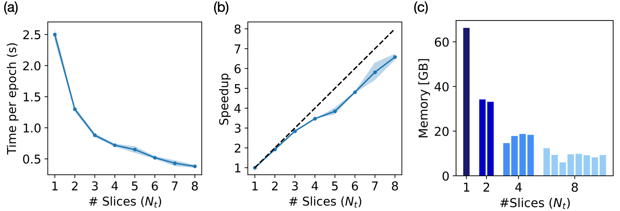
In Fig. 11, we show the decrease in time per epoch and resulting speedup when using the augmented partitioning approach introduced in Section 3.3. Since the partitions are independent, the only communication involved in every epoch is a collective to inform each GPU/rank of the loss of each other rank. The time per epoch thus decreases uniformly with the number of slices () used.
Despite the independence of each batch and the minimal communication per epoch, the scaling is not perfectly linear. The deviation from an ideal speedup can be attributed to two factors:
-
•
Load imbalance: The partitioning approach was designed to leverage the periodicity in the - and - direction within a straightforward implementation. However, it is not ideal in terms of the number of cuts/number of virtual nodes/edges required, resulting in a slightly different amount of work per rank which leads to an observable load imbalance at higher . This effect can be seen in the allocated memory per partition (Fig. 11(c)). We note that the augmented partitioning method can be used with any standard graph-partitioning algorithm.
-
•
Computational overhead of the virtual nodes and edges: Individual nodes and edges of the graph can be repeated in labeled and virtual node lists. Treating the replicas introduces additional computational cost while training the network, which increases with . This overhead is maximum with the use of very small slices (large ), thus introducing a trade-off between parallelism and time per epoch.
H.3 H2O vs HfO2 runtimes
In Section 4.5, we make a comparison between the computational cost of computing the Hamiltonian for an H2O molecule and the HfO2 structure. To approximate the cost of generating them under the same computational conditions, we set up CP2K simulations with a DZVP basis for H2O. The computation time per H2O molecule was 7s, when run on 12 nodes with 12-core Intel Xeon E5-2680 CPUs and NVIDIA P100 GPU, resulting in a total of 0.04 node hours. The HfO2 structures require 3.65 node hours in the same compute environment (but distributed to 27 nodes). The difference, omitting scaling behavior, is roughly 100.
Appendix I Additional Tests
I.1 Using two HfO2 structures for training
While training on a single structure is sufficient to achieve the results in Fig. 5, increasing the quantity of training data leads to improved prediction accuracy. To demonstrate this, we train using augmented partitioning on two structures, including structure 2 from Table 1 as well as a newly generated structure ”0” of similar size (3000 atoms). Training was performed with 18 slices of 3 Å thickness taken from both structures, validated on structure 1, and tested on structure 3. The results are compared against the previous model trained on one structure in Table 9, showing that the prediction accuracy can be improved from 5.87 to 3.55 .
| Structures | Epochs | |||||
|---|---|---|---|---|---|---|
| Training | Testing | |||||
| 0 | 3 | 15,675 | 2.29 | 0.20 | 0.22 | 5.87 |
| 0, 2 | 3 | 48,356 | 2.22 | 0.12 | 0.13 | 3.55 |
I.2 Sub-stoichiometric hafnium oxide
Here, we provide a more detailed study on the prediction of substoichiometric HfO2, where the train/test structures contain different vacancy fractions. 18 slices (tslice = 3 Å) were used in all cases. Note that for this experiment, the maximum number of epochs was fixed at 20,000. The results are summarized in Table 10. The and values across different experiments lie within a small range (2.50-2.90 and 0.16-10.18 respectively), showing that the network generalizes well to structures of different vacancies, regardless of which vacancy configuration it was trained on. To demonstrate that the augmented partitioning approach similarly does not affect accuracy for sub-stoichiometric HfOx, we also perform full graph training using structure 2 with 15% vacancies, and compare with the augmented partitioning approach in Table 12. The minimal difference in and values between full and partitioned approaches indicates that both approaches generalize equally well to different stoichiometry. These values are also close to that of stoichiometric HfO2 in Table 3.
| Stoichiometry () | |||
|---|---|---|---|
| Training | Testing | ||
| 2.44 | 0.16 | ||
| 2.58 | 0.18 | ||
| 2.50 | 0.17 | ||
| 2.48 | 0.18 | ||
| 2.50 | 0.17 | ||
| 2.60 | 0.18 | ||
| 2.94 | 0.16 | ||
| 2.52 | 0.16 | ||
| 2.52 | 0.16 | ||
I.3 Partitioning tests for other materials
For each material, we train the model on partitions of different thicknesses containing the same number of atoms. The results are summarized in Table 11.
| Material | [Å] | [Å] | |||||||
|---|---|---|---|---|---|---|---|---|---|
| a-GST | 30 | 1 | 12 | 710 | 138532 | 1.10 | 0.09 | 0.09 | 2.53 |
| a-GST | 5 | 6 | 12 | 710 | 48356 | 0.97 | 0.10 | 0.10 | 2.77 |
| a-PtGe | 50 | 1 | 8 | 1633 | 182372 | 0.81 | 0.08 | 0.09 | 2.37 |
| a-PtGe | 5 | 10 | 8 | 1633 | 84416 | 0.78 | 0.08 | 0.09 | 2.39 |
The same test was also repeated on substoichiometric HfO1.7 and tested on structures with different stoichiometry (shown in Table 12. It can be seen that augmented partitioning preserves the accuracy of prediction for all material cases studied. For HfOx, it also preserves the model’s ability to generalize to structures of different stoichiometry.
| Training method | Stoichiometry () | ||
|---|---|---|---|
| Testing set | |||
| partitioned | 1.9 | 2.94 | 0.16 |
| partitioned | 1.8 | 2.52 | 0.16 |
| partitioned | 1.7 | 2.52 | 0.16 |
| full | 1.9 | 2.96 | 0.19 |
| full | 1.8 | 2.67 | 0.18 |
| full | 1.7 | 2.64 | 0.17 |