Rapid follow-up of infant supernovae with
the Gran Telescopio de Canarias

The first few hours of a supernova contain significant information about the progenitor system. The most modern wide-field surveys that scan the sky repeatedly every few days can discover all kinds of transients in those early epochs. At such times, some progenitor footprints may be visible, elucidating critical explosion parameters and helping to distinguish between leading explosion models. A dedicated spectroscopic classification programme using the optical spectrograph OSIRIS mounted to the Gran Telescopio de Canarias was set up to try to obtain observations of supernova at those early epochs. With the time awarded, we obtained spectra for 10 SN candidates, which we present here. Half of them were thermonuclear SNe, while the other half were core-collapse SNe. Most (70%) were observed within the first six days of the estimated explosion, with two being captured within the first 48 hours. We present a characterization of the spectra, together with other public ancillary photometry from ZTF and ATLAS. This programme shows the need for an accompanying rapid-response spectroscopic programme to existing and future deep photometric wide-field surveys located at the right longitude to be able to trigger observations in a few hours after the discovery of the supernova candidate. Both the future La Silla Southern Supernova Survey (LS4) and the Legacy Survey of Space and Time (LSST) both located in Chile will be providing discovery and follow up of most of the transients in the southern hemisphere. This paper demonstrates that with a rapid spectroscopic programme and stringent triggering criteria, obtaining a sample of SN with spectra within a day of the explosion is possible.

1 Introduction

Supernovae (SNe) mark the termination of massive stars and white dwarfs (WDs), releasing as much luminous energy as the Sun produces over its entire lifetime. As cauldrons of nucleosynthesis, SNe provide the interstellar medium with heavy elements, while their enormous kinetic energy ($\sim$10⁵¹ erg) drives galaxy evolution (e.g. Hoyle & Fowler 1960; Burrows 2000). Moreover, given their high intrinsic peak luminosity, SNe serve as excellent cosmological distance indicators used to map out the expansion history of the universe (Riess et al., 1998; Perlmutter et al., 1999; de Jaeger et al., 2020).

Beside direct progenitor detections in archival images, and nebular spectra, much of what we know about SNe and their progenitors is based on observations of objects obtained a few days/weeks after the explosion. These SNe were discovered by searches that repeatedly observed a number of targeted galaxies (e.g. the Lick Observatory Supernova Search, LOSS, Filippenko et al. 2001; the CHilean Automatic Supernova sEarch, CHASE, Pignata et al. 2009) or by search programs that repeatedly scanned large sections of the sky (e.g., the Sloan Digital Sky Survey II - SN Survey, SDSS-II/SN, Frieman et al. 2008; the Palomar Transient Factory, PTF, Rau et al. 2009; the Nearby SN Factory, Aldering et al. 2002) combined with other dedicated follow-up programmes to obtain dense, multiwavelength observations of nearby SNe (e.g. the Carnegie Supernova Project, CSP, Krisciunas et al. 2017; Phillips et al. 2019; the Center for Astrophysics SN programme, CfA, Hicken et al. 2009, 2012).

More recently, to expand our understanding of the various SN types and the physics of their explosions and progenitor systems, wide-field untargeted surveys such as the All-Sky Automated Survey for Supernovae (ASAS-SN; Shappee et al. 2014), the Asteroid Terrestrial Impact Last Alert System (ATLAS; Tonry et al. 2018; Smith et al. 2020a), the Panoramic Survey Telescope and Rapid Response System (Pan- STARRS; Chambers et al. 2016), and the Zwicky Transient Facility (ZTF; Bellm et al. 2019; Graham et al. 2019), are regularly obtaining high-cadence, in some cases intra-day, observations and discovering SNe and other transients in hours to days after the explosion. This dense cadence has led to the discovery of a multitude of new types of transient phenomena (e.g., SuperLuminous SN, fast-and-faint transients, & relativistic transients), revealed a population of transients at all luminosity scales, and yielded less biased results compared to previous targeted surveys.

Table 1: SNe Properties.

Name	IAU Name	Type	R.A.	Dec	Host Galaxy	E(B-V) MW (mag)	tobs-t${}_{lnd}^{\rm reported}$	tobs-tdisc	TNS Report
ZTF20aaxvzja	2020itj	IIb	14:34:48.394	+08:10:10.42	CGCG 047-108	0.0211$\pm$0.0006	16h39.94m	15h05.84m	[1]
ZTF20aaynrrh	2020jfo	II	12:21:50.480	+04:28:54.05	M61	0.0194$\pm$0.0001	4d15h06.93m	16h51.43m	[2]
ATLAS20lti	2020jgl	Ia	09:28:58.426	$-$14:48:19.88	MCG -02-24-027	0.0585$\pm$0.0016	1d14h12.80m	14h34.39m	[3]
ATLAS20lts	2020jhf	Ia	13:14:53.440	+27:00:31.10	UGC 8325	0.0103$\pm$0.0006	3d12h07.48m	1d11h48.75m	[4]
ZTF20abaovyz	2020kjt	II	18:43:16.457	+71:40:36.60	WISEA J184316.29+714032.6	0.0462$\pm$0.0011	1d16h07.03m	18h58.49m	[5]
ZTF20abapyxl	2020kku	Ia	17:32:33.723	+15:44:09.17	WISEA J173233.56+154410.2	0.0909$\pm$0.0017	20h02.58m	18h28.06m	[5]
ZTF20abbhyxu	2020kyx	Ia	16:13:45.510	+22:55:14.38	CGCG 137-064	0.0768$\pm$0.0029	1d21h57.10m	22h02.15m	[6]
ZTF20abbplei	2020lao	Ic-BL	17:06:54.600	+30:16:17.40	CGCG 169-041	0.0432$\pm$0.0010	21h07.81m	18h45.72m	[7]
ZTF20abisitz	2020nny	II	22:58:34.228	+15:10:15.07	IC 1461	0.0384$\pm$0.0006	1d20h26.74m	17h12.89m	[8]
ZTF20abtctgr	2020rlj	Ia-91bg	23:01:09.614	+23:29:14.00	WISEA J230109.61+232903.7	0.1098$\pm$0.0036	1d20h59.64m	21h55.85m	[9]

It is through early-phase observations that we can estimate critical explosion parameters (previously out of reach with traditional studies), delineate between leading explosion models, and study the local environment of cosmic explosions (e.g., Fraser et al. 2021; Ashall et al. 2022). In particular for SNe, this corresponds to the epochs when the photosphere is close to the outer layers of the exploding progenitor, uncovering more insights about its nature. In the literature, there has been a lack of SN early-epoch spectra given the difficulty of discovering transients right after explosion, but this is now changing.

With this in mind, we started a spectroscopic programme at the 10.1 m Gran Telescopio de Canarias (GTC) to obtain early spectra of SN candidates within 48 h of the explosion that complements imaging surveys. These observations would probe the outermost layers of the ejecta, helping to distinguish between explosion and progenitor scenarios and to answer questions such as the origin of the bimodality in the early phase $(B-V)$ colors of SNe Ia (Stritzinger et al., 2018), the pre-SN masses of the progenitors of stripped-envelope core-collapsed SNe (Stritzinger et al., 2020), and the outermost structure and environment of the red giant progenitors of Type II SNe (Förster et al., 2018). This early-time spectroscopy, benefiting from the large aperture of GTC, has the potential to offer new insights into the composition of the outer layers of SN progenitors right before the explosion, as well as yield new clues regarding the underlying physics of different types of supernovae.

Additionally, a parallel goal of the programme was to find type Ia supernovae (SNe Ia) to feed potential candidates for the Supernovae in the near-InfraRed Avec Hubble (SIRAH; Jha et al. 2020; Galbany 2020), a Hubble Space Telescope (HST) Cycle 27+28 and NOAO/Gemini programme to obtain NIR HST spectra of a sample of 24 Hubble-flow ($0.02<z<0.07$) target-of-opportunity SN Ia, supplemented by the Gemini NIRI and FLAMINGOS2 imaging data to obtain the full NIR light curves. The main goals of SIRAH are to (i) build NIR spectrophotometric templates that will serve as a foundation for the Nancy Roman Space Telescope SN survey (Rose et al., 2021); (ii) yield NIR-only SN Ia measurement of the Hubble constant ($H_{0}$); and (iii) constrain dark energy together with data from the RAISINs surveys (Jones et al., 2022), producing a NIR Hubble diagram from $z=0.02$ to $z=0.6$ all calibrated on the WFC3/IR photometric system. Once a SN candidate is classified and identified as an early SN Ia, an HST trigger is sent with enough anticipation that a spectrum, which typically requires one to two weeks for execution, is obtained around the epoch of maximum brightness. Under our GTC programme, we contributed two SNe Ia to SIRAH (SNe 2020jgl and 2020kyx). Their ZTF and ATLAS light curves and spectra are presented here.

The paper is organized as follows: in Section §2, we describe the strategy followed to select our targets. In Section §3, we explain the GTC data reduction and how we collected publicly available multi-band optical light curves. In Section §4, we analyze the collected data by determining the SN spectral typing, estimating the time of first light and the maximum brightness epochs, characterizing their light-curves, determining the GTC spectra epoch, and measuring SN photospheric velocities. In Section §5, we perform a more detailed analysis on two well-observed SNe, for which more follow-up data have been obtained: the type IIb SN 2020itj and the type Ia SN 2020jgl. Finally, in Section §6, we summarize our work and discuss improvements for future similar early SN programmes.

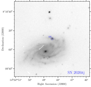
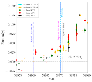
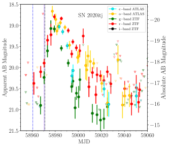
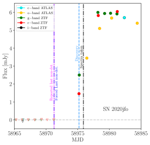
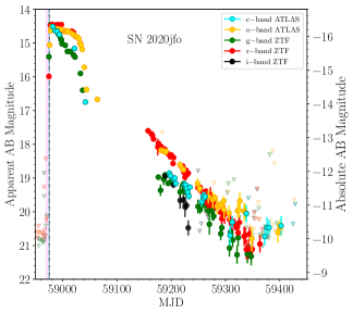
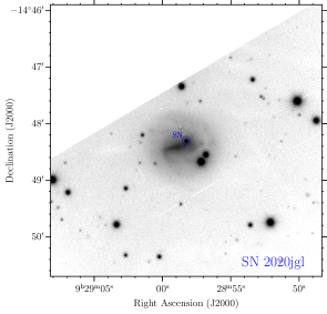
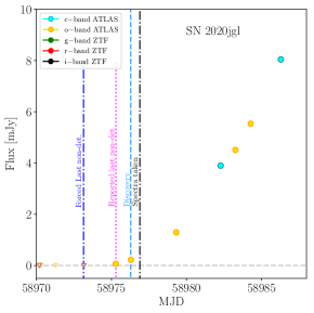
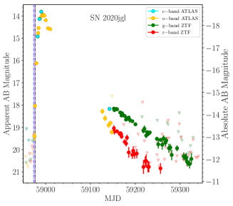
Figure 1: SN finder and combined light curves in the observer’s frame. Left panel: Host-galaxies images for our SNe sample. The SNe are marked with blue circles. Middle panel: Early-time light curve of our SNe sample in flux units. The circles represent detections whereas the triangles are considered non-detections. Vertical lines denote the last non-detection from forced photometry (dashed-dotted blue), the reported last non-detections at the time of discovery (dotted magenta), the time of discovery (dashed clear blue), and the time when each spectrum was taken with GTC/OSIRIS (dashed-dotted black). Right panel: SN light curves in magnitude space (apparent magnitude marked in the left y-axis and the absolute magnitude in the right y-axis; see Section 3.3 for information on distances). Downward-facing triangles denote 3$\sigma$ upper limits.

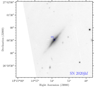
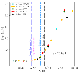
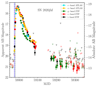
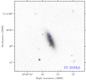
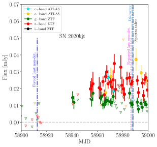
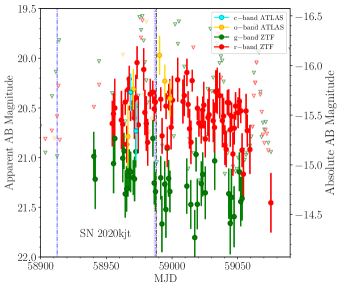
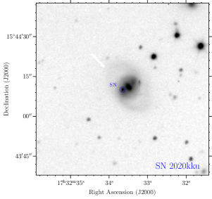
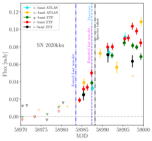
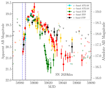
Figure 2: (cont.)

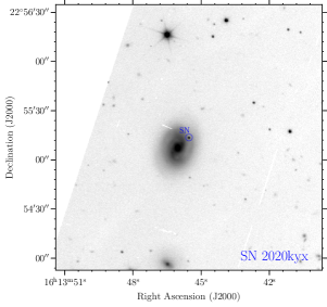
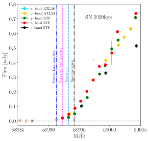
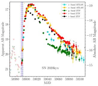
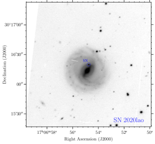
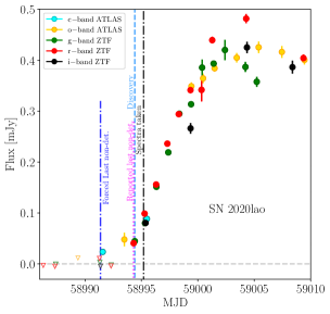
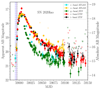
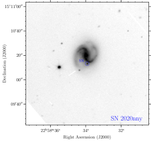
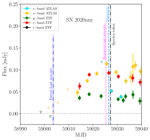
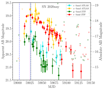
Figure 3: (cont.)

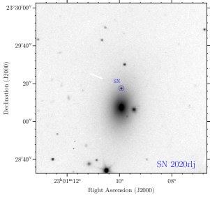
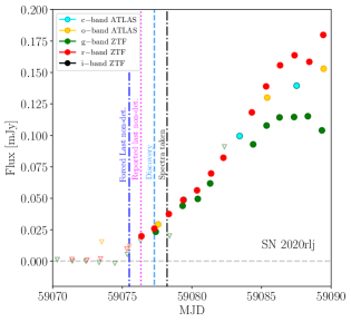
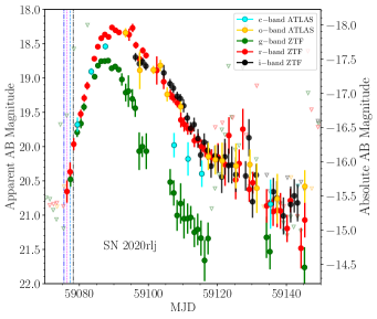
Figure 4: (cont.)

2 Strategy

Our programme ran intermittently from May to August 2020. The baseline approach we followed to select our candidates was using The Automatic Learning for the Rapid Classification of Events (ALeRCE) Alert Broker (Förster et al., 2021) through its Supernova Hunter tool. Every day, right after observations by ZTF at the Palomar observatory were finished (about 11h UT in May 2020; 13h local CET), we checked the ALeRCE SN Hunter for new SN candidates. Usually, about a hundred objects pass the criteria to be considered reliable SN candidates. They were visually checked to select those that fulfill two criteria: (i) There was a ZTF difference-imaging non-detection of the candidate from the previous night, so the object had a high probability of having exploded in less than 24 hours, and (ii) it was clearly associated with a spatially resolved host galaxy, so the host galaxy redshift could be used to determine the absolute magnitude of the SN and check whether it was consistent with a typical young SN brightness. Only in a couple of cases (SN 2020jgl and SN 2020jhf), when ZTF did not provide candidates, and the ALeRCE SN Hunter list was empty, we directly checked for newly reported SN candidate discoveries at the Transient Name Server (TNS) page. ATLAS reported these new objects. Also, in a couple of cases (SNe 2020jfo and 2020jhf), we did not follow criterion (i), and we triggered observations anyway, given the faint reported discovery magnitude. As we will show in Section 4, they ended up being early spectra.

Most days, there were no objects that fulfilled both criteria. But when a good candidate appeared, we immediately triggered optical spectroscopy with the Optical System for Imaging and low-Intermediate-Resolution Integrated Spectroscopy (OSIRIS) at the 10.1m Gran Telescopio de Canarias (GTC) using our ToO programme Follow-up of infant supernovae within 48h from explosion (GTC52-20A). For that, the phase 2 form was filled in with the ALeRCE finding chart, the SN candidate coordinates and exposure times that varied from 500 to 900 sec in each of the two grisms used (R1000B and R1000R).

Observations were typically executed the same night, ensuring less than 24 hours had passed since discovery. There is one exception, SN 2020jhf, that could not be observed on the same night of the trigger due to weather conditions, and it was observed the following night, $\sim$35 hours after discovery. In total, we triggered 10 times. Table 1 summarizes the information of the 10 SNe observed under the programme and presented here: ZTF/ATLAS and IAU names; SN type (see Section 4.1); coordinates; host galaxy name; Milky Way line-of-sight reddening $E(B-V)$ obtained from IRSA Galactic Dust Reddening and Extinction map (Schlafly & Finkbeiner, 2011); the time between the spectroscopic observation and the reported last non-detection, $t_{\rm obs}-t_{\rm lnd}$; the time between the spectroscopic observation and the discovery epoch, $t_{\rm obs}-t_{\rm disc}$; and the respective astronote reference, since all classifications were publicly reported in TNS. Table 16 summarizes additional observational information.

Three SNe (SNe 2020itj, 2020kku, and 2020lao) had intra-night initially reported non-detections. As described in section 3.3, these reported non-detections resulted in detections a posteriori using forced photometry. The left column of Figure 1 shows the SN location in their host galaxy from OSIRIS acquisition images.

3 Data

The long-slit spectroscopic observations of our sample were taken with the OSIRIS instrument mounted in the GTC 10.1m telescope at the Roque de los Muchachos Observatory in the Canary Islands. Observations were conducted using the R1000B and R1000R grisms with contiguous wavelength ranges 3630-7500 Å and 5100-10000 Å and a dispersion of 2.12-2.62Å/pix, respectively, and a spectral resolution of about 1100.

In this section, we summarize the reduction process for the spectroscopic data and introduce the public photometric measurements retrieved from the Zwicky Transient Facility (ZTF) and Asteroid Terrestrial-impact Last Alert System (ATLAS) surveys that will be used in the following analysis.

3.1 Data Reduction

We conducted the reduction process utilizing a Python-based pipeline developed by our team, which utilizes version 1.11.0 of PypeIt (Prochaska et al., 2020a, b). PypeIt is a python package designed to reduce spectroscopic data from several different spectrographs. The pipeline performed the following reduction steps: bias subtraction, flat-field correction, wavelength calibration (using HgAr, Ne, and Xe arc lamps as reference), sky subtraction, and flux calibration. For the telluric correction, we assessed the H₂O and O₂ telluric absorption features from the standard star’s spectrum obtained on the same night of each SN observation. A spectrum equal to the unity was created except on the wavelength ranges of the telluric absorption features mentioned previously. By dividing the SN spectrum by this transmission spectrum, we obtained each SN’s final one-dimensional telluric-corrected flux-calibrated spectrum.

Table 2: Redshifts obtained from the spectral lines coming from the galaxy hosts.

IAU Name	$\lambda_{\text{observed}}$ (Å)							z${}_{\text{host}}$		$\mu$ (mag)
	H$\beta$	[O III]	[O III]	Na I D	H$\alpha$	[S II]	[S II]	SN spec	Host spec
2020itj	5022.66	5123.75	5172.99	$-$	6780.16	6938.99	6954.41	0.0332$\pm$0.0001	0.03295a	35.802
2020jfo	$-$	$-$	$-$	5923.83	6598.36	$-$	$-$	0.0053$\pm$0.0001	0.00522b	30.810$\pm$0.200
2020jgl	$-$	$-$	$-$	$-$	$-$	$-$	$-$	$-$	0.00676b	32.428$\pm$0.089
2020jhf	$-$	$-$	$-$	5985.92	6664.92	$-$	$-$	0.0157$\pm$0.0001	0.01544a	34.127
2020kjt	5040.27	$-$	5191.70	$-$	6808.13	6967.42	6982.07	0.0372$\pm$0.0002	$-$	36.072
2020kku	$-$	$-$	$-$	6385.03	$-$	$-$	$-$	0.0835$\pm$0.0004	0.08356c	37.901
2020kyx	$-$	$-$	$-$	$-$	$-$	$-$	$-$	$-$	0.03192a	35.731
2020lao	$-$	$-$	$-$	$-$	6764.89	6924.02	6939.43	0.0309$\pm$0.0001	0.03081a	35.653
2020nny	5010.28	$-$	$-$	6074.94	6765.18	6922.74	6937.57	0.0308$\pm$0.0001	0.03084a	35.655
2020rlj	$-$	$-$	$-$	$-$	$-$	$-$	$-$	$-$	0.03976b	36.221

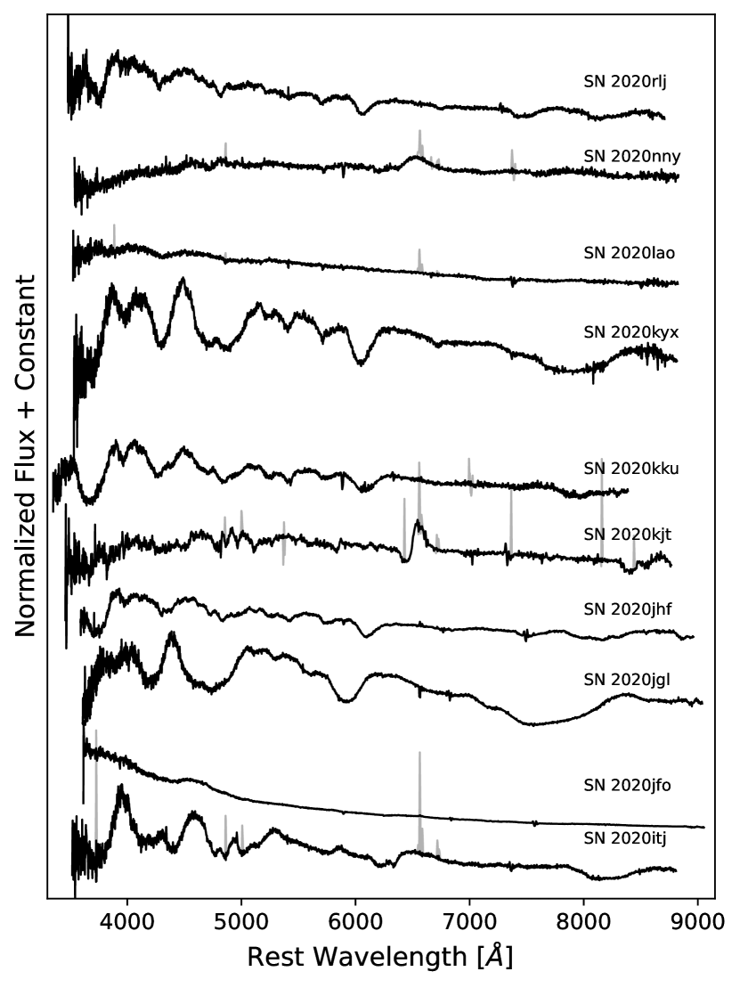
Figure 5: GTC/OSIRIS spectra of the 10 SNe in our dataset. Each spectrum has been corrected for Milky Way reddening and redshift and thus is on the rest wavelength frame. The spectra were cleaned for narrow emission lines from the host galaxy and some spikes due to cosmic rays. Each spectrum was normalized by the flux average in the wavelength range 4500-5000 Å and added an arbitrary constant for clarity.

3.2 Redshift and distance

We estimated the redshift of each SN by measuring the host galaxy’s narrow spectral lines present in the SN spectra. The following lines were considered: Balmer H$\alpha$ and H$\beta$ at 6562.81 and 4861.35 Å, respectively, [O III] doublet at 4958.911 Å and 5006.843 Å, Na I D at 5893 Å and [S II] doublet at 6716.44 and 6730.82 Å. All of these spectral features are in emission except for Na I D, which is in absorption. We used IRAF (Image Reduction and Analysis Facility, Tody 1986) to fit a Gaussian profile to the lines and estimate their center in wavelength. Then, we computed the redshift values considering the shift of each line from its rest-frame wavelength. The final redshift value and respective uncertainty were taken as the mean of the different values and the standard deviation, respectively. For the case of SN 2020kku, we only measured the Na I D absorption line, thus we took the wavelength step as a conservative estimate of the uncertainty associated with the final redshift value, which we then obtained through error propagation.

Table 7 shows the central wavelengths of the lines detected in each SN along with the final computed redshift. SNe 2020jgl, 2020kyx, and 2020rlj lacked spectral lines from their respective galaxy hosts. Along with the redshift values estimated in this work, Table 7 shows public spectroscopic redshift measurements of the respective hosts. The redshifts estimated from the SN spectra include the contribution of the galaxy’s rotational velocity, thus the final redshift values that we adopt throughout this work are the ones coming from the galaxy’s spectra. The only exception is SN 2020kjt, where no public spectroscopic redshift was found.

We determined the distance modulus of the SN host galaxies assuming a flat-$\Lambda$CDM model with H${}_{0}=70$ km s^-1 Mpc^-1 and $\Omega_{m,0}=0.3$ and using the redshift measured above for all SNe, except for SN 2020jfo and SN 2020jgl. For these former two SNe, we obtained redshift-independent based distances from the NASA/IPAC Extragalactic Database (NED) since they are very nearby, and the contribution of peculiar velocities may be significant when using cosmological redshifts. SN 2020jfo exploded in the spiral galaxy M61, which is at a redshift $z=0.005224$ according to NED. There are several distance measurements for this nearby host. In this work, we assume the distance 14.51$\pm$1.38 Mpc ($\mu=30.81\pm 0.20$ mag) obtained in Bose & Kumar (2014) considering redshift-independent methods based on optical data of SN 2008in. Sollerman et al. (2021), Ailawadhi et al. (2023) and Kilpatrick et al. (2023) also assume the same distance value whereas Teja et al. (2022) finds a distance of 16.45$\pm$2.69 Mpc ($\mu$ = 31.08$\pm$0.36 mag), which is in agreement with the value found here within the uncertainties. The host of SN 2020jgl is the face-on spiral galaxy MCG -02-24-027 located at a redshift $z=0.006758$ (NED). No distance measurements were available in the literature; thus, we obtained the distance modulus, $\mu=$ 32.428$\pm$0.089 mag, from fitting SNooPy (Burns et al., 2011) to the SN light-curve (See section 4.3).

For clarity, we masked the host galaxy contamination lines from the spectra for the following analysis. The final reduced and corrected spectra of all 10 SNe are presented in Figure 5.

3.3 Light curves

We obtained forced photometry of the 10 SNe in our sample from both the ATLAS (Tonry et al., 2018; Smith et al., 2020b) survey in the orange (o, 5600 to 8200 Å) and cyan (c, 4200 to 6500 Å) bands and from the ZTF (Masci et al., 2018) survey in the g (3676 to $\sim$5614 Å), r (5498 to $\sim$7394 Å) and i (6871 to $\sim 8965$ Å) bands.

ATLAS consists of four telescopes, which automatically scan the sky several times every night, resulting in several photometric measurements. ZTF can also have several data points on each band per night. Aiming to obtain a clearer perception of the light curves’ behaviour, we performed a binning on the photometric data. Thus, the forced photometry flux measurements and uncertainties retrieved on the same night, using the same band, were combined as the weighted average and the mean deviation, respectively. Then, we produced the light curves in magnitude space following the steps described in the ATLAS and ZTF documentation. We converted flux counts into flux density units (AB magnitude system) as follows,

$$f_{AB} = f_{counts}*10^{-0.4(ZP-ZP_{AB})},$$ (1)

$$\sigma_{f_{AB}} = |10^{-0.4(ZP-ZP_{AB})}*\sigma_{f_{counts}}|,$$ (2)

where $f_{counts}$ and $\sigma_{f_{counts}}$ are the flux and its respective uncertainty in count units, $ZP$ is the survey zero-point, and to ensure the flux in Janskys (Jy) units, $ZP_{AB}=8.90$. We then compute the AB magnitude and their respective uncertainties in the following way,

$$m_{det} = -2.5\times log_{10}f+ZP_{AB},$$ (3)

$$\sigma_{m} = 1.0857\frac{\sigma_{f}}{f},$$ (4)

where $f$ is the flux in Jy and $\sigma_{f}$ the flux error. We used the distance modulus presented in Table 7 to convert observed apparent magnitudes into absolute magnitudes.

Observations with a signal-to-noise (S/N) ratio higher or equal to 3 were considered as detections; otherwise, they were considered non-detections and reported as 3$\sigma$ upper limit magnitudes as,

$$m_{ndet}=-2.5\times log_{10}\left(3\sigma_{f}\right)+ZP_{AB}.$$ (5)

Therefore, we define the last non-detection as the data point immediately preceding the first detection with a deeper magnitude. Table 3 (second and third column, respectively) presents the forced photometry last non-detection and first detection estimated for our sample.

Table 3: Summary of the last-non detections, first detections, times of first light and spectra epochs.

IAU Name	Reported	Forced	Forced	Time of first light		Spectrum Date	Spectrum Epoch
	last non-detection	last non-detection	first detection	Mid-point	Early LC Fitting		Mid-point	Early LC Fitting
2020itj	58970.29	58960.50	58961.90	58961.20 $\pm$ 0.70	$-$	58971.00 $\pm$ 0.01	9.49 $\pm$ 0.68	$-$
2020jfo	58971.28	58971.28	58975.20	58973.24 $\pm$ 1.96	58974.72 $\pm$ 0.19	58975.92 $\pm$ 0.01	2.66 $\pm$ 1.95	1.18 $\pm$ 0.19
2020jgl	58975.30	58973.15	58975.30	58974.23 $\pm$ 1.08	58974.31 $\pm$ 1.14	58976.91 $\pm$ 0.01	2.66 $\pm$ 1.07	2.57 $\pm$ 1.13
2020jhf	58975.41	58974.25	58975.41	58974.83 $\pm$ 0.58	58974.76 $\pm$ 0.20	58978.93 $\pm$ 0.01	4.03 $\pm$ 0.57	4.10 $\pm$ 0.20
2020kjt	58986.47	58912.50	58940.50	58926.50 $\pm$14.00	$-$	58988.15 $\pm$ 0.01	59.44 $\pm$ 13.50	$-$
2020kku	58987.34	58983.50	58984.40	58983.95 $\pm$ 0.45	58981.81 $\pm$ 0.86	58988.18 $\pm$ 0.01	3.90 $\pm$ 0.42	5.87 $\pm$ 0.79
2020kyx	58992.27	58991.30	58992.27	58991.79 $\pm$ 0.49	58990.71 $\pm$ 0.33	58994.20 $\pm$ 0.01	2.33 $\pm$ 0.47	3.37 $\pm$ 0.32
2020lao	58994.31	58991.37	58991.58	58991.48 $\pm$ 0.11	58993.14 $\pm$ 0.18	58995.21 $\pm$ 0.01	3.62 $\pm$ 0.11	2.00 $\pm$ 0.17
2020nny	59025.34	59003.57	59013.60	59008.59 $\pm$ 5.02	59009.94 $\pm$ 0.95	59027.20 $\pm$ 0.01	18.05 $\pm$ 4.87	16.73 $\pm$ 0.92
2020rlj	59076.34	59075.50	59076.34	59075.92 $\pm$ 0.42	59074.31 $\pm$ 0.41	59078.23 $\pm$ 0.01	2.22 $\pm$ 0.40	3.76 $\pm$ 0.39

• NOTES: Numbers in bold face indicate the final time of first light. Numbers in italics indicate cases where the early light-curve method provides an estimate earlier than the forced last non-detection. This occurs because the image was not deep enough to properly detect the SN, but the early fit is considered reliable.

The resulting light curves in flux (middle panel) and magnitude (right panel) space are presented in Figure 1, along their respective finding charts (left panel). As seen in the middle panel, the reported last non-detection resulted in most cases being an actual detection in forced photometry. The only exception is SN 2020jfo, in which both estimations coincide. Generally, the last non-detection was found a few days earlier. The median for this difference is 3.5 days. However, there are some cases where the difference is larger. The most extreme case is SN 2020kjt, which has a difference of $\sim 74$ days. This is followed by SN 2020nny ($\sim 22$ days) and SN 2020jfo ($\sim 11$ days).

Given SN 2020kjt’s apparent faintness, its analysis is complicated. Thus, the last non-detection is hard to define because none of the upper limits are deeper than the actual first detection. However, our estimated non-detection seems to be accurate, considering the spectrum phase obtained from the spectral matching (section 4.4). In this object, the first detection from the forced photometry also appears many days before the reported discovery date ($\sim 50$ days earlier). Therefore, the spectrum obtained from our programme turns out to be very old ($\sim 50-70$ days from the explosion).

4 Analysis

4.1 Typing

To determine the supernova type and its epoch, we used the Supernova Identification code (SNID, Blondin & Tonry 2011) as it performs a cross-correlation to spectra in a database including thousands of observed supernova spectra of different types and at different epochs. Figure 6 summarizes a few of the best template fits obtained for each SN in our sample. Below, we comment on the different spectral matchings considering the light curves (Figure 1) and the redshift of each SNe (Table 7).

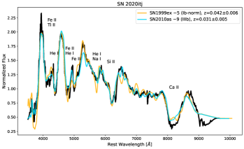
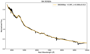
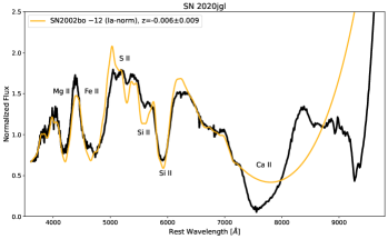
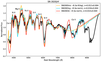
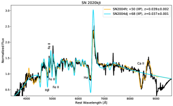
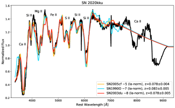
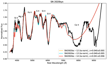
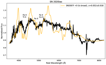
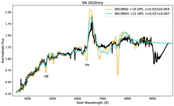
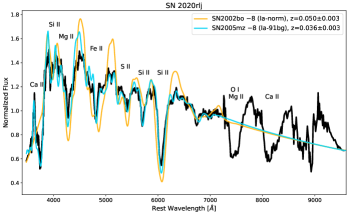
Figure 6: Best spectral template matches from SNID for each of the 10 SNe in our sample. Each fit label includes the SN name compared, the epoch from the time of maximum, the type, and the redshift. Common spectral features of each supernova type are represented in the different plots.

• SN 2020itj resembles type Ib SN 1999ex and type IIb SN 2010as at 5 and 9 days before reaching maximum brightness, respectively. With a measured redshift of 0.033, the redshift fit of SN 2010as (0.031) aligns more closely than that of SN 1999ex (0.042). Upon visual examination of the early-time light curve of SN 2020itj, both best fits offer a reliable estimate of the epoch, as it seems that the SN 2020itj spectrum was obtained about 10 days before the peak.

• SN 2020jfo exhibits the closest match with type II SN 2006bp approximately 6 days before reaching maximum brightness. The redshift of the comparison aligns well, within the margin of error, with the redshift estimated for SN 2020jfo (0.006 and 0.00522, respectively), and the epoch also appears to align well with the information obtained from the light curve.

• SN 2020jgl has a good match with the normal type Ia SN 2002bo, 12 days before maximum at redshift $\sim$0.006. However, there are not many earlier than -12 days spectra in the SNID available database, so, as we will show later (section 5.2), this spectrum could be even earlier. The estimated redshift is also in line with that found by SNID.

• SN2020jhf has as best matches to type Ia 91bg-like SN 2005mz, type Ia SN 2003cg, and type Ia SN 2003U at about 8-9 days before maximum. There is no clearly favorable fit, although we’ll show later on (section 4.3) that this SN may be a transitional from normal to subluminous (e.g. visible secondary peak, not-so-low light-curve stretch).

• SN2020kjt is best matched to type II SNe 2004fc and 2004dj at 50 and 68 from explosion, respectively. Both fits are similarly good, with SN 2004fc probably being a bit better, and consistent with a SN II in the middle of the plateau phase.

• SN2020kku is best matched with type Ia SNe 2005cf, 1990O, and 2003du at 5, 7, and 8 days before maximum, all similarly providing a reasonable fit to a normal SN Ia about a week before maximum light.

• SN2020kyx is best matched with SN2002bo at different epochs: 12, 13, and 14 days before maximum. The three spectra of SN 2002bo do not change considerably and are typical of an early spectrum two weeks before maximum normal SN Ia.

• SN 2020lao does not have a good match with any template present in the SNID database, but we overplotted the spectrum of type Ic broad-line SN 2007I at maximum light. While the fit does not perfectly match, it has similar features at similar wavelengths as SN 2020lao. We will present in a separate paper a detailed analysis of this SN, confirming it is effectively a broad-line type Ic SN (Stritzinger et al. in prep.).

• The best SNID fits for SN 2020nny are SNe II 1990E and SN 1992H at 19 and 12 days after maximum, respectively. The main feature of the spectrum, a broad H$\alpha$ emission, aligns well with that of SN 2020nny and corresponds to a similar epoch and redshift.

• SN 2020rlj has as best matches normal type Ia SN 2002bo and 1991bg-like type Ia SN 2005mz, both 8 days before their respective time of maxmimum. The 1991bg-like spectrum provides a better match, and both the redshift and the epoch matches that of SN 2020rlj.

In summary, we conclude that the dataset collected under our programme and presented in this work is composed of 5 SNe Ia (SN 2020jgl, SN 2020jhf, SN 2020kku, SN 2020kyx and SN 2020rlj), 1 SN IIb (SN 2020itj), 1 SN Ic-BL (SN 2020lao) and 3 SNe II (SN 2020jfo, SN 2020kjt and SN 2020nny).

4.2 Epoch of the first light

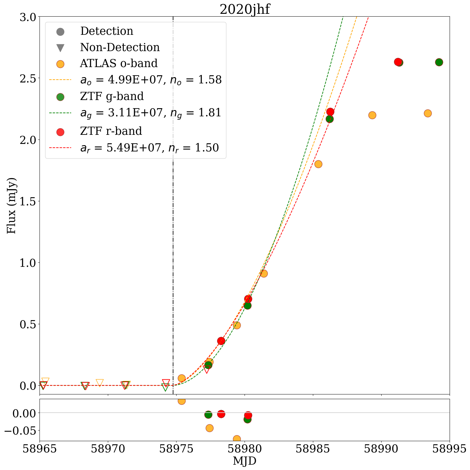
Figure 7: Early observer-frame light curve of SN 2020jhf fitted to different power laws considering each band. The black line denotes the estimated time of first light, $t_{0}=58974.76$. The estimated coefficients $a$, and $n$ from Equation 6 are shown in the legend. The ATLAS c-band did not have sufficient data points to fit a curve. The bottom panel exhibits the residuals in the fitting range, where the dotted grey line is the fit for each band.

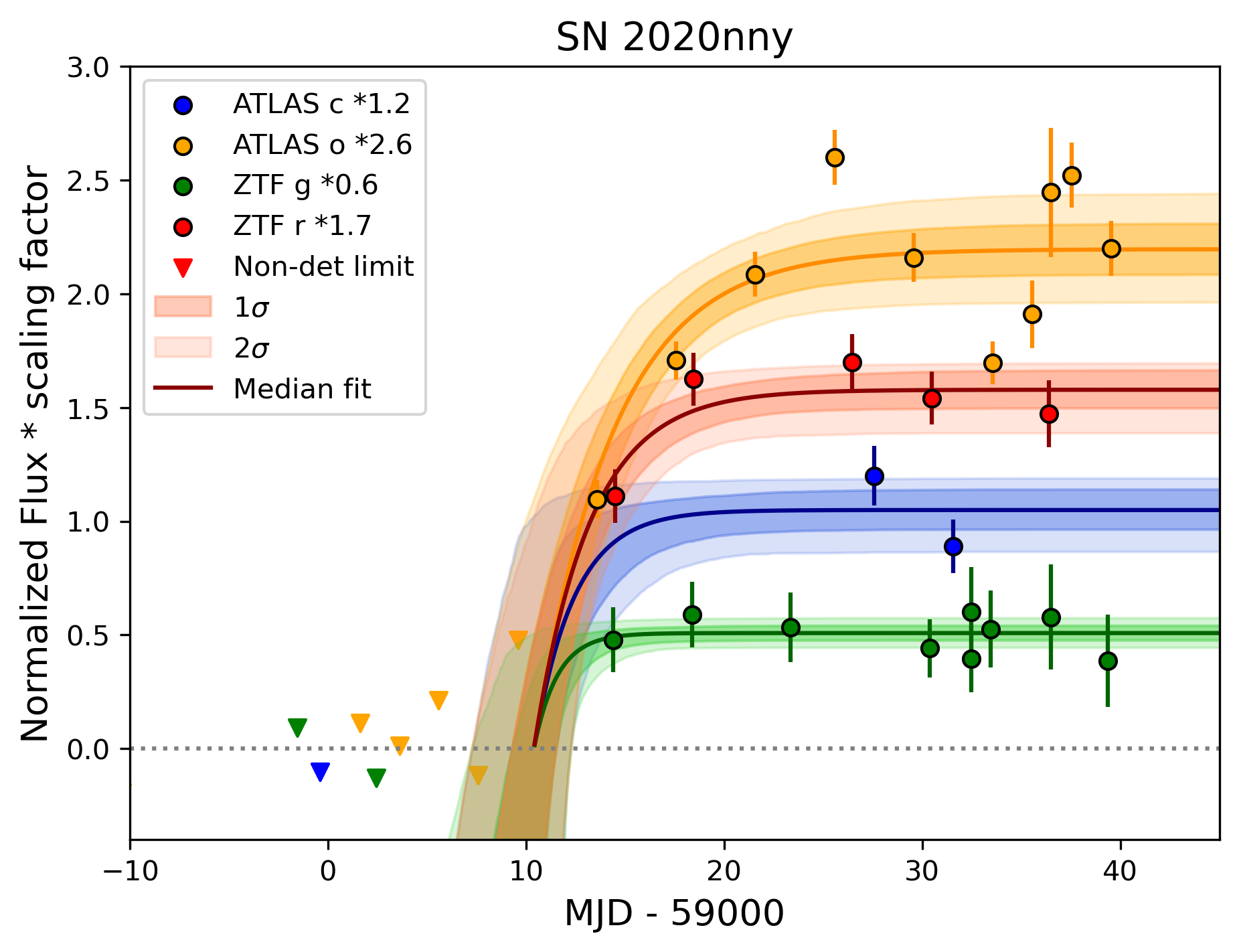
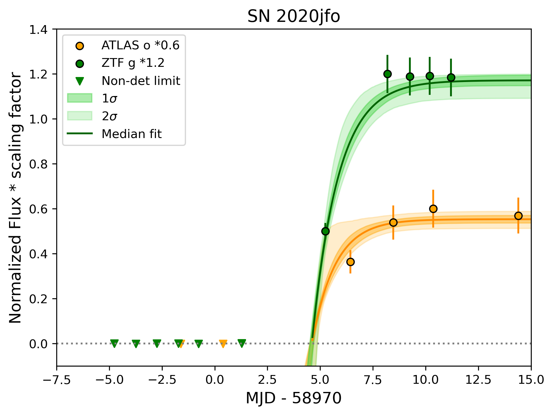
Figure 8: Inverse exponential fit on the early observer-frame light-curves of SN 2020nny (top) and SN 2020jfo (bottom). The dark solid lines show the mean fit and the shaded regions denote the 1$\sigma$ and 2$\sigma$ error regions. The flux values in the different bands were normalized and then rescaled for better clarity.

We implemented two different methods to estimate the epoch of the first light for the SNe in our dataset. The first is to compute the mid-point between the epoch of the last non-detection and the epoch of the first detection (e.g., Gutiérrez et al. 2017). The uncertainty associated with this value is equal to (MJD${}_{\rm 1st\leavevmode\nobreak\ det}-$MJD_non-det)/2. However, the accuracy of this method strongly depends on the cadence of the observations.

To try to constrain the epoch of first light better, we implement a second method, which is to fit the early rise of the light curves. For SNe type Ia and for SN 2020lao (type Ic), we fit a power law to all bands simultaneously, considering the measurements from the last non-detection up to half of the maximum flux and their respective flux uncertainties (González-Gaitán et al., 2015a),

$$f(t)=\begin{cases}\alpha\left(t-t_{0}\right)^{n},&t>t_{0}\\ 0,&t<t_{0},\end{cases}$$ (6)

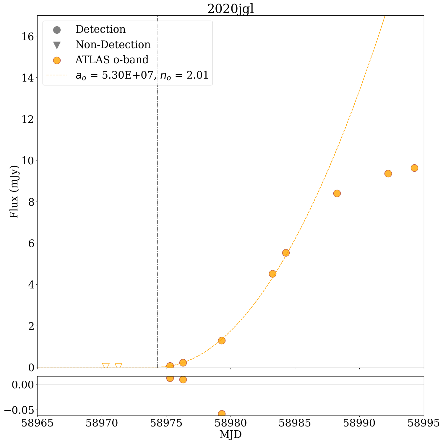
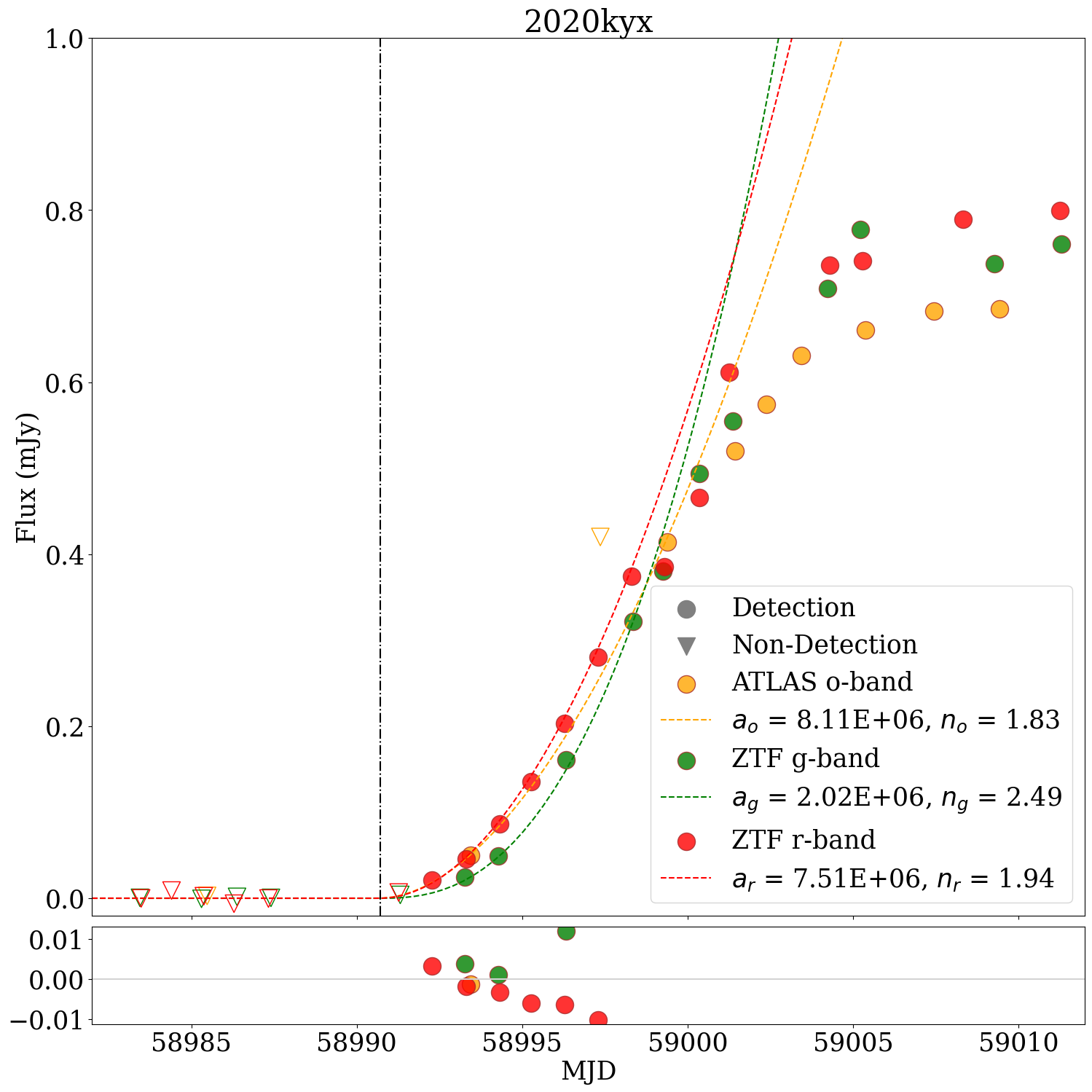
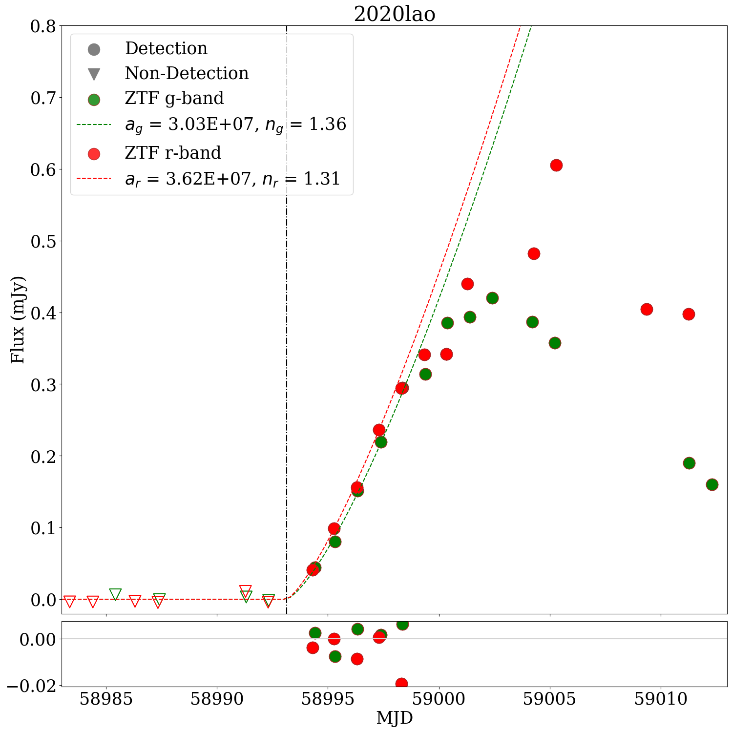
Figure 20: Fireball fits to the light-curve rise for the remaining four SNe Ia and the SN Ic-BL.

where $\alpha$ is a normalizing coefficient, $t_{0}$ is the time of first light and $n$ the index of the power law. We use all available bands for these fits simultaneously, allowing the fit to choose a single $t_{0}$ value for all bands. We determined if a band was viable if there were at least two observations between the estimated $t_{0}$ value and the half-maximum of the light curve. As an example, Figure 7 shows the power-law fitting result for SN 2020jhf. In this case, the ALTAS c-band did not have sufficient data to perform the fit, so it was not considered. The fits for the remaining 4 SNe Ia and the SN Ic-BL are shown in Figure 20 of Appendix A.

For SNe II, we estimated the times of first light by implementing the method presented by Csörnyei et al. (2023). The flux in each photometric band was fitted simultaneously considering the following inverse exponential law,

$$f_{W}(t)=f_{m,W}\left[1-exp\left(-\frac{t-t_{0}}{t_{e,W}}\right)\right],$$ (7)

where $t_{0}$ is the time of first light, $t$ is the time, $f_{m,W}$ the peak flux, and $t_{e,W}$ the characteristic rise time in a specific band, $W$. The fitting procedure considers the depth of the non-detections and the fact that the rise-time of a SN II increases for longer wavelengths (González-Gaitán et al., 2015a). The fits are then connected through $t_{0}$, enabling us to obtain a single estimate considering simultaneously the different photometric bands. Figure 8 demonstrates the exponential fitting on the light curves of SNe 2020nny and 2020jfo. Unfortunately, for SN 2020kjt it was not possible to estimate using Csörnyei et al. (2023) method due to the large gap of ATLAS and ZTF photometry around the explosion time (see Figure 1).

Finally, the SN IIb 2020itj was not fit by any of these methods. Besides the main light-curve peak powered by the radioactive decay of nickel, some SNe IIb show an additional peak at early epochs due to the cooling of the outer layers of the progenitor star that were ejected right after the explosion. SN 2020itj early photometry does not completely show an initial bump, but some signatures: the first few points do not increase in brightness exponentially from zero flux. The first detection of SN 2020itj resembles the early cooling initial bump seen in some type IIb SNe (e.g., Richmond et al. 1994), which makes our method unuseful for determining the time of first light.

The estimated time of first light considering the different implemented methods are summarized in Table 3. For the two SNe without rising light curve fits, we adopt the mid-point estimate value. For the rest, we will use the early light-curve method. The final time of first light is highlighted in bold text. We note that in four cases (SNe 2020jhf, 2020kku, 2020kyx, 2020rlj) the early light-curve method gives an estimate that is earlier that the forced last non-detection. We associate this with the fact that image was not deep enough to properly get a detection but trust the early fit. These are indicated in italics in Table 3. As a comparison with already reported values in the literature, for SN 2020jfo we obtained $t_{0}=58974.72\pm 0.19$ MJD, which is in agreement within uncertainties with the estimated value from Ailawadhi et al. (2023), $t_{0}=58973.1\pm 1.6$, and also with the value used in Teja et al. (2022), $t_{0}=58973.8\pm 0.5$, estimated considering the mid epoch between the last non-detection and the first detection of ZTF.

4.3 Light-curve parameters

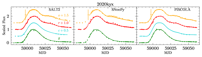
Figure 9: Multi-colour light-curve fits of SN Ia 2020kyx using SALT2 (left panel), SNooPy (max_model—; middle panel) and beautiful PISCOLA (right panel). The ATLAS-$c$ light curve was not included in the SNooPy fit as it produces worse results.

Table 4: SNe Ia light-curve parameters.

		SALT2				SNooPy			PISCOLA
IAU Name	Type	$t_{\rm max}$	$B_{\rm max}$	$x_{1}$	$c$	$t_{\rm max}$	$B_{\rm max}$	$s_{BV}$	$t_{\rm max}$	$B_{\rm max}$	$\Delta m_{15}(B)$	$(B-V)$
2020jgl	Ia	58993.18 $\pm$ 0.01	13.594 $\pm$ 0.002	-0.095 $\pm$ 0.012	0.044 $\pm$ 0.002	58993.024 $\pm$ 0.343	13.605 $\pm$ 0.018	0.967 $\pm$ 0.031	58992.116 $\pm$ 0.245	13.565 $\pm$ 0.011	1.111 $\pm$ 0.018	0.054 $\pm$ 0.013
2020jhf	Ia	58991.77 $\pm$ 0.01	15.375 $\pm$ 0.002	-0.922 $\pm$ 0.009	0.079 $\pm$ 0.001	58991.610 $\pm$ 0.359	15.270 $\pm$ 0.016	0.883 $\pm$ 0.032	58991.283 $\pm$ 1.265	15.773 $\pm$ 0.139	1.137 $\pm$ 0.393	0.250 $\pm$ 0.130
2020kku	Ia	58996.45 $\pm$ 0.10	18.944 $\pm$ 0.014	-1.409 $\pm$ 0.109	0.104 $\pm$ 0.012	58996.294 $\pm$ 0.375	19.013 $\pm$ 0.021	0.836 $\pm$ 0.033	58995.836 $\pm$ 0.348	18.996 $\pm$ 0.022	1.027 $\pm$ 0.072	0.245 $\pm$ 0.046
2020kyx	Ia	59008.48 $\pm$ 0.05	16.445 $\pm$ 0.013	-0.547 $\pm$ 0.054	0.022 $\pm$ 0.009	59008.424 $\pm$ 0.354	16.533 $\pm$ 0.017	0.979 $\pm$ 0.032	59007.233 $\pm$ 0.581	16.642 $\pm$ 0.021	0.914 $\pm$ 0.045	0.272 $\pm$ 0.031
2020rlj	Ia-91bg∗	59088.72 $\pm$ 0.07	18.530 $\pm$ 0.014	-2.814 $\pm$ 0.083	0.247 $\pm$ 0.011	59088.078 $\pm$ 0.354	18.682 $\pm$ 0.017	0.476 $\pm$ 0.032	59087.487 $\pm$ 0.257	18.664 $\pm$ 0.025	2.285 $\pm$ 0.396	0.521 $\pm$ 0.036

Table 5: SNe light-curve parameters obtained with PISCOLA.

		ZTF-$g$		ATLAS-$c$		ZTF-$r$		ATLAS-$o$
IAU Name	Type	$t_{\rm max}$	$m_{\rm max}$	$t_{\rm max}$	$m_{\rm max}$	$t_{\rm max}$	$m_{\rm max}$	$t_{\rm max}$	$m_{\rm max}$
2020itj	IIb	58980.204 $\pm$ 0.412	19.173 $\pm$ 0.039	58980.780 $\pm$ 0.383	18.950 $\pm$ 0.034	58981.753 $\pm$ 0.467	18.805 $\pm$ 0.030	58982.302 $\pm$ 0.649	18.873 $\pm$ 0.042
2020jfo	II	58980.193 $\pm$ 0.408	14.456 $\pm$ 0.017	58980.120 $\pm$ 0.411	14.423 $\pm$ 0.020	58980.147 $\pm$ 1.054	14.405 $\pm$ 0.029	58980.603 $\pm$ 2.244	14.479 $\pm$ 0.040
2020jgl	Ia	58992.846 $\pm$ 0.361	13.734 $\pm$ 0.010	58994.941 $\pm$ 0.479	13.700 $\pm$ 0.014	58994.659 $\pm$ 0.397	13.654 $\pm$ 0.014	58994.863 $\pm$ 0.324	13.938 $\pm$ 0.003
2020jhf	Ia	58992.839 $\pm$ 0.352	15.342 $\pm$ 0.004	58996.254 $\pm$ 0.941	15.392 $\pm$ 0.012	58992.631 $\pm$ 0.927	15.342 $\pm$ 0.011	58991.685 $\pm$ 0.850	15.525 $\pm$ 0.013
2020kjt	II	– –	– –	– –	– –	– –	– –	– –	– –
2020kku	Ia	58995.930 $\pm$ 0.345	19.121 $\pm$ 0.019	58996.682 $\pm$ 0.563	18.987 $\pm$ 0.045	58996.923 $\pm$ 0.496	18.957 $\pm$ 0.019	58996.792 $\pm$ 0.814	19.048 $\pm$ 0.054
2020kyx	Ia	59007.794 $\pm$ 0.815	16.689 $\pm$ 0.011	59009.449 $\pm$ 1.177	16.600 $\pm$ 0.016	59010.178 $\pm$ 1.115	16.643 $\pm$ 0.012	59009.297 $\pm$ 1.569	16.820 $\pm$ 0.017
2020lao	Ic-BL	59002.586 $\pm$ 0.240	17.368 $\pm$ 0.016	59003.107 $\pm$ 0.364	17.166 $\pm$ 0.033	59004.807 $\pm$ 0.839	17.179 $\pm$ 0.018	59005.921 $\pm$ 0.751	17.313 $\pm$ 0.027
2020nny	II	59023.426 $\pm$ 2.037	20.294 $\pm$ 0.073	– –	– –	59024.434 $\pm$ 2.356	20.027 $\pm$ 0.061	59028.879 $\pm$ 1.506	18.863 $\pm$ 0.035
2020rlj	Ia-91bg	59087.800 $\pm$ 0.258	18.759 $\pm$ 0.014	59088.663 $\pm$ 0.314	18.502 $\pm$ 0.019	59090.534 $\pm$ 0.647	18.309 $\pm$ 0.013	59091.718 $\pm$ 0.938	18.352 $\pm$ 0.028

To estimate the light-curve parameters of the SNe presented in this work, we use different SN light-curve fitters. SNe Ia are fitted with SALT2 (Guy et al., 2005, 2007, using the implementation in sncosmo Barbary et al., 2016), SNooPy (Burns et al., 2011) and the updated version 2.0.0 of PISCOLA (Müller-Bravo et al., 2022). SALT2 uses a template-driven approach, modelling the SED of a SN Ia as a function of three light-curve parameters: a global flux scaling ($x_{0}$), time-stretch ($x_{1}$) and colour at maximum light ($c$). SNooPy follows a similar approach, modelling the SED of a SN Ia as a function colour-stretch ($s_{BV}$; Burns et al., 2014), plus other parameters depending on the exact model used. PISCOLA uses a data-driven approach for fitting transient light curves, thus not depending on light-curve parameters, based on Gaussian Processes (GPs; Rasmussen & Williams 2006). We report the results of the SNe Ia fits in Table 12.

The SALT2 template is only trained with normal SNe Ia, so its fits for the 1991bg-like SN 2020rlj is not completely reliable. SNooPy fits were performed using the max_model, applying the $K$-correction versions of the $H3$ template (Hsiao et al., 2007) for normal SNe Ia and the $91bg$ template for 1991bg-like SNe Ia. Only epochs between $-30$ and $+50$ days with respect to optical peak were selected. For SN 2020kyx, we removed the ATLAS-$c$ band to produce better results, while for SN 2020jgl, we removed both ZTF bands for the same reason. PISCOLA fits were performed in flux space using the GP with a Matérn-5/2 kernel (the default procedure), except for SN 2020itj and SN 2020kku, for which an Exponential-Squared kernel was used, and SN 2020nny, which was fitted in logarithmic space, producing better results.

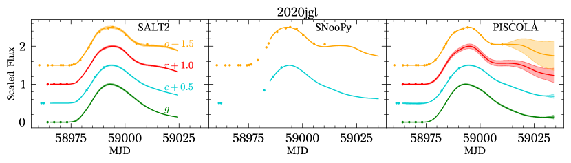
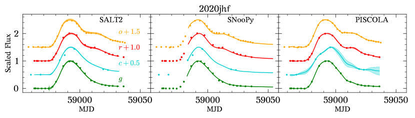
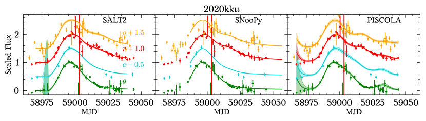
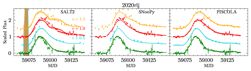
Figure 21: Similar to Figure 9. Summary of the light-curve fits for the remaining four SNe Ia. In the left column we show SALT2 fits, in the central column SNooPy fits, and in the right column fits from PISCOLA. More details in section 4.3.

As an example, in Figure 9, we show the results of the SN Ia 2020kyx fit using the three light-curve fitters. For the directly comparable parameters, such as the time and magnitude of rest-frame $B$-band peak ($t_{\rm max}$ and $B_{\rm max}$, respectively), we see that there are some small differences between the fitters. SALT2 and SNooPy provide similar values of $t_{\rm max}$, while PISCOLA estimates the maximum to be a day earlier. In the case of $B_{\rm max}$, all the fitters produce different results, but within $\sim 0.1$ mag. The different results produced by PISCOLA can be attributed to the relatively flat peaks (see the right panel of Figure 9), although this artefact is a consequence of the photometry. Similar fits for the remaining 4 SNe Ia are showed in Figure 21 of Appendix A.

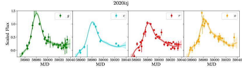
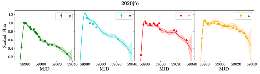
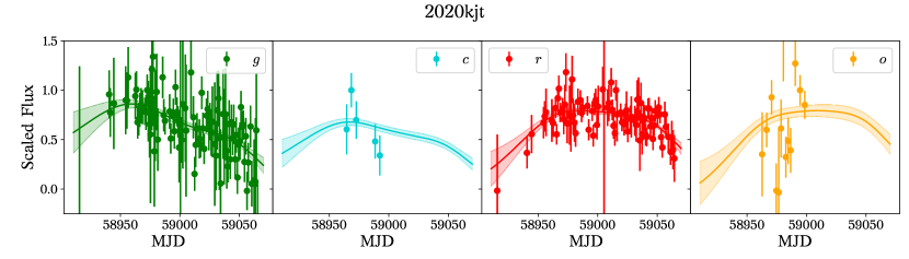
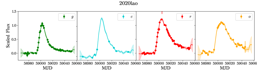
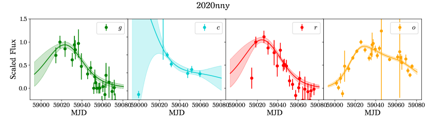
Figure 22: PISCOLA fits to all five CCSNe in our sample.

In addition to the fits of the SNe Ia, given the versatile nature of PISCOLA, we also fit the light curves of the five CCSNe. In Table 13, we report the time of maximum and the peak magnitude for each of the ZTF and ATLAS bands. Note that the values of the SNe II are not completely reliable due to the relatively low quality of the photometry. Furthermore, we do not report values for SN 2020kjt, as the light-curve rise was not observed. All fits are shown in Figure 22 of Appendix A.

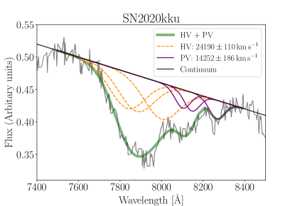
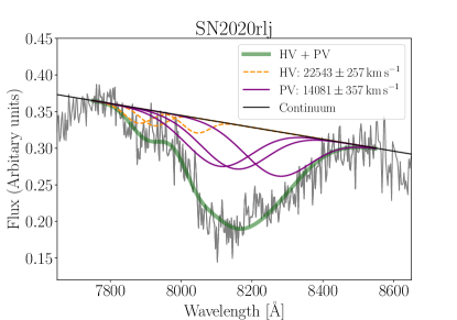
Figure 10: The spectral fitting to the Ca II IR line of the supernovae SN2020kku (left) and SN2020rlj (right). The orange, dashed-line Gaussians account for the Ca II IR triplet of the high-velocity component, while the purple, continuous-line Gaussians for the Ca II IR triplet of the photospheric velocity. The thick, green line is the sum of the high and photospheric velocity components, and finally, the black continuous line indicates the continuum.

4.4 Epochs of the GTC spectra

We determined the epochs of the spectra with respect the estimated time of first light by using the two methods: mid-point and early fit (see section 4.2). Uncertainties in the epochs are estimated accounting for the uncertainty on the estimated time of first light and also the uncertainty of the time at which the spectrum was taken, where we take the time of the middle of the exposure (ranging from 500 to 900 seconds) with an uncertainty of half of the exposure time. Epochs are then transformed to and reported in the restframe in Table 3. The final spectrum dates are highlighted in bold text in the rightmost columns.

From the 10 objects in our sample, we ended up with only two within 48 hours from the estimated first light; 2020jfo at 1.8 days and 2020lao at 2.0 days. Even when SN 2020jfo was one of the two objects that we decided to trigger that had a non-detection earlier than 48 hours (cirterion i in section 2) it ended up being our earliest spectrum. Being a type II SN, the rise time is typically quite short (about a week, see González-Gaitán et al. 2015b), and given the redshift of its host galaxy, the discovery magnitude was -14.8 mag, consistent with a very young SN. SN 2020lao was a SN Ic Broad-Line at -15.9 mag at discovery. Our spectra 2 days after the estimated first light is possibly the earliest spectrum of a SN Ic-BL with no associated GRB ever taken.

Table 6: Rest-frame epochs of the spectra with respect to maximum light (in the $B$ band) and rise time from first light to peak.

SN name	Type	Epoch from maximum	Rise time
2020jgl	Ia	$-$16.16$\pm$0.01	18.74$\pm$1.14
2020jhf	Ia	$-$12.65$\pm$0.01	16.75$\pm$0.20
2020kku	Ia	$-$7.64$\pm$0.10	13.51$\pm$0.87
2020kyx	Ia	$-$13.85$\pm$0.05	17.22$\pm$0.33
2020rlj	Ia-91bg	$-$10.10$\pm$0.07	13.86$\pm$0.42
2020lao	Ic-BL	$-$7.16$\pm$0.23	9.16$\pm$0.29
2020itj	IIb	$-$8.91$\pm$0.40	18.4$\pm$0.79

Following these two earliest spectra, we have the five SNe Ia, three with epochs from two to four days (2020jgl at 2.6d, 2020kyx at 3.4d, and 2020rlj at 3.8d) and two more with spectra from four to six days after the estimated time of first light (2020jhf at 4.1d and 2020kku at 5.9d). SN 2020jhf was the other candidate for which we did not follow the first criterion. In Figure 1, we show a forced-photometry detection in the ZTF $i$-band that, if available when we had to trigger, would have made us discard this object. On the other hand, it would have been a good target one day earlier, and assuming the trigger executed at the same time of the night, we would have got a spectrum 3.1d after first light, the fourth in our sample.

SN 2020itj spectrum was obtained nine days after first light. The early light curve of this type IIb SN does not perfectly follow an exponential decline towards the time of first light, but instead, there is a reminiscent of the bright cooling phase typical for some SNe IIb (see Figure 1). We discuss this further in section 5.1.

The remaining two objects, SN 2020nny and 2020kjt, have epochs of sixteen and sixty days, repectively, after the estimated first light. We consider these failures of our method. In both cases the SN was of type II. SN 2020kjt was discovered during the plateau phase at a magnitude 20.45 mag, close to the median magnitude limit of the ZTF survey. Fluctuations in the difference photometry made Forster et al. (2020) report the detection with a close $r$-band non-detection of 20.65 mag 21 hours earlier, but they both turned out to be forced-photometry detections. Similarly, SN 2020nny was discovered at what turned out to be the peak of the light-curve at 19.1 mag in $r$, with a $3\sigma$ non-detection of 20.3 mag in the $g$-band reported 27 hours earlier, which also resulted in a detection with forced-photometry.

In addition to the epochs with respect to the estimated time of first light, we also report the epoch with respect to maximum light for all type I SNe. For SNe Ia we used the epoch of the peak as measured with SALT2 (see section 4.3), while for the SN Ic-BL and the SN IIb we used the value from PISCOLA measured in the $g$-band. Table LABEL:table:epsp reports the resulting rest-frame epochs. SN 2020jgl is our SN Ia with the earliest spectrum from maximum light, at an epoch of $-$16.2 days. The following two earliest spectra, from SNe 2020jhf and 2020ky, are at $-$13 and $-$12 days, which are also significantly early, but not as early as we had hoped to achieve with our programme. Spectra for SNe 2020rlj and 2020kku are at $-$10 and $-$7 days, respectively, which are routinely obtained by spectroscopic SN follow-up programmes such as ePESSTO+ (Smartt et al., 2015). In Table LABEL:table:epsp, we also report the corresponding rise-times for each SN. For SNe Ia, these range from 13 to 19 days, which compared to a typical distribution from Miller et al. (2020b), it highlights that indeed our estimated times of first light may not really be approximate to the explosion epochs.

From all the above, we conclude that the configuration of the discovery survey telescope used in this work (P48, 1.22 m diameter), even with a great wide-field camera (ZTF, 47 sq. deg), is not deep enough to cover the early epochs at the redshift range of our sample ($z>0.01$). At these redshifts, obtaining spectra of young SNe (within 48 hours of explosion) is impossible if their brightness during the earliest epochs is significantly below the survey’s limiting magnitude. This is further discussed in section 6.

4.5 Expansion Ejecta Velocities

Table 7: Expansion Velocities.

Type Ia
	Ca II IR triplet	Ca II IR triplet - HV	Ca II H&K	Si II $\lambda$5792	Si II $\lambda$6533
2020jgl	35,802 $\pm$ 415	$-$	5,721 $\pm$ 991	18,837 $\pm$ 373	21,096 $\pm$ 234
2020jhf	12,075 $\pm$ 165	20,125 $\pm$ 121	17,984 $\pm$ 689	11,571 $\pm$ 397	12,557 $\pm$ 140
2020kku	14,252 $\pm$ 186	24,190 $\pm$ 110	24,211 $\pm$ 773	13,805 $\pm$ 366	15,536 $\pm$ 765
2020kyx	22,563 $\pm$ 1195	$-$	28,456 $\pm$ 836	13,177 $\pm$ 199	14,995 $\pm$ 185
2020rlj	14,081 $\pm$ 357	22,543 $\pm$ 257	15,579 $\pm$ 233	13,633 $\pm$ 174	14,183 $\pm$ 253
Type II
	H$\alpha$	H$\beta$	Na I D $\lambda$5893	Fe II $\lambda$5018	Fe II $\lambda$5169
2020kjt	5,909 $\pm$ 151	4,499 $\pm$ 38	3,232 $\pm$ 90	3,120 $\pm$ 40	3,078 $\pm$ 50
2020nny	9,266 $\pm$ 1021	9,008 $\pm$ 64	8,963 $\pm$ 8	6,839 $\pm$ 88	7,208 $\pm$ 171
Type IIb
	H$\alpha$	He I $\lambda$5876	He I $\lambda$7065
2020itj	10,586 $\pm$ 318	6,692 $\pm$ 100	4,913 $\pm$ 20

We have estimated the expansion velocities in the GTC spectra of our ten SNe. We present here the results for eight of them, while those for SN 2020jfo were presented in Ailawadhi et al. (2023) and those for SN 2020lao will be presented in Stritzinger et al. (in prep.).

For SNe Ia, we have used a modified version of the code Spextractor (Papadogiannakis, 2019) to measure velocities and pseudo-equivalent widths pEWs. This modified version presented in Burrow et al. (2020) has enabled the downsampling of spectral information while ensuring the conservation of the number of photons, in order to reduce computational cost. Additionally, adjustments were made to produce a more representative GP regression model and smoothing for a given spectrum so that it returns reliable measurements of velocities and pEWs. Thus, the code calculates those velocities by converting the wavelength shifts of absorption lines into velocities using the relativistic Doppler formula provided in Equation 6 in Blondin et al. (2006). The ejection velocity is determined by measuring the flux minima of the absorption lines of the spectral features with respect to its rest wavelengths, which are provided and outlined in Table 5 of Folatelli et al. (2013). In our analysis, we focused on specific spectral features that are easily identifiable and isolated in the spectra of SN Ia. These features, given in Table LABEL:table:velocities, include the absorption lines of Ca II IR triplet, Ca II H&K, Si II $\lambda$6533, and Si II $\lambda$5792, as well as their calculated expansion velocities.

There are three cases (SN2020jhf, SN2020kku, and SN2020rlj) where the Ca II IR triplet region (8498 Å, 8542 Å, 8662 Å) presents high-velocity features on top of the photospheric features. To calculate the contribution of both regimes, we fit six Gaussians at the same time: three to estimate the photospheric velocity (PV) and three for the high velocity (HV) component. Figure 10 shows an example for SNe 2020kku and 2020rlj. We force the $\sigma$ value and the amplitude of the three Gaussians of the PV components to be equal, and we do the same for the HV components. In addition, a minimum difference of 2000 km s^-1 between PV and HV was set. All measured velocities are presented in the first rows of Table LABEL:table:velocities.

For CCSNe, type II and IIb, we computed the relativistic velocities using an alternative method independent from Spextractor. First, we choose two neighbouring regions for each spectral line, one on each side of the line. Within these regions, the upper and lower wavelength limits were determined by analyzing the derivative of the flux with respect to the wavelength. Specifically, the numerical derivative was calculated across the region of interest, and the wavelength corresponding to the maximum change in the slope (the maximum or minimum of the derivative) was identified. This point represents the location where the flux transitions most sharply, helping to define the boundaries of the feature. Once the wavelength range for the feature is established, a pseudo-continuum is defined between the two limits and the spectrum is normalized. Finally, a Gaussian profile is fitted to the normalized flux to determine the central wavelength of the feature. Using the Doppler formula with relativistic corrections, we computed the velocities relative to the known rest wavelength of each spectral line. For determining the errors, the same process was performed a hundred times, applying a shift to the feature limits. The standard error is calculated as the dispersion in the hundred additional velocities. We report the H$\alpha$ and H$\beta$ features for both H-rich (II) and H-poor (IIb) CCSNe. Additionally, we report Fe II lines together with Na I for SNe II. For the SN IIb 2020itj we report the He I lines ($\lambda 5876$ and $\lambda 7076$). All velocities are prestented in Table LABEL:table:velocities.

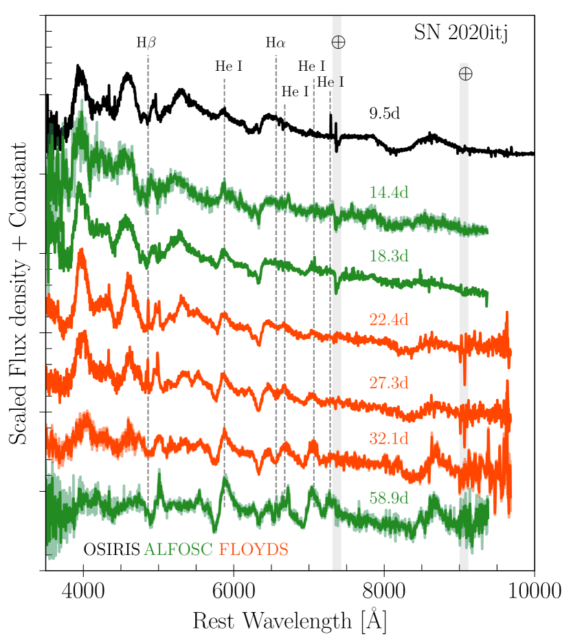
Figure 11: Spectral sequence of the type IIb SN 2020itj from 8.7 to 60.8 d from explosion in the rest-frame. The phases are labelled on the right. Each spectrum has been corrected for Milky Way reddening, put int he rest-frame, and shifted vertically by an arbitrary amount for presentation. The colour of the spectra represents the different instruments used to obtain the data. The vertical dashed lines indicate the rest position of the strongest lines. Telluric absorption lines are highlighted with grey lines ($\oplus$ symbol).

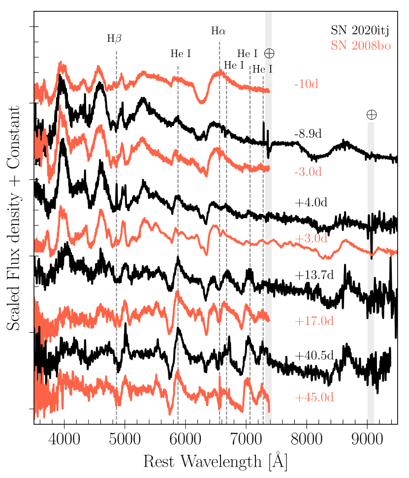
Figure 12: Spectral comparison of SN 2020itj with the type IIb SN 2008bo (Modjaz et al., 2014; Shivvers et al., 2019). Each spectrum has been corrected for Milky Way reddening and shifted vertically by an arbitrary amount for presentation. The vertical dashed lines indicate the rest position of the strongest lines. Telluric absorption lines are highlighted with grey lines ($\oplus$ symbol).

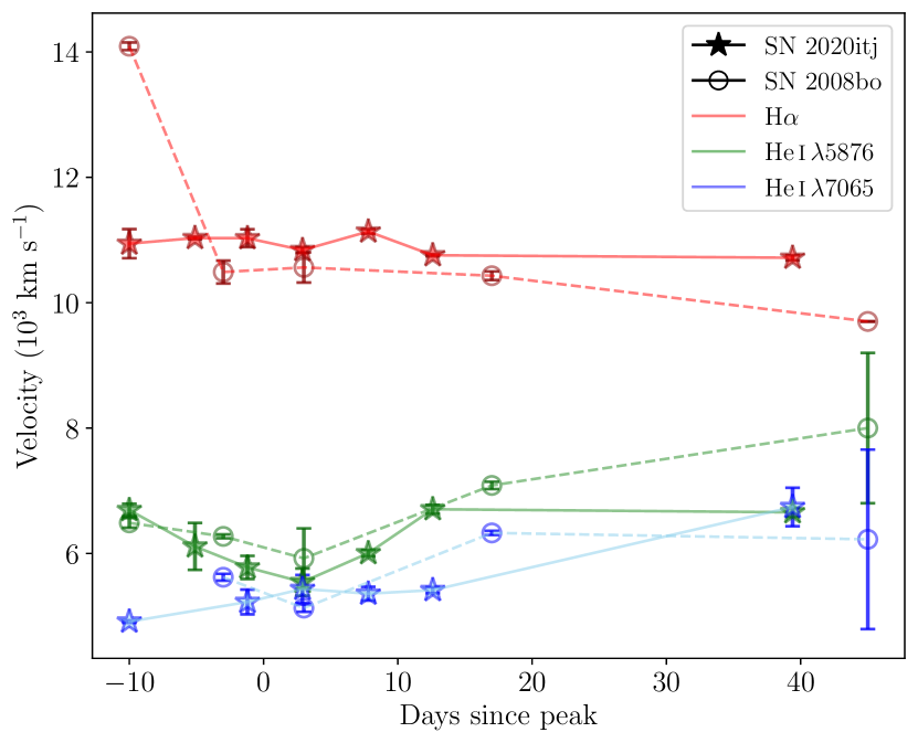
Figure 13: Evolution of expansion velocities of SN 2020itj and SN 2008bo derived from the absorptions of the strongest lines.

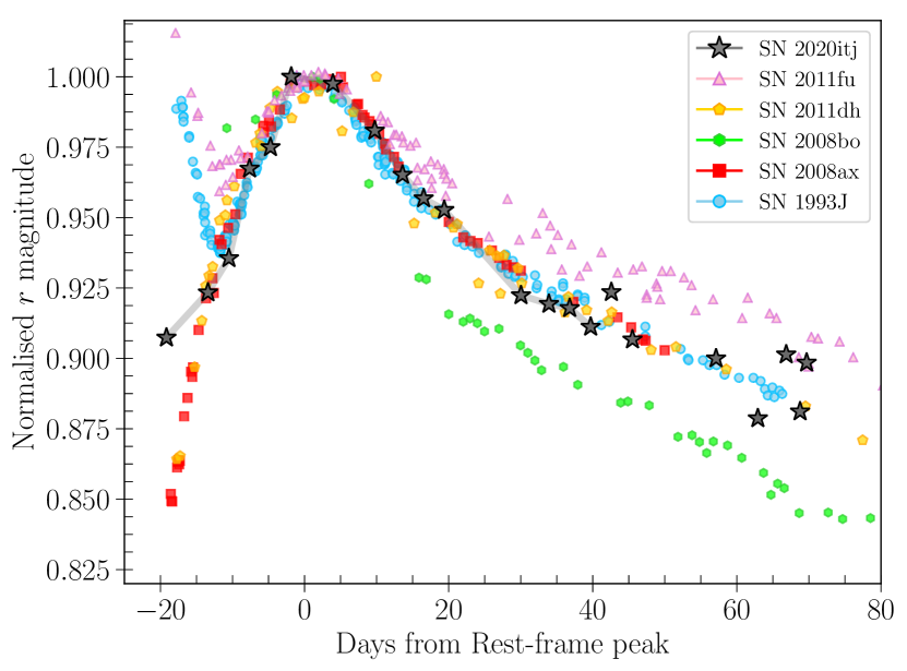
Figure 14: Photometric comparison of SN 2020itj with well-studied SNe IIb. The light curves have been normalised to the peak. The photometry for SNe 1993J, 2011dh and 2011fu is in the $R-$band.

5 Interesting objects

From the ten objects in our sample, we succeeded in two cases to obtain a spectrum within 48h from the estimated time of first light. Further study of these two objects is left for dedicated publications: the GTC-OSIRIS spectrum of SN 2020jfo has been already presented in Ailawadhi et al. (2023), and the spectrum of SN 2020lao together with a full characterization of the SN will be presented elsewhere (Stritzinger et al. in prep.).

From the remaining objects, although not fulfilling our initial goals, we consider SN 2020itj and SN2020jgl, the most interesting found. For these objects we complemented the ATLAS and ZTF photometric data with the UBVg’r’i’ bands from Las Cumbres Observatory (Howell et al., 2016), and present below these and extended spectral sequences form other sources.

5.1 SN 2020itj

SN 2020itj was initially classified as a type Ib SN based on spectral matching (Galbany et al., 2020e), but a more detailed analysis of the spectra and light curves presented below suggests that it is, in fact, a type IIb SN. The middle panel of the SN 2020itj Figure 1 shows that the GTC spectrum was obtained within 24 hours from the reported non-detection, which turned out to be about 9.5 days after the time of first light, as estimated from forced photometry. This implies some critical information was missed in the early phases. However, the light curve in the $r-$band shows a hint of an initial peak, i.e. a double-peaked structure, while as we show below the spectral evolution goes from a spectrum with H lines (at 9.5 days) to a spectrum dominated by He I (at $\sim 59$ days). These two properties are commonly seen in SNe IIb.

Figure 11 shows our spectrum and further six follow-up spectra obtained from 14.4 to 59.8 days from the explosion. Details of the spectroscopic observations of SN 2020itj can be found in Table 11. Our first spectrum at 9.5 days is dominated by strong lines of H$\alpha$, He I $\lambda 5876$, Ca II (H&K and NIR triplet) and Fe II (the ”W” feature produced by the blending of Fe II; Liu et al. 2016). H$\alpha$ is visible all the time, from 9.5 to 58.9 days. At 24 days, He I $\lambda 6678$ and 7065 start to be visible. As time passes, H$\alpha$ becomes weak, and the He I lines become stronger. Finally, after 30 days, the spectra start to be dominated by He I lines. In Figure 12, we compare SN 2020itj and the best spectral match object obtained with a typical well-studied type IIb SN 2008bo (Modjaz et al., 2014; Shivvers et al., 2019). The first spectrum of SN 2020itj (at $-9$ days around peak) is identical to SN 2008bo at $-3$ days. Both objects have the ”W” Fe II feature, He I $\lambda 5876$ and a weak detection of H$\alpha$. As can be seen, at all epochs, the evolution of these objects is similar. Although SN 2020itj does not have spectra before $-10$ days, we expect that early on, it behaves similarly to SN 2008bo, i.e., a spectrum dominated by H lines (first spectrum in the Figure).

The expansion velocities of H$\alpha$, He I $\lambda 6678$ and 7065, derived from the minima of the P-Cygni absorptions for SN 2020itj and SN 2008bo are presented in Figure 13. As expected, the highest velocity for both objects corresponds to H$\alpha$, with an average velocity of $\sim 11000$ km s^-1, while the lowest velocities correspond to He I lines with values between 5000 and 6000 km s^-1. The velocities for these SNe are much lower than those measured for well-observed SNe IIb, such as SN 1993J, SN 2008ax, (see Taubenberger et al., 2011), but similar to those found by Folatelli et al. (2014) for flat-velocity SNe IIb. Comparing these flat-velocity SNe with SN 2020itj and SN 2008bo, we see that their velocity evolution is identical: flat velocities before 10 days from the peak and an increased velocity after that. These flat velocities have been attributed to a dense shell in the ejecta (Folatelli et al., 2014).

In Figure 14, we compare the $r$-band light curve of SN 2020itj with the well-observed type IIb SNe 1993J (Richmond et al., 1994; Barbon et al., 1995), 2008ax (Pastorello et al., 2008), 2008bo (Bianco et al., 2014), 2011dh (Sahu et al., 2013; Zheng et al., 2022), 2011fu (Kumar et al., 2013; Morales-Garoffolo et al., 2015). To analyse the photometric behaviour of SN 2020itj and the comparison sample, we normalise their magnitudes. Overall, the light curve of SN 2020itj has a similar shape to SNe 2008ax and 2011dh; however, the first point of SN 2020itj deviates from the expected rise, suggesting that this first point corresponds to an initial peak (shock cooling), which may resemble those observed in SN 1993J and SN 20011fu. In fact, the light curves of SN 1993J and SN 2020itj match at all epochs. The only difference is the pronounced initial peak observed in the former. Despite SN 2008bo’s spectral evolution being similar to SN 2020itj’s, their photometric behaviour is slightly different. After the peak, SN 2008bo has a faster decline rate. However, the spectral and photometric evolution of SN 2020itj is consistent with that of SNe IIb.

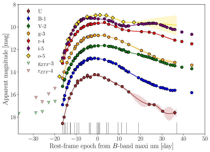
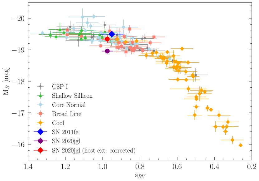
Figure 15: Top: SN 2020jgl multi band light-curve from ZTF, ATLAS and Las Cumbres Observatory network of telescopes together with a GP interpolation for clarity. Vertical lines at the bottom represent the epochs at which we obtained optical spectra. Bottom: Absolute magnitude vs color-stretch parameter diagram populated with Carnegie Supernova Project I SNe Ia. colored by their position in the Branch diagram (see Figure 16). The normal SN2011fe is indicated with a blue dot, while SN 2020jgl is represented with a purple dot or a red dot, depending on whether the host galaxy extinction correction is applied.

5.2 SN 2020jgl

SN 2020jgl is a SN Ia with average light-curve parameters, as reported in Table 12. To refine and provide more precise measurements, we supplemented ZTF and ATLAS photometry with $UBVgri$ photometry from the Las Cumbres Observatory network of telescopes and repeated the light-curve fits with SNooPy using the EBV_model2. All the photometry available and the new SNooPy fit are shown in Figure 15 and reported in Table 12. This new fit gives a $T_{\rm max}$ = 58992.924 $\pm$ 0.34, which is 0.1 days earlier than the value previously reported for SNooPy in Table 12, and a light-curve stretch parameters $\Delta m_{15}(B)$ = 1.026 $\pm$ 0.061 mag and $s_{BV}$ = 0.975 $\pm$ 0.030, also consistent with previous results. The rise time to optical maximum with this new time of maximum is $t_{\rm rise}=18.49$ days, consistent with the average values measured for SNe Ia ($18.98\pm 0.54$ days; Firth et al., 2015). This time, with a light-curve for the $B$-band available, the peak magnitude is $m_{B}$ = 13.522 $\pm$ 0.034 once corrected for galactic extinction and k-corrected using the updated Hsiao et al. (2007) SN Ia template. At the redshift of the SN and considering the distance modulus obtained from SNooPy, 32.480 $\pm$ 0.093 mag, it corresponds to an absolute peak magnitude of $M_{B}$ = $-$18.958 $\pm$ 0.034. Once a correction for the host galaxy extinction of $EBV\_host=0.192\pm 0.060$ mag and an $R_{V}=2$ is included, the peak absolute magnitude results $M_{B}$ = $-$19.342 $\pm$ 0.116 mag. Figure 15 also shows a peak magnitude vs. stretch-color parameter diagram populated with all Carnegie Supernova Project I SNe Ia (CSP; Krisciunas et al., 2017), the typical normal SN Ia 2011fe, and our two measurements for SN 2020jgl with and without accounting for host galaxy extinction.

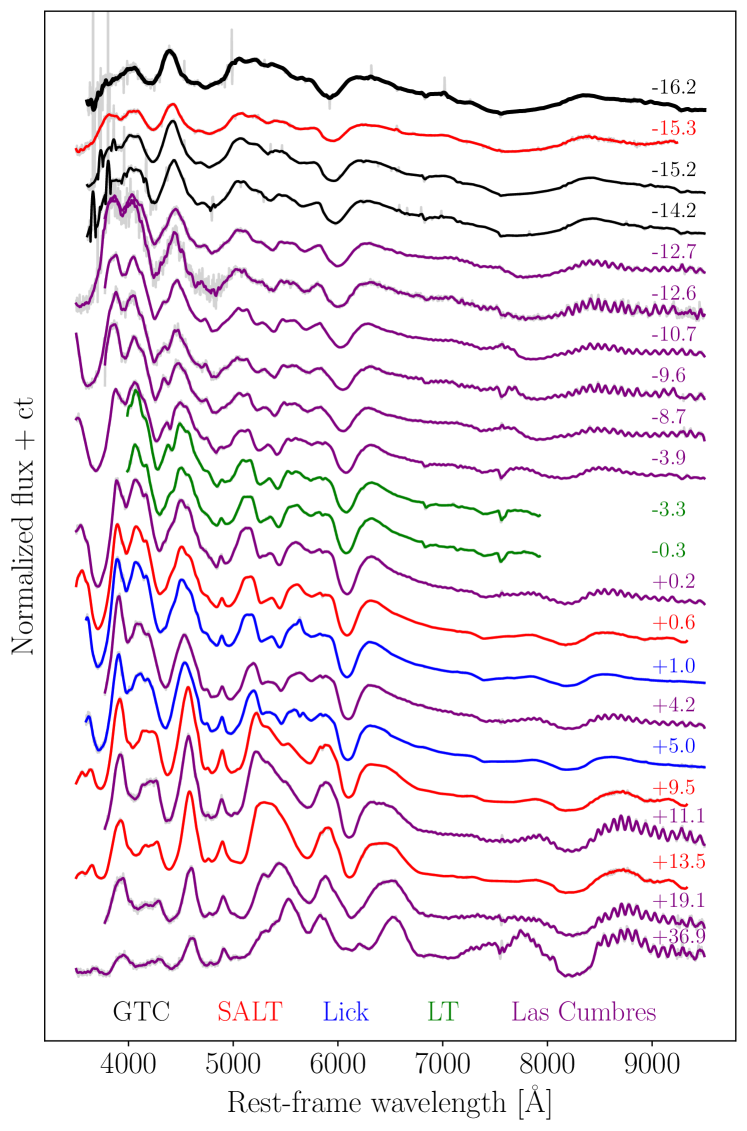
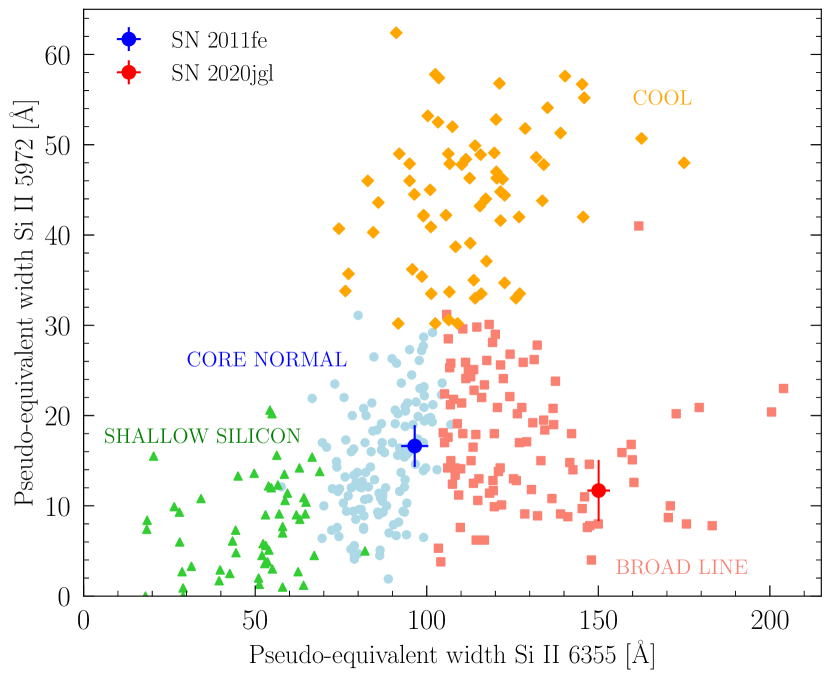
Figure 16: Top: Spectral sequence of SN 2020jgl from various ground-based telescopes, sorted by epoch (earliest to latest). Bottom: Branch diagram of SiII $\lambda$5972 and $\lambda$6355 pseudo-equivalent widths, including CSP and CfA SN Ia samples. SN2020jgl is in the Broad Line region; SN2011fe included for reference.

As mentioned above, we started a spectroscopic follow-up campaign for SN 2020jgl using a number of telescopes: the 10.1m GTC and the 2m Liverpool Telescope (LT) at the Roque de Los Muchachos observatory, the 3m Shane telescope at Lick observatory, the 9.2 Southern African Large Telescope (SALT), and the 2m Las Cumbres Observatory telescope at the Siding Spring observatory through the Global Supernova Project. Figure 16 shows all 22 optical spectra obtained for the SN, ranging from $-$16.2 to +36.9 days from the epoch of maximum light. Details of the spectroscopic observations of SN 2020itj can be found in Table 13.

The main spectroscopic features defined in Folatelli et al. (2013) were analyzed using Spextractor (Papadogiannakis, 2019; Burrow et al., 2020) providing an estimate of the pseudo-equivalent width ($pEW$), velocity ($v$) and depth ($d$). Results are reported in Table 14. Figure 16 also presents the Branch et al. (2006) diagram, using the $pEW$ of the two main Silicon features in the optical. The diagram includes the results for SN 2011fe and SN 2020jgl, and is populated with CSP I and II measurements from Morrell et al. (2024) and Center for Astrophysics (CfA) measurements from Blondin et al. (2012). While SN 2011fe falls in the Core Normal region, SN 2020jgl is classified as a Broad Line SNe Ia according to the diagram. The absolute magnitude vs light-curve width diagram previously presented in Figure 15 also shows the CSP I SNe Ia colored by the spectral subgroups defined in this Branch diagram. We can clearly see how the groups fall in different regions of the relation, with some overlap. SN 2011fe falls in the middle of the Core Normal SNe, and SN 2020jgl is surrounded by both Core Normal and Broad Line dots.

SN 2020jgl was initially triggered for being a good candidate for the Hubble Space Telescope (HST) Supernovae in the near-InfraRed Avec Hubble (SIRAH; Jha et al. 2020) project, under which two WFC3/IR spectra were obtained. We additionally obtained one near-infrared (NIR) spectrum with the Espectrógrafo Multiobjeto Infra-Rojo (EMIR) mounted on the GTC, and two more spectra with the SpeX spectrograph mounted on the 3.2m NASA Infrared Telescope Facility (IRTF) on Mauna Kea observatory, to complement HST data. Since this is not the goal of this paper, these NIR spectra won’t be presented here but elsewhere (Pierel et al. in prep.).

5.2.1 Spectral comparison to other early SNe Ia

In order to assess how early is our earliest SN 2020jgl spectrum, we compared that to publicly available spectra of the other SN Ia discovered early. We obtained spectra from the Weizmann Interactive Supernova Data Repository (WISeREP) of several SNe Ia for which early spectra ($<-14$ days) have been reported: SN2009ig (Foley et al., 2012), SN 2011fe (Zhang et al., 2016), SN 2012cg (Silverman et al., 2012), SN 2013dy (Zheng et al., 2013), SN 2015F (Cartier et al., 2017), SN 2017cbv (Hosseinzadeh et al., 2017; Burke et al., 2022), SN 2019np (Burke et al., 2022), SN 2019ein (Pellegrino et al., 2020), SN 2019yvq (Miller et al., 2020a; Burke et al., 2021). SN 2020nlb (Williams et al., 2024) SN 2021hpr (Zhang et al., 2022) SN 2021aefx (Hosseinzadeh et al., 2022), SN 2023bee (Wang et al., 2024), and SN 2024epr (Hoogendam in prep.).

Table 8: Rest-frame epochs of the spectra with respect to maximum light (in the $B$ band) and rise time from explosion to peak.

SN name	Galaxy	redshift	Epoch	method	Ph. velocity
2009ig	NGC 1015	0.008769	$-$14.4	Poly	21,975$\pm$947
2011fe	NGC 5457	0.000804	$-$15.9	Poly	15,913$\pm$27
2012cg	NGC 4424	0.001458	$-$14.8	Poly	22,441$\pm$45
2013dy	NGC 7250	0.003889	$-$16.0	Poly	17,810$\pm$284
2015F	NGC 2442	0.004890	$-$14.4	Poly	12,937$\pm$379
2017cbv	NGC 5643	0.003999	$-$17.5	SNooPy	22,454$\pm$6,659
2019np	NGC 3254	0.004520	$-$16.0	SNooPy	15,143$\pm$595
2019ein	NGC 5353	0.007755	$-$14.0	SALT2	23,698$\pm$33
2019yvq	NGC 4441	0.00908	$-$14.4	Poly	21,074$\pm$476
2020nlb	NGC 4382	0.002432	$-$16.1	SNooPy	14,991$\pm$438
2021hpr	NGC 3147	0.009346	$-$14.2	Poly	21,164$\pm$632
2021aefx	NGC 1566	0.005017	$-$16.6	Poly	27,840$\pm$255
2023bee	NGC 2708	0.006698	$-$15.7	SALT3	24,381$\pm$321
2024epr	NGC 1198	0.005310	$-$16.7	SNooPy	20,572$\pm$504

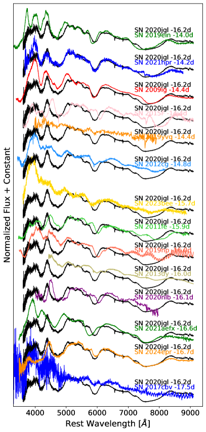
Figure 17: SN 2020jgl spectrum, the earliest presented in this work, compared to spectra from other SNe Ia with reported very early ($<-14$ days) spectra.

Table LABEL:table:earlysp lists all SNe, their host galaxies and redshift from NED, and epochs obtained from the references above, using different methods, or estimated from maximum-light and spectral epochs. We also run Spextractor to measure the Si II $\lambda$6355 velocity, which is also reported in the Table. In Figure 17 we show how all these early spectra sorted by epoch and compared to our earliest SN 2020jgl at an estimated epoch of $-$16.2 days. Looking at the Figure, it is very clear SNe Ia are quite heterogeneous in terms of Si II velocity, which is a proxy for the photospheric velocity. SN 2021aefx is the SN with the highest velocity, more than 27,000 km s^-1 at $-16.6$ days, and SN 2020nlb is the one with the lowest velocity, about 15,000 km s^-1 at $-16.1$ days. While SN 2020jgl had a photospheric velocity of 21,044$\pm$116 km s^-1 (see section 4.5), there are 8 SNe with higher and 6 with lower velocities. SN 2024epr show significant resemblance to SN 2020jgl at those epochs, in all the optical range except at bluer wavelengths than 4500 Å. It is also remarkable the large Ca NIR $pEW$ of SN 2020jgl, only SN 2019ein and SN 2024epr present larger values.

A more quantitative analysis of the early epochs of SNe Ia will be a matter for a dedicated study. Here, we just conclude that the SN 2020jgl GTC spectrum presented in this work contributes to increase the sample of early SN Ia spectra at epochs $<14$ days from the epoch of maximum light.

6 Summary and conclusions

Table 9: Earliest epochs able to be detected as a funciton of SN redshift, $s_{BV}$, and telescope/instrument magnitude limit.

redshift	$M_{lim}$	$\Delta(t_{1st-max})$	$\Delta(t_{1st-max})$	$\Delta(t_{1st-max})$
		$s_{BV}=0.8$	$s_{BV}=1.0$	$s_{BV}=1.2$
mag lim 20.5 (ZTF)
z=0.001	-7.66	-14.97	-17.43	-20.00
z=0.002	-9.17	-14.83	-17.28	-19.86
z=0.005	-11.16	-14.60	-17.01	-19.55
z=0.01	-12.68	-14.30	-16.71	-19.24
z=0.02	-14.20	-13.70	-16.05	-18.53
z=0.03	-15.09	-13.30	-15.61	-18.05
mag lim 21.5 (KMTNet)
z=0.002	-8.17	-14.93	-17.39	-19.96
z=0.005	-10.16	-14.72	-17.14	-19.69
z=0.01	-11.68	-14.52	-16.93	-19.47
z=0.02	-13.20	-14.12	-16.53	-19.06
z=0.03	-14.09	-13.74	-16.09	-18.59
mag lim 22.5 (ATLAS)
z=0.005	-9.16	-14.83	-17.28	-19.86
z=0.01	-10.68	-14.66	-17.08	-19.62
z=0.02	-12.20	-14.42	-16.83	-19.37
z=0.03	-13.09	-14.15	-16.57	-19.10
mag lim 23.5 (DES)
z=0.005	-8.16	-14.93	-17.39	-19.96
z=0.01	-9.68	-14.77	-17.21	-19.78
z=0.02	-11.20	-14.60	-17.01	-19.54
z=0.03	-12.09	-14.45	-16.86	-19.39
mag lim 24.5 (LSST)
z=0.01	-8.68	-14.89	-17.34	-19.91
z=0.02	-10.20	-14.71	-17.14	-19.69
z=0.03	-11.09	-14.61	-17.02	-19.56

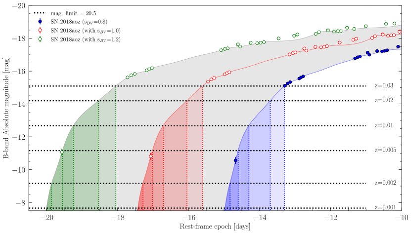
Figure 18: Light-curve simulation based on the observed light curve of SN 2018aoz, a SN with a color-stretch parameter $s_{BV}=0.8$. The original light curve is shown (in blue) alongside simulated versions stretched to represent $s_{BV}$ values of 1.0 (in red) and 1.2 (in green). Horizontal lines indicate the minimum observable magnitude at several redshifts of a telescope-instrument system with a magnitude limit of 20.5 mag.

We have presented the results of a campaign using the Optical System for Imaging and Low-Intermediate-Resolution Integrated Spectroscopy (OSIRIS) mounted on the 10.1m Gran Telescopio de Canarias (GTC) with the goal of obtaining spectroscopy of infant SNe within 48 hours of first light. We successfully acquired data for ten SNe, spanning from 1.2 to 59.4 days after first light. Although only two of the ten spectra were obtained within the first 48 hours, half were captured within the first four days. Possible reasons for this success ratio are discussed below.

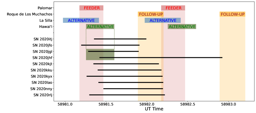
Figure 19: Representation of the nighttime hours at Palomar, where the ZTF survey discovers new SN candidates, and at La Palma, the location of the GTC telescope used for our early spectroscopy program. SN 2020jgl and SN 2020jhf were discovered by the ATLAS unit in Mauna Loa, Hawai’i, and we have also shaded the nighttime hours for this location for these two objects. Horizontal lines for each of the ten SNe in our sample connect the time of discovery with the time the spectra were obtained. Additionally, the nighttime hours at La Silla in Chile and Hawai’i are shown in blue and green, respectively, illustrating how faster follow-up could have been achieved from those locations. This representation corresponds to May 2020, when our GTC program began.

Supplementing the GTC spectra with public photometry from the ZTF and ATLAS surveys, we performed a comprehensive characterization of these ten SNe, providing estimates for the time of first light, time of maximum light, light-curve parameters, and host galaxy extinction. Using these parameters, we determined the epochs of our spectra relative to both the time of first light and maximum light. Supernova typing was conducted using SNID, identifying five Type Ia, three Type II, one Type IIb, and one Type Ic-BL. The photospheric velocities of the main spectral features were measured and reported for all ten spectra in our GTC sample. Finally, we presented a short more in depth analysis of two SNe: SN IIb 2020itj and SN Ia 2020jgl, including photometry and spectroscopy from dedicated follow-up campaigns.

Given our low success rate (20%) relative to the initial goals of the project, we discuss two possible factors that have not allowed us to obtain earlier SN spectra: (i) the time of first light is not necessarily the time of explosion due to the depth of the discovery survey and the distance to the SN; and (ii) the difference in longitude between the discovery telescope and the classification spectroscopy telescope introduces a lower limit on the epoch of the first spectrum.

The time of first light is defined as the moment when a SN becomes bright enough to be detected by a specific telescope and instrument configuration. For instance, a SN may be visible to a large-aperture telescope with a high-efficiency instrument, while a smaller-aperture telescope may fail to detect it. Similarly, due to higher brightness, earlier epochs of a SN in a nearby galaxy (lower redshift) can be detected compared to one in a more distant galaxy using the same telescope configuration. To visually illustrate these two effects, we present an exercise based on SN 2018aoz (Ni et al., 2022), a SN discovered just an hour after first light, with a color-stretch parameter $s_{BV}=0.8$. Figure 18 shows the original light curve of SN 2018aoz alongside two additional light curves representing the same SN, but stretched to simulate SNe with $s_{BV}$ values of 1.0 and 1.2. It is evident that the epochs at which the SN light reaches specific absolute magnitudes vary by a few days across the three light curves. For example, an absolute magnitude of $-10$ is reached at $-15$, $-17$, and $-19$ days, respectively. Assuming a magnitude limit for the discovery survey, horizontal lines in the figure represent the detection thresholds for a telescope-instrument system at various redshifts. The figure shows an example for a magnitude limit of 20.5 mag, comparable to ZTF. Table 9 provides the corresponding limits for surveys with magnitude limits as deep as 24.5 mag, representative of other current and future surveys (e.g., KMNet, Kim et al. 2016; ATLAS, Tonry et al. 2018; DES, Dark Energy Survey Collaboration et al. 2016; LSST, Ivezić et al. 2019). The intersections of the light curves and horizontal lines for different redshifts define the earliest epochs at which a SN with a specific $s_{BV}$ can be observed. For example, a SN with $s_{BV}=1.0$ at a redshift of 0.01 would not be visible earlier than $-17$ days using a system with a magnitude limit of 20.5 mag. Accounting for the time required to process the discovery image, report it to the community, and set up spectroscopic observations, this illustrates the challenges of obtaining spectra of SNe Ia earlier than $-17$ days. It is important to note that the first detection, or first light, is not equivalent to the explosion epoch for a SN observed with a given instrument. The first detection merely indicates the moment the SN becomes just bright enough to surpass the detection limit. This was demonstrated in our program in several cases: even with rapid triggering, the SN was not always at an early phase in forced-photometry light curves, as this method typically provides deeper limits. The discrepancy between the explosion time and the first light imposes significant constraints on acquiring spectra at the earliest SN epochs. This, in turn, limits our ability to study the first few hours after the explosion and to place constraints on the properties of progenitor systems.

On the other hand, aside from the ability to detect the faint initial epochs of a SN, the physical location of the telescope performing the spectroscopic observation relative to the discovery telescope plays a significant role. In our case, most targets were identified by ZTF, a survey conducted with the P48 telescope at the Palomar Observatory in California, USA, with the exception of a couple reported by the ATLAS unit at Mauna Loa, Hawai’i, USA. The spectroscopic classification was performed in all cases using the GTC at the Roque de Los Muchachos Observatory in La Palma, Spain. Due to the longitude difference between these observatories, and depending on the time of year, there is a delay of 7 to 12 hours between the end of the night at Palomar and the start of the night at La Palma. During the period our program was active, between May and August 2020, this delay was of at least 10 hours. For Mauna Loa the difference is about three hours less. In any case, even for an SN candidate that exploded in a very nearby galaxy and was discovered faint and early, it would not have been possible to obtain a spectrum earlier than 7-10 hours after discovery. Furthermore, the sky visible at the end of the night at Palomar or Hawai’i is not visible at the beginning of the night at La Palma, adding additional time to the minimum response window. In Figure 19, we illustrate the nighttime periods at Palomar, Hawai’i and El Roque using vertical shaded regions. We also plot lines for our 10 SNe, connecting the time of the science image in which the SN was discovered by the feeder survey (ZTF or ATLAS) to the time when the spectrum was obtained with the GTC. The only way to achieve shorter response times would be to use a telescope located at a similar longitude or as close to the west as possible relative to the discovery telescope. In the Figure, we include examples of the nighttime ranges for the La Silla Observatory in Chile and the Mauna Kea Observatory also in Hawai’i, USA. In this scenario, and also because La Silla is in the Southern hemisphere, any of the observatories in Hawai’i would have been the most suitable location for obtaining very early spectra of the objects in our sample.

This work served as a proof of concept for the Precision Observations of Infant Supernova Explosions (POISE; Burns et al. 2021) program. POISE is using the Swope Telescope at the Las Campanas Observatory in Chile to confirm SN candidates from ZTF and ATLAS and obtains spectroscopy with several other larger-aperture telescopes, including those at Las Campanas, Mauna Kea, and La Palma. Results from POISE will be presented elsewhere. Our program also demonstrated the need for a rapid-response spectroscopic program at an optimal longitude, likely coupled with more stringent criteria for triggering (e.g., magnitude limits relative to redshift) than those applied here. Such an approach will be essential for future discovery surveys, such as the La Silla Southern Supernova Survey (LS4) and the Legacy Survey of Space and Time (LSST), both based in Chile, to build a sample of SN spectra obtained within a day of explosion.

Appendix A Additional Figures and Tables

Table 10: Spectroscopic Observation Information. All spectra taken with the OSIRIS instrument and the R1000B and R1000R grisms with a 1.0” slit.

Name (1)	Exp. time (2)	UT Date (3)	MJD (4)	Airmass (5)
2020itj	900	2020-05-01T23:43:23.268	58970.99	1.137
2020jfo	500	2020-05-06T21:43:06.823	58975.91	1.124
2020jgl	900	2020-05-07T21:29:06.883	58976.90	1.598
2020jhf	600	2020-05-09T22:02:11.533	58978.92	1.041
2020kjt	900	2020-05-19T03:25:04.636	58988.14	1.374
2020kku	900	2020-05-19T04:10:33.937	58988.17	1.075
2020kyx	800	2020-05-25T04:29:14.015	58994.19	1.391
2020lao	800	2020-05-26T04:40:38.404	58995.20	1.209
2020nny	800	2020-06-27T04:36:01.170	59027.19	1.074
2020rlj	850	2020-08-17T05:09:44.299	59078.22	1.236

Table 11: Spectroscopic observations of SN 2020itj

UT date	MJD	Phase	Range	Telescope	Grism/Grating
		(days)∗	(Å)	+Instrument
20200501	58970.99	9.48	$3630-10400$	GTC+OSIRIS	R1000B/R1000R
20200506	58976.05	14.38	$3400-9680$	NOT+ALFOSC	Grism#4
20200510	58980.10	18.30	$3400-9680$	NOT+ALFOSC	Grism#4
20200515	58984.35	22.41	$3500-10000$	Las Cumbres+FLOYDS	red/blue
20200520	58989.40	27.30	$3500-10000$	Las Cumbres+FLOYDS	red/blue
20200525	58994.38	32.12	$3500-10000$	Las Cumbres+FLOYDS	red/blue
20200622	59022.02	58.88	$3600-9690$	NOT+ALFOSC	Grism#4

• NOTES:

• ^∗ Rest-frame phase in days from the explosion, JD$=2458961.20\pm 0.7$.

• Telescope code: GTC: Gran Telescopio Canarias; NOT: Nordic Optical Telescope; Las Cumbres: Las Cumbres Observatory

Table 12: Follow-up photometry of SN 2020jgl.

U			B			V			g			r			i
MJD	m	$\Delta m$	MJD	m	$\Delta m$	MJD	m	$\Delta m$	MJD	m	$\Delta m$	MJD	m	$\Delta m$
58976.72	18.569	0.110	58976.72	17.902	0.058	58976.72	17.272	0.033	58976.73	17.554	0.025	58976.73	17.223	0.027	58977.46	17.299	0.038
58977.45	18.004	0.108	58977.45	17.427	0.164	58977.46	16.721	0.049	58977.46	16.998	0.026	58977.46	16.760	0.025	58977.73	17.114	0.037
58978.80	16.945	0.085	58977.73	17.094	0.030	58977.73	16.649	0.024	58978.81	16.174	0.021	58978.81	16.043	0.029	58978.76	16.530	0.037
58979.83	16.336	0.093	58978.75	16.403	0.031	58978.75	16.091	0.022	58979.84	15.716	0.016	58979.84	15.587	0.019	58978.81	16.503	0.041
58980.80	15.926	0.097	58978.80	16.367	0.030	58978.81	16.068	0.031	58980.81	15.340	0.017	58980.81	15.211	0.021	58979.42	16.374	0.085
58982.75	15.228	0.090	58979.42	16.042	0.038	58979.42	15.785	0.036	58982.47	14.926	0.040	58982.47	14.691	0.046	58979.84	16.012	0.033
58983.76	14.891	0.079	58979.83	15.830	0.028	58979.84	15.639	0.020	58982.76	14.739	0.020	58982.76	14.641	0.028	58980.72	15.638	0.026
58985.42	14.700	0.087	58980.71	15.441	0.038	58980.72	15.337	0.016	58983.77	14.511	0.017	58983.78	14.410	0.020	58980.81	15.607	0.038
58986.78	14.496	0.096	58980.81	15.407	0.029	58980.81	15.290	0.024	58983.78	14.507	0.015	58985.36	14.134	0.043	58981.71	15.288	0.031
58988.34	14.373	0.235	58981.70	15.080	0.032	58981.71	15.011	0.021	58985.35	14.300	0.052	58985.43	14.116	0.021	58982.48	14.977	0.049
58988.42	14.303	0.088	58982.47	14.798	0.059	58982.47	14.792	0.040	58985.43	14.219	0.021	58986.36	14.011	0.041	58982.70	15.003	0.034
58989.77	14.466	0.089	58982.70	14.797	0.033	58982.70	14.766	0.023	58986.35	14.144	0.052	58986.79	13.952	0.029	58982.76	14.955	0.040
58991.76	14.228	0.085	58982.75	14.765	0.031	58982.75	14.719	0.026	58986.79	13.983	0.024	58988.42	13.860	0.019	58983.70	14.750	0.033
58993.44	14.251	0.098	58983.70	14.554	0.031	58982.76	14.713	0.026	58988.42	13.899	0.019	58988.77	13.782	0.075	58983.78	14.725	0.034
58996.37	14.522	0.098	58983.77	14.514	0.030	58983.70	14.531	0.024	58988.77	13.889	0.092	58989.78	13.784	0.021	58984.73	14.527	0.042
58998.36	14.714	0.072	58984.72	14.298	0.033	58983.77	14.486	0.035	58989.78	13.798	0.018	58989.81	13.717	0.083	58985.36	14.358	0.047
59001.73	15.051	0.077	58985.35	14.323	0.060	58984.73	14.291	0.028	58989.80	13.803	0.104	58990.41	13.758	0.033	58985.43	14.438	0.033
59004.70	15.290	0.094	58985.43	14.261	0.028	58985.35	14.231	0.050	58990.41	13.822	0.064	58991.76	13.697	0.021	58985.70	14.410	0.042
59007.75	15.763	0.076	58985.70	14.169	0.031	58985.43	14.198	0.017	58991.76	13.736	0.016	58993.45	13.670	0.020	58986.36	14.272	0.043
59017.40	16.876	0.137	58986.35	14.173	0.065	58985.70	14.145	0.035	58993.45	13.754	0.019	58996.38	13.600	0.060	58986.76	14.276	0.048
59019.69	16.908	0.093	58986.76	14.018	0.033	58986.35	14.097	0.045	58996.38	13.737	0.040	58998.37	13.758	0.022	58986.79	14.272	0.044
59023.71	17.483	0.092	58986.78	14.030	0.033	58986.76	13.993	0.036	58998.37	13.898	0.018	59001.73	13.962	0.019	58988.43	14.222	0.028
59029.37	17.613	0.176	58988.34	13.956	0.041	58986.79	13.972	0.035	59001.73	14.030	0.017	59004.71	14.223	0.032	58988.77	14.176	0.064
$-$	$-$	$-$	58988.42	13.922	0.028	58988.42	13.871	0.017	59004.70	14.294	0.027	59007.75	14.322	0.021	58989.78	14.228	0.034
$-$	$-$	$-$	58988.77	13.820	0.140	58988.77	13.791	0.120	59007.75	14.563	0.018	59013.75	14.417	0.057	58989.81	14.169	0.085
$-$	$-$	$-$	58989.78	13.816	0.028	58989.78	13.771	0.023	59013.75	15.092	0.061	59017.40	14.464	0.018	58990.41	14.227	0.036
$-$	$-$	$-$	58989.80	13.760	0.110	58989.80	13.692	0.118	59017.40	15.404	0.021	59019.70	14.557	0.020	58991.76	14.244	0.030
$-$	$-$	$-$	58990.40	13.839	0.068	58990.41	13.771	0.046	59019.70	15.634	0.019	59023.71	14.803	0.022	58993.45	14.287	0.027
$-$	$-$	$-$	58991.76	13.772	0.028	58991.76	13.688	0.023	59023.71	15.923	0.023	59029.38	15.168	0.023	58996.38	14.276	0.087
$-$	$-$	$-$	58993.45	13.822	0.025	58993.45	13.671	0.020	59029.38	16.151	0.023	59032.70	15.293	0.024	58998.37	14.450	0.028
$-$	$-$	$-$	58996.37	13.903	0.030	58996.37	13.644	0.068	59037.36	16.398	0.015	59037.36	15.497	0.018	58998.42	14.421	0.031
$-$	$-$	$-$	58998.36	14.055	0.028	58998.36	13.724	0.020	59047.70	16.455	0.029	59047.70	15.750	0.028	58999.38	14.470	0.037
$-$	$-$	$-$	58998.41	14.053	0.029	58998.41	13.723	0.021	$-$	$-$	$-$	$-$	$-$	$-$	59000.36	14.550	0.042
$-$	$-$	$-$	58999.37	14.095	0.027	58999.38	13.724	0.030	$-$	$-$	$-$	$-$	$-$	$-$	59001.73	14.719	0.029
$-$	$-$	$-$	59000.35	14.195	0.031	59000.36	13.778	0.028	$-$	$-$	$-$	$-$	$-$	$-$	59003.41	14.808	0.026
$-$	$-$	$-$	59001.73	14.269	0.033	59001.73	13.838	0.021	$-$	$-$	$-$	$-$	$-$	$-$	59004.35	14.886	0.035
$-$	$-$	$-$	59003.40	14.491	0.024	59003.40	13.950	0.019	$-$	$-$	$-$	$-$	$-$	$-$	59004.71	14.899	0.039
$-$	$-$	$-$	59004.34	14.622	0.029	59004.35	14.037	0.022	$-$	$-$	$-$	$-$	$-$	$-$	59005.37	14.860	0.034
$-$	$-$	$-$	59004.70	14.622	0.034	59004.70	14.056	0.027	$-$	$-$	$-$	$-$	$-$	$-$	59006.44	14.959	0.029
$-$	$-$	$-$	59005.37	14.704	0.029	59005.37	14.028	0.022	$-$	$-$	$-$	$-$	$-$	$-$	59007.44	14.904	0.028
$-$	$-$	$-$	59006.43	14.881	0.028	59006.44	14.189	0.021	$-$	$-$	$-$	$-$	$-$	$-$	59007.75	14.909	0.030
$-$	$-$	$-$	59007.43	14.996	0.030	59007.44	14.241	0.019	$-$	$-$	$-$	$-$	$-$	$-$	59012.36	14.779	0.030
$-$	$-$	$-$	59007.75	14.988	0.035	59007.75	14.226	0.021	$-$	$-$	$-$	$-$	$-$	$-$	59013.76	14.710	0.129
$-$	$-$	$-$	59012.35	15.508	0.025	59012.36	14.433	0.022	$-$	$-$	$-$	$-$	$-$	$-$	59014.70	14.748	0.034
$-$	$-$	$-$	59013.75	15.650	0.086	59013.75	14.514	0.040	$-$	$-$	$-$	$-$	$-$	$-$	59015.71	14.720	0.036
$-$	$-$	$-$	59014.69	15.751	0.030	59014.69	14.583	0.036	$-$	$-$	$-$	$-$	$-$	$-$	59016.70	14.690	0.030
$-$	$-$	$-$	59015.71	15.819	0.038	59015.71	14.625	0.022	$-$	$-$	$-$	$-$	$-$	$-$	59017.41	14.669	0.025
$-$	$-$	$-$	59016.69	15.912	0.037	59016.70	14.669	0.019	$-$	$-$	$-$	$-$	$-$	$-$	59017.70	14.700	0.035
$-$	$-$	$-$	59017.40	15.937	0.024	59017.70	14.720	0.026	$-$	$-$	$-$	$-$	$-$	$-$	59018.71	14.676	0.034
$-$	$-$	$-$	59017.69	15.996	0.037	59018.71	14.799	0.023	$-$	$-$	$-$	$-$	$-$	$-$	59019.39	14.661	0.033
$-$	$-$	$-$	59018.71	16.093	0.032	59019.38	14.828	0.020	$-$	$-$	$-$	$-$	$-$	$-$	59019.70	14.674	0.033
$-$	$-$	$-$	59019.38	16.128	0.028	59019.70	14.875	0.024	$-$	$-$	$-$	$-$	$-$	$-$	59020.71	14.700	0.026
$-$	$-$	$-$	59019.69	16.179	0.034	59020.71	14.913	0.041	$-$	$-$	$-$	$-$	$-$	$-$	59022.70	14.804	0.038
$-$	$-$	$-$	59020.71	16.222	0.036	59022.70	15.079	0.021	$-$	$-$	$-$	$-$	$-$	$-$	59023.70	14.884	0.032
$-$	$-$	$-$	59022.69	16.380	0.030	59023.70	15.123	0.022	$-$	$-$	$-$	$-$	$-$	$-$	59023.72	14.865	0.030
$-$	$-$	$-$	59023.69	16.403	0.037	59023.71	15.112	0.022	$-$	$-$	$-$	$-$	$-$	$-$	59024.70	14.942	0.036
$-$	$-$	$-$	59023.71	16.392	0.039	59024.70	15.203	0.024	$-$	$-$	$-$	$-$	$-$	$-$	59025.71	15.033	0.035
$-$	$-$	$-$	59024.69	16.468	0.027	59025.71	15.272	0.021	$-$	$-$	$-$	$-$	$-$	$-$	59027.34	15.124	0.031
$-$	$-$	$-$	59025.71	16.511	0.030	59027.34	15.374	0.022	$-$	$-$	$-$	$-$	$-$	$-$	59028.34	15.213	0.032
$-$	$-$	$-$	59027.34	16.622	0.030	59028.34	15.395	0.025	$-$	$-$	$-$	$-$	$-$	$-$	59029.38	15.224	0.030
$-$	$-$	$-$	59028.34	16.637	0.028	59029.38	15.440	0.019	$-$	$-$	$-$	$-$	$-$	$-$	59032.70	15.449	0.032
$-$	$-$	$-$	59029.38	16.622	0.030	59032.70	15.579	0.024	$-$	$-$	$-$	$-$	$-$	$-$	59037.36	15.656	0.038
$-$	$-$	$-$	59037.35	16.832	0.026	59037.36	15.707	0.022	$-$	$-$	$-$	$-$	$-$	$-$	59047.70	16.087	0.047
$-$	$-$	$-$	59047.70	16.822	0.044	59047.70	15.879	0.023	$-$	$-$	$-$	$-$	$-$	$-$	$-$	$-$	$-$

Table 13: Spectroscopic observations of SN 2020jgl

UT date	Phase	Telescope
	(days)∗	+Instrument
2020-05-08T19:46:30	-15.25	SALT+RSS
2020-05-08T21:02:44	-15.20	GTC+OSIRIS
2020-05-09T21:28:22	-14.19	GTC+OSIRIS
2020-05-11T09:14:42	-12.71	Las Cumbres+FLOYDS
2020-05-11T11:15:36	-12.63	Las Cumbres+FLOYDS
2020-05-13T09:22:39	-10.72	Las Cumbres+FLOYDS
2020-05-14T11:27:24	-9.64	Las Cumbres+FLOYDS
2020-05-15T09:15:10	-8.74	Las Cumbres+FLOYDS
2020-05-20T06:13:21	-3.89	Las Cumbres+FLOYDS
2020-05-20T20:53:17	-3.29	LT+SPRAT
2020-05-23T20:56:25	-0.31	LT+SPRAT
2020-05-24T09:19:26	0.21	Las Cumbres+FLOYDS
2020-05-24T18:32:08	0.59	SALT+RSS
2020-05-25T04:19:27	0.99	SHANE+KAST
2020-05-28T09:47:30	4.20	Las Cumbres+FLOYDS
2020-05-29T04:23:31	4.97	SHANE+KAST
2020-06-02T18:01:27	9.51	SALT+RSS
2020-06-04T09:12:39	11.13	Las Cumbres+FLOYDS
2020-06-06T17:42:26	13.47	SALT+RSS
2020-06-12T09:15:15	19.08	Las Cumbres+FLOYDS
2020-06-30T08:28:13	36.92	Las Cumbres+FLOYDS

• NOTES:

• ^∗ Rest-frame phase in days from maximum light, JD$=2458993.18\pm 2$.

• Telescope code: SALT: Southern African Large Telescope; GTC: Gran Telescopio Canarias; LT: Liverpool Telescope.

Table 14: Velocities and pseudo equivalent widths of the main Calcium and silicon spectral features measured in all spectra obtained of SN 2020jgl.

Epoch	$v_{CaH\&K}$	$pEW_{CaH\&K}$	$v_{Si\lambda 5972}$	$pEW_{Si\lambda 5972}$	$v_{Si\lambda 6355}$	$pEW_{Si\lambda 6355}$	$v_{CaNIR}$	$pEW_{CaNIR}$
[days]	[km s-1]	[Å]	[km s-1]	[Å]	[km s-1]	[Å]	[km s-1]	[Å]
-16.17	$-$	$-$	$-$	$-$	21,247$\pm$120	117.401$\pm$3.654	35,444$\pm$1177	746.399$\pm$2.451
-15.25	1,056$\pm$245	13.540$\pm$4.758	18,041$\pm$634	9.319$\pm$3.093	19,936$\pm$420	106.038$\pm$3.434	33,921$\pm$654	666.029$\pm$6.446
-15.20	$-$	$-$	$-$	$-$	19,235$\pm$300	112.212$\pm$2.902	34,397$\pm$467	737.447$\pm$2.012
-14.19	$-$	$-$	15,863$\pm$509	20.420$\pm$2.846	18,401$\pm$298	127.272$\pm$3.016	32,450$\pm$1068	714.508$\pm$1.959
-12.71	0,445$\pm$135	5.265$\pm$5.016	15,125$\pm$434	25.666$\pm$2.348	17,775$\pm$452	144.301$\pm$2.570	29,571$\pm$861	483.056$\pm$2.176
-12.63	33,035$\pm$465	229.245$\pm$4.226	14,850$\pm$847	28.107$\pm$1.930	17,397$\pm$889	157.439$\pm$2.142	28,690$\pm$2513	528.291$\pm$2.240
-10.72	$-$	$-$	14,145$\pm$287	25.947$\pm$2.205	16,390$\pm$458	149.873$\pm$2.314	25,134$\pm$1094	460.484$\pm$1.985
-9.64	27,557$\pm$570	181.910$\pm$5.365	12,648$\pm$636	18.100$\pm$2.194	14,883$\pm$464	146.590$\pm$2.322	24,656$\pm$1243	427.013$\pm$2.956
-8.74	$-$	$-$	13,307$\pm$214	20.018$\pm$1.900	14,376$\pm$464	145.101$\pm$1.939	24,750$\pm$845	354.495$\pm$1.455
-3.89	20,002$\pm$249	171.591$\pm$5.022	11,466$\pm$120	7.676$\pm$2.831	13,480$\pm$271	147.325$\pm$2.894	15,855$\pm$469	275.836$\pm$2.253
-3.29	$-$	$-$	11,765$\pm$196	10.243$\pm$1.356	13,217$\pm$273	145.898$\pm$1.283	$-$	$-$
-0.31	$-$	$-$	11,967$\pm$413	12.789$\pm$1.664	13,218$\pm$277	150.910$\pm$1.586	$-$	$-$
0.21	19,287$\pm$253	156.353$\pm$4.844	11,493$\pm$249	10.597$\pm$2.942	12,801$\pm$189	149.284$\pm$2.904	14,634$\pm$482	288.103$\pm$1.885
0.59	18,440$\pm$162	152.138$\pm$4.603	11,760$\pm$109	13.645$\pm$2.656	13,015$\pm$126	144.508$\pm$2.564	14,510$\pm$50	250.662$\pm$1.839
0.99	18,615$\pm$159	130.010$\pm$5.235	11,625$\pm$177	18.251$\pm$3.241	13,127$\pm$117	146.104$\pm$3.021	14,009$\pm$323	243.075$\pm$0.964
4.20	$-$	$-$	11,370$\pm$210	11.585$\pm$2.465	12,551$\pm$197	144.556$\pm$2.512	14,460$\pm$1099	323.751$\pm$1.474
4.97	17,355$\pm$342	124.315$\pm$4.946	11,696$\pm$190	16.834$\pm$3.636	12,498$\pm$209	145.061$\pm$3.385	14,678$\pm$494	279.779$\pm$1.080
9.51	16,241$\pm$167	99.181$\pm$3.320	11,995$\pm$352	43.134$\pm$2.946	12,227$\pm$96	137.037$\pm$2.775	14,554$\pm$34	326.943$\pm$2.216
11.13	$-$	$-$	13,761$\pm$458	56.269$\pm$3.476	11,931$\pm$371	146.372$\pm$3.464	12,219$\pm$1015	384.239$\pm$3.556
13.47	16,161$\pm$279	87.637$\pm$2.817	13,647$\pm$159	78.256$\pm$3.505	11,912$\pm$164	156.676$\pm$3.813	14,548$\pm$46	336.129$\pm$2.509
19.08	$-$	$-$	13,026$\pm$494	75.103$\pm$4.523	10,939$\pm$311	187.101$\pm$4.985	11,805$\pm$621	506.327$\pm$5.530
36.92	12,266$\pm$905	92.985$\pm$1.742	12,476$\pm$669	52.390$\pm$5.287	10,567$\pm$370	246.647$\pm$5.130	14,629$\pm$1214	495.249$\pm$8.164