Neural Collapse beyond the Unconstrained Features Model:
Landscape, Dynamics, and Generalization in the Mean-Field Regime

Abstract

Neural Collapse is a phenomenon where the last-layer representations of a well-trained neural network converge to a highly structured geometry. In this paper, we focus on its first (and most basic) property, known as NC1: the within-class variability vanishes. While prior theoretical studies establish the occurrence of NC1 via the data-agnostic unconstrained features model, our work adopts a data-specific perspective, analyzing NC1 in a three-layer neural network, with the first two layers operating in the mean-field regime and followed by a linear layer. In particular, we establish a fundamental connection between NC1 and the loss landscape: we prove that points with small empirical loss and gradient norm (thus, close to being stationary) approximately satisfy NC1, and the closeness to NC1 is controlled by the residual loss and gradient norm. We then show that (i) gradient flow on the mean squared error converges to NC1 solutions with small empirical loss, and (ii) for well-separated data distributions, both NC1 and vanishing test loss are achieved simultaneously. This aligns with the empirical observation that NC1 emerges during training while models attain near-zero test error. Overall, our results demonstrate that NC1 arises from gradient training due to the properties of the loss landscape, and they show the co-occurrence of NC1 and small test error for certain data distributions.

1 Introduction

Neural Collapse (NC), first identified by Papyan et al., (2020), describes a phenomenon observed during the final stages of training where: (i) the penultimate-layer features converge to their respective class means (NC1), (ii) these class means form an equiangular tight frame (ETF) or an orthogonal frame (NC2), and (iii) the columns of the final layer’s classifier matrix similarly form an ETF or orthogonal frame, implementing a nearest class-mean decision rule on the penultimate-layer features (NC3). A popular line of theoretical research has investigated the occurrence of NC via the unconstrained features model (UFM), see (Fang et al., 2021a, ; Han et al.,, 2022; Mixon et al.,, 2022) and the discussion in Section 2. In this framework, the penultimate-layer features are treated as free optimization variables, leading to a benign loss landscape for the resulting optimization problem. The primary justification for adopting the UFM is that the complex feature-learning layers encountered in practice are approximated by a universal learner. While the UFM provides an intriguing theoretical perspective on NC, it has notable limitations. In particular, it neglects the dependence on the data distribution, rendering it unsuitable for theoretically analyzing the relationship between NC during training and the test error (Hui et al.,, 2022). Furthermore, the training dynamics under the UFM framework is not equivalent to the actual training dynamics of neural networks, which makes it challenging to investigate the occurrence of NC from a dynamical perspective.

To address the limitations of UFM, we consider training a three-layer network via gradient flow on the standard mean squared error (MSE) loss. Specifically, we employ a two-layer neural network in the mean-field regime (Mei et al.,, 2018) as the feature-learning component, and then concatenate it with a linear layer as the final predictor. Our main results both (i) establish sufficient conditions on the loss landscape for the first – and most basic – property of neural collapse, i.e., NC1, to hold, and (ii) show that such conditions are in fact satisfied by training the architecture above. This differentiates our paper from recent studies aiming to theoretically explain the NC phenomenon beyond unconstrained features, as existing work either provides only sufficient conditions for NC to occur (Seleznova et al.,, 2024), focuses on the NTK regime (Jacot et al.,, 2024), relies on specific training algorithms (Beaglehole et al.,, 2024) or on a specific regularization (Hong and Ling, 2024a, ), see Section 2 for a discussion of related work. Specifically, our contributions are summarized below:

• First, we connect the emergence of NC1, i.e., the fact that the within-class variability vanishes, with properties of the loss landscape: we show that all approximately stationary points with small empirical loss are roughly NC1 solutions, and the degree to which the within-class variability vanishes is controlled by gradient norm and loss. This implies the prevalence of NC1 during training, as practical training procedures typically converge to such points with small gradient and loss.

• Next, we prove that gradient flow on a three-layer network operating in the mean-field regime satisfies the two conditions above (small gradient norm and small loss) and, therefore, it converges to an NC1 solution. While achieving approximately stationary points is expected, the primary challenge lies in controlling the empirical loss due to the model’s non-convex nature.

• Finally, we show that, for certain well-separated data distributions, it is possible to achieve NC1 during training as well as vanishing test error, which corroborates the empirical finding that NC1 and strong generalization occur simultaneously.

2 Related work

Neural collapse: UFM and beyond. The introduction of the UFM in (Mixon et al.,, 2022; Fang et al., 2021a, ) has prompted a line of work studying the emergence of neural collapse for that model. Specifically, Zhou et al., (2022) focus on the two-layer UFM model, showing that all its stationary points satisfy neural collapse. Han et al., (2022) prove convergence of gradient flow on UFM to NC solutions. Tirer and Bruna, (2022) demonstrate that the global minimizers also satisfy neural collapse when the UFM has multiple linear layers or it incorporates the ReLU activation. Súkeník et al., (2023) extend the results to a deep UFM model for binary classification. Súkeník et al., (2024) then show that, for the deep UFM and multi-class classification, all the global optima still satisfy NC1, but not NC2 and NC3, due to the low-rank bias of the model. We also refer to (Kothapalli,, 2023) for a rather recent and detailed review.

Going beyond the UFM, Seleznova et al., (2024) study the connection between NC and the neural tangent kernel (NTK), showing NC under certain block structure assumptions on the NTK matrix. However, the occurrence of such a block structure during training is unclear. Beaglehole et al., (2024) establish NC both empirically and theoretically for Deep Recursive Feature Machine training – a method that constructs a neural network by iteratively mapping the data through the average gradient outer product and then applying an untrained random feature map. Pan and Cao, (2023) consider classification with cross-entropy loss, providing a quantitative bound for NC. Kothapalli and Tirer, (2024) focus on two-layer neural networks in both the NNGP and the NTK limit, proving neural collapse for $1$-dimensional Gaussian data. Hong and Ling, 2024a study NC for shallow and deep neural networks, also characterizing the generalization error. However, they regularize the loss by the $L_{2}$-norm of the features rather than the weights, which is different from the weight decay used in practice. Jacot et al., (2024) establish the occurrence of NC for deep neural networks with multiple linear layers, given a balancedness assumption on all the linear layers; in addition, they also prove that balancedness is achieved via gradient descent training using NTK tools. Compared to (Jacot et al.,, 2024), our proof does not rely on any balancedness condition, and it only requires the gradient norm to be small, which is naturally achievable via gradient flow. In fact, the stationary points to which our results apply may not be balanced, see the discussions at the end of Section 4.1 and 4.2.

Mean-field analysis for networks with more than two layers. While the properties of the loss landscape and training dynamics of two-layer neural networks in the mean-field regime have been extensively studied (Mei et al.,, 2018; Chen et al.,, 2020; Javanmard et al.,, 2020; Shevchenko et al.,, 2022; Hu et al.,, 2021; Suzuki et al., 2024a, ; Takakura and Suzuki,, 2024), networks with more than two layers still prove to be challenging to analyze. Prior works (Lu et al.,, 2020; Araújo et al.,, 2019; Shevchenko and Mondelli,, 2020; Fang et al., 2021b, ; Pham and Nguyen,, 2021; Nguyen and Pham,, 2023) have investigated the mean-field regime for deep neural networks, where the widths of all layers tend to infinity. In contrast, we let only the width of the first layer tend to infinity, while the width of the second layer remains of constant order. A closely related paper is by Kim and Suzuki, (2024), which studies the in-context loss landscape of a two-layer linear transformer with a formulation similar to ours. However, the global convergence results in (Kim and Suzuki,, 2024) rely on assumptions such as absence of weight decay, taking a two time-scale limit, and using a birth-death process (rather than the widely-used gradient flow), which are not applicable to our setting.

3 Problem setting

Notation.

Given an integer $n$, we use the shorthand $[n]:=\{1,\ldots,n\}$. Given a vector $v\in\mathbb{R}^{d}$, let $v[i]$ be its $i$-th entry and $\mathrm{Diag}(v)\in\mathbb{R}^{d\times d}$ the diagonal matrix with $v$ on the diagonal. Let $\bm{1}_{d}\in\mathbb{R}^{d}$ be the all-one vector of dimension $d$. Given a matrix $A$, let $[A]_{i,j}$ be its $(i,j)$-th element. We denote by $\|\cdot\|_{F},\|\cdot\|_{op}$ the Frobenius and operator norms of a matrix, and by $\langle A,B\rangle_{F}=\Tr{A^{\top}B}$ the Frobenius inner product. Let $\otimes$ be the Kronecker product and $vec(\cdot)$ the vectorization of the matrix obtained by stacking columns. Given a vector valued function $f:\mathbb{R}^{d}\rightarrow\mathbb{R}^{d},$ we denote by $\nabla\cdot f:\mathbb{R}^{d}\rightarrow\mathbb{R}$ its divergence. Given a real valued function $g,$ we denote by $\|g\|_{\infty}=\sup|g|$ its infinity norm. Let $\mathscr{P}_{2}(\mathbb{R}^{d})$ be the space of probability measures on $\mathbb{R}^{d}$ with finite second moment, and $\mathcal{W}_{1}(\cdot,\cdot),\mathcal{W}_{2}(\cdot,\cdot)$ the Wasserstein-$1$ and -$2$ metrics, respectively.

Three-layer fully connected neural networks.

We start by defining the following infinite-width neural network as a feature-learning layer:

$$h_{\rho}(x)=\mathbb{E}_{\rho}[a\sigma(u^{\top}x)],$$ (1)

where $a\in\mathbb{R}^{p},u,x\in\mathbb{R}^{d}$, and $\rho=Law(a,u)$. The network is parameterized by a probability distribution $\rho\in\mathscr{P}_{2}(\mathbb{R}^{p+d})$, and it represents the mean-field limit of the finite-width two-layer network below (Mei et al.,, 2018):

$$h_{N}(x)=\frac{1}{N}\sum_{j=1}^{N}a_{j}\sigma(u_{j}^{\top}x),\hskip 5.69054pt\theta_{j}=(a_{j},u_{j})\overset{i.i.d.}{\sim}\rho.$$ (2)

For technical convenience, throughout this paper we directly consider the infinite-width network (1). In fact, its difference with the finite-width counterpart (2) can be readily bounded using results from Mei et al., (2018, 2019).

Next, we cascade a linear layer, obtaining a three-layer neural network as follows:

$$f(x;\rho,W)=\gamma W^{\top}h_{\rho}(x),$$ (3)

where $W\in\mathbb{R}^{p\times q}$ and $\gamma\in\mathbb{R}$ is a (constant) multiplicative factor. Throughout the paper, we will refer to $f$ in (3) as the predictor. Neural networks with two linear layers in the end are also studied by Jacot et al., (2024), and adding a multiplicative factor $\gamma$ is proposed by Chen et al., (2020) to guarantee the global convergence of the dynamics.

The motivation for considering this model is to explore how training data affects the emergence of neural collapse. While previous studies on UFM offer insights into neural collapse, their key limitation lies in the disregard for the influence of training data. The primary justification for using the UFM is that it functions as a universal learner, thus emulating the complex feature learning layers encountered in practice. The three-layer network in the mean-field regime defined in (3) not only performs feature learning by taking into account the training data, but the feature layer in (1) is also recognized as a universal learner (Ma et al.,, 2022).

$q$-class balanced classification.

We consider a $q$-class balanced classification problem, with each class having $m$ data points. We denote by $n=qm$ the total number of training samples and assume that $p\geq q$. The empirical loss function is given by

$$\mathcal{L}_{n}(\rho,W)=\frac{1}{2n}\|\gamma W^{\top}H_{\rho}-Y\|_{F}^{2},$$

where

$$\begin{split}&H_{\rho}=[h_{\rho}(x_{1}),\dots,h_{\rho}(x_{n})]\in\mathbb{R}^{p\times n},\\ &Y=[\underbrace{e_{1},\dots e_{1}}_{\text{$m$ columns}},\dots,e_{q},\dots e_{q}]\in\mathbb{R}^{q\times n}.\end{split}$$

We also denote $X=[x_{1},\dots,x_{n}]\in\mathbb{R}^{d\times n}$. We consider a regularized problem with $L^{2}$ and entropy regularization, denoting the regularized loss and the free energy as

$$\mathcal{L}_{\lambda,n}(\rho,W)=\mathcal{L}_{n}(\rho,W)+\frac{\lambda_{W}}{2}\|W\|_{F}^{2}+\frac{\lambda_{\rho}}{2}\mathbb{E}_{\rho}[\|\theta\|_{2}^{2}],$$ (4)

$$\begin{split}\mathcal{E}_{n}(\rho,W)&=\mathcal{L}_{n}(\rho,W)+\frac{\lambda_{W}}{2}\|W\|_{F}^{2}+\frac{\lambda_{\rho}}{2}\mathbb{E}_{\rho}[\|\theta\|_{2}^{2}]+\beta^{-1}\mathbb{E}_{\rho}[\log\rho].\end{split}$$ (5)

While we focus on balanced classification for technical clarity and brevity, our results extend to unbalanced classification (as considered e.g. in (Thrampoulidis et al.,, 2022; Hong and Ling, 2024b, )) and regression (as considered e.g. in (Andriopoulos et al.,, 2024)) with minimal modifications.

Neural collapse metric.

We focus on the first property of neural collapse and, given a feature matrix $H\in\mathbb{R}^{p\times n}$, we consider the following metric of NC1 as the ratio between in-class variance and total variance:

$$NC1(H)=\frac{\Tr{(\widetilde{H}-M_{c})^{\top}(\widetilde{H}-M_{c})}}{\Tr{\widetilde{H}^{\top}\widetilde{H}}},$$

where $\widetilde{H}\in\mathbb{R}^{p\times n}$ is the matrix of centered features and $M_{c}\in\mathbb{R}^{p\times n}$ the matrix of in-class means, defined as

$$M_{g}=\frac{1}{n}H\bm{1}_{n}\bm{1}_{n}^{\top},\qquad\,\,\,\widetilde{H}=H-M_{g},\qquad\,\,\,M_{c}=\frac{1}{m}\widetilde{H}Y^{\top}Y.$$

In words, if $NC1(H)$ is small, the within-class variability is negligible compared to the overall variability across classes, capturing the closeness of features to respective class means.

4 Within-class variability collapse during training

4.1 Sufficient conditions for NC1

Throughout the paper, we make the following assumptions that are mild and standard in the related literature, see e.g. (Mei et al.,, 2018; Chen et al.,, 2020; Suzuki et al., 2024a, ).

Assumption 1.

1. Regularity of the initialization: We initialize the training algorithm with $W_{0}$ such that $W_{0}^{\top}W_{0}=I_{q}$ and $\rho_{0}=\mathcal{N}(0,I_{p+d})$.

2. Boundedness of the data: for all $i$, $\|x_{i}\|_{2}\leq 1$.

3. Regularity of the activation function: $\|\sigma(z)\|_{\infty}$ , $\|\sigma^{\prime}(z)\|_{\infty}$, $\|\sigma^{\prime\prime}(z)\|_{\infty}$, $\|\sigma^{\prime\prime\prime}(z)\|_{\infty}$, $\|(z\sigma^{\prime}(z))^{\prime}\|_{\infty}\leq C_{1}$ for some universal constant $C_{1}.$

We now define an ${\epsilon}_{S}$-stationary point of the free energy.

Definition 4.1.

We say that $(\rho,W)$ is an ${\epsilon}_{S}$-stationary point of $\mathcal{E}_{n}(\rho,W)$ w.r.t. $\rho$ if the following holds:

$$\mathbb{E}_{\rho}\left[\left\|\nabla_{\theta}\frac{\delta}{\delta\rho}\mathcal{E}_{n}(\rho,W)\right\|_{2}^{2}\right]\leq{\epsilon}_{S}^{2}.$$

Here, we recall that, given a functional $G:\mathscr{P}_{2}(\mathbb{R}^{D})\rightarrow\mathbb{R},$ its first variation at $\rho$ is the function $\frac{\delta}{\delta\rho}G(\rho)(\cdot):\mathbb{R}^{D}\rightarrow\mathbb{R}$ such that, for all $\rho^{\prime}\in\mathscr{P}_{2}(\mathbb{R}^{D})$,

$$\begin{split}\int\frac{\delta}{\delta\rho}G(\rho)(\theta)\,(\rho^{\prime}-\rho)\differential\theta&=\lim_{{\epsilon}\rightarrow 0}\frac{G((1-{\epsilon})\rho+{\epsilon}\rho^{\prime})-G(\rho)}{{\epsilon}}.\end{split}$$

The result below (proved in Appendix B.1) characterizes the feature $H_{\rho}$ at any ${\epsilon}_{S}$-stationary point.

Theorem 4.2.

Under Assumption 1, for any ${\epsilon}_{S}$-stationary point $(\rho,W)$, we have the following characterization of the learned feature:

$$\begin{split}vec(H_{\rho})=&\left(\gamma\frac{K_{\rho}(X,X)}{n}\otimes W\right)\left(\gamma^{2}\frac{K_{\rho}(X,X)}{n}\otimes(W^{\top}W)+\lambda_{\rho}I_{nq}\right)^{-1}vec(Y)+{\bm{E}}_{1}({\epsilon}_{S},\lambda_{\rho};\gamma,W),\end{split}$$ (6)

where

$$\|{\bm{E}}_{1}({\epsilon}_{S},\lambda_{\rho};\gamma,W)\|_{2}^{2}\leq 2\left(\lambda_{\rho}^{-4}\gamma^{4}C_{1}^{2}\sigma_{\max}(W)^{4}+\lambda_{\rho}^{-2}\right)C_{1}^{2}n{\epsilon}_{S}^{2},$$ (7)

and the kernel $K_{\rho}(X,X)\in\mathbb{R}^{n\times n}$ induced by $\rho$ is

$$K_{\rho}(X,X)=\mathbb{E}_{\rho}[\sigma(X^{\top}u)\sigma(u^{\top}X)].$$ (8)

As a consequence, if $W$ is non-singular, we have

$$H_{\rho}=\gamma^{-1}W(W^{\top}W)^{-1}Y+{\bm{E}}_{2}({\epsilon}_{S},\lambda_{\rho};\gamma,\rho,W),$$ (9)

where

$$\begin{split}\|&{\bm{E}}_{2}({\epsilon}_{S},\lambda_{\rho};\gamma,\rho,W)\|_{F}^{2}\leq 2\left(\lambda_{\rho}^{-4}\gamma^{4}C_{1}^{2}\sigma_{\max}(W)^{4}+\lambda_{\rho}^{-2}\right)\cdot C_{1}^{2}n{\epsilon}_{S}^{2}+\frac{2n\gamma^{-2}\mathcal{L}_{n}(\rho,W)+2\lambda_{\rho}^{-2}\sigma_{\max}(W)^{2}C_{1}^{2}n{\epsilon}_{S}^{2}}{\sigma_{\min}(W)^{2}}.\end{split}$$ (10)

Proof sketch.

As $(\rho,W)$ is $\epsilon_{S}$-stationary, the following expression for $a$ holds almost surely w.r.t. the measure $\rho$:

$$\begin{split}a+\frac{\gamma\lambda_{\rho}^{-1}}{n}W&(\gamma W^{\top}H_{\rho}-Y)\sigma(X^{\top}u)+\lambda_{\rho}^{-1}\beta^{-1}\nabla_{a}\log\rho(\theta)=O({\epsilon}_{S}),\end{split}$$ (11)

where, with an abuse of notation, the term $O({\epsilon}_{S})$ indicates that the norm of the vector on the LHS is at most of order $\epsilon_{S}$. By plugging (11) into $H_{\rho}=\mathbb{E}_{\rho}[a\sigma(u^{\top}X)],$ we obtain

$$H_{\rho}=-\lambda_{\rho}^{-1}\gamma W(\gamma W^{\top}H_{\rho}-Y)\frac{K_{\rho}(X,X)}{n}+O({\epsilon}_{S}).$$ (12)

Note that (12) is a linear equation in $H_{\rho}$. Thus, by solving it explicitly and tracking the error in $\epsilon_{S}$, we obtain (6). Finally, the crux of the argument for (9) is to use again stationarity to show that (up to an error of order $\epsilon_{S}$)

$$\begin{split}&\left(K^{\prime}\otimes W^{\prime}\right)\left(K^{\prime}\otimes(W^{\prime\top}W^{\prime})+\lambda_{\rho}I_{nq}\right)^{-1}vec(Y)=vec(W^{\prime}(W^{\prime\top}W)^{-1}Y)+O(\mathcal{L}_{n}(\rho,W)),\end{split}$$ (13)

where $K^{\prime}:=K_{\rho}(X,X)/n$ and $W^{\prime}:=\gamma W$. ∎

Note that $\gamma^{-1}W(W^{\top}W)^{-1}Y$, i.e., the first term in the decomposition of $H_{\rho}$ in (9), satisfies NC1. Indeed, $Y$ is the one-hot vector of labels and, thus, for two data point $x_{i},x_{j}$ in the same class $k$, we have $y_{i}=y_{j}$, which implies that $W(W^{\top}W)^{-1}y_{i}=W(W^{\top}W)^{-1}y_{j}$. The second term ${\bm{E}}_{2}$ in the decomposition (9) is small, as long as ${\epsilon}_{S}$ and $\mathcal{L}_{n}(\rho,W)$ are small. Hence, the key question is whether we can achieve a nearly stationary point having a small loss $\mathcal{L}_{n}(\rho,W)$ via a certain training dynamics, which is addressed in the next sections.

As the result in (9) requires $W$ not to be too ill-conditioned, we now prove that this is the case, as long as the regularization terms $\lambda_{W},\lambda_{\rho},\beta^{-1}$ and the regularized loss $\mathcal{L}_{\lambda,n}$ are sufficiently small.

Lemma 4.3.

Let $\lambda_{\rho}=\lambda_{\rho}^{0}\beta^{-1},\lambda_{W}=\lambda_{W}^{0}\beta^{-1}$ where $\lambda_{\rho}^{0},\lambda_{W}^{0}$ are universal constants. Fix any $\alpha\geq 0$, $0<{\epsilon}_{0}\leq 1/2$, and assume that

$$\begin{split}\beta\geq\max\biggl{\{}e^{\frac{4\alpha}{\epsilon_{0}}\log\frac{2\alpha}{\epsilon_{0}}},&e^{4\alpha\log(2\alpha)},(2C_{1}^{2}nB(\lambda_{\rho}^{0})^{-1})^{\frac{2}{{\epsilon}_{0}}},\left(\frac{4q}{n}\right)^{\frac{1}{{\epsilon}_{0}}},64(qB)^{2}\biggr{\}},\end{split}$$ (14)

for some constant $B$ that doesn’t depend on $\beta$. Suppose further that $(\rho,W)$ is any point such that

$$\begin{split}\mathcal{L}_{\lambda,n}(\rho,W)\leq B\beta^{-1}(\log\beta)^{\alpha}.\end{split}$$ (15)

Then, we have that

$$\begin{split}&\sigma_{\min}(W)\geq\beta^{-\epsilon_{0}},\\ &\sigma_{\max}(W)^{2}\leq\|W\|_{F}^{2}\leq 2B(\lambda_{W}^{0})^{-1}(\log\beta)^{\alpha}.\end{split}$$

The proof is by contradiction. Suppose that $W$ has a small singular value, then the projection of $H_{\rho}$ in the corresponding left singular space of $W$ needs to be large, since the regularized loss is small and $Y$ is isotropic. However, large component of $H_{\rho}$ in a subspace will in turn lead to large regularized loss due to the second-moment regularization term. The complete argument is deferred to Appendix B.2.

Next, we compute the NC1 metric induced by Theorem 4.2.

Corollary 4.4.

Consider the setting of Theorem 4.2 and assume that

$$\|{\bm{E}}_{2}\|_{F}^{2}\leq\frac{1}{8\sigma_{\max}^{2}(W)}\frac{(q-1)n}{q},$$ (16)

where ${\bm{E}}_{2}:={\bm{E}}_{2}({\epsilon}_{S},\beta;\gamma,\rho,W)$ is bounded as in (10). Then, for any ${\epsilon}_{S}$-stationary point $(\rho,W)$ with non-singular $W$, we have

$$NC1(H_{\rho})\leq\frac{16\|{\bm{E}}_{2}\|_{F}^{2}}{\frac{1}{2\sigma_{\max}^{2}(W)}\frac{(q-1)n}{q}-4\|{\bm{E}}_{2}\|_{F}^{2}}.$$ (17)

The proof of Corollary 4.4 is a direct calculation, and it is provided in Appendix B.3. Note that, in the setting of Lemma 4.3, we have that

$$\begin{split}&\frac{1}{8\sigma_{\max}^{2}(W)}\frac{(q-1)n}{q}=\Omega((\log\beta)^{-\alpha}),\\ &\|{\bm{E}}_{2}\|_{F}^{2}=\mathcal{O}(\beta^{-1+2\epsilon_{0}}(\log\beta)^{\alpha}+\beta^{4+2{\epsilon}_{0}}(\log\beta)^{4\alpha}{\epsilon}_{S}^{2}).\end{split}$$ (18)

Now, let us pick a sufficiently small $\beta^{-1}$ (corresponding to small regularization) and then a sufficiently small ${\epsilon}_{S}$ (corresponding to reaching a stationary point). Then, (18) implies that (16) holds and the upper bound on the NC1 metric in (17) vanishes.

Imbalancedness of stationary point.

The recent work by Jacot et al., (2024) shows that, for any network with at least two consecutive linear layers in the end, sufficiently small loss and approximate balancedness of the linear layers suffice to guarantee NC1. Our network defined in (3) has two final linear layers, but due to the entropic regularization, all stationary points of the free energy are not balanced, which means that the techniques in (Jacot et al.,, 2024) cannot be applied to our setup. To demonstrate this, we prove in Appendix B.4 the following result.

Lemma 4.5.

Let $(\rho,W)$ be a stationary point of the free energy, i.e.,

$$\nabla_{\theta}\frac{\delta}{\delta\rho}\mathcal{E}_{n}(\rho,W)=0,\quad\nabla_{W}\mathcal{E}_{n}(\rho,W)=0,$$

with $\mathbb{E}_{\rho}[a]<\infty.$ Then, any stationary point satisfies

$$\lambda_{\rho}\mathbb{E}_{\rho}[aa^{\top}]-\lambda_{W}WW^{\top}=\beta^{-1}I_{p}.$$ (19)

The result in (19) implies that the network cannot be balanced, i.e., $\mathbb{E}_{\rho}[aa^{\top}]$ cannot be proportional to $WW^{\top}$. In fact, assume that $\lambda_{\rho}$ and $\lambda_{W}$ are of same order as $\beta^{-1}$, i.e., $\lambda_{\rho}=\lambda_{\rho}^{0}\beta^{-1}$ and $\lambda_{W}=\lambda_{W}^{0}\beta^{-1}$ for universal constants $\lambda_{\rho}^{0},\lambda_{W}^{0}$. Then, as $WW^{\top}$ is of rank $q<p$, (19) gives that, for any constant $c$, $\|\mathbb{E}_{\rho}[aa^{\top}]-cWW^{\top}\|_{op}\geq(\lambda_{\rho}^{0})^{-1}$.

We complement the theoretical result in Lemma 4.5 with numerical simulations, discussed at the end of Section 4.2, showing that for there are settings such that gradient-based training over standard datasets (MNIST, CIFAR-100) the neural network achieves NC1 without converging to a balanced solution.

4.2 Achieving NC1 via gradient-based training

From Theorem 4.2 and Corollary 4.4, we know that NC1 is achieved at any ${\epsilon}_{S}$-stationary point w.r.t. $\rho$ having small empirical loss. We now consider training $\rho$ and $W$ with gradient flow, i.e.,

$$\begin{split}&\differential W_{t}=-\nabla_{W}\mathcal{L}_{\lambda,n}(\rho_{t},W_{t})\differential t;\\ &\differential\theta_{t}=-\nabla_{\theta}\frac{\delta}{\delta\rho}\mathcal{L}_{\lambda,n}(\rho_{t},W_{t})(\theta_{t})\differential t+\sqrt{2\beta^{-1}}\differential B_{t},\end{split}$$ (20)

and we show that, having trained long enough, one ensures that both ${\epsilon}_{S}$ and the empirical loss are sufficiently small.

The convergence to an ${\epsilon}_{S}$-stationary point with arbitrary small ${\epsilon}_{S}$ is a direct consequence of the fact that, under gradient flow, the gradient norm vanishes.

Lemma 4.6.

Under Assumption 1, fix $\beta,\gamma>0$ and consider an initialization $(\rho_{0},W_{0})$ with finite free energy. For $t\geq 0,$ let

$${\epsilon}_{S}^{t}=\mathbb{E}_{\rho_{t}}\left[\left\|\nabla_{\theta}\frac{\delta}{\delta\rho}\mathcal{E}_{n}(\rho_{t},W_{t})(\theta_{t})\right\|_{2}^{2}\right],$$

which is equivalent to $(\rho_{t},W_{t})$ being an ${\epsilon}_{S}^{t}$-stationary point. Then, for any ${\epsilon}_{S}>0,$ there exists $T({\epsilon}_{S})>0$ s.t. for all $t>T({\epsilon}_{S})$ except a finite Lebesgue measure set,

$${\epsilon}_{S}^{t}\leq{\epsilon}_{S}.$$

The proof of Lemma 4.6 is provided in Appendix C.1. This result directly implies that $\liminf_{t\rightarrow+\infty}{\epsilon}_{S}^{t}=0.$

Next, Theorem 4.8 shows that, by picking large enough $\gamma$ and training long enough, we achieve $\mathcal{O}(\beta^{-1})$ empirical loss. This requires the following mild assumptions that imply the positive definiteness of the kernel $K_{\rho}$ in (8) at initialization, as showed in Lemma 4.7.

Assumption 2.

Assume $\sigma^{(2k)}\neq 0$ for all $k>0$ and that there exist $s\in[d]$ s.t. (i) $x_{i}[s]\neq x_{j}[s]$ for all $i\neq j\in[n]$, and (ii) $x_{i}[s]\neq 0$ for all $i\in[n]$.

In words, the activation function is required to be smooth and have non-zero even derivatives, which is satisfied by e.g. $\tanh$ or the sigmoid (also fulfilling Assumption 1).

As for the training data, we assume that it is non-degenerate and not parallel, which holds for most practical data sets. The next technical lemma, which comes from (Nguyen and Mondelli,, 2020, Lemma 3.4), shows the required positive definiteness of the kernel.

Lemma 4.7.

Under Assumption 2, let $K(X,X)=\mathbb{E}_{u\sim\gamma_{d}}[\sigma(X^{\top}u)\sigma(u^{\top}X)]$, where $\gamma_{d}=\mathcal{N}(0,I_{d})$. Then,

$$\lambda_{*}:=\lambda_{\min}(K(X,X))>0.$$

We are now ready to state our result showing the convergence of the empirical loss to a low loss manifold by running gradient flow for long enough time.

Theorem 4.8.

Let Assumptions 1, 2 hold, set $\lambda_{\rho}=\lambda_{W}=\beta^{-1}$ and

$$\gamma>C_{3},\quad t_{0}=\beta C_{5}.$$ (21)

Then, for any $\beta$ and any $t\geq t_{0}$, we have

$$\mathcal{L}_{\lambda,n}(\rho_{t},W_{t})\leq\beta^{-1}C_{4},$$ (22)

where $C_{3},C_{4},C_{5}$ are constants that depends on $n,d,p,C_{1},\lambda_{*}$ but not on $\beta.$

The expression of $C_{3},C_{4},C_{5}$ is provided in Theorem C.1, whose statement and proof are in Appendix C.2. We note that the choice $\lambda_{\rho}=\lambda_{W}=\beta^{-1}$ is only for technical convenience, what matters here is that $\lambda_{\rho},\lambda_{W}=\Theta(\beta^{-1})$.

Proof sketch.

We start by defining a first-hitting time

$$\begin{split}t_{*}=\min\{&\inf\{t:\|W_{t}^{\top}W_{t}-W_{0}^{\top}W_{0}\|_{op}>R_{W}\},\;\;\inf\{t:D_{KL}(\rho_{t}||\rho_{0})>R_{\rho}\}\},\end{split}$$ (23)

where $D_{KL}(\cdot||\cdot)$ denotes the KL divergence. Intuitively, (23) means that, for $t<t_{*},$ the gradient flow stays in a ball around the initialization. The crux of the argument is to show that, with a suitable choice of $R_{W},R_{\rho}$, the loss becomes small before the dynamics has exited the ball.

To do so, we first prove in Lemma C.2 that, for $t<t_{*},$

$$\mathcal{L}_{n}(\rho_{t},W_{t})\leq\exp(-\gamma^{2}A_{1}t)+\gamma^{-2}\beta^{-2}A_{2},$$ (24)

for some $A_{1},A_{2}$ that do not depend on $\gamma,\beta$ (but only on $\lambda_{*},p,d,n$). This implies that the empirical loss converges exponentially fast (in $t$) to an error of order $\beta^{-2}$, as long as the gradient flow is inside the ball. We then show that, by picking a proper $\gamma,$ $t_{*}$ is large enough so that the first term in (24) is of order $\beta^{-2}$ for some $t_{0}<t_{*}.$

Finally, by combining the upper bound on the empirical loss with the fact that $D_{KL}(\rho_{t_{0}},\rho_{0}),\|W_{t_{0}}\|_{F}^{2}$ are bounded by a constant independent of $\beta,$ we obtain that $\mathcal{E}_{n}(\rho_{t_{0}},W_{t_{0}})=\mathcal{O}(\beta^{-1})$. Thus, since the free energy decreases along the gradient flow, the upper bound in (22) follows from the relationship between empirical loss and free energy proved in Lemma A.3. ∎

Comparison with related work.

While the strategy described above is motivated by and similar to that used in (Chen et al.,, 2020, Theorem 4.4), its technical implementation differs, due to differences in the problem setting. In fact, Chen et al., (2020) consider two-layer neural networks whose free-energy landscape is strongly convex in $\rho.$ In contrast, the presence of the last linear layer $W$ implies that the free-energy landscape is non-convex in $(\rho,W)$, which makes it less obvious that gradient flow converges to a low free-energy manifold. As a consequence, Chen et al., (2020) show that the gradient flow dynamics stays in a ball around initialization with a certain radius for infinitely long time. In contrast, in our case, the gradient flow dynamics stays in the ball only for finite time, but this finite time suffices to ensure a small enough free energy.

Finally, the combination of Theorem 4.8, Lemma 4.6 and Corollary 4.4 gives that NC1 provably holds under gradient flow training.

Corollary 4.9.

Consider the setting of Theorem 4.8 and, for any $0<\delta_{0}<1$, let

$$\begin{split}\beta>\max&\left\{(2C_{1}^{2}nC_{4})^{6},\left(\frac{4q}{n}\right)^{3},64(qC_{4})^{2},\left(640C_{3}^{-2}C_{4}^{3}\frac{1}{\delta_{0}}\right)^{3}\right\},\end{split}$$

where $\gamma,t_{0}$ as chosen as in (21). Then, there exists $T(\beta)>0$ s.t. for all $t>\max\{T(\beta),t_{0}\}$ except a finite Lebesgue measure set,

$$NC1(H_{\rho_{t}})\leq\delta_{0}.$$

The proof of Corollary 4.9 is deferred to Appendix C.3, and the result implies that $\liminf_{t\rightarrow+\infty}NC1(H_{\rho_{t}})\leq\delta_{0}.$ Corollary 4.9 implies that, the three-layer model (almost) always achieve NC1 solution, for long enough training, which explains the prevalence of neural collapse in practice.

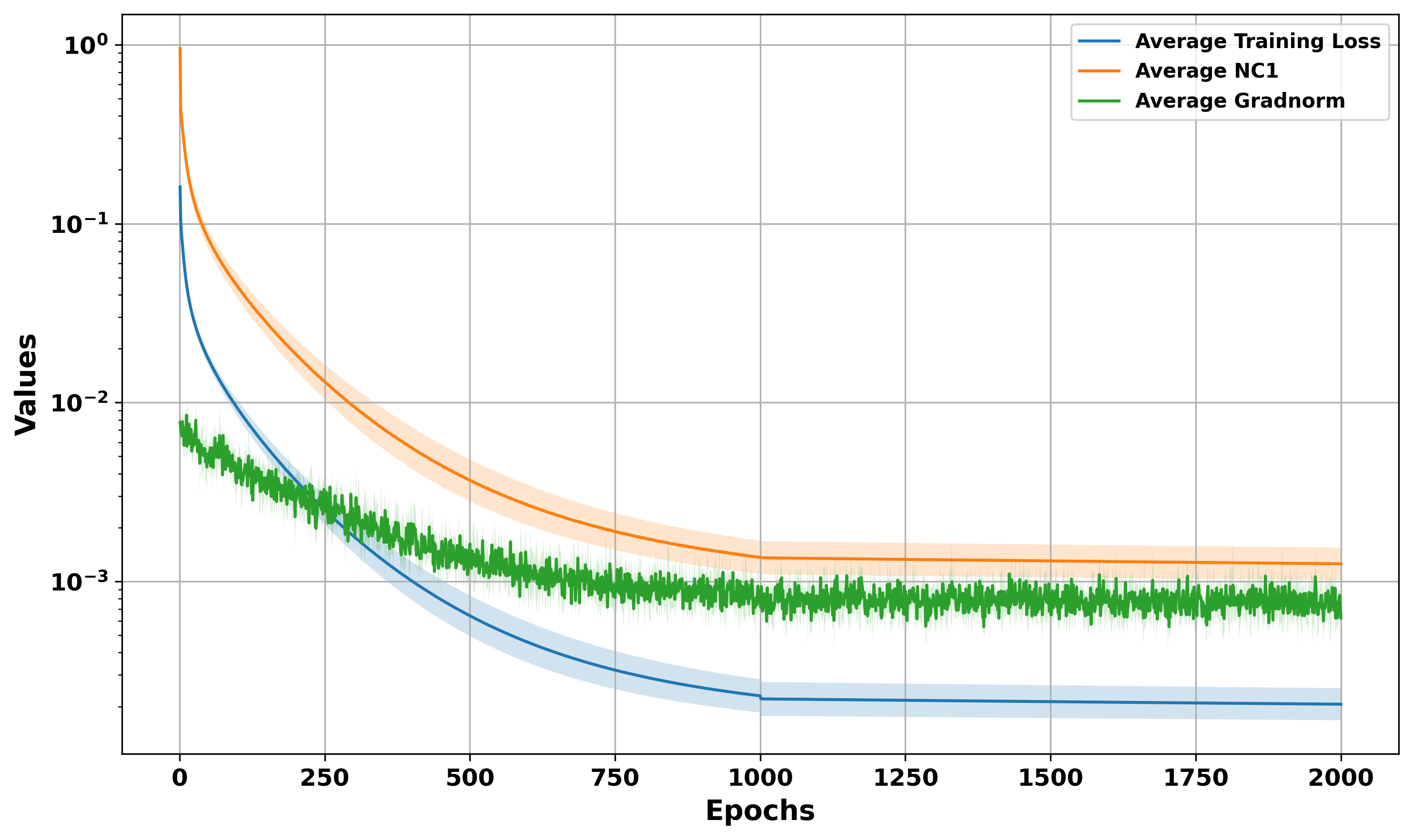
(a)

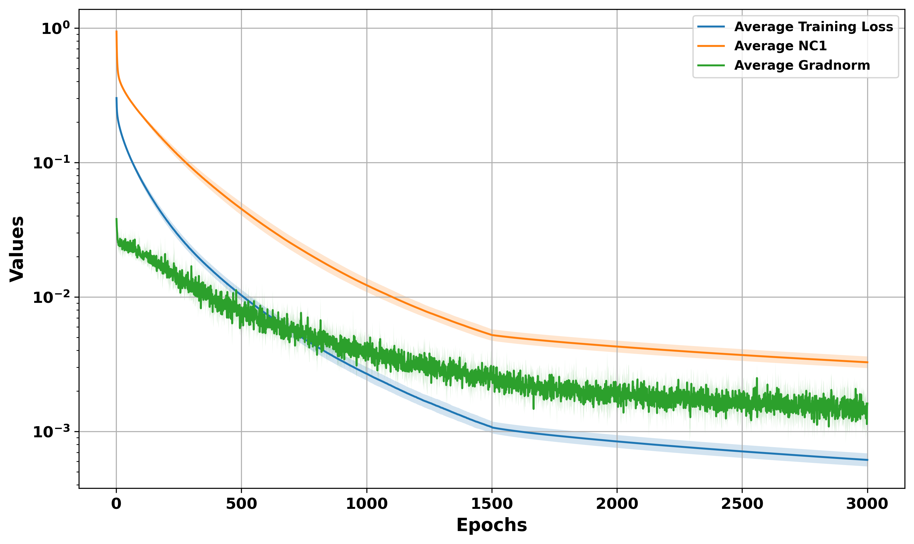
(b)

Figure 1: Average training loss (blue), NC1 (orange) and gradient norm (green) during SGD training. We report the average for 4 independent experiments, as well as the confidence interval at 1 standard deviation.

Imbalancedness after gradient-based training.

The numerical results of Figure 1 show that, even if the solution obtained via gradient descent is not balanced, its training loss and gradient norm are still small and, therefore, as predicted by our analysis, it satisfies NC1. As a normalized balancedness measure, we use:

$$\begin{split}&NB(\rho,W)=\|\mathbb{E}_{\rho}[aa^{\top}]-c_{*}WW^{\top}\|_{op}/\|\mathbb{E}_{\rho}[aa^{\top}]\|_{op},\end{split}$$ (25)

with

$$\begin{split}&c_{*}=\operatorname*{arg\,min}_{c}\|\mathbb{E}_{\rho}[aa^{\top}]-cWW^{\top}\|_{F}^{2},\end{split}$$ (26)

which captures the extent to which $\mathbb{E}_{\rho}[aa^{\top}]$ and $WW^{\top}$ are proportional. We then train the three-layer neural network $f_{N}(x)=W^{\top}h_{N}(x)$, with $h_{N}(x)$ given by (2), and consider the following two settings.

Setting (a): MNIST. We relabel the dataset into $q=3$ classes taking the original label modulo $3$, and we randomly pick $10000$ samples in each new class for training. The input dimension is $d=784$, the number of neurons in the first layer is $N=6272$, and the number of neurons in the second one is $p=16$. We train the model with SGD of batch size $64$ and learning rate $\eta\in\{0.001,0.01\}$, using the smaller (larger) learning rate for the first (second) half of the epochs. We pick weight decay $\lambda_{W}=\lambda_{\rho}=10^{-4}$, but add no noise ($\beta^{-1}=0$) and fix the last linear layer at initialization, which produces an imbalanced network. In fact, at convergence, $NB(\rho,W)=\{0.8093,0.7149,0.5895,0.8531\}$ in our $4$ independent experiments. We also plot the evolution of the normalized balancedness metric in (25) as a function of the number of training epochs in Figure 2(a) of Appendix E, which shows that the network does not achieve balancedness throughout training. However, even if the network is not balanced, Figure 1(a) still shows that the NC1 metric decreases and flattens to a rather low value, following the same pattern as the training loss and the gradient norm.

Setting (b): CIFAR-100. We perform classification on super-classes using pretrained ResNet50 features. Specifically, we consider the $3$ super-classes ["aquatic mammals", "large carnivores", "people"], with each super-class containing $5$ original classes and $500$ samples in total. We then take a ResNet50 pretrained on ImageNet-1K, extract the penultimate-layer features of the training set, and use the such features as training data. The input dimension is $d=2048$, the number of neurons in the first layer is $N=16384$, and the number of neurons in the second one is $p=64$. We train the model with noisy SGD of batch size $64$, pick weight decay $\lambda_{W}=\lambda_{\rho}=\beta=10^{-4}$ and learning rate $\eta\in\{0.001,0.0001\}$, using the smaller (larger) learning rate for the first (second) half of the epochs. As in the previous case, the network does not achieve balancedness throughout training: at convergence, $NB(\rho,W)=\{0.5386,0.2779,0.4141,0.5257\}$ in the $4$ independent experiments; see also Figure 2(b) in Appendix E for a plot of the metric in (25) as a function of the number of training epochs. Nevertheless, the NC1 metric decreases with the loss and the gradient norm, reaching a small value at the end of training, see Figure 1(b).

5 Within-class variability collapse and generalization

While neural collapse is widely known as a phenomenon occurring at training time, it does not necessarily imply that the test error is small (Hui et al.,, 2022, Section 4). We now show that, for well-separated datasets, training via gradient flow implies both approximate NC1 and small test error.

Problem setting.

We make the following additional assumptions (consistent with Assumption 1).

Assumption 3.

We set $\gamma=1$, and assume the activation function $\sigma$ to be the sigmoid function, i.e., $\sigma(z)=\frac{1}{1+e^{-z}}.$ We further assume there are $q$ classes and $n$ data points $(x_{j},y_{j})$ sampled i.i.d. from $\mathcal{D}$, with $m$ points for each class and $x_{j}\sim\mathcal{D}(x_{j}|y_{j})$. Each class is balanced, in the sense that $\int\mathcal{D}(\cdot,e_{k})=1/q$ for all $k$.

For technical reasons, we consider the approximated model obtained by truncating the second layer, i.e., $h^{R}_{\rho}(x)=\mathbb{E}_{\rho}[\tau_{R}(a)\sigma(u^{\top}x)]$, where $\tau_{R}:\mathbb{R}\rightarrow\mathbb{R}$ is a smooth function applied component-wise such that

$$\tau_{R}(z)=\begin{cases}z,&\text{ for $|z|\leq R$, }\\ R+C_{0},&\text{ for $|z|\geq 2R$, }\\ \text{smooth interpolation},&\text{ for $R<|z|<2R$. }\end{cases}$$

Notably, for large enough $R$, the derivative of $\tau$ satisfies

$$\tau^{\prime}_{R}(z)=\begin{cases}1,&\text{ for $|z|\leq R$, }\\ 0,&\text{ for $|z|\geq 2R$, }\\ \leq C_{0},&\text{ for $R<|z|<2R$. }\end{cases}$$

We also denote $H^{R}_{\rho}=[h^{R}_{\rho}(x_{1}),\dots,h^{R}_{\rho}(x_{n})]\in\mathbb{R}^{p\times n}$, and define the loss and free energy w.r.t. the approximated second layer as

$$\begin{split}\mathcal{L}_{n}^{R}(\rho,W)&=\frac{1}{2n}\|W^{\top}H_{\rho}^{R}-Y\|_{F}^{2},\\ \mathcal{E}_{n}^{R}(\rho,W;\beta)&=\mathcal{L}^{R}_{n}(\rho,W)+\frac{\beta^{-1}}{2}\|W\|_{F}^{2}+\frac{\beta^{-1}}{2}\mathbb{E}_{\rho}[\|\theta\|_{2}^{2}]+\beta^{-1}\mathbb{E}_{\rho}[\log\rho].\end{split}$$

Two stage training algorithm.

Our result holds for the two-stage training described in Algorithm 1.

 Initialization: Let $W_{0}=[e_{1},\dots,e_{q}]^{\top}$.

 Stage 1: Fix $W_{0}$ and obtain $\rho_{1}=\operatorname*{arg\,min}_{\rho}\mathcal{E}_{n}^{R}(\rho,W_{0})$.

 Stage 2: Initialize at $(W_{0},\rho_{1})$ and run the following Wasserstein gradient flow:

$$\begin{split}&\differential W_{t}=-\nabla_{W}\mathcal{L}_{\lambda,n}(\rho_{t},W_{t})\differential t;\\ &\differential\theta_{t}=-\nabla_{\theta}\frac{\delta}{\delta\rho}\mathcal{L}_{\lambda,n}(\rho_{t},W_{t})(\theta_{t})\differential t+\sqrt{2\beta^{-1}}\differential B_{t}.\end{split}$$

Algorithm 1 Two-stage gradient flow

Specifically, in Stage 1, we aim to find the global optimum of $\mathcal{E}_{n}^{R}(W_{0},\rho)$ having fixed $W_{0}$, and in Proposition 5.1 below we show that, for all fixed non-zero $W_{0}$, $\mathcal{E}_{n}^{R}(W_{0},\rho)$ has a unique global minimizer in $\mathscr{P}_{2}(\mathbb{R}^{p+d}).$ Furthermore, such global minimizer is achieved by noisy gradient flow as studied by Suzuki et al., 2024a . In Stage 2, we run a gradient flow on the free energy, as we did in Section 4.2.

Proposition 5.1.

Under Assumption 1, for any fixed non-zero $W$, $\mathcal{E}_{n}^{R}(\rho,W)$ is strongly convex in $\rho$, and there exist a unique global minimizer $\rho$ with the following Gibbs form:

$$\begin{split}\rho(\theta)\propto&\exp\left(-\frac{\beta}{n}\tau_{R}(a)^{\top}W(W^{\top}H_{\rho}^{R}-Y)\sigma(X^{\top}u)-\frac{\beta}{2}\|\theta\|_{2}^{2}\right).\end{split}$$ (27)

Proof.

The result follows from the strong convexity of $\mathcal{E}_{n}^{R}(\rho,W)$. In fact, $\frac{1}{2n}\|W^{\top}H_{\rho}^{R}-Y\|_{F}^{2}$ is convex in $H_{\rho}^{R}$, $H_{\rho}^{R}$ is linear in $\rho$, the $L^{2}$-regularization is convex and the entropic regularization is strongly convex. Then, the claim is a consequence of  (Hu et al.,, 2021, Proposition 2.5). ∎

Test error analysis.

We start by introducing $(\tau,M)$-linearly separable data, which intuitively corresponds to each class being linearly separable w.r.t. the others.

Definition 5.2.

We say that the data distribution $\mathcal{D}$ of a $q$-class classification problem is bounded and $(\tau,M)$-linearly separable if, for each $k$, there exist $\hat{u}_{k}$ s.t. $\|\hat{u}_{k}\|^{2}_{2}\leq M^{2}$ and

$$\hat{u}_{k}^{\top}x\begin{cases}&\geq\tau,\hskip 5.69054pt\text{if $x\in\text{supp}(\mathcal{D}(\cdot|e_{k}))$},\\ &<-\tau\hskip 5.69054pt\text{if $x\in\text{supp}(\mathcal{D}(\cdot|e_{k^{\prime}}))$, for all $k^{\prime}\neq k$}.\end{cases}$$

Given a predictor $f:\mathbb{R}^{d}\xrightarrow{}\mathbb{R}^{q}$, we aim to bound the mismatch error:

$$\textbf{err}_{\text{test}}(f;\mathcal{D})=\frac{1}{q}\sum_{k=1}^{q}\Pr_{x\sim\mathcal{D}(\cdot|e_{k})}[\text{One-Hot}(f(x))\neq e_{k}],$$

where we define the function $\text{One-Hot}:\mathbb{R}^{q}\xrightarrow{}\mathbb{R}^{q}$ as $[\text{One-Hot}(f)]_{i}=\begin{cases}1,\hskip 5.69054pt\text{if $i=\operatorname*{arg\,max}_{i}[f]_{i}$},\\ 0,\hskip 5.69054pt\text{else}.\end{cases}$

We now show that training on a $(\tau,M)$-linearly separable dataset leads to both neural collapse and test error vanishing in the number of training samples $n.$

Theorem 5.3.

Under Assumptions 1 and 3, let the data distribution be bounded and $(\tau,M)$-linear separable as per Definition 5.2. Pick $R>1$ large enough, $n$ large enough, and $\beta=\left(640C_{1}^{2}nC_{9}^{2}\frac{1}{\delta_{0}}\right)^{6}$. Then, for any $(\rho_{t},W_{t})$ obtained by Stage 2 of Algorithm 1, we have

$$\begin{split}\textbf{err}_{test}(f(\cdot;\rho_{t},W_{t});\mathcal{D})&\leq C_{10}\log(C_{11}n/\delta_{0})\sqrt{\frac{1}{2n}}+6q\sqrt{\frac{\log(2/\delta)}{n}},\end{split}$$

with probability at least $1-\delta.$ Furthermore, there exists $T(\beta)$ s.t. for all $t>T(\beta)$ except a finite Lebesgue measure set,

$$NC1(H_{\rho_{t}})\leq\delta_{0}.$$

The constants $C_{9},C_{10},C_{11}$ depend on $d,p,C_{0},C_{1},M,\tau,$ but not on $n.$ Their expression is provided in Theorem D.6, whose statement and proof are in Appendix D.1. The argument uses Rademacher complexity bounds for neural networks in the mean-field regime as in (Chen et al.,, 2020; Suzuki et al., 2024b, ; Takakura and Suzuki,, 2024), and the key component is to control the dependence of the constant $C_{10}$ on $n$. This is achieved by noting that, for a $(\tau,M)$-separated data distribution, a two-layer network with constant number of neurons approximately interpolates the data.

In a nutshell, Theorem 5.3 provides a sufficient condition on the data distribution to achieve both NC1 and vanishing test error. Although for simplicity in the statement we pick a specific value for $\beta$, we note that a similar result would hold for $\left(640C_{1}^{2}nC_{9}^{2}\frac{1}{\delta_{0}}\right)^{6}\leq\beta\leq\mathcal{O}(\text{poly}(n))$.

6 Conclusions

In this work, we consider a three-layer neural network in the mean-field regime and give rather general sufficient conditions for within-class variability collapse (namely, NC1) to occur. We then show that (i) training the three-layer neural network with gradient flow satisfies these conditions, and (ii) a vanishing test error is compatible with neural collapse at training time. Taken together, our results connect representation geometry to loss landscape, gradient flow dynamics and generalization, offering new insights into gradient-based optimization in deep learning.

Two interesting future directions include (i) establishing more general conditions (either necessary or sufficient) that guarantee both neural collapse during training and vanishing test error, and (ii) tackling the challenging case in which there is a non-linearity between the last two layers – a setting where the properties of neural collapse have been proved in the UFM framework for binary classification (Súkeník et al.,, 2023).

Appendix A Technical lemmas

Lemma A.1 (Properties of Kronecker product and vectorization).

The following properties hold:

1. $vec(ABC)=(C^{\top}\otimes A)vec(B)$.

2. $(A\otimes B)(C\otimes D)=(AC)\otimes(BD)$ if one can form matrix product $AC$ and $BD$.

3. Singular space of Kronecker product: given two matrices $A\in\mathbb{R}^{m\times n}$ and $B\in\mathbb{R}^{p\times q}$, let their SVD be

   $$A=U_{A}S_{A}V_{A}^{\top},\quad B=U_{B}S_{B}V_{B}^{\top},$$

   where $U_{A}\in\mathbb{R}^{m\times m},S_{A}\in\mathbb{R}^{m\times n},V_{A}\in\mathbb{R}^{n\times n}$ and $U_{B}\in\mathbb{R}^{p\times p},S_{B}\in\mathbb{R}^{p\times q},V_{B}\in\mathbb{R}^{q\times q}$. Then, the SVD of $A\otimes B$ reads

   $$A\otimes B=(U_{A}\otimes U_{B})(S_{A}\otimes S_{B})(V_{A}\otimes V_{B})^{\top}.$$

Proof.

The first two claims can be easily verified. For the third, we have:

$$\begin{split}(U_{A}\otimes U_{B})(S_{A}\otimes S_{B})(V_{A}\otimes V_{B})^{\top}&=(U_{A}\otimes U_{B})(S_{A}\otimes S_{B})(V_{A}^{\top}\otimes V_{B}^{\top})\\ &=(U_{A}\otimes U_{B})((S_{A}V_{A}^{\top})\otimes(S_{B}V_{B}^{\top}))\\ &=((U_{A}S_{A}V_{A}^{\top})\otimes(U_{B}S_{B}V_{B}^{\top}))\\ &=A\otimes B,\end{split}$$

and

$$(U_{A}\otimes U_{B})^{\top}(U_{A}\otimes U_{B})=(U_{A}^{\top}U_{A})\otimes(U_{B}^{\top}U_{B})=I_{m}\otimes I_{p}=I_{mp},$$

which gives the desired result. ∎

Lemma A.2.

Given two matrix $A,B\in\mathbb{R}^{n\times n}$, assume that $A$ is invertible and $A+B$ is invertible , then we have:

$$(A+B)^{-1}=A^{-1}-(A+B)^{-1}BA^{-1}.$$

Proof.

Let $(A+B)^{-1}=A^{-1}+C$ where we aim to compute $C$. Then, we have $(A+B)A^{-1}+(A+B)C=I$. This implies that $BA^{-1}+(A+B)C=0$, and we have $C=-(A+B)^{-1}BA^{-1}$, which gives the desired result. ∎

Lemma A.3.

Let $\rho(\theta)\in\mathscr{P}_{2}(\mathbb{R}^{D})$ be an absolutely continuous measure, $\mathcal{L}(\rho):\mathscr{P}_{2}\xrightarrow{}\mathbb{R}$ be a non-negative functional, and

$$\mathcal{E}(\rho)=\mathcal{L}(\rho)+\frac{\lambda}{2}\mathbb{E}_{\rho}[\|\theta\|_{2}^{2}]+\beta^{-1}\mathbb{E}_{\rho}[\log\rho].$$

Then, for any $\rho\in\mathscr{P}_{2}(\mathbb{R}^{D})$, we have that

$$\begin{split}&\mathcal{L}(\rho)\leq\mathcal{E}(\rho)+\beta^{-1}\frac{D}{2}\log\frac{2\pi}{\lambda\beta},\\ &D_{KL}(\rho||\rho_{0})\leq\beta\left(\mathcal{E}(\rho)+\beta^{-1}\frac{D}{2}\log\frac{2\pi}{\lambda\beta}\right),\\ &\mathbb{E}_{\rho}[\|\theta\|_{2}^{2}]\leq 4\lambda^{-1}\mathcal{E}(\rho)+4\lambda^{-1}\beta^{-1}\left(1+D\log\frac{8\pi}{\lambda\beta}\right),\\ &\mathcal{L}(\rho)+\frac{\lambda}{2}\mathbb{E}_{\rho}[\|\theta\|_{2}^{2}]\leq 3\mathcal{E}(\rho)+\beta^{-1}\frac{D}{2}\log\frac{2\pi}{\lambda\beta}+2\beta^{-1}\left(1+D\log\frac{8\pi}{\lambda\beta}\right),\end{split}$$

where $\rho_{0}\propto\exp(-\beta\lambda\|\theta\|_{2}^{2}/2)$.

Proof.

Note that

$$\beta^{-1}\frac{\beta\lambda}{2}\mathbb{E}_{\rho}[\|\theta\|_{2}^{2}]+\beta^{-1}\mathbb{E}_{\rho}[\log\rho]= \beta^{-1}\mathbb{E}_{\rho}\left[\log\frac{\rho}{(2\pi/(\beta\lambda))^{-D/2}\exp(-\beta\lambda\|\theta\|_{2}^{2}/2)}\right]-\beta^{-1}\frac{D}{2}\log\frac{2\pi}{\beta\lambda}$$

$$\geq -\beta^{-1}\frac{D}{2}\log\frac{2\pi}{\lambda\beta},$$

where the last passage follows from the non-negativity of the KL divergence. This implies that

$$\mathcal{E}(\rho)=\mathcal{L}(\rho)+\beta^{-1}D_{KL}(\rho||\rho_{0})-\beta^{-1}\frac{D}{2}\log\frac{2\pi}{\lambda\beta}\geq\mathcal{L}(\rho)-\beta^{-1}\frac{D}{2}\log\frac{2\pi}{\lambda\beta},$$

which gives the first two inequalities. The third inequality on the second moment follows from (Mei et al.,, 2018, Equation 10.12), and the final equality comes from combining the first and third inequality. ∎

Appendix B Proofs for Section 4.1

B.1 Proof of Theorem 4.2

First, given $\rho,W$, we define

$$\Delta_{a}(\theta;\rho,W):=\nabla_{a}\frac{\delta}{\delta\rho}\mathcal{E}_{n}(\rho,W)(\theta)=\frac{\gamma}{n}W(\gamma W^{\top}H_{\rho}-Y)\sigma(X^{\top}u)+\lambda_{\rho}a+\beta^{-1}\nabla_{a}\log\rho(\theta),\hskip 5.69054pt\rho\hskip 5.69054pta.s.$$ (28)

and we will use the shorthand $\Delta_{a}$ in the rest of the proof. By the definition of ${\epsilon}_{S}$-stationary point, we have

$$\mathbb{E}_{\rho}[\|\Delta_{a}\|_{2}^{2}]\leq{\epsilon}_{S}^{2}.$$

By rearranging terms in (28), we have

$$a=-\frac{\gamma\lambda_{\rho}^{-1}}{n}W(\gamma W^{\top}H_{\rho}-Y)\sigma(X^{\top}u)-\lambda_{\rho}^{-1}\beta^{-1}\nabla_{a}\log\rho(\theta)+\lambda_{\rho}^{-1}\Delta_{a},\hskip 5.69054pt\rho\hskip 5.69054pta.s.$$

which implies that

$$\begin{split}H_{\rho}&=\mathbb{E}_{\rho}[a\sigma(u^{\top}X)]\\ &=-\lambda_{\rho}^{-1}\gamma W(\gamma W^{\top}H_{\rho}-Y)\frac{K_{\rho}(X,X)}{n}-\lambda_{\rho}^{-1}\beta^{-1}\mathbb{E}_{\rho}[\nabla_{a}\log\rho(\theta)\sigma(u^{\top}X)]+\lambda_{\rho}^{-1}\mathbb{E}_{\rho}[\Delta_{a}\sigma(u^{\top}X)].\end{split}$$

We first show that the term $\mathbb{E}_{\rho}[\nabla_{a}\log\rho(\theta)\sigma(u^{\top}x)]=0,$ for any $x$. To see this, it is sufficient to show that

$$\int\partial_{a_{1}}\log\rho(\theta)\sigma(u^{\top}x)\,\rho(\differential\theta)=0.$$

Indeed, we have

$$\begin{split}\int\partial_{a_{1}}\log\rho(\theta)\sigma(u^{\top}x)\,\rho(\differential\theta)&=\int\partial_{a_{1}}\rho(\theta)\sigma(u^{\top}x)\,\differential\theta=-\int\partial_{a_{1}}\sigma(u^{\top}x)\,\rho(\differential\theta)=0,\end{split}$$

which implies that

$$\begin{split}H_{\rho}&=-\lambda_{\rho}^{-1}\gamma W(\gamma W^{\top}H_{\rho}-Y)\frac{K_{\rho}(X,X)}{n}+\lambda_{\rho}^{-1}\mathbb{E}_{\rho}[\Delta_{a}\sigma(u^{\top}X)].\end{split}$$ (29)

By multiplying both sides of (29) with $\gamma W^{\top}$ and subtracting $Y$, we get

$$\gamma W^{\top}H_{\rho}-Y=-\lambda_{\rho}^{-1}\gamma^{2}W^{\top}W(\gamma W^{\top}H_{\rho}-Y)\frac{K_{\rho}(X,X)}{n}+\lambda_{\rho}^{-1}\gamma W^{\top}\mathbb{E}_{\rho}[\Delta_{a}\sigma(u^{\top}X)]-Y.$$

An application of the first property stated in Lemma A.1 gives that

$$vec(\gamma W^{\top}H_{\rho}-Y)=-\lambda_{\rho}\left(\gamma^{2}\frac{K_{\rho}(X,X)}{n}\otimes(W^{\top}W)+\lambda_{\rho}I_{nq}\right)^{-1}\left(vec(Y)-\lambda_{\rho}^{-1}vec(\gamma W^{\top}\mathbb{E}_{\rho}[\Delta_{a}\sigma(u^{\top}X)])\right).$$ (30)

Plugging the expression for $vec(\gamma W^{\top}H_{\rho}-Y)$ back to (29), we have

$$\begin{split}vec(H_{\rho})&=-\lambda_{\rho}^{-1}\left(\gamma\frac{K_{\rho}(X,X)}{n}\otimes W\right)vec(\gamma W^{\top}H_{\rho}-Y)+\lambda_{\rho}^{-1}vec(\mathbb{E}_{\rho}[\Delta_{a}\sigma(u^{\top}X)])\\ &=\left(\gamma\frac{K_{\rho}(X,X)}{n}\otimes W\right)\left(\gamma^{2}\frac{K_{\rho}(X,X)}{n}\otimes(W^{\top}W)+\lambda_{\rho}I_{nq}\right)^{-1}\left(vec(Y)-\lambda_{\rho}^{-1}vec(W^{\top}\mathbb{E}_{\rho}[\Delta_{a}\sigma(u^{\top}X)])\right)\\ &\quad+\lambda_{\rho}^{-1}vec(\mathbb{E}_{\rho}[\Delta_{a}\sigma(u^{\top}X)])\\ &=\left(\gamma\frac{K_{\rho}(X,X)}{n}\otimes W\right)\left(\gamma^{2}\frac{K_{\rho}(X,X)}{n}\otimes(W^{\top}W)+\lambda_{\rho}I_{nq}\right)^{-1}vec(Y)+{\bm{E}}_{1}({\epsilon}_{S},\lambda_{\rho};\gamma,W),\end{split}$$

where we define the error vector as

$$\begin{split}{\bm{E}}_{1}({\epsilon}_{S},\lambda_{\rho};\gamma,W)&=-\lambda_{\rho}^{-1}\left(\gamma\frac{K_{\rho}(X,X)}{n}\otimes W\right)\left(\gamma^{2}\frac{K_{\rho}(X,X)}{n}\otimes(W^{\top}W)+\lambda_{\rho}I_{nq}\right)^{-1}vec(\gamma W^{\top}\mathbb{E}_{\rho}[\Delta_{a}\sigma(u^{\top}X)])\\ &\quad+\lambda_{\rho}^{-1}vec(\mathbb{E}_{\rho}[\Delta_{a}\sigma(u^{\top}X)]).\end{split}$$

Now we aim to upper bound the error. To do so, we write

$$\begin{split}&\|{\bm{E}}_{1}({\epsilon}_{S},\lambda_{\rho};\gamma,W)\|_{2}^{2}\\ &\leq 2\lambda_{\rho}^{-2}\left\|\left(\gamma\frac{K_{\rho}(X,X)}{n}\otimes W\right)\left(\gamma^{2}\frac{K_{\rho}(X,X)}{n}\otimes(W^{\top}W)+\lambda_{\rho}I_{nq}\right)^{-1}vec(\gamma W^{\top}\mathbb{E}_{\rho}[\Delta_{a}\sigma(u^{\top}X)])\right\|_{2}^{2}\\ &\quad+2\lambda_{\rho}^{-2}\|vec(\mathbb{E}_{\rho}[\Delta_{a}\sigma(u^{\top}X)])\|_{2}^{2}\\ &\leq 2\lambda_{\rho}^{-2}\sigma_{\max}\left(\gamma\frac{K_{\rho}(X,X)}{n}\otimes W\right)^{2}\sigma_{\max}\left(\left(\gamma^{2}\frac{K_{\rho}(X,X)}{n}\otimes(W^{\top}W)+\lambda_{\rho}I_{nq}\right)^{-1}\right)^{2}\|\gamma W^{\top}\mathbb{E}_{\rho}[\Delta_{a}\sigma(u^{\top}X)]\|_{F}^{2}\\ &\quad+2\lambda_{\rho}^{-2}\|\mathbb{E}_{\rho}[\Delta_{a}\sigma(u^{\top}X)]\|_{F}^{2}\\ &\leq\left(2\lambda_{\rho}^{-4}\gamma^{4}C_{1}^{2}\sigma_{\max}(W)^{4}+2\lambda_{\rho}^{-2}\right)\|\mathbb{E}_{\rho}[\Delta_{a}\sigma(u^{\top}X)]\|_{F}^{2}.\end{split}$$ (31)

Then, we upper bound $\|\mathbb{E}_{\rho}[\Delta_{a}\sigma(u^{\top}X)]\|_{F}^{2}$ as follows:

$$\begin{split}\|\mathbb{E}_{\rho}[\Delta_{a}\sigma(u^{\top}X)]\|_{F}^{2}&\leq\mathbb{E}_{\rho}[\|\Delta_{a}\sigma(u^{\top}X)\|_{F}^{2}]\\ &=\mathbb{E}_{\rho}[\|\Delta_{a}\|_{2}^{2}\|\sigma(u^{\top}X)\|_{2}^{2}]\\ &\leq C_{1}^{2}n\mathbb{E}_{\rho}[\|\Delta_{a}\|_{2}^{2}]\\ &\leq C_{1}^{2}n{\epsilon}_{S}^{2}.\end{split}$$ (32)

Combining (LABEL:eq:err1) and (32), (6)-(7) readily follow.

To obtain (9), we first show that, when $W^{\top}W$ is full rank, the following equality holds

$$\begin{split}&\left(\gamma\frac{K_{\rho}(X,X)}{n}\otimes W\right)\left(\gamma^{2}\frac{K_{\rho}(X,X)}{n}\otimes W^{\top}W+\lambda_{\rho}I_{nq}\right)^{-1}\\ &\hskip 50.00008pt=\gamma^{-1}(I_{n}\otimes(W(W^{\top}W)^{-1}))-\lambda_{\rho}\gamma^{-1}(I_{n}\otimes(W(W^{\top}W)^{-1}))\left(\frac{K_{\rho}(X,X)}{n}\otimes W^{\top}W+\lambda_{\rho}I_{nq}\right)^{-1}.\end{split}$$ (33)

To do so, define the eigen-decomposition of $\frac{K_{\rho}(X,X)}{n}$ and SVD of $W$ as follows:

$$\frac{K_{\rho}(X,X)}{n}=U_{K}\Sigma_{K}U_{K}^{\top},\quad\gamma W=U_{W}S_{W}V_{W}^{\top},$$

where $U_{K}\in\mathbb{R}^{n\times n},\Sigma_{K}\in\mathbb{R}^{n\times n},U_{W}\in\mathbb{R}^{p\times p},S_{W}\in\mathbb{R}^{p\times q},V_{W}\in\mathbb{R}^{q\times q}$. By Lemma A.1, we have that

$$\gamma\frac{K_{\rho}(X,X)}{n}\otimes W=(U_{K}\otimes U_{W})(\Sigma_{K}\otimes S_{W})(U_{K}\otimes V_{W})^{\top},\quad\gamma^{2}\frac{K_{\rho}(X,X)}{n}\otimes W^{\top}W=(U_{K}\otimes V_{W})(\Sigma_{K}\otimes(S_{W}^{\top}S_{W}))(U_{K}\otimes V_{W})^{\top}.$$

Thus, we have the following equalities:

$$\begin{split}&\left(\gamma\frac{K_{\rho}(X,X)}{n}\otimes W\right)\left(\gamma^{2}\frac{K_{\rho}(X,X)}{n}\otimes W^{\top}W+\lambda_{\rho}I_{nq}\right)^{-1}\\ &=(U_{K}\otimes U_{W})(\Sigma_{K}\otimes S_{W})(U_{K}\otimes V_{W})^{\top}(U_{K}\otimes V_{W})(\Sigma_{K}\otimes(S_{W}^{\top}S_{W})+\lambda_{\rho}I_{nq})^{-1}(U_{K}\otimes V_{W})^{\top}\\ &=(U_{K}\otimes U_{W})(\Sigma_{K}\otimes S_{W})(\Sigma_{K}\otimes(S_{W}^{\top}S_{W})+\lambda_{\rho}I_{nq})^{-1}(U_{K}\otimes V_{W})^{\top}.\end{split}$$

For simplicity, we write the matrix $S_{W}=\begin{bmatrix}diag(\sigma_{1},\dots,\sigma_{q})\\ 0_{p-q,q}\end{bmatrix}$ and define $S^{-1}_{W}=\begin{bmatrix}diag(\sigma^{-1}_{1},\dots,\sigma^{-1}_{q})\\ 0_{p-q,q}\end{bmatrix}$. Here, given integers $n,m$, we define $0_{n,m}$ as the $n\times m$ matrix containing zeros. Clearly, we have that

$$S^{-1}_{W}S_{W}^{\top}=\begin{bmatrix}I_{q}&0_{q,p-q}\\ 0_{p-q,q}&0_{p-q,p-q}\end{bmatrix}.$$

Next, we observe that

$$\begin{split}(I_{n}\otimes S^{-1}_{W}S_{W}^{\top})(\Sigma_{K}\otimes S_{W})=\Sigma_{K}\otimes(S^{-1}_{W}S_{W}^{\top}S_{W})=\Sigma_{K}\otimes S_{W}.\end{split}$$

Thus, we can write

$$\begin{split}(\Sigma_{K}\otimes S_{W})(\Sigma_{K}\otimes(S_{W}^{\top}S_{W})+\lambda_{\rho}I_{nq})^{-1}&=(I_{n}\otimes S^{-1}_{W}S_{W}^{\top})(\Sigma_{K}\otimes S_{W})(\Sigma_{K}\otimes(S_{W}^{\top}S_{W})+\lambda_{\rho}I_{nq})^{-1}\\ &=(I_{n}\otimes S^{-1}_{W})(I_{n}\otimes S_{W}^{\top})(\Sigma_{K}\otimes S_{W})(\Sigma_{K}\otimes(S_{W}^{\top}S_{W})+\lambda_{\rho}I_{nq})^{-1}\\ &=(I_{n}\otimes S^{-1}_{W})(\Sigma_{K}\otimes(S_{W}^{\top}S_{W}))(\Sigma_{K}\otimes(S_{W}^{\top}S_{W})+\lambda_{\rho}I_{nq})^{-1}\\ &=(I_{n}\otimes S^{-1}_{W})\left(I-\lambda_{\rho}(\Sigma_{K}\otimes(S_{W}^{\top}S_{W})+\lambda_{\rho}I_{nq})^{-1}\right),\end{split}$$

which implies that

$$\begin{split}&\left(\gamma\frac{K_{\rho}(X,X)}{n}\otimes W\right)\left(\gamma^{2}\frac{K_{\rho}(X,X)}{n}\otimes W^{\top}W+\lambda_{\rho}I_{nq}\right)^{-1}\\ &=(U_{K}\otimes U_{W})(I_{n}\otimes S_{W}^{-1})(U_{K}\otimes V_{W})^{\top}-\lambda_{\rho}(U_{K}\otimes U_{W})(I_{n}\otimes S_{W}^{-1})(\Sigma_{K}\otimes(S_{W}^{\top}S_{W})+\lambda_{\rho}I_{nq})^{-1}(U_{K}\otimes V_{W})^{\top}.\end{split}$$

Finally, we can verify that:

$$\begin{split}\gamma^{-1}I_{n}\otimes(W(W^{\top}W)^{-1})&=(U_{K}U_{K}^{\top})\otimes(U_{W}S_{W}^{-1}V_{W}^{\top})\\ &=(U_{K}\otimes U_{W})(I_{n}\otimes S_{W}^{-1})(U_{K}\otimes V_{W})^{\top},\end{split}$$

and

$$\begin{split}&\gamma^{-1}(I_{n}\otimes(W(W^{\top}W)^{-1}))\left(\gamma^{2}\frac{K_{\rho}(X,X)}{n}\otimes W^{\top}W+\lambda_{\rho}I_{nq}\right)^{-1}\\ =&(U_{K}\otimes U_{W})(I_{n}\otimes S_{W}^{-1})(U_{K}\otimes V_{W})^{\top}(U_{K}\otimes V_{W})(\Sigma_{K}\otimes(S_{W}^{\top}S_{W})+\lambda_{\rho}I_{nq})^{-1}(U_{K}\otimes V_{W})^{\top}\\ =&(U_{K}\otimes U_{W})(I_{n}\otimes S_{W}^{-1})(\Sigma_{K}\otimes(S_{W}^{\top}S_{W})+\lambda_{\rho}I_{nq})^{-1}(U_{K}\otimes V_{W})^{\top},\end{split}$$

which gives (33).

From the above decomposition, we know that

$$\begin{split}&\left(\gamma\frac{K_{\rho}(X,X)}{n}\otimes W\right)\left(\gamma^{2}\frac{K_{\rho}(X,X)}{n}\otimes W^{\top}W+\lambda_{\rho}I_{nq}\right)^{-1}vec(Y)\\ =&\gamma^{-1}(I_{n}\otimes(W(W^{\top}W)^{-1}))vec(Y)-\lambda_{\rho}\gamma^{-1}(I_{n}\otimes(W(W^{\top}W)^{-1}))\left(\gamma^{2}\frac{K_{\rho}(X,X)}{n}\otimes W^{\top}W+\lambda_{\rho}I_{nq}\right)^{-1}vec(Y)\\ =&\gamma^{-1}vec(W(W^{\top}W)^{-1}Y)-\lambda_{\rho}\gamma^{-1}(I_{n}\otimes(W(W^{\top}W)^{-1}))\left(\gamma^{2}\frac{K_{\rho}(X,X)}{n}\otimes W^{\top}W+\lambda_{\rho}I_{nq}\right)^{-1}vec(Y),\end{split}$$

where we use the first item of Lemma A.1 in the last passage. Let us now define

$$\begin{split}&\widetilde{{\bm{E}}}_{2}({\epsilon}_{S},\lambda_{\rho};\gamma,\rho,W):=-\lambda_{\rho}\gamma^{-1}(I_{n}\otimes(W(W^{\top}W)^{-1}))\left(\gamma^{2}\frac{K_{\rho}(X,X)}{n}\otimes W^{\top}W+\lambda_{\rho}I_{nq}\right)^{-1}vec(Y)\\ =&\gamma^{-1}(I_{n}\otimes(W(W^{\top}W)^{-1}))\left(vec(\gamma W^{\top}H_{\rho}-Y)-\left(\gamma^{2}\frac{K_{\rho}(X,X)}{n}\otimes W^{\top}W+\lambda_{\rho}I_{nq}\right)^{-1}vec\left(\gamma W^{\top}\mathbb{E}_{\rho}[\Delta_{a}\sigma(u^{\top}X)]\right)\right),\end{split}$$

where the second passage follows from (30). Using (6) (that we proved above), we have

$$vec(H_{\rho})=vec(\gamma^{-1}W(W^{\top}W)^{-1}Y)+\widetilde{{\bm{E}}}_{2}({\epsilon}_{S},\lambda_{\rho};\gamma,\rho,W)+{\bm{E}}_{1}({\epsilon}_{S},\lambda_{\rho};\gamma,W).$$

It remains to upper bound $\|\widetilde{{\bm{E}}}_{2}({\epsilon}_{S},\lambda_{\rho};\gamma,\rho,W)\|_{2}^{2}$. To this aim, we write

$$\|\widetilde{{\bm{E}}}_{2}({\epsilon}_{S},\lambda_{\rho};\gamma,\rho,W)\|_{2}^{2} \leq 2\gamma^{-2}\sigma_{\max}(I_{n}\otimes(W(W^{\top}W)^{-1}))^{2}(\|\gamma W^{\top}H_{\rho}-Y\|_{F}^{2}+\lambda_{\rho}^{-2}\gamma^{2}\|W^{\top}\mathbb{E}_{\rho}[\Delta_{a}\sigma(u^{\top}X)]\|_{F}^{2})$$

$$\leq\frac{2n\gamma^{-2}\mathcal{L}_{n}(\rho,W)+2\lambda_{\rho}^{-2}\|W^{\top}\mathbb{E}_{\rho}[\Delta_{a}\sigma(u^{\top}X)]\|_{F}^{2}}{\sigma_{\min}(W)^{2}}$$

$$\leq\frac{2n\gamma^{-2}\mathcal{L}_{n}(\rho,W)+2\lambda_{\rho}^{-2}\sigma_{\max}(W)^{2}\|\mathbb{E}_{\rho}[\Delta_{a}\sigma(u^{\top}X)]\|_{F}^{2}}{\sigma_{\min}(W)^{2}}.$$

Plugging in the bound in (32) gives

$$\|\widetilde{{\bm{E}}}_{2}({\epsilon}_{S},\lambda_{\rho};\gamma,\rho,W)\|_{2}^{2}\leq\frac{2n\gamma^{-2}\mathcal{L}_{n}(\rho,W)+2\lambda_{\rho}^{-2}\sigma_{\max}(W)^{2}C_{1}^{2}n{\epsilon}_{S}^{2}}{\sigma_{\min}(W)^{2}}.$$ (34)

By combining (7) and (34) with an application of the triangle inequality, the proof is complete.

B.2 Proof of Lemma 4.3

Proof of Lemma 4.3.

To upper bound $\sigma_{\max}(W),$ we directly use the definition in (4):

$$\sigma_{\max}(W)^{2}\leq\|W\|_{F}^{2}\leq 2\lambda_{W}^{-1}\mathcal{L}_{\lambda,n}(\rho,W)\leq 2B(\lambda_{W}^{0})^{-1}(\log\beta)^{\alpha}.$$

To lower bound $\sigma_{\min}(W),$ we start by showing that

$$\|H_{\rho}\|^{2}_{F}\leq\beta^{{\epsilon}_{0}}.$$ (35)

To see this, assume by contradiction that $\|H_{\rho}\|^{2}_{F}>\beta^{{\epsilon}_{0}}.$ Then, there exists $i$ such that $\|h_{\rho}(x_{i})\|_{2}^{2}>\frac{\beta^{{\epsilon}_{0}}}{n}$ and the following bounds hold:

$$\|h_{\rho}(x_{i})\|_{2}^{2} =\|\mathbb{E}_{\rho}[a\sigma(u^{\top}x_{i})]\|_{2}^{2}$$

$$=\mathbb{E}_{\theta,\theta^{\prime}}[a^{\top}a^{\prime}\sigma(u^{\top}x_{i})\sigma((u^{\prime})^{\top}x_{i})]\hskip 17.07164pt\text{($\theta^{\prime}$ is an independent copy of $\theta$)}$$

$$\leq\mathbb{E}_{\theta,\theta^{\prime}}[|a|^{\top}|a^{\prime}||\sigma(u^{\top}x_{i})||\sigma((u^{\prime})^{\top}x_{i})|]$$

$$\leq C_{1}^{2}\mathbb{E}_{\theta,\theta^{\prime}}[|a|^{\top}|a|]$$

$$\leq C_{1}^{2}\mathbb{E}_{a}[\|a\|_{2}]\mathbb{E}_{a^{\prime}}[\|a\|_{2}]$$

$$=C_{1}^{2}\mathbb{E}_{a}[\|a\|_{2}]^{2}$$

$$\leq C_{1}^{2}\mathbb{E}_{a}[\|a\|_{2}^{2}],$$

which implies that $\mathbb{E}_{\rho}[\|a\|_{2}^{2}]>\frac{\beta^{{\epsilon}_{0}}}{C_{1}^{2}n}.$ By combining (15) with (4), we have

$$\begin{split}\mathbb{E}_{\rho}[\|a\|_{2}^{2}]\leq\mathbb{E}_{\rho}[\|\theta\|_{2}^{2}]\leq 2B(\lambda_{\rho}^{0})^{-1}(\log\beta)^{\alpha},\end{split}$$ (36)

where we recall that $\lambda_{\rho}=\lambda_{\rho}^{0}\beta^{-1}.$ Note that, for all $\epsilon_{0}\in(0,1)$ and for all $\beta\geq e^{\frac{4\alpha}{\epsilon_{0}}\log\frac{2\alpha}{\epsilon_{0}}}$,

$$\frac{\beta^{\epsilon_{0}}}{(\log\beta)^{\alpha}}\geq\beta^{\epsilon_{0}/2}.$$ (37)

Thus, by taking

$$\beta\geq\max\{e^{\frac{4\alpha}{\epsilon_{0}}\log\frac{2\alpha}{\epsilon_{0}}},(2C_{1}^{2}nB(\lambda_{\rho}^{0})^{-1})^{\frac{2}{{\epsilon}_{0}}}\}$$

as in (14), we have that $\frac{\beta^{{\epsilon}_{0}}}{C_{1}^{2}n}$ is strictly larger than the RHS of (36), which is a contradiction.

Now, we are ready to argue that, for large enough $\beta$, $\sigma_{\min}(W)\geq\beta^{-{\epsilon}_{0}}$. Assume by contradiction that $\sigma_{\min}(W)<\beta^{-{\epsilon}_{0}}$, and w.l.o.g assume $[\Sigma_{W}]_{q,q}<\beta^{-{\epsilon}_{0}}$. Then, the following lower bound holds

$$\begin{split}\mathcal{L}_{\lambda,n}(\rho,W)&\geq\mathcal{L}_{n}(\rho,W)\\ &=\frac{1}{2n}\|W^{\top}H_{\rho}-Y\|_{F}^{2}\\ &=\frac{1}{2n}\|V_{W}\Sigma^{\top}_{W}U_{W}^{\top}H_{\rho}-Y\|_{F}^{2}\\ &=\frac{1}{2n}\|\Sigma^{\top}_{W}U_{W}^{\top}H_{\rho}-V_{W}^{\top}Y\|_{F}^{2}\\ &\geq\frac{1}{2n}\|[\Sigma_{W}]_{q,q}[U_{W}^{\top}H_{\rho}]_{q:}-[V_{W}^{\top}Y]_{q:}\|_{2}^{2}\\ &\geq\frac{1}{4n}\|[V_{W}^{\top}Y]_{q:}\|_{2}^{2}-\frac{1}{2n}\|[\Sigma_{W}]_{q,q}[U_{W}^{\top}H_{\rho}]_{q:}\|_{2}^{2}\\ &=\frac{1}{4q}-\frac{1}{2n}\|[\Sigma_{W}]_{q,q}[U_{W}^{\top}H_{\rho}]_{q:}\|_{2}^{2}\\ &>\frac{1}{4q}-\frac{1}{2n}\beta^{-{\epsilon}_{0}}.\end{split}$$ (38)

Note that by taking $\beta\geq\left(\frac{4q}{n}\right)^{\frac{1}{{\epsilon}_{0}}},$ we have $\frac{1}{4q}-\frac{1}{2n}\beta^{-{\epsilon}_{0}}\geq\frac{1}{8q}.$ Furthermore, for all $\beta\geq e^{4\alpha\log(2\alpha)}$, we have

$$\frac{\beta^{1/\alpha}}{\log\beta}>\beta^{1/(2\alpha)}.$$

Thus, by taking

$$\beta\geq\max\left\{e^{4\alpha\log(2\alpha)},\left(\frac{4q}{n}\right)^{\frac{1}{{\epsilon}_{0}}},64(qB)^{2}\right\},$$

as in (14), we have that the RHS of (38) is strictly larger than $B\beta^{-1}(\log\beta)^{\alpha}$, which is a contradiction and concludes the proof.

∎

B.3 Proof of Corollary 4.4

Proof of Corollary 4.4.

From Theorem 4.2, we have

$$H_{\rho}=\gamma^{-1}W(W^{\top}W)^{-1}Y+{\bm{E}}_{2}.$$

Note that the NC1 metric is scale invariant, thus it is equivalent to compute $NC1(\gamma H_{\rho}).$ Later on, we will write $H_{\rho}:=\gamma H_{\rho}$ with slight abuse of notation. Some manipulations give

$$\begin{split}&\widetilde{H_{\rho}}=W(W^{\top}W)^{-1}\left(Y-\frac{1}{q}\bm{1}_{q}\bm{1}_{n}^{\top}\right)+\gamma{\bm{E}}_{2}\left(I_{n}-\frac{1}{n}\bm{1}_{n}\bm{1}_{n}^{\top}\right),\\ &M_{c}=\frac{1}{m}W(W^{\top}W)^{-1}\left(Y-\frac{1}{q}\bm{1}_{q}\bm{1}_{n}^{\top}\right)Y^{\top}Y+\frac{\gamma}{m}{\bm{E}}_{2}\left(I_{n}-\frac{1}{n}\bm{1}_{n}\bm{1}_{n}^{\top}\right)Y^{\top}Y,\\ &\widetilde{H_{\rho}}-M_{c}=\gamma{\bm{E}}_{2}\left(I_{n}-\frac{1}{n}\bm{1}_{n}\bm{1}_{n}^{\top}\right)\left(I_{n}-\frac{1}{m}Y^{\top}Y\right).\end{split}$$

Thus, we have

$$\begin{split}\Tr{(\widetilde{H_{\rho}}-M_{c})^{\top}(\widetilde{H_{\rho}}-M_{c})}&=\|\widetilde{H_{\rho}}-M_{c}\|_{F}^{2}\\ &=\left\|\gamma{\bm{E}}_{2}\left(I_{n}-\frac{1}{n}\bm{1}_{n}\bm{1}_{n}^{\top}\right)\left(I_{n}-\frac{1}{m}Y^{\top}Y\right)\right\|_{F}^{2}\\ &\leq 16\gamma^{2}\|{\bm{E}}_{2}\|_{F}^{2},\\ \Tr{\widetilde{H_{\rho}}^{\top}\widetilde{H_{\rho}}}&=\|\widetilde{H_{\rho}}\|_{F}^{2}\\ &\geq\frac{1}{2}\left\|W(W^{\top}W)^{-1}\left(Y-\frac{1}{q}\bm{1}_{q}\bm{1}_{n}^{\top}\right)\right\|_{F}^{2}-\|\gamma{\bm{E}}_{2}\left(I_{n}-\frac{1}{n}\bm{1}_{n}\bm{1}_{n}^{\top}\right)\|_{F}^{2}\\ &\geq\frac{1}{2\sigma_{\max}^{2}(W)}\frac{(q-1)n}{q}-4\gamma^{2}\|{\bm{E}}_{2}\|_{F}^{2},\end{split}$$

which concludes the proof. ∎

B.4 Proof of Lemma 4.5

Proof of Lemma 4.5.

From the stationary condition, we obtain

$$\begin{split}&\nabla_{a}\frac{\delta}{\delta\rho}\mathcal{E}_{n}(\rho,W)=\frac{\gamma}{n}W(\gamma W^{\top}H_{\rho}-Y)\sigma(X^{\top}u)+\lambda_{\rho}a+\beta^{-1}\nabla_{a}\log\rho(\theta)=0,\quad\rho\hskip 5.69054pta.s.\\ &\nabla_{W}\mathcal{E}_{n}(\rho,W)=\frac{\gamma}{n}H_{\rho}(\gamma W^{\top}H_{\rho}-Y)^{\top}+\lambda_{W}W=0.\end{split}$$

Rearranging the terms gives

$$\begin{split}&a=-\frac{\lambda_{\rho}^{-1}\gamma}{n}W(\gamma W^{\top}H_{\rho}-Y)\sigma(X^{\top}u)-\beta^{-1}\lambda_{\rho}^{-1}\nabla_{a}\log\rho(\theta),\quad\rho\hskip 5.69054pta.s.\\ &W=-\frac{\lambda_{W}^{-1}\gamma}{n}H_{\rho}(\gamma W^{\top}H_{\rho}-Y)^{\top}.\end{split}$$

Then, we compute:

$$\begin{split}\mathbb{E}_{\rho}[aa^{\top}]&=\mathbb{E}_{\rho}\left[-\frac{\lambda_{\rho}^{-1}\gamma}{n}W(\gamma W^{\top}H_{\rho}-Y)\sigma(X^{\top}u)a^{\top}-\beta^{-1}\lambda_{\rho}^{-1}(\nabla_{a}\log\rho(\theta))a^{\top}\right],\\ &=-\frac{\lambda_{\rho}^{-1}\gamma}{n}W(\gamma W^{\top}H_{\rho}-Y)H_{\rho}^{\top}-\beta^{-1}\lambda_{\rho}^{-1}\mathbb{E}_{\rho}\left[(\nabla_{a}\log\rho(\theta))a^{\top}\right]\\ WW^{\top}&=-\frac{\lambda_{W}^{-1}\gamma}{n}W(\gamma W^{\top}H_{\rho}-Y)H_{\rho}^{\top}.\end{split}$$

Thus, $\lambda_{W}WW^{\top}-\lambda_{\rho}\mathbb{E}_{\rho}[aa^{\top}]=\beta^{-1}\mathbb{E}_{\rho}\left[(\nabla_{a}\log\rho(\theta))a^{\top}\right]$, and next we compute $\mathbb{E}_{\rho}\left[(\nabla_{a}\log\rho(\theta))a^{\top}\right].$ To do this, we note that:

$$\begin{split}\left[\mathbb{E}_{\rho}\left[(\nabla_{a}\log\rho(\theta))a^{\top}\right]\right]_{i,j}&=\mathbb{E}_{\rho}\left[\partial_{a_{i}}\log\rho(\theta)a_{j}\right]\\ &=\int\rho(\theta)\partial_{a_{i}}\log\rho(\theta)a_{j}\,\differential\theta\\ &=\int a_{j}\partial_{a_{i}}\rho(\theta)\,\differential\theta\\ &=-\int\rho(\theta)\partial_{a_{i}}a_{j}\,\differential\theta\\ &=\begin{cases}&-1,\quad i=j\\ &0,\quad i\neq j\end{cases}\end{split}$$

Thus, $\mathbb{E}_{\rho}\left[(\nabla_{a}\log\rho(\theta))a^{\top}\right]=-I_{p},$ which gives the desired result. ∎

Appendix C Proofs in Section 4.2

C.1 Proof of Lemma 4.6

Proof of Lemma 4.6 .

We note that $\mathcal{E}_{n}(\rho,W)$ is lower bounded and we have:

$$\mathcal{E}_{n}(\rho_{T},W_{T})=\mathcal{E}_{n}(\rho_{0},W_{0})+\int_{0}^{T}\partial_{t}\mathcal{E}_{n}(\rho_{t},W_{t})\,\differential t.$$

A standard computation gives

$$\partial_{t}\mathcal{E}_{n}(\rho_{t},W_{t})=-\mathbb{E}_{\rho_{t}}\left[\left\|\nabla_{\theta}\frac{\delta}{\delta\rho}\mathcal{E}_{n}(\rho_{t},W_{t})(\theta_{t})\right\|_{2}^{2}\right]-\|\nabla_{W}\mathcal{L}_{\lambda,n}(\rho_{t},W_{t})\|_{2}^{2},$$

which implies that $\mathcal{E}_{n}(\rho_{T},W_{T})$ is a lower-bounded monotone decreasing sequence. Thus, $\lim_{T\rightarrow\infty}\mathcal{E}_{n}(\rho_{T},W_{T})=C<\infty.$ The existence and boundedness of $\lim_{T\rightarrow\infty}\mathcal{E}_{n}(\rho_{T},W_{T})$ implies that, for any ${\epsilon}_{S}>0,$ there exists $T({\epsilon}_{S})>0$ s.t. for all $t>T({\epsilon}_{S})$ except a finite Lebesgue measure set,

$$\mathbb{E}_{\rho_{t}}\left[\left\|\nabla_{\theta}\frac{\delta}{\delta\rho}\mathcal{E}_{n}(\rho_{t},W_{t})(\theta_{t})\right\|_{2}^{2}\right]+\|\nabla_{W}\mathcal{E}_{n}(\rho_{t},W_{t})\|_{2}^{2}\leq{\epsilon}_{S},$$

which finishes the proof. ∎

C.2 Proof of Theorem 4.8.

Theorem C.1 (Full statement of Theorem 4.8).

Let Assumptions 1, 2 hold, set $\lambda_{\rho}=\lambda_{W}=\beta^{-1}$ and

$$\gamma>C_{3},\quad t_{0}=\beta C_{5}.$$

Then, for any $\beta$ and any $t\geq t_{0}$, we have

$$\mathcal{L}_{\lambda,n}(\rho_{t},W_{t})\leq\beta^{-1}C_{4},$$

where

$$\begin{split}&C_{3}=\max\left\{\frac{4B_{1}}{R_{W}},\frac{2\sqrt{2}B_{3}}{\sqrt{R_{\rho}}}\right\},\\ &C_{4}=6\gamma^{-2}A_{1}^{2}\max\left\{\frac{B_{2}^{2}}{B_{1}^{2}},\frac{B_{4}^{2}}{B_{3}^{2}}\right\}+6\gamma^{-2}A_{2}^{2}+3\frac{q(R_{W}+1)}{2}+3R_{\rho}+\frac{p+d}{2}\log 2\pi+2\left(1+(p+d)\log 8\pi\right),\\ &C_{5}=\gamma^{-1}\min\left\{\frac{B_{1}}{B_{2}},\frac{B_{3}}{B_{4}}\right\},\\ &R_{W}=\frac{1}{2},\quad R_{\rho}=\min\left\{p+d,\frac{\lambda_{*}^{2}}{64n^{2}C_{1}^{2}}\right\},\\ &A_{1}=\frac{\lambda_{*}}{2n},\quad A_{2}=32\frac{\sqrt{2n(R_{W}+1)R_{\rho}}(2C_{1}d\sqrt{p+d}+1)}{\lambda_{*}},\\ &B_{1}=\frac{2}{n}\sqrt{R_{W}+1}\sqrt{pn}(4C_{1}\sqrt{d(p+d)}+2C_{1})2\sqrt{R_{\rho}}A_{1}^{-1},\\ &B_{2}=2(R_{W}+1)+\frac{2}{n}\sqrt{R_{W}+1}\sqrt{pn}(4C_{1}\sqrt{d(p+d)}+2C_{1})2\sqrt{R_{\rho}}A_{2},\\ &B_{3}=2p\sqrt{n}\sqrt{R_{W}+1}(4C_{1}\sqrt{d(p+d)}+2C_{1})2\sqrt{R_{\rho}}(4C_{1}d^{3/2}\sqrt{p+d}+2C_{1}d)A_{1}^{-1},\\ &B_{4}=2p\sqrt{n}\sqrt{R_{W}+1}(4C_{1}\sqrt{d(p+d)}+2C_{1})2\sqrt{R_{\rho}}(4C_{1}d^{3/2}\sqrt{p+d}+2C_{1}d)A_{2}.\\ \end{split}$$

To prove the above Theorem C.1, we first define the following first hitting time for any fixed $R_{W}<1,R_{\rho}<p+d$:

$$t_{*}=\min\{\inf\{t:\|W_{t}^{\top}W_{t}-W_{0}^{\top}W_{0}\|_{op}>R_{W}\},\inf\{t:D_{KL}(\rho_{t}||\rho_{0})>R_{\rho}\}\}.$$

From the above definition of $t_{*},$ we have that, for $t\leq t_{*}$,

$$\begin{split}&\|W_{t}^{\top}W_{t}-W_{0}^{\top}W_{0}\|_{op}\leq R_{W},\qquad D_{KL}(\rho_{t}||\rho_{0})\leq R_{\rho}.\end{split}$$

The next two lemmas (proved in Appendices C.2.1 and C.2.2) control the behavior of the dynamics before $t_{*}$.

Lemma C.2.

Let $R_{\rho}\leq\min\{p+d,\frac{\lambda_{*}^{2}}{64n^{2}C_{1}^{4}}\},R_{W}\leq\frac{1}{2}$. For $t\leq t_{*},$ we have

$$\sqrt{\mathcal{L}_{n}(\rho_{t},W_{t})}\leq\exp(-\gamma^{2}A_{1}t)+\gamma^{-1}\beta^{-1}A_{2},$$

where

$$A_{1}=\frac{\lambda_{*}}{4n},\qquad A_{2}=\frac{16\sqrt{2pn^{2}(R_{W}+1)R_{\rho}}(2C_{1}\sqrt{p+d}+1)}{\lambda_{*}}.$$

Lemma C.3.

Let $R_{\rho}\leq\min\{p+d,\frac{\lambda_{*}^{2}}{64n^{2}C_{1}^{4}}\},R_{W}\leq\frac{1}{2}$. For $t\leq t_{*},$ we have

$$\begin{split}&\|W_{t}^{\top}W_{t}-W_{0}^{\top}W_{0}\|_{op}\leq\gamma^{-1}B_{1}+\beta^{-1}B_{2}t,\\ &\sqrt{D_{KL}(\rho_{t},\rho_{0})}\leq\gamma^{-1}B_{3}+\beta^{-1}B_{4}t,\end{split}$$

where

$$\begin{split}&B_{1}=\frac{4}{n}\sqrt{R_{W}+1}\sqrt{pn}(4C_{1}\sqrt{(p+d)}+2C_{1})\sqrt{R_{\rho}}A_{1}^{-1},\\ &B_{2}=2(R_{W}+1)+\frac{4}{n}\sqrt{R_{W}+1}\sqrt{pn}(4C_{1}\sqrt{(p+d)}+2C_{1})\sqrt{R_{\rho}}A_{2},\\ &B_{3}=\sqrt{2p}\sqrt{R_{W}+1}(8C_{1}\sqrt{p+d}+4C_{1})A_{1}^{-1},\\ &B_{4}=\sqrt{2p}\sqrt{R_{W}+1}(8C_{1}\sqrt{p+d}+4C_{1})A_{2}.\\ \end{split}$$

Now we are ready to prove the main theorem.

Proof of Theorem C.1.

We pick $t_{0}=\gamma^{-1}\beta\min\{\frac{B_{1}}{B_{2}},\frac{B_{3}}{B_{4}}\},$ and we consider two cases. If $t_{*}<t_{0},$ then for any $t\leq t_{*}<t_{0},$ an application of Lemma C.3 gives

$$\begin{split}\|W_{t}^{\top}W_{t}-W_{0}^{\top}W_{0}\|_{op}\leq\gamma^{-1}B_{1}+\beta^{-1}B_{2}t\leq\gamma^{-1}B_{1}+\beta^{-1}B_{2}t_{0}\leq 2\gamma^{-1}B_{1},\\ D_{KL}(\rho_{t_{*}}||\rho_{0})\leq(\gamma^{-1}B_{3}+\beta^{-1}B_{4}t)^{2}\leq(\gamma^{-1}B_{3}+\beta^{-1}B_{4}t_{0})^{2}\leq 4\gamma^{-2}B_{3}^{2}.\end{split}$$

By picking

$$\gamma\geq\max\left\{\frac{4B_{1}}{R_{W}},\frac{2\sqrt{2}B_{3}}{\sqrt{R_{\rho}}}\right\},$$

we get that:

$$\|W_{t}^{\top}W_{t}-W_{0}^{\top}W_{0}\|_{op}\leq\frac{R_{W}}{2},\qquad D_{KL}(\rho_{t_{*}}||\rho_{0})\leq\frac{R_{\rho}}{2},$$

for all $t\leq t_{0}$ with $t_{0}>t_{*},$ which contradicts the definition of $t_{*}.$

This implies that $t_{*}\geq t_{0}$ and, by Lemma C.2, we have

$$\begin{split}\mathcal{L}_{n}(\rho_{t_{0}},W_{t_{0}})&\leq 2\exp\left(-2\gamma A_{1}\min\left\{\frac{B_{1}}{B_{2}},\frac{B_{3}}{B_{4}}\right\}\beta\right)+2\gamma^{-2}\beta^{-2}A_{2}^{2}\\ &\leq 2\left(\gamma A_{1}\min\left\{\frac{B_{1}}{B_{2}},\frac{B_{3}}{B_{4}}\right\}\beta\right)^{-2}+2\gamma^{-2}\beta^{-2}A_{2}^{2}\\ &\leq 2\gamma^{-2}\beta^{-2}A_{1}^{2}\max\left\{\frac{B_{2}^{2}}{B_{1}^{2}},\frac{B_{4}^{2}}{B_{3}^{2}}\right\}+2\gamma^{-2}\beta^{-2}A_{2}^{2}.\end{split}$$

We also have the following upper bound on $\|W_{t_{0}}\|_{F}^{2}$:

$$\begin{split}\|W_{t_{0}}\|_{F}^{2}&\leq q\|W_{t_{0}}^{\top}W_{t_{0}}\|_{op}\\ &\leq q(\|W_{t_{0}}^{\top}W_{t_{0}}-W_{0}^{\top}W_{0}\|_{op}+\|W_{0}^{\top}W_{0}\|_{op})\\ &\leq q(R_{W}+1).\end{split}$$

Thus, we can upper bound the free energy for all $t\geq t_{0}$ as

$$\begin{split}\mathcal{E}_{n}(\rho_{t},W_{t})\leq\mathcal{E}_{n}(\rho_{t_{0}},W_{t_{0}})&\leq\mathcal{L}_{n}(\rho_{t_{0}},W_{t_{0}})+\frac{\beta^{-1}}{2}\|W_{t_{0}}\|_{F}^{2}+\beta^{-1}D_{KL}(\rho_{t_{0}}||\rho_{0})\\ &\leq 2\gamma^{-2}\beta^{-2}A_{1}^{2}\max\left\{\frac{B_{2}^{2}}{B_{1}^{2}},\frac{B_{4}^{2}}{B_{3}^{2}}\right\}+2\gamma^{-2}\beta^{-2}A_{2}^{2}+\frac{\beta^{-1}}{2}q(R_{W}+1)+\beta^{-1}R_{\rho}.\end{split}$$

Applying Lemma A.3 gives that for $t\geq t_{0}$:

$$\mathcal{L}_{\lambda,n}(\rho_{t},W_{t})\leq 3\mathcal{E}_{n}(\rho_{t},W_{t})+\beta^{-1}\frac{p+d}{2}\log 2\pi+2\beta^{-1}\left(1+(p+d)\log 8\pi\right)\leq\beta^{-1}C_{4},$$

with

$$C_{4}=6\gamma^{-2}A_{1}^{2}\max\left\{\frac{B_{2}^{2}}{B_{1}^{2}},\frac{B_{4}^{2}}{B_{3}^{2}}\right\}+6\gamma^{-2}A_{2}^{2}+3\frac{q(R_{W}+1)}{2}+3R_{\rho}+\frac{p+d}{2}\log 2\pi+2\left(1+(p+d)\log 8\pi\right),$$

where we use $\beta>1$. This completes the proof. ∎

C.2.1 Proof of Lemma C.2

We first compute the evolution of $\mathcal{L}_{n}(\rho_{t},W_{t})=\frac{1}{2n}\|\gamma W_{t}^{\top}H_{\rho_{t}}-Y\|_{F}^{2}$ under gradient flow:

$$\begin{split}\frac{\differential}{\differential t}\mathcal{L}_{n}(\rho_{t},W_{t})&=\left\langle\frac{1}{n}r_{t},\gamma\frac{\differential}{\differential t}W_{t}^{\top}H_{\rho_{t}}\right\rangle_{F}\\ &=\gamma\left\langle\frac{1}{n}r_{t},\left(\frac{\differential}{\differential t}W_{t}\right)^{\top}H_{\rho_{t}}\right\rangle_{F}+\gamma\left\langle\frac{1}{n}r_{t},W_{t}^{\top}\left(\frac{\differential}{\differential t}H_{\rho_{t}}\right)\right\rangle_{F},\end{split}$$

where we define $r_{t}=\gamma W_{t}^{\top}H_{\rho_{t}}-Y\in\mathbb{R}^{q\times n}$.

The evolution of $W_{t}$ is computed as:

$$\frac{\differential}{\differential t}W_{t}=-\frac{\gamma}{n}H_{\rho_{t}}r_{t}^{\top}-\beta^{-1}W_{t},$$

and the evolution of $H_{\rho_{t}}$ can be computed as:

$$\begin{split}\frac{\differential}{\differential t}H_{\rho_{t}}&=\int a\sigma(u^{\top}X)\frac{\differential}{\differential t}\rho_{t}(\theta)\,\differential\theta\\ &=\int a\sigma(u^{\top}X)\nabla_{\theta}\cdot\left(\rho_{t}(\theta)\nabla_{\theta}V_{t}(\theta)\right)\,\differential\theta\\ &=-\int\nabla_{a}V_{t}(\theta)\sigma(u^{\top}X)+a(\nabla_{u}V_{t}(\theta))^{\top}X\mathrm{Diag}(\sigma^{\prime}(u^{\top}X))\,\rho_{t}(\differential\theta),\end{split}$$

where we define the potential $V_{t}(\cdot):\mathbb{R}^{p+d}\rightarrow\mathbb{R}$ to be the first variation of the free energy

$$V_{t}(\theta)=\frac{\delta}{\delta\rho}\mathcal{E}_{n}(\rho_{t},W_{t})(\theta)=\left\langle\frac{1}{n}r_{t},\gamma W_{t}^{\top}a\sigma(u^{\top}X)\right\rangle_{F}+\beta^{-1}\|\theta\|_{2}^{2}+\beta^{-1}\log\rho_{t}(\theta),$$

and $\mathrm{Diag}(\sigma^{\prime}(u^{\top}X))\in\mathbb{R}^{n\times n}$ to be the diagonal matrix with $\sigma^{\prime}(u^{\top}x_{i})$ on the $i$-th diagonal entry. The gradient of the potential is given by

$$\begin{split}&\nabla_{a}V_{t}(\theta)=\frac{\gamma}{n}W_{t}r_{t}\sigma(X^{\top}u)+\beta^{-1}a+\beta^{-1}\nabla_{a}\log\rho_{t}(\theta),\\ &\nabla_{u}V_{t}(\theta)=\frac{\gamma}{n}X\mathrm{Diag}(\sigma^{\prime}(u^{\top}X))r_{t}^{\top}W_{t}^{\top}a+\beta^{-1}u+\beta^{-1}\nabla_{u}\log\rho_{t}(\theta).\end{split}$$ (39)

Thus, we can express the evolution of $H_{\rho_{t}}$ as follows:

$$\begin{split}\frac{\differential}{\differential t}H_{\rho_{t}}=&-\frac{\gamma}{n}\int W_{t}r_{t}\sigma(X^{\top}u)\sigma(u^{\top}X)\,\rho_{t}(\differential\theta)\\ &-\beta^{-1}\int(a+\nabla_{a}\log\rho_{t}(\theta))\sigma(u^{\top}X)\,\rho_{t}(\differential\theta)\\ &-\frac{\gamma}{n}\int aa^{\top}W_{t}r_{t}\mathrm{Diag}(\sigma^{\prime}(u^{\top}X))X^{\top}X\mathrm{Diag}(\sigma^{\prime}(u^{\top}X))\rho_{t}(\differential\theta)\\ &-\beta^{-1}\int a(u+\nabla_{u}\log\rho_{t}(\theta))^{\top}X\mathrm{Diag}(\sigma^{\prime}(u^{\top}X))\,\rho_{t}(\differential\theta).\end{split}$$

Now, we can write the evolution of the empirical loss function as

$$\begin{split}\frac{\differential}{\differential t}\mathcal{L}_{n}(\rho_{t},W_{t})=&-\frac{\gamma^{2}}{n^{2}}\langle r_{t},r_{t}H_{\rho_{t}}^{\top}H_{\rho_{t}}\rangle_{F}-\frac{\gamma\beta^{-1}}{n}\langle r_{t},W_{t}^{\top}H_{\rho_{t}}\rangle_{F}\\ &-\frac{\gamma^{2}}{n^{2}}\left\langle r_{t},W_{t}^{\top}W_{t}r_{t}\int\sigma(X^{\top}u)\sigma(u^{\top}X)\,\rho_{t}(\differential\theta)\right\rangle_{F}\\ &-\frac{\gamma\beta^{-1}}{n}\left\langle r_{t},W_{t}^{\top}\int(a+\nabla_{a}\log\rho_{t}(\theta))\sigma(u^{\top}X)\,\rho_{t}(\differential\theta)\right\rangle_{F}\\ &-\frac{\gamma^{2}}{n^{2}}\left\langle r_{t},\int W_{t}^{\top}aa^{\top}W_{t}r_{t}\mathrm{Diag}(\sigma^{\prime}(u^{\top}X))X^{\top}X\mathrm{Diag}(\sigma^{\prime}(u^{\top}X))\rho_{t}(\differential\theta)\right\rangle_{F}\\ &-\frac{\gamma\beta^{-1}}{n}\left\langle r_{t},W_{t}^{\top}\int a(u+\nabla_{u}\log\rho_{t}(\theta))^{\top}X\mathrm{Diag}(\sigma^{\prime}(u^{\top}X))\,\rho_{t}(\differential\theta)\right\rangle_{F}.\end{split}$$

We first control the potential positive terms via following lemma.

Lemma C.4.

Let $R_{\rho}\leq d+p$. Then, for $t\leq t_{*},$ we have

$$\begin{split}&\biggl{|}\langle r_{t},W_{t}^{\top}H_{\rho_{t}}\rangle_{F}+\left\langle r_{t},W_{t}^{\top}\int(a+\nabla_{a}\log\rho_{t}(\theta))\sigma(u^{\top}X)\,\rho_{t}(\differential\theta)\right\rangle_{F}\\ &\hskip 20.00003pt+\left\langle r_{t},W_{t}^{\top}\int a(u+\nabla_{u}\log\rho_{t}(\theta))^{\top}X\mathrm{Diag}(\sigma^{\prime}(u^{\top}X))\,\rho_{t}(\differential\theta)\right\rangle_{F}\biggr{|}\\ &\hskip 120.00018pt\leq 8\sqrt{2pn^{2}(R_{W}+1)R_{\rho}}(2C_{1}\sqrt{p+d}+1)\sqrt{\mathcal{L}_{n}(\rho_{t},W_{t})}.\end{split}$$

Proof.

We first note that

$$\begin{split}\int\nabla_{a}\log\rho_{t}(\theta)\sigma(u^{\top}x_{j})\,\rho_{t}(\differential\theta)&=-\int\nabla_{a}(\sigma(u^{\top}x_{j}))\,\rho_{t}(\differential\theta)=0,\\ \left[\int a(\nabla_{u}\log\rho_{t}(\theta))^{\top}X\mathrm{Diag}(\sigma^{\prime}(u^{\top}X))\,\rho_{t}(\differential\theta)\right]_{i,j}&=\int a_{i}(\nabla_{u}\log\rho_{t}(\theta))^{\top}x_{j}\sigma^{\prime}(u^{\top}x_{j})\,\rho_{t}(\differential\theta)\\ &=-\int\rho_{t}(\theta)\nabla_{u}\cdot(a_{i}\sigma^{\prime}(u^{\top}x_{j})x_{j})\,\differential\theta\\ &=-\int a_{i}\sigma^{\prime\prime}(u^{\top}x_{j})\|x_{j}\|_{2}^{2}\rho_{t}(\differential\theta).\end{split}$$ (40)

For simplicity, we define the function

$$\begin{split}&g_{i,j}(\theta)=2a_{i}\sigma(u^{\top}x_{j})+a_{i}u^{\top}x_{j}\sigma^{\prime}(u^{\top}x_{j})-a_{i}\sigma^{\prime\prime}(u^{\top}x_{j})\|x_{j}\|_{2}^{2},\\ &[G(\theta)]_{i,j}=g_{i,j}(\theta)\in\mathbb{R}^{p\times n}.\end{split}$$

Then, we have

$$\begin{split}\biggl{|}\langle r_{t},W_{t}^{\top}H_{\rho_{t}}\rangle_{F}+&\left\langle r_{t},W_{t}^{\top}\int(a+\nabla_{a}\log\rho_{t}(\theta))\sigma(u^{\top}X)\,\rho_{t}(\differential\theta)\right\rangle_{F}\\ &\hskip-40.00006pt+\left\langle r_{t},W_{t}^{\top}\int a(u+\nabla_{u}\log\rho_{t}(\theta))^{\top}X\mathrm{Diag}(\sigma^{\prime}(u^{\top}X))\,\rho_{t}(\differential\theta)\right\rangle_{F}\biggr{|}\\ =&\biggl{|}\left\langle r_{t},W_{t}^{\top}\int G(\theta)\,\rho_{t}(\differential\theta)\right\rangle_{F}\biggr{|}\\ \leq&\|r_{t}\|_{F}\|W_{t}\|_{op}\left\|\int G(\theta)\,\rho_{t}(\differential\theta)\right\|_{F}\\ \leq&\sqrt{2n\mathcal{L}_{n}(\rho_{t},W_{t})}\|W_{t}\|_{op}\sqrt{\sum_{i,j}\left(\int g_{i,j}(\theta)\,\rho_{t}(\differential\theta)\right)^{2}}\\ \leq&\sqrt{2n\mathcal{L}_{n}(\rho_{t},W_{t})}\|W_{t}\|_{op}\sqrt{\sum_{i,j}\left(\int g_{i,j}(\theta)\,(\rho_{t}-\rho_{0})(\differential\theta)\right)^{2}},\end{split}$$

where in the last step we use that

$$\begin{split}\mathbb{E}_{\rho_{0}}[&2a_{i}\sigma(u^{\top}x_{j})+a_{i}u^{\top}x_{j}\sigma^{\prime}(u^{\top}x_{j})-a_{i}\sigma^{\prime\prime}(u^{\top}x_{j})\|x_{j}\|_{2}^{2}]\\ &=\mathbb{E}_{\rho_{0}}[a_{i}]\mathbb{E}_{\rho_{0}}[2\sigma(u^{\top}x_{j})+u^{\top}x_{j}\sigma^{\prime}(u^{\top}x_{j})-\sigma^{\prime\prime}(u^{\top}x_{j})\|x_{j}\|_{2}^{2}]=0,\end{split}$$

since $\rho_{0}=\mathcal{N}(0,I_{p+d})$.

Following the computations in (Chen et al.,, 2020, Lemma A.1, Equation C.4 and C.5) and using Assumption 1, we have

$$\|\nabla_{\theta}g_{i,j}(\theta)\|_{2}\leq 4C_{1}(\|\theta\|_{2}+1).$$

Thus, by (Chen et al.,, 2020, Lemma B.2), we obtain

$$\left|\int g_{i,j}(\theta)\,(\rho_{t}-\rho_{0})(\differential\theta)\right|\leq(8C_{1}\sqrt{p+d}+4)\mathcal{W}_{2}(\rho_{t},\rho_{0}).$$

Hence, we conclude that

$$\begin{split}\left|\left\langle r_{t},W_{t}^{\top}\int G(\theta)\,\rho_{t}(\differential\theta)\right\rangle\right|\leq 8\sqrt{2pn^{2}(R_{W}+1)R_{\rho}}(2C_{1}\sqrt{p+d}+1)\sqrt{\mathcal{L}_{n}(\rho_{t},W_{t})},\end{split}$$

where we use that, for $t<t_{*},$

$$\begin{split}&\mathcal{W}_{2}(\rho_{t},\rho_{0})\leq 2\sqrt{D_{KL}(\rho_{t}||\rho_{0})}\leq 2\sqrt{R_{\rho}},\quad(\text{by Talagrand's inequality, see \cite[citep]{(\@@bibref{AuthorsPhrase1Year}{MF_chen2020generalized}{\@@citephrase{, }}{}, Lemma 5.4)} })\\ &\|W_{t}\|_{op}^{2}=\|W_{t}^{\top}W_{t}\|_{op}\leq\|W_{0}^{\top}W_{0}\|_{op}+\|W_{t}^{\top}W_{t}-W_{0}^{\top}W_{0}\|_{op}\leq R_{W}+1.\end{split}$$

This concludes the argument. ∎

Next, we lower bound the negative terms. We first recall the definition the kernel:

$$K_{\rho}(X,X)=\int\sigma(X^{\top}u)\sigma(u^{\top}X)\,\rho(\differential\theta).$$

Furthermore, by Lemma 4.7, $\lambda_{\min}(K_{\rho_{0}}(X,X))\geq\lambda_{*}>0$. As $\lambda_{\min}(W_{0}^{\top}W_{0})=1,$ this implies that $\lambda_{\min}(K_{\rho_{0}}(X,X)\otimes W_{0}^{\top}W_{0})\geq\lambda_{*}$. We then have the following lower bound at time $t<t_{*}$.

Lemma C.5.

Let $R_{\rho}\leq\min\{p+d,\frac{\lambda_{*}^{2}}{64n^{2}C_{1}^{4}}\}$ and $R_{W}\leq\frac{1}{2}$. Then, for $t\leq t_{*},$ we have

$$\lambda_{\min}(K_{\rho_{t}}(X,X)\otimes(W_{t}^{\top}W_{t}))\geq\frac{\lambda_{*}}{4}.$$

Proof.

First, by Weyl’s inequality we have

$$\lambda_{\min}(W_{t}^{\top}W_{t})\geq\lambda_{\min}(W_{0}^{\top}W_{0})-\|W_{0}^{\top}W_{0}-W_{t}^{\top}W_{t}\|_{op}\geq 1-R_{W}.$$

It remains to lower bound $\lambda_{\min}(K_{\rho_{t}}(X,X))$. To do so, note that

$$\begin{split}|K_{\rho_{t}}(x_{i},x_{j})-K_{\rho_{0}}(x_{i},x_{j})|&=|\mathbb{E}_{\rho_{t}}[\sigma(u^{\top}x_{i})\sigma(u^{\top}x_{j})]-\mathbb{E}_{\rho_{0}}[\sigma(u^{\top}x_{i})\sigma(u^{\top}x_{j})]|\\ &\leq 2C_{1}^{2}\mathcal{W}_{1}(\rho_{t},\rho_{0})\\ &\leq 4C_{1}^{2}\sqrt{D_{KL}(\rho_{t}||\rho_{0})}\leq 4C_{1}^{2}\sqrt{R_{\rho}},\end{split}$$

where in the first inequality we use Kantorovich-Rubinstein duality. Thus, we have

$$\|K_{\rho_{t}}(X,X)-K_{\rho_{0}}(X,X)\|_{op}\leq\|K_{\rho_{t}}(X,X)-K_{\rho_{0}}(X,X)\|_{F}\leq 4nC_{1}^{2}\sqrt{R_{\rho}},$$

which implies that

$$\lambda_{\min}(K_{\rho_{t}}(X,X))\geq\lambda_{\min}(K_{\rho_{0}}(X,X))-\|(K_{\rho_{0}}(X,X)-K_{\rho_{t}}(X,X)\|_{op}\geq\lambda_{*}-4nC_{1}^{2}\sqrt{R_{\rho}}.$$

By picking $R_{\rho}\leq\min\{p+d,\frac{\lambda_{*}^{2}}{64n^{2}C_{1}^{4}}\}$ and $R_{W}\leq\frac{1}{2},$ the claim follows:

$$\lambda_{\min}(K_{\rho_{t}}(X,X)\otimes(W_{t}^{\top}W_{t}))=\lambda_{\min}(K_{\rho_{t}}(X,X))\lambda_{\min}(W_{t}^{\top}W_{t})\geq\frac{\lambda_{*}}{4}.$$

∎

By combining the results of Lemmas C.4 and C.5, we have that, for $R_{\rho}\leq\min\{p+d,\frac{\lambda_{*}^{2}}{64n^{2}C_{1}^{4}}\},R_{W}\leq\frac{1}{2}$ and $t\leq t_{*},$

$$\begin{split}\frac{\differential}{\differential t}\mathcal{L}_{n}(\rho_{t},W_{t})&\leq-\frac{\gamma^{2}}{n^{2}}\lambda_{\min}(K_{\rho_{t}}(X,X)\otimes(W_{t}^{\top}W_{t}))\|r_{t}\|_{F}^{2}+\frac{\gamma\beta^{-1}}{n}\biggl{|}\langle r_{t},W_{t}^{\top}H_{\rho_{t}}\rangle_{F}\\ &\quad+\left\langle r_{t},W_{t}^{\top}\int(a+\nabla_{a}\log\rho_{t}(\theta))\sigma(u^{\top}X)\,\rho_{t}(\differential\theta)\right\rangle_{F}\\ &\quad+\left\langle r_{t},W_{t}^{\top}\int a(u+\nabla_{u}\log\rho_{t}(\theta))^{\top}X\mathrm{Diag}(\sigma^{\prime}(u^{\top}X))\,\rho_{t}(\differential\theta)\right\rangle_{F}\biggr{|}\\ &\leq-\frac{\gamma^{2}}{n^{2}}\frac{\lambda_{*}}{4}2n\mathcal{L}(\rho_{t},W_{t})+\frac{\gamma\beta^{-1}}{n}8\sqrt{2pn^{2}(R_{W}+1)R_{\rho}}(2C_{1}\sqrt{p+d}+1)\sqrt{\mathcal{L}_{n}(\rho_{t},W_{t})}.\end{split}$$

By dividing both sides by $2\sqrt{\mathcal{L}_{n}(\rho_{t},W_{t})}$ and defining

$$\begin{split}Z_{1}=\frac{\lambda_{*}}{4n},\qquad Z_{2}=\frac{4\sqrt{2pn^{2}(R_{W}+1)R_{\rho}}(2C_{1}\sqrt{p+d}+1)}{n},\end{split}$$

we get

$$\frac{1}{2\sqrt{\mathcal{L}_{n}(\rho_{t},W_{t})}}\frac{\differential}{\differential t}\mathcal{L}_{n}(\rho_{t},W_{t})\leq-\gamma^{2}Z_{1}\sqrt{\mathcal{L}_{n}(\rho_{t},W_{t})}+\gamma\beta^{-1}Z_{2}.$$

Note that $\frac{1}{2\sqrt{\mathcal{L}_{n}(\rho_{t},W_{t})}}\frac{\differential}{\differential t}\mathcal{L}_{n}(\rho_{t},W_{t})=\frac{\differential}{\differential t}\sqrt{\mathcal{L}_{n}(\rho_{t},W_{t})}$. Hence, an application of Gronwall’s Lemma gives

$$\begin{split}\sqrt{\mathcal{L}_{n}(\rho_{t},W_{t})}&\leq\exp(-\gamma^{2}Z_{1}t)\left(\sqrt{\mathcal{L}_{n}(\rho_{0},W_{0})}-\gamma^{-1}\beta^{-1}\frac{Z_{2}}{Z_{1}}\right)+\gamma^{-1}\beta^{-1}\frac{Z_{2}}{Z_{1}}\\ &\leq\exp(-\gamma^{2}Z_{1}t)+\gamma^{-1}\beta^{-1}\frac{Z_{2}}{Z_{1}},\end{split}$$

which gives the desired result.

C.2.2 Proof of Lemma C.3

We first control the term $\|W_{t}^{\top}W_{t}-W_{0}^{\top}W_{0}\|_{op}.$ Note that, as $W_{t}^{\top}W_{t}-W_{0}^{\top}W_{0}$ is symmetric, we have

$$\|W_{t}^{\top}W_{t}-W_{0}^{\top}W_{0}\|_{op}=\max\{\lambda_{\max}(W_{t}^{\top}W_{t}-W_{0}^{\top}W_{0}),\lambda_{\max}(W_{0}^{\top}W_{0}-W_{t}^{\top}W_{t})\}.$$

Then, for any fixed $v\in\mathbb{S}^{q-1},$ we have

$$\begin{split}\frac{\differential}{\differential t}v^{\top}(W_{t}^{\top}W_{t}-W_{0}^{\top}W_{0})v&=\frac{\differential}{\differential t}v^{\top}W_{t}^{\top}W_{t}v\\ &=v^{\top}\left(\left(\frac{\differential}{\differential t}W_{t}\right)^{\top}W_{t}+W_{t}^{\top}\left(\frac{\differential}{\differential t}W_{t}\right)\right)v\\ &=-2\beta^{-1}v^{\top}W_{t}^{\top}W_{t}v-\frac{\gamma}{n}v^{\top}(r_{t}H_{\rho_{t}}^{\top}W_{t}+W_{t}^{\top}H_{\rho_{t}}r_{t}^{\top})v\\ &\leq\frac{\gamma}{n}|v^{\top}(r_{t}H_{\rho_{t}}^{\top}W_{t}+W_{t}^{\top}H_{\rho_{t}}r_{t}^{\top})v|\\ &\leq\frac{2\gamma}{n}\|r_{t}^{\top}v\|_{2}\|H_{\rho_{t}}^{\top}W_{t}v\|_{2}\\ &\leq\frac{2\gamma}{n}\|r_{t}^{\top}\|_{F}\|H_{\rho_{t}}^{\top}W_{t}\|_{F}\\ &=\frac{2\gamma}{n}\sqrt{2n\mathcal{L}_{n}(\rho_{t},W_{t})}\|H_{\rho_{t}}^{\top}W_{t}\|_{F}.\end{split}$$

To upper bound $\|H_{\rho_{t}}^{\top}W_{t}\|_{F}$, by using the same techniques in Lemma C.2, we have:

$$\|H_{\rho_{t}}^{\top}W_{t}\|_{F}\leq\|W_{t}\|_{op}\|H_{\rho_{t}}-H_{\rho_{0}}\|_{F},$$

which, as $\|W_{t}\|_{op}\leq\sqrt{R_{W}+1}$ and $\|\nabla_{\theta}a_{i}\sigma(u^{\top}x_{j})\|_{2}\leq 2C_{1}(\|\theta\|_{2}+1),\forall i\in[p],j\in[n]$, gives

$$\begin{split}\|H_{\rho_{t}}^{\top}W_{t}\|_{F}&\leq\sqrt{R_{W}+1}\sqrt{pn}(4C_{1}\sqrt{p+d}+2C_{1})\mathcal{W}_{2}(\rho_{t},\rho_{0})\\ &\leq\sqrt{R_{W}+1}\sqrt{pn}(4C_{1}\sqrt{p+d}+2C_{1})2\sqrt{R_{\rho}}.\end{split}$$ (41)

Similarly, we have

$$\begin{split}\frac{\differential}{\differential t}v^{\top}(W_{0}^{\top}W_{0}-W_{t}^{\top}W_{t})v&=\frac{\differential}{\differential t}-v^{\top}W_{t}^{\top}W_{t}v\\ &=-v^{\top}\left(\left(\frac{\differential}{\differential t}W_{t}\right)^{\top}W_{t}+W_{t}^{\top}\left(\frac{\differential}{\differential t}W_{t}\right)\right)v\\ &=2\beta^{-1}v^{\top}W_{t}^{\top}W_{t}v+\frac{\gamma}{n}v^{\top}(r_{t}H_{\rho_{t}}^{\top}W_{t}+W_{t}^{\top}H_{\rho_{t}}r_{t}^{\top})v\\ &\leq 2\beta^{-1}\|W_{t}^{\top}W_{t}\|_{op}+\frac{2\gamma}{n}\sqrt{2n\mathcal{L}_{n}(\rho_{t},W_{t})}\|H_{\rho_{t}}^{\top}W_{t}\|_{F}\\ &\leq 2\beta^{-1}(R_{W}+1)+\frac{2\gamma}{n}\sqrt{2n\mathcal{L}_{n}(\rho_{t},W_{t})}\|H_{\rho_{t}}^{\top}W_{t}\|_{F}.\end{split}$$

Thus, for any $t<t_{*}$ and any $v\in\mathbb{S}^{q-1}$, we have

$$\begin{split}|v^{\top}(W_{t}^{\top}W_{t}-W_{0}^{\top}W_{0})v|\leq 2\beta^{-1}(R_{W}+1)t+\frac{4\gamma}{n}\sqrt{R_{W}+1}\sqrt{pn}(4C_{1}\sqrt{(p+d)}+2C_{1})\sqrt{R_{\rho}}\int_{0}^{t}\sqrt{\mathcal{L}_{n}(\rho_{s},W_{s})}\,\differential s,\end{split}$$

which implies

$$\|W_{t}^{\top}W_{t}-W_{0}^{\top}W_{0}\|_{op}\leq 2\beta^{-1}(R_{W}+1)t+\frac{4\gamma}{n}\sqrt{R_{W}+1}\sqrt{pn}(4C_{1}\sqrt{(p+d)}+2C_{1})\sqrt{R_{\rho}}\int_{0}^{t}\sqrt{\mathcal{L}_{n}(\rho_{s},W_{s})}\,\differential s.$$

For simplicity, let us define

$$Z_{3}=2(R_{W}+1),\qquad Z_{4}=\frac{4}{n}\sqrt{R_{W}+1}\sqrt{pn}(4C_{1}\sqrt{(p+d)}+2C_{1})\sqrt{R_{\rho}}.$$

By plugging in the result of Lemma C.2, we have:

$$\begin{split}\|W_{t}^{\top}W_{t}-W_{0}^{\top}W_{0}\|_{op}&\leq\beta^{-1}Z_{3}t+\gamma Z_{4}\int_{0}^{t}\left(\exp(-\gamma^{2}A_{1}s)+\gamma^{-1}\beta^{-1}A_{2}\right)\,\differential s\\ &=\beta^{-1}(Z_{3}+Z_{4}A_{2})t-\gamma Z_{4}\gamma^{-2}A_{1}^{-1}\exp(-\gamma^{2}A_{1}s)|_{s=0}^{t}\\ &\leq\beta^{-1}(Z_{3}+Z_{4}A_{2})t+\gamma^{-1}Z_{4}A_{1}^{-1}.\end{split}$$

Next, we control the term $D_{KL}(\rho_{t}||\rho_{0})$. First, the time derivative of $D_{KL}(\rho_{t}||\rho_{0})$ is computed as follows:

$$\begin{split}\frac{\differential}{\differential t}D_{KL}(\rho_{t}||\rho_{0})&=\frac{\differential}{\differential t}\left(\frac{1}{2}\mathbb{E}_{\rho_{t}}[\|\theta\|_{2}^{2}]+\mathbb{E}_{\rho_{t}}[\log{\rho_{t}}]\right)\\ &=\int\left(\frac{1}{2}\|\theta\|_{2}^{2}+\log\rho_{t}(\theta)\right)\frac{\differential}{\differential t}\rho_{t}(\theta)\,\differential\theta\\ &=\int\left(\frac{1}{2}\|\theta\|_{2}^{2}+\log\rho_{t}(\theta)\right)\nabla_{\theta}\cdot(\rho_{t}(\theta)\nabla_{\theta}V_{t}(\theta))\,\differential\theta\\ &=-\int\langle\theta+\nabla_{\theta}\log\rho_{t}(\theta),\nabla_{\theta}V_{t}(\theta)\rangle\rho_{t}(\differential\theta).\end{split}$$

By recalling (39), we have

$$\begin{split}\frac{\differential}{\differential t}D_{KL}(\rho_{t}||\rho_{0})&=-\beta^{-1}\int\|\theta+\nabla_{\theta}\log\rho_{t}(\theta)\|_{2}^{2}\,\rho_{t}(\differential\theta)\\ &\quad-\frac{\gamma}{n}\int(a+\nabla_{a}\log\rho_{t}(\theta))^{\top}W_{t}r_{t}\sigma(X^{\top}u)\,\rho_{t}(\differential\theta)\\ &\quad-\frac{\gamma}{n}\int(u+\nabla_{u}\log\rho_{t}(\theta))^{\top}X\mathrm{Diag}(\sigma^{\prime}(u^{\top}X))r_{t}^{\top}W_{t}^{\top}a\,\rho_{t}(\differential\theta)\\ &\leq-\frac{\gamma}{n}\left\langle r_{t},W_{t}^{\top}\int(a+\nabla_{a}\log\rho_{t}(\theta))\sigma(u^{\top}X)\,\rho_{t}(\differential\theta)\right\rangle_{F}\\ &\quad-\frac{\gamma}{n}\left\langle r_{t},W_{t}^{\top}\int a(u+\nabla_{u}\log\rho_{t}(\theta))^{\top}X\mathrm{Diag}(\sigma^{\prime}(u^{\top}X))\,\rho_{t}(\differential\theta)\right\rangle_{F}\\ &\leq\left|\left\langle r_{t},W_{t}^{\top}\int G(\theta)\,\rho_{t}(\differential\theta)\right\rangle_{F}\right|.\end{split}$$

where by recalling (40) and defining

$$\begin{split}&g_{i,j}(\theta)=a_{i}\sigma(u^{\top}x_{j})+a_{i}u^{\top}x_{j}\sigma^{\prime}(u^{\top}x_{j})+a_{i}\sigma^{\prime\prime}(u^{\top}x_{j})\|x_{j}\|_{2}^{2},\\ &[G(\theta)]_{i,j}=g_{i,j}(\theta)\in\mathbb{R}^{p\times n},\end{split}$$

we have

$$\begin{split}\frac{\differential}{\differential t}D_{KL}(\rho_{t}||\rho_{0})&\leq\frac{\gamma}{n}\int\left\langle r_{t},W_{t}^{\top}G(\theta)\right\rangle\,\rho_{t}(\,\differential\theta)\\ &\leq\frac{\gamma}{n}\|W_{t}\|_{op}\sqrt{2n\mathcal{L}_{n}(\rho_{t},W_{t})}\sqrt{\sum_{i,j}\left(\int g_{i,j}(\theta)(\rho_{t}-\rho_{0})(\differential\theta)\right)^{2}}.\end{split}$$

Following the computations in (Chen et al.,, 2020, Lemma A.1, Equation C.4 and C.5) and using Assumption 1, we have

$$\|\nabla_{\theta}g_{i,j}(\theta)\|_{2}\leq 4C_{1}(\|\theta\|_{2}+1).$$

Thus, by (Chen et al.,, 2020, Lemma B.2), we obtain

$$\left|\int g_{i,j}(\theta)\,(\rho_{t}-\rho_{0})(\differential\theta)\right|\leq(8C_{1}\sqrt{p+d}+4C_{1})\mathcal{W}_{2}(\rho_{t},\rho_{0})\leq(8C_{1}\sqrt{p+d}+4C_{1})2\sqrt{D_{KL}(\rho_{t}||\rho_{0})}.$$

Hence, we conclude that

$$\frac{\differential}{\differential t}D_{KL}(\rho_{t}||\rho_{0})\leq 2\gamma Z_{5}\sqrt{D_{KL}(\rho_{t}||\rho_{0})}\sqrt{\mathcal{L}_{n}(\rho_{t},W_{t})},$$

with

$$Z_{5}=\sqrt{2p}\sqrt{R_{W}+1}(8C_{1}\sqrt{p+d}+4C_{1}).$$

Thus, we have

$$\frac{\differential}{\differential t}\sqrt{D_{KL}(\rho_{t}||\rho_{0})}\leq\gamma Z_{5}\sqrt{\mathcal{L}_{n}(\rho_{t},W_{t})},$$

which implies

$$\begin{split}\sqrt{D_{KL}(\rho_{t}||\rho_{0})}&\leq\gamma Z_{5}\int_{0}^{t}\sqrt{\mathcal{L}_{n}(\rho_{s},W_{s})}\,\differential s\\ &\leq\beta^{-1}(Z_{5}A_{2})t+\gamma^{-1}Z_{5}A_{1}^{-1},\end{split}$$

thus concluding the proof.

C.3 Proof of Corollary 4.9

Proof of Corollary 4.9.

By Theorem 4.8, we have that, for $t>t_{0}$,

$$\mathcal{L}_{n,\lambda}(\rho_{t},W_{t})\leq\beta^{-1}C_{4}.$$

Then, by Lemma 4.3, we have that, for any $0<{\epsilon}_{0}<1/2$, by picking

$$\beta\geq\max\left\{(2C_{1}^{2}nC_{4})^{\frac{2}{{\epsilon}_{0}}},\left(\frac{4q}{n}\right)^{\frac{1}{{\epsilon}_{0}}},64(qC_{4})^{2}\right\},$$

we have

$$\sigma_{\min}(W)\geq\beta^{-{\epsilon}_{0}},\quad\sigma_{\max}(W)^{2}\leq 2C_{4}.$$

Plugging this in (10) gives

$$\begin{split}\|{\bm{E}}_{2}({\epsilon}_{S},\beta;\gamma,\rho_{t},W_{t})\|_{F}^{2}&\leq 2nC_{3}^{-2}C_{4}\beta^{-1+2{\epsilon}_{0}}+(8\beta^{4}\gamma^{4}C_{1}^{2}C_{4}^{2}+2\beta^{2}+4\beta^{2+2{\epsilon}_{0}}C_{4})C_{1}^{2}n({\epsilon}_{S}^{t})^{2}.\end{split}$$

By Lemma 4.6, we know that, if we pick ${\epsilon}_{S}$ small enough, there exists $T({\epsilon}_{S})$ s.t. for all $t>T({\epsilon}_{S})$ except a finite Lebesgue measure set,

$$\|{\bm{E}}_{2}({\epsilon}_{S},\beta;\gamma,\rho_{t},W_{t})\|_{F}^{2}\leq 4nC_{3}^{-2}C_{4}\beta^{-1+2{\epsilon}_{0}}.$$

Consequently, taking

$$\beta\geq\left(640C_{3}^{-2}C_{4}^{2}\frac{1}{\delta_{0}}\right)^{\frac{1}{1-2{\epsilon}_{0}}}$$

ensures that (16) is satisfied and, hence, we can apply (17) which gives that, for all $t>T({\epsilon}_{S})$ except a finite Lebesgue measure set,

$$\begin{split}NC1(H_{\rho_{t}})&\leq\frac{64nC_{3}^{-2}C_{4}\beta^{-1+2{\epsilon}_{0}}}{\frac{(q-1)n}{4qC_{4}}-16nC_{3}^{-2}C_{4}\beta^{-1+2{\epsilon}_{0}}}\leq\delta_{0}.\end{split}$$

Finally, by taking ${\epsilon}_{0}=\frac{1}{3},$ we finish the proof.

∎

Appendix D Proofs in Section 5

Throughout this appendix, given $v,u\in\mathbb{R}^{p}$, we define the partial order $v\preceq u$ if $v_{i}\leq u_{i}$ for all $i\in[p]$. Additionally, if $u=R\mathbf{1}$, we write $v\preceq R$ as a shorthand. Similarly, we write $v\npreceq u$ (resp. $v\npreceq R$) if there exists some $i$ such that $v_{i}>u_{i}$ (resp. $v_{i}>R$). The symbols $\prec$ and $\nprec$ are defined analogously. Furthermore, for a given vector $v$, we define the Jacobian as $J_{R}(v)=\text{diag}(\tau_{R}^{\prime}(v_{1}),\dots,\tau_{R}^{\prime}(v_{p}))\in\mathbb{R}^{p\times p}$.

D.1 Proof of Theorem 5.3

We start with a result (proved in Appendix D.2) controlling the generalization error for data distributions that satisfy Assumptions 1 and 3. We recall that given a function class $\mathcal{F},$ the Rademacher complexity is defined as

$$\textbf{$\mathfrak{R}$}_{n}(\mathcal{F})=\mathbb{E}_{\epsilon_{i}}\left[\sup_{f\in\tilde{\mathcal{F}}}\frac{1}{n}\sum_{i=1}^{n}\epsilon_{i}w^{\top}\mathbb{E}_{\rho}[a\sigma(u^{\top}x_{i})]\right],$$

where ${\epsilon}_{i}$ are i.i.d. Rademacher random variables.

Lemma D.1.

For $i\in\{1,\ldots,q\}$, let $\mathcal{F}_{i}$ be a class of functions from $\mathbb{R}^{d}\rightarrow\mathbb{R}$. Let $\mathcal{D}$ be a data distribution satisfies Assumptions 1 and 3, and let $x_{1},\dots,x_{n}\overset{i.i.d}{\sim}\mathcal{D}.$ Then, for any $f:\mathbb{R}^{d}\rightarrow\mathbb{R}^{q}$ s.t. $[f]_{i}\in\mathcal{F}_{i}$, we have

$$\textbf{err}_{test}(f;\mathcal{D})\leq\frac{2\sqrt{2}}{\sqrt{q}}\sqrt{\mathcal{L}_{n}(f)}+4\sum_{i=1}^{q}\textbf{$\mathfrak{R}$}_{n}(\mathcal{F}_{i})+6q\sqrt{\frac{\log(2/\delta)}{n}},$$

with probability $>1-\delta$. Here, we define $\mathcal{L}_{n}(f)=\frac{1}{2n}\sum_{i=1}^{n}\|f(x_{i})-y_{i}\|_{2}^{2}$.

We then define the following functional class corresponding to the output function of our model:

$$\tilde{\mathcal{F}}(M_{w},M_{\rho})=\{f:\mathbb{R}^{d}\xrightarrow{}\mathbb{R}\,\,\big{|}\,\,f(x)=w^{\top}h_{\rho}(x),\,\,\|w\|^{2}_{2}\leq M_{w},\,\,\mathbb{E}_{\rho}[\|\theta\|_{2}^{2}]\leq M_{\rho}\}.$$ (42)

The next lemma (proved in Appendix D.3) upper bounds the Rademacher complexity of the functional class in (42).

Lemma D.2.

Given $M_{w},M_{\rho}>0$, we have:

$$\textbf{$\mathfrak{R}$}_{n}(\tilde{\mathcal{F}}(M_{w},M_{\rho}))\leq\sqrt{\frac{M_{w}M_{\rho}C_{1}^{2}\pi}{2n}}.$$

The next theorem (proved in Appendix D.4) shows that, if the stationary point we achieve has small regularized loss, then the test error is small.

Theorem D.3.

Let $(\rho,W)$ satisfy

$$\mathcal{L}_{\lambda,n}(\rho,W)\leq B\beta^{-1}(\log\beta)^{\alpha}.$$

Then, for any $0<{\epsilon}_{0}<1/2$ and

$$\beta\geq\max\left\{e^{\frac{4\alpha}{\epsilon_{0}}\log\frac{2\alpha}{\epsilon_{0}}},(2C_{1}^{2}nB)^{\frac{2}{{\epsilon}_{0}}},\left(\frac{4q}{n}\right)^{\frac{1}{{\epsilon}_{0}}},64(qB)^{2}\right\},$$

the following upper bound on the test error holds

$$\textbf{err}_{test}(f(x;\rho,W);\mathcal{D})\leq 2\sqrt{2q^{-1}B}\beta^{-1/2}(\log\beta)^{\alpha/2}+8qB(\log\beta)^{\alpha}\sqrt{\frac{C_{1}^{2}\pi}{2n}}+6q\sqrt{\frac{\log(2/\delta)}{n}},$$

with probability $\geq 1-\delta$.

Theorem D.3 implies that it is necessary to control how $B$ scales with $n$ in order to control the generalization error. We now show that one can do so for $(\tau,M)$-linearly separable data.

Lemma D.4.

Let $\mathcal{D}$ be a bounded and $(\tau,M)$-linearly separable data distribution as per Definition 5.2. Pick $R>q$ and let $\sigma(z)=\frac{1}{1+e^{-z}}$. Then, for any ${\epsilon}>0$, there exists $\widetilde{\rho}_{1}$ with

$$\mathbb{E}_{\widetilde{\rho}_{1}}[\|\theta\|_{2}^{2}]\leq q^{2}+\frac{M^{2}(\log(\sqrt{q}/{\epsilon}))^{2}}{\tau^{2}}+{\epsilon}^{2},\qquad\mathbb{E}_{\widetilde{\rho}_{1}}[\log\widetilde{\rho}_{1}]\leq\frac{p+d}{2}\log\left(\frac{{\epsilon}^{-2}}{2\pi e}\right),$$

such that $f_{R}(x;\widetilde{\rho}_{1},W_{0})=W_{0}^{\top}h_{\widetilde{\rho}_{1}}^{R}(x)$ approximates well the true data distribution:

$$\mathbb{E}_{(x,y)\sim\mathcal{D}}[|f_{R}(x;\widetilde{\rho}_{1},W_{0})-y|^{2}]\leq 2{\epsilon}^{2}+4(qd+C_{0}^{2}p)C_{1}^{2}{\epsilon}^{2}.$$

Lemma D.5.

Consider a bounded and $(\tau,M)$-linearly separable data distribution as per Definition 5.2. Let $(\rho_{t},W_{t})$ be obtained by Stage 2 of Algorithm 1. Then, for any $\beta>0$, we can pick $R$ large enough such that

$$\mathcal{E}_{n}(\rho_{t},W_{t})\leq C_{8}\beta^{-1}\log\beta,$$

with

$$C_{8}=3\left(1+2(q^{2}d+C_{0}^{2}p)C_{1}+\frac{M^{2}}{2\tau^{2}}+\frac{p+d}{4}\right)+\frac{p+d}{2}\log(2\pi).$$

The proofs of Lemma D.4 and Lemma D.5 are provided in Appendix D.5 and D.6 respectively. Lemma D.5 shows that the constant $B$ in the upper bound of the free energy does not blow up with $n.$

We are now ready to state and prove the full version of Theorem 5.3.

Theorem D.6 (Full statement of Theorem 5.3).

Under Assumptions 1 and 3, let the data distribution be bounded and $(\tau,M)$-linearly separable as per Definition 5.2. Pick $R>1$ large enough, $n$ large enough, and $\beta=\left(640C_{1}^{2}nC_{9}^{2}\frac{1}{\delta_{0}}\right)^{6}$. Then, for any $(\rho_{t},W_{t})$ obtained by Stage 2 of Algorithm 1, we have

$$\begin{split}\textbf{err}_{test}(f(\cdot;\rho_{t},W_{t});\mathcal{D})&\leq C_{10}\log(C_{11}n/\delta_{0})\sqrt{\frac{1}{2n}}+6q\sqrt{\frac{\log(2/\delta)}{n}},\end{split}$$ (43)

with probability at least $1-\delta.$ Furthermore, there exist $T(\beta)$ s.t. for all $t>T(\beta)$ except a finite Lebesgue measure set,

$$NC1(H_{\rho_{t}})\leq\delta_{0}.$$ (44)

The constants $C_{9},C_{10},C_{11}$ are given by

$$\begin{split}&C_{9}=9\left(2+4(d+C_{0}^{2}p)C_{1}+\frac{M^{2}}{2\tau^{2}}+\frac{p+d}{4}\right)+\frac{p+d}{2}+\frac{3(p+d)\log(2\pi)}{2}+2(1+(p+d)\log 8\pi),\\ &C_{10}=50qC_{9}\sqrt{C_{1}^{2}\pi},\\ &C_{11}=640C_{1}^{2}C_{9}^{2}.\end{split}$$

Proof of Theorem 5.3.

By Lemma A.3 and Lemma D.5, we have

$$\mathcal{L}_{\lambda,n}(\rho_{t},W_{t})\leq 3\mathcal{E}_{n}(\rho_{t},W_{t})+\beta^{-1}\frac{p+d}{2}\log\beta+2\beta^{-1}(1+(p+d)\log 8\pi)\leq C_{9}\beta^{-1}\log\beta,$$

with

$$C_{9}=3C_{8}+\frac{p+d}{2}+2(1+(p+d)\log 8\pi).$$

Thus by Theorem D.3,

$$\textbf{err}_{test}(f(x;\rho_{t},W_{t});\mathcal{D})\leq 16(C_{9}\beta^{-1}\log\beta)^{\frac{1}{2}}+8qC_{9}\log\beta\sqrt{\frac{C_{1}^{2}\pi}{2n}}+6q\sqrt{\frac{\log(2/\delta)}{n}},$$ (45)

with probability $\geq 1-\delta.$ By using that $\beta=\left(640C_{1}^{2}nC_{9}^{2}\frac{1}{\delta_{0}}\right)^{6}$ and that $n$ is large enough, the desired bound (43) readily follows. Finally, by proceeding as in the argument of Corollary 4.9, we also obtain (44) and the proof is complete. ∎

D.2 Proof of Lemma D.1

Proof of Lemma D.1.

It is easy to see that $\textbf{err}_{test}(f;\mathcal{D})=\frac{1}{q}\sum_{k=1}^{q}\mathbb{E}_{\mathcal{D}(\cdot|e_{k})}[\bm{1}_{\text{One-Hot}(f(x))\neq e_{k}}].$ We have the following upper bound:

$$\bm{1}_{\text{One-Hot}(f(x))\neq e_{k}} =\bm{1}_{\text{One-Hot}(2f(x)-1)\neq\text{One-Hot}(2e_{k}-1)}$$

$$\leq\bm{1}_{(2f(x)-1)\odot(2e_{k}-1)\nsucceq 0}\hskip 14.22636pt\text{(Note that $2e_{k}[i]-1\in\{\pm 1\}$)}$$

$$\leq\sum_{i=1}^{q}\bm{1}_{(2[f(x)]_{i}-1)(2e_{k}[i]-1)<0},$$

where by $\bm{1}_{E}$ here denote the indicator function of an event $E$.

We now follow the approach of (Chen et al.,, 2020, Lemma 5.6) and define the surrogate loss

$$\ell_{ramp}(y^{\prime},y)=\begin{cases}&1,\hskip 5.69054ptyy^{\prime}<0;\\ &-2yy^{\prime}+1,\hskip 5.69054pt0\leq yy^{\prime}<1/2;\\ &0,\hskip 5.69054ptyy^{\prime}\geq 1/2.\\ \end{cases}$$

Then, $\ell_{ramp}$ is $2$-Lipschitz in $y^{\prime}$ and, for $y\in\{\pm 1\}$,

$$\bm{1}_{yy^{\prime}<0}\leq\ell_{ramp}(y^{\prime},y)\leq|y-y^{\prime}|.$$

Thus, we have that, for any $x$,

$$\sum_{i=1}^{q}\bm{1}_{(2[f(x)]_{i}-1)(2e_{k}[i]-1)<0}\leq\sum_{i=1}^{q}\ell_{ramp}(2[f(x)]_{i}-1,2e_{k}[i]-1)\leq 2\sum_{i=1}^{q}|[f(x)]_{i}-e_{k}[i]|\leq 2\sqrt{q\|f(x)-e_{k}\|_{2}^{2}},$$

which leads to the following generalization bound

$$\begin{split}\textbf{err}_{test}(f;\mathcal{D})&=\frac{1}{q}\sum_{k=1}^{q}\mathbb{E}_{\mathcal{D}(\cdot|e_{k})}[\bm{1}_{\text{One-Hot}(f(x))\neq e_{k}}]\\ &\leq\frac{1}{q}\sum_{k=1}^{q}\mathbb{E}_{\mathcal{D}(\cdot|e_{k})}\left[\sum_{i=1}^{q}\bm{1}_{(2[f(x)]_{i}-1)(2e_{k}[i]-1)<0}\right]\\ &\leq\frac{2}{q}\sum_{k=1}^{q}\mathbb{E}_{\mathcal{D}(\cdot|e_{k})}\left[\sum_{i=1}^{q}\ell_{ramp}(2[f(x)]_{i}-1,2e_{k}[i]-1)/2\right]\\ &\leq\frac{2}{qn}\sum_{j=1}^{n}\left[\sum_{i=1}^{q}\ell_{ramp}(2[f(x_{j})]_{i}-1,2y_{j}[i]-1)/2\right]+4\sum_{i=1}^{q}\textbf{$\mathfrak{R}$}_{n}(\mathcal{F}_{i})+6q\sqrt{\frac{\log(2/\delta)}{n}}\hskip 5.69054pt\text{with probability $>1-\delta$}\\ &\leq\sum_{j=1}^{n}\frac{2}{n\sqrt{q}}\|f(x_{j})-y_{j}\|_{2}+4\sum_{i=1}^{q}\textbf{$\mathfrak{R}$}_{n}(\mathcal{F}_{i})+6q\sqrt{\frac{\log(2/\delta)}{n}}\hskip 5.69054pt\text{with probability $>1-\delta$}\\ &\leq\frac{2\sqrt{2}}{\sqrt{q}}\sqrt{\frac{1}{2n}\sum_{j=1}^{n}\|f(x_{j})-y_{j}\|_{2}^{2}}+4\sum_{i=1}^{q}\textbf{$\mathfrak{R}$}_{n}(\mathcal{F}_{i})+6q\sqrt{\frac{\log(2/\delta)}{n}}\hskip 5.69054pt\text{with probability $>1-\delta$}\\ &\leq\frac{2\sqrt{2}}{\sqrt{q}}\sqrt{\mathcal{L}_{n}(f)}+4\sum_{i=1}^{q}\textbf{$\mathfrak{R}$}_{n}(\mathcal{F}_{i})+6q\sqrt{\frac{\log(2/\delta)}{n}}\hskip 5.69054pt\text{with probability $>1-\delta$}.\end{split}$$

∎

D.3 Proof of Lemma D.2

Proof of Lemma D.2.

The proof is a modification from (Takakura and Suzuki,, 2024, Lemma 4.3). We first use the fact that the Rademacher complexity can be upper bounded by Gaussian complexity, which is defined as

$$\textbf{$\mathfrak{G}$}_{n}(\tilde{\mathcal{F}}(M_{w},M_{\rho}))=\mathbb{E}_{\epsilon_{i}}\left[\sup_{f\in\tilde{\mathcal{F}}(M_{w},M_{\rho})}\frac{1}{n}\sum_{i=1}^{n}\epsilon_{i}w^{\top}\mathbb{E}_{\rho}[a\sigma(u^{\top}x_{i})]\right],$$

with ${\epsilon}_{i}\overset{i.i.d}{\sim}\mathcal{N}(0,1)$. For any function class $\mathcal{F}$ and any $n$, we have (Wainwright,, 2019, section 5.2):

$$\textbf{$\mathfrak{R}$}_{n}(\mathcal{F})\leq\sqrt{\frac{\pi}{2}}\textbf{$\mathfrak{G}$}_{n}(\mathcal{F}).$$

Thus it is sufficient to upper bound the Gaussian complexity of the function class:

$$\begin{split}\textbf{$\mathfrak{G}$}_{n}(\tilde{\mathcal{F}}(M_{w},M_{\rho}))&=\mathbb{E}_{\epsilon_{i}}\left[\sup_{f\in\tilde{\mathcal{F}}(M_{w},M_{\rho})}\frac{1}{n}\sum_{i=1}^{n}\epsilon_{i}w^{\top}\mathbb{E}_{\rho}[a\sigma(u^{\top}x_{i})]\right]\\ &=\mathbb{E}_{\epsilon_{i}}\left[\sup_{(\rho,w):\|w\|_{2}^{2}\leq M_{w},\mathbb{E}_{\rho}[\|\theta\|_{2}^{2}]\leq M_{\rho}}\frac{1}{n}\sum_{i=1}^{n}\epsilon_{i}w^{\top}\mathbb{E}_{\rho}[a\sigma(u^{\top}x_{i})]\right]\\ &\leq\mathbb{E}_{\epsilon_{i}}\left[\sup_{(\rho,w):\|w\|_{2}^{2}\leq M_{w},\mathbb{E}_{\rho}[\|\theta\|_{2}^{2}]\leq M_{\rho}}\|w\|_{2}\left\|\frac{1}{n}\sum_{i=1}^{n}{\epsilon}_{i}\mathbb{E}_{\rho}[a\sigma(u^{\top}x_{i})]\right\|_{2}\right]\\ &\leq\sqrt{M_{w}}\mathbb{E}_{\epsilon_{i}}\left[\sup_{\rho:\mathbb{E}_{\rho}[\|\theta\|_{2}^{2}]\leq M_{\rho}}\left\|\frac{1}{n}\sum_{i=1}^{n}{\epsilon}_{i}\mathbb{E}_{\rho}[a\sigma(u^{\top}x_{i})]\right\|_{2}\right]\\ &=\sqrt{\frac{M_{w}}{n}}\mathbb{E}_{\epsilon_{i}}\left[\sup_{\rho:\mathbb{E}_{\rho}[\|\theta\|_{2}^{2}]\leq M_{\rho}}\left\|\ \mathbb{E}_{\rho}[aZ(u)]\right\|_{2}\right],\hskip 2.84526pt\text{ where we define $Z(u)=\frac{1}{\sqrt{n}}\sum_{i=1}^{n}{\epsilon}_{i}\sigma(u^{\top}x_{i})$}\\ &\leq\sqrt{\frac{M_{w}}{n}}\mathbb{E}_{\epsilon_{i}}\left[\sup_{\rho:\mathbb{E}_{\rho}[\|\theta\|_{2}^{2}]\leq M_{\rho}}\sqrt{\mathbb{E}_{\rho}[a^{\top}a^{\prime}Z(u)Z(u^{\prime})}]\right]\\ &\leq\sqrt{\frac{M_{w}}{n}}\mathbb{E}_{\epsilon_{i}}\left[\sup_{\rho:\mathbb{E}_{\rho}[\|\theta\|_{2}^{2}]\leq M_{\rho}}\left(\mathbb{E}_{\rho}[(a^{\top}a^{\prime})^{2}]\mathbb{E}_{\rho}[Z(u)^{2}Z(u^{\prime})^{2}]\right)^{1/4}\right]\\ &\leq\sqrt{\frac{M_{w}}{n}}\mathbb{E}_{\epsilon_{i}}\left[\sup_{\rho:\mathbb{E}_{\rho}[\|\theta\|_{2}^{2}]\leq M_{\rho}}\left(\mathbb{E}_{\rho}[\|a\|_{2}^{2}]\mathbb{E}_{\rho}[\|a^{\prime}\|_{2}^{2}]\mathbb{E}_{\rho}[Z(u)^{2}]\mathbb{E}_{\rho}[Z(u^{\prime})^{2}]\right)^{1/4}\right]\\ &=\sqrt{\frac{M_{w}}{n}}\mathbb{E}_{\epsilon_{i}}\left[\sup_{\rho:\mathbb{E}_{\rho}[\|\theta\|_{2}^{2}]\leq M_{\rho}}\left(\mathbb{E}_{\rho}[\|a\|_{2}^{2}]\mathbb{E}_{\rho}[Z(u)^{2}]\right)^{1/2}\right]\\ &\leq\sqrt{\frac{M_{w}M_{\rho}}{n}}\mathbb{E}_{\epsilon_{i}}\left[\sup_{\rho:\mathbb{E}_{\rho}[\|\theta\|_{2}^{2}]\leq M_{\rho}}\sqrt{\mathbb{E}_{\rho}[Z(u)^{2}}]\right].\end{split}$$

Note that $Z(u)\sim\mathcal{N}(0,\phi(u)^{2})$ with $\phi(u)=\frac{1}{n}\sum_{i=1}^{n}\sigma(u^{\top}x_{i})^{2}\leq C_{1}^{2}.$ Thus,

$$\begin{split}\textbf{$\mathfrak{G}$}_{n}(\tilde{\mathcal{F}}(M_{w},M_{\rho}))&\leq\sqrt{\frac{M_{w}M_{\rho}C_{1}^{2}}{n}},\end{split}$$

and the desired claim readily follows. ∎

D.4 Proof of Theorem D.3

Proof of Theorem D.3.

By Lemma 4.3, we have that

$$\sigma_{\min}(W)\geq\beta^{-\epsilon_{0}},\qquad\|W\|_{F}^{2}\leq 2B(\log\beta)^{\alpha}.$$

Recall that $\mathcal{L}_{\lambda,n}(\rho,W)\leq B\beta^{-1}(\log\beta)^{\alpha}$. Thus,

$$\begin{split}\mathbb{E}_{\rho}[\|\theta\|_{2}^{2}]\leq 2\beta\mathcal{L}_{\lambda,n}(\rho,W)\leq 2B(\log\beta)^{\alpha}.\end{split}$$

Consequently, for each $i$, $[f(x;\rho,W)]_{i}\in\tilde{F}(M_{w}M_{\rho})$ with

$$M_{w}=2B(\log\beta)^{\alpha},\qquad M_{\rho}=2B(\log\beta)^{\alpha}.$$

Hence, combining Lemma D.1 and Lemma D.2, we get

$$\textbf{err}_{test}(f(x,\rho,W);\mathcal{D})\leq 2\sqrt{2q^{-1}B}\beta^{-1/2}(\log\beta)^{\alpha/2}+8qB(\log\beta)^{\alpha}\sqrt{\frac{C_{1}^{2}\pi}{2n}}+6q\sqrt{\frac{\log(2/\delta)}{n}}.$$

with probability $>1-\delta$, which completes the proof. ∎

D.5 Proof of Lemma D.4

Proof of Lemma D.4.

Using the definition of linearly separable data, we first show that, for each $k$, we could use one neuron to approximate the perfect classifier. In particular, having fixed $k$, let $a_{k}=qe_{k},u_{k}=\frac{\log(\sqrt{q}/{\epsilon})}{\tau}\hat{u}_{k}$. Then, we have

$$\begin{split}&\sigma(u_{k}^{\top}x)\geq\frac{1}{1+\exp(-\log(\sqrt{q}/{\epsilon}))}=\frac{1}{1+{\epsilon}/\sqrt{q}},\hskip 5.69054pt\text{ for $x\in\text{supp}(\mathcal{D}(\cdot|e_{k}))$},\\ &\sigma(u_{k}^{\top}x)<\frac{1}{1+\exp(\log(\sqrt{q}/{\epsilon}))}=\frac{{\epsilon}/\sqrt{q}}{1+{\epsilon}/\sqrt{q}},\hskip 5.69054pt\text{ for $x\in\text{supp}(\mathcal{D}(\cdot|e_{k^{\prime}}))$ with $k^{\prime}\neq k$}.\end{split}$$

Define $\rho_{\circ}=\left(\frac{1}{q}\sum_{k=1}^{q}\delta_{(a_{k},u_{k})}\right)$ and $\hat{\rho}_{\circ}=\rho_{\circ}*\gamma_{\zeta}$, where $\gamma_{\zeta}\sim\exp(-\|\cdot\|_{2}^{2}/(2\zeta^{2}))$. By picking $R>q$, we know that, under the distribution $\rho_{\circ}$, $\tau_{R}(a)=a$ and thus:

$$h_{\rho_{\circ}}^{R}(x)=h_{\rho_{\circ}}(x)=p_{k,k}e_{k}+\sum_{k^{\prime}\neq k}p_{k^{\prime},k}e_{k^{\prime}},$$

for any $x\in\text{supp}(\mathcal{D}(\cdot|e_{k}))$ with $p_{k,k}\geq\frac{1}{1+{\epsilon}/\sqrt{q}},p_{k^{\prime},k}\leq\frac{{\epsilon}/\sqrt{q}}{1+{\epsilon}/\sqrt{q}}.$ This implies that:

$$\mathbb{E}_{\mathcal{D}}[\|f_{R}(x;\rho_{\circ},W_{0})-y\|_{2}^{2}]=\|p_{k,k}e_{k}+\sum_{k^{\prime}\neq k}p_{k^{\prime},k}e_{k^{\prime}}-e_{k}\|_{2}^{2}\leq{\epsilon}^{2}.$$

We then have the following upper bounds:

$$\|h^{R}_{\hat{\rho}_{\circ}(x)} -h_{\rho_{\circ}}(x)\|_{2}^{2}$$

$$= \left\|\mathbb{E}_{\rho_{\circ}}\mathbb{E}_{G}[\tau_{R}(a+\zeta G_{a})\sigma((u+\zeta G_{u})^{\top}x)]-\mathbb{E}_{\rho_{\circ}}[a\sigma(u^{\top}x)]\right\|^{2}_{2}\hskip 5.69054pt\text{ where $(G_{a},G_{u})\sim\mathcal{N}(0,I_{p+d+1})$}$$

$$= \left\|\mathbb{E}_{\rho_{\circ}}\mathbb{E}_{G}[(\tau_{R}(a)+\zeta J_{R}(\tilde{a})G_{a})\sigma((u+\zeta G_{u})^{\top}x)]-\mathbb{E}_{\rho_{\circ}}[a\sigma(u^{\top}x)]\right\|^{2}_{2}$$

$$\leq 2\left\|\mathbb{E}_{\rho_{\circ}}\mathbb{E}_{G}[\tau_{R}(a)\sigma((u+\zeta G_{u})^{\top}x)]-\mathbb{E}_{\rho_{\circ}}[a\sigma(u^{\top}x)]\right\|^{2}_{2}+2\left\|\mathbb{E}_{\rho_{\circ}}\mathbb{E}_{G}[\zeta J_{R}(\tilde{a})G_{a}\sigma((u+\zeta G_{u})^{\top}x)]\right\|^{2}_{2}.$$

For the first term, we have

$$\begin{split}\left\|\mathbb{E}_{\rho_{\circ}}\mathbb{E}_{G}[\tau_{R}(a)\sigma((u+\zeta G_{u})^{\top}x)]-\mathbb{E}_{\rho_{\circ}}[a\sigma(u^{\top}x)]\right\|^{2}_{2}&=\left\|\mathbb{E}_{\rho_{\circ}}\mathbb{E}_{G}[a\sigma((u+\zeta G_{u})^{\top}x)]-\mathbb{E}_{\rho_{\circ}}[a\sigma(u^{\top}x)]\right\|^{2}_{2}\\ &=\sum_{k=1}^{q}|\mathbb{E}_{G}\sigma((u_{k}+\zeta G_{u})^{\top}x)-\sigma(u_{k}^{\top}x)|^{2}\\ &\leq qC_{1}^{2}\left(\mathbb{E}_{G}|\zeta G_{u}^{\top}x|\right)^{2}\leq qC_{1}^{2}d\zeta^{2}.\end{split}$$

For the second term, we have

$$\left\|\mathbb{E}_{\rho_{\circ}}\mathbb{E}_{G}[\zeta J_{R}(\tilde{a})G_{a}\sigma((u+\zeta G_{u})^{\top}x)]\right\|^{2}_{2}\leq\zeta^{2}C_{0}^{2}C_{1}^{2}p.$$

Thus, we have the following bounds on the test error:

$$\mathbb{E}_{\mathcal{D}}\left[|f_{R}(x;\hat{\rho}_{\circ},W_{0})-y|^{2}\right] \leq 2\mathbb{E}_{\mathcal{D}}\left[|f_{R}(x;\rho_{\circ},W_{0})-y|^{2}\right]+2\mathbb{E}_{\mathcal{D}}\left[|f_{R}(x;\rho_{\circ},W_{0})-f_{R}(x;\hat{\rho}_{\circ},W_{0})|^{2}\right]$$

$$\leq 2{\epsilon}^{2}+4(qd+C_{0}^{2}p)C_{1}^{2}\zeta^{2}.$$

Finally, we need to upper bound the second moment and the negative entropy of $(\hat{\rho}_{\circ},W_{0}).$ For the second moment term, a direct computation gives:

$$\mathbb{E}_{\hat{\rho}_{\circ}}[\|\theta\|_{2}^{2}]\leq q^{2}+\frac{M^{2}(\log(\sqrt{q}/{\epsilon}))^{2}}{\tau^{2}}+\zeta^{2}.$$

For the entropy term, we have:

$$\mathbb{E}_{\hat{\rho}_{\circ}}\log(\hat{\rho}_{\circ})\leq\mathbb{E}_{\gamma_{\zeta}}\log(\gamma_{\zeta})=\frac{p+d}{2}\log\left(\frac{\zeta^{-2}}{2\pi e}\right).$$

Taking $\zeta={\epsilon}$ and $\widetilde{\rho}_{1}=\hat{\rho}_{\circ}$ concludes the proof. ∎

D.6 Proof of Lemma D.5

We first upper bound the approximated free energy at $(\rho_{1},W_{0})$ obtained by Stage 1 of Algorithm 1 using the optimality of $\rho_{1},W_{0}$.

$$\mathcal{E}_{n}^{R}(\rho_{1},W_{0})\leq\mathcal{L}_{n}^{R}(\widetilde{\rho}_{1},W_{0})+\frac{\beta^{-1}}{2}\|W_{0}\|_{F}^{2}+\frac{\beta^{-1}}{2}\mathbb{E}_{\widetilde{\rho}_{1}}[\|a\|_{2}^{2}+\|u\|_{2}^{2}]+\beta^{-1}\mathbb{E}_{\widetilde{\rho}_{1}}\log\widetilde{\rho}_{1}.$$

Next, by the construction in Lemma D.4 with $\epsilon^{2}=\beta^{-1}$ and by letting $\mathcal{D}$ be the empirical distribution of training samples, we have

$$\begin{split}&\mathcal{L}_{n}^{R}(\widetilde{\rho}_{1},W_{0})\leq(1+2(q^{2}d+C_{0}^{2}p)C_{1})\beta^{-1}\\ &\mathbb{E}_{\widetilde{\rho}_{1}}[\|\theta\|_{2}^{2}]\leq q^{2}+\frac{M^{2}\log(q\beta)^{2}}{4\tau^{2}}+\beta^{-1}\\ &\mathbb{E}_{\widetilde{\rho}_{1}}[\log\widetilde{\rho}_{1}]=\frac{p+d}{2}\log(\beta/2\pi e),\end{split}$$

which implies that

$$\begin{split}&\mathcal{E}_{n}^{R}(\rho_{1},W_{0})\leq C_{6}\beta^{-1}\log\beta,\\ &\mathcal{L}_{n}^{R}(\rho_{1},W_{0})+\frac{\beta^{-1}}{2}\|W_{0}\|_{F}^{2}\leq C_{7}\beta^{-1}\log\beta,\end{split}$$ (46)

with $C_{6}=\left(1+2(q^{2}d+C_{0}^{2}p)C_{1}+\frac{M^{2}}{2\tau^{2}}+\frac{p+d}{4}\right)$ and $C_{7}=C_{6}+\frac{p+d}{2}+\log 2\pi$.

To conclude, we need an upper bound on $\mathcal{E}_{n}(\rho_{1},W_{0})$, which is obtained using the following intermediate result (proved in Appendix D.7) that controls the approximation error caused by the approximated second-layer.

Lemma D.7.

Let $(\rho_{1},W_{0})$ be the unique global minimizer achieved by Phase 1 of Algorithm 1. Then, it holds that

$$\begin{split}\|H_{\rho_{1}}-H_{\rho_{1}}^{R}\|_{F}^{2}\leq&\left(4C_{6}\log\beta+4\left(1+(p+d)\log 8\pi\right)\right)\frac{C_{1}^{2}p^{2}\sqrt{2}}{\sqrt{\pi}R}\\ &\qquad\cdot\exp\left(2\sqrt{2pC_{7}\beta\log\beta}C_{1}(R+C_{0})\sigma_{\max}(W_{0})-\frac{R^{2}}{2}\right).\end{split}$$

In particular, for any fixed $\beta$, we have

$$\lim_{R\rightarrow+\infty}\|H_{\rho_{1}}-H_{\rho_{1}}^{R}\|_{F}=0.$$

Finally, to bound $\mathcal{E}_{n}(\rho_{1},W_{0}),$ we write

$$\begin{split}\mathcal{E}_{n}(\rho_{1},W_{0})&=\mathcal{E}_{n}^{R}(\rho_{1},W_{0})+\mathcal{L}_{n}(\rho_{1},W_{0})-\mathcal{L}_{n}^{R}(\rho_{1},W_{0})\\ &\leq\mathcal{E}_{n}^{R}(\rho_{1},W_{0})+\frac{1}{2n}\left(\|W_{0}^{\top}H_{\rho_{1}}-Y\|_{F}^{2}-\|W_{0}^{\top}H_{\rho_{1}}^{R}-Y\|_{F}^{2}\right)\\ &\leq\mathcal{E}_{n}^{R}(\rho_{1},W_{0})+\frac{1}{n}\|W_{0}^{\top}H_{\rho_{1}}-W_{0}^{\top}H_{\rho_{1}}^{R}\|_{F}^{2}+\frac{1}{2n}\|W_{0}^{\top}H_{\rho_{1}}^{R}-Y\|_{F}^{2}\\ &\leq\mathcal{E}_{n}^{R}(\rho_{1},W_{0})+\frac{\sigma_{\max}(W_{0})^{2}}{n}\|H_{\rho_{1}}-H_{\rho_{1}}^{R}\|_{F}^{2}+\mathcal{L}_{n}^{R}(\rho_{1},W_{0})\\ &\leq 2\mathcal{E}_{n}^{R}(\rho_{1},W_{0})+\beta^{-1}\frac{p+d}{2}\log(2\pi)+\frac{1}{n}\|H_{\rho_{1}}-H_{\rho_{1}}^{R}\|_{F}^{2},\end{split}$$

where the last line follows from Lemma A.3. By Lemma D.7 we have that $\lim_{R\rightarrow\infty}\|H_{\rho}-H_{\rho}^{R}\|_{F}^{2}=0,$ which means that one can pick $R$ large enough such that $\frac{1}{n}\|H_{\rho}-H_{\rho}^{R}\|_{F}^{2}\leq\mathcal{E}_{n}^{R}(\rho_{1},W_{0})$. Noting that the free energy is non-increasing when running Stage 2 of Algorithm 1 concludes the proof.

D.7 Proof of Lemma D.7

Proof of Lemma D.7.

In the proof, we will write $(\rho,W)$ instead of $(\rho_{1},W_{0})$ given that there is no confusion. We start by showing that

$$\int_{|a|\npreceq R}\rho_{1}(a,u)\,\differential a\differential u\leq\frac{p\sqrt{2}}{\sqrt{\pi}R}\exp\left(2\sqrt{2pC_{7}\beta\log\beta}C_{1}(R+C_{0})-\frac{R^{2}}{2}\right).$$ (47)

Recall from Proposition 5.1 that $\rho$ has the Gibbs form in (27), i.e.,

$$\rho(a,u)=Z_{R}(\rho)^{-1}\exp\left(-\frac{\beta}{n}\tau_{R}(a)^{\top}W(W^{\top}H^{R}_{\rho}-Y)\sigma(X^{\top}u)-\frac{1}{2}(\|a\|_{2}^{2}+\|u\|_{2}^{2})\right),$$

where $Z_{R}(\rho)$ denotes the normalization constant. Thus, we have

$$\begin{split}&\int_{|a|\npreceq R}\rho(a,u)\,\differential a\differential u\\ &=Z_{R}(\rho)^{-1}\int_{|a|\npreceq R}\exp\left(-\frac{\beta}{n}\tau_{R}(a)^{\top}W(W^{\top}H_{\rho}^{R}-Y)\sigma(X^{\top}u)-\frac{1}{2}(\|a\|_{2}^{2}+\|u\|_{2}^{2})\right)\,\differential a\differential u\\ &\leq Z_{R}(\rho)^{-1}\left\{\sup_{a,u}\exp(-\frac{\beta}{n}\tau_{R}(a)^{\top}W(W^{\top}H_{\rho}^{R}-Y)\sigma(X^{\top}u))\right\}\int_{|a|\npreceq R}\exp\left(-\frac{1}{2}(\|a\|_{2}^{2}+\|u\|_{2}^{2})\right)\,\differential a\differential u.\end{split}$$

We upper bound the various terms separately. First, we have

$$\begin{split}\sup_{a,u}\left|\frac{\beta}{n}\tau_{R}(a)^{\top}W(W^{\top}H_{\rho}^{R}-Y)\sigma(X^{\top}u)\right|\leq&\frac{\beta}{n}\sigma_{\max}(W)\|\tau_{R}(a)\|_{2}\|W^{\top}H_{\rho}^{R}-Y\|_{F}\|\sigma(X^{\top}u)\|_{2}\\ \leq&\frac{\beta}{n}(R+C_{0})C_{1}\sqrt{np}\sigma_{\max}(W)\|W^{\top}H_{\rho}^{R}-Y\|_{F}\\ =&\beta\sqrt{2p\mathcal{L}^{R}_{n}(\rho,W)}C_{1}(R+C_{0})\sigma_{\max}(W)\\ \leq&\beta\sqrt{2pC_{7}\beta^{-1}\log\beta}C_{1}(R+C_{0})\sigma_{\max}(W),\end{split}$$

where in the last passage we use (46).

Next, we lower bound the normalization constant as

$$\begin{split}Z_{R}(\rho)&=\int\exp\left(-\frac{\beta}{n}\tau_{R}(a)^{\top}W(W^{\top}H_{\rho}^{R}-Y)\sigma(X^{\top}u)-\frac{1}{2}(\|a\|_{2}^{2}+\|u\|_{2}^{2})\right)\,\differential a\differential u\\ &\geq\exp(-\sup_{a,u}\left|\frac{\beta}{n}\tau_{R}(a)^{\top}W(W^{\top}H_{\rho}^{R}-Y)\sigma(X^{\top}u)\right|)\int\exp(-\frac{1}{2}(\|a\|_{2}^{2}+\|u\|_{2}^{2}))\differential a\differential u\\ &\geq\exp(-\beta\sqrt{2pC_{7}\beta^{-1}\log\beta}C_{1}(R+C_{0})\sigma_{\max}(W))\int\exp(-\frac{1}{2}(\|a\|_{2}^{2}+\|u\|_{2}^{2}))\differential a\differential u\differential b_{0}\\ &=\exp(-\beta\sqrt{2pC_{7}\beta^{-1}\log\beta}C_{1}(R+C_{0})\sigma_{\max}(W))\left(\frac{1}{2\pi}\right)^{-(p+d)/2}.\end{split}$$

Finally, we bound

$$\begin{split}&\int_{|a|\npreceq R}\exp\left(-\frac{1}{2}(\|a\|_{2}^{2}+\|u\|_{2}^{2})\right)\,\differential a\differential u\\ &\leq p\int_{|a_{1}|>R}\exp\left(-\frac{1}{2}|a_{1}|^{2}\right)\,\differential a_{1}\int\exp\left(-\frac{1}{2}(\sum_{i=2}^{p}|a_{i}|^{2}+\|u\|_{2}^{2})\right)\,\differential a_{2}\dots\differential a_{p}\differential u\\ &\leq 2p\left(\frac{1}{2\pi}\right)^{-(p+d)/2}\int_{R}^{+\infty}\exp\left(-\frac{1}{2}|a_{1}|^{2}\right)\,\differential a_{1}\\ &\leq 2p\left(\frac{1}{2\pi}\right)^{-(p+d)/2}\frac{1}{R}\int_{R}^{+\infty}a_{1}\exp\left(-\frac{1}{2}|a_{1}|^{2}\right)\differential a_{1}\\ &=2p\left(\frac{1}{2\pi}\right)^{-(p+d)/2}\frac{\exp\left(-\frac{R^{2}}{2}\right)}{R}.\end{split}$$

Combining all the bounds , the desired result (47) follows.

The following chain of inequalities holds

$$\|H_{\rho}-H_{\rho}^{R}\|_{F}^{2} \leq\|\mathbb{E}_{\rho}[|a\sigma(u^{\top}X)|\bm{1}_{|a|\npreceq R}]\|_{F}^{2}$$

$$=\mathbb{E}_{\theta,\theta^{\prime}\sim\rho}[|a|^{\top}|a^{\prime}||\sigma(u^{\top}X)||\sigma(X^{\top}u^{\prime})|\bm{1}_{|a|\npreceq R}\bm{1}_{|a^{\prime}|\npreceq R}]\hskip 14.22636pt\text{($\theta^{\prime}$ is an independent copy of $\theta$)}$$

$$\leq\sqrt{\mathbb{E}_{\theta,\theta^{\prime}\sim\rho}[(|a|^{\top}|a^{\prime}|)^{2}\bm{1}_{|a|\npreceq R}\bm{1}_{|a^{\prime}|\npreceq R}]}\sqrt{\mathbb{E}_{\theta,\theta^{\prime}\sim\rho}[(|\sigma(u^{\top}X)||\sigma(X^{\top}u^{\prime})|)^{2}\bm{1}_{|a|\npreceq R}\bm{1}_{|a^{\prime}|\npreceq R}]}$$

$$\leq\mathbb{E}_{\rho}[\|a\|_{2}^{2}\bm{1}_{|a|\npreceq R}]\mathbb{E}[\|\sigma(X^{\top}u)\|_{2}^{2}\bm{1}_{|a|\npreceq R}]$$

$$\leq\mathbb{E}_{\rho}[\|a\|_{2}^{2}\bm{1}_{|a|\npreceq R}]C_{1}^{2}p\int_{|a|\npreceq R}\rho(a,u)\,\differential a\differential u$$

$$\leq\mathbb{E}_{\rho}[\|a\|_{2}^{2}\bm{1}_{|a|\npreceq R}]\frac{C_{1}^{2}p^{2}\sqrt{2}}{\sqrt{\pi}R}\exp\left(2\beta\sqrt{2C_{7}p\beta^{-1}\log\beta}C_{1}(R+C_{0})\sigma_{\max}(W)-\frac{R^{2}}{2}\right),$$

where the last passage follows from (47). Finally, we upper bound $\mathbb{E}_{\rho}[\|a\|_{2}^{2}\bm{1}_{|a|\npreceq R}]$ as

$$\mathbb{E}_{\rho}[\|a\|_{2}^{2}\bm{1}_{|a|\npreceq R}] \leq\mathbb{E}_{\rho}[\|a\|_{2}^{2}]$$

$$\leq\mathbb{E}_{\rho}[\|a\|_{2}^{2}+\|u\|_{2}^{2}]$$

$$\leq 4\beta\mathcal{E}^{R}_{n}(\rho,W)+4\left(1+(p+d)\log 8\pi\right)$$

$$\leq 4\beta\left(C_{6}\beta^{-1}\log\beta\right)+4\left(1+(p+d)\log 8\pi\right),$$

where the third line follows from Lemma A.3 and the fourth line from (46). Combining these two bounds gives the desired result.

∎

Appendix E Additional numerical results

Figure 2 plots the normalized balancedness metric $NB(\rho,W)$ defined in (25) during training. The results clearly show that the network does not become balanced at convergence.

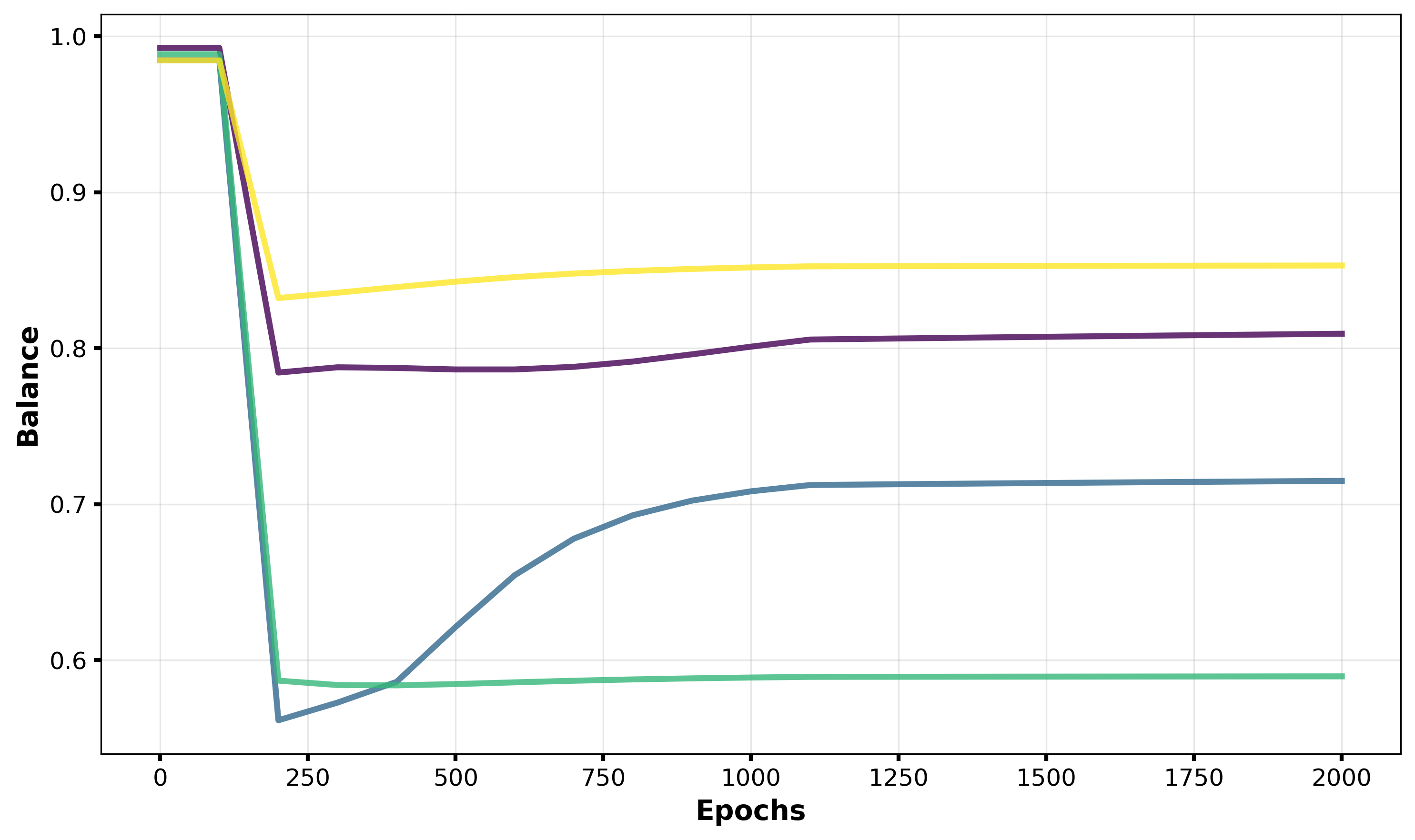
(a)

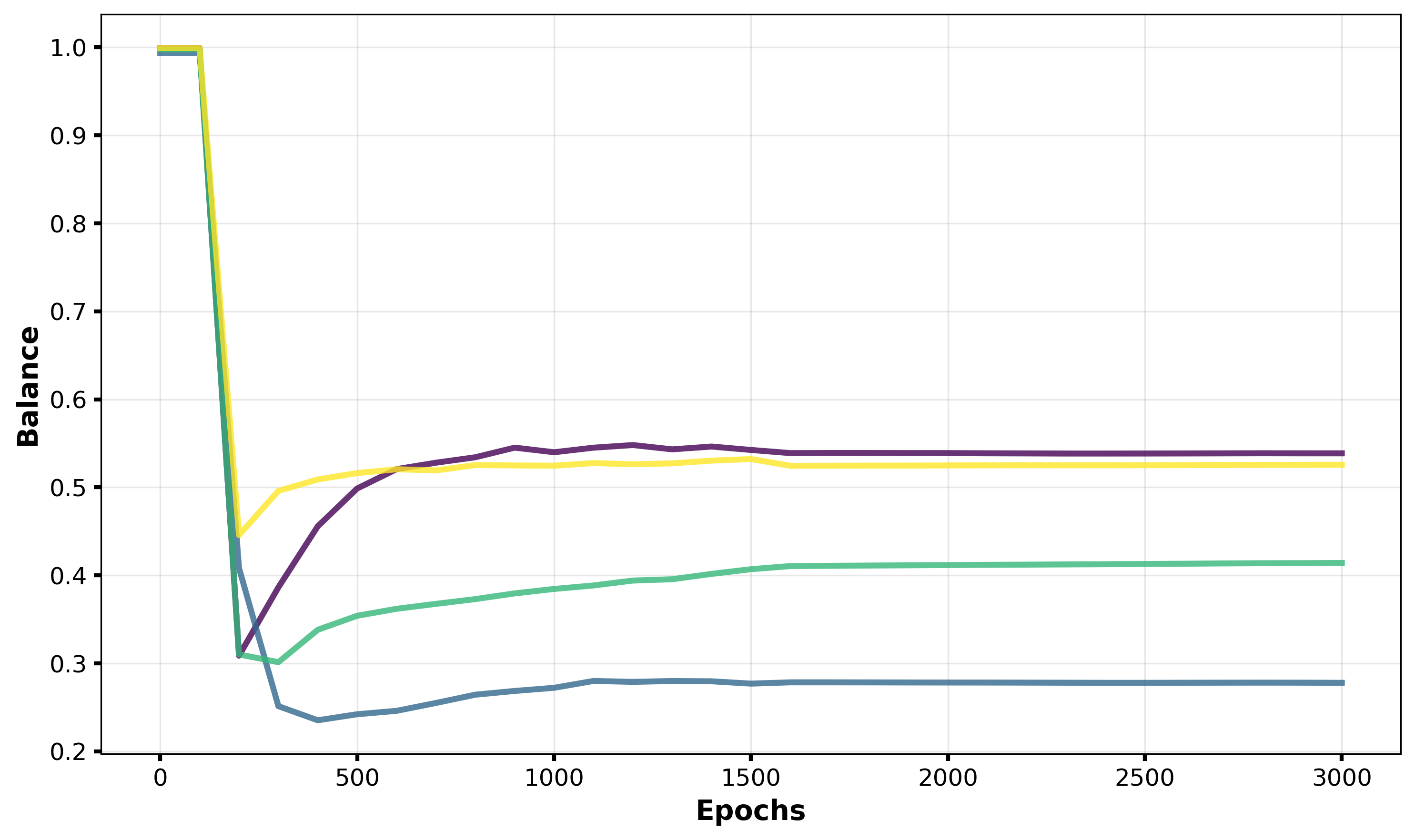
(b)

Figure 2: Normalized balancedness (see (25)) as a function of the number of training epochs, with each color representing an independent experiment.

References

• Andriopoulos et al., (2024) Andriopoulos, G., Dong, Z., Guo, L., Zhao, Z., and Ross, K. W. (2024). The prevalence of neural collapse in neural multivariate regression. In The Thirty-eighth Annual Conference on Neural Information Processing Systems.
• Araújo et al., (2019) Araújo, D., Oliveira, R. I., and Yukimura, D. (2019). A mean-field limit for certain deep neural networks. arXiv preprint arXiv:1906.00193.
• Beaglehole et al., (2024) Beaglehole, D., Súkeník, P., Mondelli, M., and Belkin, M. (2024). Average gradient outer product as a mechanism for deep neural collapse. In The Thirty-eighth Annual Conference on Neural Information Processing Systems.
• Chen et al., (2020) Chen, Z., Cao, Y., Gu, Q., and Zhang, T. (2020). A generalized neural tangent kernel analysis for two-layer neural networks. Advances in Neural Information Processing Systems, 33:13363–13373.
• (5) Fang, C., He, H., Long, Q., and Su, W. J. (2021a). Exploring deep neural networks via layer-peeled model: Minority collapse in imbalanced training. Proceedings of the National Academy of Sciences, 118(43):e2103091118.
• (6) Fang, C., Lee, J., Yang, P., and Zhang, T. (2021b). Modeling from features: a mean-field framework for over-parameterized deep neural networks. In Conference on learning theory, pages 1887–1936. PMLR.
• Han et al., (2022) Han, X., Papyan, V., and Donoho, D. L. (2022). Neural collapse under MSE loss: Proximity to and dynamics on the central path. In International Conference on Learning Representations.
• (8) Hong, W. and Ling, S. (2024a). Beyond unconstrained features: Neural collapse for shallow neural networks with general data. arXiv preprint arXiv:2409.01832.
• (9) Hong, W. and Ling, S. (2024b). Neural collapse for unconstrained feature model under cross-entropy loss with imbalanced data. Journal of Machine Learning Research, 25(192):1–48.
• Hu et al., (2021) Hu, K., Ren, Z., Šiška, D., and Szpruch, Ł. (2021). Mean-field langevin dynamics and energy landscape of neural networks. In Annales de l’Institut Henri Poincare (B) Probabilites et statistiques, volume 57, pages 2043–2065. Institut Henri Poincaré.
• Hui et al., (2022) Hui, L., Belkin, M., and Nakkiran, P. (2022). Limitations of neural collapse for understanding generalization in deep learning. arXiv preprint arXiv:2202.08384.
• Jacot et al., (2024) Jacot, A., Súkeník, P., Wang, Z., and Mondelli, M. (2024). Wide neural networks trained with weight decay provably exhibit neural collapse. arXiv preprint arXiv:2410.04887.
• Javanmard et al., (2020) Javanmard, A., Mondelli, M., and Montanari, A. (2020). Analysis of a two-layer neural network via displacement convexity. The Annals of Statistics, 48(6):3619–3642.
• Kim and Suzuki, (2024) Kim, J. and Suzuki, T. (2024). Transformers learn nonlinear features in context: Nonconvex mean-field dynamics on the attention landscape. In Forty-first International Conference on Machine Learning.
• Kothapalli, (2023) Kothapalli, V. (2023). Neural collapse: A review on modelling principles and generalization. Transactions on Machine Learning Research.
• Kothapalli and Tirer, (2024) Kothapalli, V. and Tirer, T. (2024). Kernel vs. kernel: Exploring how the data structure affects neural collapse. arXiv preprint arXiv:2406.02105.
• Lu et al., (2020) Lu, Y., Ma, C., Lu, Y., Lu, J., and Ying, L. (2020). A mean field analysis of deep resnet and beyond: Towards provably optimization via overparameterization from depth. In International Conference on Machine Learning, pages 6426–6436.
• Ma et al., (2022) Ma, C., Wu, L., et al. (2022). The barron space and the flow-induced function spaces for neural network models. Constructive Approximation, 55(1):369–406.
• Mei et al., (2019) Mei, S., Misiakiewicz, T., and Montanari, A. (2019). Mean-field theory of two-layers neural networks: dimension-free bounds and kernel limit. In Conference on learning theory, pages 2388–2464. PMLR.
• Mei et al., (2018) Mei, S., Montanari, A., and Nguyen, P.-M. (2018). A mean field view of the landscape of two-layer neural networks. Proceedings of the National Academy of Sciences, 115(33):E7665–E7671.
• Mixon et al., (2022) Mixon, D. G., Parshall, H., and Pi, J. (2022). Neural collapse with unconstrained features. Sampling Theory, Signal Processing, and Data Analysis, 20(2):11.
• Nguyen and Pham, (2023) Nguyen, P.-M. and Pham, H. T. (2023). A rigorous framework for the mean field limit of multilayer neural networks. Mathematical Statistics and Learning, 6(3):201–357.
• Nguyen and Mondelli, (2020) Nguyen, Q. N. and Mondelli, M. (2020). Global convergence of deep networks with one wide layer followed by pyramidal topology. Advances in Neural Information Processing Systems, 33:11961–11972.
• Pan and Cao, (2023) Pan, L. and Cao, X. (2023). Towards understanding neural collapse: The effects of batch normalization and weight decay. arXiv preprint arXiv:2309.04644.
• Papyan et al., (2020) Papyan, V., Han, X., and Donoho, D. L. (2020). Prevalence of neural collapse during the terminal phase of deep learning training. Proceedings of the National Academy of Sciences, 117(40):24652–24663.
• Pham and Nguyen, (2021) Pham, H. T. and Nguyen, P.-M. (2021). Global convergence of three-layer neural networks in the mean field regime. In International Conference on Learning Representations.
• Seleznova et al., (2024) Seleznova, M., Weitzner, D., Giryes, R., Kutyniok, G., and Chou, H.-H. (2024). Neural (tangent kernel) collapse. Advances in Neural Information Processing Systems, 36.
• Shevchenko et al., (2022) Shevchenko, A., Kungurtsev, V., and Mondelli, M. (2022). Mean-field analysis of piecewise linear solutions for wide relu networks. Journal of Machine Learning Research, 23(130):1–55.
• Shevchenko and Mondelli, (2020) Shevchenko, A. and Mondelli, M. (2020). Landscape connectivity and dropout stability of sgd solutions for over-parameterized neural networks. In International Conference on Machine Learning, pages 8773–8784. PMLR.
• Súkeník et al., (2024) Súkeník, P., Lampert, C. H., and Mondelli, M. (2024). Neural collapse vs. low-rank bias: Is deep neural collapse really optimal? In The Thirty-eighth Annual Conference on Neural Information Processing Systems.
• Súkeník et al., (2023) Súkeník, P., Mondelli, M., and Lampert, C. H. (2023). Deep neural collapse is provably optimal for the deep unconstrained features model. Advances in Neural Information Processing Systems, 36.
• (32) Suzuki, T., Wu, D., and Nitanda, A. (2024a). Mean-field langevin dynamics: Time-space discretization, stochastic gradient, and variance reduction. Advances in Neural Information Processing Systems, 36.
• (33) Suzuki, T., Wu, D., Oko, K., and Nitanda, A. (2024b). Feature learning via mean-field langevin dynamics: classifying sparse parities and beyond. Advances in Neural Information Processing Systems, 36.
• Takakura and Suzuki, (2024) Takakura, S. and Suzuki, T. (2024). Mean-field analysis on two-layer neural networks from a kernel perspective. In Forty-first International Conference on Machine Learning.
• Thrampoulidis et al., (2022) Thrampoulidis, C., Kini, G. R., Vakilian, V., and Behnia, T. (2022). Imbalance trouble: Revisiting neural-collapse geometry. In Advances in Neural Information Processing Systems.
• Tirer and Bruna, (2022) Tirer, T. and Bruna, J. (2022). Extended unconstrained features model for exploring deep neural collapse. In International Conference on Machine Learning, pages 21478–21505. PMLR.
• Wainwright, (2019) Wainwright, M. J. (2019). High-Dimensional Statistics: A Non-Asymptotic Viewpoint. Cambridge Series in Statistical and Probabilistic Mathematics. Cambridge University Press.
• Zhou et al., (2022) Zhou, J., Li, X., Ding, T., You, C., Qu, Q., and Zhu, Z. (2022). On the optimization landscape of neural collapse under mse loss: Global optimality with unconstrained features. In International Conference on Machine Learning, pages 27179–27202. PMLR.