Understanding Oversmoothing in GNNs as Consensus in Opinion Dynamics
Abstract
In contrast to classes of neural networks where the learned representations become increasingly expressive with network depth, the learned representations in graph neural networks (GNNs), tend to become increasingly similar. This phenomena, known as oversmoothing, is characterized by learned representations that cannot be reliably differentiated leading to reduced predictive performance. In this paper, we propose an analogy between oversmoothing in GNNs and consensus or agreement in opinion dynamics. Through this analogy, we show that the message passing structure of recent continuous-depth GNNs is equivalent to a special case of opinion dynamics (i.e., linear consensus models) which has been theoretically proven to converge to consensus (i.e., oversmoothing) for all inputs. Using the understanding developed through this analogy, we design a new continuous-depth GNN model based on nonlinear opinion dynamics and prove that our model, which we call behavior-inspired message passing neural network (BIMP) circumvents oversmoothing for general inputs. Through extensive experiments, we show that BIMP is robust to oversmoothing and adversarial attack, and consistently outperforms competitive baselines on numerous benchmarks.
1 Introduction
Graphs can be used to describe observations in diverse contexts, such as molecular dynamics (Fang et al., 2022), biological behavior, and computer networking. Graph neural networks (GNNs) leverage this structure to learn the features of the nodes and edges within these systems. Numerous GNN architectures have been proposed, including graph convolutional networks, (GCN) (Kipf & Welling, 2016), graph attention networks (GAT) (Veličković et al., 2017) GraphSAGE (Hamilton et al., 2017), and message passing neural networks (Gilmer et al., 2017). These methods respect the permutation equivariance of the underlying graph through constraints on the node and edge aggregation functions. However, it is exactly the structure of these aggregation functions that leads to oversmoothing, a phenomenon where network features become increasingly indistinguishable with increasing network depth (Oono & Suzuki, 2019; Nt & Maehara, 2019).
Recent works address oversmoothing in three different ways (Rusch et al., 2023): using residual connections (Li et al., 2019; Chen et al., 2020b; Xu et al., 2018; Liu et al., 2020); regularizing node features (Li et al., 2019; Chen et al., 2020b; Xu et al., 2018; Liu et al., 2020); and using physical inductive biases as message-passing functions.
This last approach is commonly used in continuous-depth GNN models where node features are propagated forward in time using a continuous-time differential equation rather than the discrete layerwise transformations of conventional message-passing architectures. Dynamical equations such as the diffusion equation (Chamberlain et al., 2021b; Thorpe et al., 2022), wave equation (Eliasof et al., 2021), coupled oscillator equations (Rusch et al., 2022; Nguyen et al., 2024), Allen-Cahn equation for particle systems (Wang et al., 2022), and geometrical equations like Beltrami flows (Chamberlain et al., 2021a) and Racci flows (Topping et al., 2021) have been successfully applied in this context.
Instead of using physical inductive biases to model the evolution of node features, we propose the use of opinion dynamics, a multi-agent systems model that captures the evolution of agent opinions (or node features in our case) over time (Zha et al., 2020; Dong et al., 2021; Montes de Oca et al., 2010). While the evolution of agent opinions converge for all initial conditions under a linear opinion dynamics model, the opinions of agents can have diverse outcomes under the nonlinear opinion dynamics (NOD) model (Bizyaeva et al., 2022; Leonard et al., 2024). This flexibility is due to the nonlinearity in NOD which introduces a bifurcation, allowing opinions to move toward consensus or dissensus (i.e., not consensus) depending on the initial conditions and network connectivity.
In this paper, we propose an analogy between oversmoothing in GNNs and opinion consensus in opinion dynamics models leading to the following contributions:
-
•
We prove that the dynamics of recent continuous-depth GNN models are equivalent to linear opinion dynamics and will consequently exhibit oversmoothing for all initial conditions,
-
•
We design a novel continuous-depth GNN model using a nonlinear opinion dynamics inductive bias, and prove that our behavior-inspired message passing (BIMP) model has greater expressive capacity than other continuous-depth GNN models,
-
•
We perform extensive empirical analysis and show that our BIMP model consistently outperforms competitive baseline models.
2 Related Work
Oversmoothing in graph neural networks.
Oversmoothing problem is widely noticed and discussed in (Li et al., 2018; Oono & Suzuki, 2019; Nt & Maehara, 2019). As the learned embeddings get similar, oversmoothing can be interpreted as an expressivity decay which is often analyzed using the Weisfeiler-Lehman test (Huang & Villar, 2021). Recent works provide precise definitions of oversmoothing through various perspectives, including the feature distance (Chen et al., 2020a), Dirichlet energy (Cai & Wang, 2020; Zhou et al., 2021; Rusch et al., 2022, 2023) and information gain (Zhou et al., 2020). Given these definitions, however, finding an efficient method to mitigate oversmoothing remains challenging and attracts significant attention in GNNs research.
Continuous-depth graph neural networks.
Continuous-depth networks such as NODE (Chen et al., 2018) define the network depth implicitly via the simulation of the given differential equations. Further work presented a framework (Poli et al., 2019) where inputs propagate through a continuum of GNN layers for a continuous-depth GNN. Extensions to this concept embeds many physical systems as the differential equation in continuous-depth GNNs. Rusch et al. (2022) leverages the stability characteristics in coupled oscillators to tackle the oversmoothing problem; Wang et al. (2022) incorporates the Allen-Cahn reaction-diffusion to achieve stricter lower-bounds on the Dirichlet energy for GNNs; Nguyen et al. (2024) models the underlying dynamics as oscillators in a Kuramoto system to reformulate oversmoothing as a problem of synchronization.
Opinion dynamics.
Since opinions can be interpreted as latent preferences, modeling opinion dynamics provides insights into understanding and predicting agents’ behavior. Specifically, consensus dynamics (Bullo, 2018) is commonly used to model the coordination of multi-agent systems. Leonard et al. (2010) describe a linear consensus dynamics for coordinated surveying with underwater gliders. Justh & Krishnaprasad (2005) use the consensus dynamics framework to formulate rectilinear and circular control laws for a multi-vehicles system. In (Leonard et al., 2007), the authors use consensus dynamics to improve data collection coverage in a mobile sensor network. Ballerini et al. (2008) use consensus dynamics to understand the robustness of starling flocking behavior. However, there are several draw backs to using a linear model for opinion formulation; specifically, the naive implementation results in dynamics that only converge to consensus (Altafini, 2012; Dandekar et al., 2013).
Nonlinear opinion dynamics.
The noted short comings of consensus dynamics models are resolved in the nonlinear opinion dynamics (Leonard et al., 2024). The nonlinearity of the model results in bifurcations (Golubitsky et al., 2012; Guckenheimer & Holmes, 2013; Strogatz, 2018) and opinions can evolve to dissensus rapidly even under weak input signals (Bizyaeva et al., 2022). Nonlinear opinion dynamics have been shown to able to model a variety of systems such as political polarization (Leonard et al., 2021); group decision making (Dong et al., 2021); multi-agent control (Montes de Oca et al., 2010; Leonard et al., 2010; Cathcart et al., 2023); and relational inference (Yang et al., 2024). Our proposed network seeks to integrate nonlinear opinion dynamics as the behavior-inspired inductive bias in a continuous-depth GNN.
3 Preliminaries
In this section we describe our notation and review nonlinear opinion dynamics (Leonard et al., 2024).
3.1 Notation
Throughout this text we use lower-case letters for scalar valued variables, boldface lower-case letters for vectors, and boldface upper-case letters for matrices. We define graphs as the set with nodes and . For multi-agent system evolving under opinion dynamics models we use to denote the number of agents and to denote the number of options.
3.2 Nonlinear opinion dynamics
Nonlinear opinion dynamics captures the evolution of agent opinions in a multi-agent system. Opinions for each option can be positive, neutral, or negative, where the magnitude correlates to the opinion strength. Changes to these opinions are affected by extrinsic and intrinsic parameters. Specifically, agent ’s opinion about option can be described by the following nonlinear differential equation proposed in (Bizyaeva et al., 2022; Leonard et al., 2024),
| (1) |
The parameters , , and are intrinsic to each agent. The damping term describes the resilience of agent to forming an opinion on option ; the attention represents the attentiveness of agent to the opinions of other agents; and the self-reinforcement defines the resistance of agent to changing the opinion for option .
The parameters , , and , and saturating function are extrinsic to the agents. The environmental represents the impact of the environment on the agent’s opinion for option . The saturating function is selected so that , , and . We use a hyperbolic tangent for the saturation function in our method.
The communication network graph describes how agents are able to exchange their opinions over time. The communication adjacency matrix defines the communication strength between agent and agent . Similarly, the belief system graph describes the correlation between options. The belief adjacency matrix defines the strength of correlation between option and .
4 Understanding Oversmoothing with Opinion Dynamics
In this section, we propose an analogy between GNNs and opinion dynamics models, and use our analogy to: (1) prove that recent continuous-depth GNN dynamics will exhibit oversmoothing for all inputs; and (2) design a novel continuous-depth GNN, behavior-inspired message passing (BIMP) GNN, using a nonlinear opinion dynamics inductive bias to circumvent oversmoothing and improve expressivity.
4.1 Oversmoothing is Opinion Consensus
Oversmoothing.
In the GNN literature, oversmoothing is loosely defined as the exponential convergence of node features with increasing network depth. A precise definition of oversmoothing is given in (Rusch et al., 2023).
The degree of oversmoothing in a network can be measured by the Dirichlet energy (Cai & Wang, 2020; Rusch et al., 2023) defined,
| (2) |
where denotes the feature associated with node at layer . Oversmoothing is said to occur when the Dirichlet energy of layer tends to zero as tends to infinity, which is equivalent to the condition,
| (3) |
Linear opinion dynamics.
Opinion dynamics models describe the evolution of agent opinions in a multi-agent system. The linear opinion dynamics model introduced in (DeGroot, 1974) describes the discrete-time evolution of agent opinions by
| (4) |
where denotes the influence of agent on agent , and the total influence of any agent sums to one. The continuous-time analogue can be expressed,
| (5) |
A limitation of linear opinion dynamics models, is that the opinions of agents tend toward consensus (i.e., agreement) for all initial conditions. Moreover, the consensus value is independent of the graph structure and linearly dependent on the initial conditions (Leonard et al., 2024).
Opinion consensus.
An opinion dynamics model is said to reach consensus if and only if the opinions of all agents tend toward the same value as time tends to infinity, that is,
| (6) |
GNN-OD Analogy
We construct an analogy between GNNs and opinion dynamics models to guide our analysis of existing continuous-time GNNs, and the development of our new continuous-time GNN, BIMP. Our analogy likens nodes at layer of a GNN with agents at time in a multi-agent system, node features with agent opinions, and oversmoothing with opinion consensus. The analogy is summarized in Table 1.
| Graph neural networks | Opinion dynamics |
|---|---|
| Node | Agent |
| Edge | Communication link |
| Node feature dimension | Number of agent options |
| Value of node feature | Opinion of agent option |
| Oversmoothing | Opinion consensus |
4.2 Oversmoothing in GRAND
Using our graph neural network, opinion dynamics analogy we show that the recently introduced continuous-depth GNN model graph neural diffusion (GRAND) (Chamberlain et al., 2021b) and its variants exhibit oversmoothing in the limit.
Linear GRAND (GRAND-).
In GRAND, information is exchanged between nodes according to the diffusion process,
| (7) |
where , for some similarity measure evaluated over all connected nodes (i.e., ).
Linear GRAND (GRAND-), is a special case of GRAND with time-independent . In this case, the similarity measure is defined using multi-head attention (Vaswani, 2017),
| (8) |
where and are learned matrices with dimension . In this case, the dynamics can be expressed,
| (9) |
where . Since , is right stochastic, the dynamical equation for GRAND- is equivalent to the dynamical equation for linear opinion dynamics (see Equation 5) and in the limit, GRAND- will exhibit oversmoothing.
Proposition 4.1.
In the limit GRAND- will exhibit oversmoothing.
Proof.
By distributing and rearranging terms in Equation(9), the dynamics of GRAND- can be expressed,
| (10) |
Since is constrained to be right stochastic the dynamics are equivalent to those of the linear opinion dynamics model in Equation (4). Consequently, all nodes will converge to the same value. This is the consensus/oversmoothing condition described in Equations (6) and (2). ∎
Adding a damping term does not resolve oversmoothing.
GraphCON (Rusch et al., 2022) introduces a framework to mitigate oversmoothing in continuous-depth GNNs by stabilizing the time evolution of the Dirichlet energy. This is achieved by amending an arbitrary GNN with damping terms and converting it to a continuous-depth model. The dynamical update for a GraphCON amended GNN is given by,
| (11) |
where is the activation function, and and are damping terms that force the dynamics converge to a desired equilibrium.
In GraphCON-Tran (Rusch et al., 2022), the authors amend GRAND- with the GraphCON framework and achieve improved performance at increased network depths. The dynamics of the GraphCON-Tran model is given by
| (12) |
Here is the identity mapping, , and . The corresponding steady solution is
| (13) |
which is equivalent to GRAND- (see Equation (9)), so GraphCON-Tran will exhibit oversmoothing.
Adding a source term is not the perfect answer.
In GRAND++ (Thorpe et al., 2022), the authors amend GRAND with a source term to alleviate oversmoothing. The dynamical update for GRAND++ is given by,
| (14) |
where is the index set of nodes whose features are used to compute the source term, and is a function of .
GRAND++- is a special case of GRAND++ with time-independent ,
| (15) |
While the performance of GRAND++- exceeds that of GRAND-, the performance boost comes at the expense of the system equilibrium. Moreover, for large timescales, the difference in node features is relatively small resulting in reduced discriminability, and poorer network performance.
Proposition 4.2.
As the dynamics of GRAND++- are approximately linear in .
5 BIMP: Behavior-Inspired Message Passing Neural Network
In this section, we introduce our BIMP model. We show that by incorporating nonlinear opinion dynamics as an inductive bias we circumvent oversmoothing and retain expressivity.
5.1 Formulation
In our proposed BIMP model, information is exchanged between nodes according the nonlinear opinion dynamics model,
| (16) |
where we set , and . The flexibility of nonlinear opinion dynamics allows BIMP to model more diverse node feature representations than approaches whose dynamics are equivalent to linear opinion dynamics.
5.2 GRAND- is a first-order approximation of BIMP
Proposition 5.1.
For a BIMP model with attention parameter , bias parameter , and uncorrelated options , the first-order approximation is equivalent to GRAND-.
Proof.
The BIMP model described in the proposition has dynamics of the form
| (17) |
When , , so is an equilibrium of the system. The first-order approximation of our model dynamics about this equilibrium is given by
| (18) |
When , this equation reduces to,
| (19) |
which is of the same form as GRAND- (see Equation (7)). Since GRAND- has the same form as the first-order approximation of our BIMP model, we say our BIMP model has greater expressive capacity. ∎
5.3 Designing an expressive BIMP model
The effective adjacency matrix.
To ensure our model has the expected behavior, the effective adjacency matrix must be constrained to have a simple leading eigenvalue (Leonard et al., 2024). In (Leonard et al., 2024) the authors consider a nonlinear opinion dynamics model of the form
| (20) |
where the communication matrix has a simple leading eigenvalue. We consider the general form of nonlinear opinion dynamics given in Equation (16) and show that it can be reduced to Equation (20) with the following definition for the effective adjacency matrix.
Definition 5.2.
Given the communication matrix and belief matrix , the effective adjacency matrix is defined
| (21) |
where denotes the Kronecker product.
Given this definition, we have the following proposition.
Proposition 5.3.
Proof.
We first rewrite Equation (16) in the following form:
| (22) |
From here, we can write the matrix product with , and , as , where denotes the vectorization operator (Magnus & Neudecker, 2019). This yields the following form
| (23) |
where , and follows from Definition 5.2. Vectorizing both sides of yields
| (24) |
where , and . We obtain the general nonlinear opinion dynamics in the form (20). ∎
Leveraging Proposition 5.3 we can say that if the effective adjacency matrix has a simple leading eigenvalue the system will exhibit the expected behavior.
The condition on the effective adjacency matrix is satisfied by a right-stochastic matrix (the leading eigenvalue of a right-stochastic matrix is ), however, the size of the effective adjacency matrix (i.e., ) would impose a computational challenge. To circumvent this, we instead learn the communication matrix and belief matrix separately. Specifically, the entries of the communication matrix are defined using multi-head attention,
| (25) |
where and are the key and query weight matrices, and is the attention dimension. is the opinion of agent . The entries of the belief matrix are defined similarly,
| (26) |
where and are the key and query weight matrices, and is the attention dimension.
The attention parameter.
For our model to utilize its expressive capacity, it must not degenerate to a linear model. The degenerate form occurs both when is very small, since the nonlinear term evaluates to zero, and when is very large, since the nonlinear term evaluates to one. To avoid this, we set the attention to the critical point of the attention-opinion bifurcation diagram.
Proposition 5.4.
The critical point of the attention-opinion bifurcation diagram is equal to .
Proof.
The critical point of the attention-opinion bifurcation diagram occurs when the bias parameter is equal to zero and agent opinions are at equilibrium.
Following (Leonard et al., 2024), we use a linear analysis to determine the critical point of the attention-opinion bifurcation diagram. The linearization of the nonlinear opinion dynamics model (Equation (24)) is given by , where is the Jacobian evaluated at the equilibrium , and . At the equilibrium , the Jacobian is given by
| (27) |
The eigenvalue of the Jacobian determines the equilibrium stability. Denoting the eigenvalue of , , the eigenvalue of the Jacobian can be expressed,
| (28) |
The critical point of the attention-opinion bifurcation diagram occurs when the dominant eigenvalue of the Jacobian is zero. Solving for the critical value of the attention yields . ∎
To obtain a value for the attention, we must know the value for , , and . While we treat and as hyperparameters of our model, is determined by the structure of our effective adjacency matrix.
Proposition 5.5.
The dominant eigenvalue of is equal to four.
Proof.
Since both the communication matrix and the belief matrix are right stochastic, their dominant eigenvalues are equal to one (i.e., ). Since , its dominant eigenvalue is equal to . ∎
BIMP equilibrium behavior.
With our choice of effective adjacency matrix and attention parameter , BIMP converges to equilibrium when the input parameter is constant.
Proposition 5.6.
A BIMP model with time-independent bias parameter converges to an equilibrium.
We prove Proposition 5.6 in Appendix A.2 by showing that the nonlinear opinion dynamics are monotone and bounded. Consequently, there are no dynamical behaviors other than convergence to an equilibrium. Since all trajectories tend toward the equilibrium solution, analyzing the equilibrium behavior is sufficient to understand the dynamics of BIMP.
The bias parameter
We can show that if the input parameter is chosen to be nonzero, BIMP can achieve dissensus (i.e., will not exhibit oversmoothing). We first explore the behavior of BIMP when the input parameter is equal to zero.
Proposition 5.7.
When the bias parameter is equal to zero, the dynamics of BIMP can be approximated by the dynamics of the reduced one-dimensional dynamical equation.
| (29) |
where , and is the left dominant eigenvector of .
Following (Leonard et al., 2024), we use the Lyapunov–Schmidt reduction (Golubitsky & Schaeffer, 1985) to determine the reduced model. We decompose our BIMP’s dynamics into a critical subspace and a regular subspace. The critical subspace corresponds to the zero eigenvalue of linearized system, which governs the long-term behavior (i.e., equilibrium). In contrast, the regular subspace corresponds to the negative eigenvalues of the linearized system, which decays quickly and have a limited contribution to the long-term dynamics. It is therefore sufficient to focus on the critical subspace to understand the dynamics of the equilibrium as the regular subspace decays quickly. We derive Equation (47) in Appendix A.3.
Proposition 5.8.
BIMP exhibits oversmoothing when the bias parameter is equal to zero.
Proof.
For in the neighborhood of the equilibrium , the right-hand side of Equation (47) is isomorphic to , and at the critical point Equation (47) has unique equilibrium . This corresponds to an equilibrium solution of in the original system (Equation (24)) which means that and all agents form neutral opinions for all options. Since the opinions of all agents have converged, the system has reached consensus (i.e., exhibits oversmoothing). ∎
Proposition 5.9.
BIMP will not exhibit oversmoothing when the bias parameter is time-independent with unique entries.
A distinct and time-independent serves as a constant forcing term that applies a continuous influence on each opinion , biasing the evolution of toward . Consequently, the system equilibrium is shifted and opinions reach dissensus. We prove Proposition 5.9 in Appendix A.4.
To ensure satisfies the conditions of Proposition 5.9, we we set to the initial opinion state, i.e., . A similar strategy is used GRAND++ (Thorpe et al., 2022) and KuramotoGNN (Nguyen et al., 2024).
| Dataset | BIMP (ours) | GRAND- | GRAND++- | KuramotoGNN | GraphCON | GAT | GCN | GraphSAGE |
|---|---|---|---|---|---|---|---|---|
| Cora | 83.191.13 | 82.201.45 | 82.831.31 | 81.161.61 | 82.801.34 | 79.761.50 | 80.762.04 | 79.371.70 |
| Citeseer | 71.091.40 | 69.891.48 | 70.261.46 | 70.401.02 | 69.601.16 | 67.701.63 | 67.541.98 | 67.311.63 |
| Pubmed | 80.162.03 | 78.191.88 | 78.891.96 | 78.691.91 | 78.851.53 | 76.882.08 | 77.041.78 | 75.522.19 |
| CoauthorCS | 92.480.26 | 90.230.91 | 90.100.78 | 91.050.56 | 90.300.74 | 89.510.54 | 90.980.42 | 90.620.42 |
| Computers | 84.730.61 | 82.930.56 | 82.790.54 | 80.061.60 | 82.760.58 | 81.731.89 | 82.021.87 | 76.427.60 |
| Photo | 92.900.44 | 91.930.39 | 91.510.41 | 92.770.42 | 91.780.50 | 89.121.60 | 90.371.38 | 88.712.68 |
5.4 BIMP training behavior
We can show that even for very deep networks, BIMP gradients will not explode or exponentially vanish during training.
Proposition 5.10.
BIMP gradients are upper-bounded when the step-size and damping term .
Proposition 5.11.
BIMP gradients will not vanish exponentially when the step-size and the damping term .
6 Experiments
In this section, we highlight our model’s improved robustness to oversmoothing compared to competitive baselines, strong performance on graph classification tasks, and resilience to adversarial attack.
6.1 Robustness to oversmoothing
We measure oversmoothing in GCN (Kipf & Welling, 2016), GAT (Veličković et al., 2017), GRAND- (Chamberlain et al., 2021b), GRAND++- (Thorpe et al., 2022), GraphCON-Tran (Rusch et al., 2022) and our BIMP model across network depths using the Dirichlet energy (see Equation (2)), and plot the results in Figure 2. The Dirichlet energy of our BIMP model is stable out to 1000 layers while the energy of other models decreases (i.e., approaches oversmoothing). Additional experimental details are provided in Appendix C.2.1.
To understand the impact of oversmoothing on classification accuracy, we compare the performance of our BIMP model, GRAND- , GRAND++- and GraphCON-Tran on the Cora (McCallum et al., 2000), Citeseer (Sen et al., 2008) and Pubmed (Namata et al., 2012) datasets. Each model is trained over a range of network depths and fixed hyperparameters; results are reported in Figure 1. Our BIMP model has comparable performance with baseline models when networks depths are small, but increasingly better performance compared to baseline models as network depths increase. Additional experimental details are provided in Appendix C.2.2.
6.2 Improved classification accuracy
We demonstrate improved classification performance compared to GRAND-, GRAND-, KuramotoGNN, GraphCON, GAT, GCN, and GraphSAGE on the Cora, Citeseer, Pubmed, Computers (Shchur et al., 2018), CoauthorCS (Shchur et al., 2018), and Photo (Shchur et al., 2018) datasets. Classification accuracies are reported in Table 2, where BIMP consistently outperforms baseline models. We also observe the improved performance on heterophilic datasets reported in Table 7 in Appendix D.2.
6.3 Resilience to adversarial attack
We demonstrate improved resilience to adversarial attack compared to GRAND- under random and PGD (Mkadry et al., 2017) attack methods on the Cora, Citeseer and Pubmed datasets. We use an untargeted graph modification attack, perturbingnode features at inference. In the random attack, we sample the perturbation from , and in the PGD attack, we choose . Classification accuracies are reported in Table 3, and show that our BIMP model significantly outperforms the baseline model.
6.4 Computational complexity
We compare the space complexity of our BIMP model with that of GRAND-. The complexity our model is , where is the number of edges, is the number of nodes, and is the feature dimension. The space complexity of our model is comparable to GRAND-, which has complexity ).
We also compute the time complexity of our model. We compare the average run time of our model against baseline models in Table 6 of Appendix C.4. Despite incorporating nonlinearity and belief matrix , BIMP has comparable run time performance to linear baselines models. Additional experimental details are provided in Appendix C.4.
| Dataset | Attack method | BIMP (ours) | GRAND- |
|---|---|---|---|
| Cora | Clean | 82.42.1 | 82.11.4 |
| Random | 70.81.6 | 61.62.3 | |
| PGD | 56.45.4 | 38.44.9 | |
| Citeseer | Clean | 70.41.6 | 70.01.7 |
| Random | 57.81.2 | 42.52.2 | |
| PGD | 57.43.1 | 39.63.7 | |
| Pubmed | Clean | 79.71.9 | 78.32.1 |
| Random | 61.26.7 | 40.82.5 | |
| PGD | 40.17.8 | 37.65.6 |
7 Conclusion
In this paper, we propose an analogy between GNNs and opinion dynamics models highlighting the equivalence between the oversmoothing condition in GNNs and consensus condition in opinion dynamics. Through our analogy, we show that recent continuous-depth GNNs are equivalent to linear opinion dynamics models, which are proven to converges to consensus. To address this issue, we introduce a novel class of continuous-depth GNNs called Behavior-inspired message passing (BIMP) neural networks which leverage the nonlinear opinion dynamics inductive bias. The nonlinear saturation function and distinct bias in BIMP results in greater expressivity and guaranteed dissensus. Experiments against competitive baselines illustrate our model’s robustness to network depth, improved expressivity, and resiliance to adversarial attack.
Limitation and Future work
With large step sizes, the damping term leads to training instability, limiting training acceleration with large time scales. Future work will develop deeper insights into the effect of the nonlinearity in BIMP on its resilience to adversarial attacks.
Impact statement
We present a novel continuous-depth graph neural networks to tackle the oversmoothing issue and enable us to build a deep model with enhanced expressive capacity. The improved expressivity can lead to some breakthroughs in various domains such as drug discovery and protein prediction, where we don’t anticipate the negative societal impacts.
References
- Altafini (2012) Altafini, C. Consensus problems on networks with antagonistic interactions. IEEE transactions on automatic control, 58(4):935–946, 2012.
- Ballerini et al. (2008) Ballerini, M., Cabibbo, N., Candelier, R., Cavagna, A., Cisbani, E., Giardina, I., Lecomte, V., Orlandi, A., Parisi, G., Procaccini, A., et al. Interaction ruling animal collective behavior depends on topological rather than metric distance: Evidence from a field study. Proceedings of the national academy of sciences, 105(4):1232–1237, 2008.
- Bizyaeva et al. (2022) Bizyaeva, A., Franci, A., and Leonard, N. E. Nonlinear opinion dynamics with tunable sensitivity. IEEE Transactions on Automatic Control, 68(3):1415–1430, 2022.
- Bullo (2018) Bullo, F. Lectures on network systems, volume 1. CreateSpace, 2018.
- Cai & Wang (2020) Cai, C. and Wang, Y. A note on over-smoothing for graph neural networks. arXiv preprint arXiv:2006.13318, 2020.
- Cathcart et al. (2023) Cathcart, C., Santos, M., Park, S., and Leonard, N. E. Proactive opinion-driven robot navigation around human movers. In 2023 IEEE/RSJ International Conference on Intelligent Robots and Systems (IROS), pp. 4052–4058, 2023. doi: 10.1109/IROS55552.2023.10341745.
- Chamberlain et al. (2021a) Chamberlain, B., Rowbottom, J., Eynard, D., Di Giovanni, F., Dong, X., and Bronstein, M. Beltrami flow and neural diffusion on graphs. Advances in Neural Information Processing Systems, 34:1594–1609, 2021a.
- Chamberlain et al. (2021b) Chamberlain, B., Rowbottom, J., Gorinova, M. I., Bronstein, M., Webb, S., and Rossi, E. Grand: Graph neural diffusion. In International conference on machine learning, pp. 1407–1418. PMLR, 2021b.
- Chen et al. (2020a) Chen, D., Lin, Y., Li, W., Li, P., Zhou, J., and Sun, X. Measuring and relieving the over-smoothing problem for graph neural networks from the topological view. In Proceedings of the AAAI conference on artificial intelligence, volume 34, pp. 3438–3445, 2020a.
- Chen et al. (2020b) Chen, M., Wei, Z., Huang, Z., Ding, B., and Li, Y. Simple and deep graph convolutional networks. In International conference on machine learning, pp. 1725–1735. PMLR, 2020b.
- Chen et al. (2018) Chen, R. T., Rubanova, Y., Bettencourt, J., and Duvenaud, D. K. Neural ordinary differential equations. Advances in neural information processing systems, 31, 2018.
- Craven et al. (1998) Craven, M., DiPasquo, D., Freitag, D., McCallum, A., Mitchell, T., Nigam, K., and Slattery, S. Learning to extract symbolic knowledge from the world wide web. AAAI/IAAI, 3(3.6):2, 1998.
- Dandekar et al. (2013) Dandekar, P., Goel, A., and Lee, D. T. Biased assimilation, homophily, and the dynamics of polarization. Proceedings of the National Academy of Sciences, 110(15):5791–5796, 2013.
- DeGroot (1974) DeGroot, M. H. Reaching a consensus. Journal of the American Statistical association, 69(345):118–121, 1974.
- Dong et al. (2021) Dong, Y., Zha, Q., Zhang, H., and Herrera, F. Consensus reaching and strategic manipulation in group decision making with trust relationships. IEEE Transactions on Systems, Man, and Cybernetics: Systems, 51(10):6304–6318, 2021. doi: 10.1109/TSMC.2019.2961752.
- Eliasof et al. (2021) Eliasof, M., Haber, E., and Treister, E. Pde-gcn: Novel architectures for graph neural networks motivated by partial differential equations. Advances in neural information processing systems, 34:3836–3849, 2021.
- Fang et al. (2022) Fang, X., Liu, L., Lei, J., He, D., Zhang, S., Zhou, J., Wang, F., Wu, H., and Wang, H. Geometry-enhanced molecular representation learning for property prediction. Nature Machine Intelligence, 4(2):127–134, 2022.
- Fey & Lenssen (2019) Fey, M. and Lenssen, J. E. Fast graph representation learning with pytorch geometric. arXiv preprint arXiv:1903.02428, 2019.
- Gilmer et al. (2017) Gilmer, J., Schoenholz, S. S., Riley, P. F., Vinyals, O., and Dahl, G. E. Neural message passing for quantum chemistry. In International conference on machine learning, pp. 1263–1272. PMLR, 2017.
- Golubitsky & Schaeffer (1985) Golubitsky, M. and Schaeffer, D. G. Singularities and Groups in Bifurcation Theory, Volume I, volume 51 of Applied Mathematical Sciences. Springer-Verlag, New York, 1985.
- Golubitsky et al. (2012) Golubitsky, M., Stewart, I., and Schaeffer, D. G. Singularities and Groups in Bifurcation Theory: Volume II, volume 69. Springer Science & Business Media, 2012.
- Guckenheimer & Holmes (2013) Guckenheimer, J. and Holmes, P. Nonlinear oscillations, dynamical systems, and bifurcations of vector fields, volume 42. Springer Science & Business Media, 2013.
- Hamilton et al. (2017) Hamilton, W., Ying, Z., and Leskovec, J. Inductive representation learning on large graphs. Advances in neural information processing systems, 30, 2017.
- Hirsch (1985) Hirsch, M. W. Systems of differential equations that are competitive or cooperative ii: Convergence almost everywhere. SIAM Journal on Mathematical Analysis, 16(3):423–439, 1985.
- Huang & Villar (2021) Huang, N. T. and Villar, S. A short tutorial on the weisfeiler-lehman test and its variants. In ICASSP 2021-2021 IEEE International Conference on Acoustics, Speech and Signal Processing (ICASSP), pp. 8533–8537. IEEE, 2021.
- Justh & Krishnaprasad (2005) Justh, E. W. and Krishnaprasad, P. Natural frames and interacting particles in three dimensions. In Proceedings of the 44th IEEE Conference on Decision and Control, pp. 2841–2846. IEEE, 2005.
- Kipf & Welling (2016) Kipf, T. N. and Welling, M. Semi-supervised classification with graph convolutional networks. arXiv preprint arXiv:1609.02907, 2016.
- Leonard et al. (2007) Leonard, N. E., Paley, D. A., Lekien, F., Sepulchre, R., Fratantoni, D. M., and Davis, R. E. Collective motion, sensor networks, and ocean sampling. Proceedings of the IEEE, 95(1):48–74, 2007.
- Leonard et al. (2010) Leonard, N. E., Paley, D. A., Davis, R. E., Fratantoni, D. M., Lekien, F., and Zhang, F. Coordinated control of an underwater glider fleet in an adaptive ocean sampling field experiment in monterey bay. Journal of Field Robotics, 27(6):718–740, 2010.
- Leonard et al. (2021) Leonard, N. E., Lipsitz, K., Bizyaeva, A., Franci, A., and Lelkes, Y. The nonlinear feedback dynamics of asymmetric political polarization. Proceedings of the National Academy of Sciences, 118(50):e2102149118, 2021.
- Leonard et al. (2024) Leonard, N. E., Bizyaeva, A., and Franci, A. Fast and flexible multiagent decision-making. Annual Review of Control, Robotics, and Autonomous Systems, 7, 2024.
- Li et al. (2019) Li, G., Muller, M., Thabet, A., and Ghanem, B. Deepgcns: Can gcns go as deep as cnns? In Proceedings of the IEEE/CVF international conference on computer vision, pp. 9267–9276, 2019.
- Li et al. (2018) Li, Q., Han, Z., and Wu, X.-M. Deeper insights into graph convolutional networks for semi-supervised learning. In Proceedings of the AAAI conference on artificial intelligence, volume 32, 2018.
- Liaw et al. (2018) Liaw, R., Liang, E., Nishihara, R., Moritz, P., Gonzalez, J. E., and Stoica, I. Tune: A research platform for distributed model selection and training. arXiv preprint arXiv:1807.05118, 2018.
- Liu et al. (2020) Liu, M., Gao, H., and Ji, S. Towards deeper graph neural networks. In Proceedings of the 26th ACM SIGKDD international conference on knowledge discovery & data mining, pp. 338–348, 2020.
- Magnus & Neudecker (2019) Magnus, J. R. and Neudecker, H. Matrix differential calculus with applications in statistics and econometrics. John Wiley & Sons, 2019.
- McAuley et al. (2015) McAuley, J., Targett, C., Shi, Q., and Van Den Hengel, A. Image-based recommendations on styles and substitutes. In Proceedings of the 38th international ACM SIGIR conference on research and development in information retrieval, pp. 43–52, 2015.
- McCallum et al. (2000) McCallum, A. K., Nigam, K., Rennie, J., and Seymore, K. Automating the construction of internet portals with machine learning. Information Retrieval, 3:127–163, 2000.
- Mkadry et al. (2017) Mkadry, A., Makelov, A., Schmidt, L., Tsipras, D., and Vladu, A. Towards deep learning models resistant to adversarial attacks. stat, 1050(9), 2017.
- Montes de Oca et al. (2010) Montes de Oca, M. A., Ferrante, E., Mathews, N., Birattari, M., and Dorigo, M. Opinion dynamics for decentralized decision-making in a robot swarm. In Swarm Intelligence: 7th International Conference, ANTS 2010, Brussels, Belgium, September 8-10, 2010. Proceedings 7, pp. 251–262. Springer, 2010.
- Namata et al. (2012) Namata, G., London, B., Getoor, L., Huang, B., and Edu, U. Query-driven active surveying for collective classification. In 10th international workshop on mining and learning with graphs, volume 8, pp. 1, 2012.
- Nguyen et al. (2024) Nguyen, T., Honda, H., Sano, T., Nguyen, V., Nakamura, S., and Nguyen, T. M. From coupled oscillators to graph neural networks: Reducing over-smoothing via a kuramoto model-based approach. In International Conference on Artificial Intelligence and Statistics, pp. 2710–2718. PMLR, 2024.
- Nt & Maehara (2019) Nt, H. and Maehara, T. Revisiting graph neural networks: All we have is low-pass filters. arXiv preprint arXiv:1905.09550, 2019.
- Oono & Suzuki (2019) Oono, K. and Suzuki, T. Graph neural networks exponentially lose expressive power for node classification. arXiv preprint arXiv:1905.10947, 2019.
- Poli et al. (2019) Poli, M., Massaroli, S., Park, J., Yamashita, A., Asama, H., and Park, J. Graph neural ordinary differential equations. arXiv preprint arXiv:1911.07532, 2019.
- Rusch et al. (2022) Rusch, T. K., Chamberlain, B., Rowbottom, J., Mishra, S., and Bronstein, M. Graph-coupled oscillator networks. In International Conference on Machine Learning, pp. 18888–18909. PMLR, 2022.
- Rusch et al. (2023) Rusch, T. K., Bronstein, M. M., and Mishra, S. A survey on oversmoothing in graph neural networks. arXiv preprint arXiv:2303.10993, 2023.
- Sen et al. (2008) Sen, P., Namata, G., Bilgic, M., Getoor, L., Galligher, B., and Eliassi-Rad, T. Collective classification in network data. AI magazine, 29(3):93–93, 2008.
- Shchur et al. (2018) Shchur, O., Mumme, M., Bojchevski, A., and Günnemann, S. Pitfalls of graph neural network evaluation. arXiv preprint arXiv:1811.05868, 2018.
- Strogatz (2018) Strogatz, S. H. Nonlinear dynamics and chaos: with applications to physics, biology, chemistry, and engineering. CRC press, 2018.
- Thorpe et al. (2022) Thorpe, M., Nguyen, T., Xia, H., Strohmer, T., Bertozzi, A., Osher, S., and Wang, B. Grand++: Graph neural diffusion with a source term. ICLR, 2022.
- Topping et al. (2021) Topping, J., Di Giovanni, F., Chamberlain, B. P., Dong, X., and Bronstein, M. M. Understanding over-squashing and bottlenecks on graphs via curvature. arXiv preprint arXiv:2111.14522, 2021.
- Vaswani (2017) Vaswani, A. Attention is all you need. Advances in Neural Information Processing Systems, 2017.
- Veličković et al. (2017) Veličković, P., Cucurull, G., Casanova, A., Romero, A., Lio, P., and Bengio, Y. Graph attention networks. arXiv preprint arXiv:1710.10903, 2017.
- Wang et al. (2022) Wang, Y., Yi, K., Liu, X., Wang, Y. G., and Jin, S. Acmp: Allen-cahn message passing for graph neural networks with particle phase transition. arXiv preprint arXiv:2206.05437, 2022.
- Xu et al. (2018) Xu, K., Li, C., Tian, Y., Sonobe, T., Kawarabayashi, K.-i., and Jegelka, S. Representation learning on graphs with jumping knowledge networks. In International conference on machine learning, pp. 5453–5462. PMLR, 2018.
- Yang et al. (2024) Yang, Y., Feng, B., Wang, K., Leonard, N., Dieng, A. B., and Allen-Blanchette, C. Behavior-inspired neural networks for relational inference. arXiv preprint arXiv:2406.14746, 2024.
- Zha et al. (2020) Zha, Q., Kou, G., Zhang, H., Liang, H., Chen, X., Li, C.-C., and Dong, Y. Opinion dynamics in finance and business: a literature review and research opportunities. Financial Innovation, 6:1–22, 2020.
- Zhou et al. (2020) Zhou, K., Huang, X., Li, Y., Zha, D., Chen, R., and Hu, X. Towards deeper graph neural networks with differentiable group normalization. Advances in neural information processing systems, 33:4917–4928, 2020.
- Zhou et al. (2021) Zhou, K., Huang, X., Zha, D., Chen, R., Li, L., Choi, S.-H., and Hu, X. Dirichlet energy constrained learning for deep graph neural networks. Advances in Neural Information Processing Systems, 34:21834–21846, 2021.
Appendix A Proof of Propositions
A.1 Proposition 4.2: Solution for the system with source term
As the dynamics of GRAND++- are approximately linear in .
Proof.
Consider the dynamics of GRAND++- given by
| (30) |
where is the generalized graph Laplacian, is the fixed source term. Defining the right eigenvector matrix and left eigenvector matrix for the generalized Laplacian , perform change of coordinates such that
| (31) |
Decompose by its right eigenvectors such that , Equation (31) further simplifies as
| (32) | ||||
| (33) |
Multiplying both sides with yields
| (34) |
Since the eigenvalue matrix is diagonal, Equation (34) can be decoupled into
| (35) |
where is the -th eigenvalue of . Consider the case where , the solution to the ODE becomes
| (36) |
where and are constant vectors. Consider the case where , the term in Equation (35) becomes , hence the solution to the ODE becomes
| (37) |
where and are constant vectors. The solution in the original coordinate frame becomes
| (38) |
where and denote the positive eigenvalues and corresponding eigenvectors of ; , where are the left eigenvectors of . Particularly, is an all-ones vector, i.e., , and . , are some constant vectors. As , the exponential terms decay and Equation (38) tends towards a linear system dominated by . ∎
A.2 Proposition 5.6: BIMP converges to equilibrium
A BIMP model with time-independent bias parameter , converges to an equilibrium.
Proof.
Due to the monotonicity of our BIMP model, the opinions are guaranteed to converge to an equilibrium. Without loss of generality, consider the case where the graph is undirected and the system has only one option (i.e., with no interrelationship between options),
| (39) |
Let be an permutation matrix that re-index our system into block diagonal form
| (40) |
where are irreducible blocks or zero matrices. Considering is an orthonormal vector, and can be expressed as
| (41) |
Substituting and with and respectively in Equation (39) yields
| (42) | ||||
| (43) |
and multiplying on both sides
| (44) |
Leveraging the block diagonal form, Equation (44) can be decoupled into
| (45) |
where the convergence of each subsystem can be examined individually. The Jacobian of subsystem is defined as
| (46) |
where is the identity matrix, the all-ones vector and vec is the vectorization. is Hadamard product. Each subsystem and their associated Jacobian satisfies
-
•
Cooperative. Since , are positive matrices (as it is the output of a softmax function) and , is a Metzler matrix in which all the off-diagonal elements are non-negative. This implies that is cooperative and the subsystem is monotone (Hirsch, 1985).
-
•
Irreducible. As is constructed to be irreducible, remains irreducible and hence the Jacobian is irreducible.
-
•
Compact closure. The existence of the damping term in subsystem ensure the forward orbit has compact closure (i.e., bounded).
If the Jacobian for a continuous dynamical system is cooperative and irreducible, then it approaches the equilibrium for almost every point whose forward orbit has compact closure (Hirsch, 1985). Since the Jacobian for each subsystem satisfies this condition, almost every state approaches the equilibrium set. Therefore the dynamical system defined in Equation (39) converges to an equilibrium set. As all trajectories tend towards the equilibrium solution, analyzing the equilibrium behavior is sufficient to understand the underlying dynamics of our BIMP model.
If there are more than one option in the system (i.e, ), the vectorized system defined in Equation (24) can be shown analogously to converge to its equilibrium set. ∎
A.3 Proposition 5.7: Reduced order representation of BIMP
When the bias parameter is equal to , the dynamics of BIMP can be approximated by the dynamics of the reduced one-dimensional dynamical equation.
| (47) |
where , and is the left dominant eigenvector of .
Proof.
Leveraging the Lyapunov-Schimit reduction, the BIMP dynamics can be projected onto a one-dimensional critical subspace (Leonard et al., 2024). The BIMP dynamics in Equation (20) can be vectorized following Proposition 5.3 as
| (48) |
where , and . Defining the right eigenvector matrix and the left eigenvector matrix of , Equation (48) can be expressed in the new coordinates as
| (49) |
Multiplying on both sides gives
| (50) |
Consider that for small , Equation (50) can be approximated by
| (51) |
Defining as the diagonal matrix of eigenvalues of , Equation (51) can be further simplified by decomposing
| (52) |
Equation (52) approximates the dynamics of Equation (48) around . By observing that , we can further restrict the dynamics of BIMP to the critical subspace through setting . As such, Equation (52) simplifies into
| (53) |
Substituting from Proposition 5.5 and simplifying as gives
| (54) |
which we define as the one-dimensional critical subspace for our model. The remaining eigenvectors make up the regular subspace as their eigenvalues are smaller than 0. Systems on the regular subspace vanishes quickly and does not contribute to the long-term behavior (i.e, convergence to equilibrium). It is therefore sufficient to focus on the critical subspace to understand the dynamics of the equilibrium as the regular subspace decays quickly. ∎
A.4 Proposition 5.9: Formation of dissensus in BIMP
BIMP will not exhibit oversmoothing when the bias parameter is time-independent with unique entries.
Proof.
Without loss of generality, consider the case where the graph is undirected and the system has only one option (i.e., ). By Definition 5.2, the effective adjacency matrix becomes
| (55) |
Consider that , we can decouple the dynamical equation of from Equation (24) such that
| (56) |
where is the -th row of and is the -th element of . Assume converges to consensus such that . For any pair and with corresponding bias , their dynamical equations are
| (57) | |||
| (58) |
We observe that
| (59) | |||
| (60) |
and
| (61) |
due to and being right-stochastic. However, since , the right hand side of Equation (57) and Equation (58) cannot be at the same time. Therefore, by contradiction, consensus cannot be the equilibrium for BIMP if . If has unique elements, the equilibrium of the system forms dissensus and avoids oversmoothing.
If there are more than one option in the system (i.e, ), formation of dissensus is still possible since is also right-stochastic. ∎
A.5 Proposition 5.10 & 5.11: BIMP gradients are well behaved
For simplicity, consider the forward Euler method for integration of the dynamics defined by Equation (16) such that
| (62) | |||
| (63) |
where is the numerical integration step size, are the features at time , and are the input features. For the simplicity, we assume a linear encoder parameterized by learnable weights . Similar to existing continuous depth GNNs, the total steps of ODE integrations is interpreted as the number of layers of a model. Consider a node classification task using BIMP subject to mean squared error loss
| (64) |
where is an element of the learned features at layer and is an element of the ground truth . Consider all intermediate layers where , the gradient descent equation can be constructed as
| (65) |
where
| (66) |
With increasing depth (i.e, ), this repeated multiplication leads to gradient exploding (vanishing) when the components (). The BIMP model provides an upper and lower bound on gradients in Proposition 5.10 and 5.11 to guarantee exploding or vanish gradients cannot occur.
A.5.1 Proposition 5.10: BIMP gradients don’t explode
Given step-size and , BIMP ensures an upper bound for the gradient, preventing it from exploding.
Proof.
Consider integrating BIMP with the forward Euler scheme defined in Equation (62) and (63) with fixed hyper parameters and ,
| (67) | ||||
| (68) |
with initial feature embedding
| (69) |
Vectorizing Equation (68) and (69) yields
| (70) | |||
| (71) |
where , , and . Reformulating gradient calculation in Equation (65) subject to loss function defined in Equation (64) with respect to the vectorized variables gives
| (72) | |||
| (73) |
where the upper bound for , , and can be found individually and are summarized in Equation (86), (92), (94), and (95) respectively.
Consider the first term and recalling that
| (74) |
By inspecting each term , it follows that
| (75) |
where represents a matrix repeating the vector along the row dimension. is the Hadamard product. As , we can leverage the triangle identity to obtain an upper bound
| (76) | ||||
| (77) |
Since , it follows that
| (78) |
Since from Definition 5.2 and given that and are right-stochastic, it follows that
| (79) |
Therefore, Equation (77) can be further bounded by Equation (78) and (79) as
| (80) | ||||
| (81) | ||||
| (82) |
Since we assume , it follows that
| (83) | ||||
| (84) | ||||
| (85) |
Finally, the term is upper bounded as
| (86) |
Consider the second term
| (87) |
where is a diagonal matrix with vector entry on the diagonal and . Taking the absolute value of Equation (70) and recalling , it follows that
| (88) |
Therefore, recursively it can be shown that
| (89) | ||||
| (90) |
Taking -norm of Equation (87) yields
| (91) |
Substituting Equation (90) into Equation (91) result in the upper bound
| (92) |
Consider the third term . Since the bias term contributes to the differential defined in Equation (68), it follows that the upper bound can be derived as
| (93) | |||
| (94) |
Consider the fourth term , the upper bound can be defined as
| (95) |
Combining Equation (86), (92), (94), and (95), it follows that the upper bound for gradient calculations of BIMP is
| (96) |
By designing hyperparameters
| (97) | |||
| (98) |
the upper bound defined in Equation (96) can be simplified as
| (99) |
Consider that and have the same elements, and therefore
| (100) |
which indicates that the gradients are upper bounded regardless of network depth and avoids exploding gradients. ∎
A.5.2 Proposition 5.11: BIMP gradients don’t vanish exponentially
Given step-size and , although it still could be small, gradients in BIMP won’t vanish exponentially.
Proof.
From Equation (65), the terms , , , and can be individually reformulated as a recursive summation operation and are summarized in Equation (101), (103), (107), and (108) respectively.
Consider the term , which can be expressed as
| (101) |
where
| (102) |
Consider the term , which can be reformulated as
| (103) |
where
| (104) |
Combining the previous two terms, it follows that
| (105) | ||||
| (106) |
Consider the term
| (107) |
where is a diagonal matrix with vector entry on the diagonal.
Appendix B Datasets
Experiments in Section 6 performs semi-supervised node classification task on the Cora (McCallum et al., 2000), Citeseer (Sen et al., 2008), Pubmed (Namata et al., 2012), CoauthorCS (Shchur et al., 2018) and Amazon Computers and Photo (McAuley et al., 2015) datasets implemented by PyTorch Geometric (Fey & Lenssen, 2019). The statistics of these datasets are summarized in Table 4. Experiments in Section 6 implements the full dataset while recent continuous-depth models such as GRAND- and KuramotoGNN makes use of the largest connected component of the dataset.
| Dataset | Graph | Classes | Features | Nodes | Edges |
|---|---|---|---|---|---|
| Cora | 1 | 7 | 1433 | 2708 | 5278 |
| Citeseer | 1 | 6 | 3703 | 3312 | 4552 |
| Pubmed | 1 | 3 | 500 | 19717 | 44324 |
| CoauthorCS | 1 | 15 | 6805 | 18333 | 81894 |
| Computers | 1 | 10 | 767 | 13381 | 245778 |
| Photo | 1 | 8 | 745 | 7487 | 119043 |
B.1 Cora
The Cora dataset contains a citation graph where 2708 computer science publications are connected by 5278 citation edges. Each publication has an 1433-dimensional bag-of-words vector derived from a paper keyword dictionary. Publications are classified into one of 7 classes corresponding to their primary research area.
B.2 Citeseer
The Citeseer dataset contains a citation graph where 3312 computer science publications are connected by 4552 citation edges. Each publication has a 3703-dimensional bag-of-words vector derived from a paper keyword dictionary. Publications are classified into one of 6 classes corresponding to their primary research area.
B.3 Pubmed
The Pubmed dataset contains a ciation graph where 19717 biomedical publications are connected by 44324 citation edges. Each publication is represented by a 500-dimensional TF/IDF weighted word vector derived from a paper keyword dictionary. Publications are classified into one of 3 classes corresponding to their primary research area.
B.4 CoauthorCS
The CoauthorCS dataset is one segment of the Coauthor Graph datasets that contains a co-authorship graph that consist of 18333 authors and connected by 81894 co-authorship edges. Each author is represented by a 6805-dimensional bag-of-words feature vector derived from their paper keywords. Authors are classified into one of 15 classes corresponding to their primary research area.
B.5 Amazon Computers
The Amazon Computers dataset, denoted as Computers in our paper, contains a co-purchase graph where 13381 computer products are connected by 81894 edges. The edges indicate that two products are frequently bought. Each product is represented by a 767-dimensional bag-of-words feature vector derived from their product reviews. Products are classified into one of 10 classes corresponding to their product categories.
B.6 Amazon Photo
The Photo dataset, denoted as Photo in our paper, contains a co-purchase graph where 7487 photo products are connected by 119043 edges. The edges indicate that two products are frequently bought. Each product is represented by a 745-dimensional bag-of-words feature vector derived from their product reviews. Products are classified into one of 8 classes corresponding to their product categories.
Appendix C Experimental Details
C.1 Structure of BIMP
Our model BIMP comprises a learnable encoder and a learnable decoder , connected by a learnable opinion exchange process.
The encoder, , is represented by a fully connected neural network that maps node features of dimension into opinions of dimension . The initial embedding, serving as the initial state , is input into an evolutionary ODE
| (110) |
where is the system dynamics we want to learn. is the terminal time chosen as a hyperparameter. Specifically, is governed by a nonlinear opinion dynamics
| (111) |
where are hyperparameters and . and are learnable adjacency matrices based on self-attention mechanism (Vaswani, 2017).
The numerical integration method used to solve the ODE is selected based on the dataset and can be one of forward Euler, Runge-Kutta 4th order (RK4), or the Dormand-Prince (Dopri5) method.
The decoder, , is represented by a fully connected neural network followed by a softmax function, mapping the terminal opinion into the prediction . For semi-supervised node classification task, we optimize the cross entropy loss
| (112) |
where is the one-hot truth vector of node.
C.2 Detail for Experiment 6.1
C.2.1 Detail for Dirichlet energy experiment
Experiment 6.1 illustrates the dynamics of Dirichlet energy in various GNNs, which indicates the similarity between the learned features. We randomly generate an undirected graph with 10 nodes represented by 2-dimensional features sampled from . Also, we randomly initialize the models with the same seed and frozen them. The node features are then propagated forward through 1000 layers, and we plot the Dirichlet energy of each layer’s output with respect to the layer number, shown in Figure 2.
C.2.2 Detail for node classification across different depths
Experiment 6.1 also evaluates various continuous-depth methods across different depths of , while using the classification accuracy to measure the robustness to deep layers. Since adaptive step-size methods like Dormand–Prince (Dopri5) can result in varying numbers of integration steps, we use the Euler method with fixed step size for fair comparison.
However, the code implementation provided by GRAND++- only supports Dormand–Prince (Dopri5), which may reduce its integration. While this introduces a potential unfairness, our method outperforms the baselines when the model reaches significant depths.
Some baselines incorporate an additional learnable weight to scale the differential equation. For instance, in GRAND-, the implementation was modified as , where acts as a time-scaling factor. To eliminate its influence and ensure consistency, we set across all methods.
For each method, we fix the set of hyperparameters across all depths. Without mentioning clearly, we use the fine-tuned parameters provided by each baseline. In BIMP, we use for Cora, for Citeseer and for Pubmed.
For all experiments, we run 100 train/valid/test splits for each dataset with 10 random seeds for each split on work stations with an Intel Xeon Gold 5220R 24 core CPU, an Nvidia A6000 GPUs, and 256GB of RAM.
C.3 Fine-tuned Parameters in Experiment 6.2
We search the hyperparameters using Ray Tune (Liaw et al., 2018) with 1000 random trails for each dataset. The fine tuned values for the damping term and final time are presented in Table 5.
| Dataset | Cora | Citeseer | Pubmed | CoauthorCS | Computers | Photo |
|---|---|---|---|---|---|---|
| Damping Term | 0.8952 | 1.0970 | 0.6908 | 0.1925 | 1.0269 | 1.0230 |
| Time | 12.2695 | 6.6067 | 9.7257 | 4.0393 | 3.2490 | 2.0281 |
C.4 Detail for Experiment 6.4
Noticing BIMP increase its expressive capacity by introducing an additional belief adjacency matrix , its space complexity is higher than other baselines. However, given that the number of options is generally smaller than the number of agents, remains relatively small compared to the communication adjacency matrix , resulting acceptable computational overhead.
Additionally, BIMP introduces nonlinearity through the saturation function , which increases computational cost. However, considering this function operates element-wise, it is more efficient than other nonlinear dynamical processes, such as KuramotoGNN. In summary, although BIMP contains an belief matrix and a nonlinear function, it does not substantially increase computational complexity.
In order to illustrate the comparable computational complexity of BIMP, we record the running time for BIMP and other 4 popular continuous-depth GNNs, GRAND-, GRAND++-, GraphCON-Tran and KuramotoGNN on Cora and Citeseer dataset. We firstly fine-tune the hyperparamters for each methods, than run each of them for 100 times with the fixed for Cora and for Citeseer. This experiment is deployed on work stations with an Intel Xeon Gold 5220R 24 core CPU, an Nvidia A6000 GPUs, and 256GB of RAM. The average running time listed in Table 6 demonstrates, in contrast to the nonlinear method KuramotoGNN, BIMP maintains a training time comparable to other linear continuous-depth baselines.
| Dataset | BIMP (ours) | GRAND- | GRAND++- | GraphCON-Tran | KuramotoGNN |
|---|---|---|---|---|---|
| Cora | 14.33 | 11.97 | 14.06 | 12.86 | 201.32 |
| Citeseer | 42.38 | 31.34 | 41.47 | 15.84 | 252.73 |
Appendix D Additional Experiments
D.1 The Numerical Simulation Result
In order to illustrate the shortcoming across the exiting methods while our method doesn’t, we simulate a toy dynamics of: GRAND-, GRAND++-, GraphCON-Tran and BIMP. This visualization helps to understand the theoretical analysis in Section 5. The setting is
| (113) |
Particularly, in GRAND++-, all the nodes are ‘trustworthy’ to calculate the source term. In BIMP, we randomly generate the belief matrix using the same method as for .
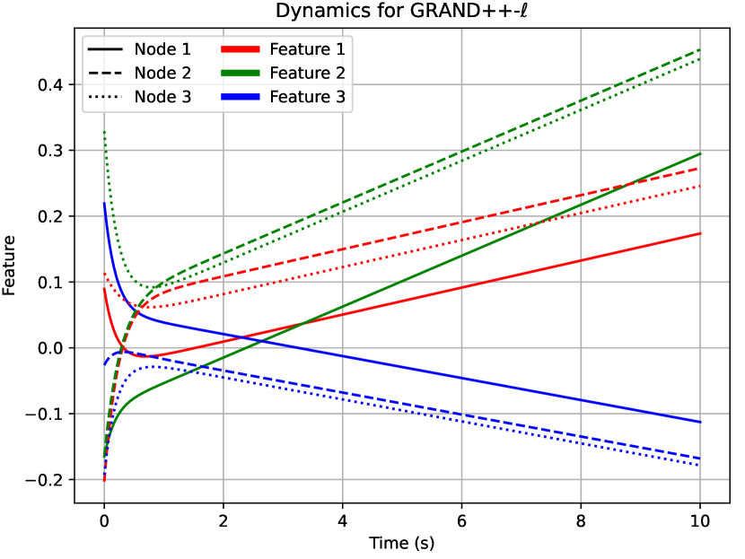
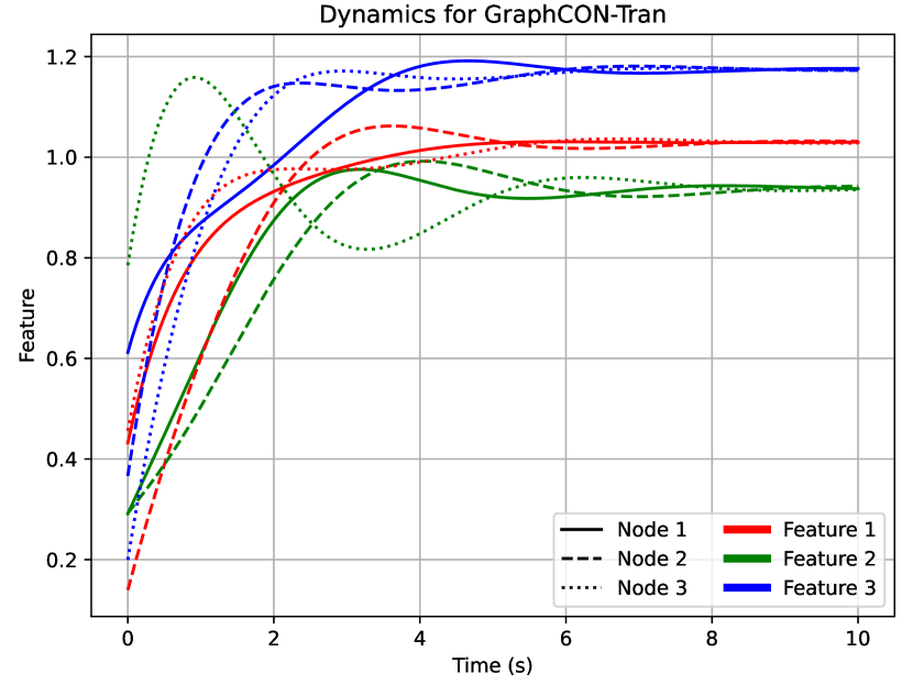
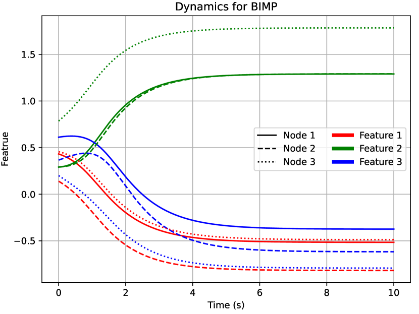
In right side of Figure 3, we present the simulated result for these four methods. We observe that features in GRAND- (upper left) quickly converge to the same values. In GraphCON-Tran (lower left), features also converge to the same but at slower speed rate due to its damping term resisting to the changes. Features in GRAND++- (upper right) remain a fixed difference between nodes after , but this difference get ignorable over time, ultimately leading to feature similarity. In contract, BIMP keeps distinct features throughout and mitigates the oversmoothing.
| Model | Texas | Wisconsin | Cornell |
| Homophily level | 0.11 | 0.21 | 0.30 |
| BIMP (ours) | 82.164.06 | 85.293.42 | 77.133.38 |
| GRAND- | 74.595.43 | 82.753.90 | 70.006.22 |
| GraphCON-GCN | 80.544.49 | 84.792.51 | 74.053.24 |
| KuramotoGNN | 81.814.36 | 85.094.42 | 76.022.77 |
D.2 Experiment on heterophilic datasets
We have evaluated our model on homophilic datasets in main paper, which holds the assumption that edges tend to connect similar nodes. However, many GNN models struggle with low accuracy on heterophilic datasets, where this assumption no longer holds. We deploy our BIMP model on three heterophilic datasets: Texas, Wisconsin, and Cornell from the CMU WebKB (Craven et al., 1998) project. BIMP demonstrates competitive performance while maintaining low computational complexity.
Table 7 lists the classification accuracy of BIMP and other continuous-depth GNNs on these heterophilic datasets. For all benchmarks, we run 10 fixed splits for each dataset with 20 random seeds for each split on work stations with an Intel Xeon Gold 5220R 24 core CPU, an Nvidia A6000 GPUs, and 256GB of RAM. The hyperparameters for BIMP are searched by Ray Tune process with 200 random trails.
Our BIMP model outperforms baselines in all datasets, illustrating its improved performance on heterophilic datasets.