Pareto-frontier Entropy Search with
Variational Lower Bound Maximization

Abstract

This study considers multi-objective Bayesian optimization (MOBO) through the information gain of the Pareto-frontier. To calculate the information gain, a predictive distribution conditioned on the Pareto-frontier plays a key role, which is defined as a distribution truncated by the Pareto-frontier. However, it is usually impossible to obtain the entire Pareto-frontier in a continuous domain, and therefore, the complete truncation cannot be known. We consider an approximation of the truncate distribution by using a mixture distribution consisting of two possible approximate truncation obtainable from a subset of the Pareto-frontier, which we call over- and under-truncation. Since the optimal balance of the mixture is unknown beforehand, we propose optimizing the balancing coefficient through the variational lower bound maximization framework, by which the approximation error of the information gain can be minimized. Our empirical evaluation demonstrates the effectiveness of the proposed method particularly when the number of objective functions is large.

1 Introduction

Multi-objective optimization (MOO) of black-box functions is ubiquitous in a variety of fields such as materials science, engineering, drug design, and AutoML. Evolutionary algorithms have been classically studied for MOO, but they require a large number of function evaluations, which is often difficult for practical problems. On the other hand, Bayesian optimization (BO) based approaches to MOO, which use a probabilistic surrogate model (typically, Gaussian process), have been widely studied recently (e.g., Knowles,, 2006; Emmerich,, 2005; Ponweiser et al.,, 2008; Belakaria et al.,, 2019; Suzuki et al.,, 2020; Qing et al.,, 2022; Tu et al.,, 2022).

This study focuses on multi-objective BO (MOBO) based on the information gain of the Pareto-frontier. Since the optimal solution of an MOO problem is not unique in general, the optimal values are represented as a set of output vectors, called the Pareto-frontier ${\cal F}^{*}$. Pareto-frontier entropy search (PFES) (Suzuki et al.,, 2020) considers the mutual-information between the Pareto-frontier and a candidate point as an acquisition function of MOBO. The effectiveness of the basic idea of PFES has been repeatedly shown (Qing et al.,, 2022; Tu et al.,, 2022).

In the information theoretic approaches considering the information of the Pareto-frontier (Suzuki et al.,, 2020; Qing et al.,, 2022; Tu et al.,, 2022), the predictive distribution given the Pareto-frontier $p(\boldsymbol{f}(\boldsymbol{x})\mid{\cal F}^{*})$ plays a key role in the information evaluation, where $\boldsymbol{f}(\boldsymbol{x})$ is a vector of objective function values at the input $\boldsymbol{x}$. In this distribution, $\boldsymbol{f}(\boldsymbol{x})$ cannot be better than ${\cal F}^{*}$ because ${\cal F}^{*}$ should be the Pareto-frontier. Therefore, $p(\boldsymbol{f}(\boldsymbol{x})\mid{\cal F}^{*})$ becomes a truncated distribution (see Fig. 1(a) for which details will be discussed in Section 3.2). However, it is practically impossible to obtain the entire ${\cal F}^{*}$ in a continuous space, and we only obtain a finite size subset ${\cal F}^{*}_{S}\subseteq{\cal F}^{*}$ (red stars in Fig. 1(a)). This means that the exact truncation by ${\cal F}^{*}$ shown in Fig. 1(a) cannot be calculated. To avoid this issue, all the existing studies use approximations based on an overly truncated distribution created by ${\cal F}^{*}_{S}$ (Fig. 1(d)). A drawback of this approach is that the effect of truncation by ${\cal F}^{*}$ on $\boldsymbol{f}(\boldsymbol{x})$ is always estimated stronger than the true truncation, because of which we call it over truncation.

In this study, we introduce the variational lower bound maximization approach into the mutual information (MI) estimation of information theoretic MOBO, which is called Pareto-frontier Entropy search with Variational lower bound maximization (PFEV). In addition to the conventional over truncation, we also consider a conservative approach, called under truncation (shown as Fig. 1(c)). The under truncation estimates the effect of truncation by ${\cal F}^{*}$ weaker than the true truncation. Therefore, to balance two opposite approaches, we combine the over and the under truncation in such a way that a mixture of them (Fig. 1(e)) defines a variational distribution of the MI approximation. We show that the mixture weight can be optimized through the variational lower bound maximization. This means that the optimal balance of the over and the under truncation can be determined so that the MI approximation error is minimized.

Our contribution is summarized as follows:

• PFEV is the first approach to continuous space MOBO that is based on a general lower bound of MI (existing work only shows a lower bound under a restrictive condition of two objective problems, for which we discuss in Section 4).

• We newly introduce an under truncation approximation for $p(\boldsymbol{f}(\boldsymbol{x})\mid{\cal F}^{*})$. Further, we define variational distribution as a mixture of distributions with the over and the under truncation, and show how to optimize the mixture weight.

• We also discuss properties and extensions of PFEV. For our MI lower bound, its relation with PI (probability of improvement) and a Monte-Carlo approximation are derived. We further discuss several extended settings such as parallel querying.

• Through empirical evaluation on Gaussian process generated and benchmark functions, we demonstrate effectiveness of PFEV. We empirically observed that PFEV shows a particular difference from existing over truncation based methods when output dimension $\geq 3$, in which the difference of two truncation becomes more apparent.

2 Multi-Objective Optimization and Gaussian Process Model

We consider Bayesian optimization (BO) for a multi-objective optimization (MOO) problem of maximizing $L\geq 2$ objective functions $f^{l}:{\cal X}\rightarrow\mathbb{R}$ $(l=1,\ldots,L)$, where ${\cal X}\subseteq\mathbb{R}^{d}$ is an input space. Let $\boldsymbol{f}_{\boldsymbol{x}}\coloneqq(f^{1}_{\boldsymbol{x}},\ldots,f^{L}_{\boldsymbol{x}})^{\top}$, where $f^{l}_{\boldsymbol{x}}\coloneqq f^{l}(\boldsymbol{x})$. The optimal solutions of MOO are characterized by the Parato optimality. For given $\boldsymbol{f}_{\boldsymbol{x}}$ and $\boldsymbol{f}_{\boldsymbol{x}^{\prime}}$, if $f^{l}_{\boldsymbol{x}}\geq f^{l}_{\boldsymbol{x}^{\prime}}$ for $\forall l\in\{1,\ldots,L\}$ and there exists $l$ that satisfies $f^{l}_{\boldsymbol{x}}>f^{l}_{\boldsymbol{x}^{\prime}}$, then “$\boldsymbol{f}_{\boldsymbol{x}}$ dominates $\boldsymbol{f}_{\boldsymbol{x}^{\prime}}$”, written as $\boldsymbol{f}_{\boldsymbol{x}}\succ\boldsymbol{f}_{\boldsymbol{x}^{\prime}}$. When $\boldsymbol{f}_{\boldsymbol{x}}$ is not dominated by any other $\boldsymbol{f}_{\boldsymbol{x}^{\prime}}$, then $\boldsymbol{f}_{\boldsymbol{x}}$ is Pareto optimal. The Pareto-frontier ${\cal F}^{*}$ is a set of Pareto optimal $\boldsymbol{f}_{\boldsymbol{x}}$ that can be defined as ${\cal F}^{*}\coloneqq\{\boldsymbol{f}_{\boldsymbol{x}}\in{\cal F}_{{\cal X}}\mid\boldsymbol{f}_{\boldsymbol{x}^{\prime}}\not\succ\boldsymbol{f}_{\boldsymbol{x}},\forall\boldsymbol{f}_{\boldsymbol{x}^{\prime}}\in{\cal F}_{{\cal X}}\}$, where ${\cal F}_{{\cal X}}\coloneqq\{\boldsymbol{f}_{\boldsymbol{x}}\in\mathbb{R}^{L}\mid\forall\boldsymbol{x}\in{\cal X}\}$.

Each objective function is represented by the Gaussian process (GP) regression. The observation of the $l$-th objective function is $y_{i}^{l}=f^{l}_{\boldsymbol{x}_{i}}+\varepsilon$, where $\varepsilon\sim{\cal N}(0,\sigma^{2}_{\rm noise})$. The training dataset with $n$ observations is written as ${\cal D}\coloneqq\{(\boldsymbol{x}_{i},\boldsymbol{y}_{i})\}_{i=1}^{n}$, where $\boldsymbol{y}_{i}=(y_{i}^{1},\ldots,y_{i}^{L})^{\top}$. We use independent $L$ GPs with a kernel function $k(\boldsymbol{x},\boldsymbol{x}^{\prime})$. Let $\boldsymbol{k}(\boldsymbol{x})\coloneqq(k(\boldsymbol{x},\boldsymbol{x}_{1}),\ldots,k(\boldsymbol{x}_{,}\boldsymbol{x}_{n}))^{\top}$, $\boldsymbol{y}^{l}\coloneqq(y_{1}^{l},\ldots,y_{n}^{l})^{\top}$, and $\boldsymbol{K}$ be a matrix whose $(i,j)$ element is $k(\boldsymbol{x}_{i},\boldsymbol{x}_{j})$. The posterior $p(f^{l}_{\boldsymbol{x}}\mid{\cal D})$ of the $l$-th GP (with $0$ prior mean) is written as ${\cal N}(\mu_{l}(\boldsymbol{x}),\sigma^{2}_{l}(\boldsymbol{x}))$, where $\mu_{l}(\boldsymbol{x})=\boldsymbol{k}(\boldsymbol{x})^{\top}\left(\boldsymbol{K}+\sigma^{2}_{\rm noise}\boldsymbol{I}\right)^{-1}\boldsymbol{y}^{l}$ and $\sigma^{2}_{l}(\boldsymbol{x})=k(\boldsymbol{x},\boldsymbol{x})-\boldsymbol{k}(\boldsymbol{x})^{\top}\left(\boldsymbol{K}+\sigma^{2}_{\rm noise}\boldsymbol{I}\right)^{-1}\boldsymbol{k}(\boldsymbol{x})$. From independence, we have $p(\boldsymbol{f}_{\boldsymbol{x}}\mid{\cal D})=\prod_{l\in[L]}p(f^{l}_{\boldsymbol{x}}\mid{\cal D})$. For notational brevity, conditioning on ${\cal D}$ is omitted (e.g., $p(\boldsymbol{f}_{\boldsymbol{x}}\mid{\cal D})$ is written as $p(\boldsymbol{f}_{\boldsymbol{x}})$).

3 Pareto-frontier Entropy Search with Variation Lower Bound Maximization

We consider multi-objective Bayesian optimization (MOBO) based on mutual information ${\rm MI}(\boldsymbol{f}_{\boldsymbol{x}};{\cal F}^{*})$ between an objective function value $\boldsymbol{f}_{\boldsymbol{x}}$ and the Pareto-frontier ${\cal F}^{*}$ (Note that, throughout the paper, ${\cal F}^{*}$ is a random variable determined via the predictive distribution of $\boldsymbol{f}_{\boldsymbol{x}}$). An intuition behind this criterion is to select $\boldsymbol{x}$ that provides the maximum information gain of the Pareto-frontier ${\cal F}^{*}$. The effectiveness of this approach is shown by (Suzuki et al.,, 2020), but it is known that accurate evaluation of ${\rm MI}(\boldsymbol{f}_{\boldsymbol{x}};{\cal F}^{*})$ is difficult. Our proposed method is the first method introducing the variational lower bound maximization to evaluate ${\rm MI}(\boldsymbol{f}_{\boldsymbol{x}};{\cal F}^{*})$. We call our proposed method Pareto-frontier Entropy search with Variational lower bound maximization (PFEV).

3.1 Lower Bound of Mutual Information

A lower bound $L(\boldsymbol{x})$ of ${\rm MI}(\boldsymbol{f}_{\boldsymbol{x}};{\cal F}^{*})$ can be derived as

$$\mathrm{MI}(\boldsymbol{f}_{\boldsymbol{x}};{\cal F}^{*})$$

$$=\int p({\cal F}^{*})\int p(\boldsymbol{f}_{\boldsymbol{x}}\mid{\cal F}^{*})\log\frac{p({\boldsymbol{f}_{\boldsymbol{x}}}\mid{\cal F}^{*})}{p({\boldsymbol{f}_{\boldsymbol{x}}})}\mathrm{d}\boldsymbol{f}_{\boldsymbol{x}}\mathrm{d}{\cal F}^{*}$$

$$=\int p({\cal F}^{*})\left[\int p(\boldsymbol{f}_{\boldsymbol{x}}\mid{\cal F}^{*})\log\frac{q(\boldsymbol{f}_{\boldsymbol{x}}\mid{\cal F}^{*})}{p(\boldsymbol{f}_{\boldsymbol{x}})}\mathrm{d}\boldsymbol{f}_{\boldsymbol{x}}\right.$$

$$\qquad\left.+D_{\mathrm{KL}}\left(p(\boldsymbol{f}_{\boldsymbol{x}}\mid{\cal F}^{*})\parallel q(\boldsymbol{f}_{\boldsymbol{x}}\mid{\cal F}^{*})\right)\right]\mathrm{d}{\cal F}^{*}$$

$$\geq\mathbb{E}_{{\cal F}^{*}}\left[\int p(\boldsymbol{f}_{\boldsymbol{x}}\mid{\cal F}^{*})\log\frac{q(\boldsymbol{f}_{\boldsymbol{x}}\mid{\cal F}^{*})}{p(\boldsymbol{f}_{\boldsymbol{x}})}\mathrm{d}\boldsymbol{f}_{\boldsymbol{x}}\right]$$

$$=\mathbb{E}_{{\cal F}^{*},\boldsymbol{f}_{\boldsymbol{x}}}\left[\log\frac{q(\boldsymbol{f}_{\boldsymbol{x}}\mid{\cal F}^{*})}{p(\boldsymbol{f}_{\boldsymbol{x}})}\right]\eqqcolon L(\boldsymbol{x}),$$ (1)

where $D_{\mathrm{KL}}$ is Kullback-Leibler (KL) divergence, and $q(\boldsymbol{f}_{\boldsymbol{x}}\mid{\cal F}^{*})$ is a density function called a variational distribution. A similar lower bound was first derived in the context of constrained BO (Takeno et al.,, 2022). This lower bound holds for any distribution $q(\boldsymbol{f}_{\boldsymbol{x}}\mid{\cal F}^{*})$ that satisfies the following support condition:

$$\mathrm{supp}(q(\boldsymbol{f}_{\boldsymbol{x}}\mid{\cal F}^{*}))\supseteq\mathrm{supp}(p({\boldsymbol{f}_{\boldsymbol{x}}}\mid{\cal F}^{*})),$$ (2)

where $\mathrm{supp}$ is a set of non-zero point of a given density, defined as $\mathrm{supp}(p(\boldsymbol{f}\mid{\cal F}^{*}))=\{\boldsymbol{f}\in\mathbb{R}^{L}\mid p(\boldsymbol{f}\mid{\cal F}^{*})\neq 0\}$. In addition to this condition, the lower bound $L(\boldsymbol{x})$ is derived by using a convention $0\log 0=0$ (Cover and Thomas,, 2006). We call the condition (2) variational distribution condition (VDC). Note that if VDC is not satisfied, $L(\boldsymbol{x})$ is not defined because of $\log 0$.

3.2 Variational Lower Bound Maximization by Combining Over and Under Truncation

If $q(\boldsymbol{f}_{\boldsymbol{x}}\mid{\cal F}^{*})=p(\boldsymbol{f}_{\boldsymbol{x}}\mid{\cal F}^{*})$, the lower bound $L(\boldsymbol{x})$ is equal to $\mathrm{MI}(\boldsymbol{f}_{\boldsymbol{x}};{\cal F}^{*})$. However, the analytical representation of $p(\boldsymbol{f}_{\boldsymbol{x}}\mid{\cal F}^{*})$ is not known. This stems from a common well-known difficulty of information-theoretic BO, and effectiveness of the truncated distribution based approximation has been repeatedly shown (e.g., Wang and Jegelka,, 2017; Takeno et al.,, 2020; Perrone et al.,, 2019; Suzuki et al.,, 2020) not only for MOBO, but also for a variety contexts of BO problems (such as standard single objective problems, constraint problems, and multi-fidelity problems).

Define $\boldsymbol{f}\preceq{\cal F}^{*}$ as that $\boldsymbol{f}$ is dominated by or equal to at least one element in ${\cal F}^{*}$. The truncation-based approximation replaces the condition in $p(\boldsymbol{f}_{\boldsymbol{x}}\mid{\cal F}^{*})$ with $\boldsymbol{f}_{\boldsymbol{x}}\preceq{\cal F}^{*}$, by which we obtain $q(\boldsymbol{f}_{\boldsymbol{x}}\mid{\cal F}^{*})=p(\boldsymbol{f}_{\boldsymbol{x}}\mid\boldsymbol{f}_{\boldsymbol{x}}\preceq{\cal F}^{*})$:

$$q(\boldsymbol{f}_{\boldsymbol{x}}\mid{\cal F}^{*})=\begin{cases}p(\boldsymbol{f}_{\boldsymbol{x}})/Z^{{\cal F}^{*}}(\boldsymbol{x})&\text{ if }\boldsymbol{f}_{\boldsymbol{x}}\in{\cal A}^{{\cal F}^{*}},\\ 0&\text{ otherwise, }\end{cases}$$

where ${\cal A}^{{\cal F}^{*}}\coloneqq\{\boldsymbol{f}\in\mathbb{R}^{L}\mid\boldsymbol{f}\preceq\boldsymbol{f}^{\prime},\exists\boldsymbol{f}^{\prime}\in{\cal F}^{*}\}$ and $Z^{{\cal F}^{*}}(\boldsymbol{x})\coloneqq p(\boldsymbol{f}_{\boldsymbol{x}}\in{\cal A}^{{\cal F}^{*}})$ is a normalization constant. As shown in Fig. 1(a), $q(\boldsymbol{f}_{\boldsymbol{x}}\mid{\cal F}^{*})$ is a truncated normal distribution in which only the region dominated by ${\cal F}^{*}$ remains. Suzuki et al., (2020) call this distribution PFTN (Pareto-Frontier Truncated Normal distribution). PFTN is derived by the fact that if ${\cal F}^{*}$ is given, any $\boldsymbol{f}_{\boldsymbol{x}}$ dominating ${\cal F}^{*}$ cannot exist. However, ${\cal F}^{*}$ cannot be obtained in practice in the continuous domain, and we only obtain limited discrete points, such as those indicated by the red star points in Fig. 1(a). A subset of ${\cal F}^{*}$ defined by these discrete points is written as ${\cal F}^{*}_{S}\subseteq{\cal F}^{*}$ (We discuss how to calculate ${\cal F}^{*}_{S}$ in Section 3.3). In this study, we consider combining two truncated distributions derived by ${\cal F}^{*}_{S}$, instead of using ${\cal F}^{*}$ that is not obtainable.

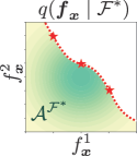
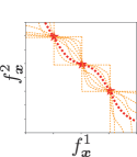
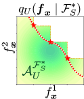
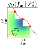
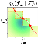
Figure 1: (a) Predictive distribution truncated by ${\cal F}^{*}$. (b) Examples of possible truncation given ${\cal F}^{*}_{S}$. (c) Under truncation based on $\tilde{{\cal F}}^{*}_{S}$. (d) Over truncation based on $\tilde{{\cal F}}^{*}_{S}$. (e) Mixture of $q_{U}(\boldsymbol{f}_{\boldsymbol{x}}\mid\tilde{{\cal F}}^{*}_{S})$ and $q_{O}(\boldsymbol{f}_{\boldsymbol{x}}\mid\tilde{{\cal F}}^{*}_{S})$.

In Fig. 1(b), the orange dashed lines are examples of possible truncation behind ${\cal F}_{S}^{*}$ and the red dot line is the true ${\cal F}^{*}$, which is unknown. The first truncated distribution is based on the most conservative truncation show in Fig. 1(c). This truncation is defined by removing “the region that dominates ${\cal F}^{*}_{S}$” (any point that dominates ${\cal F}^{*}_{S}$ cannot exist). The remaining region is written as ${\cal A}_{U}^{{\cal F}^{*}_{S}}\coloneqq\mathbb{R}^{L}\setminus\{\boldsymbol{f}\in\mathbb{R}^{L}\mid\boldsymbol{f}^{\prime}\preceq\boldsymbol{f},\exists\boldsymbol{f}^{\prime}\in{\cal F}^{*}_{S}\}$. The resulting truncated normal distribution is

$$q_{U}(\boldsymbol{f}_{\boldsymbol{x}}\mid{\cal F}^{*}_{S})\coloneqq\begin{cases}p(\boldsymbol{f}_{\boldsymbol{x}})/Z_{U}^{{\cal F}^{*}_{S}}(\boldsymbol{x})&\text{ if }\boldsymbol{f}_{\boldsymbol{x}}\in{\cal A}_{U}^{{\cal F}^{*}_{S}},\\ 0&\text{ otherwise, }\end{cases}$$

where $Z_{U}^{{\cal F}^{*}_{S}}(\boldsymbol{x})\coloneqq p(\boldsymbol{f}_{\boldsymbol{x}}\in{\cal A}_{U}^{{\cal F}^{*}_{S}})$. We call this distribution PFTN-U (PFTN with under truncation). PFTN-U has a larger support $\mathrm{supp}(q_{U}(\boldsymbol{f}_{\boldsymbol{x}}\mid{\cal F}^{*}_{S}))\supseteq\mathrm{supp}(p({\boldsymbol{f}_{\boldsymbol{x}}}\mid{\cal F}^{*}))$, and thus, VDC is satisfied. This truncation is conservative in the sense that the region where the density function becomes zero is smaller than $q(\boldsymbol{f}_{\boldsymbol{x}}\mid{\cal F}^{*})$, by which it underestimates the effect of the condition $\boldsymbol{f}_{\boldsymbol{x}}\preceq{\cal F}^{*}$ on $\boldsymbol{f}_{\boldsymbol{x}}$.

The second truncated distribution is based on the over truncation shown in Fig 1(d). This is “the region dominated by ${\cal F}^{*}_{S}$”, defined as ${\cal A}_{O}^{{\cal F}^{*}_{S}}\coloneqq\{\boldsymbol{f}\in\mathbb{R}^{L}\mid\boldsymbol{f}\preceq\boldsymbol{f}^{\prime},\exists\boldsymbol{f}^{\prime}\in{\cal F}^{*}_{S}\}$. The resulting truncated normal distribution is

$$q_{O}(\boldsymbol{f}_{\boldsymbol{x}}\mid{\cal F}^{*}_{S})\coloneqq\begin{cases}p(\boldsymbol{f}_{\boldsymbol{x}})/Z_{O}^{{\cal F}^{*}_{S}}(\boldsymbol{x})&\text{ if }\boldsymbol{f}_{\boldsymbol{x}}\in{\cal A}_{O}^{{\cal F}^{*}_{S}},\\ 0&\text{ otherwise, }\end{cases}$$

where $Z_{O}^{{\cal F}^{*}_{S}}(\boldsymbol{x})\coloneqq p(\boldsymbol{f}_{\boldsymbol{x}}\in{\cal A}_{O}^{{\cal F}^{*}_{S}})$. In contrast to $q_{U}$, $q_{O}$ overly truncates the distribution in the sense that the region where the density function value becomes zero is larger than $q(\boldsymbol{f}_{\boldsymbol{x}}\mid{\cal F}^{*})$, by which it overestimates the effect of the condition $\boldsymbol{f}_{\boldsymbol{x}}\preceq{\cal F}^{*}$ on $\boldsymbol{f}_{\boldsymbol{x}}$. We call this distribution PFTN-O (PFTN with over truncation). It is important to note that PFTN-O may not satisfy VDC (2) because $\mathrm{supp}(q_{O}(\boldsymbol{f}_{\boldsymbol{x}}\mid{\cal F}^{*}_{S}))\subseteq\mathrm{supp}(p({\boldsymbol{f}_{\boldsymbol{x}}}\mid{\cal F}^{*}))$,

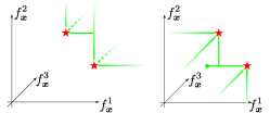
Figure 2: An example of truncation in three dimensional output space. The resulting truncate regions have a large difference.

As we already discussed, $q_{O}$ and $q_{U}$ over and under estimates the truncation by the true ${\cal F}^{*}$. Therefore, instead of using one of them, we consider the mixture defined as follows:

$$q_{\lambda}(\boldsymbol{f}_{\boldsymbol{x}}\mid{\cal F}^{*}_{S})=\lambda q_{U}(\boldsymbol{f}_{\boldsymbol{x}}\mid{\cal F}^{*}_{S})+(1-\lambda)q_{O}(\boldsymbol{f}_{\boldsymbol{x}}\mid{\cal F}^{*}_{S}),$$

$$=\begin{cases}\left(\frac{\lambda}{Z_{U}^{{\cal F}^{*}_{S}}(\boldsymbol{x})}+\frac{1-\lambda}{Z_{O}^{{\cal F}^{*}_{S}}(\boldsymbol{x})}\right)p(\boldsymbol{f}_{\boldsymbol{x}})&\text{ if }\boldsymbol{f}_{\boldsymbol{x}}\in{\cal A}_{O}^{{\cal F}^{*}_{S}},\\ \lambda p(\boldsymbol{f}_{\boldsymbol{x}})/Z_{U}^{{\cal F}^{*}_{S}}(\boldsymbol{x})&\text{ if }\boldsymbol{f}_{\boldsymbol{x}}\in{\cal A}_{U\setminus O}^{{\cal F}^{*}_{S}},\\ 0&\text{ otherwise, }\end{cases}$$ (3)

where ${\cal A}_{U\setminus O}^{{\cal F}^{*}_{S}}\coloneqq{\cal A}_{U}^{{\cal F}^{*}_{S}}\setminus{\cal A}_{O}^{{\cal F}^{*}_{S}}$, and $\lambda\in(0,1]$ is a weight of the mixture. Because of $\lambda\neq 0$, we have $\mathrm{supp}(q_{\lambda}(\boldsymbol{f}_{\boldsymbol{x}}\mid{\cal F}^{*}_{S}))\supseteq\mathrm{supp}(p({\boldsymbol{f}_{\boldsymbol{x}}}\mid{\cal F}^{*}))$, meaning that the mixture satisfies VDC. Figure 1(e) shows an example of the mixture. The effect of PFTN-U and PFTN-O can be controlled by $\lambda$. In the 2D illustration in Fig. 1, the difference between the two truncation might appear small. However, as shown in Fig. 2, in three or more dimensions, the two truncation are significantly different, obviously. Therefore, we conjecture that the balance of them can have a strong effect particularly for problems with $L\geq 3$.

By substituting $q_{\lambda}(\boldsymbol{f}_{\boldsymbol{x}}\mid{\cal F}^{*}_{S})$ into $L(\boldsymbol{x})$, we define $L(\boldsymbol{x},\lambda)$ as

$$L(\boldsymbol{x},\lambda)$$

$$=\mathbb{E}_{{\cal F}^{*},\boldsymbol{f}_{\boldsymbol{x}}}\left[\log\left(\frac{\lambda q_{U}(\boldsymbol{f}_{\boldsymbol{x}}\mid{\cal F}^{*}_{S})+(1-\lambda)q_{O}(\boldsymbol{f}_{\boldsymbol{x}}\mid{\cal F}^{*}_{S})}{p(\boldsymbol{f}_{\boldsymbol{x}})}\right)\right]$$

$$=\mathbb{E}_{{\cal F}^{*},\boldsymbol{f}_{\boldsymbol{x}}}\bigl{[}\log\bigl{\{}\zeta_{\lambda}^{{\cal F}^{*}_{S}}(\boldsymbol{x})\mathbb{I}(\boldsymbol{f}_{\boldsymbol{x}}\in{\cal A}_{O}^{{\cal F}^{*}_{S}})$$

$$\qquad\qquad\qquad+\eta_{\lambda}^{{\cal F}^{*}_{S}}(\boldsymbol{x})\mathbb{I}(\boldsymbol{f}_{\boldsymbol{x}}\in{\cal A}_{U\setminus O}^{{\cal F}^{*}_{S}})\bigr{\}}\bigr{]},$$ (4)

where $\zeta_{\lambda}^{{\cal F}^{*}_{S}}(\boldsymbol{x})=\frac{\lambda}{Z_{U}^{{\cal F}^{*}_{S}}(\boldsymbol{x})}+\frac{1-\lambda}{Z_{O}^{{\cal F}^{*}_{S}}(\boldsymbol{x})}$, $\eta_{\lambda}^{{\cal F}^{*}_{S}}(\boldsymbol{x})=\frac{\lambda}{Z_{U}^{{\cal F}^{*}_{S}}(\boldsymbol{x})}$, and $\mathbb{I}$ is the indicator function. Importantly, the weight parameter $\lambda$ can be estimated by maximizing the lower bound:

$$\max_{\lambda\in(0,1]}L(\boldsymbol{x},\lambda)$$ (5)

This maximization implies the following property, which is a well-known advantage of the variational lower bound maximization (Bishop and Bishop,, 2023):

Remarks 3.1.

From (1),

$$\mathrm{MI}(\boldsymbol{f}_{\boldsymbol{x}};{\cal F}^{*})= L(\boldsymbol{x},\lambda)$$

$$+\mathbb{E}_{{\cal F}^{*}}\left[D_{\mathrm{KL}}\left(p(\boldsymbol{f}_{\boldsymbol{x}}\mid{\cal F}^{*})\parallel q_{\lambda}(\boldsymbol{f}_{\boldsymbol{x}}\mid{\cal F}^{*})\right)\right].$$

Therefore, (5) is equivalent to

$$\min_{\lambda\in(0,1]}\mathbb{E}_{{\cal F}^{*}}\left[D_{\mathrm{KL}}\left(p(\boldsymbol{f}_{\boldsymbol{x}}\mid{\cal F}^{*})\parallel q_{\lambda}(\boldsymbol{f}_{\boldsymbol{x}}\mid{\cal F}^{*})\right)\right].$$

As a result, (5) can be seen as the minimization of difference between true $p(\boldsymbol{f}_{\boldsymbol{x}}\mid{\cal F}^{*})$ and $q_{\lambda}$.

Further, we have the following property:

Remarks 3.2.

(5) can be bounded from below (the proof is in Appendix A):

$$\max_{\lambda\in(0,1]}L(\boldsymbol{x},\lambda)\geq\mathbb{E}_{{\cal F}^{*}}\left[p(\boldsymbol{f}_{\boldsymbol{x}}\notin{\cal A}_{U}^{{\cal F}_{S}^{*}})\right]>0.$$

$p(\boldsymbol{f}_{\boldsymbol{x}}\notin{\cal A}_{U}^{{\cal F}_{S}^{*}})$ can be seen as the probability of improvement (PI) from the region ${\cal A}_{U}^{{\cal F}_{S}^{*}}$, from which positivity of (5) is also directly derived.

While MI has a trivial lower bound $0$ in general, this remark guarantees that (5) is a larger lower bound than this trivial bound. Further, we can also see that if the candidate $\boldsymbol{x}$ is a promising in a sense of PI, (5) should have substantially larger value than $0$.

As a result, the selection of $\boldsymbol{x}$ is formulated as

$$\max_{\boldsymbol{x},\lambda\in(0,1]}L(\boldsymbol{x},\lambda),$$

in which $\boldsymbol{x}$ and $\lambda$ can be simultaneously optimized ($d+1$ dimensional maximization).

3.3 Computations

We employ the Monte-Carlo (MC) estimation to calculate the expectation in $L(\boldsymbol{x},\lambda)$:

$$L(\boldsymbol{x},\lambda) \approx\frac{1}{K}\sum_{(\tilde{{\cal F}}^{*}_{S},\tilde{\boldsymbol{f}})\in F}\log\left\{\zeta_{\lambda}^{\tilde{{\cal F}}^{*}_{S}}(\boldsymbol{x})\mathbb{I}(\tilde{\boldsymbol{f}_{\boldsymbol{x}}}\in{\cal A}_{O}^{\tilde{{\cal F}}^{*}_{S}})\right.$$

$$\qquad\qquad\qquad+\left.\eta_{\lambda}^{\tilde{{\cal F}}^{*}_{S}}(\boldsymbol{x})\mathbb{I}(\tilde{\boldsymbol{f}}_{\boldsymbol{x}}\in{\cal A}_{U\setminus O}^{\tilde{{\cal F}}^{*}_{S}})\right\},$$ (6)

where $F$ is a set of sampled pairs of $({\cal F}^{*}_{S},\boldsymbol{f})$, for which a sample pair is denoted as $(\tilde{{\cal F}}^{*}_{S},\tilde{\boldsymbol{f}})$, and $K=|F|$ is the number of samplings. Henceforth, variables with ‘ $\tilde{}$ ’ indicate sampled values. For ${\cal F}^{*}_{S}$, the same sampling strategy can be used as existing information-theoretic MOBO (Suzuki et al.,, 2020; Hernandez-Lobato et al.,, 2016), in which a sample path $\tilde{f}^{l}$ is approximately generated by using random feature map (RFM) (Rahimi and Recht,, 2008). We obtain ${\cal F}^{*}_{S}$ by solving the MOO maximizing sampled $\tilde{f}^{l}(\boldsymbol{x})$ for $l=1,\ldots,L$. This maximization can be performed by general MOO solvers such as well-known NSGA-II (Deb et al.,, 2002). In the case of NSGA-II, $|{\cal F}^{*}_{S}|$ can be specified, typically less than $100$. Computations of $Z_{O}^{\tilde{{\cal F}}^{*}_{S}}$ and $Z_{U}^{\tilde{{\cal F}}^{*}_{S}}$ can be easily performed by the cell (hyper-rectangle) decomposition-based approach as shown by (Suzuki et al.,, 2020) for which details are in Appendix B. This decomposition is only required once for each iteration of BO because it is common for all candidate $\boldsymbol{x}$.

We also consider another way to numerically approximate $L(\boldsymbol{x},\lambda)$ based on the following transformation:

$$L(\boldsymbol{x},\lambda)$$

$$=\!\mathbb{E}_{{\cal F}^{*},\boldsymbol{f}_{\boldsymbol{x}}}\!\left[\mathbb{I}(\boldsymbol{f}_{\boldsymbol{x}}\in{\cal A}_{O}^{{\cal F}^{*}_{S}})\log\zeta_{\lambda}^{\tilde{{\cal F}}^{*}_{S}}(\boldsymbol{x})\!+\!\mathbb{I}(\boldsymbol{f}_{\boldsymbol{x}}\in{\cal A}_{U\setminus O}^{{\cal F}^{*}_{S}})\log\eta_{\lambda}^{\tilde{{\cal F}}^{*}_{S}}(\boldsymbol{x})\right]$$

$$=\mathbb{E}_{{\cal F}^{*}}\left[p(\boldsymbol{f}_{\boldsymbol{x}}\in{\cal A}_{O}^{{\cal F}^{*}_{S}}\mid{\cal F}^{*})\log\zeta_{\lambda}^{\tilde{{\cal F}}^{*}_{S}}(\boldsymbol{x})\right.$$

$$\qquad\qquad\qquad\left.+p(\boldsymbol{f}_{\boldsymbol{x}}\in{\cal A}_{U\setminus O}^{{\cal F}^{*}_{S}}\mid{\cal F}^{*})\log\eta_{\lambda}^{\tilde{{\cal F}}^{*}_{S}}(\boldsymbol{x})\right]$$

$$\approx\frac{1}{K}\sum_{(\tilde{{\cal F}}^{*}_{S},\tilde{\boldsymbol{f}})\in F}p(\boldsymbol{f}_{\boldsymbol{x}}\in{\cal A}_{O}^{\tilde{{\cal F}}^{*}_{S}}\mid\tilde{{\cal F}}^{*})\log\zeta_{\lambda}^{\tilde{{\cal F}}^{*}_{S}}(\boldsymbol{x})$$

$$\qquad\qquad+p(\boldsymbol{f}_{\boldsymbol{x}}\in{\cal A}_{U\setminus O}^{\tilde{{\cal F}}^{*}_{S}}\mid\tilde{{\cal F}}^{*})\log\eta_{\lambda}^{\tilde{{\cal F}}^{*}_{S}}(\boldsymbol{x}).$$ (7)

Note that the second line is from $\mathbb{I}(\boldsymbol{f}_{\boldsymbol{x}}\in{\cal A}_{O}^{{\cal F}^{*}_{S}})=1-\mathbb{I}(\boldsymbol{f}_{\boldsymbol{x}}\in{\cal A}_{U\setminus O}^{{\cal F}^{*}_{S}})$, and the third line is obtained by replacing $\mathbb{E}_{{\cal F}^{*},\boldsymbol{f}_{\boldsymbol{x}}}$ with $\mathbb{E}_{{\cal F}^{*}}\mathbb{E}_{\boldsymbol{f}_{\boldsymbol{x}}\mid{\cal F}^{*}}$. Since (6) can be re-written as $\frac{1}{K}\sum_{(\tilde{{\cal F}}^{*}_{S},\tilde{\boldsymbol{f}})\in F}\mathbb{I}(\tilde{\boldsymbol{f}_{\boldsymbol{x}}}\in{\cal A}_{O}^{\tilde{{\cal F}}^{*}_{S}})\log\zeta_{\lambda}^{\tilde{{\cal F}}^{*}_{S}}(\boldsymbol{x})+\mathbb{I}(\tilde{\boldsymbol{f}}_{\boldsymbol{x}}\in{\cal A}_{U\setminus O}^{\tilde{{\cal F}}^{*}_{S}})\log\eta_{\lambda}^{\tilde{{\cal F}}^{*}_{S}}(\boldsymbol{x})$, by comparing this re-written expression with (7), we can interpret that (6) performs one sample approximations $p(\boldsymbol{f}_{\boldsymbol{x}}\in{\cal A}_{O}^{\tilde{{\cal F}}^{*}_{S}}\mid\tilde{{\cal F}}^{*})\approx\mathbb{I}(\tilde{\boldsymbol{f}}_{\boldsymbol{x}}\in{\cal A}_{O}^{\tilde{{\cal F}}^{*}_{S}})$ and $p(\boldsymbol{f}_{\boldsymbol{x}}\in{\cal A}_{U\setminus O}^{\tilde{{\cal F}}^{*}_{S}}\mid\tilde{{\cal F}}^{*})\approx\mathbb{I}(\tilde{\boldsymbol{f}}_{\boldsymbol{x}}\in{\cal A}_{U\setminus O}^{\tilde{{\cal F}}^{*}_{S}})$. We consider improving this approximations by introducing a prior knowledge about $p(\boldsymbol{f}_{\boldsymbol{x}}\in{\cal A}_{O}^{\tilde{{\cal F}}^{*}_{S}}\mid\tilde{{\cal F}}^{*})$ and $p(\boldsymbol{f}_{\boldsymbol{x}}\in{\cal A}_{U\setminus O}^{\tilde{{\cal F}}^{*}_{S}}\mid\tilde{{\cal F}}^{*})$.

Let $\theta\coloneqq p(\boldsymbol{f}_{\boldsymbol{x}}\in{\cal A}_{O}^{\tilde{{\cal F}}^{*}_{S}}\mid\tilde{{\cal F}}^{*})$. We use an approximation $\theta\approx p(\boldsymbol{f}_{\boldsymbol{x}}\in{\cal A}_{O}^{\tilde{{\cal F}}^{*}_{S}}\mid\boldsymbol{f}_{\boldsymbol{x}}\in{\cal A}_{U}^{\tilde{{\cal F}}^{*}_{S}})=Z_{O}^{\tilde{{\cal F}}^{*}_{S}}(\boldsymbol{x})/Z_{U}^{\tilde{{\cal F}}^{*}_{S}}(\boldsymbol{x})\eqqcolon\hat{p}$ as our prior knowledge. The approximation is replacement of the conditioning by $\tilde{{\cal F}}^{*}$ with the under truncation $\boldsymbol{f}_{\boldsymbol{x}}\in{\cal A}_{U}^{\tilde{{\cal F}}^{*}_{S}}$. Note that $Z_{O}^{\tilde{{\cal F}}^{*}_{S}}(\boldsymbol{x})$ and $Z_{U}^{\tilde{{\cal F}}^{*}_{S}}(\boldsymbol{x})$ are required even in the naïve MC (6), $\hat{p}$ can be obtained without additional computations. A prior distribution having the mode at $\hat{p}$ is introduced to estimate $\theta$. We use the beta distribution by which MAP (maximum a posteriori) becomes

$$\theta_{\mathrm{MAP}}(\boldsymbol{f}_{\boldsymbol{x}})=\frac{\hat{p}+\mathbb{I}(\boldsymbol{f}_{\boldsymbol{x}}\in{\cal A}_{O}^{\tilde{{\cal F}}^{*}_{S}})}{2}.$$

The detailed derivation is in Appendix D.1. $\theta_{\mathrm{MAP}}$ can be seen as an average of $\hat{p}$ and $\mathbb{I}(\boldsymbol{f}_{\boldsymbol{x}}\in{\cal A}_{O}^{\tilde{{\cal F}}^{*}_{S}})$.

As a result, we obtain

$$L(\boldsymbol{x},\lambda) \approx\frac{1}{K}\sum_{(\tilde{{\cal F}}^{*}_{S},\tilde{\boldsymbol{f}})\in F}\theta_{\mathrm{MAP}}(\tilde{\boldsymbol{f}}_{\boldsymbol{x}})\log\zeta_{\lambda}^{\tilde{{\cal F}}^{*}_{S}}(\boldsymbol{x})$$

$$+(1-\theta_{\mathrm{MAP}}(\tilde{\boldsymbol{f}}_{\boldsymbol{x}}))\log\eta_{\lambda}^{\tilde{{\cal F}}^{*}_{S}}(\boldsymbol{x})\eqqcolon\widehat{L}(\boldsymbol{x},\lambda).$$ (8)

We empirically observe that the estimation variance can be improved by the prior. Instead, the bias to $\hat{p}$ can occur, but because the number of samplings is usually small (our default setting is $K=10$ in the experiments, which is same as existing information-theoretic BO studies such as (Wang and Jegelka,, 2017)), variance reduction has a stronger benefit in practice. Further discussion on the accuracy of this estimator is in Appendix D.2 and D.3.

The procedure of PFEV is shown in Algorithm 1. Assume that we already have the posterior mean and variance of GPs. Then, computations of (8) is $O(KCL)$, where $C$ is the number of hyper-rectangle cells in the decomposition. For the cell decomposition, we employ the quick hyper-volume (QHV) algorithm (Russo and Francisco,, 2014) as indicated by (Suzuki et al.,, 2020). Sampling of $F$ requires $O(D^{3})$ for RFM with $D$ basis functions and the cost of NSGA-II is also required. We empirically see that, for small $L$, the computational cost of NSGA-II is dominant, and for large $L$, QHV becomes dominant, both of which are commonly required for several information-theoretic MOBO (Suzuki et al.,, 2020; Qing et al.,, 2022; Tu et al.,, 2022). Compared with them, the practical cost of the lower bound calculation in CalcPFEV of Algorithm 1 is often relatively small (see Appendix K.3 for detail). As discussed in the end of Section 3.2, the acquisition function maximization is formulated as $d+1$ dimensional optimization (line 10 of Algorithm). On the other hand, it is also possible to optimize $\lambda$ for each given $\boldsymbol{x}$ as an inner one dimensional optimization. In the later case, efficient computations can be performed by considering (8) (or (6)) is concave with respect to $\lambda$ (Details are in Appendix C).

Algorithm 1 Pseudo-code of PFEV

1: Function PFEV( Initial dataset ${\cal D}_{0}$ ):

2: for $t=0,\ldots,T$ do

3:  $F\leftarrow\{\}$

4:  for $k=1,\ldots,K$ do

5:   Generate a sample path $\tilde{\boldsymbol{f}}$ from the current posterior of $\boldsymbol{f}$

6:   Obtain $\tilde{{\cal F}}_{S}^{*}$ by applying NSGA-II to $\tilde{\boldsymbol{f}}_{\boldsymbol{x}}$

7:   Create cell-decomposition by QHV

8:   $F\leftarrow F\cup(\tilde{{\cal F}}_{S}^{*},\tilde{\boldsymbol{f}})$

9:  end for

10:  $(\boldsymbol{x}_{t+1},\lambda_{t+1})\leftarrow\mathop{\text{argmax}}_{\boldsymbol{x},\lambda}\textsc{CalcPFEV}(\boldsymbol{x},\lambda;F)$

11:  Evaluate $\boldsymbol{f}_{\boldsymbol{x}_{t+1}}$ and observe $\boldsymbol{y}_{t+1}$

12:  ${\cal D}_{t+1}\leftarrow{\cal D}_{t}\cup(\boldsymbol{x}_{t+1},\boldsymbol{y}_{t+1})$

13: end for

14: Function CalcPFEV( $\boldsymbol{x},\lambda;F$ ):

15: Calculate $Z_{O}^{\tilde{F}^{*}_{S}}(\boldsymbol{x}),Z_{U}^{\tilde{F}^{*}_{S}}(\boldsymbol{x})$, and $\mathbb{I}(\tilde{\boldsymbol{f}}_{\boldsymbol{x}}\in{\cal A}_{O}^{\tilde{F}^{*}_{S}})$ for $(\tilde{{\cal F}}_{S}^{*},\tilde{\boldsymbol{f}})\in F$

16: return Approximate lower bound (8)

4 Related Work

For MOBO, a variety of approaches have been proposed, typically by extending single objective acquisition function such as expected improvement and upper confidence bound (e.g., Emmerich,, 2005; Shah and Ghahramani,, 2016; Zuluaga et al.,, 2016). Information theoretic approaches (e.g., Hernandez-Lobato et al.,, 2016; Belakaria et al.,, 2019) also have been extended from its counterpart of the single objective BO (Hennig and Schuler,, 2012; Hernández-Lobato et al.,, 2014; Wang and Jegelka,, 2017). Among them, the most closely related method to the proposed method is PFES (Suzuki et al.,, 2020). PFES can be seen as a multi-objective extension of the max value based information-theoretic BO, called max-value entropy search (MES) (Wang and Jegelka,, 2017). Information-theoretic MOBO before PFES and other approaches are reviewed in (Suzuki et al.,, 2020). Here, we mainly focus on information-theoretic MOBO after PFES. More comprehensive related work including other information theoretic methods and other criteria are discussed in Appendix I.

An MI approximation with PFTN was first introduced by PFES. On the other hand, the MI approximation is based on a decomposition into difference of the entropy, which is a classical approach in information-theoretic BO (Hernández-Lobato et al.,, 2014). In the context of constrained BO, Takeno et al., (2022) revealed that the entropy difference based decomposition can cause a critical issue originated from a negative value of the MI approximation. Positivity of PFES has not been clarified. Further, PFES only uses over truncation (PFTN-O). Therefore, effect of the truncation by ${\cal F}^{*}$ on $\boldsymbol{f}_{\boldsymbol{x}}$ is overly estimated.

After PFES, Joint Entropy Search (JES) (Tu et al.,, 2022) was proposed in which the joint entropy of the optimal $\boldsymbol{x}$ and ${\cal F}^{*}$ is considered. This approach is also only uses over truncation. Another approach considering the lower bound of MI is Parallel Feasible Pareto Frontier Entropy Search ($\{\text{PF}\}^{2}\text{ES}$) (Qing et al.,, 2022), which also pointed out the problem of the over truncation. However, $\{\text{PF}\}^{2}\text{ES}$ is still based only on the over truncation. A shifting parameter $\boldsymbol{\varepsilon}\in\mathbb{R}^{L}$ of the Pareto-frontier is heuristically introduced to mitigate the over truncation, for which theoretical justification is not clarified. Further, their criterion is not guaranteed as a lower bound in general (only when $L=2$ with the assumption $|{\cal F}_{S}^{*}|\to\infty$).

5 Discussion on Extensions

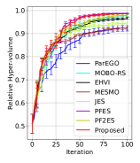
(a) $(d,L)=(2,2)$

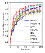
(b) $(d,L)=(2,3)$

(c) $(d,L)=(2,4)$

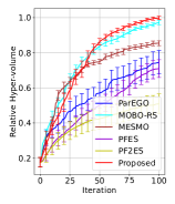
(d) $(d,L)=(2,5)$

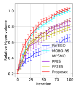
(e) $(d,L)=(2,6)$

(f) $(d,L)=(3,2)$

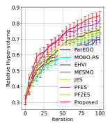
(g) $(d,L)=(3,3)$

(h) $(d,L)=(3,4)$

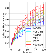
(i) $(d,L)=(3,5)$

(j) $(d,L)=(3,6)$

Figure 3: Performance comparison in GP-derived synthetic functions (average and standard deviation of $10$ runs).

PFEV is a general framework so that we can drive extensions for the following four scenarios:

Parallel querying:

In the parallel querying, we consider querying multiple points at one iteration, which is an important practical setting. Suppose that we consider $Q>1$ points selection. Let ${\cal X}_{q}\coloneqq\{\boldsymbol{x}^{(1)},\ldots,\boldsymbol{x}^{(q)}\}$ and ${\cal H}_{q}=\{\boldsymbol{f}_{\boldsymbol{x}^{(1)}},\ldots,\boldsymbol{f}_{\boldsymbol{x}^{(q)}}\}$ for $q\leq Q$. MI for all $Q$ points $\mathrm{MI}({\cal H}_{Q};{\cal F}^{*})$ represents the benefit of selecting ${\cal X}_{q}$, but this results in a $Q\times d$ dimensional optimization problem, which can be unstable. Instead, we follow an approach in (Takeno et al.,, 2022), which is a greedy selection based on conditional mutual information (CMI). When we select the $q+1$-th $\boldsymbol{x}$ after determining $\boldsymbol{x}^{(1)},\ldots,\boldsymbol{x}^{(q)}$, MI can be decomposed into

$$\mathrm{MI}({\cal H}_{q}\cup\boldsymbol{f}_{\boldsymbol{x}};{\cal F}^{*})\!=\!\mathrm{MI}({\cal H}_{q};{\cal F}^{*})\!+\!\mathrm{CMI}(\boldsymbol{f}_{\boldsymbol{x}};{\cal F}^{*}\mid{\cal H}_{q}),$$

where $\mathrm{CMI}(\boldsymbol{f}_{\boldsymbol{x}};{\cal F}^{*}\mid{\cal H}_{q})=\mathbb{E}_{{\cal H}_{q}}[\mathrm{MI}(\boldsymbol{f}_{\boldsymbol{x}};{\cal F}^{*}\mid{\cal H}_{q})]$ is the MI conditioned on ${\cal H}_{q}$. Since the first term does not depends on $\boldsymbol{x}$, we only need to optimize $\mathrm{CMI}$ to select $\boldsymbol{x}$. The calculation of $\mathrm{CMI}$ can be performed by adding sampled ${\cal H}_{q}$ into the training dataset of the GPs, after which evaluation of the lower bound is almost same as the single querying. See Appendix E for detail.

Decoupled setting:

In the decoupled setting, we can observe only one selected objective function instead of querying all $L$ objective functions simultaneously (Hernandez-Lobato et al.,, 2016). In PFEV, the criterion for the decoupled setting can be defined as $\mathrm{MI}(f^{l}_{\boldsymbol{x}};{\cal F}^{*})$, which is the information gain from only one objective function $f^{l}_{\boldsymbol{x}}$. The lower bound of $\mathrm{MI}(f^{l}_{\boldsymbol{x}};{\cal F}^{*})$ can be derived by the same approach shown in Section 3. In this case, we need to approximate $p(f^{l}_{\boldsymbol{x}}\mid{\cal F}^{*})$ instead of $p(\boldsymbol{f}_{\boldsymbol{x}}\mid{\cal F}^{*})$, for which we can use the marginal distribution of $q_{\lambda}(\boldsymbol{f}_{\boldsymbol{x}}\mid{\cal F}^{*})$. See Appendix F for detail.

Joint entropy search:

For PFEV, not only the information gain of the Pareto-frontier ${\cal F}^{*}$ but also the corresponding input $\boldsymbol{x}$ can be considered as $\mathrm{MI}(\boldsymbol{f}_{\boldsymbol{x}};{\cal X}^{*},{\cal F}^{*})$, where ${\cal X}^{*}=\{\boldsymbol{x}\mid\boldsymbol{f}_{\boldsymbol{x}}\in{\cal F}^{*}\}$. This can be seen as a JES extension of PFEV. When we derive the lower bound for $\mathrm{MI}(\boldsymbol{f}_{\boldsymbol{x}};{\cal X}^{*},{\cal F}^{*})$ by the same approach as Section 3, a variational approximation for $p(\boldsymbol{f}\mid{\cal X}^{*},{\cal F}^{*})$ is required. A basic idea of JES (Tu et al.,, 2022) is to simply add $({\cal X}^{*},{\cal F}^{*})$ into the training data of the GPs. In the case of PFEV, we can define the variational distribution $q(\boldsymbol{f}\mid{\cal X}^{*},{\cal F}^{*})$ by using the same mixture as (3). The only difference is that $({\cal X}^{*},{\cal F}^{*})$ is added to the training data of the GPs. Since we have not observed particular performance improvement by this additional conditioning, we employ $\mathrm{MI}(\boldsymbol{f}_{\boldsymbol{x}};{\cal F}^{*})$ as the default setting of PFEV. See Appendix G for detail.

Noisy observations:

It is also possible to derive the information gain obtained from noisy observation $\mathrm{MI}(\boldsymbol{y}_{\boldsymbol{x}};{\cal F}^{*})$, where $\boldsymbol{y}_{\boldsymbol{x}}=\boldsymbol{f}_{\boldsymbol{x}}+\boldsymbol{\varepsilon}$ with $\boldsymbol{\varepsilon}\sim{\cal N}(\boldsymbol{0},\sigma_{\rm noise}^{2}\boldsymbol{I})$, though we mainly consider $\mathrm{MI}(\boldsymbol{f}_{\boldsymbol{x}};{\cal F}^{*})$ for brevity. In this case, instead of $p(\boldsymbol{f}_{\boldsymbol{x}}\mid{\cal F}^{*})$, we need to consider $p(\boldsymbol{y}_{\boldsymbol{x}}\mid{\cal F}^{*})$. Through the relation $p(\boldsymbol{y}_{\boldsymbol{x}}\mid{\cal F}^{*})=\int p(\boldsymbol{y}_{\boldsymbol{x}}\mid\boldsymbol{f}_{\boldsymbol{x}})p(\boldsymbol{f}_{\boldsymbol{x}}\mid{\cal F}^{*})\mathrm{d}\boldsymbol{f}_{\boldsymbol{x}}$, we can derive the lower bound based on the same approximation of $p(\boldsymbol{f}_{\boldsymbol{x}}\mid{\cal F}^{*})$ by using $q_{\lambda}$. See Appendix H for detail.

6 Experiments

We empirically verify the performance of PFEV by comparing with ParEGO (Knowles,, 2006), EHVI (Emmerich,, 2005), MOBO-RS (Paria et al.,, 2020), MESMO (Belakaria et al.,, 2019), PFES (Suzuki et al.,, 2020), $\{\text{PF}\}^{2}\text{ES}$ (Qing et al.,, 2022), and JES (Tu et al.,, 2022). We used GP-based synthetic functions and benchmark functions.

Each evaluation run $10$ times. As a performance metric, RHV (relative hyper-volume) was used. RHV is defined as the hyper-volume of the observed Pareto-frontier divided by the volume of the reference Pareto-frontier. The reference Pareto-frontier was obtained by $10,000$ iterations of NSGA-II. All the methods used GPs for $f^{l}_{\boldsymbol{x}}$ with a kernel function $k(\boldsymbol{x},\boldsymbol{x}^{\prime})=\exp(-\|\boldsymbol{x}-\boldsymbol{x}^{\prime}\|_{2}^{2}/(2\ell^{2}_{\rm RBF}))$, where $\ell_{\rm RBF}\in\mathbb{R}$ is a hyper-parameter. The marginal likelihood maximization was performed at every iteration to optimize $\ell_{\rm RBF}$. The number of samplings of the optimal value or the Pareto-frontier in MESMO, PFES, $\{$PF$\}^{2}$ES, and PFEV was $10$, each of which was performed by NSGA-II ($1,000$ generations and population size $50$). We used DIRECT algorithm (Jones et al.,, 1993) for the acquisition function maximization. We selected $5$ random $\boldsymbol{x}$ as the initial points. EHVI and JES were performed up to $L=4$. Other settings are described in Appendix J.

6.1 Synthetic Functions Generated by GPs

Here, we consider synthetic functions from GPs as true objective functions, i.e., $f^{\ell}\sim\mathcal{GP}(0,k)$, in which $\ell_{\rm RBF}=0.1$ was used in the kernel $k$. Since we require objective functions in a continuous domain, we used the RFM-based approximation (the number of RFM basis is $D=1000$). The input dimension is $d\in\{2,3\}$, and the domain ${\cal X}$ is $[0,1]^{d}$. The output dimensions are $L\in\{2,3,4,5,6\}$.

(a) $L=2$

(b) $L=3$

(c) $L=4$

(d) $L=5$

(e) $L=6$

Figure 4: Boxplots of RHV at $100$-th iteration.

Figure 3 shows the results. In all (a)-(j), PFEV shows superior or comparable performance to existing methods. In this experiment, we empirically see that the performance of PFEV is often similar to PFES and $\{\text{PF}\}^{2}\text{ES}$ for $L=2$, and differences become clearer for $L\geq 3$. This can also be confirmed by Fig. 4, which shows boxplots of RHV at the $100$-th iteration in all trials of Fig. 3. This result is consistent with our conjecture about the difference of two types of PFTN described in Section 3.2. In Appendix K.1, additional results on different $\ell_{\rm RBF}$ and $d=4$ are shown, in which similar tendency was confirmed.

6.2 Benchmark Functions

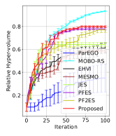
(a) Fonseca Fleming

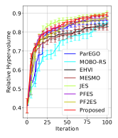
(b) Kursawe

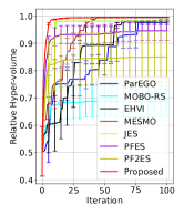
(c) Viennet

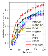
(d) FES3

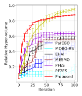
(e) Fonseca$+$Viennet

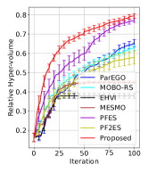
(f) FES3$+$Kursawe

Figure 5: Performance comparison in benchmark functions (average and standard deviation of $10$ runs).

We used benchmark problems called Fonseca Fleming $(d,L)=(2,2)$, Kursawe $(d,L)=(3,2)$, Viennet $(d,L)=(2,3)$ and FES3 $(d,L)=(3,4)$ problems (for detail, see Appendix J). Further, we combine multiple problems having the same input dimensions, i.e., we created Fonseca$+$Viennet $(d,L)=(2,5)$ and FES3$+$Kursawe $(d,L)=(3,6)$. Since the input domain is shared (which is scaled to $[0,1]^{d}$ beforehand), only the output dimension is increased compared with the original problems. The results are shown in Fig. 5. Overall, the performance of proposed PFEV is high among compared methods. Here again, we see that in problems with the output dimension $\geq 3$, PFEV tends to show its advantage. Additional results on benchmark functions are also shown in Appendix K.2.

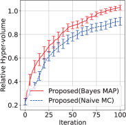
(a) $(d,L)=(2,6)$

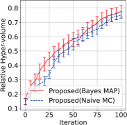
(b) $(d,L)=(3,6)$

Figure 6: Comparison between two MC estimators (6) and (8) of PFEV using GP-derived synthetic functions.

6.3 Comparison of PFEV with Different MC Estimators

By using GP-derived synthetic functions, two estimators of PFEV (6) and (8) are compared. The same settings as Section 6.1 were used. The results of $(d,L)=(2,6)$ and $(d,L)=(3,6)$ are shown in Fig. 6. We see that the MAP-based approximation (8) improves the performance compared with (6). We confirmed similar results on other GP-derived functions, which is summarized in Fig. 17 in Appendix K.1.

7 Conclusions

We proposed a multi-objective Bayesian optimization acquisition function that is based on the variational lower bound maximization. By combining two normal distributions, defined by under and over truncation of Pareto-frontier, we introduced a variational distribution as mixture of these two distributions based on which a lower bound of mutual information can be constructed. Performance superiority was shown by GP generated functions and benchmark functions. A current limitation includes theoretical guarantee of the MI approximation and convergence, which is important open problems for information theoretic BO.

Appendix A Proof of Remark 3.2

The lower bound of (5) is derived by using the case of $\lambda=1$:

$$\max_{\lambda\in(0,1]}L(\boldsymbol{x},\lambda) \geq L(\boldsymbol{x},1)=\mathbb{E}_{{\cal F}^{*},\boldsymbol{f}_{\boldsymbol{x}}}\left[\log\left(\frac{q_{U}(\boldsymbol{f}_{\boldsymbol{x}}\mid{\cal F}_{S}^{*})}{p(\boldsymbol{f}_{\boldsymbol{x}})}\right)\right]$$

$$=-\mathbb{E}_{{\cal F}^{*}}\left[\int_{{\cal A}_{U}^{{\cal F}_{S}^{*}}}p(\boldsymbol{f}_{\boldsymbol{x}}\mid{\cal F}^{*})\log Z_{U}^{{\cal F}^{*}_{S}}(\boldsymbol{x})\mathrm{d}\boldsymbol{f}_{\boldsymbol{x}}\right]$$

$$=-\mathbb{E}_{{\cal F}^{*}}\left[\log Z_{U}^{{\cal F}^{*}_{S}}(\boldsymbol{x})\right]$$

$$=-\mathbb{E}_{{\cal F}^{*}}\left[\log(1-p(\boldsymbol{f}_{\boldsymbol{x}}\notin{\cal A}_{U}^{{\cal F}_{S}^{*}}))\right]$$

$$\geq\mathbb{E}_{{\cal F}^{*}}\left[p(\boldsymbol{f}_{\boldsymbol{x}}\notin{\cal A}_{U}^{{\cal F}_{S}^{*}})\right]>0$$

Appendix B Computations of $Z_{O}^{\tilde{{\cal F}}^{*}_{S}}$ and $Z_{U}^{\tilde{{\cal F}}^{*}_{S}}$

First, we consider the normalization constant of PFTN-O $Z_{O}^{\tilde{{\cal F}}^{*}_{S}}=p(\boldsymbol{f}_{\boldsymbol{x}}\in{\cal A}_{O}^{{\cal F}^{*}_{S}})$. We decompose ${\cal A}_{O}^{\tilde{{\cal F}}^{*}_{S}}$ into disjoint hyper-rectangles, denoted as ${\cal A}_{O}^{\tilde{{\cal F}}^{*}_{S}}={\cal C}_{1}\cup{\cal C}_{2}\cup\ldots\cup{\cal C}_{C}$, where ${\cal C}_{i}$ is a hyper-rectangle and $C$ is the number of hyper-rectangles. Algorithms decomposing a dominated region have been studied in the context of the Pareto hyper-volume computation. We use Quick Hyper-volume (QHV) (Russo and Francisco,, 2014), used also in PFES. Each hyper-rectangle ${\cal C}_{i}$ is written as

$${\cal C}_{i}=\left(\ell_{i}^{1},u_{i}^{1}\right]\times\left(\ell_{i}^{2},u_{i}^{2}\right]\times\ldots\times\left(\ell_{i}^{L},u_{i}^{L}\right],$$

where $\ell_{i}^{l}$ and $u_{i}^{l}$ are the smallest and largest values in the $l$-th dimension of the $i$-th hyper-rectangle. From the independence of the objective functions, $Z_{O}^{\tilde{{\cal F}}^{*}_{S}}$ can be easily computed by

$$Z_{O}^{\tilde{{\cal F}}^{*}_{S}} =\sum_{i=1}^{C}\int_{{\cal C}_{i}}p(\boldsymbol{f}_{\boldsymbol{x}})\mathrm{d}\boldsymbol{f}_{\boldsymbol{x}}$$

$$=\sum_{i=1}^{C}\prod_{l=1}^{L}\int_{\ell_{i}^{l}}^{u_{i}^{l}}p(f_{\boldsymbol{x}}^{l})\mathrm{d}f_{\boldsymbol{x}}^{l}$$

$$=\sum_{i=1}^{C}\prod_{l=1}^{L}\left(\Phi(\bar{\alpha}_{i,l})-\Phi(\underline{\alpha}_{i,l})\right),$$ (9)

where $\underline{\alpha}_{i,l}=(\ell_{i}^{l}-\mu_{l}(\boldsymbol{x}))/\sigma_{l}(\boldsymbol{x})$ and $\bar{\alpha}_{i,l}=(u_{i}^{l}-\mu_{l}(\boldsymbol{x}))/\sigma_{l}(\boldsymbol{x})$, and $\Phi$ is the cumulative distribution function of the standard normal distribution.

Next, we consider $Z_{U}^{\tilde{{\cal F}}^{*}_{S}}$ that can be re-written as

$$Z_{U}^{\tilde{{\cal F}}^{*}_{S}} =p\left(\boldsymbol{f}_{\boldsymbol{x}}\in{\cal A}_{U}^{\tilde{{\cal F}}^{*}_{S}}\right)$$

$$=1-p\left(\boldsymbol{f}_{\boldsymbol{x}}\notin{\cal A}_{U}^{\tilde{{\cal F}}^{*}_{S}}\right)$$

$$=1-p\left(-\boldsymbol{f}_{\boldsymbol{x}}\preceq\{-\boldsymbol{f}\mid\boldsymbol{f}\in\tilde{{\cal F}}^{*}_{S}\}\right).$$

In the last equation, the region $\boldsymbol{f}_{\boldsymbol{x}}\notin{\cal A}_{U}^{\tilde{{\cal F}}^{*}_{S}}$ is re-written by flipping the sign of $\tilde{{\cal F}}^{*}_{S}$ in such a way that the region is written as a “dominated region”. This enable us to use QHV, which decomposes a “dominated region” into hyper-rectangles, for the computation of $p(-\boldsymbol{f}_{\boldsymbol{x}}\preceq\{-\boldsymbol{f}\mid\boldsymbol{f}\in\tilde{{\cal F}}^{*}_{S}\})$ based on almost the same way as (9).

Appendix C Concavity of Acquisition Function about $\lambda$

To simplify the notation, we unify (8) and (6) as

$$\widehat{L}(\boldsymbol{x},\boldsymbol{\lambda}) =\frac{1}{K}\sum_{(\tilde{{\cal F}}^{*}_{S},\tilde{\boldsymbol{f}})\in F}\log\left(\frac{\lambda}{Z_{U}}+\frac{1-\lambda}{Z_{O}}\right)\xi(\tilde{\boldsymbol{f}_{\boldsymbol{x}}})$$

$$\qquad+\log\left(\frac{\lambda}{Z_{U}}\right)(1-\xi(\tilde{\boldsymbol{f}_{\boldsymbol{x}}})),$$

where $Z_{U}=Z_{U}^{\tilde{{\cal F}}^{*}_{S}}(\boldsymbol{x})$, $Z_{O}=Z_{O}^{\tilde{{\cal F}}^{*}_{S}}(\boldsymbol{x})$, and $\xi(\tilde{\boldsymbol{f}_{\boldsymbol{x}}})=\theta_{\mathrm{MAP}}(\tilde{\boldsymbol{f}_{\boldsymbol{x}}})$ when (8), and $\xi(\tilde{\boldsymbol{f}_{\boldsymbol{x}}})=\mathbb{I}(\tilde{\boldsymbol{f}_{\boldsymbol{x}}}\in{\cal A}_{O}^{\tilde{{\cal F}}^{*}_{S}})$ when (6). The second derivative is

$${\frac{\partial^{2}\widehat{L}(\boldsymbol{x},\lambda)}{\partial\lambda^{2}}} =\frac{1}{K}\sum_{(\tilde{{\cal F}}^{*}_{S},\tilde{\boldsymbol{f}})\in F}-\left(\frac{Z_{O}-Z_{U}}{\lambda(Z_{O}-Z_{U})+Z_{U}}\right)^{2}\xi(\tilde{\boldsymbol{f}_{\boldsymbol{x}}})$$

$$\qquad-\frac{1}{\lambda^{2}}(1-\xi(\tilde{\boldsymbol{f}_{\boldsymbol{x}}}))\leq 0.$$

Thus, we see concavity.

Appendix D Combining Prior Knowledge in MC Estimator

D.1 Derivation of MAP

We use the beta distribution for the prior $\theta\sim\mathrm{beta}(a,b)$. The density function is

$$p(\theta)=\frac{\theta^{a-1}(1-\theta)^{b-1}}{B(a,b)}.$$

Using the approximation $\theta\approx\hat{p}$, we set $a-1=r\hat{p}$ and $b-1=r(1-\hat{p})$, where $r\geq 0$ is a parameter. This sets the mode of $p(\theta)$ as $\hat{p}$. As shown in Fig. 7, a larger $r$ has a stronger peak at $\hat{p}$. When $r=0$, $p(\theta)$ becomes uniform in $[0,1]$.

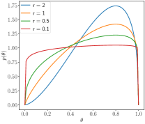
Figure 7: Density functions of the beta distribution when $\hat{p}=0.8$. For all $r$, the mode is $0.8$.

The posterior of the beta distribution with the Bernoulli distribution likelihood is $\mathrm{beta}(a+m,a+\ell)$, where $m$ is the number of ‘success’ and $\ell$ is the number of ‘fail’ in Bernoulli trials. We can interpret that $\mathbb{I}(\boldsymbol{f}_{\boldsymbol{x}}\in{\cal A}_{O}^{{\cal F}^{*}_{S}})$ is a sample from the Bernoulli distribution with the probability $p(\boldsymbol{f}_{\boldsymbol{x}}\in{\cal A}_{O}^{\tilde{{\cal F}}^{*}_{S}}\mid{\cal F}^{*})$. Therefore, we set $m=\mathbb{I}(\boldsymbol{f}_{\boldsymbol{x}}\in{\cal A}_{O}^{{\cal F}^{*}_{S}})$ and $\ell=1-\mathbb{I}(\boldsymbol{f}_{\boldsymbol{x}}\in{\cal A}_{O}^{{\cal F}^{*}_{S}})$, from which the mode of the posterior $\mathrm{beta}(a+m,a+\ell)$ can be derived as

$$\theta_{\mathrm{MAP}} =\frac{a-1+m}{a-1+m+b-1+\ell}$$

$$=\frac{r\hat{p}+\mathbb{I}(\boldsymbol{f}_{\boldsymbol{x}}\in{\cal A}_{O}^{{\cal F}^{*}_{S}})}{r\hat{p}+\mathbb{I}(\boldsymbol{f}_{\boldsymbol{x}}\in{\cal A}_{O}^{{\cal F}^{*}_{S}})+r(1-\hat{p})+(1-\mathbb{I}(\boldsymbol{f}_{\boldsymbol{x}}\in{\cal A}_{O}^{{\cal F}^{*}_{S}}))}$$

$$=\frac{r\hat{p}+\mathbb{I}(\boldsymbol{f}_{\boldsymbol{x}}\in{\cal A}_{O}^{{\cal F}^{*}_{S}})}{r+1}.$$

In the main text, we employ $r=1$.

The lower bound estimation by MAP (8) can have an estimation bias caused by the approximation $\hat{p}$, though it is almost negligible when $K$ is a typical setting (such as $K=10$). This bias occurs because, we only have one $\tilde{\boldsymbol{f}}_{\boldsymbol{x}}$ for each corresponding $\tilde{{\cal F}}^{*}_{S}$. Therefore, in each $\theta_{\mathrm{MAP}}$, the effect of the prior remains even when $K$ is large. We can easily avoid this bias by setting $r$ so that it decreases $r\rightarrow 0$ when $K$ increases, by which the estimator (8) converges to the usual MC estimator (6). In Appendix D.3, we show that, in practice, the MAP based approach has an advantage for small $K$ setting.

D.2 Analyzing Variance

We re-write the estimator of the lower bound (8) as

$$\frac{1}{K}\sum_{(\tilde{{\cal F}}^{*}_{S},\tilde{\boldsymbol{f}})\in F}a(\tilde{{\cal F}}^{*}_{S})\xi(\tilde{\boldsymbol{f}_{\boldsymbol{x}}})+b(\tilde{{\cal F}}^{*}_{S}).$$

where $a(\tilde{{\cal F}}^{*}_{S})=\log\left(\frac{\lambda}{Z_{U}^{\tilde{{\cal F}}^{*}_{S}}(\boldsymbol{x})}+\frac{1-\lambda}{Z_{O}^{\tilde{{\cal F}}^{*}_{S}}(\boldsymbol{x})}\right)-\log\left(\frac{\lambda}{Z_{U}^{\tilde{{\cal F}}^{*}_{S}}(\boldsymbol{x})}\right)$, $b(\tilde{{\cal F}}^{*}_{S})=\log\left(\frac{\lambda}{Z_{U}^{\tilde{{\cal F}}^{*}_{S}}(\boldsymbol{x})}\right)$, and $\xi(\tilde{\boldsymbol{f}_{\boldsymbol{x}}})\in[0,1]$ is $\theta_{\mathrm{MAP}}(\tilde{\boldsymbol{f}_{\boldsymbol{x}}})$ when (8) and is $\mathbb{I}(\tilde{\boldsymbol{f}_{\boldsymbol{x}}}\in{\cal A}_{O}^{\tilde{{\cal F}}^{*}_{S}})$ when (6). By using independence of the MC samples and law of total variance, the variance of this estimator is decomposed as follows:

$$\mathbb{V}_{\tilde{{\cal F}}^{*},\tilde{\boldsymbol{f}}}\left[\frac{1}{K}\sum_{(\tilde{{\cal F}}^{*}_{S},\tilde{\boldsymbol{f}})\in F}a(\tilde{{\cal F}}^{*}_{S})\xi(\tilde{\boldsymbol{f}_{\boldsymbol{x}}})+b(\tilde{{\cal F}}^{*}_{S})\right]$$

$$=\frac{1}{K}\mathbb{E}_{\tilde{{\cal F}}^{*}}\mathbb{V}_{\tilde{\boldsymbol{f}}\mid\tilde{{\cal F}}^{*}}\left[a(\tilde{{\cal F}}^{*}_{S})\xi(\tilde{\boldsymbol{f}_{\boldsymbol{x}}})+b(\tilde{{\cal F}}^{*}_{S})\right]$$

$$\qquad+\frac{1}{K}\mathbb{V}_{\tilde{{\cal F}}^{*}}\mathbb{E}_{\tilde{\boldsymbol{f}}\mid\tilde{{\cal F}}^{*}}\left[a(\tilde{{\cal F}}^{*}_{S})\xi(\tilde{\boldsymbol{f}_{\boldsymbol{x}}})+b(\tilde{{\cal F}}^{*}_{S})\right]$$

$$=\frac{1}{K}\biggl{\{}\mathbb{E}_{\tilde{{\cal F}}^{*}}\left[a(\tilde{{\cal F}}^{*}_{S})^{2}\mathbb{V}_{\tilde{\boldsymbol{f}}\mid\tilde{{\cal F}}^{*}}\left[\xi(\tilde{\boldsymbol{f}_{\boldsymbol{x}}})\right]\right]+\mathbb{E}_{\tilde{{\cal F}}^{*}}\left[b(\tilde{{\cal F}}^{*}_{S})\right]$$

$$\qquad+\mathbb{V}_{\tilde{{\cal F}}^{*}}\left[a(\tilde{{\cal F}}^{*}_{S})\mathbb{E}_{\tilde{\boldsymbol{f}}\mid\tilde{{\cal F}}^{*}}\left[\xi(\tilde{\boldsymbol{f}_{\boldsymbol{x}}})\right]+b(\tilde{{\cal F}}^{*}_{S})\right]\biggr{\}}$$ (10)

In the first term of (10), only $\mathbb{V}_{\tilde{\boldsymbol{f}}\mid\tilde{{\cal F}}^{*}}\left[\xi(\tilde{\boldsymbol{f}_{\boldsymbol{x}}})\right]$ changes depending on $\xi$. From

$$\mathbb{V}_{\tilde{\boldsymbol{f}}\mid\tilde{{\cal F}}^{*}}\left[\theta_{\mathrm{MAP}}(\tilde{\boldsymbol{f}_{\boldsymbol{x}}})\right]=\mathbb{V}_{\tilde{\boldsymbol{f}}\mid\tilde{{\cal F}}^{*}}\left[\mathbb{I}(\tilde{\boldsymbol{f}_{\boldsymbol{x}}}\in{\cal A}_{O}^{\tilde{{\cal F}}^{*}_{S}})\right]/4,$$

we see that MAP makes the variance of the first term $1/4$. The second term in (10) does not change depending on $\xi$. In the case of the MAP estimate, the third term in (10) is

$$\mathbb{V}_{\tilde{{\cal F}}^{*}}\left[a(\tilde{{\cal F}}^{*}_{S})\mathbb{E}_{\tilde{\boldsymbol{f}}\mid\tilde{{\cal F}}^{*}}\left[\xi(\tilde{\boldsymbol{f}_{\boldsymbol{x}}})\right]+b(\tilde{{\cal F}}^{*}_{S})\right]$$

$$=\mathbb{V}_{\tilde{{\cal F}}^{*}}\left[a(\tilde{{\cal F}}^{*}_{S})\mathbb{E}_{\tilde{\boldsymbol{f}}\mid\tilde{{\cal F}}^{*}}\left[\frac{\hat{p}+\mathbb{I}(\tilde{\boldsymbol{f}_{\boldsymbol{x}}}\in{\cal A}_{O}^{\tilde{{\cal F}}^{*}_{S}})}{2}\right]+b(\tilde{{\cal F}}^{*}_{S})\right]$$

$$=\mathbb{V}_{\tilde{{\cal F}}^{*}}\left[a(\tilde{{\cal F}}^{*}_{S})\frac{\hat{p}+p(\tilde{\boldsymbol{f}_{\boldsymbol{x}}}\in{\cal A}_{O}^{\tilde{{\cal F}}^{*}_{S}}\mid\tilde{{\cal F}}^{*})}{2}+b(\tilde{{\cal F}}^{*}_{S})\right].$$

If $\hat{p}\approx p(\tilde{\boldsymbol{f}_{\boldsymbol{x}}}\in{\cal A}_{O}^{\tilde{{\cal F}}^{*}_{S}}\mid\tilde{{\cal F}}^{*})$, this should be similar to $\mathbb{V}_{\tilde{{\cal F}}^{*}}\left[a(\tilde{{\cal F}}^{*}_{S})p(\tilde{\boldsymbol{f}_{\boldsymbol{x}}}\in{\cal A}_{O}^{\tilde{{\cal F}}^{*}_{S}}\mid\tilde{{\cal F}}^{*})+b(\tilde{{\cal F}}^{*}_{S})\right]$, which is the variance in the case of $\xi(\tilde{\boldsymbol{f}_{\boldsymbol{x}}})=\mathbb{I}(\tilde{\boldsymbol{f}_{\boldsymbol{x}}}\in{\cal A}_{O}^{\tilde{{\cal F}}^{*}_{S}})$. Therefore, under the assumption of $\hat{p}\approx p(\tilde{\boldsymbol{f}_{\boldsymbol{x}}}\in{\cal A}_{O}^{\tilde{{\cal F}}^{*}_{S}}\mid\tilde{{\cal F}}^{*})$ the variance reduction is expected because of the variance reduction in the first term of (10).

D.3 Empirical Verification of MC Estimator of Lower Bound

Using a two objective problem generated by GPs ($d=1$), we examine the accuracy of the MC estimator compared with the true lower bound. Hereafter, Naïve MC indicates the calculation by (6), and MC with Bayes MAP indicates the calculation by (8). We calculate the lower bound at $100$ grid points in $x\in[0,1]$ with random $5$ training points. Regarding the result by Naïve MC with $K=10^{5}$ samples as a pseudo ground-truth, compared with which we evaluate the estimation error. In addition to the fixed $r$ setting, we here examine the setting $r=\sqrt{10/K}$, by which $r$ reduces with $O(1/\sqrt{K})$ (same as the general convergence rate of the MC estimator) and $r=1$ when $K=10$ in this setting.

Figure 8 shows the results by mean squared error (MSE). MC with Bayes MAP shows $r=1$ and $r=\sqrt{10/K}$, for which they have the same result when $K=10$. When the sample size $K$ is small, MC with Bayes MAP has smaller errors for both the $r$ settings compared with Naïve MC. With the increase of $K$, all methods decrease MSE, but in the right log scale plot, the decrease of MC with Bayes MAP ($r=1$) stagnates at around $K=10^{2}$–$10^{3}$. On the other hand, MC with Bayes MAP ($r=\sqrt{10/K}$) continues to decrease MSE because it can diminish the effect of the approximation in the prior.

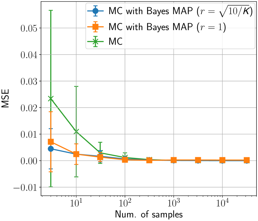
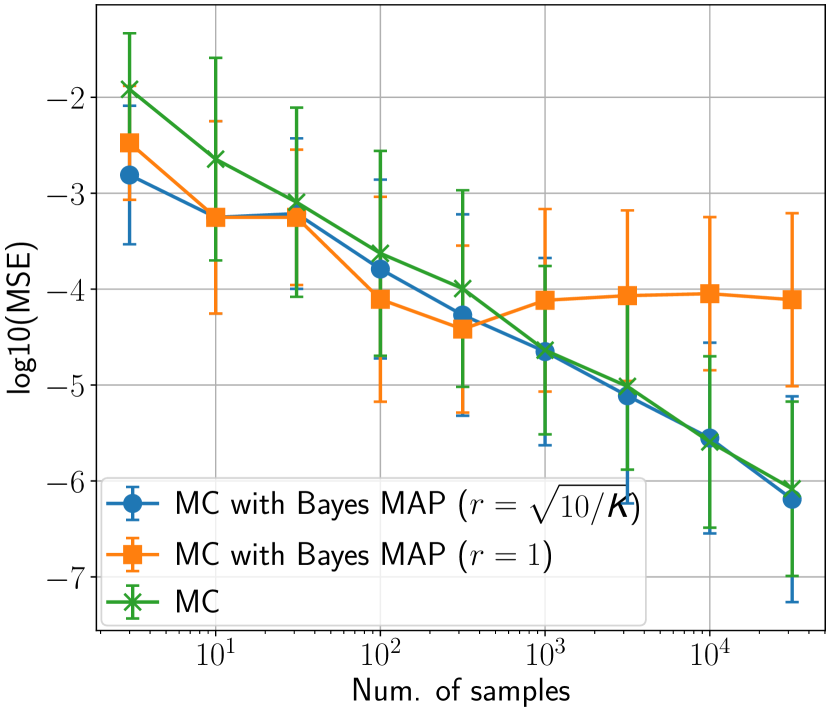
Figure 8: MSE compared with the pseudo ground truth, created by Naïve MC with $K=10^{5}$. The plot is the original scale, and the right plot is the $\log_{10}$ scale.

Appendix E Parallel Querying

We here consider parallel querying in which $Q$ queries should be selected every iteration. Let ${\cal X}_{q}\coloneqq\{\boldsymbol{x}^{(1)},\ldots,\boldsymbol{x}^{(q)}\}$ and ${\cal H}_{q}=\{\boldsymbol{f}_{\boldsymbol{x}^{(1)}},\ldots,\boldsymbol{f}_{\boldsymbol{x}^{(q)}}\}$ for $q\leq Q$. Then, $\mathrm{MI}({\cal H}_{Q};{\cal F}^{*})$ can be a selection criterion for determining $Q$ points simultaneously. However, this leads to $Q\times d$ dimensional optimization. Instead, we employ a greedy strategy shown by (Takeno et al.,, 2022), in which the MI approximation can be reduced to a similar computation to the case of single querying.

Assume that we already select $q<Q$ points ${\cal X}_{q}$, for which observations are not obtained yet, and consider determining the $q+1$-th point $\boldsymbol{x}$. In this case, $\mathrm{MI}({\cal H}_{q}\cup\boldsymbol{f}_{\boldsymbol{x}};{\cal F}^{*})$ should be maximized with respect to the additional $\boldsymbol{x}$. We see

$$\mathrm{MI}({\cal H}_{q}\cup\boldsymbol{f}_{\boldsymbol{x}};{\cal F}^{*})=\mathrm{MI}({\cal H}_{q};{\cal F}^{*})+\mathrm{CMI}(\boldsymbol{f}_{\boldsymbol{x}};{\cal F}^{*}\mid{\cal H}_{q}),$$

where $\mathrm{CMI}(\boldsymbol{f}_{\boldsymbol{x}};{\cal F}^{*}\mid{\cal H}_{q})=\mathbb{E}_{{\cal H}_{q}}\left[\mathrm{MI}(\boldsymbol{f}_{\boldsymbol{x}};{\cal F}^{*}\mid{\cal H}_{q})\right]$ is the MI conditioned on ${\cal H}_{q}$. Since the first term does not depend on $\boldsymbol{x}$, we only need to consider the second term $\mathrm{CMI}(\boldsymbol{f}_{\boldsymbol{x}};{\cal F}^{*}\mid{\cal H}_{q})$.

The lower bound of $\mathrm{MI}(\boldsymbol{f}_{\boldsymbol{x}};{\cal F}^{*}\mid{\cal H}_{q})$ is derived by the same way as the lower bound of $\mathrm{MI}(\boldsymbol{f}_{\boldsymbol{x}};{\cal F}^{*})$, i.e., (4). The only difference is that the GPs have additional training data consisting of ${\cal X}_{q}$ and ${\cal H}_{q}$. Let $\zeta_{\lambda,q}^{{\cal F}^{*}_{S}}(\boldsymbol{x})$ and $\eta_{\lambda,q}^{{\cal F}^{*}_{S}}(\boldsymbol{x})$ be $\zeta_{\lambda}^{{\cal F}^{*}_{S}}(\boldsymbol{x})$ and $\eta_{\lambda}^{{\cal F}^{*}_{S}}(\boldsymbol{x})$ in which the GPs with additional $q$ observations are used to calculate $Z_{U}^{{\cal F}_{S}^{*}}(\boldsymbol{x})$ and $Z_{O}^{{\cal F}_{S}^{*}}(\boldsymbol{x})$ as follows:

$$\zeta_{\lambda,q}^{{\cal F}^{*}_{S}}(\boldsymbol{x}) =\frac{\lambda}{Z_{U}^{{\cal F}^{*}_{S}}(\boldsymbol{x}\mid{\cal H}_{q})}+\frac{1-\lambda}{Z_{O}^{{\cal F}^{*}_{S}}(\boldsymbol{x}\mid{\cal H}_{q})},$$

$$\eta_{\lambda,q}^{{\cal F}^{*}_{S}}(\boldsymbol{x}) =\frac{\lambda}{Z_{U}^{{\cal F}^{*}_{S}}(\boldsymbol{x}\mid{\cal H}_{q})},$$

where $Z_{U}^{{\cal F}^{*}_{S}}(\boldsymbol{x}\mid{\cal H}_{q})\coloneqq p(\boldsymbol{f}_{\boldsymbol{x}}\in{\cal A}_{U}^{{\cal F}^{*}_{S}}\mid{\cal H}_{q})$ and $Z_{O}^{{\cal F}^{*}_{S}}(\boldsymbol{x}\mid{\cal H}_{q})\coloneqq p(\boldsymbol{f}_{\boldsymbol{x}}\in{\cal A}_{O}^{{\cal F}^{*}_{S}}\mid{\cal H}_{q})$. Then, we can write

$$\mathbb{E}_{{\cal H}_{q}}\left[\mathrm{MI}(\boldsymbol{f}_{\boldsymbol{x}};{\cal F}^{*}\mid{\cal H}_{q})\right]$$

$$\geq\mathbb{E}_{{\cal H}_{q}}\mathbb{E}_{{\cal F}^{*},\boldsymbol{f}_{\boldsymbol{x}}\mid{\cal H}_{q}}\biggl{[}\log\bigl{\{}\zeta_{\lambda,q}^{{\cal F}^{*}_{S}}(\boldsymbol{x})\mathbb{I}(\boldsymbol{f}_{\boldsymbol{x}}\in{\cal A}_{O}^{{\cal F}^{*}_{S}})$$

$$\qquad\qquad\qquad+\eta_{\lambda,q}^{{\cal F}^{*}_{S}}(\boldsymbol{x})\mathbb{I}(\boldsymbol{f}_{\boldsymbol{x}}\in{\cal A}_{U\setminus O}^{{\cal F}^{*}_{S}})\bigr{\}}\biggr{]}$$

$$=\mathbb{E}_{{\cal F}^{*},\boldsymbol{f}_{\boldsymbol{x}},{\cal H}_{q}}\biggl{[}\log\bigl{\{}\zeta_{\lambda,q}^{{\cal F}^{*}_{S}}(\boldsymbol{x})\mathbb{I}(\boldsymbol{f}_{\boldsymbol{x}}\in{\cal A}_{O}^{{\cal F}^{*}_{S}})$$

$$\qquad\qquad\qquad+\eta_{\lambda,q}^{{\cal F}^{*}_{S}}(\boldsymbol{x})\mathbb{I}(\boldsymbol{f}_{\boldsymbol{x}}\in{\cal A}_{U\setminus O}^{{\cal F}^{*}_{S}})\bigr{\}}\biggr{]}$$ (11)

Since the expectation $\mathbb{E}_{{\cal H}_{q}}\mathbb{E}_{{\cal F}^{*},\boldsymbol{f}_{\boldsymbol{x}}\mid{\cal H}_{q}}$ can be seen as the joint expectation $\mathbb{E}_{{\cal F}^{*},\boldsymbol{f}_{\boldsymbol{x}},{\cal H}_{q}}$, the MC approximation can be performed by using sample from the joint distribution of ${\cal F}^{*},\boldsymbol{f}_{\boldsymbol{x}}$ and ${\cal H}_{q}$. Let $F_{q}$ be a set of samples $(\tilde{{\cal F}}^{*}_{S},\tilde{\boldsymbol{f}}_{\boldsymbol{x}},\tilde{{\cal H}}_{q})$ from the joint distribution. Then, the MC approximation of the lower bound (11) is

$$\frac{1}{K}\sum_{(\tilde{{\cal F}}^{*}_{S},\tilde{\boldsymbol{f}}_{\boldsymbol{x}},\tilde{{\cal H}}_{q})\in F_{q}}\log\bigl{\{}\zeta_{\lambda,q}^{\tilde{{\cal F}}^{*}_{S}}(\boldsymbol{x})\mathbb{I}(\tilde{\boldsymbol{f}}_{\boldsymbol{x}}\in{\cal A}_{O}^{\tilde{{\cal F}}^{*}_{S}})$$

$$\qquad\qquad\qquad+\eta_{\lambda,q}^{\tilde{{\cal F}}^{*}_{S}}(\boldsymbol{x})\mathbb{I}(\tilde{\boldsymbol{f}_{\boldsymbol{x}}}\in{\cal A}_{U\setminus O}^{\tilde{{\cal F}}^{*}_{S}})\bigr{\}}$$

The sampling of $F_{q}$ can be performed by almost the same procedure as the single querying. First, we generate the “entire function $\tilde{\boldsymbol{f}}$” by using RFM. $\tilde{{\cal F}}^{*}_{S}$ is obtained by applying NSGA-II to $\tilde{\boldsymbol{f}}$. $\tilde{\boldsymbol{f}}_{\boldsymbol{x}}$ and $\tilde{{\cal H}}_{q}$ can be immediately obtained from RFM. Note that even when we perform next $q+2$-th point selection, we can reuse $\tilde{{\cal F}}^{*}_{S}$ and $\tilde{\boldsymbol{f}}$, from which $\tilde{{\cal H}}_{q+1}$ can also be immediately obtained.

The MAP based approximation can also be applied to the parallel setting. The lower bound (11) can be re-written as

$$\mathbb{E}_{{\cal F}^{*},{\cal H}_{q}}\mathbb{E}_{\boldsymbol{f}_{\boldsymbol{x}}\mid{\cal F}^{*},{\cal H}_{q}}\biggl{[}\mathbb{I}(\boldsymbol{f}_{\boldsymbol{x}}\in{\cal A}_{O}^{{\cal F}^{*}_{S}})\log\zeta_{\lambda,q}^{{\cal F}^{*}_{S}}(\boldsymbol{x})$$

$$\qquad\qquad\qquad+\mathbb{I}(\boldsymbol{f}_{\boldsymbol{x}}\in{\cal A}_{U\setminus O}^{{\cal F}^{*}_{S}})\log\eta_{\lambda,q}^{{\cal F}^{*}_{S}}(\boldsymbol{x})\biggr{]}$$

$$=\mathbb{E}_{{\cal F}^{*},{\cal H}_{q}}\biggl{[}p(\boldsymbol{f}_{\boldsymbol{x}}\in{\cal A}_{O}^{{\cal F}^{*}_{S}}\mid{\cal F}^{*},{\cal H}_{q})\log\zeta_{\lambda,q}^{{\cal F}^{*}_{S}}(\boldsymbol{x})$$

$$\qquad\qquad\qquad+p(\boldsymbol{f}_{\boldsymbol{x}}\in{\cal A}_{U\setminus O}^{{\cal F}^{*}_{S}}\mid{\cal F}^{*},{\cal H}_{q})\log\eta_{\lambda,q}^{{\cal F}^{*}_{S}}(\boldsymbol{x})\bigr{\}}\biggr{]}.$$

The prior approximation for $p(\boldsymbol{f}_{\boldsymbol{x}}\in{\cal A}_{O}^{{\cal F}^{*}_{S}}\mid{\cal F}^{*},{\cal H}_{q})$ becomes $p(\boldsymbol{f}_{\boldsymbol{x}}\in{\cal A}_{O}^{{\cal F}^{*}_{S}}\mid{\cal F}^{*},{\cal H}_{q})\approx Z_{O}^{{\cal F}^{*}_{S}}(\boldsymbol{x}\mid{\cal H}_{q})/Z_{U}^{{\cal F}^{*}_{S}}(\boldsymbol{x}\mid{\cal H}_{q})$. Then, $\theta_{\rm MAP}$ can be obtained by the same procedure show in Section 3.3. As a result, we have an approximation of the lower bound (11)

$$\frac{1}{K}\sum_{(\tilde{{\cal F}}^{*}_{S},\tilde{\boldsymbol{f}}_{\boldsymbol{x}},\tilde{{\cal H}}_{q})\in F_{q}}\theta_{\rm MAP}\log\zeta_{\lambda,q}^{\tilde{{\cal F}}^{*}_{S}}(\boldsymbol{x})$$

$$\qquad\qquad\qquad+(1-\theta_{\rm MAP})\log\eta_{\lambda,q}^{\tilde{{\cal F}}^{*}_{S}}(\boldsymbol{x}).$$

Figure 9 shows the empirical evaluation for which the setting is same as in Section 6.1. Here, we set $Q=2$ and $3$, and we used the $(d,L)=(3,3)$ GP derived functions. For comparison, ParEGO, EHVI, MOBO-RS and JES were used. ParEGO and EHVI consider the expected improvement when $Q$ points are simultaneously selected, which is a well known general strategy (Shahriari et al.,, 2016). Unlike the single querying, the expectation is approximated by the MC estimation for which the number of samplings was $100$ and $10$ for ParEGO and EHVI, respectively. For MOBO-RS, $Q$ points are selected by repeating Thompson sampling with different sample paths $Q$ times (Kandasamy et al.,, 2018), in which the weights in the Tchebyshev scalarization were also re-sampled. JES approximates the simultaneous information gain by $Q$ points as indicated by (Tu et al.,, 2022). From the results, we can see that the proposed method shows sufficiently high performance in the parallel querying.

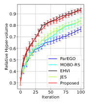
(a) $Q=2$

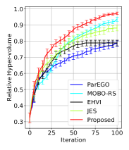
(b) $Q=3$

Figure 9: Results on parallel querying.

Appendix F Decoupled Setting

For the decoupled setting, MI and its lower bound is

$$\mathrm{MI}(f^{l}_{\boldsymbol{x}};{\cal F}^{*})$$

$$=\mathbb{E}_{{\cal F}^{*},f^{l}_{\boldsymbol{x}}}\left[\log\frac{q(f^{l}_{\boldsymbol{x}}\mid{\cal F}^{*})}{p(f^{l}_{\boldsymbol{x}})}\right]+D_{\mathrm{KL}}\left(p(f^{l}_{\boldsymbol{x}}\mid{\cal F}^{*})\parallel q(f^{l}_{\boldsymbol{x}}\mid{\cal F}^{*})\right)$$

$$\geq\mathbb{E}_{{\cal F}^{*},f^{l}_{\boldsymbol{x}}}\left[\log\frac{q(f^{l}_{\boldsymbol{x}}\mid{\cal F}^{*})}{p(f^{l}_{\boldsymbol{x}})}\right]\eqqcolon L_{\rm Dec}(\boldsymbol{x},l,\lambda).$$

We define $q(f^{l}_{\boldsymbol{x}}\mid{\cal F}^{*})$ as the marginal distribution of $q_{\lambda}(\boldsymbol{f}_{\boldsymbol{x}}\mid{\cal F}^{*})$:

$$q(f^{l}_{\boldsymbol{x}}\mid{\cal F}^{*})$$

$$=\int q_{\lambda}(\boldsymbol{f}_{\boldsymbol{x}}\mid{\cal F}^{*})\mathrm{d}\boldsymbol{f}^{-l}_{\boldsymbol{x}}$$

$$=\int\lambda q_{U}(\boldsymbol{f}_{\boldsymbol{x}}\mid{\cal F}^{*}_{S})+(1-\lambda)q_{O}(\boldsymbol{f}_{\boldsymbol{x}}\mid{\cal F}^{*}_{S})\mathrm{d}\boldsymbol{f}^{-l}_{\boldsymbol{x}}$$

$$=\int p(\boldsymbol{f}_{\boldsymbol{x}})\zeta_{\lambda}^{{\cal F}^{*}_{S}}(\boldsymbol{x})\mathbb{I}(\boldsymbol{f}_{\boldsymbol{x}}\in{\cal A}_{O}^{{\cal F}^{*}_{S}})\mathrm{d}\boldsymbol{f}^{-l}_{\boldsymbol{x}}$$

$$\qquad\qquad+\int p(\boldsymbol{f}_{\boldsymbol{x}})\eta_{\lambda}^{{\cal F}^{*}_{S}}(\boldsymbol{x})\mathbb{I}(\boldsymbol{f}_{\boldsymbol{x}}\in{\cal A}_{U\setminus O}^{{\cal F}^{*}_{S}})\mathrm{d}\boldsymbol{f}^{-l}_{\boldsymbol{x}}$$

$$=p(f^{l}_{\boldsymbol{x}})\bigl{\{}\zeta_{\lambda}^{{\cal F}^{*}_{S}}(\boldsymbol{x})\int p(\boldsymbol{f}^{-l}_{\boldsymbol{x}}\mid f^{l}_{\boldsymbol{x}})\mathbb{I}(\boldsymbol{f}_{\boldsymbol{x}}\in{\cal A}_{O}^{{\cal F}^{*}_{S}})\mathrm{d}\boldsymbol{f}^{-l}_{\boldsymbol{x}}$$

$$\qquad\qquad\qquad\qquad+\eta_{\lambda}^{{\cal F}^{*}_{S}}(\boldsymbol{x})\int p(\boldsymbol{f}^{-l}_{\boldsymbol{x}}\mid f^{l}_{\boldsymbol{x}})\mathbb{I}(\boldsymbol{f}_{\boldsymbol{x}}\in{\cal A}_{U\setminus O}^{{\cal F}^{*}_{S}})\mathrm{d}\boldsymbol{f}^{-l}_{\boldsymbol{x}}\bigr{\}}$$

$$=p(f^{l}_{\boldsymbol{x}})\bigl{\{}\zeta_{\lambda}^{{\cal F}^{*}_{S}}(\boldsymbol{x})p(\boldsymbol{f}_{\boldsymbol{x}}\in{\cal A}_{O}^{{\cal F}^{*}_{S}}\mid f^{l}_{\boldsymbol{x}})$$

$$\qquad\qquad\qquad\qquad+\eta_{\lambda}^{{\cal F}^{*}_{S}}(\boldsymbol{x})p(\boldsymbol{f}_{\boldsymbol{x}}\in{\cal A}_{U\setminus O}^{{\cal F}^{*}_{S}}\mid f^{l}_{\boldsymbol{x}})\bigr{\}},$$ (12)

where $\boldsymbol{f}_{\boldsymbol{x}}^{-l}$ is the $L-1$ dimensional subvector of $\boldsymbol{f}_{\boldsymbol{x}}$ in which $f^{l}_{\boldsymbol{x}}$ is removed. Then, the lower bound and its MC approximation is obtained as

$$L_{\rm Dec}(\boldsymbol{x},l,\lambda)$$

$$=\mathbb{E}_{{\cal F}^{*},f^{l}_{\boldsymbol{x}}}\biggl{[}\log\bigl{\{}\zeta_{\lambda}^{{\cal F}^{*}_{S}}(\boldsymbol{x})p(\boldsymbol{f}_{\boldsymbol{x}}\in{\cal A}_{O}^{{\cal F}^{*}_{S}}\mid f^{l}_{\boldsymbol{x}})$$

$$\qquad\qquad\qquad+\eta_{\lambda}^{{\cal F}^{*}_{S}}(\boldsymbol{x})p(\boldsymbol{f}_{\boldsymbol{x}}\in{\cal A}_{U\setminus O}^{{\cal F}^{*}_{S}}\mid f^{l}_{\boldsymbol{x}})\bigr{\}}\biggr{]}$$

$$\approx\frac{1}{K}\sum_{(\tilde{{\cal F}}^{*}_{S},\tilde{\boldsymbol{f}})\in F}\log\bigl{\{}\zeta_{\lambda}^{\tilde{{\cal F}}^{*}_{S}}(\boldsymbol{x})p(\boldsymbol{f}_{\boldsymbol{x}}\in{\cal A}_{O}^{\tilde{{\cal F}}^{*}_{S}}\mid\tilde{f}^{l}_{\boldsymbol{x}})$$

$$\qquad\qquad\qquad+\eta_{\lambda}^{\tilde{{\cal F}}^{*}_{S}}(\boldsymbol{x})p(\boldsymbol{f}_{\boldsymbol{x}}\in{\cal A}_{U\setminus O}^{\tilde{{\cal F}}^{*}_{S}}\mid\tilde{f}^{l}_{\boldsymbol{x}})\bigr{\}}.$$

The probabilities $p(\boldsymbol{f}_{\boldsymbol{x}}\in{\cal A}_{O}^{\tilde{{\cal F}}^{*}_{S}}\mid\tilde{f}^{l}_{\boldsymbol{x}})$ and $p(\boldsymbol{f}_{\boldsymbol{x}}\in{\cal A}_{U\setminus O}^{\tilde{{\cal F}}^{*}_{S}}\mid\tilde{f}^{l}_{\boldsymbol{x}})$ can be analytically calculated. Let ${\cal C}_{i}=(\ell_{i}^{1},u_{i}^{1}]\times(\ell_{i}^{2},u_{i}^{2}]\times\cdots\times(\ell_{i}^{L},u_{i}^{L}]$ be the cell partitions of the over truncated region ${\cal A}_{O}^{{\cal F}_{S}^{*}}$. Then, from the independence of $\boldsymbol{f}_{\boldsymbol{x}}$, we see

$$p(\boldsymbol{f}_{\boldsymbol{x}}\in{\cal A}_{O}^{\tilde{{\cal F}}^{*}_{S}}\mid\tilde{f}^{l}_{\boldsymbol{x}})$$

$$=\int p(\boldsymbol{f}^{-l}_{\boldsymbol{x}})\mathbb{I}(\boldsymbol{f}_{\boldsymbol{x}}\in{\cal A}_{O}^{\tilde{{\cal F}}^{*}_{S}})\mathrm{d}\boldsymbol{f}^{-l}_{\boldsymbol{x}}$$

$$=\sum_{c=1}^{C}\mathbb{I}(f_{\boldsymbol{x}}^{l}\in(\ell^{l}_{c},u^{l}_{c}])\int_{{\cal C}_{c}^{-l}}p(\boldsymbol{f}^{-l}_{\boldsymbol{x}})\mathrm{d}\boldsymbol{f}^{-l}_{\boldsymbol{x}}$$

$$=\sum_{c=1}^{C}\mathbb{I}(f_{\boldsymbol{x}}^{l}\in(\ell^{l}_{c},u^{l}_{c}])\prod_{l^{\prime}\neq l}\left(\Phi(\bar{\alpha}_{c,l^{\prime}})-\Phi(\underline{\alpha}_{c,l^{\prime}})\right)$$

$$=\sum_{c=1}^{C}\mathbb{I}(f_{\boldsymbol{x}}^{l}\in(\ell^{l}_{c},u^{l}_{c}])\prod_{l^{\prime}\neq l}Z_{cl^{\prime}},$$ (13)

where $Z_{cl^{\prime}}=\Phi(\bar{\alpha}_{c,l^{\prime}})-\Phi(\underline{\alpha}_{c,l^{\prime}})$ and ${\cal C}_{c}^{-l}$ is the $L-1$ dimensional hyper-rectangle created by removing the $l$-th dimension of ${\cal C}_{c}$. For $p(\boldsymbol{f}_{\boldsymbol{x}}\in{\cal A}_{U\setminus O}^{\tilde{{\cal F}}^{*}_{S}}\mid\tilde{f}^{l}_{\boldsymbol{x}})$, we use the following relation:

$$p(\boldsymbol{f}_{\boldsymbol{x}}\in{\cal A}_{U\setminus O}^{\tilde{{\cal F}}^{*}_{S}}\mid\tilde{f}^{l}_{\boldsymbol{x}})$$

$$=1-p(\boldsymbol{f}_{\boldsymbol{x}}\in{\cal A}_{O}^{\tilde{{\cal F}}^{*}_{S}}\mid\tilde{f}^{l}_{\boldsymbol{x}})-p(\boldsymbol{f}_{\boldsymbol{x}}\notin{\cal A}_{U}^{\tilde{{\cal F}}^{*}_{S}}\mid\tilde{f}^{l}_{\boldsymbol{x}}).$$

Since $\boldsymbol{f}_{\boldsymbol{x}}\notin{\cal A}_{U}^{\tilde{{\cal F}}^{*}_{S}}$ in the last term can be written as “dominated region”, shown in the end of Appendix B. We can calculate $p(\boldsymbol{f}_{\boldsymbol{x}}\notin{\cal A}_{U}^{\tilde{{\cal F}}^{*}_{S}}\mid\tilde{f}^{l}_{\boldsymbol{x}})$ by the same dominated region decomposition as (13).

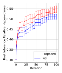
(a) $\ell_{\rm RBL}=0.05$

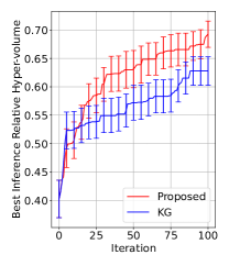
(b) $\ell_{\rm RBL}=0.1$

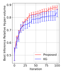
(c) $\ell_{\rm RBL}=0.25$

Figure 10: Results on decoupled setting.

Figure 10 shows the empirical evaluation for which the setting is same as in Section 6.1. Here, we used the $(d,L)=(3,3)$ GP derived functions for three length scales. As a baseline, the hypervolume-based KG is used. Since KG is defined as the hyper-volume defined by the ‘one-step ahead’ posterior mean, it is easy to extend to the decoupled setting as shown by (Daulton et al.,, 2023). To simplify the implementation, we evaluate the posterior mean hyper-volume after adding sampled $\tilde{f}^{l}(\boldsymbol{x})$ into the GPs only by using the pre-defined grid points in ${\cal X}$ (uniformly taken $5$ points in each dimension is used). For the final evaluation of the performance, since the decouple setting observes only one objective function $f^{l}(\boldsymbol{x}_{t})$ in each iteration, the hyper-volume consisting of observed points is difficult to define. Instead, we employ an approach similar to so-called inference regret. At each iteration $t$, we apply NSGA-II to the posterior mean $\boldsymbol{\mu}(\boldsymbol{x})$, and obtain a set of the Pareto optional points ${\cal X}^{*}$ for $\boldsymbol{\mu}(\boldsymbol{x})$. We evaluate the hyper-volume defined by the ground-truth objective function values on ${\cal X}^{*}$, and the plots are the maximum values of the volumes identified until each iteration. From results, we see that the decoupled extension of PFEV has reasonable performance (Note that we only have about $1/3$ observations compared with the same number of iterations of the coupled setting because only one of objective functions are observed).

Appendix G Joint Entropy Extension

Let ${\cal X}^{*}=\{\boldsymbol{x}\mid\boldsymbol{f}_{\boldsymbol{x}}\in{\cal F}^{*}\}$. The lower bound is

$$\mathrm{MI}(\boldsymbol{f}_{\boldsymbol{x}};{\cal X}^{*},{\cal F}^{*}) \geq\mathbb{E}_{{\cal X}^{*},{\cal F}^{*},\boldsymbol{f}_{\boldsymbol{x}}}\left[\log\frac{q(\boldsymbol{f}_{\boldsymbol{x}}\mid{\cal X}^{*},{\cal F}^{*})}{p(\boldsymbol{f}_{\boldsymbol{x}})}\right].$$

In practice, we only obtain a subset ${\cal X}_{S}^{*}\subseteq{\cal X}^{*}$, by which ${\cal F}_{S}^{*}=\{\boldsymbol{f}_{\boldsymbol{x}}\}_{\boldsymbol{x}\in{\cal X}_{S}^{*}}$ and ${\cal H}_{S}=\{(\boldsymbol{x},\boldsymbol{f}_{\boldsymbol{x}})\}_{\boldsymbol{x}\in{\cal X}^{*}}$ are defined. In the variational distribution $q(\boldsymbol{f}_{\boldsymbol{x}}\mid{\cal X}^{*},{\cal F}^{*})$, ${\cal H}_{S}$ can be seen as an additional training data of the GPs $\boldsymbol{f}_{\boldsymbol{x}}$. Then, a natural extension of the variational distribution (3) is

$$q_{\lambda}(\boldsymbol{f}_{\boldsymbol{x}}\mid{\cal X}^{*}_{S},{\cal F}^{*}_{S})$$

$$=\begin{cases}\left(\frac{\lambda}{Z_{U}^{{\cal F}^{*}_{S}}(\boldsymbol{x}\mid{\cal H}_{S})}+\frac{1-\lambda}{Z_{O}^{{\cal F}^{*}_{S}}(\boldsymbol{x}\mid{\cal H})}\right)p(\boldsymbol{f}_{\boldsymbol{x}}\mid{\cal H}_{S})&\text{ if }\boldsymbol{f}_{\boldsymbol{x}}\in{\cal A}_{O}^{{\cal F}^{*}_{S}},\\ \frac{\lambda}{Z_{U}^{{\cal F}^{*}_{S}}(\boldsymbol{x}\mid{\cal H}_{S})}p(\boldsymbol{f}_{\boldsymbol{x}}\mid{\cal H}_{S})&\text{ if }\boldsymbol{f}_{\boldsymbol{x}}\in{\cal A}_{U\setminus O}^{{\cal F}^{*}_{S}},\\ 0&\text{ otherwise, }\end{cases}$$

where $Z_{U}^{{\cal F}^{*}_{S}}(\boldsymbol{x}\mid{\cal H}_{S})\coloneqq p(\boldsymbol{f}_{\boldsymbol{x}}\in{\cal A}_{U}^{{\cal F}^{*}_{S}}\mid{\cal H}_{S})$ and $Z_{O}^{{\cal F}^{*}_{S}}(\boldsymbol{x}\mid{\cal H}_{S})\coloneqq p(\boldsymbol{f}_{\boldsymbol{x}}\in{\cal A}_{O}^{{\cal F}^{*}_{S}}\mid{\cal H}_{S})$. Note that here the conditioning on ${\cal H}_{S}$ is interpreted as a simple addition of the training data, and does not impose the conditions that “${\cal H}_{S}$ is the optimal solutions”, which is represented by the truncation (Because of this reason, we do not give ‘$*$’ to ${\cal H}_{S}$). The resulting lower bound is

$$\mathbb{E}_{{\cal X}^{*},{\cal F}^{*},\boldsymbol{f}_{\boldsymbol{x}}}\biggl{[}\log\bigl{\{}\zeta_{\lambda}^{{\cal F}^{*}_{S}}(\boldsymbol{x}\mid{\cal H}_{S})\mathbb{I}(\boldsymbol{f}_{\boldsymbol{x}}\in{\cal A}_{O}^{{\cal F}^{*}_{S}})$$

$$\qquad\qquad\qquad+\eta_{\lambda}^{{\cal F}^{*}_{S}}(\boldsymbol{x}\mid{\cal H}_{S})\mathbb{I}(\boldsymbol{f}_{\boldsymbol{x}}\in{\cal A}_{U\setminus O}^{{\cal F}^{*}_{S}})\bigr{\}}\biggr{]},$$ (14)

where $\zeta_{\lambda}^{{\cal F}^{*}_{S}}(\boldsymbol{x}\mid{\cal H}_{S})=\frac{\lambda}{Z_{U}^{{\cal F}^{*}_{S}}(\boldsymbol{x}\mid{\cal H}_{S})}+\frac{1-\lambda}{Z_{O}^{{\cal F}^{*}_{S}}(\boldsymbol{x}\mid{\cal H}_{S})}$ and $\eta_{\lambda}^{{\cal F}^{*}_{S}}(\boldsymbol{x}\mid{\cal H}_{S})=\frac{\lambda}{Z_{U}^{{\cal F}^{*}_{S}}(\boldsymbol{x}\mid{\cal H}_{S})}$. The same MC approximation as (6) can be used to evaluate (14).

The MAP based approximation is also possible based on transformation of (14):

$$\mathbb{E}_{{\cal X}^{*},{\cal F}^{*}}\biggl{[}p(\boldsymbol{f}_{\boldsymbol{x}}\in{\cal A}_{O}^{{\cal F}^{*}_{S}}\mid{\cal X}^{*},{\cal F}^{*})\log\zeta_{\lambda}^{{\cal F}^{*}_{S}}(\boldsymbol{x}\mid{\cal H}_{S})$$

$$\qquad\qquad\qquad+p(\boldsymbol{f}_{\boldsymbol{x}}\in{\cal A}_{U\setminus O}^{{\cal F}^{*}_{S}}\mid{\cal X}^{*},{\cal F}^{*})\log\eta_{\lambda}^{{\cal F}^{*}_{S}}(\boldsymbol{x}\mid{\cal H}_{S})\biggr{]}.$$

Based on the same idea shown in Section 3.3, we approximate $p(\boldsymbol{f}_{\boldsymbol{x}}\in{\cal A}_{O}^{{\cal F}^{*}_{S}}\mid{\cal X}^{*},{\cal F}^{*})\approx Z_{O}^{{\cal F}^{*}_{S}}(\boldsymbol{x}\mid{\cal H}_{S})/Z_{U}^{{\cal F}^{*}_{S}}(\boldsymbol{x}\mid{\cal H}_{S})$, from which the MAP estimator can be defined.

Figure 11 shows the empirical evaluation for which the setting is same as in Section 6.1. Here, we used the $(d,L)=(3,4)$ GP derived functions for three length scales. We see that the original proposed method shows slightly better performance than the JES extension, though behavior is similar each other.

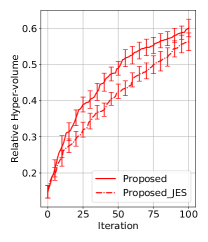
(a) $\ell_{\rm RBL}=0.05$

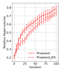
(b) $\ell_{\rm RBL}=0.1$

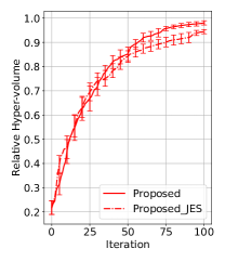
(c) $\ell_{\rm RBL}=0.25$

Figure 11: Comparison with JES extension of proposed method.

Appendix H Noisy Observation

Let $y^{l}_{\boldsymbol{x}}=f^{l}_{\boldsymbol{x}}+\varepsilon$ and $\boldsymbol{y}_{\boldsymbol{x}}=(y^{1}_{\boldsymbol{x}},\ldots,y^{L}_{\boldsymbol{x}})^{\top}$, where $\varepsilon\sim{\cal N}(0,\sigma_{\rm noise}^{2})$. The mutual information for noisy observation is $\mathrm{MI}(\boldsymbol{y}_{\boldsymbol{x}};{\cal F}^{*})$, for which the lower bound can be derived as

$$\mathrm{MI}(\boldsymbol{y}_{\boldsymbol{x}};{\cal F}^{*})$$

$$=\mathbb{E}_{{\cal F}^{*},\boldsymbol{y}_{\boldsymbol{x}}}\left[\log\frac{q(\boldsymbol{y}_{\boldsymbol{x}}\mid{\cal F}^{*})}{p(\boldsymbol{y}_{\boldsymbol{x}})}\right]$$

$$\qquad+D_{\mathrm{KL}}\left(p(\boldsymbol{y}_{\boldsymbol{x}}\mid{\cal F}^{*})\parallel q(\boldsymbol{y}_{\boldsymbol{x}}\mid{\cal F}^{*})\right)$$

$$\geq\mathbb{E}_{{\cal F}^{*},\boldsymbol{y}_{\boldsymbol{x}}}\left[\log\frac{q(\boldsymbol{y}_{\boldsymbol{x}}\mid{\cal F}^{*})}{p(\boldsymbol{y}_{\boldsymbol{x}})}\right].$$

Since ${\cal F}^{*}$ and $\boldsymbol{y}_{\boldsymbol{x}}$ are independent if $\boldsymbol{f}_{\boldsymbol{x}}$ is given, we define $q(\boldsymbol{y}_{\boldsymbol{x}}\mid{\cal F}^{*})$ by using $q_{\lambda}(\boldsymbol{f}_{\boldsymbol{x}}\mid{\cal F}^{*})$ as follows.

$$q(\boldsymbol{y}_{\boldsymbol{x}}\mid{\cal F}^{*})$$

$$=\int p(\boldsymbol{y}_{\boldsymbol{x}}\mid\boldsymbol{f}_{\boldsymbol{x}})q_{\lambda}(\boldsymbol{f}_{\boldsymbol{x}}\mid{\cal F}^{*})\mathrm{d}\boldsymbol{f}_{\boldsymbol{x}}$$

$$=\int p(\boldsymbol{y}_{\boldsymbol{x}}\mid\boldsymbol{f}_{\boldsymbol{x}})\left(\lambda q_{U}(\boldsymbol{f}_{\boldsymbol{x}}\mid{\cal F}^{*}_{S})+(1-\lambda)q_{O}(\boldsymbol{f}_{\boldsymbol{x}}\mid{\cal F}^{*}_{S})\right)\mathrm{d}\boldsymbol{f}_{\boldsymbol{x}}$$

$$=\int p(\boldsymbol{y}_{\boldsymbol{x}}\mid\boldsymbol{f}_{\boldsymbol{x}})p(\boldsymbol{f}_{\boldsymbol{x}})\bigl{\{}\zeta_{\lambda}^{{\cal F}^{*}_{S}}(\boldsymbol{x})\mathbb{I}(\boldsymbol{f}_{\boldsymbol{x}}\in{\cal A}_{O}^{{\cal F}^{*}_{S}})$$

$$\qquad\qquad+\eta_{\lambda}^{{\cal F}^{*}_{S}}(\boldsymbol{x})\mathbb{I}(\boldsymbol{f}_{\boldsymbol{x}}\in{\cal A}_{U\setminus O}^{{\cal F}^{*}_{S}})\bigr{\}}\mathrm{d}\boldsymbol{f}_{\boldsymbol{x}}$$

$$=\int_{\boldsymbol{f}_{\boldsymbol{x}}\in{\cal A}_{O}^{{\cal F}^{*}_{S}}}p(\boldsymbol{y}_{\boldsymbol{x}},\boldsymbol{f}_{\boldsymbol{x}})\zeta_{\lambda}^{{\cal F}^{*}_{S}}(\boldsymbol{x})\mathrm{d}\boldsymbol{f}_{\boldsymbol{x}}$$

$$\qquad\qquad+\int_{\boldsymbol{f}_{\boldsymbol{x}}\in{\cal A}_{U\setminus O}^{{\cal F}^{*}_{S}}}p(\boldsymbol{y}_{\boldsymbol{x}},\boldsymbol{f}_{\boldsymbol{x}})\eta_{\lambda}^{{\cal F}^{*}_{S}}(\boldsymbol{x})\mathrm{d}\boldsymbol{f}_{\boldsymbol{x}}$$

$$=p(\boldsymbol{y}_{\boldsymbol{x}})\biggl{\{}\zeta_{\lambda}^{{\cal F}^{*}_{S}}(\boldsymbol{x})\int_{\boldsymbol{f}_{\boldsymbol{x}}\in{\cal A}_{O}^{{\cal F}^{*}_{S}}}p(\boldsymbol{f}_{\boldsymbol{x}}\mid\boldsymbol{y}_{\boldsymbol{x}})\mathrm{d}\boldsymbol{f}_{\boldsymbol{x}}$$

$$\qquad\qquad+\eta_{\lambda}^{{\cal F}^{*}_{S}}(\boldsymbol{x})\int_{\boldsymbol{f}_{\boldsymbol{x}}\in{\cal A}_{U\setminus O}^{{\cal F}^{*}_{S}}}p(\boldsymbol{f}_{\boldsymbol{x}}\mid\boldsymbol{y}_{\boldsymbol{x}})\mathrm{d}\boldsymbol{f}_{\boldsymbol{x}}\biggr{\}}$$

$$=p(\boldsymbol{y}_{\boldsymbol{x}})\left\{\zeta_{\lambda}^{{\cal F}^{*}_{S}}(\boldsymbol{x})p(\boldsymbol{f}_{\boldsymbol{x}}\in{\cal A}_{O}^{{\cal F}^{*}_{S}}\mid\boldsymbol{y}_{\boldsymbol{x}})\right.$$

$$\qquad\qquad\left.+\eta_{\lambda}^{{\cal F}^{*}_{S}}(\boldsymbol{x})p(\boldsymbol{f}_{\boldsymbol{x}}\in{\cal A}_{U\setminus O}^{{\cal F}^{*}_{S}}\mid\boldsymbol{y}_{\boldsymbol{x}})\right\}.$$

Then, the MC approximation becomes

$$\mathbb{E}_{{\cal F}^{*},\boldsymbol{y}_{\boldsymbol{x}}}\left[\log\left\{\zeta_{\lambda}^{{\cal F}^{*}_{S}}(\boldsymbol{x})p(\boldsymbol{f}_{\boldsymbol{x}}\in{\cal A}_{O}^{{\cal F}^{*}_{S}}\mid\boldsymbol{y}_{\boldsymbol{x}})\right.\right.$$

$$\qquad\left.\left.+\eta_{\lambda}^{{\cal F}^{*}_{S}}(\boldsymbol{x})p(\boldsymbol{f}_{\boldsymbol{x}}\in{\cal A}_{U\setminus O}^{{\cal F}^{*}_{S}}\mid\boldsymbol{y}_{\boldsymbol{x}})\right\}\right]$$

$$\approx\frac{1}{KK_{\varepsilon}}\sum_{(\tilde{{\cal F}}^{*}_{S},\tilde{\boldsymbol{f}})\in F}\sum_{\tilde{\varepsilon}\in E}\log\left\{\zeta_{\lambda}^{\tilde{{\cal F}}^{*}_{S}}(\boldsymbol{x})p(\boldsymbol{f}_{\boldsymbol{x}}\in{\cal A}_{O}^{\tilde{{\cal F}}^{*}_{S}}\mid\tilde{\boldsymbol{y}}_{\boldsymbol{x}})\right.$$

$$\qquad\left.+\eta_{\lambda}^{\tilde{{\cal F}}^{*}_{S}}(\boldsymbol{x})p(\boldsymbol{f}_{\boldsymbol{x}}\in{\cal A}_{U\setminus O}^{\tilde{{\cal F}}^{*}_{S}}\mid\tilde{\boldsymbol{y}}_{\boldsymbol{x}})\right\}.$$

where $E$ is a set of $L$-dimension noise samples $\tilde{\varepsilon}$ from ${\cal N}(0,\sigma^{2}_{\rm noise}I)$, $\tilde{\boldsymbol{y}}_{\boldsymbol{x}}=\tilde{\boldsymbol{f}}_{\boldsymbol{x}}+\tilde{\varepsilon}$ is a sample of $\boldsymbol{y}_{\boldsymbol{x}}$, and $K_{\varepsilon}=|E|$. Note that, in this approximation, we transform $\mathbb{E}_{{\cal F}^{*},\boldsymbol{y}_{\boldsymbol{x}}}$ to $\mathbb{E}_{{\cal F}^{*},\boldsymbol{f}_{\boldsymbol{x}}}\mathbb{E}_{\boldsymbol{\varepsilon}}$, which is possible because of the independence of the noise term. To evaluate this MC approximation, we need the conditional distribution $p(\boldsymbol{f}_{\boldsymbol{x}}\mid\tilde{\boldsymbol{y}}_{\boldsymbol{x}})$, written as

$$\boldsymbol{f}_{\boldsymbol{x}}\mid\tilde{\boldsymbol{y}}_{\boldsymbol{x}}\sim{\cal N}(\boldsymbol{\nu}(\boldsymbol{x}),\mathrm{diag}(\boldsymbol{s}(\boldsymbol{x}))),$$

where

$$\nu_{l}(\boldsymbol{x}) =\mu_{l}(\boldsymbol{x})+\frac{\sigma_{l}^{2}(\boldsymbol{x})}{\sigma_{l}^{2}(\boldsymbol{x})+\sigma_{\rm noise}^{2}}(\tilde{y}^{l}_{\boldsymbol{x}}-\mu_{l}(\boldsymbol{x})),$$

$$s_{l}(\boldsymbol{x}) =\sigma_{l}^{2}(\boldsymbol{x})-\frac{\sigma_{l}^{4}(\boldsymbol{x})}{\sigma_{l}^{2}(\boldsymbol{x})+\sigma_{\rm noise}^{2}}.$$

Therefore, $p(\boldsymbol{f}_{\boldsymbol{x}}\in{\cal A}_{O}^{\tilde{{\cal F}}^{*}_{S}}\mid\tilde{\boldsymbol{y}}_{\boldsymbol{x}})$ can be calculated by using the same procedure as $Z_{O}^{\tilde{{\cal F}}^{*}_{S}}=p(\boldsymbol{f}_{\boldsymbol{x}}\in{\cal A}_{O}^{\tilde{{\cal F}}^{*}_{S}})$ shown in (9):

$$p(\boldsymbol{f}_{\boldsymbol{x}}\in{\cal A}_{O}^{\tilde{{\cal F}}^{*}_{S}}\mid\tilde{\boldsymbol{y}}_{\boldsymbol{x}}) =\sum_{i=1}^{C}\int_{C_{i}}p(\boldsymbol{f}_{\boldsymbol{x}}\mid\tilde{\boldsymbol{y}}_{\boldsymbol{x}})\mathrm{d}\boldsymbol{f}_{\boldsymbol{x}}$$

$$=\sum_{i=1}^{C}\prod_{l=1}^{L}\int_{\ell_{i}^{l}}^{u_{i}^{l}}p(f^{l}_{\boldsymbol{x}}\mid\tilde{y}^{l}_{\boldsymbol{x}})\mathrm{d}f^{l}_{\boldsymbol{x}}$$

$$=\sum_{i=1}^{C}\prod_{l=1}^{L}\left(\Phi(\bar{\beta}_{i,l})-\Phi(\underline{\beta}_{i,l})\right)$$

where $\underline{\beta}_{i,l}=(\ell_{i}^{l}-\nu_{l}(\boldsymbol{x}))/s_{l}(\boldsymbol{x})$ and $\bar{\beta}_{i,l}=(u_{i}^{l}-\nu_{l}(\boldsymbol{x}))/s_{l}(\boldsymbol{x})$. For $p(\boldsymbol{f}_{\boldsymbol{x}}\in{\cal A}_{U\setminus O}^{\tilde{{\cal F}}^{*}_{S}}\mid\tilde{\boldsymbol{y}}_{\boldsymbol{x}})$, we can use a relation $p(\boldsymbol{f}_{\boldsymbol{x}}\in{\cal A}_{U\setminus O}^{\tilde{{\cal F}}^{*}_{S}}\mid\tilde{\boldsymbol{y}}_{\boldsymbol{x}})=p(\boldsymbol{f}_{\boldsymbol{x}}\in{\cal A}_{U}^{\tilde{{\cal F}}^{*}_{S}}\mid\tilde{\boldsymbol{y}}_{\boldsymbol{x}})-p(\boldsymbol{f}_{\boldsymbol{x}}\in{\cal A}_{O}^{\tilde{{\cal F}}^{*}_{S}}\mid\tilde{\boldsymbol{y}}_{\boldsymbol{x}})$. The last term $p(\boldsymbol{f}_{\boldsymbol{x}}\in{\cal A}_{O}^{\tilde{{\cal F}}^{*}_{S}}\mid\tilde{\boldsymbol{y}}_{\boldsymbol{x}})$ can be calculated by the same approach as $Z_{U}^{\tilde{{\cal F}}^{*}_{S}}=p(\boldsymbol{f}_{\boldsymbol{x}}\in{\cal A}_{U}^{\tilde{{\cal F}}^{*}_{S}})$, described in the end of Appendix B.

Figure 12 shows the empirical evaluation for which the setting is same as in Section 6.1. Here, we used the $(d,L)=(3,3)$ GP derived functions for three length scales. We added the independent noise ${\cal N}(0,\sigma_{\rm noise}^{2})$ with $\sigma_{\rm noise}=0.1$ to all the observations. The GPs have the same value of the noise parameter $\sigma_{\rm noise}=0.1$. We compared with EHVI, MOBO-RS, and JES. EHVI and MOBO-RS can handle the noise just by incorporating it into the surrogate GPs. JES (Tu et al.,, 2022) considers the information gain from noisy observations. PFEV shows similar results to its noisy observation counterpart. We empirically see that $\mathrm{MI}(\boldsymbol{f}(\boldsymbol{x});{\cal F}^{*})$ sufficiently works even when the observation contains moderate level of the noise. The investigation under stronger noise is our future work.

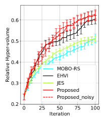
(a) $\ell_{\rm RBL}=0.05$

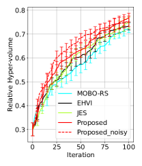
(b) $\ell_{\rm RBL}=0.1$

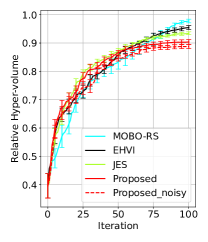
(c) $\ell_{\rm RBL}=0.25$

Figure 12: Results with noisy observations in GP-derived synthetic functions (average and standard error of $10$ runs)

Appendix I Additional Discussion on Related Work

Although our main focus is on information theoretic approaches, here, other criteria are also reviewed. A classical approach is the scalarization that transforms multiple objective functions into a scalar value, among which ParEGO (Knowles,, 2006) is a well-known method based on a random scalarization. However, the information of the Pareto-frontier may be lost by the scalarization. The standard expected improvement (EI) has been extended based on measuring the improvement of the hyper-volume called EHVI (expected hyper-volume improvement) (Emmerich,, 2005; Shah and Ghahramani,, 2016). The GP upper confidence bound (UCB) is another well-known general approach to BO (Srinivas et al.,, 2010). UCB based MOBO methods have been studied (Ponweiser et al.,, 2008; Zuluaga et al.,, 2013, 2016), but the setting of the confidence interval sometimes becomes practically difficult. SUR (Picheny,, 2015) is based on the reduction of PI after the querying, which is computationally quite expensive. A hypervolume-based multi-objective extension of knowledge gradient (KG) is considered by (Daulton et al.,, 2023). Naïve computations of the hypervolume KG is computationally intractable, and several approximation and acceleration strategies have been studied. For example, so-called one-shot strategy transforms the nested optimization into simultaneous optimization which makes computation much faster, but the dimension of the acquisition function optimization becomes high.

We focus on the information-theoretic approach, which was first proposed for single objective BO (Hennig and Schuler,, 2012; Hernández-Lobato et al.,, 2014; Wang and Jegelka,, 2017). Recently, (Cheng and Becker,, 2024) proposed a different variational lower bound approach to single objective BO, which is only for single objective problems. A seminal work in the information-theoretic approach to MOBO is the Predictive Entropy Search for Multi-Objective Optimization (PESMO) (Hernandez-Lobato et al.,, 2016). PESMO defines an acquisition function through the entropy of the set of Pareto-optimal solutions $\boldsymbol{x}$, which is based on complicated approximation by expectation propagation (EP) (Minka,, 2001). On the other hand, Belakaria et al., (2019) proposed using the individual max-value entropy of each objective function, called max-value entropy search for multi-objective optimization (MESMO). This largely simplifies the computations, but obviously, information of the Pareto-frontier is lost. Another JES based approach has been recently proposed (Fernández-Sánchez and Hernández-Lobato,, 2024), which is in a more general formulation including multi-fidelity and constrained problems. Their computations are based on the Gaussian based entropy approximation, whose validity remains unclear.

Appendix J Detail of Experimental Settings

Bayesian optimization was implemented by a Python package called GPy (GPy,, 2012). PFEV, PFES, and $\{\text{PF}\}^{2}\text{ES}$ requires ${\cal C}_{i}$ that are hyper-rectangles decomposing the dominated region. To obtain ${\cal C}_{i}$, we used Quick Hyper-volume (QHV) (Russo and Francisco,, 2014), which is an efficient recursive algorithm originally proposed for the Pareto hyper-volume calculation. In PFEV, we maximize $\lambda$ for each given $\boldsymbol{x}$ by calculating $\widehat{L}(\boldsymbol{x},\lambda)$ for $11$ grid points of $\lambda$ ($10^{-3},0.1,0.2,\ldots,1.0$). In RFM used for sampling ${\cal F}^{*}$ (required in PFEV, PFES, MESMO, $\{\text{PF}\}^{2}\text{ES}$, and JES), the number of basis $D$ was $500$. The GP hyper-parameter $\sigma^{2}_{\rm noise}$ is fixed as $10^{-4}$. In ParEGO, the coefficient parameter in the augmented Tchebycheff function was set $0.05$ as shown in (Knowles,, 2006).

The definition of each benchmark function is as follows.

• Fonseca-Fleming (Fonseca and Fleming,, 1995)

  $$f_{1}(\boldsymbol{x}) =1-\exp\left[-\sum_{i=1}^{d}\left(x_{i}-\frac{1}{\sqrt{d}}\right)^{2}\right]$$

  $$f_{2}(\boldsymbol{x}) =1-\exp\left[-\sum_{i=1}^{d}\left(x_{i}+\frac{1}{\sqrt{d}}\right)^{2}\right]$$

  subject to $$\quad-4\leq x_{i}\leq 4,\quad i\in[d].$$

• Kursawe (Kursawe,, 1990)

  $$f_{1}(\boldsymbol{x}) =\sum_{i=1}^{2}\left[-10\exp\left(-0.2\sqrt{x_{i}^{2}+x_{i+1}^{2}}\right)\right]$$

  $$f_{2}(\boldsymbol{x}) =\sum_{i=1}^{3}\left[|x_{i}|^{0.8}+5\sin(x_{i}^{3})\right]$$

  subject to $$\quad-5\leq x_{i}\leq 5,\quad 1\leq i\leq 3.$$

• Viennet (Vlennet et al.,, 1996)

  $$f_{1}(x,y) =0.5\left(x^{2}+y^{2}\right)+\sin\left(x^{2}+y^{2}\right)$$

  $$f_{2}(x,y) =\frac{(3x-2y+4)^{2}}{8}+\frac{(x-y+1)^{2}}{27}+15$$

  $$f_{3}(x,y) =\frac{1}{x^{2}+y^{2}+1}-1.1\exp\left(-(x^{2}+y^{2})\right)$$

  subject to $$\quad-3\leq x,y\leq 3.$$

• FES1 (Fieldsend et al.,, 2003)

  $$f_{1}(\boldsymbol{x}) =\sum_{i=1}^{d}\left|x_{i}-\exp\left(\frac{(i/d)^{2}}{3}\right)\right|^{0.5}$$

  $$f_{2}(\boldsymbol{x}) =\sum_{i=1}^{d}\left(x_{i}-0.5\cos\left(\frac{10\pi i}{d}\right)-0.5\right)^{2}$$

  subject to $$\quad 0\leq x_{i}\leq 1,\quad i\in[d].$$

• FES2 (Fieldsend et al.,, 2003)

  $$f_{1}(\boldsymbol{x}) =\sum_{i=1}^{d}\left(x_{i}-0.5\cos\left(\frac{10\pi i}{d}\right)-0.5\right)^{2}$$

  $$f_{2}(\boldsymbol{x}) =\sum_{i=1}^{d}\left|x_{i}-\sin^{2}(i-1)\cos^{2}(i-1)\right|^{0.5}$$

  $$f_{3}(\boldsymbol{x}) =\sum_{i=1}^{d}\left|x_{i}-0.25\cos(i-1)\cos(2i-2)-0.5\right|^{0.5}$$

  subject to $$\quad 0\leq x_{i}\leq 1,\quad i\in[d].$$

• FES3 (Fieldsend et al.,, 2003)

  $$f_{1}(\boldsymbol{x}) =-\sum_{i=1}^{d}\left|x_{i}-\frac{\exp\left(\left(\frac{i}{d}\right)^{2}\right)}{3}\right|^{0.5},$$

  $$f_{2}(\boldsymbol{x}) =-\sum_{i=1}^{d}\left|x_{i}-\sin(i-1)^{2}\cos(i-1)^{2}\right|^{0.5},$$

  $$f_{3}(\boldsymbol{x}) =-\sum_{i=1}^{d}\left|x_{i}-\left(0.25\cos(i-1)\cos(2i-1)-0.5\right)\right|^{0.5},$$

  $$f_{4}(\boldsymbol{x}) =-\sum_{i=1}^{d}\left(x_{i}-\frac{1}{2}\sin\left(1000\pi\frac{i}{d}\right)-\frac{1}{2}\right)^{2}$$

  subject to $$\quad 0\leq x_{i}\leq 1,\quad i\in[d].$$

Appendix K Additional Results of Empirical Evaluation

K.1 Additional Results on GP-derived Synthetic Functions

Additional results on GP-derived synthetic functions are shown in Fig. 13-15. The results are all combinations of $\ell_{\rm RBF}\in\{0.05,0.1,0.25\}$, $L\in\{2,3,4,5,6\}$, and $d\in\{2,3,4\}$ (Note that $\ell_{\rm RBF}=0.1$ in $d\in\{2,3\}$ is the same results as the main text). The boxplots created from all the results is shown in Fig. 16.

Further, Fig. 17 is performance difference between Bayes MAP (8) and naïve MC (6).

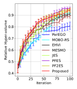
(a) $(L,\ell_{\rm RBF})=(2,0.05)$

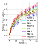
(b) $(L,\ell_{\rm RBF})=(3,0.05)$

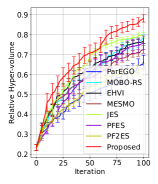
(c) $(L,\ell_{\rm RBF})=(4,0.05)$

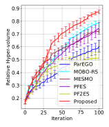
(d) $(L,\ell_{\rm RBF})=(5,0.05)$

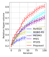
(e) $(L,\ell_{\rm RBF})=(6,0.05)$

(f) $(L,\ell_{\rm RBF})=(2,0.1)$

(g) $(L,\ell_{\rm RBF})=(3,0.1)$

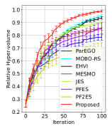
(h) $(L,\ell_{\rm RBF})=(4,0.1)$

(i) $(L,\ell_{\rm RBF})=(5,0.1)$

(j) $(L,\ell_{\rm RBF})=(6,0.1)$

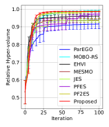
(k) $(L,\ell_{\rm RBF})=(2,0.25)$

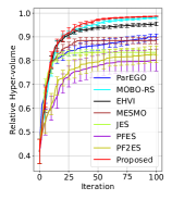
(l) $(L,\ell_{\rm RBF})=(3,0.25)$

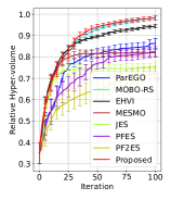
(m) $(L,\ell_{\rm RBF})\!=\!(4,0.25)$

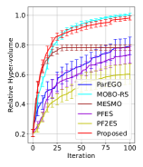
(n) $(L,\ell_{\rm RBF})=(5,0.25)$

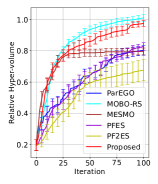
(o) $(L,\ell_{\rm RBF})=(6,0.25)$

Figure 13: Results on GP-derived synthetic function ($d=2$)

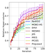
(a) $(L,\ell_{\rm RBF})=(2,0.05)$

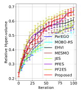
(b) $(L,\ell_{\rm RBF})=(3,0.05)$

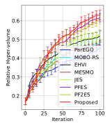
(c) $(L,\ell_{\rm RBF})=(4,0.05)$

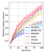
(d) $(L,\ell_{\rm RBF})=(5,0.05)$

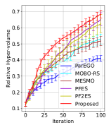
(e) $(L,\ell_{\rm RBF})=(6,0.05)$

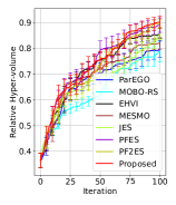
(f) $(L,\ell_{\rm RBF})=(2,0.1)$

(g) $(L,\ell_{\rm RBF})=(3,0.1)$

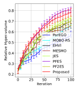
(h) $(L,\ell_{\rm RBF})=(4,0.1)$

(i) $(L,\ell_{\rm RBF})=(5,0.1)$

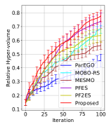
(j) $(L,\ell_{\rm RBF})=(6,0.1)$

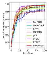
(k) $(L,\ell_{\rm RBF})=(2,0.25)$

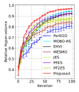
(l) $(L,\ell_{\rm RBF})=(3,0.25)$

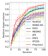
(m) $(L,\ell_{\rm RBF})\!=\!(4,0.25)$

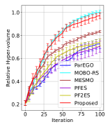
(n) $(L,\ell_{\rm RBF})=(5,0.25)$

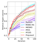
(o) $(L,\ell_{\rm RBF})=(6,0.25)$

Figure 14: Results on GP-derived synthetic function ($d=3$)

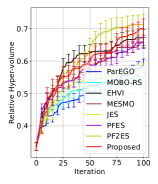
(a) $(L,\ell_{\rm RBF})=(2,0.05)$

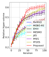
(b) $(L,\ell_{\rm RBF})=(3,0.05)$

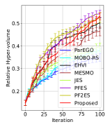
(c) $(L,\ell_{\rm RBF})=(4,0.05)$

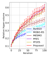
(d) $(L,\ell_{\rm RBF})=(5,0.05)$

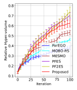
(e) $(L,\ell_{\rm RBF})=(6,0.05)$

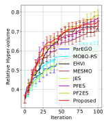
(f) $(L,\ell_{\rm RBF})=(2,0.1)$

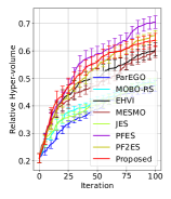
(g) $(L,\ell_{\rm RBF})=(3,0.1)$

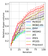
(h) $(L,\ell_{\rm RBF})=(4,0.1)$

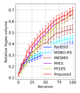
(i) $(L,\ell_{\rm RBF})=(5,0.1)$

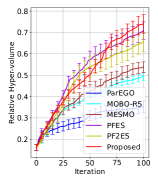
(j) $(L,\ell_{\rm RBF})=(6,0.1)$

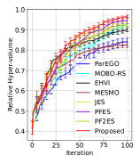
(k) $(L,\ell_{\rm RBF})=(2,0.25)$

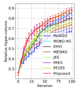
(l) $(L,\ell_{\rm RBF})=(3,0.25)$

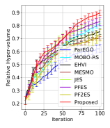
(m) $(L,\ell_{\rm RBF})\!=\!(4,0.25)$

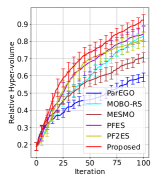
(n) $(L,\ell_{\rm RBF})=(5,0.25)$

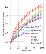
(o) $(L,\ell_{\rm RBF})=(6,0.25)$

Figure 15: Results on GP-derived synthetic function ($d=4$)

(a) $L=2$

(b) $L=3$

(c) $L=4$

(d) $L=5$

(e) $L=6$

Figure 16: Boxplots of RHV at $100$-th iteration.

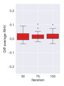
Figure 17: Boxplot of difference of average RHV between Bayes MAP and naïve MC (Bayes MAP minus naïve MC). The differences of the $10$ runs average RHV are shown for BO iterations $50$, $75$, and $100$. The GP-derived functions of $d\in\{2,3,4\}$, $L\in\{2,3,4\}$, and $\ell_{\rm RBF}\in\{0.05,0.1,0.25\}$ were used (i.e., $27=3\times 3\times 3$ points for each iteration). Since positive values indicate Bayes MAP is better than naïve MC, we see that Bayes MAP shows slightly better performance across iterations.

K.2 Additional Results on Benchmark Functions

Figure 18 show additional results on benchmark functions. FES1 and FES2 are $(d,L)=(3,2)$ and $(d,L)=(3,3)$, respectively. Therefore, FES1$+$Kursawe and FES2$+$Kursawe are $(d,L)=(3,4)$ and $(d,L)=(3,5)$, respectively. Further, Figure 19 shows the results on higher dimensional input setting ($d=10$) of FES1, FES2, and FES3.

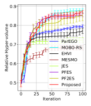
(a) FES1

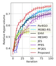
(b) FES2

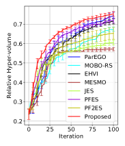
(c) FES1$+$Kursawe

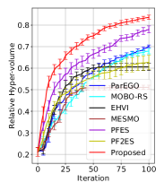
(d) FES2$+$Kursawe

Figure 18: Performance comparison in benchmark functions (average and standard deviation of $10$ runs).

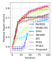
(a) FES1-10

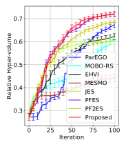
(b) FES2-10

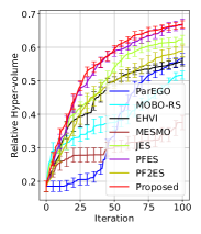
(c) FES3-10

Figure 19: Performance comparison in benchmark functions (average and standard deviation of $10$ runs).

K.3 Computational Time

We here examine the computational time of PFEV. We used the GP-derived synthetic function ($d=3$) from Section 6.1. The training dataset was randomly selected $50$ points, and we evaluated the computational time (CPU time) required to calculate the acquisition function values for $100$ points generated by the Latin hyper cube sampling. In PFEV, we evaluate time of calculating $11$ grid points of $\lambda$ ($10^{-3},0.1,0.2,\ldots,1.0$) for a given $\boldsymbol{x}$. The results are shown in Table 1, in which we evaluate ParEGO, PFES, EHVI, and PFEV (Proposed).

Obviously, ParEGO was quite fast because it applies the usual single objective BO to the scalarized value. For $L=3$ and $4$, EHVI was also fast, but it becomes slow at $L=5$ and we stopped it at $L=6$ because of the long computational time. The slow computation of EHVI at large $L$ is widely known. PFEV and PFES were similar up to $L=4$, but for $L=5$ and $L=6$, PFEV was slower than PFES. This is because of the computation of QHV. For $L=3$ and $L=4$, the computational time of NSGAII was dominant in PFEV (Note that the same procedure is also performed in PFES). However, for $L=5$, QHV requires the similar cost as NSGAII, and for $L=6$, the computational cost of QHV became much larger than NSGAII. PFEV requires QHV two times for each sampled Pareto-frontier (see Appendix B) while PFES requires QHV only once for each sampled Pareto-frontier. This was major reason of the difference of PFEV and PFES in $L=6$.

Table 1: CPU time evaluation (sec).

		$L=3$	$L=4$	$L=5$	$L=6$
ParEGO		0.95 $\pm$ 0.08	1.15 $\pm$ 0.06	1.38 $\pm$ 0.07	1.62 $\pm$ 0.11
PFES		21.43 $\pm$ 0.20	29.18 $\pm$ 0.39	45.23 $\pm$ 1.41	127.64 $\pm$ 24.44
EHVI		0.86 $\pm$ 0.06	3.51 $\pm$ 2.24	500.09 $\pm$ 336.18	-
Proposed	Total	21.93 $\pm$ 0.42	31.74 $\pm$ 0.64	61.04 $\pm$ 3.26	274.49 $\pm$ 28.99
	CalcPFEV	0.59 $\pm$ 0.05	1.56 $\pm$ 0.13	5.04 $\pm$ 0.49	24.76 $\pm$ 3.71
	NSGAII	19.59 $\pm$ 0.37	25.66 $\pm$ 0.37	31.36 $\pm$ 0.27	37.26 $\pm$ 0.22
	RFM	0.59 $\pm$ 0.00	0.80 $\pm$ 0.01	1.00 $\pm$ 0.00	1.19 $\pm$ 0.00
	QHV	0.42 $\pm$ 0.03	2.72 $\pm$ 0.26	22.41 $\pm$ 2.65	209.81 $\pm$ 25.68

References

- Belakaria et al., (2019) Belakaria, S., Deshwal, A., and Doppa, J. R. (2019). Max-value entropy search for multi-objective bayesian optimization. Advances in neural information processing systems, 32.
- Bishop and Bishop, (2023) Bishop, C. M. and Bishop, H. (2023). Deep learning: Foundations and concepts. Springer Nature.
- Cheng and Becker, (2024) Cheng, N. and Becker, S. (2024). Variational entropy search for adjusting expected improvement. arXiv:2402.11345.
- Cover and Thomas, (2006) Cover, T. M. and Thomas, J. A. (2006). Elements of Information Theory. Wiley-Interscience.
- Daulton et al., (2023) Daulton, S., Balandat, M., and Bakshy, E. (2023). Hypervolume knowledge gradient: A lookahead approach for multi-objective Bayesian optimization with partial information. In Proceedings of the 40th International Conference on Machine Learning, volume 202 of Proceedings of Machine Learning Research, pages 7167–7204. PMLR.
- Deb et al., (2002) Deb, K., Pratap, A., Agarwal, S., and Meyarivan, T. (2002). A fast and elitist multiobjective genetic algorithm: NSGA-II. IEEE Transactions on Evolutionary Computation, 6(2):182–197.
- Emmerich, (2005) Emmerich, M. T. (2005). Single-and multi-objective evolutionary design optimization assisted by gaussian random field metamodels. PhD thesis, Dortmund University, Germany.
- Fernández-Sánchez and Hernández-Lobato, (2024) Fernández-Sánchez, D. and Hernández-Lobato, D. (2024). Joint entropy search for multi-objective bayesian optimization with constraints and multiple fidelities. In ESANN 2024 proceedings, European Symposium on Artificial Neural Networks, Computational Intelligence and Machine Learning.
- Fieldsend et al., (2003) Fieldsend, J. E., Everson, R. M., and Singh, S. (2003). Using unconstrained elite archives for multiobjective optimization. IEEE Transactions on Evolutionary Computation, 7(3):305–323.
- Fonseca and Fleming, (1995) Fonseca, C. M. and Fleming, P. J. (1995). Multiobjective genetic algorithms made easy: selection sharing and mating restriction. In First International Conference on Genetic Algorithms in Engineering Systems: Innovations and Applications, pages 45–52. IET.
- GPy, (2012) GPy (since 2012). GPy: A Gaussian process framework in python. http://github.com/SheffieldML/GPy.
- Hennig and Schuler, (2012) Hennig, P. and Schuler, C. J. (2012). Entropy search for information-efficient global optimization. Journal of Machine Learning Research, 13(57):1809–1837.
- Hernandez-Lobato et al., (2016) Hernandez-Lobato, D., Hernandez-Lobato, J., Shah, A., and Adams, R. (2016). Predictive entropy search for multi-objective Bayesian optimization. In Proceedings of The 33rd International Conference on Machine Learning, volume 48, pages 1492–1501. PMLR.
- Hernández-Lobato et al., (2014) Hernández-Lobato, J. M., Hoffman, M. W., and Ghahramani, Z. (2014). Predictive entropy search for efficient global optimization of black-box functions. In Advances in Neural Information Processing Systems 27, page 918–926. Curran Associates, Inc.
- Jones et al., (1993) Jones, D. R., Perttunen, C. D., and Stuckman, B. E. (1993). Lipschitzian optimization without the lipschitz constant. Journal of Optimization Theory and Applications, 79(1):157–181.
- Kandasamy et al., (2018) Kandasamy, K., Krishnamurthy, A., Schneider, J., and Póczos, B. (2018). Parallelised Bayesian optimisation via Thompson sampling. In Proceedings of the 21st International Conference on Artificial Intelligence and Statistics, volume 84, pages 133–142. PMLR.
- Knowles, (2006) Knowles, J. (2006). ParEGO: A hybrid algorithm with on-line landscape approximation for expensive multiobjective optimization problems. IEEE transactions on evolutionary computation, 10(1):50–66.
- Kursawe, (1990) Kursawe, F. (1990). A variant of evolution strategies for vector optimization. In International conference on parallel problem solving from nature, pages 193–197. Springer.
- Minka, (2001) Minka, T. P. (2001). Expectation propagation for approximate Bayesian inference. In Proceedings of the 17th Conference in Uncertainty in Artificial Intelligence, pages 362–369. Morgan Kaufmann Publishers Inc.
- Paria et al., (2020) Paria, B., Kandasamy, K., and Póczos, B. (2020). A flexible framework for multi-objective bayesian optimization using random scalarizations. In Uncertainty in Artificial Intelligence, pages 766–776. PMLR.
- Perrone et al., (2019) Perrone, V., Shcherbatyi, I., Jenatton, R., Archambeau, C., and Seeger, M. (2019). Constrained Bayesian optimization with max-value entropy search. arXiv:1910.07003.
- Picheny, (2015) Picheny, V. (2015). Multiobjective optimization using gaussian process emulators via stepwise uncertainty reduction. Statistics and Computing, 25(6):1265–1280.
- Ponweiser et al., (2008) Ponweiser, W., Wagner, T., Biermann, D., and Vincze, M. (2008). Multiobjective optimization on a limited budget of evaluations using model-assisted-metric selection. In International conference on parallel problem solving from nature, pages 784–794. Springer.
- Qing et al., (2022) Qing, J., Moss, H. B., Dhaene, T., and Couckuyt, I. (2022). PF ES: Parallel feasible pareto frontier entropy search for multi-objective bayesian optimization. arXiv preprint arXiv:2204.05411.
- Rahimi and Recht, (2008) Rahimi, A. and Recht, B. (2008). Random features for large-scale kernel machines. In Advances in Neural Information Processing Systems 20, pages 1177–1184. Curran Associates, Inc.
- Russo and Francisco, (2014) Russo, L. M. and Francisco, A. P. (2014). Quick hypervolume. IEEE Transactions on Evolutionary Computation, 4(18):481–502.
- Shah and Ghahramani, (2016) Shah, A. and Ghahramani, Z. (2016). Pareto frontier learning with expensive correlated objectives. In International conference on machine learning, pages 1919–1927. PMLR.
- Shahriari et al., (2016) Shahriari, B., Swersky, K., Wang, Z., Adams, R., and De Freitas, N. (2016). Taking the human out of the loop: A review of Bayesian optimization. Proceedings of the IEEE, 104(1):148–175.
- Srinivas et al., (2010) Srinivas, N., Krause, A., Kakade, S., and Seeger, M. (2010). Gaussian process optimization in the bandit setting: No regret and experimental design. In Proceedings of the 27th International Conference on International Conference on Machine Learning, pages 1015–1022. Omnipress.
- Suzuki et al., (2020) Suzuki, S., Takeno, S., Tamura, T., Shitara, K., and Karasuyama, M. (2020). Multi-objective Bayesian optimization using Pareto-frontier entropy. In Proceedings of the 37th International Conference on Machine Learning, volume 119, pages 9279–9288. PMLR.
- Takeno et al., (2020) Takeno, S., Fukuoka, H., Tsukada, Y., Koyama, T., Shiga, M., Takeuchi, I., and Karasuyama, M. (2020). Multi-fidelity Bayesian optimization with max-value entropy search and its parallelization. In Proceedings of the 37th International Conference on Machine Learning, volume 119, pages 9334–9345. PMLR.
- Takeno et al., (2022) Takeno, S., Tamura, T., Shitara, K., and Karasuyama, M. (2022). Sequential and parallel constrained max-value entropy search via information lower bound. In Proceedings of the 39th International Conference on Machine Learning, volume 162 of Proceedings of Machine Learning Research, pages 20960–20986. PMLR.
- Tu et al., (2022) Tu, B., Gandy, A., Kantas, N., and Shafei, B. (2022). Joint entropy search for multi-objective bayesian optimization. Advances in Neural Information Processing Systems, 35:9922–9938.
- Vlennet et al., (1996) Vlennet, R., Fonteix, C., and Marc, I. (1996). Multicriteria optimization using a genetic algorithm for determining a pareto set. International Journal of Systems Science, 27(2):255–260.
- Wang and Jegelka, (2017) Wang, Z. and Jegelka, S. (2017). Max-value entropy search for efficient Bayesian optimization. In Proceedings of the 34th International Conference on Machine Learning, volume 70, pages 3627–3635. PMLR.
- Zuluaga et al., (2016) Zuluaga, M., Krause, A., et al. (2016). e-pal: An active learning approach to the multi-objective optimization problem. Journal of Machine Learning Research, 17(104):1–32.
- Zuluaga et al., (2013) Zuluaga, M., Sergent, G., Krause, A., and Püschel, M. (2013). Active learning for multi-objective optimization. In International conference on machine learning, pages 462–470. PMLR.