Deep Multi-Task Learning Has Low Amortized Intrinsic Dimensionality
Abstract
Deep learning methods are known to generalize well from training to future data, even in an overparametrized regime, where they could easily overfit. One explanation for this phenomenon is that even when their ambient dimensionality, (i.e. the number of parameters) is large, the models’ intrinsic dimensionality is small, i.e. their learning takes place in a small subspace of all possible weight configurations.
In this work, we confirm this phenomenon in the setting of deep multi-task learning. We introduce a method to parametrize multi-task network directly in the low-dimensional space, facilitated by the use of random expansions techniques. We then show that high-accuracy multi-task solutions can be found with much smaller intrinsic dimensionality (fewer free parameters) than what single-task learning requires. Subsequently, we show that the low-dimensional representations in combination with weight compression and PAC-Bayesian reasoning lead to the first non-vacuous generalization bounds for deep multi-task networks.
1 Introduction
One of the reasons that deep learning models have been so successful in recent years is that they can achieve low training error in many challenging learning settings, while often also generalizing well from their training data to future inputs. This phenomenon of generalization despite strong overparametrization seemingly defies classical results from machine learning theory, which explain generalization by a favorable trade-off between the model class complexity, i.e. how many functions they can represent, and the number of available training examples.
Only recently has machine learning theory started to catch up with practical developments. Instead of overly pessimistic generalization bounds based on traditional complexity measures, such as VC dimension (Vapnik & Chervonenkis, 1971), Rademacher complexity (Bartlett & Mendelson, 2002) or overly pessimistic PAC-Bayesian estimates (McAllester, 1998; Alquier, 2024), non-vacuous bounds for neural networks were derived based on compact encodings. At their core lies the insight that—despite their usually highly overparametrized form—the space of functions learned by deep models has a rather low intrinsic dimensionality when they are trained on real-world data (Li et al., 2018). As a consequence, deep models are highly compressible, in the sense that a much smaller number of values (or even bits) suffices to describe the learned function compared to what one would obtain by simply counting the number of their parameters (Zhou et al., 2019; Lotfi et al., 2022).
In this work, we build on these insights to tackle another phenomenon so far not explained by generalization theory: the remarkable ability of deep networks for multi-task learning. In a setting where multiple related tasks are meant to be learned, high-accuracy deep models that generalize well can be trained from even less training data per task than in the standard single-task setting. Our contributions are the following:
-
•
We introduce a new way to express and quantify the low intrinsic dimensionality of deep multi-task learning models. Specifically, high-dimensional models are parametrized as linear combinations of a small number of basis elements, which themselves are trained in a low-dimensional random subspace of the original network parametrization.
-
•
We then demonstrate experimentally that in deep multi-task learning a much smaller effective dimension per task can suffice compared to single-task learning. Consequently, when learning related tasks, high-accuracy models can be characterized by a very small number of per-task parameters, which suggests an explanation for the strong generalization ability of deep MTL in this setting.
-
•
To formalize the latter observation, we prove new generalization bounds for deep multi-task and transfer learning based on network compression and PAC-Bayesian reasoning. The bounds depend only on quantities that are available at training time and can therefore be evaluated numerically. Doing so, we find that the bounds are generally non-vacuous, so they provide numeric guarantees of the generalization abilities of Deep MTL, not just conceptual ones as in prior work.
2 Background
For an input set and an output set , we formalize the concept of a learning task as a tuple , where is a probability (data) distribution over , is a dataset of size that is sampled i.i.d. from , and is a loss function. A learning algorithm has access to and , but not , and its goal is to learn a prediction model with as small as possible risk on future data, .
In a multi-task setting, several learning tasks, , are meant to be solved. A multi-task learning (MTL) algorithm has access to all training sets, and it is meant to output one model per task, . The hope is that if the tasks are related to each other in some form, a smaller overall risk can be achieved than if learning each task separately (Caruana, 1997; Thrun & Pratt, 1998; Baxter, 2000).
2.1 Intrinsic Dimensionality of Neural Networks
Deep networks for real-world prediction tasks are typically parametrized with many more weights than the available number of training samples. Nevertheless, they tend to generalize well from training to future data. Therefore, it has been hypothesized that the overparametrization is mainly required to enable an efficient optimization process, but that the set of models that are actually learned lie on a manifold of low intrinsic dimension (Ansuini et al., 2019; Aghajanyan et al., 2021; Pope et al., 2021). To quantify this effect, Li et al. (2018) introduced a random subspace construction for estimating the intrinsic dimensionality needed for learning a task. In this formulation, a model’s high-dimensional parameter vector, , is not trained directly but represented indirectly as
| (1) |
where is a random initialization that helps optimization (Glorot & Bengio, 2010), and is a learnable low-dimensional vector, which is expanded to full dimensionality by multiplication with a fixed large matrix, , with uniformly sampled random entries. The authors found that could usually be chosen an order of magnitude smaller than without sacrificing model accuracy. Later, Aghajanyan et al. (2021) made similar similar observations in the context of model fine-tuning, and Lotfi and co-authors used this effective dimension to establish non-vacuous generalization bounds for learning in the setting of single-task prediction (Lotfi et al., 2022) and generation (Lotfi et al., 2024).
3 Amortized Intrinsic Dimensionality for Deep Multi-Task Learning
Our main claim in this work is that the success of deep multitask learning can be explained by their ability to effectively exploit and encode the relatedness between tasks in the form of a low intrinsic multi-task representation dimension.
To quantify this statement, we extend the definition of intrinsic dimensionality from a single-task setting, where no sharing of information between models takes place, to the multi-task setting, where sharing information between models can occur. Specifically, we introduce the amortized intrinsic dimension (AID) that extends the parametrization (1) in a hierarchical way. Instead of learning in a fully random subspace, we divide the multitask learning task into two components: learning the subspace (for which data of all tasks can be exploited), and learning per-task models within the subspace, for which only the data of the respective task is relevant. Both processes happen simultaneously in an end-to-end fashion, thereby making full use of the high-dimensional ambient space during the optimization progress.
Formally, the learnable parameters consist of shared vectors , and task-specific vectors . We use the shared parameters to replace the completely random expansion matrix of (1) by a learned matrix , which is constructed as
| (2) |
where are fixed random matrices. Models for the individual tasks are learned within the subspace spanned by , i.e. the parameter vector of the learned model for task is given by:
| (3) |
again with denoting a random initialization.
| Dataset | MNIST SP | MNIST PL | Folktables | Products | split-CIFAR10 | split-CIFAR100 |
|---|---|---|---|---|---|---|
| / / | 30 / 2000 / 10 | 30 / 2000 / 10 | 60 / 900 / 2 | 60 / 2000 / 2 | 100 / 453 / 3 | 100 / 450 / 10 |
| target accuracy | 85% | 87% | 65% | 75% | 63% | 40% |
| # model parameters | 21840 | 21840 | 11810 | 13730 | 121182 | 128832 |
| single-task | 400 | 300 | 50 | 50 | 200 | 1500 |
| multi-task | 31.6 | 166.6 | 10 | 10 | 12 | 36 |
| (, ) | (65, 10) | (70, 50) | (60, 5) | (60, 5) | (20, 10) | (80, 20) |
Overall, this formulation uses parameters to learn an expansion matrix that can capture information that is shared across all tasks. In addition, for each of the tasks, additional parameters are used to describe a good model within the shared subspace. Consequently, the total number of training parameters which we call multi-task intrinsic dimensionality is . Expressing this on the per-task level, we obtain the following definition.
Definition 3.1.
In the setting described above, we define the multi-task amortized intrinsic dimensionality (AID) as .
In comparison, learning each task separately using the representation (1) would require parameter per task. Based on these considerations, we formulate our central scientific hypothesis:
Hypothesis.
Deep MTL can find models of high accuracy with much smaller amortized intrinsic dimensionality than the average intrinsic dimensionality required for learning the same tasks separately: .
4 Determining the AID for Real-World Tasks
In this section, we provide evidence for our hypothesis by numerically estimating AID values across different settings and comparing them with their counterparts for single-task learning.
Following previous works (Li et al., 2018) the measure of comparison is the smallest dimension required to reach 90% of the average accuracy achieved by training a fully parametrized (i.e. not in the representation (1)) single-task models of the same architecture. We call this accuracy value and the dimension required to reach it in the single-task and in the multi-task setting. To experimentally estimate the intrinsic dimensions, we rely on six standard multi-task learning benchmarks: MNIST SP, MNIST PL, split-CIFAR10 and split-CIFAR100 are multi-class image datasets. We use networks with convolutional architecture for them. Products, which consists of vectorial embeddings of text data, and Folktables, which contains tabular data, are binary classification tasks, for which we use fully connected architectures. For details of the dataset and network architectures, see Table 1 and Section 7.
Table 1 reports the intrinsic dimensions that result from our experiments. It clearly supports our hypothesis: in all tested cases, the amortized intrinsic dimensionality in the multi-task setting is smaller than the per-task intrinsic dimensionality when training tasks individually, sometimes dramatically so. For example, to train single-task models on the 30 MNIST SP tasks, it suffices to work in a 400-dimensional subspace of the models’ overall 21840-dimensional parameter space. For multi-task learning in representation (3), it even suffices to learn a basis of dimension , where each element is learned within a subspace of dimension of the model parameters. Consequently, MTL represents all 30 models by just parameters, resulting in an amortized intrinsic dimension of just . The other datasets show similar trends: for the Folktables and Products datasets, the intrinsic dimension is reduced from 50 to 10 in both cases. For split-CIFAR10 and split-CIFAR100, the intrinsic dimensions drop from 200 and 1500 to 12 and 36, respectively. The smallest gains we observe for MNIST PL, where the amortized intrinsic dimensions are slightly more than half of the intrinsic dimension of single-task learning.
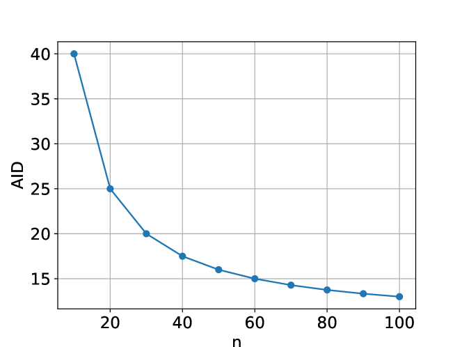
From our observations, one can expect that the more tasks are available, the more drastic the difference between single-task ID and multi-task AID can become. Figure 1 visualizes this phenomenon for the MNIST SP dataset. One can indeed see a clear decrease in the AID with a growing number of available tasks, whereas the single-task ID would not be affected by this.
5 Generalization Guarantees
The result in the previous section suggests that using the representation (2), even quite complex models can be represented with only a quite small number of values. This suggests that the good generalization properties of deep multi-task learning might be explainable by generalization bounds that exploit the representation (3).
Our main theoretical contribution in this work is a demonstration that this is indeed possible: we derive a new generalization bound for multi-task learning that captures the complexity of all models by their joint encoding length. Technically, we provide high probability upper-bounds for the true tasks based on the training error , and properties of the model.
5.1 Background and Related Work
Before we formulate our results, we remind the reader of some core concepts and results from the literature.
Definition 5.1.
For any base set, , we call a function a (prefix-free) encoding, if for all with , the string is a not a prefix of the string . The function , given by we call the encoding length function of .
Prefix-free codes have a number of desirable properties. In particular, they are uniquely and efficiently decodable. Famous examples include variable-length codes, such as Huffman codes (Huffman, 1952) or Elias codes (Elias, 1975), but also the naive encoding that represents each value of a vector with floating-point values by a fixed-length binary string.
Classical results allow deriving generalization guarantees from the encodings of models.
Definition 5.2.
For any model set, , an encoder with a base set is called a model encoder.
Model encodings can be as simple as storing all model parameters in a fixed length (e.g. 32-bit) floating point format. For a -parameter model, the corresponding length function would simply be . Alternatively, storing only the non-zero coefficient values as (index, value) leads to a length function , where is the number of non-zero parameter values. For highly sparse models, this value can be much smaller than the naive encoding. Over the years, many more involved schemes have been introduced, including, e.g., weight quantization (Choi et al., 2020), and entropy or arithmetic coding of parameter values (Frantar & Alistarh, 2024).
Theorem 5.3 (Shalev-Shwartz & Ben-David (2014), Theorem 7.7).
Let be a model encoding scheme with length function . Then, for any , the following inequality holds with probability at least (over the random training data of size ): for all
| (4) |
Theorem 5.3 states that models can be expected to generalize well, i.e., have a smaller difference between their training risk and expected risk, if their encodings are short. Specifically, the dominant term in the complexity term of (4) is . Consequently, for the bound to become non-vacuous (i.e. the right-hand side to be less than 1), in particular, the encoding length must not be much larger than the number of training examples.
5.2 New Guarantees for Multi-Task Learning
We now introduce a generalization of Theorem 5.3 to the multi-task situation. First, we define two types of encoders.
Definition 5.4.
For any model set, , an encoder with base set (e.g. arbitrary length tuples of models) we call a multi-task model encoder.
Multi-task model encoders generalize (single-task) model encoders in the sense of Definition 5.2 by allowing more than one model to be encoded at the same time. By exploiting redundancies between the models, shorter encoding lengths can be achievable. For example, if multiple models share certain parts, such as feature extraction layers, those would only have to be encoded once.
Any such construction will work better (i.e. results shorter length functions) in some situations, but potentially worse in another situation, depending on if and how the tasks to be learned are related. For multi-task learning, it would therefore be beneficial if one could choose the encoding scheme in a data-dependent way. To formalize this, we introduce meta-encoders.
Definition 5.5.
An encoder is called a meta-encoder if its base set is a set of multi-task model encoders.
While meta-encoders are less intuitive objects than, e.g., standard model encoders, they nevertheless serve an important purpose in our analysis, because they allow formalizing the concept of shared versus task-specific information. For example, if all models reside in a low-dimensional subspace of the parameter space, the meta-encoder could encode the subspace, while the multi-task model encoder only encodes the representation of the models within that subspace.
We are now ready to formulate our main results: new generalization bounds for multi-task learning based on the lengths of meta- and multi-task model encoders.
Theorem 5.6.
Let be a set of multi-task model encodings with length functions for . For any meta-encoding with length function , and any , the following inequality holds with probability at least over the sampling of the training data: for all and for all
| (5) | |||
Theorem 5.6 directly generalizes Theorem 5.3 to the multi-task situation.
In addition, we also state an alternative fast-rate bound based on the PAC-Bayes framework.
theoremfastrate In the settings of Theorem 5.6, for any multi-task model encoding, any meta-encoding, and any , the following holds with probability at least over the sampling of the training data:
| (6) | ||||
| where | ||||
| (7) | ||||
is the Kullback–Leibler divergence between Bernoulli distributions with mean and . Fast-rate bounds tend to be harder to prove and interpret, but they offer tighter results when the empirical risk is small. Specifically, the complexity term in Theorem 5.6 scales like when the empirical risk is zero, whereas in Theorem 5.6 the scaling behaviour is always . For a more detailed discussion, see Appendix A.
Discussion.
Theorem 5.6 establishes that the multi-task generalization gap (the difference between empirical risk and expected risk) can be controlled by a term that expresses how compactly the models can be encoded. Because the inequality is uniform with respect to , the multi-task encoding scheme can be chosen in a data-dependent way, where a tighter guarantee follows if the multi-task encoding scheme itself can be compactly represented.
To get a better intuition of this procedure, we consider two special cases. First, assume a naive encoding, where consists of a single element, , which itself is the naive multi-task model encoder that simply stores a -dimensional parameter vector for each model in fixed-width form. Then and , and the resulting complexity term is of the order , as classical VC theory suggests.
In contrast, assume the setting of Section 3, where each task is encoded as a weighted linear combination of dictionary elements, each of which is computed as the product of a large random matrix with an -dimensional parameter vector. Setting to be the set of all such bases, one obtains (for now disregarding potential additional savings by storing coefficients more effectively than with fixed width bits), and . Consequently, the complexity term in Theorem 5.6 become , i.e. the ambient dimension of the previous paragraph is replaced by exactly the amortized intrinsic dimension of Definition 3.1.
| Dataset | MNIST SP | MNIST PL | Folktables | Products | split-CIFAR10 | split-CIFAR100 |
|---|---|---|---|---|---|---|
| Single task [%] | 61.2 | 57.6 | 56.6 | 33.2 | 87.4 | 99.4 |
| MTL (Theorem 5.6) [%] | 23.0 | 40.4 | 39.4 | 22.2 | 52.9 | 86.9 |
| MTL (Theorem 5.6) [%] | 19.6 | 35.0 | 38.8 | 20.3 | 52.7 | 83.0 |
5.3 Proofs
In this section, we provide the proof for Theorem 5.6. The proof of Theorem 5.6 requires more involved tools, so we present it in the appendix.
Proof of Theorem 5.6.
We rely on standard arguments for coding-based generalization bounds, which we adapt to the setting of multiple tasks with potentially different data distributions.
For any , let be the training data available for a task and let be its loss function. For any tuple of models, , we define random variables , where is the number of tasks and is the number of samples per task, such that
| (8) | ||||
| for , and | ||||
| (9) | ||||
Therefore, based on Hoeffding’s inequality over these random variables, we have for any :
| (10) |
Now, assume a fixed . For any meta-encoder, , and any tuple of models, , we define a weight , where is the length function of the meta-encoder and is the length function of the encoder . We instantiate (10) with a value such that , i.e. . Taking a union bound over all tuples and observing that , because of the Kraft-McMillan inequality for prefix codes (Kraft, 1949; McMillan, 1956), we obtain
| (11) | |||
By rearranging the terms, we obtain the claim of Theorem 5.6. ∎
5.4 Computing the Bounds Numerically
In order to apply Theorem 5.6 or Theorem 5.6 in the situation of Section 3, we use a meta-encoder that encodes the coefficient vectors, of the basis representation (2), and a multi-task model encoder that jointly encodes the collection of per-task coefficients, of the per-task representations 3.
The easiest way would be to allow for arbitrary floating point values in the weights and store them in fixed precision, e.g. 32 bit. The resulting lengths functions would be constant: and , such that the dominant part of the complexity term becomes or , respectively. However, it is known that neural networks using quantized weights of fewer bits per parameter can still achieve competitive performance (Han et al., 2016). Therefore, we employ a quantized representation for the parameters we learn, adapting the quantization scheme and learned codebooks of Zhou et al. (2019); Lotfi et al. (2022) to our setting.
Specifically, we use two codebooks, a global one with entries, for quantizing the shared parameters vectors , and a local one with values, for quantizing the per-task parameters vectors .
Now, for any set of models with global , and , the meta-encoder first stores the codebook entries as 16-bit floating-point values. Then, for each entry of the parameter vectors, it computes the index of the codebook entry that represents its value and it stores all indices together using arithmetic coding (Langdon, 1984), which exploits the global statistics of the index values. Analogously, the multi-task model encoder first stores the codebook entries, and then it represents the entries of as indices in the code, and encodes them jointly using arithmetic coding. Note that while the latter process of encoding the model coefficients does not depend on the shared parameters, its decoding process does, because the actual network weights can only be recovered if also the representation basis, , is known.
In practice, training networks with weights restricted to a quantized set is generally harder than training in ordinary floating-point form. Therefore, for our experiments, we follow the procedure from Lotfi et al. (2022). We first train all networks in unconstrained form. We then compute codebooks by (one-dimensional) -means clustering of the occurring weights, and quantizing each weight to the closest cluster center, and then fine-tune the quantized network.
The resulting guarantees then hold for the quantized networks. For Theorem 5.6, we can read off the guarantees on the multi-task risk directly from the explicit complexity term and the training error. For Theorem 5.6, we have to invert the -expression, which however is easily possible numerically. See Appendix A for more details.
5.4.1 Encoding all tasks together
An advantage of our generalization bounds is that they allow us to encode all tasks together. Formally, the bound is based on the term and not . We found this property particularly helpful when using arithmetic coding, as it allows us to achieve a smaller joint encoding length than encoding the task-specific parts separately. Specifically, to encode the indices of relevant codebook entries, we need to encode the length of the codebook, the empirical fraction of occurrences of the indices, and the arithmetic coding given the fractions. For example, when performing multi-task learning on the Folktables dataset, each of the 60 models was characterized as a -dimensional vector (), resulting in 300 task-specific parameters overall. To encode these 300 parameters, we used a codebook with , which required bits for the codebook. bits to encode the empirical fractions, and bits for arithmetic coding. Overall, the encoding length was bits in total, or bits per task. In contrast, encoding the same task-specific models separately would result in the sum of encoding equal to bits or bits per task. This is actually more than double compared to the size of the joint encoding.
5.5 Application to Transfer Learning
The multi-task setting of Section 3 has a straightforward extension to the transfer learning setting. Assume that, after multi-task learning as in previous sections, we are interested in training a model for another related task. Then, a promising approach is to do so in the already-learned representation, given by the learned matrix . In particular, this procedure has a low risk of overfitting, because is low-dimensional and has been constructed without any training data for the new task. In terms of formal guarantees, is a fixed quantity, so no complexity terms appear for it in a generalization bound. However, learning purely in this representation would pose the risk of underfitting, because the MTL representation might not actually be expressive enough also for new tasks.
Consequently, we suggest a transfer learning method with few parameters that combines the flexibility of single-task learning with the advantages of a learned representation. Specifically, for any new task, we learn a model in a subspace of dimensions, of which basis vectors stems from the representation matrix (2), and the remaining come from a random basis as in (1), is a tunable hyperparameter. Formally, the new model has the following representation:
| (12) |
in which is the result of multi-task learning, is a random matrix, and and are learnable parameters for the new task. If the previous tasks are related to the current task, we would expect to have a smaller dimension compared to the case that we do not use .
Theorem 5.3 yields generalization guarantees for this situation, in which only the encoding length of and enters the complexity term, while (like ) do not enter the bound. To encode the coefficients and , we can reuse the codebook of the MTL situation, which is now fixed and therefore does not have to be encoded or learn (and encode) a new one.
Table 3 shows the resulting generalization guarantees. For all datasets, learning a model using the pre-trained representation leads to stronger guarantees than single-task training from scratch. The bounds are always non-vacuous, despite the fact that only a single rather small training set is available in each case.
| Dataset | MNIST SP | MNIST PL | Folktables | Products | CIFAR10 | CIFAR100 |
|---|---|---|---|---|---|---|
| / | 2000 / 10 | 2000 / 10 | 900/ 2 | 2000 / 2 | 453 / 3 | 450 / 10 |
| No transfer [%] | 60.4 | 58.1 | 54.8 | 26.1 | 87.1 | 98.2 |
| Transfer from MTL [%] | 15.1 | 49.7 | 40.1 | 16.1 | 58.0 | 84.8 |
6 Related Work
Multi-task learning (Baxter, 1995; Caruana, 1997) has been an active area of research for many years, first in classical (shallow) machine learning and then also in deep learning, see, e.g., Yu et al. (2024) for a recent survey. Besides practical methods that typically concentrate on the question of how to share information between related tasks (Kang et al., 2011; Sun et al., 2020) and how to establish their relatedness (Juba, 2006; Daumé III & Kumar, 2013; Fifty et al., 2021), there has also been interest from early on to theoretically understand the generalization properties of MTL.
A seminal work in this area is Maurer (2006), where the author studies the feature learning formulation of MTL in which the systems learn a shared representation space and individual per-task classifiers within that representation. In the case of linear features and linear classifiers, he derives a generalization bounds based on Rademacher-complexity. Subsequently, a number of follow-up works extended and refined the results to cover other regularization schemes or complexity measures (Crammer & Mansour, 2012; Pontil & Maurer, 2013; Yousefi et al., 2018; Pentina & Lampert, 2017). However, none of these results are able to provide non-vacuous bounds for overparametrized models, such as deep networks.
A related branch of research targets the problems of representation or meta-learning. There, also multiple tasks are available for training, but the actual problem is to provide generalization guarantees for future learning tasks (Baxter, 2000). A number of works in this area rely on PAC-Bayesian generalization bounds (Pentina & Lampert, 2014; Amit & Meir, 2018; Rothfuss et al., ; Guan & Lu, 2022; Zakerinia et al., 2024), as we do for our Theorem 5.6. This makes them applicable to arbitrary model classes, including deep networks. These results, however, hold only under specific assumptions on the observed tasks, typically that these are themselves i.i.d. sample from a task environment. The complexity terms in their bounds are either not numerically computable, or vacuous by several orders of magnitude for deep networks, because they are computed in the ambient dimensions, not the intrinsic ones. Another difference to our work is that, even those parts of their bound that relate to multi-task generalization are sums of per-task contributions, which prevents the kind of synergetic effects that our joint encoding can provide.
7 Experimental Details
In this section, we provide the details of our experiments. 111Code: https://github.com/hzakerinia/MTL
7.1 Datasets
We use six standard datasets that have occurred in the theoretical multi-task learning literature before.
MNIST Shuffled Pixels (SP): (Amit & Meir, 2018) each task is a random subset of the MNIST (LeCun, 1998) dataset in which 200 of the input pixels are randomly shuffled. The same shuffling is consistent across all samples of that task.
MNIST Permuted Labels (PL): (Amit & Meir, 2018) like MNIST-SP, but instead of shuffling pixels, the label ids of each task are randomly (but consistently) permuted.
Folktables: (Ding et al., 2021) A tabular dataset consisting of public US census information. From personal features, represented in a binary encoding, the model should predict if a person’s income is above or below a threshold. Tasks correspond to different geographic regions.
Multi-task dataset of product reviews (MTPR): (Pentina & Lampert, 2017) The data points are natural language product reviews, represented as vectorial sentence embeddings. The task is to predict if the sentiment of the review is positive or negative. Each product forms a different task.
7.2 Model Architectures
For the image datasets (MNIST-SP, MNIST-PL, split-CIFAR10, and split-CIFAR100) we use convolutional networks. For the MNIST experiments, we use the architecture from Amit & Meir (2018). For the CIFAR experiments, we use the network from Scott et al. (2024). For the vectorial dataset Product and the tabular dataset Folktables, we use 4-layer fully connected networks. For more details about the architectures and optimization procedure, see Appendix B.
The models’ ambient dimensions (number of network weights) range from approximately 12.000 to approximately 120.000, i.e. far more than the available number of samples per task. As random matrices for the single-task parametrization (1), we use the Kronecker product projector of Lotfi et al. (2022), , for . By this construction, the matrix never has to be explicitly instantiated, which makes the memory and computational overhead tractable. For the multi-task representation (3), we use the analogous construction to form .
8 Conclusion
We presented a new parametrization for deep multi-task learning problems that directly allows one to read off its intrinsic dimension. We showed experimentally that for common benchmark tasks, the amortized intrinsic dimension per task can be much smaller than when training the same tasks separately. We derived two new encoding-based generalization bounds for multi-task learning, that result in non-vacuous guarantees on the multi-task risk for several standard benchmarks. To our knowledge, this makes them the first non-vacuous bounds for deep multi-task learning.
A limitation of our analysis in Section 3 is that it relies on a specific representation of the learned models. As such, the values we obtain for the amortized intrinsic dimensionality constitute only upper bounds to the actual, i.e. minimal, number of necessary degrees of freedom. In future work, we plan to explore the option of extending our results also to other popular multi-task parametrization, such as based on prototypes, MAML (Finn et al., 2017), or feature learning (Collobert & Weston, 2008). Note that our theoretical results in Section 5 readily apply to such settings, as long as we define suitable encoders. In this context, as well as in general, it would be interesting to study if our bounds could be improved further by exploiting more advanced techniques for post-training weight quantization (Rastegari et al., 2016; Frantar et al., 2023) or learning models directly in a quantized form (Hubara et al., 2018; Wang et al., 2023).
Impact Statement
This paper presents work whose goal is to advance the field of Machine Learning. There are many potential societal consequences of our work, none which we feel must be specifically highlighted here.
References
- Aghajanyan et al. (2021) Aghajanyan, A., Gupta, S., and Zettlemoyer, L. Intrinsic dimensionality explains the effectiveness of language model fine-tuning. 2021.
- Alquier (2024) Alquier, P. User-friendly introduction to PAC-Bayes bounds. Foundations and Trends in Machine Learning, 17(2):174–303, 2024.
- Amit & Meir (2018) Amit, R. and Meir, R. Meta-learning by adjusting priors based on extended PAC-Bayes theory. In International Conference on Machine Learning (ICML), 2018.
- Ansuini et al. (2019) Ansuini, A., Laio, A., Macke, J. H., and Zoccolan, D. Intrinsic dimension of data representations in deep neural networks. In Conference on Neural Information Processing Systems (NeurIPS), 2019.
- Bartlett & Mendelson (2002) Bartlett, P. L. and Mendelson, S. Rademacher and Gaussian complexities: Risk bounds and structural results. Journal of Machine Learning Research (JMLR), 2002.
- Baxter (1995) Baxter, J. Learning internal representations. In Conference on Computational Learning Theory (COLT), 1995.
- Baxter (2000) Baxter, J. A model of inductive bias learning. Journal of Artificial Intelligence Research (JAIR), 12:149–198, 2000.
- Berend & Tassa (2010) Berend, D. and Tassa, T. Efficient bounds on bell numbers and on moments of sums of random variables. Probability and Mathematical Statistics, 2010.
- Caruana (1997) Caruana, R. Multitask learning. Machine Learning, 28:41–75, 1997.
- Choi et al. (2020) Choi, Y., El-Khamy, M., and Lee, J. Universal deep neural network compression. IEEE Journal of Selected Topics in Signal Processing, 14(4):715–726, 2020.
- Collobert & Weston (2008) Collobert, R. and Weston, J. A unified architecture for natural language processing: Deep neural networks with multitask learning. In International Conference on Machine Learning (ICML), 2008.
- Crammer & Mansour (2012) Crammer, K. and Mansour, Y. Learning multiple tasks using shared hypotheses. In Conference on Neural Information Processing Systems (NeurIPS), 2012.
- Daumé III & Kumar (2013) Daumé III, A. K. H. and Kumar, A. Learning task grouping and overlap in multi-task learning. In International Conference on Machine Learning, pp. 1723–1730, 2013.
- Ding et al. (2021) Ding, F., Hardt, M., Miller, J., and Schmidt, L. Retiring Adult: New datasets for fair machine learning. In Conference on Neural Information Processing Systems (NeurIPS), 2021.
- Dziugaite & Roy (2017) Dziugaite, G. K. and Roy, D. M. Computing nonvacuous generalization bounds for deep (stochastic) neural networks with many more parameters than training data. In Uncertainty in Artificial Intelligence (UAI), 2017.
- Elias (1975) Elias, P. Universal codeword sets and representations of the integers. IEEE Transactions on Information Theory, 21(2):194–203, 1975.
- Fifty et al. (2021) Fifty, C., Amid, E., Zhao, Z., Yu, T., Anil, R., and Finn, C. Efficiently identifying task groupings for multi-task learning. Advances in Neural Information Processing Systems, 34:27503–27516, 2021.
- Finn et al. (2017) Finn, C., Abbeel, P., and Levine, S. Model-agnostic meta-learning for fast adaptation of deep networks. In International Conference on Machine Learning (ICML), 2017.
- Frantar & Alistarh (2024) Frantar, E. and Alistarh, D. QMoE: Practical sub-1-bit compression of trillion-parameter models. In Conference on Machine Learning and Systems (MLSys), 2024.
- Frantar et al. (2023) Frantar, E., Ashkboos, S., Hoefler, T., and Alistarh, D. GPTQ: Accurate post-training quantization for generative pre-trained transformers. In International Conference on Learning Representations (ICLR), 2023.
- Glorot & Bengio (2010) Glorot, X. and Bengio, Y. Understanding the difficulty of training deep feedforward neural networks. In International Conference on Artificial Intelligence and Statistics (AISTATS), 2010.
- Guan & Lu (2022) Guan, J. and Lu, Z. Fast-rate PAC-Bayesian generalization bounds for meta-learning. In International Conference on Machine Learning (ICML), 2022.
- Han et al. (2016) Han, S., Mao, H., and Dally, W. J. Deep compression: Compressing deep neural networks with pruning, trained quantization and huffman coding. In International Conference on Learning Representations (ICLR), 2016.
- Hubara et al. (2018) Hubara, I., Courbariaux, M., Soudry, D., El-Yaniv, R., and Bengio, Y. Quantized neural networks: Training neural networks with low precision weights and activations. Journal of Machine Learning Research (JMLR), 18(187):1–30, 2018.
- Huffman (1952) Huffman, D. A. A method for the construction of minimum-redundancy codes. Proceedings of the IRE, 40(9):1098–1101, 1952.
- Juba (2006) Juba, B. Estimating relatedness via data compression. In International Conference on Machine Learning (ICML), 2006.
- Kang et al. (2011) Kang, Z., Grauman, K., and Sha, F. Learning with whom to share in multi-task feature learning. In Proceedings of the 28th International Conference on Machine Learning (ICML-11), pp. 521–528, 2011.
- Kraft (1949) Kraft, L. G. A device for quantizing, grouping, and coding amplitude-modulated pulses. Master’s thesis, Massachusetts Institute of Technology, 1949.
- Krizhevsky (2009) Krizhevsky, A. Learning multiple layers of features from tiny images. Technical report, University of Toronto, 2009.
- Langdon (1984) Langdon, G. G. An introduction to arithmetic coding. IBM Journal of Research and Development, 28(2):135–149, 1984.
- LeCun (1998) LeCun, Y. The mnist database of handwritten digits. http://yann. lecun. com/exdb/mnist/, 1998.
- Li et al. (2018) Li, C., Farkhoor, H., Liu, R., and Yosinski, J. Measuring the intrinsic dimension of objective landscapes. In International Conference on Learning Representations (ICLR), 2018.
- Lotfi et al. (2022) Lotfi, S., Finzi, M., Kapoor, S., Potapczynski, A., Goldblum, M., and Wilson, A. G. PAC-Bayes compression bounds so tight that they can explain generalization. In Conference on Neural Information Processing Systems (NeurIPS), 2022.
- Lotfi et al. (2024) Lotfi, S., Finzi, M. A., Kuang, Y., Rudner, T. G. J., Goldblum, M., and Wilson, A. G. Unlocking tokens as data points for generalization bounds on larger language models. In Conference on Neural Information Processing Systems (NeurIPS), 2024.
- Maurer (2004) Maurer, A. A note on the PAC Bayesian theorem. arXiv preprint arXiv:cs.LG/0411099, 2004.
- Maurer (2006) Maurer, A. Bounds for linear multi-task learning. Journal of Machine Learning Research (JMLR), 7:117–139, 2006.
- McAllester (1998) McAllester, D. A. Some PAC-Bayesian theorems. In Conference on Computational Learning Theory (COLT), 1998.
- McMillan (1956) McMillan, B. Two inequalities implied by unique decipherability. IRE Transactions on Information Theory, 2(4):115–116, 1956.
- Pentina & Lampert (2014) Pentina, A. and Lampert, C. H. A PAC-Bayesian bound for lifelong learning. In International Conference on Machine Learning (ICML), 2014.
- Pentina & Lampert (2017) Pentina, A. and Lampert, C. H. Multi-task learning with labeled and unlabeled tasks. In International Conference on Machine Learning (ICML), 2017.
- Pontil & Maurer (2013) Pontil, M. and Maurer, A. Excess risk bounds for multitask learning with trace norm regularization. In Conference on Computational Learning Theory (COLT), pp. 55–76. PMLR, 2013.
- Pope et al. (2021) Pope, P., Zhu, C., Abdelkader, A., Goldblum, M., and Goldstein, T. The intrinsic dimension of images and its impact on learning. In International Conference on Learning Representations (ICLR), 2021.
- Rastegari et al. (2016) Rastegari, M., Ordonez, V., Redmon, J., and Farhadi, A. XNOR-net: Imagenet classification using binary convolutional neural networks. In European Conference on Computer Vision (ECCV), 2016.
- (44) Rothfuss, J., Josifoski, M., Fortuin, V., and Krause, A. Scalable PAC-Bayesian meta-learning via the PAC-Optimal hyper-posterior: From theory to practice. Journal of Machine Learning Research (JMLR).
- Scott et al. (2024) Scott, J., Zakerinia, H., and Lampert, C. H. PeFLL: Personalized Federated Learning by Learning to Learn. In International Conference on Learning Representations (ICLR), 2024.
- Seeger (2002) Seeger, M. Pac-bayesian generalisation error bounds for gaussian process classification. Journal of Machine Learning Research (JMLR), 2002.
- Shalev-Shwartz & Ben-David (2014) Shalev-Shwartz, S. and Ben-David, S. Understanding machine learning: From theory to algorithms. Cambridge university press, 2014.
- Sun et al. (2020) Sun, X., Panda, R., Feris, R., and Saenko, K. Adashare: Learning what to share for efficient deep multi-task learning. Advances in Neural Information Processing Systems, 33:8728–8740, 2020.
- Thrun & Pratt (1998) Thrun, S. and Pratt, L. (eds.). Learning to Learn. Kluwer Academic Press, 1998.
- Vapnik & Chervonenkis (1971) Vapnik, V. N. and Chervonenkis, A. Y. On the uniform convergence of relative frequencies of events to their probabilities. Theory of Probability & Its Applications, 16(2):264–280, 1971.
- Wang et al. (2023) Wang, H., Ma, S., Dong, L., Huang, S., Wang, H., Ma, L., Yang, F., Wang, R., Wu, Y., and Wei, F. BitNet: Scaling 1-bit transformers for large language models. arXiv preprint arXiv:2310.11453, 2023.
- Yousefi et al. (2018) Yousefi, N., Lei, Y., Kloft, M., Mollaghasemi, M., and Anagnostopoulos, G. C. Local Rademacher complexity-based learning guarantees for multi-task learning. Journal of Machine Learning Research (JMLR), 19(38):1–47, 2018.
- Yu et al. (2024) Yu, J., Dai, Y., Liu, X., Huang, J., Shen, Y., Zhang, K., Zhou, R., Adhikarla, E., Ye, W., Liu, Y., et al. Unleashing the power of multi-task learning: A comprehensive survey spanning traditional, deep, and pre-trained foundation model eras. arXiv preprint arXiv:2404.18961, 2024.
- Zakerinia et al. (2024) Zakerinia, H., Behjati, A., and Lampert, C. H. More flexible PAC-Bayesian meta-learning by learning learning algorithms. In International Conference on Machine Learning (ICML), 2024.
- Zhao et al. (2018) Zhao, Y., Li, M., Lai, L., Suda, N., Civin, D., and Chandra, V. Federated learning with non-iid data. arXiv preprint arXiv:1806.00582, 2018.
- Zhou et al. (2019) Zhou, W., Veitch, V., Austern, M., Adams, R. P., and Orbanz, P. Non-vacuous generalization bounds at the imagenet scale: a PAC-Bayesian compression approach. In International Conference on Learning Representations (ICLR), 2019.
Appendix A Proofs
A.1 Comparison of the Bounds
Theorem 5.6 which in the PAC-Bayes literature is referred to as a fast-rate bound, can be tighter than the bound of the Theorem 5.6. Specifically, up to a different in the -term we can obtain the bound of the Theorem 5.6 by relaxing the bound of the Theorem 5.6. Based on Pinsker’s inequality, we have and therefore
| (13) |
Combining Theorem 5.6 and equation (13) gives that for every with probability at least , we have:
| (14) |
This is really similar to the bound of Theorem 5.6, except for the extra , which is negligible for large or .
Alternatively, instead of using Pinsker’s inequality, we can numerically find a better upper-bound for . Following Seeger (2002); Alquier (2024), we define
| (15) |
Corollary A.1.
With the same setting as Theorem 5.6, with probability at least , we have:
| (16) |
Note that for a fixed , the function is minimized for , and it is a convex increasing function in , when . Therefore, we can find an upper bound for , by binary search in the range , or Newton’s method as in (Dziugaite & Roy, 2017).
As Table 2 shows, the numeric bounds obtained this way can be tighter bound than the upper bound from the Theorem 5.6.
A.2 Proof of Theorem 5.6.
In this section, we provide the proof for Theorem 5.6. Since our hypothesis set is discrete, we use a union-bound approach, similar to the proof of Theorem 5.6. A similar result can be proved using the PAC-Bayes framework and change of measure, similar to the fast-rate bounds in Guan & Lu (2022), but we found our version to be conceptually simpler.
*
Proof.
For any fixed tuple of models, , we have
| (17) | ||||
| (18) |
Subsequently, we follow the steps of the proof of Theorem 5.6. Assume a fixed . For any meta-encoder, , and any tuple of models, , we define a weight , where is the length function of the meta-encoder and is the length function of the encoder . We instantiate (18) with a value such that , i.e. . Therefore, we have with probability at least :
| (19) |
Comparison to the fast-rate bounds of Guan & Lu (2022):
As mentioned earlier, Guan & Lu (2022) proved a fast-rate bound for meta-learning which consists of a multi-task bound and a meta bound. The multi-task bound provided here, shares a similar structure with the bound of Guan & Lu (2022), and a similar approach to upper-bound the MGF (Moment generating function). There are three main differences in how to use the bounds. The first one is that they approximate the upper-bound for the based on a closed-form approximation, which has poorer performance compared to the numerical optimization, and even in the cases where the empirical error is not small, their approximation can be even worse than the bound of the Theorem 5.6). The second difference is that they use Gaussian distributions on the networks that scale with ambient dimensionality, making the bounds vacuous by several orders of magnitude. The more structural difference is that the sum of the task-specific complexity terms appears in their bound. On the other hand, we have a joint complexity term for the task-specific part (which in our case is the length of the multi-task encoding), which as explained in the section 5.4.1, is much smaller than the sum of individual ones.
A.3 Auxiliary Lemmas
Lemma A.2.
(Berend & Tassa, 2010)[Proposition 3.2] Let , be a sequence of independent random variables for which , , and . Let be the binomial random variable with distribution . Then for any convex function we have:
| (21) |
Lemma A.3.
Lemma A.4.
Given the datasets of size . For fixed models, , we have
| (23) |
Proof.
Let be the function , this function is convex. If we define , since s are fixed, and samples are independent, the random variables s are independent. Therefore, , and . Let . Because of Lemma A.2 we have
| (24) | ||||
| or equivalently, | ||||
| (25) | ||||
| Because of Lemma A.3, we have: | ||||
| (26) | ||||
Combining these two inequalities completes the proof. ∎
Appendix B Experimental Details
In this section, we provide experimental details to reproduce the results.
B.1 Model Training Details
As mentioned in the section 7, we use an MLP model for Products and Folktables datasets, and convolutional networks for MNIST and CIFAR datasets. The details of the model architectures are provided in Table 5.
All models are implemented in the PyTorch framework. We train them for 400 epochs with Adam optimizer, weight decay of 0.0005, and learning rate from {0.1, 0.01, 0.001}. The hyperparameter (the dimensionality of the random matrices which build ) is chosen from values in {20, 30, 40, 50, 60, 70, 80, 90, 100, 120, 150, 200, 300, 400, 500, 600, 700, 800, 900, 1000, 1200, 1400, 1600, 1800, 2000, 2500, 3000, 3500, 4000, 5000, 6000, 7000, 8000}. The hyperparameter (the number of basis vectors in ) is chosen from values in {5, 10, 15, 20, 30, 35, 40, 50, 60, 70, 80, 90}.
We train all shared and task-specific parameters jointly. After the training is over, we first quantize the shared parameters, and after fixing them, we quantize each task-specific parameter separately. Quantization training is done with epochs using SGD with a learning rate of . For the codebook size, for the single-task learning, we choose it from {2, 3, 5, 10, 15, 20, 30, 40}. For multi-task we choose the codebook size for shared parameters () from {10, 15, 20, 30} and for encoding the joint task-specific vectors we use codebook size () from {3, 10, 15, 20, 25, 30}. For transfer learning, we use a 1-bit hyperparameter to decide if we want to learn a small new codebook for the new task or transfer the codebook from the multi-task learning stage. For each dataset, the hyperparameters are also encoded and considering in compute the length encoding, since we tune the hyperparameter in a data-dependent way.
| dataset | MNIST SP | MNIST PL | Folktables | Products | split-CIFAR10 | split-CIFAR100 | |
|---|---|---|---|---|---|---|---|
|
Single Task |
[%] | 23.4 | 19.4 | 28.0 | 16.0 | 30.4 | 63.9 |
| codebook size | 10 | 10 | 5 | 5 | 10 | 10 | |
| (average) encoding length | 855.4 | 854.3 | 212.6 | 216.4 | 542.5 | 542.0 | |
|
Multi-task |
[%] | 10.1 | 6.6 | 27.2 | 13.9 | 30.5 | 62.7 |
| codebook sizes / | 10 / 3 | 15 / 10 | 10 / 10 | 10 / 10 | 10 / 20 | 20 / 10 | |
| 2323 | 14887 | 1586 | 1192 | 2358 | 4209 | ||
| 508 | 4796 | 686 | 1128 | 4144 | 3341 | ||
| (average) encoding length | 94.4 | 651.1 | 37.9 | 38.7 | 65.0 | 75.5 | |
| Datasets | Layer | Details |
|---|---|---|
| MNIST-SP/ MNIST-PL | Conv1 | Conv2d(input: , output: , kernel: ) |
| Activation | ELU | |
| Pooling | MaxPool2d(kernel: ) | |
| Conv2 | Conv2d(input: , output: , kernel: ) | |
| Activation | ELU | |
| Pooling | MaxPool2d(kernel: ) | |
| Flatten | - | |
| FC1 | Linear(input: Conv Output, output: ) | |
| FC_out | Linear(input: , output: Output_dim) | |
| split-CIFAR10/ split-CIFAR100 | Conv1 | Conv2d(input: , output: , kernel: ) |
| Activation | ReLU | |
| Pooling | MaxPool2d(kernel: ) | |
| Conv2 | Conv2d(input: , output: , kernel: ) | |
| Activation | ReLU | |
| Pooling | MaxPool2d(kernel: ) | |
| Flatten | - | |
| FC1 | Linear(input: , output: ) | |
| FC2 | Linear(input: , output: ) | |
| FC3 | Linear(input: , output: Output_dim) | |
| Products/ Folktables | FC1 | Linear(input: input_dim, output: ) |
| Activation | ReLU | |
| FC2 | Linear(input: , output: ) | |
| Activation | ReLU | |
| FC3 | Linear(input: , output: ) | |
| Output | Linear(input: , output: Output_dim) |