The tricritical Ising CFT and conformal bootstrap

Abstract

The tricritical Ising CFT is the IR fixed-point of $\lambda\phi^{6}$ theory. It can be seen as a one-parameter family of CFTs connecting between an $\varepsilon$-expansion near the upper critical dimension $3$ and the exactly solved minimal model in $d=2$. We review what is known about the tricritical Ising CFT, and study it with the numerical conformal bootstrap for various dimensions. Using a mixed system with three external operators $\{\phi\sim\sigma,\,\phi^{2}\sim\epsilon,\,\phi^{3}\sim\sigma^{\prime}\}$, we find three-dimensional “bootstrap islands” in $d=2.75$ and $d=2.5$ dimensions consistent with interpolations between the perturbative estimates and the 2d exact values. In $d=2$ and $d=2.25$ the setup is not strong enough to isolate the theory. This paper also contains a survey of the perturbative spectrum and a review of results from the literature.

1 Introduction

It is well-known that the scalar theory with interaction $\mathcal{L}=\frac{1}{2}({\partial}\phi)^{2}+\frac{1}{2}m^{2}\phi^{2}+\frac{1}{24}\lambda\phi^{4}$ has a non-trivial infrared (IR) fixed-point of the renormalisation group (RG), which is attained by tuning the renormalised mass parameter $m^{2}$ to zero. This fixed-point is described by the Ising conformal field theory (CFT) and exists in spacetime dimensions $d$ below the upper critical dimension $4$. In this paper we study instead the action

$$S=\int d^{d}x\left(\frac{1}{2}{\partial}_{\mu}\phi{\partial}^{\mu}\phi+\frac{u_{2}}{2}\phi^{2}+\frac{u_{4}}{4!}\phi^{4}+\frac{\lambda}{6!}\phi^{6}\right).$$ (1)

By tuning both $u_{2}$ and $u_{4}$, this theory flows to an IR fixed-point which describes tricritical behaviour and is denoted the tricritical Ising CFT. The interaction $\phi^{6}$ becomes marginal in the upper critical dimension $d=3$, leading to a perturbative expansion in ${\varepsilon}=3-d$. The Ising and tricritical Ising CFTs are the first instances in a sequence of multicritical fixed-points which are dominated by the interaction $\lambda\phi^{2k}$ and have upper critical dimensions $d_{c}(k)=\frac{2k}{k-1}$. They are believed to be connected to the diagonal minimal models $\mathcal{M}_{k+2,k+1}$ Zamolodchikov:1986db , which are a sequence of exactly solved CFTs in two dimensions Belavin:1984vu ; Friedan:1983xq ; Cappelli:1987xt . Although the picture of a sequence of 2d CFTs connecting to perturbative expansions near the upper critical dimensions is natural from field theory and has been supported by non-perturbative RG studies in fractional spacetime dimensions Codello:2012sc ; Codello:2014yfa ; Hellwig:2015woa , it remains conjectural.

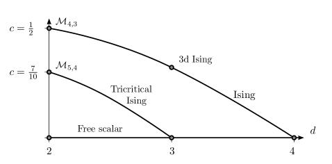
Figure 1: Continuous families of CFTs discussed in this work. The circles represent local unitary theories in integer dimensions. The vertical axis is a proxy for interaction strength, and $c$ is the 2d central charge.

Here we will consider the tricritical Ising CFT from the perspective of the modern conformal bootstrap Rattazzi:2008pe . This programme has led to great success for a variety of theories, see Poland:2018epd ; Rychkov:2023wsd for reviews. To a large extent, the development of the conformal bootstrap has been guided by the following sequence of results for the Ising CFT:

• Single correlator bootstrap produced an exclusion plot in the space spanned by the lowest two scaling dimensions, with a kink at values corresponding to the Ising CFT in $d=2$ Rychkov:2009ij and $d=3$ El-Showk:2012cjh dimensions.

• Using mixed-correlator bootstrap, the kink was converted to an isolated island in parameter space Kos:2014bka . With improved algorithms and numerical strength, the island has been shrunk dramatically to give high-precision data for the 3d Ising CFT Kos:2016ysd ; Chang:2024whx .

• An estimate for the low-lying spectrum can be generated using the extremal functional method ElShowk:2012hu ; El-Showk:2014dwa . This has produced a large set of data for low-lying operators in the Ising CFT Simmons-Duffin:2016wlq .

• Finally, studies for fractional spacetime dimensions $d$ have corroborated the existence of the Ising CFT as a family of CFTs parametrised by $d$ El-Showk:2013nia ; Cappelli:2018vir ; Henriksson:2022gpa ; Bonanno:2022ztf .

In this paper we initiate an attempt to repeat this bootstrap success for the tricritical Ising CFT, and pave the way for future work on related theories, in particular tricritical $O(n)$ models (see discussion in section 5.3). Aware that the 2d theory is exactly solved, our primary goal is to isolate the theory to islands for intermediate, fractional, values of $d$.

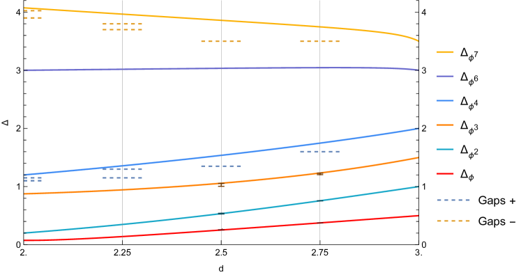
Figure 2: Figure describing our setup and results. The error-bars in $d=2.5$ and $d=2.75$ represent our three-dimensional islands (2)–(3). Solid lines are Padé approximants (20) and the dashed lines are the spectral gaps we assume above the external operators in the ${\mathbb{Z}}_{2}$-even (blue tones) and ${\mathbb{Z}}_{2}$-odd (orange tones) sectors. The islands are almost invisible at this scale, see figure 3 for a log plot of anomalous dimensions. In $d=2$ and $d=2.25$ we do not find islands with the current precision.

Our main results follow from numerical conformal bootstrap of the system of all four-point correlators involving the three lowest-lying scalar operators in the theory: $\{\phi,\phi^{2},\phi^{3}\}$, in 2d denoted $\{\sigma,\epsilon,\sigma^{\prime}\}$. We design a set of gap assumptions to single out this theory from other theories or solutions to crossing – in particular we impose a large gap in the ${\mathbb{Z}}_{2}$-odd sector after $\phi^{3}$, motivated by the fact that $\phi^{5}$ is missing in the spectrum and the next ${\mathbb{Z}}_{2}$-odd operator, perturbatively, is $\phi^{7}$. With this setup, we find bootstrap islands in $d=2.75$ and $d=2.5$ dimensions, with scaling dimensions rigorously confined to the intervals

$$d =2.75: \Delta_{\phi} =0.375405(145), \Delta_{\phi^{2}} =0.75511(121), \Delta_{\phi^{3}} =1.2181(128),$$ (2)

$$d =2.5: \Delta_{\phi} =0.25574(155), \Delta_{\phi^{2}} =0.5344(57), \Delta_{\phi^{3}} =1.029(25),$$ (3)

shown also in figure 2 and 3. These intervals represent the maximal extent along the three coordinate axes of our bootstrap islands. We have not mapped out the precise shape of these islands, instead we used the recent “navigator” approach Reehorst:2021ykw to work out their delimitations. The navigator was also used for locating the islands in parameter space, as illustrated in figure 4.

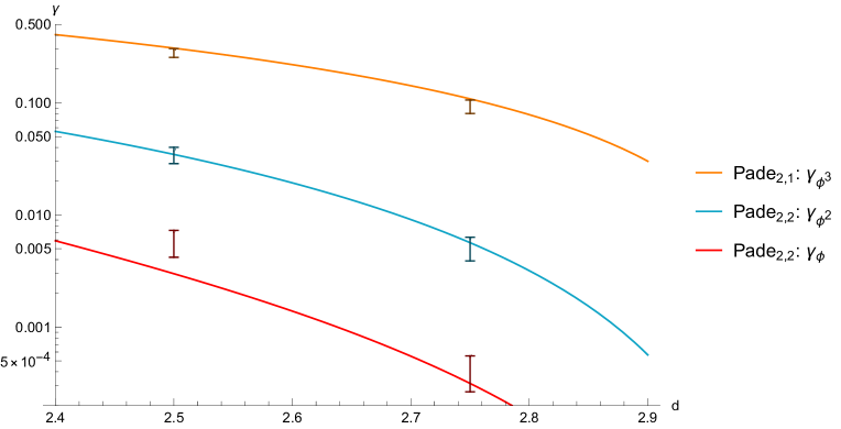
Figure 3: Logarithmic plot of our islands (2)–(3) in terms of anomalous dimensions $\gamma$. The three intervals for a fixed $d$ represent three-dimensional islands (rigorous intervals) and the solid lines are Padé approximants (20).

In $d=2$ and $d=2.25$, our navigator search did not terminate but drifted away, indicating that with the assumptions used and at the present derivative-order ($\Lambda=19$), the numerics is not strong enough to isolate the theory to an island, but rather to a peninsula. This happened even when starting from the exact values in $d=2$: $\Delta_{\phi}=\frac{3}{40}$, $\Delta_{\phi^{2}}=\frac{1}{5}$, $\Delta_{\phi^{3}}=\frac{7}{8}$ and using somewhat stringent gap assumptions. In order to convert these peninsulas to actual islands in $d=2$ and $d=2.25$, we would need to either increase the derivative-order, or consider scanning over more observables/parameters. We discuss the latter in section 4.8.

In the body of the paper, we review the tricritical Ising CFT, discuss strategies and general lessons for the bootstrap, which will pertain to future studies, and present our results. In section 2 we outline the experimental picture, before gathering known results from the literature in the $3-{\varepsilon}$ expansion and in $d=2$. We also present a small collection of new order-${\varepsilon}$ anomalous dimensions computed using the one-loop dilatation operator. In section 3, we give an instrumental view of the bootstrap, emphasising the functionality of recent computational frameworks (specifically we use Simpleboot by Ning Su simpleboot ) which automatise many technical parts of the implementation, allowing the user to focus on the physically meaningful aspects. In section 4 we explain in detail our setup and present all the results. Finally, in section 5 we give an outlook covering several proposed directions. With some minimal prerequisites, the sections 2, 3, 4 and 5 of this paper can be read independently.

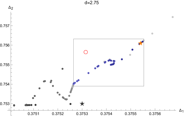
Figure 4: Navigator run in $d=2.75$ projected onto the subspace $(\Delta_{\phi},\Delta_{\phi^{2}})$. Gray is positive navigator values (ruled-out points), purple is negative (allowed points). We display plots including the $\Delta_{\phi^{3}}$ axis in figure 9. The rectangle represents our rigorous bound, found using additional navigator searches along the different axes (appendix A.2), and the red circle the Padé approximant (20). Although the starting point (dark star) is farther away from the allowed points than the Padé approximant, the navigator search still finds the island.

2 The tricritical Ising CFT

In this section, we review various facts about the tricritical Ising CFT. We take a non-perturbative perspective on the theory, viewing a CFT as a set of conformal primary operators with consistent $n$-point correlators. The experimentally measurable critical exponents are related to the scaling dimensions of certain low-lying operators in the spectrum. Within this non-perturbative perspective, the spectrum can be organised by scaling dimension $\Delta$, spin $\ell$, and global-symmetry representation $R$ of the primary operators. Thus, a presentation of the spectrum would be to give for each $(R,\ell)$, a list of all operators with these quantum numbers ordered by increasing scaling dimension.

Apart from the spectrum, the data characterising a CFT also contains the OPE coefficients $\lambda_{ijk}$. Together the spectrum and the set of OPE coefficients completely fix two- and three-point functions of the CFT. Higher-point functions can be determined iteratively by the OPE; for the four-point function it leads to the famous conformal block decomposition

$${\mathcal{G}}_{ijkl}(u,v)=\sum_{{\mathcal{O}}}\lambda_{ij{\mathcal{O}}}\lambda_{kl{\mathcal{O}}}g_{\tau_{\mathcal{O}},\ell_{\mathcal{O}}}(u,v),$$ (4)

where $g_{\tau,\ell}(u,v)$ are the conformal blocks (depending implicitly also on the combinations $\Delta_{i}-\Delta_{j}$ and $\Delta_{k}-\Delta_{l}$), $u,v$ are the conformal cross-ratios, and $\tau=\Delta-\ell$ is the twist.

For the theory studied here, we have access to a perturbative expansion in $d=3-{\varepsilon}$ dimensions, which allows us to connect the non-perturbative perspective with a perturbative construction of operators. With this in mind, we can switch between the non-perturbative notation (first singlet scalar, second singlet scalar etc.) and a perturbative notation ($\phi^{2}$, $\phi^{4}$, etc.).

Near the upper critical dimension, operator dimensions have been computed perturbatively, for instance

$$\Delta_{\phi} =\frac{1}{2}-\frac{{\varepsilon}}{2}+\frac{{\varepsilon}^{2}}{1000}+\left(\frac{2279}{375000}+\frac{27\pi^{2}}{40000}\right){\varepsilon}^{3}+O({\varepsilon}^{4}),$$ (5)

$$\Delta_{\phi^{2}} =1-{\varepsilon}+\frac{4{\varepsilon}^{2}}{125}+\left(\frac{3866}{46875}+\frac{171\pi^{2}}{10000}\right){\varepsilon}^{3}+O({\varepsilon}^{4}),$$ (6)

which are results of a six-loop computation Hager1999 ; Hager:2002uq reviewed below. In two dimensions, the theory is exactly solvable Belavin:1984vu , and scaling dimensions take exact values,

$$\Delta_{\phi}|_{2d} =\frac{3}{40}=0.75\,, \Delta_{\phi^{2}}|_{2d} =\frac{1}{5}=0.2\,, \Delta_{\phi^{3}}|_{2d} =\frac{7}{8}=0.875\,,$$

$$\Delta_{\phi^{4}}|_{2d} =\frac{6}{5}=1.2\,, \Delta_{\phi^{6}}|_{2d} =3\,.$$ (7)

It is expected that resummation of the results $3-{\varepsilon}$-expansion should reproduce these values in $d=2$ with some accuracy, however with the orders available this has not been successful.

2.1 Tricritical physics

The tricritical Ising CFT is physically relevant in the context of systems with ${\mathbb{Z}}_{2}$ symmetry and two relevant symmetry-preserving parameters. In the example below, these parameters are temperature and a chemical potential. There is a two-dimensional phase diagram in these parameters, dividing the parameter space into different phases distinguished by lines of phase transitions. These transitions are either first-order or continuous, and the continuous transitions are generically described by the (normal) Ising CFT. The tricritical Ising CFT appears when several lines of phase transitions meet.

The canonical example is the Blume–Capel model, also known as the Ising model with vacancies Blume:1966zz ; Capel1966 . Here we follow Cardy:1996xt , and define the Hamiltonian of this lattice model as

$$\mathcal{H}=-J\sum_{\langle i,j\rangle}s_{i}s_{j}+\Delta\sum_{i}s_{i}^{2}-h\sum_{i}s_{i},$$ (8)

where $\langle i,j\rangle$ denotes the sum over nearest neighbours. Setting $J=1$, the chemical potential $\Delta$ and the temperature $T=1/\beta$ can be taken as the two relevant parameters. Here we consider $h=0$, however including $h\neq 0$, gives an interesting three-dimensional phase diagram, see e.g. Kaufman1981 ; Cardy:1996xt .

Figure 5: Schematic phase diagram of the Blume–Capel model (8). Along the dashed line, the phase transition is first-order; along the solid line, the phase transition is second-order and described by the Ising CFT. The first- and second-order transitions meet at the tricritical point. Figure adapted from Cardy:1996xt .

Figure 5 shows the expected phase diagram for the Blume–Capel model (8) with $h=0$, displaying an ordered phase and a disordered phase separated by a line of phase transitions. At very low temperature, the transition is first-order, while at higher temperatures the transition is second order and described by the Ising CFT. At some point the two different transitions meet, and the transition there is tricritical, described by the tricritical Ising CFT in $d<3$. At this point, tricritical exponents are defined by the following semi-conventional names

$$y_{h}=d-\Delta_{\phi}=\frac{d+2-\eta}{2},\qquad y_{t}=d-\Delta_{\phi^{2}}=\nu^{-1},\qquad y_{g}=d-\Delta_{\phi^{4}}\,.$$ (9)

The RG flow on different points along the phase transition line is shown in figure 6, parametrised by some variable $\upsilon$. To the left of the tricritical point where the transition is first-order, the theory flows to the gapped phase (trivial CFT). To the right, it flows to the Ising CFT. Exactly at the tricritical point, it flows to the tricritical Ising CFT, which stresses that two parameters need to be tuned to reach this point (one more relevant parameter to reach at the critical line, another less relevant to reach the specific point of the critical line). In the vicinity of the tricritical point, the RG flow is slow and one can expect the tricritical exponents to describe the systems over a range of scales before finally transitioning to Ising/gapped.

Figure 6: RG flow on the phase boundary, parametrised by $\upsilon$. $\mathrm{T}$ represents the tricritical Ising transition. The wavy line near the point $\mathrm{T}$ represents a slowdown in the RG flow near the tricritical point, before ultimately flowing towards the Ising (or gapped on the left).

Other models that also have tricritical fixed-points are the spin-1 Ising model (also known as Blume–Emert–Griffiths model Blume:1971zza ), directly related to the above, and spin-$\frac{1}{2}$ Ising metamagnets Nienhuis1976 ; Landau1981 . Here metamagnets refer to models with sizeable interactions of both nearest-neighbour and next-to-nearest-neighbour type near the tricritical point.

While the tricritical Ising CFT does not exist in $d=3$, tricritical phenomena can still occur, but are then described by the Gaussian fixed point (free theory). Some references mention logarithmic corrections but their status does not appear to be definite Maciolek2004 . Examples of real-world systems with tricritical fixed-points are ${}^{3}\mathrm{He}$–${}^{4}\mathrm{He}$ mixtures Blume:1971zza ; FarahmandBafi2015 (see also Maciolek2004 ), four-component fluid mixtures near room temperature Radyshevskaya1962 ; Lang1975 , and physical metamagnets Fisher1975 ; Fisher1975b (e.g. $\mathrm{FeCl_{2}}$ Shang1980 $\mathrm{Dy_{3}Al_{5}O_{12}}$ Giordano1975 ).

In two dimensions, no experimental determinations of classical tricritical behaviour exists to the best of our knowledge. Quantum-tricritical behaviour (referring to $1+1$ dimensions) was discussed in Ejima:2016nkr ; Maffi:2023tkn . Instead significant effort has gone into studying the lattice models discussed above, especially the Blume–Capel model (8). Contrary to the usual Ising model (recovered as $\Delta\to-\infty$), the Blume–Capel lattice model has not been exactly solved. Simulating it on a lattice the picture of figure 5 has been confirmed and the tricritical temperature and chemical potential have been estimated in around

$$(T_{c},\Delta_{c})\approx(0.608,\,1.966),$$ (10)

for $J=1$. See Kwak2015 for a collection of estimates and references. Tuning to the tricritical point, the (tri)critical exponents can then be estimated and tested against the exact values. Methods to simulate the Blume–Capel model include Monte Carlo RG Landau1981 ; Landau1986 , transfer matrix Beale1986 ; Xavier1998 , and the Wang–Landau method Silva2006 ; Kwak2015 , see also Graham2006 for some formal aspects.

2.2 Review of perturbative results

In this section we summarise the set of perturbative results available in the literature, presenting a picture of the spectrum valid in $d-3-{\varepsilon}$ dimensions. In the limit ${\varepsilon}\to 0$, the spectrum of the tricritical model agrees with that of a free scalar, up to a few exceptions implied by the equations of motion. The scaling dimensions and OPE coefficients are then perturbations from the free-theory values, given in an (asymptotic) series in ${\varepsilon}$:

$$\Delta_{\mathcal{O}}=\Delta_{\mathcal{O}}^{\mathrm{free}}+\gamma_{\mathcal{O}}({\varepsilon}),\qquad\lambda_{ijk}=\lambda_{ijk}^{\mathrm{free}}+\lambda_{ijk}^{(1)}{\varepsilon}+\ldots.$$ (11)

The anomalous dimensions $\gamma_{\mathcal{O}}({\varepsilon})=\gamma_{\mathcal{O}}^{(1)}{\varepsilon}+\gamma_{\mathcal{O}}^{(2)}{\varepsilon}^{2}+\ldots$ can be computed by renormalisation of local operators using Feynman diagrammatic computations. OPE coefficients can, in principle, be computed by constructing perturbatively the precise form of the operators and then computing three-point functions, however this is rarely attempted and results for OPE coefficients are sporadic.

In table 1, we give an overview of the spectrum of the model. Conformal primary operators are constructed from scalar field $\phi$ and partial derivatives ${\partial}_{\mu}$, which must be combined in specific ways to satisfy the primary condition. The free-theory dimension of an operator with $k$ fields and $l$ derivatives is $\Delta_{\mathcal{O}}^{\mathrm{free}}=k\frac{d-2}{2}+l$. It is convenient to organise the spectrum by twist $\tau=\Delta-\ell$ and spin $\ell$, as presented in table 1. At twist $\frac{1}{2}$ (we refer to the values of the twist at $d=3$), there is a single primary operator which is the scalar $\phi$. At higher twists, there are primary operators of unbounded spin, and generically also parity-odd operators.

Among the scalar operators we have pure powers of the field, $\phi^{k}$, and from dimension $6$ and onwards also operators constructed using contracted derivatives. The operator $\phi^{5}$ is missing from the spectrum, since the operator at this level is the equation-of-motion operator ${\partial}^{2}\phi-\lambda\phi^{5}$, which is redundant. Moreover, in table 1 we also indicated the expected identification in the 2d tricritical Ising, following Zamolodchikov:1986db (see also (7.120) of DiFrancesco:1997nk ).

For spinning operators, there are some general patterns at low-lying twists, as indicated in table 1: At $\tau=1$, there is a single operator $\mathcal{J}_{\ell}$ at each even spin. These are conserved in the free theory, but for $\ell>2$ acquire anomalous dimensions (21) at order ${\varepsilon}^{2}$ in the interacting theory. Also at $\tau=\frac{3}{2}$, the leading anomalous dimension is at order ${\varepsilon}^{2}$, but in this case they have not been computed. Starting from $\tau=2$, spinning operators generically acquire $O({\varepsilon})$ anomalous dimensions.

Table 1: Structure of the perturbative spectrum of conformal primary operators, organised by twist $\tau=\Delta-\ell$ (in $d=3$) and spin $\ell$.

Twist	Scalar operators	Spinning operators
$1/2$	$\phi\to\sigma(\frac{3}{40})$. Fundamental field/order parameter. $\gamma_{\phi}$ known to $O({\varepsilon}^{3})$ (5).	No primary operators
$1$	$\phi^{2}\to\epsilon(\frac{1}{5})$. Mass/energy operator. $\gamma_{\phi^{2}}$ known to $O({\varepsilon}^{3})$ (6).	$\mathcal{J}_{\ell}=\phi{\partial}^{\ell}\phi$ at even $\ell$. $\mathcal{J}_{2}^{\mu\nu}=T^{\mu\nu}$. $\gamma_{\ell}$ known to $O({\varepsilon}^{2})$ (21).
$3/2$	$\phi^{3}\to\sigma^{\prime}(\frac{7}{8})$. Subleading order parameter. $\gamma_{\phi^{3}}$ known to $O({\varepsilon}^{2})$ (17).	${\partial}^{\ell}\phi^{3}$. $\Sigma_{i}d_{i}q^{i}=\frac{1}{(1-q^{2})(1-q^{3})}$. $\gamma=O({\varepsilon}^{2})$ unknown.
$2$	$\phi^{4}\to\epsilon^{\prime}(\frac{6}{5})$. Subleading energy operator. $\gamma_{\phi^{4}}$ known to $O({\varepsilon}^{3})$ (14).	${\partial}^{\ell}\phi^{4}$. $\Sigma_{i}d_{i}q^{i}=\frac{1}{(1-q^{2})(1-q^{3})(1-q^{4})}$. One operator per spin has non-zero $\gamma$ at $O({\varepsilon})$ (32).
$5/2$	No primary operator (due to equation of motion)	Generic structure. $\gamma$ at $O({\varepsilon})$ can be determined using one-loop dilatation operator, sec. 2.3.
$3$	$\phi^{6}\to{\varepsilon}^{\prime\prime}(3)$. Irrelevant deformation. $\gamma_{\phi^{6}}$ known to $O({\varepsilon}^{3})$ (14).
$>3$	$\phi^{k}$ operators (16). First primary with derivative $\square^{2}\phi^{4}$ at $\Delta=6$ (35).

In tables 2 and 3 we list all individual operators with $\Delta\leqslant 6$ alongside their anomalous dimensions and OPE coefficients with our external operators $\phi$, $\phi^{2}$ and $\phi^{3}$. The results compiled in these tables are a combination of results extracted from the literature, and some leading-order computations performed in section 2.3 below.

2.2.1 Six-loop renormalisation

In work by Hager and Schäfer Hager1999 ; Hager:2002uq , the theory defined by (1) was renormalised in dimensional regularisation in ${\varepsilon}=3-d$. This completely mimics standard renormalisation of $\phi^{4}$ theories in ${\varepsilon}=4-d$ Kleinert:2001hn , although the Feynman integrals that need to be evaluated differ. While Hager1999 ; Hager:2002uq gave results for the $O(n)$ symmetric generalisation of our theory, we present here the case $n=1$. The renormalisation of the action (1) at six loops gives the following anomalous dimensions at order ${\varepsilon}^{3}$:

$$\gamma_{\phi} =0.001{\varepsilon}^{2}+0.012739{\varepsilon}^{3}+O({\varepsilon}^{4}),$$ (12)

$$\gamma_{\phi^{2}} =0.032{\varepsilon}^{2}+0.25124{\varepsilon}^{3}++O({\varepsilon}^{4}),$$ (13)

$$\gamma_{\phi^{4}} =0.8{\varepsilon}+2.29397{\varepsilon}^{2}-28.05898{\varepsilon}^{3}+O({\varepsilon}^{4}),$$ (14)

$$\gamma_{\phi^{6}} =4{\varepsilon}-13.40598{\varepsilon}^{2}+337.6492{\varepsilon}^{3}+O({\varepsilon}^{4}),$$ (15)

where the total scaling dimension is given by $\Delta_{\phi^{k}}=k\left(\frac{1}{2}-\frac{{\varepsilon}}{2}\right)+\gamma_{\phi^{k}}$. The exact expressions behind the numerical values are given in equations (89)–(92) in the appendix, displaying the dependence on the following numbers: $\pi^{2}$, $\zeta_{3}$, $\pi^{4}$, $\beta_{2}$, $\beta_{4}$, $\ln 2$.

Unfortunately, the computation in Hager1999 ; Hager:2002uq does not include any interaction $\frac{u_{3}}{3!}\phi^{3}$, so we do not have access to any six-loop result for this operator. However, in ODwyer:2007brp , the anomalous dimension $\phi^{k}$ was given on closed form to order ${\varepsilon}^{2}$:

$$\gamma_{\phi^{k}}=\frac{k(k-1)(k-2)}{30}{\varepsilon}-k\!\left(\tfrac{131k^{4}-1010k^{3}+1999k^{2}-1117k-18}{15000}+\tfrac{27(k-5)(k-2)(k-1)}{800}\zeta_{2}\right)\!{\varepsilon}^{2}+O({\varepsilon}^{3}),$$ (16)

where $k\neq 5$. This evaluates to

$$\gamma_{\phi^{3}}=0.2{\varepsilon}+1.073598{\varepsilon}^{2}+O({\varepsilon}^{3}).$$ (17)

for $k=3$.

2.2.2 Padé approximants

Instead of a direct use of the truncated series above, due to their asymptotic nature one typically resorts to resummation methods LeGuillou:1979ixc . Here, with access only to a few orders in the expansion, we make use of the simplest method, namely the Padé approximant, which requires a minimal amount of theory and choices. A Padé approximant is an expression

$$\text{Pad\'{e}}_{m,n}({\varepsilon})=\frac{a_{0}+a_{1}{\varepsilon}+\ldots a_{m}{\varepsilon}^{m}}{1+b_{1}{\varepsilon}+b_{2}{\varepsilon}^{2}+\ldots+b_{n}{\varepsilon}^{n}}.$$ (18)

where the $m+n+1$ constants are fixed by matching with a series expansion to order ${\varepsilon}^{m+n}$. A slight modification, used here, is to construct “Padé approximants tied to 2d,” which means that we use a series expansion to one order less, $O({\varepsilon}^{m+n-1})$, and impose that $\text{Pad\'{e}}_{m,n}(1)$ agrees with the known value at ${\varepsilon}=1$.

Applying this procedure for instance to $\Delta_{\phi}$, we find

$$\text{Pad\'{e}}_{2,2}[\Delta_{\phi}]({\varepsilon})=\frac{\frac{1}{2}-\frac{8579056-34425\pi^{2}}{8898000}{\varepsilon}+\frac{418477-2835\pi^{2}}{889800}{\varepsilon}^{2}}{1-\frac{4130056-34425\pi^{2}}{4449000}{\varepsilon}+\frac{15272+2025\pi^{2}}{1483000}{\varepsilon}^{2}}=\frac{0.5-0.925972{\varepsilon}+0.438859{\varepsilon}^{2}}{1-0.851943{\varepsilon}+0.0237747{\varepsilon}^{2}}.$$ (19)

Indeed its small-${\varepsilon}$ expansion matches (5) and it satisfies $\text{Pad\'{e}}_{2,2}[\Delta_{\phi}](1)=\frac{3}{40}$. In the same way, we construct Padé approximants for $\phi^{k}$, $k\leqslant 7$ using the $O({\varepsilon}^{3})$ results for $k=1,2,4,6$ and $O({\varepsilon}^{2})$ from (16) for $k=3,7$. This gives a list of the following Padé approximants, all tied to 2d:

$$\text{Pad\'{e}}_{2,2}[\Delta_{\phi}],\quad\text{Pad\'{e}}_{2,2}[\Delta_{\phi^{2}}],\quad\text{Pad\'{e}}_{2,1}[\Delta_{\phi^{3}}],\quad\text{Pad\'{e}}_{2,2}[\Delta_{\phi^{4}}],\quad\text{Pad\'{e}}_{1,2}[\Delta_{\phi^{6}}],\quad\text{Pad\'{e}}_{1,2}[\Delta_{\phi^{7}}].$$ (20)

In constructing these, we have made choices for the parameters $m$ and $n$, which are normally chosen to be roughly equal. Sometimes a Padé approximant has spurious poles, for instance the approximant $\text{Pad\'{e}}_{2,2}[\Delta_{\phi^{6}}]({\varepsilon})$ has a pole at $0.120745335$. In this case we discarded the approximant and chose one of a lower order.

Table 2: Even operators with engineering dimension $\leqslant 6$, with leading anomalous dimensions, and OPE coefficients computed from Wick contractions. In parentheses we show the leading ${\varepsilon}$ correction where results are available Codello:2017qek ; Codello:2017hhh .

$\ell$	$\Delta$	${\mathcal{O}}$	$\gamma^{(1)}$	$\lambda_{\phi\phi{\mathcal{O}}}^{2}$	$\lambda_{\phi^{2}\phi^{2}{\mathcal{O}}}^{2}$	$\lambda_{\phi^{3}\phi^{3}{\mathcal{O}}}^{2}$	$\lambda_{\phi\phi^{3}{\mathcal{O}}}^{2}$
$0$	$1$	$\phi^{2}$	$0$	$2$	$8$	$18$	$3$
$0$	$2$	$\phi^{4}$	$\frac{4}{5}$	$(\frac{3{\varepsilon}^{2}}{200})$	$6$	$54$	$4$
$0$	$3$	$\phi^{6}$	$4$	$(\frac{{\varepsilon}^{2}}{500})$	$0$	$20$	$(\frac{27{\varepsilon}^{2}}{40})$
$0$	$4$	$\phi^{8}$	$\frac{56}{5}$	$(\frac{7{\varepsilon}^{4}}{16000})$	$0$	$0$	$0$
$0$	$5$	$\phi^{10}$	$24$	$(\frac{63{\varepsilon}^{4}}{25000000})$	$0$	$0$	$0$
$0$	$6$	$\square^{2}\phi^{4}$	$0$	$0$	$\frac{1}{50}$	$\frac{9}{50}$	$0$
$0$	$6$	$\phi^{12}$	$44$	$0$	$0$	$0$	$0$
$2$	$3$	$T_{\mu\nu}$	$0$	$\frac{3}{32}$	$\frac{3}{8}$	$\frac{27}{32}$	—
$2$	$4$	${\partial}^{2}\phi^{4}$	$\frac{8}{25}$	$0$	$\frac{1}{2}$	$\frac{9}{2}$	$\frac{3}{16}$
$2$	$5$	${\partial}^{2}\phi^{6}$	$\frac{68}{25}$	$0$	$0$	$\frac{81}{32}$	$0$
$2$	$6$	$\square{\partial}^{2}\phi^{4}$	$0$	$0$	$\frac{3}{196}$	$\frac{27}{196}$	$0$
$2$	$6$	${\partial}^{2}\phi^{8}$	$\frac{44}{5}$	$0$	$0$	$0$	$0$
$3$	$5$	${\partial}^{3}\phi^{4}$	$\frac{4}{35}$	—	—	—	$\frac{5}{256}$
$4$	$5$	$\mathcal{J}^{(4)}$	$0$	$\frac{35}{8192}$	$\frac{35}{2048}$	$\frac{315}{8192}$	$0$
$4$	$6$	$({\partial}^{4}\phi^{4})_{a}$	$0$	$0$	$\frac{9}{1120}$	$\frac{81}{1120}$	$0$
$4$	$6$	$({\partial}^{4}\phi^{4})_{b}$	$\frac{4}{15}$	$0$	$\frac{1}{35}$	$\frac{9}{35}$	$\frac{105}{8192}$

2.2.3 Further results from the literature

Here we collect references and additional results for the tricritical Ising CFT in $d=3-{\varepsilon}$ dimensions. Apart from Hager1999 ; Hager:2002uq , classical references for diagrammatic computations are Stephen1973 ; Stephen1975 ; Lewis:1978zz ; Boyanovsky:1979qf ; McKeon:1992cs . For the tricritical $n$-vector model (tricritical $O(n)$ CFT), classical references are Pisarski:1982vz ; Pisarski:1983gn . More recent works on these theories are ODwyer:2007brp ; Basu:2015gpa ; Codello:2017qek ; Codello:2017epp ; Codello:2017hhh ; Sakhi:2021uir .

The leading anomalous dimensions of the twist-1 operators (broken currents) $\mathcal{J}_{\ell}=\phi{\partial}^{\ell}\phi$ were computed in Gliozzi:2017gzh using multiplet-recombination methods (Rychkov:2015naa )

$$\Delta_{\mathcal{J}_{\ell}}=1-{\varepsilon}+\ell+\frac{(\ell^{2}-4){\varepsilon}^{2}}{125(4\ell^{2}-1)}+O({\varepsilon}^{3}).$$ (21)

Together with the results (12)–(14) and (16) above, this represents the complete set of literature values of anomalous dimensions as known to the author.

Table 3: Odd operators with engineering dimension $<6$, with leading anomalous dimensions, and OPE coefficients computed from Wick contractions and/or by decomposing the free-theory correlators. We insert, in parentheses, the order ${\varepsilon}$ correction where available from Codello:2017hhh .

$\ell$	$\Delta$	${\mathcal{O}}$	$\gamma^{(1)}$	$\lambda_{\phi\phi^{2}{\mathcal{O}}}^{2}$	$\lambda_{\phi^{2}\phi^{3}{\mathcal{O}}}^{2}$
$0$	$1/2$	$\phi$	$0$	$2$	$3$
$0$	$3/2$	$\phi^{3}$	$\frac{1}{5}$	$3$	$18$
$0$	$7/2$	$\phi^{7}$	$7$	$0$	$(\frac{1889{\varepsilon}^{2}}{20})$
$0$	$9/2$	$\phi^{9}$	$\frac{84}{5}$	$0$	$0$
$0$	$11/2$	$\phi^{11}$	$33$	$0$	$0$
$2$	$7/2$	${\partial}^{2}\phi^{3}$	$0$	$\frac{3}{20}$	$\frac{9}{10}$
$2$	$9/2$	${\partial}^{2}\phi^{5}$	$\frac{29}{25}$	$0$	$\frac{27}{28}$
$2$	$11/2$	${\partial}^{2}\phi^{7}$	$\frac{26}{5}$	$0$	$0$
$3$	$9/2$	${\partial}^{3}\phi^{3}$	$0$	$\frac{5}{616}$	$\frac{15}{308}$
$3$	$11/2$	${\partial}^{3}\phi^{5}$	$\frac{5}{7}$	$0$	$\frac{5}{312}$
$4$	$11/2$	${\partial}^{4}\phi^{3}$	$0$	$\frac{7}{832}$	$\frac{21}{416}$

OPE coefficients in the free theory (${\varepsilon}=0$) can be computed using Wick contractions. For scalar operators $\phi^{k}$, a combinatorial exercise gives

$$\lambda_{\phi^{i}\phi^{j}\phi^{k}}=\frac{\sqrt{i!j!k!}}{\left(\frac{1}{2}(i+j-k)\right)!\left(\frac{1}{2}(i-j+k)\right)!\left(\frac{1}{2}(-i+j+k)\right)!}.$$ (22)

For more complicated operators, the Wick contraction method requires knowing the precise form of the operators, and we delay this discussion to section 2.3 below. For corrections to the OPE coefficients beyond the free theory, only sporadic results are available. We reproduce the following results from Codello:2017qek

$$\lambda_{\phi\phi\phi^{4}}^{2} =\frac{3{\varepsilon}^{2}}{200}, \lambda_{\phi\phi\phi^{6}}^{2} =\frac{{\varepsilon}^{2}}{500}, \lambda_{\phi\phi^{3}\phi^{6}}^{2} =\frac{27{\varepsilon}^{2}}{40}$$

$$\lambda_{\phi\phi\phi^{8}}^{2} =\frac{7{\varepsilon}^{4}}{16000}, \lambda_{\phi\phi\phi^{10}}^{2} =\frac{63{\varepsilon}^{4}}{25000000},$$ (23)

and from Codello:2017hhh

$$\lambda_{\phi\phi^{3}\phi^{4}}^{2} =4-\frac{24{\varepsilon}}{5}, \lambda_{\phi^{2}\phi^{4}\phi^{4}}^{2} =32-\frac{12}{5}\left(32+3\pi^{2}\right){\varepsilon}, \lambda_{\phi^{2}\phi^{2}\phi^{6}}^{2} =\frac{256{\varepsilon}^{2}}{125}, \lambda_{\phi^{2}\phi^{3}\phi^{7}}^{2} =\frac{189{\varepsilon}^{2}}{20}.$$ (24)

The last of these expressions forms part of a tower of OPE coefficients $\lambda_{\phi^{2}\phi^{k}\phi^{k+4}}$, $k=3,4,\ldots$ given in Codello:2017hhh . In writing (23)–(24) we converted the results of Codello:2017qek ; Codello:2017hhh to the CFT conventions with unit-normalised position-space two-point functions. In section 6.3 of Henriksson:2020jwk , the OPE coefficients of the broken currents $\phi{\partial}^{\ell}\phi$ in the $\phi\times\phi$ OPE were computed to order ${\varepsilon}^{2}$, we print these in (93) in appendix B.1. The case $\ell=2$ gives the following result for the central charge

$$\frac{C_{T}}{C_{T,\mathrm{free}}}=1-\frac{4{\varepsilon}^{2}}{1875}+O({\varepsilon}^{3}),$$ (25)

where $C_{T,\mathrm{free}}=\frac{d}{d-1}$ in our conventions.

An alternative way to obtain some OPE coefficients in the free theory is to perform the conformal block decomposition of free-theory correlators, which can be computed using Wick contractions for the external field. The computation is standard, where the most difficult step is the conformal blocks in three dimensions for unequal external operators. These blocks can for instance be computed using the subcollinear expansion explained in appendix A of Bertucci:2022ptt , or by the radial expansion Kos:2013tga ; Hogervorst:2013sma . As a simple example, we find

$${\mathcal{G}}_{\phi^{2}\phi^{2}\phi^{2}\phi^{2}}(u,v) =1+u+\frac{u}{v}+4\sqrt{u}+\frac{4u}{\sqrt{v}}+\frac{4\sqrt{u}}{\sqrt{v}}=1+8g_{1,0}+\frac{3}{8}g_{1,2}+\frac{35}{2048}g_{1,4}$$

$$\quad+\frac{231}{262144}g_{1,6}+\ldots+6g_{2,0}+\frac{1}{2}g_{2,2}+\frac{41}{1120}g_{2,4}+\ldots,$$ (26)

where $g_{\tau,\ell}$ represent the conformal blocks of operators with dimension $\Delta=\tau+\ell$ and spin $\ell$. For non-degenerate operators, the OPE coefficients $\lambda_{\phi^{2}\phi^{2}{\mathcal{O}}}^{2}$ can now be read off – compare (26) with table 2. A case with degeneracy is $(\tau,\ell)=(2,4)$, where we can check that the individual OPE coefficients for ${\mathcal{O}}_{a}$ and ${\mathcal{O}}_{b}$ computed in (37)–(38) below sum up to $\frac{41}{1120}$.

2.3 New perturbative results from one-loop dilatation operator

In this section we are concerned with anomalous dimensions of arbitrary composite operators. In principle these can be computed systematically to any loop order using diagrams, however we are not aware of any such systematic computation in $3-{\varepsilon}$ dimensions. Leaving multiloop results to future work, we use here a convenient method to derive leading-order results, which makes use of conformal perturbation theory Cardy:1996xt , section 5.2, see also Komargodski:2016auf ; Amoretti:2017aze .

Consider a UV CFT perturbed by an operator $\alpha{\mathcal{O}}_{\mathrm{int}}$ such that there is an IR fixed-point at $\alpha=\alpha_{*}\ll 1$. Then the leading correction to the anomalous dimension matrix $\tensor\Gamma{{}_{i}^{j}}$ is proportional to the OPE coefficient $\tensor\lambda{{}_{i{\mathcal{O}}_{\mathrm{int}}}^{j}}$, where the index is raised with the two-point function. Here the UV CFT is the free theory, the IR CFT the tricritical Ising CFT, the interaction is ${\mathcal{O}}_{\mathrm{int}}=\phi^{6}$ and we have $\alpha\sim\lambda\sim{\varepsilon}$. Taking combinatorial and kinematic factors into account, we find the formula,

$$\tensor\Gamma{{}_{i}^{j}}=\frac{{\varepsilon}}{\sqrt{500}}\tensor\lambda{{}_{i\,\phi^{6}}^{j}}.$$ (27)

As a direct example, for the operator $\phi^{k}$, this formula together with (22) gives the expression $\gamma_{\phi^{k}}=\frac{k(k-1)(k-2){\varepsilon}}{30}$, in agreement with the leading term in (16).

For more complicated operators, using (27) requires a few steps, similar to section 4.2 of Henriksson:2022rnm : 1) write a basis of operators with a given scaling dimension and spin, 2) compute the set of OPE coefficients $\tensor\lambda{{}_{i\,\phi^{6}}^{j}}$ involving these operators, 3) diagonalise the anomalous dimension matrix, and 4) identify primary operators among the eigenvectors. For the second step rather than using direct Wick contractions, it is convenient to use the implementation from Hogervorst:2015akt ; Hogervorst:2015tka , which directly gives $\tensor\lambda{{}_{i\,{\mathcal{O}}_{\mathrm{int}}}^{j}}$ with the $j$ index raised, implying that the basis elements chosen in the first step do not need to be unit-normalised.

We give one example, dimension-$6$ operators of spin 4 with four fields. We take as basis,

$${\mathcal{O}}_{1} =\phi^{3}(\alpha.{\partial})^{4}\phi\,, {\mathcal{O}}_{2} =\phi^{2}(\alpha.{\partial})\phi(\alpha.{\partial})^{3}\phi\,, {\mathcal{O}}_{3} =\phi[(\alpha.{\partial})\phi]^{2}(\alpha.{\partial})^{2}\phi\,,$$

$${\mathcal{O}}_{4} =\phi^{2}[(\alpha.{\partial})^{2}\phi]^{2}, {\mathcal{O}}_{5} =[(\alpha.{\partial})\phi]^{4},$$ (28)

where $\alpha.{\partial}=\alpha^{\mu}{\partial}_{\mu}$ for an ancillary null vector $\alpha$, $\alpha^{2}=0$. Evaluating the OPE coefficients using the method of Hogervorst:2015akt ; Hogervorst:2015tka , we find the anomalous dimension matrix

$$\Gamma=\frac{1}{525}{\small\begin{pmatrix}210&840&1260&630&0\\ 10&230&390&60&90\\ 1&26&162&27&36\\ 6&48&324&162&0\\ 0&12&72&0&24\end{pmatrix}},$$ (29)

suppressing ${\varepsilon}$. The eigenvalues are $\left\{0,\frac{4}{35},\frac{4}{15},\frac{8}{25},\frac{4}{5}\right\}$, and include both primaries and descendants. Either by considering the primary condition (operator annihilated by special conformal transformation), or by identifying the eigenvalues $\left\{\frac{4}{5},\frac{8}{25},\frac{4}{35}\right\}$ as anomalous dimensions of primaries at lower spin ($\ell=0,2,3$), we find two new primary operators (left eigenvectors of (29)):

$$\gamma =0: {\mathcal{O}}_{a}\propto-6{\mathcal{O}}_{3}+{\mathcal{O}}_{4}+9{\mathcal{O}}_{5},$$ (30)

$$\gamma =\frac{4}{15}: {\mathcal{O}}_{b}\propto-{\mathcal{O}}_{1}+28{\mathcal{O}}_{2}-12{\mathcal{O}}_{3}-33{\mathcal{O}}_{4}+18{\mathcal{O}}_{5}.$$ (31)

Performing this computation at a number of spins, we discover a structure in the $O({\varepsilon})$ spectrum of $\phi^{4}$-type operators: Exactly one operator at each spin has a non-vanishing anomalous dimension at order ${\varepsilon}$, which takes the following values:

$$\gamma^{(1)}_{\neq 0}=\frac{1}{5}+\frac{3(-1)^{\ell}}{10(\ell+\frac{1}{2})},\qquad\ell=0,2,3,4,5,\ldots.$$ (32)

The first instances are $\frac{4}{5},\frac{8}{25},\frac{4}{35},\frac{4}{15},\frac{8}{55},\frac{16}{65},\frac{4}{25},\frac{4}{17},\frac{16}{95}$. In addition to those, we find operators with $\gamma^{(1)}=0$ existing at spins $4,6,7,\ldots$. The total number of operators at spin $\ell$ is given by the generating function shown in table 1. From twist $\frac{5}{2}$ with five fields and onwards, one arrives at a generic picture, where several operators have non-vanishing $\gamma^{(1)}$, similar to the picture from twist $4$ onwards in $\phi^{4}$ theory.

By executing the computations above, we also discover a collection of towers of operators with fixed number of derivatives but increasing number of fields, directly analogous to Kehrein:1994ff . For these towers, the anomalous dimensions are given by expressions in closed form in $k$, valid for some $k\geqslant k_{0}$, where $k_{0}\leqslant l$ and $l$ is the number of partial derivatives used to construct the operators. We report the following towers:

• The operators $\phi^{k}$, with $\gamma$ given by (16).

• Operators of the form ${\partial}^{2}\phi^{k}$:

  $$\gamma^{(1)}=\frac{(k-3)(k-2)(5k+4)}{150},\qquad k=2,3,4,5,6,\ldots.$$ (33)

  The first few cases are $0,0,\frac{8}{25},\frac{29}{25},\frac{68}{25},\frac{26}{5},\frac{44}{5},\frac{343}{25}$.

• Operators of the form ${\partial}^{3}\phi^{k}$:

  $$\gamma^{(1)}=\frac{(k-3)(7k^{2}-12k-40)}{210},\qquad k=3,4,6,\ldots.$$ (34)

  The first few cases are $0,\frac{4}{35},\frac{5}{7},\frac{146}{35},\frac{52}{7},\frac{419}{35}$. The case $k=5$ ($\gamma=2$) is excluded from the primary spectrum due to equations of motion.

• Operators of the form $\square^{2}\phi^{k}$:

  $$\gamma^{(1)}=\frac{(k-4)(k-2)(5k+3)}{150},\qquad k=4,5,6,\ldots.$$ (35)

  The first few cases are $0,\frac{14}{25},\frac{44}{25},\frac{19}{5},\frac{172}{25},\frac{56}{5}$

• Two operators of the form ${\partial}^{4}\phi^{k}$, with anomalous dimensions

  $$\gamma^{(1)}=\frac{35k^{3}-182k^{2}+32k+684\pm\sqrt{49k^{4}+812k^{3}+37228k^{2}-287184k+508176}}{1050}.$$ (36)

  These exist for $k=2,3,4,5,\ldots$ (upper sign), and for $k=4,5,\ldots$ (lower sign) respectively.

For all of these towers, the largest power of $k$ is always $k^{3}/30$.

The diagonalisation of the anomalous dimension matrix gives not only the eigenvalues, but also the leading form of the eigenvectors. They can then be used to compute unit-normalised OPE coefficients by Wick contractions. For instance, for the operators (30)–(31), we find

$$\lambda_{\phi^{2}\phi^{2}{\mathcal{O}}_{a}} =\frac{3}{\sqrt{1120}}\,, \lambda_{\phi^{3}\phi^{3}{\mathcal{O}}_{a}} =\frac{9}{\sqrt{1120}}\,, \lambda_{\phi\phi^{3}{\mathcal{O}}_{a}} =0\,,$$ (37)

$$\lambda_{\phi^{2}\phi^{2}{\mathcal{O}}_{b}} =\frac{1}{\sqrt{35}}\,, \lambda_{\phi^{3}\phi^{3}{\mathcal{O}}_{b}} =\frac{3}{\sqrt{35}}\,, \lambda_{\phi\phi^{3}{\mathcal{O}}_{b}} =\frac{\sqrt{210}}{128}\,,$$ (38)

as reported in table 2.

2.4 Two-dimensional minimal model

We now review the case $d=2$, where the tricritical CFT becomes the two-dimensional minimal model $\mathcal{M}_{5,4}$. The material here is standard and can for instance be found in DiFrancesco:1997nk ; important original references are Zamolodchikov:1986db ; Lassig:1990xy . The 2d tricritical Ising model has various interesting properties, such as Kramers–Wanniers duality and integrable RG flows, see Lassig:1990xy ; Delfino:1995zk ; Frohlich:2006ch and Zamolodchikov:1987ti ; Zamolodchikov:1991vx ; Zamolodchikov:1991vh ; Fendley:1993xa for some references. Here we focus on aspects related to the spectrum, OPE, and four-point correlators.

In a two-dimensional CFT, the equivalent of conformal primaries are called quasi-primaries, and belong to Virasoro multiplets. In a minimal model, there is a finite number of multiplets, each consisting of a Virasoro primary and an infinite number of Virasoro descendants. The Virasoro primaries are organised in a Kac table, e.g. table 4. In this table, we have identified three sets of names for the Virasoro primaries: Kac labels $\phi_{p,q}$; conventional names $\mathbb{I}$ (identity), $\sigma$ (${\mathbb{Z}}_{2}$-odd) and $\epsilon$ (${\mathbb{Z}}_{2}$-even), where primes denote subleading operators in the respective global symmetry irrep, and the identification with the $3-{\varepsilon}$ expansion through the names $\phi^{k}$.

Table 4: Kac table showing the Virasoro primaries in the minimal model. Based on (7.120) of DiFrancesco:1997nk .

$\phi_{3,1}=\epsilon^{\prime\prime}(3)\sim\phi^{6}$	$\phi_{3,2}=\epsilon^{\prime}(\frac{6}{5})\sim\phi^{4}$	$\phi_{3,3}=\epsilon(\frac{1}{5})\sim\phi^{2}$	$\phi_{3,4}=\mathbb{I}(0)\sim{\mathds{1}}$
$\phi_{2,1}=\sigma^{\prime}(\frac{7}{8})\sim\phi^{3}$	$\phi_{2,2}=\sigma(\frac{3}{40})\sim\phi$	$\phi_{2,3}=\sigma(\frac{3}{40})\sim\phi$	$\phi_{2,4}=\sigma^{\prime}(\frac{7}{8})\sim\phi^{3}$
$\phi_{1,1}=\mathbb{I}(0)\sim{\mathds{1}}$	$\phi_{1,2}=\epsilon(\frac{1}{5})\sim\phi^{2}$	$\phi_{1,3}=\epsilon^{\prime}(\frac{6}{5})\sim\phi^{4}$	$\phi_{1,4}=\epsilon^{\prime\prime}(3)\sim\phi^{6}$

Among the Virasoro primaries, there are restrictions on which operators have non-zero OPE coefficients, determined by fusion rules:

$$\sigma\times\sigma =\mathbb{I}+\epsilon+\epsilon^{\prime}+\epsilon^{\prime\prime}, \sigma\times\epsilon =\sigma+\sigma^{\prime}, \epsilon\times\epsilon =\mathbb{I}+\epsilon^{\prime},\quad\text{etc.}$$ (39)

These lead to additional conditions not imposed by ${\mathbb{Z}}_{2}$ symmetry, for instance, $\lambda_{\epsilon\epsilon\epsilon}=0$, which are not expected to be valid at generic $d>2$ (for instance, in the free 3d theory we have $\lambda^{2}_{\phi^{2}\phi^{2}\phi^{2}}=8$). The complete set of fusion rules with OPE coefficients is

$$\sigma\times\sigma =\mathbb{I}+A\epsilon+\frac{A}{6}\epsilon^{\prime}+\frac{1}{56}\epsilon^{\prime\prime}, \sigma\times\epsilon =A\sigma+\frac{1}{2}\sigma^{\prime}, \sigma^{\prime}\times\sigma =\frac{1}{2}\epsilon+\frac{3}{4}\epsilon^{\prime},$$

$$\sigma^{\prime}\times\epsilon =\frac{1}{2}\sigma\,, \sigma^{\prime}\times\sigma^{\prime} =\mathbb{I}+\frac{7}{8}\epsilon^{\prime\prime}, \epsilon\times\epsilon =\mathbb{I}+\frac{2A}{3}\epsilon^{\prime},$$

$$\sigma\times\epsilon^{\prime} =\frac{A}{6}\sigma+\frac{3}{4}\sigma^{\prime}, \epsilon\times\epsilon^{\prime} =\frac{2A}{3}\epsilon+\frac{3}{7}\epsilon^{\prime\prime}, \sigma^{\prime}\times\epsilon^{\prime} =\frac{3}{4}\sigma\,,$$

$$\epsilon^{\prime}\times\epsilon^{\prime} =\mathbb{I}+\frac{2A}{3}\epsilon^{\prime}, \sigma\times\epsilon^{\prime\prime} =\frac{1}{56}\sigma\,, \epsilon\times\epsilon^{\prime\prime} =\frac{3}{7}\epsilon^{\prime},$$

$$\sigma^{\prime}\times\epsilon^{\prime\prime} =\frac{7}{8}\sigma^{\prime}, \epsilon^{\prime}\times\epsilon^{\prime\prime} =\frac{3}{7}\epsilon\,, \epsilon^{\prime\prime}\times\epsilon^{\prime\prime} =\mathbb{I},$$ (40)

where

$$A=\sqrt{\frac{\Gamma(4/5)\Gamma(2/5)^{3}}{\Gamma(1/5)\Gamma(3/5)^{3}}}=0.915453111397\ldots.$$ (41)

We (re)computed the OPE coefficients using formula (A.5) from Poghossian:2013fda , taken from Poghossian:1989plv and valid for the choice of Kac labels compatible with (A.3) in the same paper, however original references are Dotsenko:1984ad ; Dotsenko:1985hi .

The torus partition function takes the well-known form of a diagonal modular invariant of a minimal model CFT:

$$Z_{m,n}=\sum_{r,s}\chi_{r,s}(\tau)\overline{\chi_{r,s}(\tau)}.$$ (42)

where $\chi_{r,s}$ are the characters of the minimal models. For the tri-critical minimal model (and periodic boundary conditions), the diagonal is the only modular invariant, and the sum is over the states of table 4. For higher minimal models, there are additional modular invariants. In appendix C, we give more details in the partition function (42) and discuss the decomposition in quasiprimaries.

Using Virasoro conformal blocks, one can write down four-point correlation functions of Virasoro primaries. For instance the four-point function of $\sigma\sim\phi\sim\phi_{2,2}$ is given by

$${\mathcal{G}}_{\sigma\sigma\sigma\sigma}^{2d}(z,\bar{z}) =\left|\mathscr{F}_{{\mathds{1}}}(z)\right|^{2}+\lambda_{\sigma\sigma\epsilon}^{2}\left|\mathscr{F}_{\phi_{3,3}}(z)\right|^{2}+\lambda_{\sigma\sigma\epsilon^{\prime}}^{2}\left|\mathscr{F}_{\phi_{1,3}}(z)\right|^{2}+\lambda_{\sigma\sigma\epsilon^{\prime\prime}}^{2}\left|\mathscr{F}_{\phi_{3,1}}(z)\right|^{2},$$ (43)

where $\mathscr{F}_{\phi_{p,q}}(z)$ are Virasoro conformal blocks for four $\phi_{2,2}$ operators, see appendix D.3. The OPE coefficients entering are

$$\lambda_{\sigma\sigma\epsilon}^{2}=A^{2},\qquad\lambda_{\sigma\sigma\epsilon^{\prime}}^{2}=\frac{A^{2}}{36},\qquad\lambda_{\sigma\sigma\epsilon^{\prime\prime}}^{2}=\frac{1}{3136},$$ (44)

as read off from (40). Other correlators are constructed in similar ways; for instance an explicit expression for ${\mathcal{G}}_{\epsilon\epsilon\epsilon\epsilon}(z,\bar{z})$ was given in Friedan:1984rv ; Behan:2017rca and likewise for ${\mathcal{G}}_{\sigma^{\prime}\sigma^{\prime}\sigma^{\prime}\sigma^{\prime}}(z,\bar{z})$ in Maloney:2016kee .

Finally we note that there is a close relation between the tricritical Ising CFT and the first supersymmetric minimal model Friedan:1983xq ; Friedan:1984rv ; Qiu:1986if , where the supersymmetric model is obtained by a Jordan–Wigner transform, see e.g. Hsieh:2020uwb for a recent treatment. Concrete realisations of this model were discussed in Grover:2013rc ; Rahmani:2015qpa .

2.5 Continuation in $\bm{d}$

Finally, we would like to comment on the fact that a fundamental assumption in this paper is that there is a way to continue the tricritical Ising CFT across spacetime dimensions in a consistent way. We do not know of any rigorous treatment of this, but it seems likely that such continuation can be made well-defined. Here we outline a scenario for how this could be formalised, capturing also continuation in group parameters.

We postulate the existence of a family of consistent, but non-local and non-unitary, theories which exist across continuous values of $d$, $\mathcal{CFT}_{d}$. They contain evanescent operators (operators which vanish identically at some integer dimensions due to trace relations Buras:1989xd ; Dugan:1990df ; Hogervorst:2015akt ), and may be defined in the sense of Deligne categories following Binder:2019zqc . At some integer dimensions $d=D\in{\mathbb{Z}}$, we postulate then that there are two theories live on top of each other: One is the specification to $d=D$ of the continuous family: $\mathcal{CFT}_{D}$. The other is the actual local and (often) unitary theory $\texttt{CFT}_{D}$. The latter is a subsector of the former:

$$\texttt{CFT}_{D}\subset\mathcal{CFT}_{D}\,,$$ (45)

in the sense that whenever the same observable exist in both theories, they agree. Since the OPE is closed within operators in $\texttt{CFT}_{D}$, it means that as $d\to D$, a subset of operators in $\mathcal{CFT}_{d}$ forms a closed subsector under the OPE, isomorphic to $\texttt{CFT}_{d}$.

The same idea would hold for continuation in $n$ where $n$ is a group-theory parameter. The work Binder:2019zqc lists for which symmetry groups this is possible. We mention some examples where such continuation has been discussed in detail:

• 2d $O(n)$ models Grans-Samuelsson:2021uor ; Jacobsen:2022nxs . $\mathcal{CFT}_{n}$ is defined as a loop gas model for $n\in[-2,2]$. For $n=1$, the theory $\mathcal{CFT}_{1}$ is still a loop model and has observables like the fractal dimension $d_{f}=\Delta_{T}$, where $\Delta_{T}$ is the dimension of the leading operator in the (continued) rank-2 traceless-symmetric representation. On the other hand $\texttt{CFT}_{1}$ is the 2d Ising CFT, in which $d_{f}$ is not an observable. The limit $n\to 0$ is also interesting, since there $\mathcal{CFT}_{n}$ becomes a logarithmic CFT Cardy:1999zp ; Cardy:2013rqg ; Movahed:2004nr ; Hogervorst:2016itc .

• One can also consider $d$-dimensional critical $O(n)$ loop models, and simultaneously continue in both $n$ and $d$ Shimada:2015gda . The 3d critical $O(n)$ loop model are amendable for simulations, including the case at non-integer values of $n$ Liu:2012ca .

• Similar to 2d $O(n)$ models are $q$-state Potts models, where the group is the symmetric group $S_{q}$ which admits a continuation in $q$ Nivesvivat:2022qvw ; Jacobsen:2022nxs .

We remark that the limit $d\to 2$ is expected to be rather special with respect to the outlined story, since the conformal algebra needs is enhanced to the Virasoro algebra. This imposes an infinite number of constraints that can only be achieved by a drastic reorganisation of the spectrum, in particular at large spin. For Ising, the situation was studied numerically in Cappelli:2018vir , and analytically in Li:2021uki , however more work is needed to clarify the picture.

For the bootstrap, there is also the complication that the theory is non-unitary away from integer dimensions, as pointed out in Hogervorst:2015akt . However, several bootstrap studies have been successfully completed in non-integer dimensions: El-Showk:2013nia ; Cappelli:2018vir ; Henriksson:2022gpa ; Bonanno:2022ztf for Ising, and Sirois:2022vth ; Chester:2022hzt ; Reehorst:2024vyq ; Nakayama:2024iiw for other theories. In these works, the non-unitarity does not seem to cause any problem, most likely because the unitarity-violating operators are high up in the spectrum and/or couple weakly to the external operators.

3 The bootstrap approach

In this section we give an overview of the numerical conformal bootstrap approach. The content is relatively standard by now, as reviewed in Poland:2018epd ; Chester:2019wfx ; PerimeterCourse ; Rychkov:2023wsd . The purpose of this section is to complement these reviews by emphasising the various options available when designing bootstrap algorithms with a specific problem in mind.

3.1 Standard formulation

Consider a set $\mathscr{E}$ of external operators. The starting point of the bootstrap is a set of crossing equations

$$\left\{0=\sum_{\mathcal{O}\in i\times j\,\cap\,k\times l}\lambda_{ij{\mathcal{O}}}\lambda_{kl{\mathcal{O}}}g^{ijkl}_{\Delta_{\mathcal{O}},\ell_{\mathcal{O}}}(u,v)-\sum_{\mathcal{O}\in i\times l\,\cap\,k\times j}\lambda_{il{\mathcal{O}}}\lambda_{kj{\mathcal{O}}}\mathbf{C}_{ijkl}(u,v)g^{ilkj}_{\Delta_{\mathcal{O}},\ell_{\mathcal{O}}}(v,u)\right\}_{i,j,k,l\in\mathscr{E}}\!,$$ (46)

where $\mathbf{C}_{ijkl}(u,v)$ is a standard kinematic factor.

The main approach, canonised after the development of mixed-correlator bootstrap Kos:2014bka ; Kos:2016ysd , is to rewrite this set of crossing equations on the form

$$\vec{V}_{\text{OPE}}+\sum_{Q}\sum_{{\mathcal{O}}\in Q}\bm{\lambda}_{Q}^{T}\,\vec{{\bm{\mathsf{V}}}}_{Q}\,\bm{\lambda}_{Q}=0\,.$$ (47)

We refer to this as the bootstrap equation. In this expression, $Q$ denotes the quantum numbers of the exchanged states, which will be spin and global symmetry representations, $\bm{\lambda}_{Q}=(\lambda_{ij{\mathcal{O}}})_{(ij)}$ is a vector of OPE coefficients for the pairs $(ij)$ of external operators whose OPE contains operators with quantum numbers $Q$. $\vec{{\bm{\mathsf{V}}}}_{Q}$ is a vector of matrices which contains (in a rather sparse way) the sums/differences of conformal blocks, and $\vec{V}_{\text{OPE}}$ is a specific contraction involving the external operators and will be discussed below.

To illustrate this, consider the mixed two-operator system used to find the 3d Ising island in Kos:2014bka . In this case, $\mathscr{E}=\{\phi,\phi^{2}\}$, we have $Q\leftrightarrow(R,\ell)$, where $R=\pm$ is the ${\mathbb{Z}}_{2}$ representation. For $R=+$, only even spins contribute. The bootstrap equation (47) becomes

$$\sum_{\ell=0,2,\ldots}^{\ell_{\mathrm{max}}}\sum_{\mathcal{O}\in(+,\ell)}\left(\lambda_{\phi\phi{\mathcal{O}}},\lambda_{\phi^{2}\phi^{2}{\mathcal{O}}}\right)\vec{{\bm{\mathsf{V}}}}_{(+,\ell)}\begin{pmatrix}\lambda_{\phi\phi{\mathcal{O}}}\\ \lambda_{\phi^{2}\phi^{2}{\mathcal{O}}}\end{pmatrix}+\sum_{\ell=0,1,\ldots}^{\ell_{\mathrm{max}}}\sum_{\mathcal{O}\in(-,\ell)}\lambda_{\phi\phi^{2}{\mathcal{O}}}^{2}\vec{V}_{(-,\ell)}=0\,.$$ (48)

This is exactly equation (3.11) of Kos:2014bka , and explicit expressions for the vectors $\vec{{\bm{\mathsf{V}}}}_{(+,\ell)}$, $\vec{V}_{(-,\ell)}$ can be found there. The system used for the main computations of the present paper is rather big and is shown in appendix A.1.

The elements in the bootstrap equation (47) depend on the dimensions $\Delta$ of the operators ${\mathcal{O}}\in Q$, which we will assume lie in some set of intervals $\Delta\in\mathscr{D}_{Q}$ . The main idea is then to act on the bootstrap equation (47) with linear functionals. If we can find a functional that is positive on all intervals, equation (47) cannot be satisfies and the theory with spectrum $\bigcup_{Q}\mathscr{D}_{Q}$ is ruled out.

The minimal choice for $\mathscr{D}_{Q}$ is that of unitarity

$$\mathscr{D}_{Q}^{\text{unitarity}}=[\Delta_{\text{u.b.}},\infty)\,,\qquad\Delta_{\text{u.b.}}=\begin{cases}\frac{d-2}{2}\,,&\ell=0\,,\\ d-2+\ell\,,&\ell>0\,.\end{cases}$$ (49)

To use a different lower limit $\Delta_{*}$ of this interval is called imposing a “gap assumption,” $\mathscr{D}_{Q}=[\Delta_{*},\infty)$, however it is also possible to use a collection of disjoints points or intervals inside $[\Delta_{\text{u.b.}},\infty)$. The scalar singlet sector should also allow for the identity operator $\Delta=0$, however it is often separated and used as a normalisation (see below).

The linear functionals that we will use are denoted $\vec{\alpha}$, where each component is a set of functionals defined by evaluating derivatives ${\partial}_{z}^{m}{\partial}_{\bar{z}}^{n}$ at the crossing symmetric point $z=\bar{z}=\frac{1}{2}$, with $m+n\leqslant\Lambda$. The goal is to find for functionals that are positive on all $\mathscr{D}_{Q}$; this search can be performed by a semidefinite problem (SDP) solver such as SDPB Simmons-Duffin:2015qma ; Landry:2019qug , now standard in conformal bootstrap. If we study a problem depending on some parameters $p\in\mathscr{P}$, finding a positive functional then rigorously rules out the point $p$ in parameter space. By arguments of continuity, in this way regions of parameter space can be ruled out. Positivity is interpreted as positive-semidefiniteness of the matrices $\vec{\alpha}\cdot[\vec{{\bm{\mathsf{V}}}}_{Q}]$ for all $Q$. Then it follows that for any unknown (but real) vector $\bm{\lambda}_{Q}$ of OPE coeffients, $\bm{\lambda}_{Q}^{T}\vec{\alpha}\cdot[\vec{{\bm{\mathsf{V}}}}_{Q}]\bm{\lambda}_{Q}\geqslant 0$.

We now return to $\vec{V}_{\text{OPE}}$, sometimes called OPE angle block, needed to impose the non-degeneracy of the external operators in the spectrum Kos:2016ysd . It is given by

$$\vec{V}_{\text{OPE}}=\bm{\lambda}_{\text{ext}}^{T}\vec{{\bm{\mathsf{V}}}}_{\text{ext}}\bm{\lambda}_{\text{ext}}\,,$$ (50)

where $\bm{\lambda}_{\text{ext}}$ is a vector consisting of all allowed OPE coefficients involving only external operators. For instance, in the mixed correlator system (48), this vector would read $\bm{\lambda}_{\text{ext}}=(\lambda_{\phi\phi\phi^{2}},\lambda_{\phi^{2}\phi^{2}\phi^{2}})^{T}$. The OPE angle block can be treated in different ways: 1) agnostic to external OPE coefficients, in which we impose positive-semidefiniteness $\vec{\alpha}\cdot[\vec{{\bm{\mathsf{V}}}}_{\text{ext}}]\succcurlyeq 0$, 2) fix a complete set of ratios of OPE coefficients, in which case impose $\vec{\alpha}\cdot[\bm{\lambda}_{\text{ext}}^{T}\vec{{\bm{\mathsf{V}}}}_{\text{ext}}\bm{\lambda}_{\text{ext}}]\geqslant 0$ where $\bm{\lambda}_{\text{ext}}$ is a fixed vector, or 3) partial fixing of ratios of OPE coeffients, in which case we impose $\vec{\alpha}\cdot[\vec{{\bm{\mathsf{V}}}}^{\prime}_{\text{ext}}]\succcurlyeq 0$ for a smaller matrix $\vec{{\bm{\mathsf{V}}}}^{\prime}_{\text{ext}}={\bm{\mathsf{B}}}^{T}\vec{{\bm{\mathsf{V}}}}_{\text{ext}}{\bm{\mathsf{B}}}$.

The bootstrap solver also requires specifying a normalisation for the functional. It is common to separate out the contribution from the identity operator, to use as a normalisation in the algorithm. It also allows the choice of an objective to maximise. The semidefinite problem is then

Find $\alpha$ such that $\vec{\alpha}\cdot\vec{V}_{\mathrm{norm}}=1$, and $\vec{\alpha}\cdot[\vec{{\bm{\mathsf{V}}}}_{Q}]\succcurlyeq 0$, for all $Q$ and for all $\Delta\in\mathscr{D}_{Q}$, and (optionally) maximises $\vec{\alpha}\cdot\vec{V}_{\mathrm{obj.}}$.

Any parameter that enters the bootstrap equation linearly can be chosen as normalisation and objective. For instance, it is possible to use the contribution from an individual operator at a fixed scaling dimension.

3.2 Using the bootstrap

While in principle it is possible to code every step from first principles, here we assume the availability of certain “frameworks” that take care of various routine steps. To use the conformal bootstrap, the logical workflow then looks as following:

$$\begin{matrix}&&\underset{\displaystyle\downarrow}{\text{Settings}}&&&\\ \raisebox{2.0pt}{\text{Parameters}}&\longrightarrow&\raisebox{-2.0pt}{\text{local}}&\longrightarrow&\raisebox{-2.0pt}{\text{cluster}}&\longrightarrow&\raisebox{-2.0pt}{\text{SDP}}\\ \raisebox{-2.0pt}{\text{Algorithm}}&\longrightarrow&\raisebox{2.0pt}{\text{ framework }}&\longleftarrow&\raisebox{2.0pt}{\text{ framework }}&\longleftarrow&\raisebox{2.0pt}{\text{solver}}\\ &&\overset{\displaystyle\downarrow}{\text{Output}}&&&\end{matrix}$$ (51)

Each entry in this chart will be discussed below. The user needs to specify the settings (external operators, crossing equations etc), the parameter space $\mathscr{P}$, and a scanning algorithm. This is done within a local computational framework. This local framework communicates with a separate framework running on a computational cluster. It performs resource-consuming steps of the program, and in particular runs the SDP solver. Finally, the output is loaded back into the local framework, and can be studied by the user.

Frameworks

Executing the bootstrap algorithm requires several necessary blocks of code, such as the computation of (derivatives of) conformal blocks, repackaging the components of the linear functionals, scanning algorithms, job submission on the cluster etc. A “framework” for the conformal bootstrap is a predefined code that automatises some or all of these ingredients.

Since the formulation of the systematic framework described above, several frameworks have been developed by various authors. Recent frameworks are Simpleboot simpleboot , Autoboot Go:2019lke ; Go:2020ahx , the Hyperion framework (presented in PerimeterCourse ), while earlier frameworks are found in Paulos:2014vya ; Ohtsuki:2016wim ; Behan:2016dtz . Here we use Simpleboot. It has the advantage of being easy to use with an intuitive Mathematica interface, and great flexibility. A disadvantage is that it requires using Mathematica on the cluster, which requires the use of central Mathematica licences.

Settings

The settings are a set of bootstrap equations, including the definitions of the sectors $Q$, global symmetry and spins from a set of spins $\mathscr{L}_{Q}$. The bootstrap equations can be generated by hand for simple systems, or for several symmetry groups automatically generated by Autoboot Go:2019lke ; Go:2020ahx and loaded into Simpleboot. The settings also specify the derivative order $\Lambda$ as well as parameters used for the SDP solver.

Parameters

The parameters are properties of the bootstrap setup that can be varied during the execution of a scanning algorithm. These include

• Scaling dimensions $\Delta_{i}$ of external operators.

• Gap assumptions in certain sectors, or more generally positivity intervals $\mathscr{D}_{Q}$ for all sectors.

• Parameters entering the OPE angle block $\vec{V}_{\text{OPE}}$.

There is no canonical distinction between settings and parameters. For instance Simpleboot allows the dimension $d$ to be implemented as a parameter while other frameworks keep $d$ fixed. A linear parameter is a parameter that enters the bootstrap equation (47) linearly, and its multiplier can be used as normalisation or objective.

For a given bootstrap algorithm, the parameters are divided into fixed parameters and scanning parameters $\mathscr{P}=\mathscr{P}_{0}\times\mathscr{P}_{\text{scan}}$, where a $N$-parameter scan refers to $N=\dim\mathscr{P}_{\text{scan}}$.

Algorithms

We now review various bootstrap algorithms, all available in Simpleboot. More details and a summary of the developments of these methods and their applications can be found in Rychkov:2023wsd .

• “Oracle” mode, which is the simplest setup where one tests if a point $p$ in parameter space is ruled out:

  $$p\in\mathscr{P}\Rightarrow\begin{cases}\text{find $\vec{\alpha}$}&\Rightarrow\ \text{ruled out},\\ \text{no $\vec{\alpha}$}&\Rightarrow\ \text{maybe}.\end{cases}$$ (52)

  By testing a grid of points, or performing a more sophisticated Delaunay triangulation, this divides the parameter space in allowed and rule-out regions, up to some resolution.

• Oracle mode with OPE scan uses the cutting-surface algorithm which implements in an efficient way to use the constraints from the OPE ratios in $\vec{V}_{\text{OPE}}$ Chester:2019ifh .

• Optimisation mode. Given two linear parameters $L_{1}$ and $L_{2}$, the terms proportional to $L_{1}$ and $L_{2}$ can be separated from the rest of (47), and it is possible to optimize over ratios $L_{1}/L_{2}$. A common choice is $C_{T}$ minimisation El-Showk:2014dwa , which maximises the contribution of the stress-tensor normalised against the contribution from the identity operator, using that the squared OPE coefficients with the stress-tensor are proportional to the inverse central charge.

• Oracle or optimisation mode with fixed contributions in the crossing equation. This is achieved by adding vectors $\vec{V}$ corresponding to specific operators to the normalisation while removing the corresponding points from $\mathscr{D}_{Q}$.

• The navigator Reehorst:2021ykw allows a steepest-descent search towards allowed regions in parameter space, see below.

• The skydive algorithm Liu:2023elz uses the idea of the navigator but allows to move to the next point in parameter space without fully solving the semidefinite problem at the previous points, thus more rapidly approaching the allowed region.

SDP solver

To solve the semidefinite program, Simpleboot uses the purpose-build solver SDPB Simmons-Duffin:2015qma ; Landry:2019qug . It requires a set of polynomial matrices and specifying a normalisation, and it has an optional choice of specifying an objective.

3.3 Remarks

Intiuition

In order to get intuition for why bootstrap bounds are at all possible, the original paper Rattazzi:2008pe gives some pedagogical examples. To illustrate the workings of the semidefinite problem solver SDPB, consider the test example in SDPBmanual , or, for a more physical example, the minimisation of the ratio of Wilson coefficients $g_{3}/g_{2}$ discussed in Caron-Huot:2020cmc . Both of these examples admit analytic solutions.

Hot-starting

A way to speed up the semidefinite problem is to use “hot-starting” Go:2019lke . In this case, the solver uses a check-point from a nearby point in parameter space in order to cut a substantial number of internal steps in SDPB. This is implemented in Simpleboot.

Extremal functional method

If a bootstrap bound has been found using an objective (so not in the “oracle” mode), the resulting extremal functional carries meaningful information. To saturate crossing, the extremal functional is expected to have a zero, as a function of $\Delta$, at the position of the physical spectrum. This idea, called the extremal functional method, was first developed in El-Showk:2012cjh ; El-Showk:2014dwa and has been used in many subsequent works. With high-precision islands, it gives a rather good picture of the low-lying spectrum Simmons-Duffin:2016wlq ; Liu:2020tpf ; Chang:2024whx .

Navigator approach

In Reehorst:2021ykw , a new steepest-descent algorithm was proposed for the bootstrap denoted the Navigator. Specifically, to use a navigator, one constructs a function that is positive when there is no bootstrap solution, and negative where there is a solution (at a given derivative-order). In Reehorst:2021ykw , two such functions were proposed: A physically motivated option is to use the “GFF navigator,” in which a generalised-free-field solution to crossing is added to the system with a coefficient that constitutes the navigator function. A second option is an “automatic” navigator, denoted the “sigma navigator” in Reehorst:2021ykw .

Having constructed the navigator function, reference Reehorst:2021ykw proposes a modified Broyden–Fletcher–Goldfarb–Shanno (BFGS) algorithm which is used to “navigate” to the minimum of the navigator function, and in this way find allowed points (if the navigator value at the minimum is negative). To determine whether this allowed point is inside an island, one can then maximize/minimize in all scan parameters while keeping the navigator negative. In this paper, we use both approaches with the “sigma navigator.”

4 Bootstrap implementation and results

In this paper, we use the conformal bootstrap with the goal of isolating a specific theory, rather than deriving a set of universal bounds. The bootstrap has no Lagrangian input, so we need a strategy – a set of crossing equations to study supplemented by suitable gap assumptions – which has the potential to single out our target theory.

In the first subsection, we describe this strategy. We then give results from a preliminary study with a two-correlator system, before moving to our main study in sections 4.3–4.5 where we perform a three-operator navigator run. In section 4.6 we look at the extremal spectrum, in section 4.7 we compare with previous results, and in section 4.8 we discuss possible improvements for future studies. For all runs, we used Simpleboot simpleboot with $\Lambda=19$.

4.1 Strategy

The tricritical Ising CFT in $2<d<3$ dimensions has not been bootstrapped before, so we cannot simply build on improving previous results. We therefore need to develop a novel strategy based on perturbative estimates and experience from bootstrap studies of other systems. Hence, we need to identify a set of assumptions which are only satisfied by the target theory and no other “competing” theories or solutions to crossing, at least not in the vicinity of the target (whose precise location may be unknown). With sufficient numerical strength, this would lead to a small island, which may be accompanied by a larger allowed region far away.

The challenge lies in finding an implementation that singles out the theory, but is also feasible from the constraints of numerical resources. Aware of the computational cost of adding additional external operators, we make first an attempt with a two-operator system. As anticipated, this does not lead to the isolation to islands, so we then proceed to the three-operator system advertised earlier in this paper.

The main rationale for our setup comes from comparing with how the Ising CFT was isolated, namely by assuming that there is only one ${\mathbb{Z}}_{2}$-even and one ${\mathbb{Z}}_{2}$-odd scalar below $\Delta=d$. The success of this assumption can be credited to the relative sparseness of the Ising spectrum. We illustrate this sparseness by comparing with the $O(n)$ CFT, which could serve as a competing theory for the 3d Ising CFT but is ruled out by the assumptions. For instance, the $O(2)$ CFT seen as a theory with only ${\mathbb{Z}}_{2}$ symmetry $\vec{\varphi}\mapsto-\vec{\varphi}$ only has two ${\mathbb{Z}}_{2}$-even scalars with $\Delta<3$: $\phi^{2}_{T}\approx 1.24$ and $\phi^{2}_{S}\approx 1.51$ Chester:2019ifh ; Liu:2020tpf . The same idea of sparseness led to the isolation of the $O(n)$ CFT Kos:2015mba , which is more sparse than other more complicated $\phi^{4}$ theories. With these considerations in mind, we are in a good position, since the tricritical Ising CFT is (at least perturbatively) more sparse compared to $\phi^{6}$ theories with other global symmetry, so we anticipate that some suitable scalar gaps might be enough for our study.

Next we consider which gaps to impose. A key assumption for isolating the Ising CFT was the gap in the ${\mathbb{Z}}_{2}$-odd sector, since $\Delta\geqslant d$ excludes any $\phi^{4}$ theory that has $\phi^{3}$ type operators. The Ising CFT has no such operator due to the equations of motion, which brings the perturbative gap of the theory to $\phi^{5}$ with $\Delta_{\phi^{5}}=5+2{\varepsilon}+\ldots$. For the tricritical Ising CFT, the corresponding equation-of-motion effect is that the operator $\phi^{5}$ is absent with respect to the free theory and with respect to $\phi^{6}$ theories with other global symmetries. This means that we can impose a large gap in the ${\mathbb{Z}}_{2}$-odd scalar spectrum between the operators $\phi^{3}$ with $\Delta=\frac{3}{2}-\frac{13}{10}{\varepsilon}$ and $\phi^{7}$ with $\Delta=\frac{7}{2}+\frac{7}{2}{\varepsilon}$. While for Ising, the value $d$ for the gap was chosen for aesthetical reasons (it corresponds to marginality), we simply select gap assumptions compatible with perturbative estimates through our Padé approximants (20).

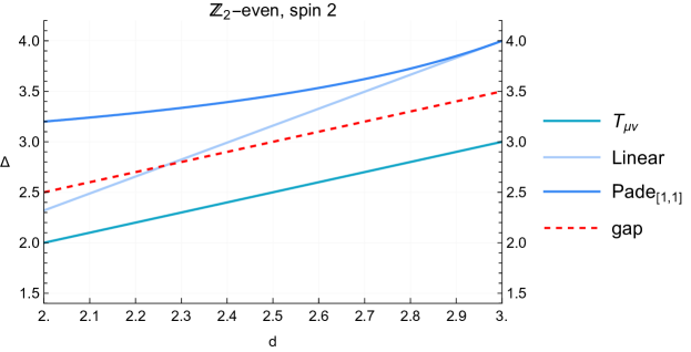
Figure 7: The first two ${\mathbb{Z}}_{2}$-even operators at spin $2$. We impose the gap assumption $\Delta_{T^{\prime}}\geqslant d+0.5$ (dashed red). The linear extrapolation of the one-loop dimension of the next operator seems to violate this, however assuming that it connects to the second spin-2 operator in $d=2$ gives a Padé_[1,1] approximant that is safely above our assumption.

In the preliminary study, we impose this gap in using the $\{\phi,\phi^{2}\}$ system, but find that it is not sufficient to isolate the theory. This is unsurprising given that the free-theory OPE coefficient $\lambda^{2}_{\phi\phi^{2}\phi^{5}}=0$, meaning that the $\{\phi,\phi^{2}\}$ system might not be sensitive enough to detect to the presence or not of $\phi^{5}$. Including $\phi^{3}$ as external would solve this, since $\lambda^{2}_{\phi^{2}\phi^{3}\phi^{5}}=10$ in the free theory (see (22)), hence we expect that the full $\{\phi,\phi^{2},\phi^{3}\}$ system should be sensitive to gap assumptions excluding $\phi^{5}$. We discuss the precise values for the gap assumptions below.

Finally, following other bootstrap works we also impose a gap in the spin-2 sector after the stress-tensor. We choose this gap to be $\frac{1}{2}$, compatible with the perturbative spectrum if we assume that the subleading spin-2 operator continues in a regular way to the subleading spin-2 operator in $d=2$, see figure 7.

4.2 Preliminary study from two-operator system

We now report the results from the preliminary study, in which we considered the $\{\phi,\phi^{2}\}$ system, i.e. using one ${\mathbb{Z}}_{2}$-odd and one ${\mathbb{Z}}_{2}$-even external scalar. This is the system (48) used in multiple studies for the Ising CFT, however, we now imposed completely different gap assumptions. We focused on $d=2.75$ and assumed

$$\Delta_{e} >1.6\,,$$ (53)

$$\Delta_{o} \in[1.1,1.6]\cup[3.5,\infty)\,,$$ (54)

where $\Delta_{e}$ and $\Delta_{o}$ represent any subleading operators in the ${\mathbb{Z}}_{2}$-even and ${\mathbb{Z}}_{2}$-odd representations. The scan parameters were $(\Delta_{\phi},\Delta_{\phi^{2}})$. The result of this study is a rather wide peninsula, starting close to (but not including) the free-theory point $(0.375,\,0.75)$ and extending towards the upper-right. We do not reproduce here.

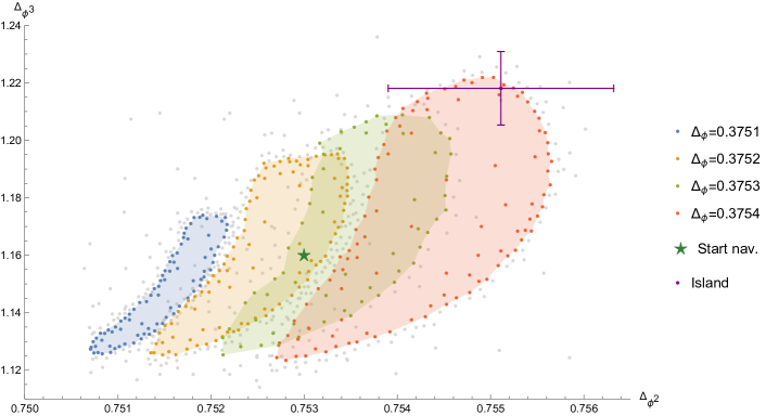
Figure 8: Results of preliminary study. Allowed regions for $(\Delta_{\phi^{2}},\Delta_{\phi^{3}})$ with fixed $\Delta_{\phi}$ from the two-correlator system. For comparison, we also show in purple (with error bars) the island found later using the three-correlator system with $\Delta_{\phi}\in[0.37526,0.37555]$, and the green star which is the start of the navigator run, (69), with $\Delta_{\phi}=0.3753$.

Next, still using the $\{\phi,\phi^{2}\}$ system, we added $\Delta_{\phi^{3}}$ as another scan parameter by replacing the interval $[1.1,1.6]$ with the exchange of an operator with fixed dimension $\Delta_{\phi^{3}}$. The assumptions were

$$\Delta_{e} >1.6\,,$$ (55)

$$\Delta_{\phi^{3}}\! \ \quad\text{isolated exchange},$$ (56)

$$\Delta_{o} >3.5\,,$$ (57)

$$\Delta_{T^{\prime}} >d+0.5=3.25\,,$$ (58)

where $\Delta_{T^{\prime}}$ denotes any operator after the stress-tensor in the ${\mathbb{Z}}_{2}$-even spin-2 sector. We fixed $\Delta_{\phi}$ to a few different values and looked for allowed regions in the variables $(\Delta_{\phi^{2}},\Delta_{\phi^{3}})$ using a Delaunay scan. We finished the scans after a rough outline of the allowed region was observed, leading to the following number of points.

$$\Delta_{\phi} =0.3751:\ \text{\small 85 allowed, 115 ruled out,} \Delta_{\phi} =0.3752:\ \text{\small 103 allowed, 127 ruled out,}$$ (59)

$$\Delta_{\phi} =0.3753:\ \text{\small 60 allowed, 76 ruled out,} \Delta_{\phi} =0.3754:\ \text{\small 104 allowed, 118 ruled out.}$$ (60)

The implementation of the Delaunay scan was done straightforwardly in Simpleboot.

The result of this search is displayed in figure 8. Imagining the colour (value of $\Delta_{\phi}$) as a third direction, this picture represents a widening three-dimensional peninsula. Looking only at the extension in $\Delta_{\phi^{2}}$ at fixed $\Delta_{\phi}$, the size of this peninsula is similar in size to the one derived without including $\Delta_{\phi^{3}}$.

4.3 Three-operator system and navigator minimisation

This section represents our main numerical effort. We considered a system with three external operators: $\{\phi,\phi^{2},\phi^{3}\}$ implemented as odd/even/odd scalars of an imposed global ${\mathbb{Z}}_{2}$ symmetry. Using Autoboot Go:2019lke ; Go:2020ahx , the crossing equations for this system were generated and imported to Simpleboot. There are 17 crossing equations (compared to 5 for $\{\phi,\phi^{2}\}$), four choices of quantum numbers (${\mathbb{Z}}_{2}$-even/odd and $(-1)^{\ell}$ even/odd), and the vectors $\vec{{\bm{\mathsf{V}}}}_{Q}$ of matrices of (47) have size $4\times 4$, $2\times 2$, $2\times 2$ and $1\times 1$, see appendix A.1.

We used Simpleboot to perform a navigator scan following Reehorst:2021ykw . Specifically, we used the “sigma navigator” which is automatically constructed in Simpleboot. For the gap assumptions, we used the unitarity bounds (49), except for the following cases:

$$\mathscr{D}_{+,0}=[\Delta_{e},\infty),\qquad\mathscr{D}_{-,0}=[\Delta_{o},\infty),\qquad\mathscr{D}_{+,2}=[d+\tfrac{1}{2},\infty),$$ (61)

We also imposed the presence of the stress-tensor with OPE coefficients proportional to the external scaling dimensions $(\lambda_{\phi\phi T},\lambda_{\phi\phi^{3}T},\lambda_{\phi^{2}\phi^{2}T},\lambda_{\phi^{3}\phi^{3}T})\propto(\Delta_{\phi},0,\Delta_{\phi^{2}},\Delta_{\phi^{3}})$.

The gaps were chosen in a way compatible with Padé approximants, based on the identification (see table 4) between the operators in the ${\varepsilon}$-expansion and those in $d=2$. Allowing for some margin, we selected the gaps

$$d =2.75:\quad\Delta_{e}=1.6,\quad\Delta_{o}=3.5,$$ (62)

$$d =2.75:\quad\Delta_{e}=1.35,\quad\Delta_{o}=3.5,$$ (63)

see figure 2. Finally, we used the following starting points for our three-parameter navigator runs:

$$d =2.75:\quad p_{\mathrm{init.}}=(0.3753,0.753,1.16),$$ (64)

$$d =2.5:\quad p_{\mathrm{init.}}=(0.25217,0.5223,0.984).$$ (65)

For $d=2.75$, this was chosen as a central point within figure 8, and for $d=2.5$, we used Padé approximants together with an allowed point in $d=2.75$ to select the initial point. Alternatively, the Padé approximants (20) alone could have been used directly as starting points.

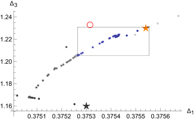
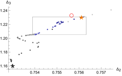
Figure 9: Navigator run in $d=2.75$, giving a complementary view to figure 4.

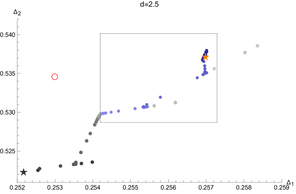
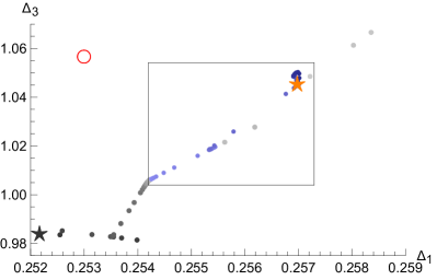
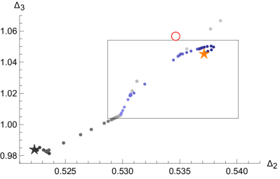
Figure 10: Navigator run in $d=2.5$, using the same notation as figure 4.

Results

Our navigator runs terminated after $134$ and $113$ iterations in $d=2.75$ and $d=2.5$ dimensions respectively, arriving at the following final points

$$d=2.75: \qquad(0.3755406408,\,0.7561071048,\,1.230056059),$$ (66)

$$d=2.5: \qquad(0.2569800178,\,0.5371399927,\,1.0454992842).$$ (67)

We visualise the runs in figures 9 and 10 respectively. We also present a summary of the setup and results in table 5.

Table 5: Some operators relevant for numerics, alongside our bounds and imposed gaps. The gaps in red did not lead to the isolation of the theory.

${\mathcal{O}}$	${\varepsilon}$-exp		$d=2.75$	$d=2.5$	$d=2.25$	$d=2$
$\phi$	$[\tfrac{1}{2}-\tfrac{{\varepsilon}}{2}]\!+\!\frac{{\varepsilon}^{2}}{1000}$​​ ​​	Padé2,2	$0.37531$	$0.25299$	$0.13990$	$0.075$
		Bound	$[0.37526,0.37555]$	$[0.25419,0.25729]$	NA	NA
$\phi^{2}$	$[1-{\varepsilon}]+\frac{4{\varepsilon}^{2}}{125}$	Padé2,2	$0.75566$	$0.53465$	$0.34835$	$0.2$
		Bound	$[0.75390,0.75632]$	$[0.52870,0.54013]$	NA	NA
$\phi^{3}$	$[\tfrac{3}{2}-\tfrac{3{\varepsilon}}{2}]+\frac{{\varepsilon}}{5}$	Padé2,1	$1.23347$	$1.05722$	$0.94354$	$0.875$
		Bound	$[1.20529,1.23098]$	$[1.00395,1.05415]$	NA	NA
$\phi^{4}$	$[2-2{\varepsilon}]+\frac{4{\varepsilon}}{5}$	Padé2,2	$1.74734$	$1.53744$	$1.35699$	$1.2$
		Gap	$1.6$	$1.35$	$1.15$; $1.3$​	$1.1$; $1.15$
$\phi^{6}$	$[3-3{\varepsilon}]+4{\varepsilon}$	Padé1,2	$3.04548$	$3.03431$	$3.01787$	$3$
$\phi^{7}$	$[\tfrac{7}{2}-\tfrac{7{\varepsilon}}{2}]+7{\varepsilon}$	Padé1,2	$3.74737$	$3.85975$	$3.96631$	$4.075$
		Gap	$3.5$	$3.5$	$3.7$; $3.8$	$3.9$; $4.025$​

Navigator behaviour

To give further details on the navigator run, we present three sets of plots showing properties of the navigator as a function of the iteration step $i$. Figure 11 shows the navigator value $|\mathcal{N}|$ as a function of $i$, figure 12 the gradient $|\nabla\mathcal{N}|$, and figure 13 the step length. In all of these plots, gray points are those with positive navigator value (disallowed), and purple with negative (allowed).

We see that the runs in $d=2.75$ and $d=2.5$ dimensions are qualitatively similar. In both cases, the approach towards the allowed region and then towards the minimum inside the allowed region is not uniform – the navigator has some plateaus with small step length, and then some phases with rather long step length. In the way out of such plateau, the step length is increased in an approximate geometric progression.

4.4 Extremising external scaling dimensions

Next, after finding allowed points and ultimately the navigator minima, we started six searches per value of $d$, with the objective of maximising/minimising in each of the parameter directions. All of these runs terminated, meaning that we obtained closed intervals in $(\Delta_{\phi},\Delta_{\phi^{2}},\Delta_{\phi^{3}})$ containing the navigator minimum, thus the delimitations of a bootstrap island. These intervals were reported in equations (2)–(3) in the introduction, and are also given in table 5 here.

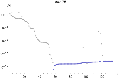
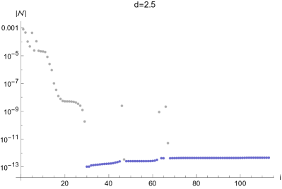
Figure 11: Navigator value.

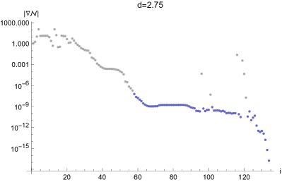
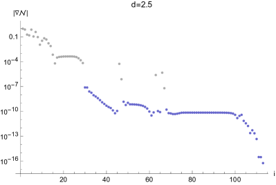
Figure 12: Gradient of navigator.

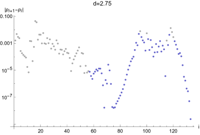
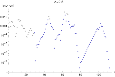
Figure 13: Step lengths.

In figures 15 and 16 in appendix A.2 we show all allowed points in $d=2.75$ and $d=2.5$, from the minimise-navigator run, and the extremisation runs. Although we did not map out the precise shape of the island, these plots indicate that is has an elongated shape.

To get a suitable estimate on how small/large our islands are, we change variables and display them in the space of anomalous dimensions. For $\phi^{k}$, we define the anomalous dimension by $\gamma_{\phi^{k}}=\Delta_{\phi^{k}}-k\frac{d-2}{2}$. In these variables, our islands correspond to the intervals

$$d=2.75 : \gamma_{\phi} \in[0.00026,\,0.00055], \gamma_{\phi^{2}} \in[0.00390\,,0.00632], \gamma_{\phi^{3}} \in[0.08029,\,0.10598],$$

$$d=2.5 : \gamma_{\phi} \in[0.00419,\,0.00729], \gamma_{\phi^{2}} \in[0.0287,\,0.04013], \gamma_{\phi^{3}} \in[0.25395,\,0.30415].$$ (68)

Thus we can observe that the islands we have found are rather large in this scale.

4.5 Run-off in $\bm{d=2.25}$ and $\bm{d=2}$

Based on the success in $d=2.75$ and $d=2.5$, we attempted a similar setup for $d=2$ and $d=2.25$ dimensions. We used the same algorithm and the same derivative-order as above, but adapted the gaps and starting points appropriately. Neither of these runs terminated at a navigator minimum – at the beginning of the runs they looked similar to the successful runs in figures 12–13, but after reaching allowed points, the navigator showed quick runoffs towards larger values of all parameters $(\Delta_{\phi},\Delta_{\phi^{2}},\Delta_{\phi^{3}})$. This indicates that there are no islands in these dimensions with the current setup, but instead “peninsulas.”

The gaps we used were the following:

$$d=2.25 :\quad\Delta_{e}=1.15,\ \Delta_{o}=3.7\ \text{(attempt 1)},\quad\Delta_{e}=1.3,\ \Delta_{o}=3.8\ \text{(attempt 2)},$$ (69)

$$d=2 :\quad\Delta_{e}=1.1,\ \Delta_{o}=3.9\ \text{(attempt 1)},\quad\Delta_{e}=1.15,\ \Delta_{o}=4.025\ \text{(attempt 2)},$$ (70)

see also table 5. We also tried a few different starting points.

Although we the lack of islands as a disappointment, we make a generic note peninsulas can still have some meaning as an indication of the existence of CFTs Chester:2016wrc ; Chester:2022hzt . If such peninsula is stable against varying some assumptions or increasing the derivative-order, it may be an indication that a theory might be close to saturating the bound. In that case, one could minimise one direction, say $\Delta_{\phi}$, and take that minimum as an approximate proxy for the theory.

4.6 Extremal spectrum

As a final step, we can extract an estimate of the spectrum using the extremal functional method ElShowk:2012hu ; El-Showk:2014dwa . We choose to do this at the final navigator point in $d=2.75$ and $d=2.5$ dimensions.

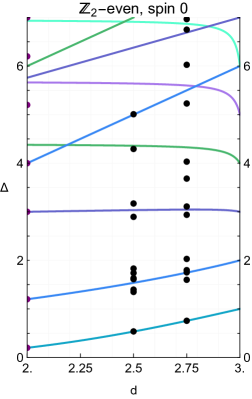
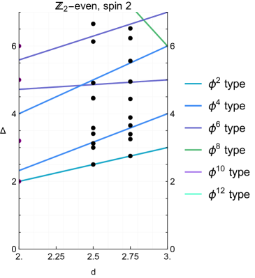
Figure 14: Spectra for ${\mathbb{Z}}_{2}$-even operators of spin 0 and spin 2. For the first three scalar operators, we show the Padé approximants (20). For the remaining scalar operators of form $\phi^{2k}$ we show $\text{Pad\'{e}}_{1,1}$ and for the rest we show $O({\varepsilon})$ truncated results.

In figure 14 we show ${\mathbb{Z}}_{2}$-even operators of spin 0 and 2. In this figure, we show the extremal spectra alongside perturbative estimates (our Padé approximants (20) for $\phi^{2k}$, $k=1,2,3$, Padé_1,1 for $k>3$, and linear for other operators). More extremal spectra are shown in figures 17, 18 and 19 in appendix A.3.

We can see that the extremal spectrum contains many points near our estimates, but the spread is large and there are many more number points than the expected number of operators. Compared to other studies, our extremal spectrum is disappointing and not very useful. For instance, in Henriksson:2022gpa for the Ising CFT, the structure of many nearby zeroes was not observed. It should be noted that Henriksson:2022gpa was performed with much higher numerical precision, $\Lambda=30$ instead of $\Lambda=19$, and the navigator minimum found there was inside much smaller islands than those found here.

4.7 Comparison with previous results

We would like to compare our results with the literature, however not much data is available at intermediate dimensions $d$. For $\Delta_{\phi}$ we can compare with figure 3 of Codello:2012sc , and for $\Delta_{\phi^{2}}$ with figure 4 of Codello:2014yfa (who also gave $\Delta_{\phi^{4}}$). Both these are results from the non-perturbative RG. Using the relations $\Delta_{\phi}=\frac{d-2}{2}+\frac{1}{2}\eta$, $\Delta_{\phi^{2}}=d-y_{1,3}$ and $\Delta_{\phi^{4}}=d-y_{2,3}$, the results in Codello:2012sc ; Codello:2014yfa translate to

$$d =2.75: \Delta_{\phi} =0.385\,, \Delta_{\phi^{2}} =0.754\,, \Delta_{\phi^{4}} =1.77\,,$$ (71)

$$d =2.5: \Delta_{\phi} =0.292\,, \Delta_{\phi^{2}} =0.524\,, \Delta_{\phi^{4}} =1.62\,.$$ (72)

We can see that especially $\Delta_{\phi}$ is rather off from our results. We do not take this disagreement as a sign of issues with our results, noting that the non-perturbative RG results deviate substantially also from the exact results in two dimensions: $\eta=0.31$ instead of $0.15$, $y_{1,3}=1.90$ instead of $1.80$ and $y_{2,3}=0.35$ instead of $0.8$.

4.8 Comments and possible improvements

Let us discuss a few potential improvements of the current setup, however beyond the scope of the present article. Some technical issues are deferred to appendix A.4.

Navigator vs other implementations

The navigator approach is very useful for large dimensionality of the search space and for finding small bootstrap islands. However, we observed that it required many iterations inside the allowed region to find the minimum. Moreover, the scans to minimise and maximise along the directions in parameter space also required many iterations. One option for mapping out the shape of the allowed region is to go back to a Delaunay scan (with surface-cutting algorithm for OPE ratios) after finding an allowed point, working in transformed variables where the island is less elongated. This was done e.g. in Chang:2024whx which studied the Ising CFT with the mixed $\{\phi,\phi^{2},T_{\mu\nu}\}$ system. A strategic choice of starting points may also reduce the number of iterations needed, see appendix A.4.

Another way to minimise the number of iterations (or rather the computational time at each iteration) is to use the Skydiving algorithm Liu:2023elz . However, it was not available at the beginning of this project, and our attempts to use it were not successful, probably due to the need of fine-tuning some internal parameters.

Preliminary study with more observables

Here we observed that the three-parameter scan $(\Delta_{\phi},\Delta_{\phi^{2}},\Delta_{\phi^{3}})$ was not enough to find an island in $d=2$ and $d=2.25$ dimensions. A future direction is to try more sophisticated setups. The most direct is to include dimensions of exchanged operators (e.g. $\phi^{4}$) and/or OPE ratios in the scan. The author has experimented with a few of these setups, including fixing one OPE ratio (see footnote 17), and a seven-parameter scan including both $\Delta_{\phi^{4}}$ and all OPE ratios of external operators. For the latter, we expect an interpolation between the 3d values (22)

$$\frac{1}{\lambda_{\phi\phi\phi^{2}}}\left(\lambda_{\phi\phi\phi^{2}},\lambda_{\phi^{2}\phi^{2}\phi^{2}},\lambda_{\phi\phi^{3}\phi^{2}},\lambda_{\phi^{3}\phi^{3}\phi^{2}}\right)=\{{1,2,1.22474488,3}\},$$ (73)

and the 2d exact values (40)

$$\frac{1}{\lambda_{\sigma\sigma\epsilon}}\left(\lambda_{\sigma\sigma\epsilon},\lambda_{\epsilon\epsilon\epsilon},\lambda_{\sigma\sigma^{\prime}\epsilon},\lambda_{\sigma^{\prime}\sigma^{\prime}\epsilon}\right)=\{1,0,0.546178,0\}.$$ (74)

Although promising, to perform a complete study with this system requires computational resources beyond the scope of this study.

Obtaining a better extremal spectrum

Here we discuss how the estimate of the spectrum might be improved. First, we only used a single point for the extremal spectrum, chosen at the minimum of the “sigma navigator” that we used here. This minimum was found quite far from the centre of the island, in disagreement with a hope that the navigator minimum should represent “the most allowed point” and that the island should shrink in a rather uniform way. To get a better estimate of the spectrum, other methods could be employed. Perhaps the GFF navigator would produce a minimum more central in the island and therefore a more realistic spectrum. One could also use the sampling method of Simmons-Duffin:2016wlq (also used in Liu:2020tpf ; Atanasov:2022bpi ), which amounts to selecting a sample of allowed points and extract the extremal spectrum at each point in the sample. Then one performs a statistical analysis where the operator dimensions that are relatively stable across the sample are retained, and their variation is used as an estimate of the error.

5 Discussion and outlook

In this paper, we have studied the tricritical Ising CFT in the range $2\leqslant d<3$, and obtained bootstrap islands in $d=2.75$ and $d=2.5$ dimensions. We performed a targeted bootstrap study, meaning that we aimed specifically at isolating a target CFT rather than deriving general bounds. To this end, we reviewed the perturbative data in section 2, and also supplemented the literature with a small survey of the low-lying spectrum using the one-loop dilatation operator (section 2.3). We also summarised the bootstrap method in section 3, with the aim of explaining in general terms how recent bootstrap technology can be used to study a target theory.

The islands we found agree well with Padé approximants connecting the $3-{\varepsilon}$ expansion to the exact values in $d=2$, see figures 2–3. This gives direct evidence in favour of the anticipated scenario that the minimal models $\mathcal{M}_{k+2,k+1}$ are continuously connected to $\phi^{2k}$ theory with upper critical dimension $d_{c}(k)=\frac{2k}{k-1}$, here for $k=3$. We now discuss various open directions.

5.1 How to find islands in $\bm{d=2}$ and $\bm{d=2.25}$?

We still failed to isolate the theory in $d=2$ dimensions, which means that to date the only 2d CFT to be isolated to a bootstrap island is the Ising CFT delaFuente:2019hbl . This contrasts the wealth of exact results available for 2d CFTs DiFrancesco:1997nk , and it would be interesting to understand better what the obstructions are. It is possible that a more judicious choice of assumptions would have isolated our target theory. For instance, one could demand that the stress-tensor is exchanged with the central charge fixed to $c=\frac{7}{10}$; the tricritical Ising is the only unitary CFT with that central charge. We did not attempt such judicious assumptions since ultimately the goal here was to develop and test methods that can apply to a wider set of theories, including those where we do not have exact results.

With this restriction taken into account, there are still some ideas that would be interesting to attempt. One is to experiment with different assumptions for spinning operators, where we only put a gap above the stress-tensor of $\frac{1}{2}$ (c.f. equation (58) and figure 7). The paper Li:2017kck nicely discussed how various assumptions in a single-correlator bootstrap system contributed to the isolation of several theories in 3d, including Ising, super-Ising and $O(3)$. One could also try with improved numerical strength (derivative-order $\Lambda$), and/or use improved numerical algorithms. The SDPB code has recently been updated to run faster, see Chang:2024whx , which may facilitate increased precision. It is possible that purely increasing $\Lambda$, keeping the same setup as here, will in fact isolate the theory to islands in $d=2$ and $d=2.25$, just like some islands in the literature cannot be obtained with too low $\Lambda$, e.g. in Kousvos:2021rar .

5.2 Perturbative computations for future bootstrap studies

One motivation for this work was to execute a complete sequence of steps to approach a specific target theory with the bootstrap. Although we discussed tricritical theories here, some lessons from this work should also apply to other systems – some practical and technical issues are discussed in section 4.8 and appendix A.4. An important target for the bootstrap is experimentally relevant $\phi^{4}$ theories Pelissetto:2000ek , some of which have not yet been isolated to precision islands with the bootstrap. Previous bootstrap studies of these theories Stergiou:2018gjj ; Kousvos:2018rhl ; Stergiou:2019dcv ; Kousvos:2019hgc ; Henriksson:2020fqi ; Kousvos:2021rar ; Kousvos:2022ewl ; Henriksson:2021lwn ; Reehorst:2024vyq have shown many suggestive features, which would be interesting to study further.

An important ingredient in our work is good perturbative estimates. Their role is to provide estimates for the target theory, and more generally also for known “competing” theories. Since the bootstrap is sensitive to many exchanged operators, not just those giving measurable critical exponents, we are interested in good estimates for a large portion of the spectrum, including spinning operators and operators in non-singlet global-symmetry representations.

Here we used a combination of multiloop results for low-lying operators, and a systematic study of the one-loop dilatation operator. This programme can also be executed for complicated global symmetry, such as the cubic $\phi^{4}$ theory Bednyakov:2023lfj . A collection of such data facilitates a flexible choice of gap assumptions, and at small ${\varepsilon}$ the perturbative estimates can be taken to be rather reliable. Using a set of gap assumptions, one can perform a bootstrap study first at small ${\varepsilon}$, and then increase towards physically interesting values of $d$. Such tracking strategy across $d$ was recently executed for $\phi^{4}$ theories with $O(m)\times O(n)$ symmetry Reehorst:2024vyq .

The current perturbative state of the art is multi-loop results for low-lying operators only, complemented with one-loop results for more larger parts of the spectrum. It would be desirable to go beyond this, with a study of multi-loop anomalous dimensions of arbitrary composite operators. Steps towards this are taken in LoopsBootstrap , where composite operators are renormalised in $4-{\varepsilon}$ dimensions using Feynman diagrams and techniques for operator bases from effective field theory Cao:2021cdt . It would be nice to extend this computation to $3-{\varepsilon}$ dimensions.

To generate perturbative results for theories with various global symmetries, it is convenient to work with interactions with “open field indices,” like in Bednyakov:2021ojn for $\phi^{4}$ theories. Translating this idea to our case implies working with the general Lagrangian density

$$\mathcal{L}\!=\!u_{0}+u_{1}^{i}\phi_{i}+\frac{u_{2}^{ij}\!}{2}\phi_{i}\phi_{j}+\frac{u_{3}^{ijk}\!\!}{3!}\phi_{i}\phi_{j}\phi_{k}+\frac{u_{4}^{ijkl}\!\!}{4!}\phi_{i}\phi_{j}\phi_{k}\phi_{l}+\frac{u_{5}^{ijklm}\!\!\!}{5!}\phi_{i}\phi_{j}\phi_{k}\phi_{l}\phi_{m}+\frac{u_{6}^{ijklmn}\!\!\!\!}{6!}\phi_{i}\phi_{j}\phi_{k}\phi_{l}\phi_{m}\phi_{n}$$ (75)

and computing beta functions for all interactions $u_{i}$ in $3-{\varepsilon}$ dimensions. It should be possible to perform this computation by recycling diagrammatic technology from Hager1999 ; Hager:2002uq . By using group theory, results for many different theories with different global symmetry could then be extracted.

5.3 Tricritical $\bm{O(n)}$ models

One of the motivations for this work is to lay the ground for future works on tricritical CFTs with global symmetry $O(n)$ Pisarski:1982vz ; Bardeen:1983rv ; Amit:1984ri ; David:1984we ; Gudmundsdottir:1984vyf ; Gudmundsdottir:1984rr ; David:1985zz ; Hager1999 ; Hager:2002uq ; Kaplan:2009kr ; Yabunaka:2017uox ; Osborn:2017ucf ; Katsis:2018bvc ; Goykhman:2020ffn , since the literature on these theories contains some interesting results. It is known that the $3-{\varepsilon}$ expansion for the tricritical $O(n)$ model does not have a well-behaved large-$n$ limit. Specifically, leading order perturbative data suggest that this expansion is only valid for $\varepsilon<\frac{36}{\pi^{2}n}\approx\frac{3.6}{n}$ . In Yabunaka:2017uox , it was proposed with motivation from non-perturbative RG that the curve ${\varepsilon}\approx\frac{3.6}{n}$ ends at some finite $n\approx 19$. Above this value, the tricritical $O(n)$ CFT should annihilate with a new non-perturbative fixed-point. Below this value, Yabunaka:2017uox predicts that the theory continues to exist, and by going around the point $(d,n)\approx(2.8,19)$ to the bottom-left and then towards large $n$ one reaches another new non-perturbative fixed-point. It would be very interesting to study these putative non-perturbative CFTs with the bootstrap, where a mixed system $\{\varphi,\varphi^{2}_{S},\varphi^{3}_{V}\}$ inspired by this paper might be the right tool. See Yabunaka:2018mju ; Defenu:2020cji ; Yabunaka:2021fow for further comments, and Hawashin:2024dpp ; Komargodski:2024zmt for work on other putative new CFTs of similar type.

5.4 Multicritical models

Another direction is to bootstrap the higher multicritical theories. It would be nice to establish with the bootstrap the connection between theories with $\phi^{2k}$ interaction near their upper critical dimensions, and the minimal models $\mathcal{M}_{k+2,k+1}$. In appendix D we collect some results for these theories.

Allowing for multicritical theories with global symmetry gives a plethora of opportunities. A collection of perturbative fixed-points of this class, based on discrete subgroups of $O(N)$, was discussed in Zinati:2019gct , see also Codello:2020mnt ; Kapoor:2021lrr ; BenAliZinati:2021rqc . It is not established what happens to these theories as ${\varepsilon}$ is increased, and likewise which two-dimensional CFTs belong to families of CFTs extending above $d=2$ dimensions. A related question, for the tricritical model considered here, is whether its supersymmetric version can be bootstrapped and continued above two dimensions to make contact with the three-dimensional minimal $\mathcal{N}=1$ supersymmetric Ising CFT Bashkirov:2013vya ; Iliesiu:2015qra ; Rong:2018okz ; Atanasov:2022bpi , see also Fei:2016sgs .

Appendix A Details on numerics and more results

In this appendix we give some bulky expressions and give further details on the numerics.

A.1 Crossing equations and bootstrap settings

The bootstrap equation (47) in our system with one ${\mathbb{Z}}_{2}$-even and two ${\mathbb{Z}}_{2}$-odd operators was generated in Autoboot Go:2019lke ; Go:2020ahx and takes the form

$$0=\vec{V}_{\text{OPE}}+\sum_{{\mathcal{O}}_{+,+}}\bm{\lambda}_{++}^{T}\vec{{\bm{\mathsf{V}}}}_{+,+}\bm{\lambda}_{++}+\sum_{{\mathcal{O}}_{+,-}}\lambda_{13{\mathcal{O}}}^{2}V_{+,-}+\sum_{{\mathcal{O}}_{-,+}}\bm{\lambda}_{-+}^{T}\vec{{\bm{\mathsf{V}}}}_{-,+}\bm{\lambda}_{-+}+\sum_{{\mathcal{O}}_{-,-}}\bm{\lambda}_{--}^{T}\vec{{\bm{\mathsf{V}}}}_{-,-}\bm{\lambda}_{--},$$ (76)

where we labelled the sectors by ${\mathbb{Z}}_{2}$ representation $\pm$ and spin parity $(-1)^{\ell}$. In this expression, the vectors of matrices are given by

$$\vec{{\bm{\mathsf{V}}}}_{+,+} =\bigg{\{}\left(\begin{smallmatrix}F_{1111}&0&0&0\\ 0&0&0&0\\ 0&0&0&0\\ 0&0&0&0\\ \end{smallmatrix}\right),\tfrac{1}{2}\!\left(\begin{smallmatrix}0&{F_{1113}}&0&0\\ {F_{1113}}&0&0&0\\ 0&0&0&0\\ 0&0&0&0\\ \end{smallmatrix}\right),\tfrac{1}{2}\!\left(\begin{smallmatrix}0&0&H_{1122}&0\\ 0&0&0&0\\ H_{1122}&0&0&0\\ 0&0&0&0\\ \end{smallmatrix}\right),\tfrac{1}{2}\!\left(\begin{smallmatrix}0&0&F_{1122}&0\\ 0&0&0&0\\ F_{1122}&0&0&0\\ 0&0&0&0\\ \end{smallmatrix}\right),$$

$$\qquad\tfrac{1}{2}\!\left(\begin{smallmatrix}0&0&0&H_{1133}\\ 0&-2H_{1331}&0&0\\ 0&0&0&0\\ H_{1133}&0&0&0\\ \end{smallmatrix}\right),\tfrac{1}{2}\!\left(\begin{smallmatrix}0&0&0&F_{1133}\\ 0&2F_{1331}&0&0\\ 0&0&0&0\\ F_{1133}&0&0&0\\ \end{smallmatrix}\right),\mathbf{0},\tfrac{1}{2}\!\left(\begin{smallmatrix}0&0&0&0\\ 0&0&H_{1322}&0\\ 0&H_{1322}&0&0\\ 0&0&0&0\\ \end{smallmatrix}\right),$$

$$\qquad\tfrac{1}{2}\!\left(\begin{smallmatrix}0&0&0&0\\ 0&0&F_{1322}&0\\ 0&F_{1322}&0&0\\ 0&0&0&0\\ \end{smallmatrix}\right),\mathbf{0},\left(\begin{smallmatrix}0&0&0&0\\ 0&F_{1313}&0&0\\ 0&0&0&0\\ 0&0&0&0\\ \end{smallmatrix}\right),\tfrac{1}{2}\!\left(\begin{smallmatrix}0&0&0&0\\ 0&0&0&F_{1333}\\ 0&0&0&0\\ 0&{F_{1333}}&0&0\\ \end{smallmatrix}\right),\left(\begin{smallmatrix}0&0&0&0\\ 0&0&0&0\\ 0&0&F_{2222}&0\\ 0&0&0&0\\ \end{smallmatrix}\right),$$

$$\qquad\tfrac{1}{2}\!\left(\begin{smallmatrix}0&0&0&0\\ 0&0&0&0\\ 0&0&0&{H_{2233}}\\ 0&0&{H_{2233}}&0\\ \end{smallmatrix}\right),\tfrac{1}{2}\!\left(\begin{smallmatrix}0&0&0&0\\ 0&0&0&0\\ 0&0&0&F_{2233}\\ 0&0&F_{2233}&0\\ \end{smallmatrix}\right),\mathbf{0},\left(\begin{smallmatrix}0&0&0&0\\ 0&0&0&0\\ 0&0&0&0\\ 0&0&0&F_{3333}\\ \end{smallmatrix}\right)\bigg{\}},$$ (77)

$$\vec{V}_{+,-} =\left\{0,0,0,0,H_{1331},-F_{1331},0,0,0,0,F_{1313},0,0,0,0,0,0\right\},$$ (78)

$$\vec{{\bm{\mathsf{V}}}}_{-,+} =\bigg{\{}\mathbf{0},\mathbf{0},\left(\begin{smallmatrix}-H_{1221}&0\\ 0&0\\ \end{smallmatrix}\right),\left(\begin{smallmatrix}F_{1221}&0\\ 0&0\\ \end{smallmatrix}\right),\mathbf{0},\mathbf{0},\left(\begin{smallmatrix}F_{1212}&0\\ 0&0\\ \end{smallmatrix}\right),\tfrac{1}{2}\left(\begin{smallmatrix}0&-{H_{1223}}\\ -{H_{1223}}&0\\ \end{smallmatrix}\right),\tfrac{1}{2}\left(\begin{smallmatrix}0&{F_{1223}}\\ {F_{1223}}&0\\ \end{smallmatrix}\right),$$

$$\qquad\tfrac{1}{2}\left(\begin{smallmatrix}0&{F_{1232}}\\ {F_{1232}}&0\\ \end{smallmatrix}\right),\mathbf{0},\mathbf{0},\mathbf{0},\left(\begin{smallmatrix}0&0\\ 0&-H_{2332}\\ \end{smallmatrix}\right),\left(\begin{smallmatrix}0&0\\ 0&F_{2332}\\ \end{smallmatrix}\right),\left(\begin{smallmatrix}0&0\\ 0&F_{2323}\\ \end{smallmatrix}\right),\mathbf{0}\bigg{\}},$$ (79)

$$\vec{{\bm{\mathsf{V}}}}_{-,-} =\bigg{\{}\mathbf{0},\mathbf{0},\left(\begin{smallmatrix}H_{1221}&0\\ 0&0\\ \end{smallmatrix}\right),\left(\begin{smallmatrix}-F_{1221}&0\\ 0&0\\ \end{smallmatrix}\right),\mathbf{0},\mathbf{0},\left(\begin{smallmatrix}F_{1212}&0\\ 0&0\\ \end{smallmatrix}\right),\tfrac{1}{2}\left(\begin{smallmatrix}0&-{H_{1223}}\\ -{H_{1223}}&0\\ \end{smallmatrix}\right),\tfrac{1}{2}\left(\begin{smallmatrix}0&{F_{1223}}\\ {F_{1223}}&0\\ \end{smallmatrix}\right),$$

$$\qquad\tfrac{1}{2}\left(\begin{smallmatrix}0&-{F_{1232}}\\ -{F_{1232}}&0\\ \end{smallmatrix}\right),\mathbf{0},\mathbf{0},\mathbf{0},\left(\begin{smallmatrix}0&0\\ 0&H_{2332}\\ \end{smallmatrix}\right),\left(\begin{smallmatrix}0&0\\ 0&-F_{2332}\\ \end{smallmatrix}\right),\left(\begin{smallmatrix}0&0\\ 0&F_{2323}\\ \end{smallmatrix}\right),\mathbf{0}\bigg{\}},$$ (80)

where $F_{ijkl}$ ($H_{ijkl}$) is the difference (sum) of conformal blocks involving the operators $\phi^{i},\phi^{j},\phi^{k},\phi^{l}$ (compare with (46)), and the vectors of OPE coefficients are given by $\bm{\lambda}_{++}=(\lambda_{11{\mathcal{O}}},\lambda_{13{\mathcal{O}}},\lambda_{22{\mathcal{O}}},\lambda_{33{\mathcal{O}}})^{T}$ and $\bm{\lambda}_{-+}=\bm{\lambda}_{--}=(\lambda_{12{\mathcal{O}}},\lambda_{23{\mathcal{O}}})^{T}$. Moreover, the OPE coefficient block is given by exchanging the operator $\phi^{2}$ in $Q=(+,+)$, the operators $\phi$ and $\phi^{3}$ in $Q=(-,+)$ and repackaging the resulting expression to the form

$$\vec{V}_{\text{OPE}}=\bm{\lambda}^{T}\vec{{\bm{\mathsf{V}}}}\bm{\lambda}\,,\qquad\bm{\lambda}=(\lambda_{112},\lambda_{123},\lambda_{222},\lambda_{233})^{T}.$$ (81)

This gives $\vec{{\bm{\mathsf{V}}}}$ of the form

$$\bigg{\{}\!\!\left(\begin{smallmatrix}F_{1111}(\Delta_{2})&0&0&0\\ 0&0&0&0\\ 0&0&0&0\\ 0&0&0&0\\ \end{smallmatrix}\right)\!,\tfrac{1}{2}\!\left(\begin{smallmatrix}0&{F_{1113}(\Delta_{2})}&0&0\\ {F_{1113}(\Delta_{2})}&0&0&0\\ 0&0&0&0\\ 0&0&0&0\\ \end{smallmatrix}\right)\!,\tfrac{1}{2}\!\left(\begin{smallmatrix}-2H_{1221}(\Delta_{1})&0&{H_{1122}(\Delta_{2})}&0\\ 0&-2H_{1221}(\Delta_{3})&0&0\\ {H_{1122}(\Delta_{2})}&0&0&0\\ 0&0&0&0\\ \end{smallmatrix}\right)\!,\ldots\bigg{\}}.$$ (82)

We also separate out the contribution from the stress-tensor and contract it with the OPE coefficient vector $\bm{\lambda}\propto(\Delta_{\phi},0,\Delta_{\phi^{2}},\Delta_{\phi^{3}})^{T}$, as dictated by the conformal Ward identities.

In Simpleboot, we use $\Lambda=19$, $\kappa=80$, $r_{N}=20$, and the following spins:

$$\mathscr{L}=\{0,1,2,3,\ldots,33,34,\,51,52\}$$ (83)

For the navigator SDPB runs, we used the settings:

--saveMiddleCheckpointMuThreshold=1e-8

--maxIterations=1000

--dualityGapThreshold=1e-25

--primalErrorThreshold=1e-15

--dualErrorThreshold=1e-15

--precision=1200

--initialMatrixScalePrimal=1e+20

--initialMatrixScaleDual=1e+20

--maxComplementarity=1e+70

A.2 Navigator islands

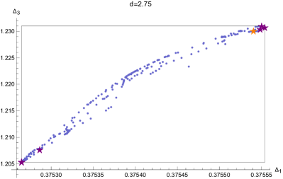
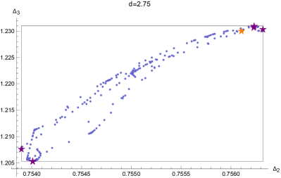
Figure 15: All allowed navigator points in $d=2.75$. Stars denote the end-points of navigator runs extremising the directions.

In figures 15 and 16 we present the results from our navigator runs to maximise/minimise along the parameter directions, giving the size of the navigator islands in $d=2.75$ and $d=2.5$ dimensions. They result from runs with the following number of points:

$$d =2.75\!: \Delta_{\phi} \ 119/119, \Delta_{\phi^{2}} \ 49/113, \Delta_{\phi^{3}} \ 133/67,$$ max/min : max/min : max/min : (84)

$$d =2.5\!: \Delta_{\phi} \ 40/94, \Delta_{\phi^{2}} \ 51/150, \Delta_{\phi^{3}} \ 48/127.$$ max/min : max/min : max/min : (85)

In the figures, all these runs are superimposed alongside the run to minimise the navigator. The extremisation runs terminated at the extrema reported in table 5 in the main text, and shown as purple stars in the figures.

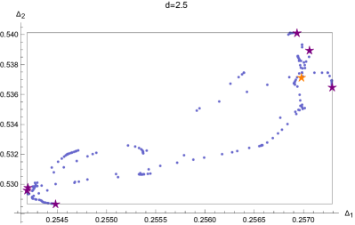
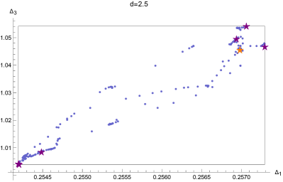
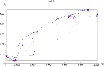
Figure 16: All allowed navigator points in $d=2.5$. Same description as figure 15.

A.3 Extremal spectra

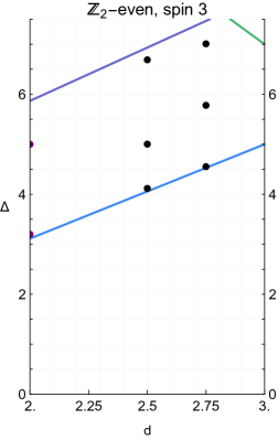
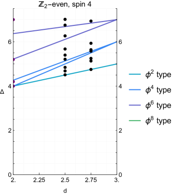
Figure 17: Spectra for ${\mathbb{Z}}_{2}$-even operators of spin 3 and spin 4. The perturbative spin-$3$ spectrum looks rather sparse. This is because there is no spin-3 primary with six fields and $\Delta=6$, since the corresponding primary in the free theory is involved in a multiplet recombination effect with the spin-4 broken current of dimension $5$.

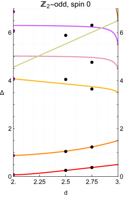
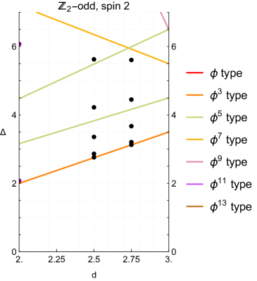
Figure 18: Spectra for ${\mathbb{Z}}_{2}$-odd operators of spin 0 and spin 2.

In figure 17 we show the extremal spectra for ${\mathbb{Z}}_{2}$-even operators of spin 3 and 4, complementing figure 14 in the main text. The ${\mathbb{Z}}_{2}$-odd extremal spectra are shown in figure 18 for spin 0 and 2, and in figure 19 for spin 3 and 4. As remarked in the main text, the extremal spectra show poor agreement with the perturbative estimates.

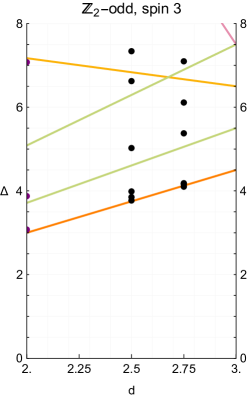
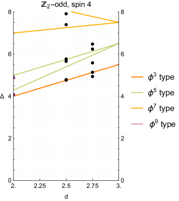
Figure 19: Spectra for ${\mathbb{Z}}_{2}$-odd operators of spin 3 and spin 4.

A.4 Running bootstrap in practice

Here we make a few remarks from the experience of running the bootstrap algorithms for this project. They represent some practical issues and are aspects to keep in mind for future similar studies.

• The scanning algorithm with Delaunay triangularisation is effective for regions with rounded shapes, while some bootstrap islands from the literature have been rather elongated. Especially at pointy regions at the end of such elongated regions the algorithm performs badly. This can be mitigated by manually adding points during the run (possible in Simpleboot), or by a change of variables to make the size of the expected island roughly equal in all directions, as done e.g. in Chester:2019ifh ; Chang:2024whx .

• In the navigator, one point is solved at the time before moving to the next iteration, meaning that a complete scan can extend over weeks. In this case, jobs might be killed by the cluster and have to be restarted. In Simpleboot, a job are restarted easily by moving the point to the evaluation queue, and if the job was terminated during an SDPB run, this leads to no problems. However, if the job was terminated at some other stage, for instance while the blocks were computed, it may corrupt some ancillary files which have to be deleted by hand.

• Using hot-starting (c.f. section 3.3), a check-point from a nearby iteration is loaded into SDPB, which can sometimes lead to stalling. Ultimately Simpleboot will detect this, delete the check-point and start a new SDPB run without check-point leading to significantly longer running time. This can be avoided by a manual intervention, in which we remove by hand the “bad” checkpoint and replace it with another (hopefully better) check-point from a nearby point.

• In this project, our runs to maximise/minimise along the directions in the scan space took significant number of iterations before even getting close to the relevant region, since our island was rather elongated. A simple proposal to reduce the total number of iterations is to first explore the extent of the island in both directions along just one axis, and then start the other scans from points near the two ends.

Appendix B Review of results from perturbative renormalisation

For convenience, we reproduce here the renormalisation constants and beta functions from Hager1999 ; Hager:2002uq , specialising to the case $n=1$. These papers constitute a six-loop renormalisation of the action (1), giving $O({\varepsilon}^{3})$ data for the operators $\phi$, $\phi^{2}$, $\phi^{4}$ and $\phi^{6}$. The beta function for $\lambda$ is

$$\beta(\bar{\lambda}) =-\mu\frac{{\partial}\bar{\lambda}}{{\partial}\mu}=-2\epsilon\bar{\lambda}+\frac{10\bar{\lambda}^{2}}{3}+\left(-\frac{45\zeta_{2}}{4}-\frac{281}{15}\right)\bar{\lambda}^{3}$$ (86)

$$\quad+\bar{\lambda}^{4}\left(\zeta_{2}\left(90\beta_{2}+\frac{2785}{12}+45\ln 2\right)+360\beta_{4}-\frac{525\zeta_{3}}{4}+\frac{3375\zeta_{4}}{16}+\frac{3643}{18}\right),$$ (87)

and the critical coupling is

$$\bar{\lambda}_{*} =\frac{3{\varepsilon}}{5}+\frac{9(675\zeta_{2}+1124){\varepsilon}^{2}}{5000}-\bigg{(}27\frac{5400\beta_{2}-1249+2700\ln(2)}{25000}\zeta_{2}$$

$$\qquad\qquad\qquad\qquad+\frac{2916\beta_{4}}{125}-\frac{1701\zeta_{3}}{200}+\frac{2187\zeta_{4}}{1600}-\frac{165519}{312500}\bigg{)}{\varepsilon}^{3},$$ (88)

where the bar denotes the absorption of factors of $32\pi^{2}$. In these expressions, $\zeta_{k}$ denote the usual Riemann zeta values, and $\beta_{k}$ denote the Dirichlet beta function $\sum_{n=0}^{\infty}(-1)^{n}/(2n+1)^{k}$.

Computing the field renormalisation constants and beta functions, and evaluating at the critical coupling $\bar{\lambda}_{*}$, gives

$$\gamma_{\phi} =\frac{{\varepsilon}^{2}}{1000}+\left(\frac{2279}{375000}+\frac{27\pi^{2}}{40000}\right){\varepsilon}^{3}+O({\varepsilon}^{4}),$$ (89)

$$\gamma_{\phi^{2}} =\frac{4{\varepsilon}^{2}}{125}+\left(\frac{513\zeta_{2}}{5000}+\frac{3866}{46875}\right){\varepsilon}^{3}+O({\varepsilon}^{4}),$$ (90)

$$\gamma_{\phi^{4}} =\frac{4{\varepsilon}}{5}+\frac{60750\zeta_{2}+72120}{75000}{\varepsilon}^{2}-\bigg{(}\frac{2592\beta_{4}}{125}-\frac{1701\zeta_{3}}{250}+\frac{2187\zeta_{4}}{800}$$

$$\quad\qquad+3\frac{5400\beta_{2}+1528+2025\ln 2}{3125}\zeta_{2}-\frac{77821}{234375}\bigg{)}{\varepsilon}^{3}+O({\varepsilon}^{4}),$$ (91)

$$\gamma_{\phi^{6}} =4{\varepsilon}-\frac{20250\zeta_{2}+33720}{5000}{\varepsilon}^{2}+\bigg{(}\frac{3888\beta_{4}}{25}-\frac{567\zeta_{3}}{10}+\frac{8019\zeta_{4}}{160}+\frac{655476}{15625}$$

$$\quad\qquad+{9}\frac{2700\beta_{2}+3169+1350\ln 2}{625}\zeta_{2}\bigg{)}+O({\varepsilon}^{4}).$$ (92)

Expressions for general $n$ are given in Hager:2002uq .

B.1 Other large expressions

Here we write explicitly a set of corrections to the OPE coefficients from Henriksson:2020jwk , where they were only given implicitly. Denoting $\mathcal{J}_{\ell}=\phi{\partial}^{\ell}\phi$, the OPE coefficients with $\phi$ are

$$\lambda_{\phi\phi\mathcal{J}_{\ell}}^{2}=\left(\lambda_{\phi\phi\mathcal{J}_{\ell}}^{\mathrm{free},3-{\varepsilon}}\right)^{2}\big{[}1+{\varepsilon}^{2}\alpha_{\ell}+O({\varepsilon}^{3})\big{]},$$ (93)

where

$$\alpha_{\ell}=\frac{15}{4(\ell-\frac{1}{2})(\ell+\frac{1}{2})^{2}}+\frac{\ell^{2}-4}{\ell^{2}-\frac{1}{4}}\big{[}S_{1}(\ell-1)-S_{1}(2\ell-1)\big{]}+S_{1}\left(\ell-\tfrac{1}{2}\right)+2\ln 2\,,$$ (94)

and

$$\left(\lambda_{\phi\phi\mathcal{J}_{\ell}}^{\mathrm{free},d}\right)^{2}=\frac{2\Gamma(\frac{d}{2}+\ell-1)^{2}\Gamma(d+\ell-3)}{\Gamma\left(\frac{d}{2}-1\right)^{2}\Gamma(\ell+1)\Gamma(d+2\ell-3)}$$ (95)

are the free OPE coefficients in $d$ dimensions. $S_{1}$ denotes the analytic continuation of the harmonic numbers. Despite the apparent appearance of $\ln 2$, the corrections $\alpha_{\ell}$ are rational numbers, $\alpha_{2}=\frac{23}{3750}$, $\alpha_{4}=\frac{9349}{1653750}$, etc.

Appendix C Character decompositions

In $d=3$ dimensions, we use the methods from Dolan:2005wy ; Henning:2017fpj to write the character decomposition of the spectrum of the free scalar field in terms of conformal primary operators. In table 6, we give the spectrum of parity-even operators. In this table we emphasised the contribution of certain operators: The multiplet of the stress tensor $T_{\mu\nu}$ is short in both the free and the interacting theory. The multiplets of $\phi$ and the currents $\mathcal{J}_{\ell}$ are short in the free theory, but long in the interacting theory. This means that certain primaries higher in the spectrum, denoted $E$ (equation-of-motion) are missing from the tricritical CFT. In table 7, we give the parity-odd spectrum. Notice in particular that the first parity-odd scalar has $\Delta=11$.

Table 6: Spectrum of parity-even operators in the theory of a free 3d scalar field. The horizontal axis denotes $\Delta$, the vertical axis $\ell$. $E$ denotes operators missing in the interacting theory due to equation-of-motion effects.

$8$																		$\!\!\!\mathcal{J}_{8}\!\!\!$	$2$	$4$	$5$	$6$
$7$																$0$	$1$	$2$	$3$	$\!\!\!\!\!E+2\!\!\!\!\!$	$4$	$6$
$6$														$\!\!\!\mathcal{J}_{6}\!\!\!$	$2$	$3$	$3$	$4$	$4$	$7$	$9$	$11$
$5$												$0$	$1$	$1$	$2$	$\!\!\!\!\!E+1\!\!\!\!\!$	$2$	$3$	$5$	$5$	$6$	$7$
$4$										$\!\!\!\mathcal{J}_{4}\!\!\!$	$1$	$2$	$2$	$2$	$2$	$4$	$4$	$5$	$5$	$8$	$11$	$14$
$3$								$0$	$1$	$1$	$1$	$E$	$1$	$1$	$2$	$2$	$2$	$3$	$5$	$6$	$7$	$8$
$2$						$T$	$1$	$1$	$1$	$1$	$1$	$2$	$2$	$2$	$2$	$3$	$4$	$5$	$5$	$7$	$9$	$12$
$1$				$0$	$0$	$0$	$0$	$0$	$0$	$0$	$0$	$0$	$0$	$0$	$1$	$1$	$1$	$1$	$3$	$3$	$4$	$4$
$0$	$\phi$	$1$	$1$	$1$	E	$1$	$1$	$1$	$1$	$1$	$1$	$2$	$2$	$2$	$2$	$3$	$3$	$4$	$4$	$5$	$5$	$7$
	$\frac{1}{2}$	$1$	$\frac{3}{2}$	$2$	$\frac{5}{2}$	$3$	$\frac{7}{2}$	$4$	$\frac{9}{2}$	$5$	$\frac{11}{2}$	$6$	$\frac{13}{2}$	$7$	$\frac{15}{2}$	$8$	$\frac{17}{2}$	$9$	$\frac{19}{2}$	$10$	$\frac{21}{2}$	$11$

Table 7: Spectrum of parity-odd operators in the theory of a free 3d scalar field. The horizontal axis denotes $\Delta$, the vertical axis $\ell$.

$8$																		$0$	$0$	$0$	$1$	$3$
$7$																$0$	$0$	$0$	$1$	$2$	$3$	$4$
$6$														$0$	$0$	$0$	$1$	$2$	$3$	$3$	$3$	$6$
$5$												$0$	$0$	$0$	$0$	$1$	$1$	$1$	$1$	$3$	$5$	$7$
$4$										$0$	$0$	$0$	$1$	$1$	$1$	$1$	$1$	$2$	$4$	$5$	$5$	$7$
$3$								$0$	$0$	$0$	$0$	$0$	$0$	$0$	$0$	$1$	$2$	$2$	$2$	$2$	$4$	$6$
$2$						$0$	$0$	$0$	$0$	$0$	$0$	$0$	$0$	$1$	$1$	$1$	$1$	$2$	$3$	$4$	$4$	$5$
$1$				$0$	$0$	$0$	$0$	$0$	$0$	$0$	$0$	$0$	$0$	$0$	$0$	$0$	$0$	$0$	$0$	$0$	$1$	$2$
$0$	$0$	$0$	$0$	$0$	$0$	$0$	$0$	$0$	$0$	$0$	$0$	$0$	$0$	$0$	$0$	$0$	$0$	$0$	$0$	$0$	$0$	$1$
	$\frac{1}{2}$	$1$	$\frac{3}{2}$	$2$	$\frac{5}{2}$	$3$	$\frac{7}{2}$	$4$	$\frac{9}{2}$	$5$	$\frac{11}{2}$	$6$	$\frac{13}{2}$	$7$	$\frac{15}{2}$	$8$	$\frac{17}{2}$	$9$	$\frac{19}{2}$	$10$	$\frac{21}{2}$	$11$

In $d=2$ we consider the torus partition function (42). Using the expressions for the characters given in Castro:2011zq , we expand each character up to level-10 descendants:

$$\chi_{vac} =\tilde{\chi}_{2,2}+\chi_{4,0}+\tilde{\chi}_{4,4}+\chi_{6,2}+2\tilde{\chi}_{6,6}+\chi_{8,0}+2\chi_{8,4}+3\tilde{\chi}_{8,8}+\chi_{9,9}+2\chi_{10,2}+3\chi_{10,6}$$

$$\quad+4\tilde{\chi}_{10,10}$$ (96)

$$\chi_{\phi_{2,2}} =\chi_{0,0}+\chi_{2,2}+\chi_{3,3}+\chi_{4,0}+\chi_{4,4}+\chi_{5,1}+2\chi_{5,5}+\chi_{6,0}+\chi_{6,2}+2\chi_{6,6}+\chi_{7,1}+2\chi_{7,3}$$

$$\quad+3\chi_{7,7}+\chi_{8,0}+2\chi_{8,2}+2\chi_{8,4}+4\chi_{8,8}+2\chi_{9,1}+2\chi_{9,3}+3\chi_{9,5}+5\chi_{9,9}+4\chi_{10,0}$$

$$\quad+2\chi_{10,2}+3\chi_{10,4}+4\chi_{10,6}+6\chi_{10,10}\,,$$ (97)

$$\chi_{\phi_{1,2}} =\chi_{0,0}+\chi_{3,3}+\chi_{4,4}+\chi_{5,5}+\chi_{6,0}+2\chi_{6,6}+\chi_{7,1}+2\chi_{7,7}+\chi_{8,0}+\chi_{8,2}+3\chi_{8,8}$$

$$\quad+\chi_{9,1}+2\chi_{9,3}+3\chi_{9,9}+\chi_{10,0}+2\chi_{10,2}+2\chi_{10,4}+5\chi_{10,10}\,,$$ (98)

$$\chi_{\phi_{2,1}} =\chi_{0,0}+\chi_{3,3}+\chi_{4,4}+\chi_{5,5}+\chi_{6,0}+2\chi_{6,6}+\chi_{7,1}+2\chi_{7,7}+\chi_{8,0}+\chi_{8,2}+2\chi_{8,8}$$

$$\quad+\chi_{9,1}+2\chi_{9,3}+4\chi_{9,9}+\chi_{10,0}+2\chi_{10,2}+2\chi_{10,4}+4\chi_{10,10}\,,$$ (99)

$$\chi_{\phi_{3,2}} =\chi_{0,0}+\chi_{2,2}+\chi_{4,0}+2\chi_{4,4}+\chi_{5,5}+2\chi_{6,2}+2\chi_{6,6}+\chi_{7,3}+2\chi_{7,7}+4\chi_{8,0}+2\chi_{8,4}$$

$$\quad+4\chi_{8,8}+2\chi_{9,1}+2\chi_{9,5}+3\chi_{9,9}+\chi_{10,0}+4\chi_{10,2}+4\chi_{10,6}+6\chi_{10,10}\,,$$ (100)

$$\chi_{\phi_{3,1}} =\chi_{0,0}+\chi_{2,2}+\chi_{4,0}+\chi_{4,4}+\chi_{5,5}+\chi_{6,2}+2\chi_{6,6}+\chi_{7,3}+\chi_{7,7}+\chi_{8,0}+2\chi_{8,4}+3\chi_{8,8}$$

$$\quad+\chi_{9,1}+\chi_{9,5}+3\chi_{9,9}+\chi_{10,0}+2\chi_{10,2}+3\chi_{10,6}+4\chi_{10,10}\,,$$ (101)

Here $\chi_{n,\ell}$ is the character of a quasiprimary at level $n$ with dimension $n+\Delta_{0}$ (with $\Delta_{0}=\Delta_{\phi_{p,q}}$) and spin $\ell$:

$$\chi_{n,\ell}(q,\bar{q})=\frac{1}{(1-q)(1-\bar{q})}q^{\frac{c}{24}+h}\bar{q}^{\frac{c}{24}+\bar{h}}+(h\leftrightarrow\bar{h}),\qquad h+\bar{h}=\Delta_{0}+n,\ |h-\bar{h}|=\ell\,,$$ (102)

where there is only one term if $h=\bar{h}$ ($\ell=0$). The characters $\tilde{\chi}_{n,n}$ in the decomposition of $\chi_{\mathrm{vac}}$ are short characters representing conserved currents,

$$\tilde{\chi}_{n,n}(q,\bar{q})=\chi_{n,n}(q,\bar{q})-\chi_{n+1,n-1}(q,\bar{q}).$$ (103)

Appendix D General multicritical theories

We give some general results for $\phi^{2m}$ theory. The case of $\phi^{p}$ theory with odd $p$ is also interesting, although we do not consider it here, see e.g. Codello:2017epp ; Gracey:2017okb ; Zinati:2019gct . Apart from diagrammatic studies, $\phi^{2m}$ theories have been studied with the non-perturbative RG in Codello:2012sc ; Hellwig:2015woa ; Codello:2014yfa and analytic bootstrap in Henriksson:2020jwk ; Guo:2023qtt .

D.1 Multicritical models in near their upper critical dimension

The anomalous dimension for $\phi$ is given by Wegner1975 (see also Lewis:1978zz , and section 5.A of Itzykson:1989sx )

$$\Delta_{\phi}=\frac{d-2}{2}+\frac{2(m-1)^{2}\Gamma(m+1)^{6}}{\Gamma(2m+1)^{3}}{\varepsilon}^{2}+O({\varepsilon}^{3}).$$ (104)

Scaling dimensions of spinning operators $\phi{\partial}^{\ell}\phi$ (broken currents) were given in Gliozzi:2017gzh . Putting $\ell=0$ generates agreement with the known formula for the anomalous dimension of $\phi^{2}$:

$$\gamma^{(2)}_{\phi^{2}}=d-2+\frac{8(m-1)^{3}(m+1)\Gamma(m+1)^{6}}{(m-2)\Gamma(2m+1)^{3}}{\varepsilon}^{2}+O({\varepsilon}^{3}).$$ (105)

In Henriksson:2020jwk the correction to the central charge was computed:

$$\frac{C_{T}}{C_{T,\mathrm{free}}}=1-\frac{4(m-1)^{3}(3m-1)\Gamma(m+1)^{6}}{m(2m-1)\Gamma(2m+1)^{3}}\frac{}{}{\varepsilon}^{2}+O({\varepsilon}^{3}),$$ (106)

where $C_{T,\mathrm{free}}=\frac{d}{d-1}$ in the normalisation used here. This was extracted for general results for the OPE coefficients $\lambda_{\phi,\phi,\phi{\partial}^{\ell}\phi}$.

The leading anomalous dimension of operators $\phi^{k}$ in the $m$-critical theory were given in Wegner1975 :

$$\Delta_{\phi^{k}}=k\frac{d-2}{2}+2(m-1)\frac{k!m!}{(2m)!(k-m)!}{\varepsilon}+O({\varepsilon}^{2}),$$ (107)

where the $O({\varepsilon})$ term vanishes for $k<m$. Reference ODwyer:2007brp explains how to compute the next order, and evaluates it for $m=2,3$.

For the multicritical theory with $O(N)$ symmetry, an expression for the anomalous dimension of $\phi$ was given in Hofmann:1991ge

$$\gamma_{\phi}^{(2)}=\frac{(m-1)^{2}\Gamma(m)^{2}\Gamma(m+1)\Gamma(m+\frac{N}{2})}{4\Gamma(2m)^{2}\Gamma(1+\frac{N}{2})}{{}_{3}F_{2}}\left({1-\frac{N}{2}-m,\frac{1}{2}-\frac{m}{2},-\frac{m}{2}}\leavevmode\nobreak\ \atop\leavevmode\nobreak\ {1,\frac{1}{2}-m}\middle|1\right)^{-2}\!.$$ (108)

D.2 Multicritical models in 2d

In $d=2$ dimensions, the multicritical $\phi^{2m}$ theory is described by the diagonal ($A$ series) modular invariants of the minimal models $\mathcal{M}_{m+2,m+1}$ with central charge $1-\frac{6}{(m+1)(m+2)}$ ($m=2$ is Ising, $m=3$ is tri-Ising, etc). This theory has a set of $\frac{m(m-1)}{2}$ Virasoro primaries, where the weights of the Kac table are given by

$$h_{p,q}=\frac{((m+2)p-(m+1)q)^{2}-1}{2(m+1)(m+2)},\qquad\Delta_{p,q}=2h_{p,q}\,.$$ (109)

The first $2m-2$ operators of type $\phi^{k}$ can be identified with Kac table states according to the following Zamolodchikov:1986db :

$$\phi^{k}\leftrightarrow\begin{cases}\phi_{k+1,k+1}\,,&k\leqslant m-1\,,\\ \phi_{k-m+3,k-m+2}\,,&m\leqslant k\leqslant 2m-2\,.\end{cases}$$ (110)

This fills the diagonal entries of the Kac table, and also the entries directly above the diagonal. The identification of the remaining states is more complicated. For instance, Zamolodchikov:1986db gives that ${\partial}_{\mu}\phi{\partial}^{\mu}\phi\leftrightarrow\phi_{3,1}$ with dimension $\Delta_{3,1}=2+\frac{4}{m+1}$, but it is not clear how to interpret this in a continuation above two dimensions since ${\partial}_{\mu}\phi{\partial}^{\mu}\phi$ is not a primary in the $d>2$ free theory. For tri-critical Ising $m=3$, we find it natural to identify $\phi_{3,1}\leftrightarrow\phi^{6}$.

D.3 Four-point function of $\bm{\phi_{2,2}}$ in 2d minimal models

Here we reproduce the expression for the four-point function of $\phi$ in general 2d minimal models $\mathcal{M}_{m+2,m+1}$ under the identification $\phi=\sigma=\phi_{2,2}$. It takes the form

$${\mathcal{G}}_{\sigma\sigma\sigma\sigma}^{2d}(z,\bar{z}) \!=\!\left|\mathscr{F}_{{\mathds{1}}}(p|z)\right|^{2}\!+\!\lambda_{\sigma\sigma\phi_{3,3}}^{2}\left|\mathscr{F}_{\phi_{3,3}}(p|z)\right|^{2}\!+\!\lambda_{\sigma\sigma\phi_{1,3}}^{2}\left|\mathscr{F}_{\phi_{1,3}}(p|z)\right|^{2}\!+\!\lambda_{\sigma\sigma\phi_{3,1}}^{2}\left|\mathscr{F}_{\phi_{3,1}}(p|z)\right|^{2}\!,$$ (111)

where the conformal blocks were given in Zamolodchikov:1986db for general $m=p-1$:

$$\mathscr{F}_{{\mathds{1}}}(p|z) =\frac{1}{(1-z)^{\Delta_{\phi}}}\bigg{[}(1-z){{}_{2}F_{1}}\left(\tfrac{1}{p+1},\tfrac{3}{p+1};\tfrac{2}{p+1};z\right){{}_{2}F_{1}}\left(\tfrac{p-3}{p},\tfrac{p-1}{p};\tfrac{p-2}{p};z\right)$$

$$\qquad\qquad\qquad+\frac{z}{2(p-2)}{{}_{2}F_{1}}\left(\tfrac{1}{p+1},\tfrac{3}{p+1};\tfrac{p+3}{p+1};z\right){{}_{2}F_{1}}\left(\tfrac{p-3}{p},\tfrac{p-1}{p};\tfrac{2p-2}{p};z\right)\bigg{]},$$ (112)

$$\mathscr{F}_{\phi_{1,3}}(p|z) =\frac{z^{h_{1,3}}}{(1-z)^{\Delta_{\phi}}}\bigg{[}(z-1)(p-2){{}_{2}F_{1}}\left(\tfrac{p+2}{p+1},\tfrac{p}{p+1};\tfrac{2p}{p+1};z\right){{}_{2}F_{1}}\left(\tfrac{p-3}{p},\tfrac{p-1}{p};\tfrac{p-2}{p};z\right)$$

$$\qquad\qquad\qquad+(p-1){{}_{2}F_{1}}\left(\tfrac{1}{p+1},-\tfrac{1}{p+1};\tfrac{p-1}{p+1};z\right){{}_{2}F_{1}}\left(\tfrac{p-3}{p},\tfrac{p-1}{p};\tfrac{2p-2}{p};z\right)\bigg{]},$$ (113)

$$\mathscr{F}_{\phi_{3,1}}(p|z) =\frac{2(p+2)(p+3)z^{h_{3,1}-1}}{3(1-z)^{\Delta_{\phi}}}\bigg{[}(z-1){{}_{2}F_{1}}\left(\tfrac{1}{p+1},\tfrac{3}{p+1};\tfrac{2}{p+1};z\right){{}_{2}F_{1}}\left(\tfrac{p+1}{p},\tfrac{p-1}{p};\tfrac{p+2}{p};z\right)$$

$$\qquad\qquad\qquad+{{}_{2}F_{1}}\left(\tfrac{1}{p+1},\tfrac{3}{p+1};\tfrac{p+3}{p+1};z\right){{}_{2}F_{1}}\left(\tfrac{1}{p},-\tfrac{1}{p};\tfrac{2}{p};z\right)\bigg{]},$$ (114)

$$\mathscr{F}_{\phi_{3,3}}(p|z) =\frac{z^{h_{3,3}}}{(1-z)^{\Delta_{\phi}}}\bigg{[}\frac{z(1-z)}{2(p-1)}{{}_{2}F_{1}}\left(\tfrac{p+2}{p+1},\tfrac{p}{p+1};\tfrac{2p}{p+1};z\right){{}_{2}F_{1}}\left(\tfrac{p+1}{p},\tfrac{p-1}{p};\tfrac{p+2}{p};z\right)$$

$$\qquad\qquad\qquad+{{}_{2}F_{1}}\left(\tfrac{1}{p+1},-\tfrac{1}{p+1};\tfrac{p-1}{p+1};z\right){{}_{2}F_{1}}\left(\tfrac{1}{p},-\tfrac{1}{p};\tfrac{2}{p};z\right)\bigg{]},$$ (115)

Here $\Delta_{\phi}=\frac{3}{2p(p+1)}$. Moreover, the squared OPE coefficients that enter are Zamolodchikov:1986db

$$\lambda^{2}_{\sigma,\sigma,\phi_{3,3}} =\frac{\Gamma\big{(}1-\frac{2}{p}\big{)}^{2}\Gamma\big{(}1+\frac{1}{p}\big{)}\Gamma\big{(}1+\frac{3}{p}\big{)}\Gamma\big{(}1-\frac{3}{p+1}\big{)}\Gamma\big{(}1-\frac{1}{p+1}\big{)}\Gamma\big{(}1+\frac{2}{p+1}\big{)}^{2}}{\Gamma\big{(}1-\frac{3}{p}\big{)}\Gamma\big{(}1-\frac{1}{p}\big{)}\Gamma\big{(}1+\frac{2}{p}\big{)}^{2}\Gamma\big{(}1-\frac{2}{p+1}\big{)}^{2}\Gamma\big{(}1+\frac{1}{p+1}\big{)}\Gamma\big{(}1+\frac{3}{p+1}\big{)}},$$ (116)

$$\lambda^{2}_{\sigma,\sigma,\phi_{1,3}} =\frac{3\Gamma\big{(}1-\frac{3}{p+1}\big{)}\Gamma\big{(}1-\frac{1}{p+1}\big{)}\Gamma\big{(}1+\frac{2}{p+1}\big{)}^{2}}{4(p-2)^{2}(p-1)^{2}\Gamma\big{(}1-\frac{2}{p+1}\big{)}^{2}\Gamma\big{(}1+\frac{1}{p+1}\big{)}\Gamma\big{(}1+\frac{3}{p+1}\big{)}},$$ (117)

$$\lambda^{2}_{\sigma,\sigma,\phi_{3,1}} =\frac{3\Gamma\big{(}1-\frac{2}{p}\big{)}^{2}\Gamma\big{(}1+\frac{1}{p}\big{)}\Gamma\big{(}1+\frac{3}{p}\big{)}}{4(p+2)^{2}(p+3)^{2}\Gamma\big{(}1-\frac{3}{p}\big{)}\Gamma\big{(}1-\frac{1}{p}\big{)}\Gamma\big{(}1+\frac{2}{p}\big{)}^{2}}.$$ (118)

As a check, the well-known Ising correlator is recovered

$$\left|\mathscr{F}_{{\mathds{1}}}(3|z)\right|^{2}+\frac{1}{4}\left|\mathscr{F}_{\phi_{1,3}}(3|z)\right|^{2}=\frac{\sqrt{1+\sqrt{1-z}}\sqrt{1+\sqrt{1-{\bar{z}}}}+\sqrt{1-\sqrt{1-z}}\sqrt{1-\sqrt{1-{\bar{z}}}}}{2(1-z)^{1/8}(1-{\bar{z}})^{1/8}},$$ (119)

where only two of the four operators contribute.

For completeness, we also give the leading expansion of the Virasoro conformal blocks (112)–(115) (for $m=4$) in terms of global conformal blocks. Up to level-6 descendants, the expansions are

$$\left|\mathscr{F}_{{\mathds{1}}}\right|^{2} =g_{0,0}+\frac{9g_{0,2}}{2240}+\frac{1083g_{0,4}}{24371200}+\frac{209819g_{0,6}}{163774464000}+\frac{81g_{4,0}}{5017600}+\frac{9747g_{4,2}}{54591488000},$$ (120)

$$\left|\mathscr{F}_{\phi_{3,3}}\right|^{2} =g_{1/5,0}+\frac{93g_{1/5,4}}{4259840}+\frac{89g_{1/5,6}}{97976320},$$ (121)

$$\left|\mathscr{F}_{\phi_{1,3}}\right|^{2} =g_{6/5,0}+\frac{9g_{6/5,2}}{9152}+\frac{137091g_{6/5,4}}{2657607680}+\frac{37429777g_{6/5,6}}{16935794769920}+\frac{81g_{26/5,0}}{83759104}$$

$$\quad+\frac{1233819g_{26/5,2}}{24322425487360},$$ (122)

$$\left|\mathscr{F}_{\phi_{3,1}}\right|^{2} =g_{3,0}+\frac{63g_{3,2}}{10880}+\frac{121g_{3,4}}{819200}+\frac{1764437g_{3,6}}{329777152000}+\frac{3969g_{7,0}}{118374400}+\frac{7623g_{7,2}}{8912896000},$$ (123)

where

$$g_{\tau,\ell}=\frac{k_{h}(z)k_{\bar{h}}(\bar{z})+k_{\bar{h}}(z)k_{h}(\bar{z})}{1+\delta_{\ell,0}}\quad h,\bar{h}=\frac{\Delta\pm\ell}{2},\quad k_{\beta}(x)=x^{\beta}{{}_{2}F_{1}}(\beta,\beta;2\beta;x)$$ (124)

and $\tau=\Delta-\ell$.

References

- (1) A. B. Zamolodchikov, Conformal symmetry and multicritical points in two-dimensional quantum field theory., Sov. J. Nucl. Phys. 44 (1986) 529–533, [Inspire]. [Yad. Fiz. 44 (1986) 821].
- (2) A. A. Belavin, A. M. Polyakov and A. B. Zamolodchikov, Infinite conformal symmetry in two-dimensional quantum field theory, Nucl. Phys. B 241 (1984) 333–380, [Inspire].
- (3) D. Friedan, Z.-a. Qiu and S. H. Shenker, Conformal invariance, unitarity and two-dimensional critical exponents, Phys. Rev. Lett. 52 (1984) 1575–1578, [Inspire].
- (4) A. Cappelli, C. Itzykson and J. B. Zuber, The ADE classification of minimal and conformal invariant theories, Commun. Math. Phys. 113 (1987) 1, [Inspire].
- (5) A. Codello, Scaling solutions in continuous dimension, J. Phys. A 45 (2012) 465006, [1204.3877], [Inspire].
- (6) A. Codello, N. Defenu and G. D’Odorico, Critical exponents of O(N) models in fractional dimensions, Phys. Rev. D 91 (2015) 105003, [1410.3308], [Inspire].
- (7) T. Hellwig, A. Wipf and O. Zanusso, Scaling and superscaling solutions from the functional renormalization group, Phys. Rev. D 92 (2015) 085027, [1508.02547], [Inspire].
- (8) R. Rattazzi, V. S. Rychkov, E. Tonni and A. Vichi, Bounding scalar operator dimensions in D CFT, JHEP 12 (2008) 031, [0807.0004], [Inspire].
- (9) D. Poland, S. Rychkov and A. Vichi, The conformal bootstrap: theory, numerical techniques, and applications, Rev. Mod. Phys. 91 (2019) 15002, [1805.04405], [Inspire].
- (10) S. Rychkov and N. Su, New developments in the numerical conformal bootstrap, Rev. Mod. Phys. 96 (2024) 045004, [2311.15844], [Inspire].
- (11) V. S. Rychkov and A. Vichi, Universal constraints on conformal operator dimensions, Phys. Rev. D 80 (2009) 045006, [0905.2211], [Inspire].
- (12) S. El-Showk, M. F. Paulos, D. Poland, S. Rychkov, D. Simmons-Duffin and A. Vichi, Solving the D Ising model with the conformal bootstrap, Phys. Rev. D 86 (2012) 025022, [1203.6064], [Inspire].
- (13) F. Kos, D. Poland and D. Simmons-Duffin, Bootstrapping mixed correlators in the D Ising model, JHEP 11 (2014) 109, [1406.4858], [Inspire].
- (14) F. Kos, D. Poland, D. Simmons-Duffin and A. Vichi, Precision islands in the Ising and models, JHEP 08 (2016) 036, [1603.04436], [Inspire].
- (15) C.-H. Chang, V. Dommes, R. S. Erramilli, A. Homrich, P. Kravchuk, A. Liu et al., Bootstrapping the d Ising stress tensor, Arxiv preprint (2024), [2411.15300], [Inspire].
- (16) S. El-Showk and M. F. Paulos, Bootstrapping conformal field theories with the extremal functional method, Phys. Rev. Lett. 111 (2013) 241601, [1211.2810], [Inspire].
- (17) S. El-Showk, M. F. Paulos, D. Poland, S. Rychkov, D. Simmons-Duffin and A. Vichi, Solving the d Ising model with the conformal bootstrap II. -minimization and precise critical exponents, J. Stat. Phys. 157 (2014) 869–914, [1403.4545], [Inspire].
- (18) D. Simmons-Duffin, The lightcone bootstrap and the spectrum of the d Ising CFT, JHEP 03 (2017) 086, [1612.08471], [Inspire].
- (19) S. El-Showk, M. Paulos, D. Poland, S. Rychkov, D. Simmons-Duffin and A. Vichi, Conformal field theories in fractional dimensions, Phys. Rev. Lett. 112 (2014) 141601, [1309.5089], [Inspire].
- (20) A. Cappelli, L. Maffi and S. Okuda, Critical Ising model in varying dimension by conformal bootstrap, JHEP 01 (2019) 161, [1811.07751], [Inspire].
- (21) J. Henriksson, S. R. Kousvos and M. Reehorst, Spectrum continuity and level repulsion: the Ising CFT from infinitesimal to finite , JHEP 02 (2023) 218, [2207.10118], [Inspire].
- (22) C. Bonanno, A. Cappelli, M. Kompaniets, S. Okuda and K. J. Wiese, Benchmarking the Ising universality class in dimensions, SciPost Phys. 14 (2022) 135, [2210.03051], [Inspire].
- (23) M. Hogervorst, S. Rychkov and B. C. van Rees, Unitarity violation at the Wilson-Fisher fixed point in dimensions, Phys. Rev. D 93 (2016) 125025, [1512.00013], [Inspire].
- (24) D. J. Binder and S. Rychkov, Deligne categories in lattice models and quantum field theory, or making sense of symmetry with non-integer , JHEP 04 (2020) 117, [1911.07895], [Inspire].
- (25) M. Reehorst, S. Rychkov, D. Simmons-Duffin, B. Sirois, N. Su and B. van Rees, Navigator function for the conformal bootstrap, SciPost Phys. 11 (2021) 072, [2104.09518], [Inspire].
- (26) N. Su, “Simpleboot.” gitlab.com/bootstrapcollaboration/simpleboot.
- (27) G. P. Korchemsky, On level crossing in conformal field theories, JHEP 03 (2016) 212, [1512.05362], [Inspire].
- (28) C. Beem, L. Rastelli and B. C. van Rees, More superconformal bootstrap, Phys. Rev. D 96 (2017) 046014, [1612.02363], [Inspire].
- (29) A. Bissi, A. Manenti and A. Vichi, Bootstrapping mixed correlators in super Yang-Mills, JHEP 05 (2021) 111, [2010.15126], [Inspire].
- (30) S. M. Chester, R. Dempsey and S. S. Pufu, Level repulsion in super-Yang-Mills via integrability, holography, and the bootstrap, JHEP 07 (2024) 059, [2312.12576], [Inspire].
- (31) J. Hager and L. Schäfer, -point behavior of diluted polymer solutions: Can one observe the universal logarithmic corrections predicted by field theory?, Phys. Rev. E 60 (1999) 2071–2085, [cond-mat/9908474].
- (32) J. S. Hager, Six-loop renormalization group functions of -symmetric -theory and -expansions of tricritical exponents up to , J. Phys. A 35 (2002) 2703–2711, [Inspire].
- (33) M. Blume, Theory of the first-order magnetic phase change in , Phys. Rev. 141 (1966) 517–524, [Inspire].
- (34) H. Capel, On the possibility of first-order phase transitions in Ising systems of triplet ions with zero-field splitting, Physica 32 (1966) 966–988.
- (35) J. L. Cardy, Scaling and renormalization in statistical physics. Cambridge University Press, 1996, [Inspire].
- (36) M. Kaufman, R. B. Griffiths, J. M. Yeomans and M. E. Fisher, Three-component model and tricritical points: A renormalization-group study. Two dimensions, Phys. Rev. B 23 (1981) 3448–3459.
- (37) L. Moueddene, N. G. Fytas, Y. Holovatch, R. Kenna and B. Berche, Critical and tricritical singularities from small-scale Monte Carlo simulations: the Blume–Capel model in two dimensions, J. Stat. Mech. 2024 (2024) 023206, [2401.02720].
- (38) N. Fytas, Wang–Landau study of the triangular Blume-Capel ferromagnet, Eur. Phys. J. 79 (2011) 21–28, [1011.4780].
- (39) J. Zierenberg, N. G. Fytas, M. Weigel, W. Janke and A. Malakis, Scaling and universality in the phase diagram of the D Blume-Capel model, Eur. Phys. J. Spec. Top. 226 (2017) 789–804, [1612.02138].
- (40) M. Blume, V. J. Emery and R. B. Griffiths, Ising model for the transition and phase separation in - mixtures, Phys. Rev. A 4 (1971) 1071–1077, [Inspire].
- (41) B. Nienhuis and M. Nauenberg, Renormalization-group theory and calculations of tricritical behavior, Phys. Rev. B 13 (1976) 2021–2027.
- (42) D. P. Landau and R. H. Swendsen, Tricritical universality in two dimensions, Phys. Rev. Lett. 46 (1981) 1437–1440.
- (43) A. Maciołek, M. Krech and S. Dietrich, Phase diagram of a model for mixtures in three dimensions, Phys. Rev. E 69 (2004) 036117.
- (44) N. Farahmand Bafi, A. Maciołek and S. Dietrich, Phase diagram of fluid phases in - mixtures, Phys. Rev. E 91 (2015) 022138, [1412.1244].
- (45) G. S. Radyshevskaya, N. I. Nikurashina and R. V. Mertslin, Effect of temperature on equilibria of three liquid phases in four-component systems, J. Gen. Chem. USSR 32 (1962) 673–675.
- (46) J. C. Lang and B. Widom, Equilibrium of three liquid phases and approach to the tricritical point in benzene–ethanol–water–ammonium sulfate mixtures, Physica A 81 (1975) 190–213.
- (47) D. R. Nelson and M. E. Fisher, Renormalization-group analysis of metamagnetic tricritical behavior, Phys. Rev. B 11 (1975) 1030–1039.
- (48) M. E. Fisher and D. R. Nelson, Universality of magnetic tricritical points, Phys. Rev. B 12 (1975) 263–266.
- (49) H.-T. Shang and M. B. Salamon, Tricritical scaling and logarithmic corrections for the metamagnet , Phys. Rev. B 22 (1980) 4401–4411.
- (50) N. Giordano and W. P. Wolf, New method for investigating magnetic tricritical points, Phys. Rev. Lett. 35 (1975) 799–803.
- (51) S. Ejima, F. H. L. Essler, F. Lange and H. Fehske, Ising tricriticality in the extended Hubbard model with bond dimerization, Phys. Rev. B 93 (2016) 235118, [1604.01228], [Inspire].
- (52) L. Maffi, N. Tausendpfund, M. Rizzi and M. Burrello, Quantum simulation of the tricritical Ising Model in tunable Josephson junction ladders, Phys. Rev. Lett. 132 (2024) 226502, [2310.18300], [Inspire].
- (53) W. Kwak, J. Jeong, J. Lee and D.-H. Kim, First-order phase transition and tricritical scaling behavior of the Blume-Capel model: A Wang-Landau sampling approach, Phys. Rev. E 92 (2015) 022134, [1504.02565].
- (54) M. P. M. den Nijs, A relation between the temperature exponents of the eight-vertex and -state Potts model, J. Phys. A 12 (1979) 1857–1868.
- (55) B. Nienhuis, A. N. Berker, E. K. Riedel and M. Schick, First and second order phase transitions in Potts models: Renormalization-group solution, Phys. Rev. Lett. 43 (1979) 737–740, [Inspire].
- (56) R. B. Pearson, A conjecture for the extended Potts model magnetic eigenvalue, Phys. Rev. B 22 (1980) 2579–2580, [Inspire].
- (57) B. Nienhuis, Analytical calculation of two leading exponents of the dilute Potts model, J. Phys. A 15 (1982) 199–213.
- (58) D. P. Landau and R. H. Swendsen, Monte Carlo renormalization-group study of tricritical behavior in two dimensions, Phys. Rev. B 33 (1986) 7700–7707.
- (59) P. D. Beale, Finite-size scaling study of the two-dimensional Blume-Capel model, Phys. Rev. B 33 (1986) 1717–1720.
- (60) J. C. Xavier, F. C. Alcaraz, D. P. Lara and J. A. Plascak, Critical behavior of the spin- Blume-Capel model in two dimensions, Phys. Rev. B 57 (1998) 11575–11581, [cond-mat/9901176].
- (61) C. J. Silva, A. A. Caparica and J. A. Plascak, Wang-Landau Monte Carlo simulation of the Blume-Capel model, Phys. Rev. E 73 (2006) 036702.
- (62) B. T. Graham and G. R. Grimmett, Random-cluster representation of the Blume–Capel model, J. Stat. Phys. 125 (2006) 283–316, [math/0512523].
- (63) P. Di Francesco, P. Mathieu and D. Senechal, Conformal Field Theory. Graduate Texts in Contemporary Physics. Springer, New York, 1997, Doi:10.1007/978-1-4612-2256-9, [Inspire].
- (64) H. Kleinert and V. Schulte-Frohlinde, Critical Properties of -Theories. World Scientific Publishing, 2001, Doi:10.1142/4733, [Inspire].
- (65) J. A. Minahan, O. Ohlsson Sax and C. Sieg, Anomalous dimensions at four loops in superconformal Chern-Simons theories, Nucl. Phys. B 846 (2011) 542–606, [0912.3460], [Inspire].
- (66) J. A. Gracey, I. Jack, C. Poole and Y. Schröder, -function for supersymmetric gauge theories in three dimensions, Phys. Rev. D 95 (2017) 025005, [1609.06458], [Inspire].
- (67) I. Jack and D. R. T. Jones, Anomalous dimensions for in scale invariant theory, Phys. Rev. D 102 (2020) 085012, [2007.07190], [Inspire].
- (68) J. O’Dwyer and H. Osborn, Epsilon expansion for multicritical fixed points and exact renormalisation group equations, Annals Phys. 323 (2008) 1859–1898, [0708.2697], [Inspire].
- (69) O. Antipin, J. Bersini and F. Sannino, Exact results for scaling dimensions of neutral operators in scalar CFTs, Arxiv preprint (2024), [2408.01414], [Inspire].
- (70) J. C. Le Guillou and J. Zinn-Justin, Critical exponents from field theory, Phys. Rev. B 21 (1980) 3976–3998, [Inspire].
- (71) A. Codello, M. Safari, G. P. Vacca and O. Zanusso, Leading CFT constraints on multi-critical models in , JHEP 04 (2017) 127, [1703.04830], [Inspire].
- (72) A. Codello, M. Safari, G. P. Vacca and O. Zanusso, Functional perturbative RG and CFT data in the -expansion, Eur. Phys. J. C 78 (2018) 30, [1705.05558], [Inspire].
- (73) M. J. Stephen and J. L. McCauley, Feynman graph expansion for tricritical exponents, Phys. Lett. A 44 (1973) 89–90.
- (74) M. J. Stephen, Collapse of a polymer chain, Phys. Lett. A 53 (1975) 363–364.
- (75) A. L. Lewis and F. W. Adams, Tricritical behavior in two dimensions II. Universal quantities from the expansion, Phys. Rev. B 18 (1978) 5099–5111, [Inspire].
- (76) D. Boyanovsky and L. Masperi, Field theory with and self-interaction, Phys. Rev. D 21 (1980) 1550, [Inspire].
- (77) D. G. C. McKeon and G. Tsoupros, Perturbative evaluation of renormalization group functions in massive three-dimensional theory, Phys. Rev. D 46 (1992) 1794–1798, [Inspire]. [Erratum Phys. Rev. D 49 (1994) 3065].
- (78) R. D. Pisarski, Fixed-point structure of at large , Phys. Rev. Lett. 48 (1982) 574–576, [Inspire].
- (79) R. D. Pisarski, Fixed points of and theories, Phys. Rev. D 28 (1983) 1554, [Inspire].
- (80) P. Basu and C. Krishnan, -expansions near three dimensions from conformal field theory, JHEP 11 (2015) 040, [1506.06616], [Inspire].
- (81) A. Codello, M. Safari, G. P. Vacca and O. Zanusso, New universality class in three dimensions: the critical Blume-Capel model, Phys. Rev. D 96 (2017) 081701, [1706.06887], [Inspire].
- (82) S. Sakhi, Renormalization functions of the tricritical -symmetric model beyond the next-to-leading order in 1/N, J. Phys. Comm. 5 (2021) 055011, [Inspire].
- (83) F. Gliozzi, Anomalous dimensions of spinning operators from conformal symmetry, JHEP 01 (2018) 113, [1711.05530], [Inspire].
- (84) S. Rychkov and Z. M. Tan, The -expansion from conformal field theory, J. Phys. A 48 (2015) 29FT01, [1505.00963], [Inspire].
- (85) J. Henriksson, Analytic Bootstrap for Perturbative Conformal Field Theories. DPhil thesis, University of Oxford, 2020. [2008.12600], [Inspire].
- (86) F. Bertucci, J. Henriksson and B. McPeak, Analytic bootstrap of mixed correlators in the CFT, JHEP 10 (2022) 104, [2205.09132], [Inspire].
- (87) F. Kos, D. Poland and D. Simmons-Duffin, Bootstrapping the vector models, JHEP 06 (2014) 091, [1307.6856], [Inspire].
- (88) M. Hogervorst and S. Rychkov, Radial coordinates for conformal blocks, Phys. Rev. D 87 (2013) 106004, [1303.1111], [Inspire].
- (89) Z. Komargodski and D. Simmons-Duffin, The random-bond Ising model in and dimensions, J. Phys. A 50 (2017) 154001, [1603.04444], [Inspire].
- (90) A. Amoretti and N. Magnoli, Conformal perturbation theory, Phys. Rev. D 96 (2017) 045016, [1705.03502], [Inspire].
- (91) J. Henriksson, The critical CFT: Methods and conformal data, Phys. Rept. 1002 (2023) 1–72, [2201.09520], [Inspire].
- (92) M. Hogervorst, Two studies on conformal and strongly coupled quantum field theories in dimensions. PhD thesis, École Normale Supérieure, Paris, 2015. [Inspire]. Url:https://tel.archives-ouvertes.fr/tel-01171444.
- (93) S. Kehrein, F. Wegner and Yu. Pismak, Conformal symmetry and the spectrum of anomalous dimensions in the vector model in dimensions, Nucl. Phys. B 402 (1993) 669–692, [Inspire].
- (94) S. K. Kehrein and F. Wegner, The structure of the spectrum of anomalous dimensions in the -vector model in dimensions, Nucl. Phys. B 424 (1994) 521–546, [hep-th/9405123], [Inspire].
- (95) M. Lässig, G. Mussardo and J. L. Cardy, The scaling region of the tricritical Ising model in two-dimensions, Nucl. Phys. B 348 (1991) 591–618, [Inspire].
- (96) G. Delfino and G. Mussardo, The Spin spin correlation function in the two-dimensional Ising model in a magnetic field at , Nucl. Phys. B 455 (1995) 724–758, [hep-th/9507010], [Inspire].
- (97) J. Fröhlich, J. Fuchs, I. Runkel and C. Schweigert, Duality and defects in rational conformal field theory, Nucl. Phys. B 763 (2007) 354–430, [hep-th/0607247], [Inspire].
- (98) A. B. Zamolodchikov, Renormalization group and perturbation theory near fixed points in two-dimensional field theory, Sov. J. Nucl. Phys. 46 (1987) 1090, [Inspire]. [Yad. Fiz. 46 (1987) 1819].
- (99) A. B. Zamolodchikov, From tricritical Ising to critical Ising by thermodynamic Bethe ansatz, Nucl. Phys. B 358 (1991) 524–546, [Inspire].
- (100) A. B. Zamolodchikov, Thermodynamic Bethe ansatz for RSOS scattering theories, Nucl. Phys. B 358 (1991) 497–523, [Inspire].
- (101) P. Fendley, H. Saleur and A. B. Zamolodchikov, Massless flows II: The exact matrix approach, Int. J. Mod. Phys. A 8 (1993) 5751–5778, [hep-th/9304051], [Inspire].
- (102) R. Poghossian, Two dimensional renormalization group flows in next to leading order, JHEP 01 (2014) 167, [1303.3015], [Inspire].
- (103) R. H. Poghossian, Fields with spin in the minimal models of two-dimensional conformal field theory, [Inspire]. [YERPHI-1198-75-8].
- (104) V. S. Dotsenko and V. A. Fateev, Four point correlation functions and the operator algebra in the two-dimensional conformal invariant theories with the gentral charge , Nucl. Phys. B 251 (1985) 691–734, [Inspire].
- (105) V. S. Dotsenko and V. A. Fateev, Operator algebra of two-dimensional conformal theories with central charge , Phys. Lett. B 154 (1985) 291–295, [Inspire].
- (106) D. Friedan, Z.-a. Qiu and S. H. Shenker, Superconformal invariance in two-dimensions and the tricritical Ising model, Phys. Lett. B 151 (1985) 37–43, [Inspire].
- (107) C. Behan, Unitary subsector of generalized minimal models, Phys. Rev. D 97 (2018) 094020, [1712.06622], [Inspire].
- (108) A. Maloney, H. Maxfield and G. S. Ng, A conformal block Farey tail, JHEP 06 (2017) 117, [1609.02165], [Inspire].
- (109) Z. A. Qiu, Supersymmetry, two-dimensional critical phenomena and the tricritical Ising model, Nucl. Phys. B 270 (1986) 205–234, [Inspire].
- (110) C.-T. Hsieh, Y. Nakayama and Y. Tachikawa, Fermionic minimal models, Phys. Rev. Lett. 126 (2021) 195701, [2002.12283], [Inspire].
- (111) T. Grover, D. N. Sheng and A. Vishwanath, Emergent space-time supersymmetry at the boundary of a topological phase, Science 344 (2014) 280–283, [1301.7449], [Inspire].
- (112) A. Rahmani, X. Zhu, M. Franz and I. Affleck, Emergent supersymmetry from strongly interacting Majorana zero modes, Phys. Rev. Lett. 115 (2015) 166401, [1504.05192], [Inspire]. [Erratum: Phys. Rev. Lett. 116 (2016) 109901].
- (113) A. J. Buras and P. H. Weisz, QCD nonleading corrections to weak decays in dimensional rgularization and ’t Hooft-Veltman schemes, Nucl. Phys. B 333 (1990) 66–99, [Inspire].
- (114) M. J. Dugan and B. Grinstein, On the vanishing of evanescent operators, Phys. Lett. B 256 (1991) 239–244, [Inspire].
- (115) L. Gräns-Samuelsson, R. Nivesvivat, J. L. Jacobsen, S. Ribault and H. Saleur, Global symmetry and conformal bootstrap in the two-dimensional model, SciPost Phys. 12 (2022) 147, [2111.01106], [Inspire].
- (116) J. L. Jacobsen, S. Ribault and H. Saleur, Spaces of states of the two-dimensional and Potts models, SciPost Phys. 14 (2023) 092, [2208.14298], [Inspire].
- (117) J. L. Cardy, Logarithmic correlations in quenched random magnets and polymers, Arxiv preprint (1999), [cond-mat/9911024], [Inspire].
- (118) J. Cardy, Logarithmic conformal field theories as limits of ordinary CFTs and some physical applications, J. Phys. A 46 (2013) 494001, [1302.4279], [Inspire].
- (119) M. S. Movahed, M. Saadat and M. Reza Rahimi Tabar, The model in the limit (self-avoiding-walks) and logarithmic conformal field theory, Nucl. Phys. B 707 (2005) 405–420, [cond-mat/0409486], [Inspire].
- (120) M. Hogervorst, M. Paulos and A. Vichi, The ABC (in any D) of logarithmic CFT, JHEP 10 (2017) 201, [1605.03959], [Inspire].
- (121) H. Shimada and S. Hikami, Fractal dimensions of self-avoiding walks and Ising high-temperature graphs in D conformal bootstrap, J. Stat. Phys. 165 (2016) 1006–1035, [1509.04039], [Inspire].
- (122) Q.-Q. Liu, Y. Deng, T. M. Garoni and H. W. J. Blöte, The loop model on a three-dimensional lattice, Nucl. Phys. B 859 (2012) 107–128, [1112.5647], [Inspire].
- (123) R. Nivesvivat, Global symmetry and conformal bootstrap in the two-dimensional -state Potts model, SciPost Phys. 14 (2023) 155, [2205.09349], [Inspire].
- (124) W. Li, On the expansion of the Ising model, Phys. Rev. D 105 (2022) L091902, [2107.13679], [Inspire].
- (125) B. Sirois, Navigating through the archipelago, SciPost Phys. 13 (2022) 081, [2203.11597], [Inspire].
- (126) S. M. Chester and N. Su, Upper critical dimension of the -state Potts model, Arxiv preprint (2022), [2210.09091], [Inspire].
- (127) M. Reehorst, S. Rychkov, B. Sirois and B. C. van Rees, Bootstrapping frustrated magnets: the fate of the chiral universality class, Arxiv preprint (2024), [2405.19411], [Inspire].
- (128) Y. Nakayama, Who told you magnetization is a vector in dimensions?, Arxiv preprint (2024), [2404.14669], [Inspire].
- (129) S. M. Chester, Weizmann lectures on the numerical conformal bootstrap, Phys. Rept. 1045 (2023) 1–44, [1907.05147], [Inspire].
- (130) A. Liu and N. Su. Mini-Course of Numerical Conformal Bootstrap, Perimeter Institute, Waterloo, Ontario, 2023.
- (131) D. Simmons-Duffin, A semidefinite program solver for the conformal bootstrap, JHEP 06 (2015) 174, [1502.02033], [Inspire].
- (132) W. Landry and D. Simmons-Duffin, Scaling the semidefinite program solver SDPB, Arxiv preprint (2019), [1909.09745], [Inspire].
- (133) M. Go and Y. Tachikawa, autoboot: A generator of bootstrap equations with global symmetry, JHEP 06 (2019) 084, [1903.10522], [Inspire].
- (134) M. Go, An automated generation of bootstrap equations for numerical study of critical phenomena. PhD thesis, University of Tokyo, 2020. [2006.04173], [Inspire].
- (135) M. F. Paulos, JuliBootS: a hands-on guide to the conformal bootstrap, Arxiv preprint (2014), [1412.4127], [Inspire].
- (136) T. Ohtsuki, Applied Conformal Bootstrap. PhD thesis, Tokyo U., 2016. [Inspire]. Doi:10.15083/00073285.
- (137) C. Behan, PyCFTBoot: A flexible interface for the conformal bootstrap, Commun. Comput. Phys. 22 (2017) 1–38, [1602.02810], [Inspire].
- (138) S. M. Chester, W. Landry, J. Liu, D. Poland, D. Simmons-Duffin, N. Su et al., Carving out OPE space and precise model critical exponents, JHEP 06 (2020) 142, [1912.03324], [Inspire].
- (139) A. Liu, D. Simmons-Duffin, N. Su and B. C. van Rees, Skydiving to Bootstrap islands, Arxiv preprint (2023), [2307.13046], [Inspire].
- (140) D. Simmons-Duffin and W. Landry, “SDPB manual.” 2022, Url:https://raw.githubusercontent.com/davidsd/sdpb/master/docs/SDPB-Manual.pdf.
- (141) S. Caron-Huot and V. Van Duong, Extremal effective field theories, JHEP 05 (2021) 280, [2011.02957], [Inspire].
- (142) J. Liu, D. Meltzer, D. Poland and D. Simmons-Duffin, The Lorentzian inversion formula and the spectrum of the d CFT, JHEP 09 (2020) 115, [2007.07914], [Inspire]. [Erratum: JHEP 01 (2021) 206].
- (143) C. N. Gowdigere, J. Santara and Sumedha, Conformal bootstrap signatures of the tricritical Ising universality class, Phys. Rev. D 101 (2020) 116020, [1811.11442], [Inspire].
- (144) F. Kos, D. Poland, D. Simmons-Duffin and A. Vichi, Bootstrapping the O(N) archipelago, JHEP 11 (2015) 106, [1504.07997], [Inspire].
- (145) S. M. Chester and S. S. Pufu, Towards bootstrapping QED3, JHEP 08 (2016) 019, [1601.03476], [Inspire].
- (146) A. Atanasov, A. Hillman, D. Poland, J. Rong and N. Su, Precision bootstrap for the super-Ising model, JHEP 08 (2022) 136, [2201.02206], [Inspire].
- (147) A. de la Fuente, Bootstrapping mixed correlators in the D Ising model, Arxiv preprint (2019), [1904.09801], [Inspire].
- (148) Z. Li and N. Su, D CFT archipelago from single correlator bootstrap, Phys. Lett. B 797 (2019) 134920, [1706.06960], [Inspire].
- (149) S. R. Kousvos and A. Stergiou, Bootstrapping mixed MN correlators in D, SciPost Phys. 12 (2022) 206, [2112.03919], [Inspire].
- (150) A. Pelissetto and E. Vicari, Critical phenomena and renormalization group theory, Phys. Rept. 368 (2002) 549–727, [cond-mat/0012164], [Inspire].
- (151) A. Stergiou, Bootstrapping hypercubic and hypertetrahedral theories in three dimensions, JHEP 05 (2018) 035, [1801.07127], [Inspire].
- (152) S. R. Kousvos and A. Stergiou, Bootstrapping mixed correlators in three-dimensional cubic theories, SciPost Phys. 6 (2019) 035, [1810.10015], [Inspire].
- (153) A. Stergiou, Bootstrapping MN and tetragonal CFTs in three dimensions, SciPost Phys. 7 (2019) 010, [1904.00017], [Inspire].
- (154) S. R. Kousvos and A. Stergiou, Bootstrapping mixed correlators in three-dimensional cubic theories II, SciPost Phys. 8 (2020) 085, [1911.00522], [Inspire].
- (155) J. Henriksson, S. R. Kousvos and A. Stergiou, Analytic and numerical bootstrap of CFTs with global symmetry in D, SciPost Phys. 9 (2020) 035, [2004.14388], [Inspire].
- (156) S. R. Kousvos and A. Stergiou, CFTs with global symmetry in D and the chiral phase transition of QCD, SciPost Phys. 15 (2023) 075, [2209.02837], [Inspire].
- (157) J. Henriksson and A. Stergiou, Perturbative and nonperturbative studies of CFTs with MN global symmetry, SciPost Phys. 11 (2021) 015, [2101.08788], [Inspire].
- (158) A. Bednyakov, J. Henriksson and S. R. Kousvos, Anomalous dimensions in hypercubic theories, JHEP 11 (2023) 051, [2304.06755], [Inspire].
- (159) J. Henriksson, F. Herzog, S. R. Kousvos and J. Roosmale Nepveu, Multi-loop anomalous dimensions of composite operators in general theories, (Work in progress) (2025) .
- (160) W. Cao, F. Herzog, T. Melia and J. R. Nepveu, Renormalization and non-renormalization of scalar EFTs at higher orders, JHEP 09 (2021) 014, [2105.12742], [Inspire].
- (161) A. Bednyakov and A. Pikelner, Six-loop beta functions in general scalar theory, JHEP 04 (2021) 233, [2102.12832], [Inspire].
- (162) W. A. Bardeen, M. Moshe and M. Bander, Spontaneous breaking of scale invariance and the ultraviolet fixed point in -symmetric theory, Phys. Rev. Lett. 52 (1984) 1188, [Inspire].
- (163) D. J. Amit and E. Rabinovici, Breaking of scale invariance in theory: Tricriticality and critical end points, Nucl. Phys. B 257 (1985) 371–382, [Inspire].
- (164) F. David, D. A. Kessler and H. Neuberger, The Bardeen-Moshe-Bander fixed point and the ultraviolet triviality of , Phys. Rev. Lett. 53 (1984) 2071, [Inspire].
- (165) R. Gudmundsdottir, G. Rydnell and P. Salomonson, More on -symmetric theory, Phys. Rev. Lett. 53 (1984) 2529–2531, [Inspire].
- (166) R. Gudmundsdottir, G. Rydnell and P. Salomonson, expansion in field theory, Annals Phys. 162 (1985) 72–84, [Inspire].
- (167) F. David, D. A. Kessler and H. Neuberger, A study of at , Nucl. Phys. B 257 (1985) 695–728, [Inspire].
- (168) D. B. Kaplan, J.-W. Lee, D. T. Son and M. A. Stephanov, Conformality lost, Phys. Rev. D 80 (2009) 125005, [0905.4752], [Inspire].
- (169) S. Yabunaka and B. Delamotte, Surprises in models: nonperturbative fixed points, large limits, and multicriticality, Phys. Rev. Lett. 119 (2017) 191602, [1707.04383], [Inspire].
- (170) H. Osborn and A. Stergiou, Seeking fixed points in multiple coupling scalar theories in the expansion, JHEP 05 (2018) 051, [1707.06165], [Inspire].
- (171) A. Katsis and N. Tetradis, Multicritical points of the scalar theory in for large , Phys. Lett. B 780 (2018) 491–494, [1801.07659], [Inspire].
- (172) M. Goykhman, V. Rosenhaus and M. Smolkin, The background field method and critical vector models, JHEP 02 (2021) 074, [2009.13137], [Inspire].
- (173) S. Yabunaka and B. Delamotte, Why might the standard large analysis fail in the model: the role of cusps in the fixed point potentials, Phys. Rev. Lett. 121 (2018) 231601, [1807.04681], [Inspire].
- (174) N. Defenu and A. Codello, The fate of multi-critical universal behaviour, Arxiv preprint (2020), [2005.10827], [Inspire].
- (175) S. Yabunaka, C. Fleming and B. Delamotte, Incompleteness of the large- analysis of the models: Nonperturbative cuspy fixed points and their nontrivial homotopy at finite , Phys. Rev. E 106 (2022) 054105, [2104.02744], [Inspire].
- (176) B. Hawashin, J. Rong and M. M. Scherer, UV complete local field theory of persistent symmetry breaking in dimensions, Arxiv preprint (2024), [2409.10606], [Inspire].
- (177) Z. Komargodski and F. K. Popov, Temperature-resistant order in dimensions, Arxiv preprint (2024), [2412.09459], [Inspire].
- (178) R. Ben Alì Zinati, A. Codello and G. Gori, Platonic field theories, JHEP 04 (2019) 152, [1902.05328], [Inspire].
- (179) A. Codello, M. Safari, G. P. Vacca and O. Zanusso, Multicritical Landau-Potts field theory, Phys. Rev. D 102 (2020) 125024, [2010.09757], [Inspire].
- (180) S. Kapoor and S. Prakash, Bifundamental multiscalar fixed points in , Phys. Rev. D 108 (2023) 026002, [2112.01055], [Inspire].
- (181) R. Ben Alì Zinati, A. Codello and O. Zanusso, Multicritical hypercubic models, JHEP 08 (2021) 060, [2104.03118], [Inspire].
- (182) D. Bashkirov, Bootstrapping the SCFT in three dimensions, Arxiv preprint (2013), [1310.8255], [Inspire].
- (183) L. Iliesiu, F. Kos, D. Poland, S. S. Pufu, D. Simmons-Duffin and R. Yacoby, Bootstrapping D fermions, JHEP 03 (2016) 120, [1508.00012], [Inspire].
- (184) J. Rong and N. Su, Bootstrapping the minimal superconformal field theory in three dimensions, JHEP 06 (2021) 154, [1807.04434], [Inspire].
- (185) L. Fei, S. Giombi, I. R. Klebanov and G. Tarnopolsky, Yukawa CFTs and emergent supersymmetry, PTEP 2016 (2016) 12C105, [1607.05316], [Inspire].
- (186) F. A. Dolan, Character formulae and partition functions in higher dimensional conformal field theory, J. Math. Phys. 47 (2006) 062303, [hep-th/0508031], [Inspire].
- (187) B. Henning, X. Lu, T. Melia and H. Murayama, Operator bases, -matrices, and their partition functions, JHEP 10 (2017) 199, [1706.08520], [Inspire].
- (188) A. Castro, M. R. Gaberdiel, T. Hartman, A. Maloney and R. Volpato, The gravity dual of the Ising Model, Phys. Rev. D 85 (2012) 024032, [1111.1987], [Inspire].
- (189) J. A. Gracey, Renormalization of scalar field theories in rational spacetime dimensions, Eur. Phys. J. C 80 (2020) 604, [1703.09685], [Inspire].
- (190) Y. Guo and W. Li, Anomalous dimensions of partially-conserved higher-spin currents from conformal field theory: bosonic theories, Phys. Rev. D 109 (2024) 025015, [2305.16916], [Inspire].
- (191) F. J. Wegner, Exponents for critical points of higher order, Phys. Lett. A 54 (1975) 1–2.
- (192) C. Itzykson and J. M. Drouffe, Statistical Field Theory 1. From Brownian Motion to Renormalization and Lattice Gauge Theory. Cambridge Monographs on Mathematical Physics. CUP, 1989, Doi:10.1017/CBO9780511622779, [Inspire].
- (193) H. Osborn and A. C. Petkou, Implications of conformal invariance in field theories for general dimensions, Annals Phys. 231 (1994) 311–362, [hep-th/9307010], [Inspire].
- (194) J. Hofmann, Anomalous dimensions of relevant operators in the symmetric theory, Nucl. Phys. B 350 (1991) 789–817, [Inspire].