Uniting Quantum Processing Nodes of Cavity-coupled Ions with Rare-earth Quantum Repeaters Using Single-photon Pulse Shaping Based on Atomic Frequency Comb

Abstract

We present an architecture for remotely connecting cavity-coupled trapped ions via a quantum repeater based on rare-earth-doped crystals. The main challenge for its realization lies in interfacing these two physical platforms, which produce photons with a typical temporal mismatch of one or two orders of magnitude. To address this, we propose an efficient protocol that enables custom temporal reshaping of single-photon pulses whilst preserving purity. Our approach is to modify a commonly used memory protocol, called atomic frequency comb, for systems exhibiting inhomogeneous broadening like rare-earth-doped crystals. Our results offer a viable solution for uniting quantum processing nodes with a quantum repeater backbone.

Abstract

In these Appendices, some calculation details to support the main text results are provided, as well as explanations about the different physical platforms used for the network. First, we detail the suggested quantum network architecture for long-distance entanglement distribution and assess the fidelities and rates that can be achieved thanks to our proposal. Second, we review the physics of single-photon storage in a cavity-assisted AFC quantum memory. Third, we explain our photon-shaping protocol in details and show that it is compatible with the emission of a pure photon. Finally, we provide insight into photon emission by a single trapped ion and recall some results about Hong-Ou-Mandel interferences as a distinguishability witness. Along the way, some technical points are discussed to support the former sections. Translation of the parameters of our model into experimental values is also detailed.

Introduction –

The realization of a wide network of quantum processors would be a remarkable achievement that might allow us to unlock distributed computing capabilities beyond those of even the most powerful individual future quantum computer [1]. Trapped ions offer high-fidelity quantum-gate operations on registers of tens of qubits [2, 3], long coherence times [4], and efficient interfacing with telecom photons [5]. They are thus promising candidates for realizing network nodes with quantum processing capacities [6, 7]. Rare-earth doped materials also exhibit long coherence times [8] and can be interfaced with telecom photons [9, 10]. Furthermore, they possess large inhomogeneous broadening, a characteristic that can be harnessed for both temporal [11] and spectral [12] multiplexing, which makes them inherently suitable for the implementation of long distance quantum channels by means of quantum repeaters [13]. This naturally raises the question of how to interface disparate quantum systems [14, 15], here trapped-ion quantum processing nodes with a quantum repeater backbone using rare-earth doped materials.

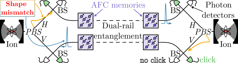
Figure 1: Proposed architecture to connect cavity-coupled ions with two repeater chains, each producing dual-rail entanglement between extreme rare-earth quantum memories (see text for further definitions and explanations).

In this Letter, we tackle this question both at the architecture and physical levels. The architecture we propose uses building blocks that have already been implemented in distinct experiments, see Fig. 1. Two cavity-integrated trapped-ions nodes [16, 17, 18, 19] in distant locations produce telecom photons whose polarization is entangled with the ion energy states [5, 20]. Two repeater chains made with photon pair sources based on spontaneous parametric down conversion (SPDC) and memories based on rare-earth doped crystals [21, 22] are used to distribute dual-rail entanglement [23] between the ions locations. The horizontal (H) and vertical (V) polarizations of photons emitted by the ions are spatially separated by use of polarizing beam splitters (PBS). Each of the two H paths is combined on a beam splitter (BS) with half of a dual-rail entangled state, and similarly for the V paths. A fourfold coincidence detection between photon detectors located after each beam splitter projects the two ions onto an entangled state. This can be seen as an entanglement swapping of ion-photon states mediated by dual-rail entanglement, which results in ion-ion entanglement, see Appendix A. A key condition for the photonic swapping operations to be faithful is that the fields emitted by the ions and the ones released from the rare-earth doped crystals should be indistinguishable in all degrees of freedom. Here, we consider that these two physical platforms produce pure single photons with a temporal mismatch quantified by the square of their waveform overlap, noted $x$, so that the resulting ion-ion fidelity is bounded: $\mathcal{F}_{ion-ion}^{pure}\leq(1+x^{2})/2$, see Appendix A. Fidelities approaching the $0.5$ separability bound are thus expected for state-of-the-art trapped-ion quantum-network node demonstrations, that employ optical cavities for efficient photon collection and achieve photon waveforms that are tens of microseconds long [24], and state-of-the-art rare-earth ensembles, typically storing photons produced by SPDC sources that are a few hundreds of nanoseconds long [21]. While spectral or temporal filtering can be used to restore high fidelities, it comes at the expense of reducing the entanglement distribution rate by $x^{2}$.

The solution that we propose relies on a modification of a commonly used protocol for single-photon storage in rare-earth doped materials [25, 26, 27, 28, 29]—the atomic frequency comb (AFC) protocol [30]. AFC quantum memories are based on a periodic atomic absorption profile in the form of a comb structure, created on an inhomogeneously broadened optical transition using e.g. frequency-selective optical pumping. The absorption of input light pulses whose frequency covers several comb peaks results in echoes after a fixed-delay storage time, which is given by the inverse of the comb period. To extend the storage time and read pulses out on demand, the energy stored in the absorption comb is transferred back and forth to a long-lived state using two $\pi$-pulses. Here, to lengthen the output pulse, we propose partially reading out the energy stored on the long-lived state using a readout pulse weaker than a $\pi$-pulse. Once the light pulse associated with the released energy is emitted, we proceed with another weak readout pulse, resulting in the emission of an additional light pulse. The sequence of weak readouts and light pulse emissions is repeated until all the stored energy is released. We show that this sequential readout technique can be efficient when the crystal is embedded in a cavity which fulfills an impedance matching condition [31, 32, 33]. The technique applies to the quantum regime, where the input light is made of a single photon input, and in this case preserves the photon purity. It allows an arbitrary temporal shaping with a temporal stretching limited only by the coherence time of the long-lived transition (below, inhomogeneous broadening is neglected on the long-lived transition).

The relevance of the proposed protocol is highlighted by a feasibility study in Pr³⁺:Y₂SiO₅ where the photon waveform can be made almost indistinguishable from that of a single ⁴⁰Ca⁺ ion embedded in a high-finesse cavity. Specifically, we show that the visibility of Hong–Ou–Mandel (HOM) [34] interference between the two photons is limited by the purity of ions’ photons for conditions corresponding to a recent experiment with single ⁴⁰Ca⁺ ions [18]. Our results provide a tangible pathway for uniting ⁴⁰Ca⁺ based processors with a quantum repeater backbone using Pr³⁺:Y₂SiO₅ memories [35].

Modeling cavity-assisted AFC –

Each memory is seen as an ensemble of atoms modeled as $\Lambda$ systems; we label the three levels of each system $|g\rangle,$ $|e\rangle$, and $|s\rangle$, see Fig. 2. The optical transition $|g\rangle$-$|e\rangle$ is inhomogeneously broadened, and from a frequency-selective optical pumping, we are left with $N$ atoms whose transition $|g\rangle$-$|e\rangle$ exhibits a periodic comb structure with distribution $n(\omega)$ (period $\Delta$), which is formed of a series of distinct narrow peaks $w(\omega)$ enveloped by a function $v(\omega)$ of total width $\Gamma$. The transition $|g\rangle$-$|s\rangle$ exhibits no inhomogeneous broadening and is considered to feature long-lived coherence. The atoms are embedded into a cavity (amplitude decay rate $\kappa$) which is used to increase the light absorption efficiency of the transition $|g\rangle$-$|e\rangle$ (collective atom-light coupling constant is denoted $g\sqrt{N}$). One of the cavity mirrors is set to couple the single-mode intra-cavity light field to a one dimensional free space mode as described by the input-output formalism [36, 37, 38]. A control field drives the transition $|s\rangle$-$|e\rangle$ with the Rabi frequency $\Omega(t)/2.$ The evolution of the system under an input light pulse to the cavity is given by a set of Heisenberg-Langevin equations [39, 40], see Appendices B and C. Under assumptions that we specify in Appendix D (mainly vacuum Markovian reservoirs and single-photon input), the evolution can equivalently be understood with scalar equations.

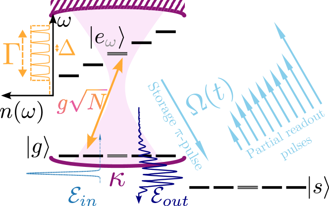
Figure 2: Relevant energy structure for an AFC protocol considered here with a cavity-enhanced efficiency, see Text for the notations. Temporal shaping of the output waveform is obtained by substituting the readout $\pi$-pulse of the standard AFC protocol with a series of weaker partial control pulses with a sufficiently large temporal separation to allow the partial re-emission of the output field.

It is instructive to solve the dynamics by first considering the case without the control field. We show in Appendix B that we can get an explicit expression for the output field (waveform envelope denoted $\mathcal{E}_{out}(t)$) at the first echo time $2\pi/\Delta$ by considering an input single-photon field (waveform envelope labelled $\mathcal{E}_{in}(t)$) with a spectral bandwidth $\delta\omega_{in}$ satisfying $\Gamma,\kappa\gg\delta\omega_{in}>\Delta$,

$$\mathcal{E}_{out}(t\approx\frac{2\pi}{\Delta})\approx-\frac{\tilde{w}(\frac{2\pi}{\Delta})}{\tilde{w}(0)}\frac{4\frac{\mathcal{C}}{\mathcal{C}_{opt}}}{\left(1+\frac{\mathcal{C}}{\mathcal{C}_{opt}}\right)^{2}}\mathcal{E}_{in}(t-\frac{2\pi}{\Delta}).$$ (1)

Specifically, the Fourier transform $\tilde{n}(t)$ of $n(\omega)$ is approximately a comb of peaks $\tilde{v}(t)$ modulated by $\tilde{w}(t)$. $\mathcal{C}=g^{2}N/{\kappa\Gamma}$ is the cooperativity, and $\mathcal{C}_{opt}$ is a constant which depends on $v(\omega)$. For an atomic distribution given by a series of delta functions modulated by a large rectangular envelope, we get $\tilde{w}(\frac{2\pi}{\Delta})\approx\tilde{w}(0)$ and $\mathcal{C}_{opt}=1/\pi$. In this case, Eq. (1) tells us that the overall AFC efficiency $\int_{\frac{2\pi}{\Delta}-\Theta}^{\frac{2\pi}{\Delta}+\Theta}|\mathcal{E}_{out}(t)|^{2}dt/\int_{-\infty}^{+\infty}|\mathcal{E}_{in}(t)|^{2}dt$, with bounds $\Theta$ encompassing only the first AFC echo, is given by $\frac{16\left(\mathcal{C}/\mathcal{C}_{opt}\right)^{2}}{\left(1+\mathcal{C}/\mathcal{C}_{opt}\right)^{4}}.$ It equals $1$ under the impedance matching condition $\mathcal{C}=\mathcal{C}_{opt}$.

We now add the control field into the analysis. When using the control field to implement a pair of $\pi$-pulses with a temporal duration much smaller than $\delta\omega_{in}^{-1}$ for an on-demand storage and readout of the excitation, the relation between the output and input fields is unchanged except for a loss factor $e^{-\gamma_{S}T_{\text{stor}}}$ coming from the decoherence (quantified by a Langevin noise with rate $\gamma_{S}$) during the storage time $T_{\text{stor}}$, i.e., the temporal delay between the two $\pi$-pulses.

Single-photon piecewise pulse shaper based on AFC –

The proposed approach for stretching the output field starts with applying a storage $\pi$-pulse right before the AFC echo. We then use a series of $N_{shape}$ rectangular readout pulses separated by the input-echo time width $\sim$$\delta\omega_{in}^{-1}$, each of which partially transfers the excitation from $|s\rangle$ to $|e\rangle$. The pulses all have a duration $\tau$ much smaller than $\delta\omega_{in}^{-1}$ but distinct areas. The area of pulse $j$ ($1\leq j\leq N_{shape}$) is labelled $r_{j}$ and is such that $\forall j\int\Omega_{j}(t)dt=r_{j}\pi=:2~\mathrm{arcsin}(q_{j})$. When the decoherence on the $|g\rangle$-$|s\rangle$ transition is negligible, we expect that the output field is given by a sequence of bins, all filled by the shape of the input pulse but with an intensity weight given by $p_{j}^{2}=q_{j}^{2}\prod_{k<j}(1-q_{k}^{2})$. If the $r_{j}$ are chosen such that $\sum_{j=1}^{N_{shape}}p_{j}^{2}=1$, and if $\tilde{w}(\frac{2\pi}{\Delta})=\tilde{w}(0)$ and $\mathcal{C}/\mathcal{C}_{opt}=1$, we expect unit overall efficiency of the $N_{shape}$-factor stretching procedure. Refer to Fig. 3 introduced in the next Section for a numerical illustration.

Crucially, we find a recipe to choose the amplitudes and phases of the readout pulses so as to shape the waveform of the output photon and maximize the overlap with any targeted waveform, beyond a simple stretching of the input. In particular, $p_{j}$ is chosen proportional to the overlap between the input translated to bin $j$ and the target restricted to that bin (see Appendix E for more details). This waveform shaping technique preserves photon purity (see Appendix F).

Interestingly, the technique can easily be adapted to preserve the multimode capacity of the AFC protocol, a feature facilitating the realization of quantum repeaters with high entanglement distribution rates [41]. Consider an input field which is a series of time bins, all empty except one that contains a single photon, with the exact temporal location of the photon revealed after the storage $\pi$-pulse. In this case, two synchronisation $\pi$-pulses are added between the storage pulse and the readout pulse series so that the echo of the time bin filled with the photon is emitted immediately after the readout pulses. This avoids unwanted delays between the echos emitted after each readout pulse and preserves the efficiency and versatility of the waveform shaping.

The synchronization pulses turn out to be also useful in the standard case of an input field defined as a single time bin filled with a single photon. They can indeed be used to crop the echos and shorten the temporal separation between the readout pulses. This enhances the overlap with a targeted waveform without much detriment to the efficiency. We call this the cropped-echo technique (see Appendix E).

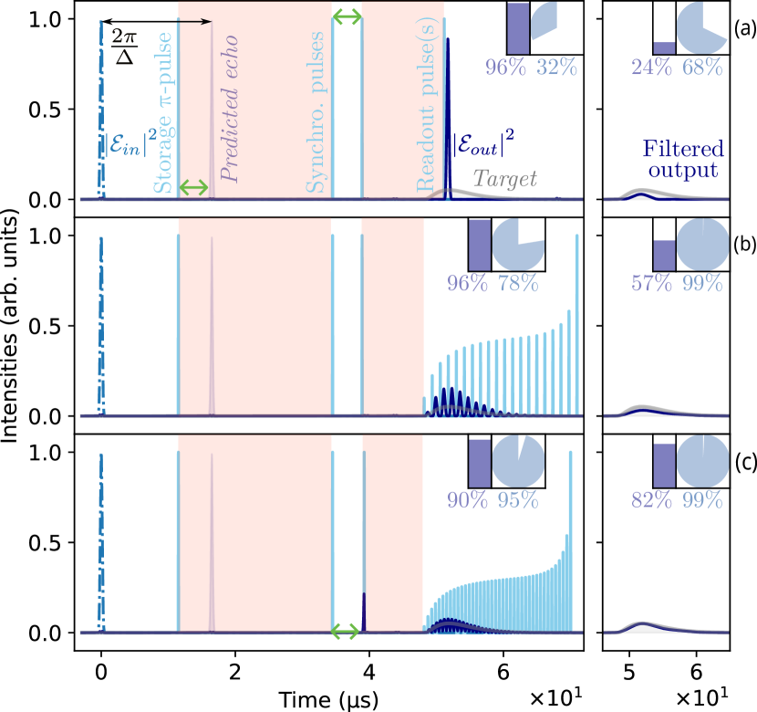
Figure 3: Simulation of cavity-assisted AFC protocols implemented in Pr³⁺:Y₂SiO₅. Left panels show the input field intensity $|\mathcal{E}_{in}(t)|^{2}$ (dash-dotted line), the storage $\pi$-pulse (light blue line) applied before the AFC rephasing time $2\pi/\Delta$ (grayed out), readout pulses (light blue lines), and output field intensity $\left|\mathcal{E}_{out}\right|^{2}$ (dark blue), synchronized and superimposed on a target mode wavefunction (light gray). In the case that the input field occupies an unknown time bin revealed after the storage pulse, two synchonization pulses (light blue lines) are added with a temporal separation (indicated by green double arrows) corresponding to the time delay between the storage pulse and the AFC rephasing time. Input and output intensities are renormalized w.r.t. the input maximal value, while control pulses are renormalized w.r.t. their maximal Rabi frequency. Right panels display filtered output signals, with a sharp cutoff below/above $\pm 2\pi\times 0.15$ MHz. Insets show the AFC efficiency of the output main component (blue rectangular indicators) and the conditional overlap between the output and the target waveform (circular indicators), without and with filtration. The numerical values are also provided. (a) Standard cavity-assisted AFC protocol with a single readout pulse. (b) Waveform shaping with a sequence of readout pulses separated by the echo duration. (c) Cropped-echo readout sequence, where the delay between the synchronization pulses is slightly increased to crop the subsequent echo (see the small output tail before the second synchronization pulse) and the delay between readout pulses is decreased so as to improve overlap with the target.

Numerical results –

For concreteness, we present results of realistic numerical simulations. We focus on a cavity-assisted protocol implemented with a Pr³⁺:Y₂SiO₅ crystal for which an AFC efficiency reaching up to 62% has recently been reported [35]. In particular, the hyperfine transitions $\pm 1/2$ – $\pm 3/2$ and $\pm 3/2$ – $\pm 3/2$ of the ³H₄ – ¹D₂ line are considered for the $|g\rangle$-$|e\rangle$ and $|e\rangle$-$|s\rangle$ transitions respectively. For the AFC, we focus on a rectangular distribution $v$ (width $\Gamma=2\pi\times 4$ MHz) with $67$ Gaussian teeth $w$ (width $\gamma_{tooth}=2\pi\times 1$ kHz), separated by $\Delta=2\pi\times 61$ kHz, and free space mean optical depth $\tilde{d}=0.48$. This choice fulfils the impedance matching condition for a cavity amplitude decay rate $\kappa=2\pi\times 55$ MHz (cavity finesse $\mathcal{F}_{cav}=\pi c/(2L_{cav}\kappa)=6.6$ for cavity length $L_{cav}=208$ mm, mirrors with input and output reflectivity $R_{in}=0.4$ and $R_{out}=1$): $g\sqrt{N}=2\pi\times 8.4$ MHz within the cavity.

We consider a Gaussian input photon with $330$ ns intensity FWHM, and take control pulses almost covering the corresponding $1.3$ MHz photon bandwidth FWHM, hence $\tau=0.07$ µs (from the dipole moment of the optical transition $\pm 3/2$ – $\pm 3/2$, and assuming a beam diameter of $50$ µm, this corresponds to $100$ mW $\pi$-pulse peak power).

The scalar equations discussed above are solved using a numerical integrator, see Appendices G and H for additional details on the parameters and numerical methods. The result is shown in Fig. 3(a), where we observe an overall AFC efficiency of 96% after a $1.6$ µs rephasing time, limited by the AFC (99% absorption) and the $\pi$-pulses bandwidths. We then replace the single readout $\pi$-pulse by $20$ pulses with increasing Rabi frequencies to achieve optimal overlap with a waveform corresponding to the (pure part of a) photon of a cavity-coupled-ion (see below), cf. Fig. 3(b). The efficiency remains unchanged with respect to (w.r.t.) the AFC protocol without pulse shaping but the conditional overlap improves from 32% to 78%. Fig. 3(c) shows that the cropped-echo technique removes detrimental gaps in the piecewise output. The efficiency is almost preserved (90%) and the overlap reaches 95%. Filtering of output photons is also considered in each case to further improve the overlaps with a limited efficiency reduction, see caption of Fig. 3.

Photon waveform matching trapped ion’s emission –

The target waveform was chosen as that of a photon produced by a cavity-coupled ion.

Specifically, we consider a single ⁴⁰Ca⁺ ion, trapped at the waist of an optical cavity, generating single photons via a cavity-mediated Raman transition [42]. We employ here the theoretical model that was used in Ref. [18] to accurately reproduce the photon field observed in their experiments. The photon waveform obtained from this model is asymmetric with a full width half maximum (FWHM) of $\sim$$11$ µs, a fast rising front and longer decreasing tail, see Fig. 4(a). The quality of these photons can be assessed by HOM-like interference, which consists of sending two photons into separate input ports of a beam splitter and recording coincidences on photon detectors placed at the beam splitter outputs (see Appendix I). In the case of perfectly pure and indistinguishable waveforms, the photons bunch, and there is no coincidence detection: the interference visibility reaches $1$. One of the primary sources of imperfections in Ref. [18] was identified as spontaneous emission. Removing spontaneous emission in the simulation leads to pure photons with a FWHM of $\sim$$6$ µs, see Fig. 4 a).

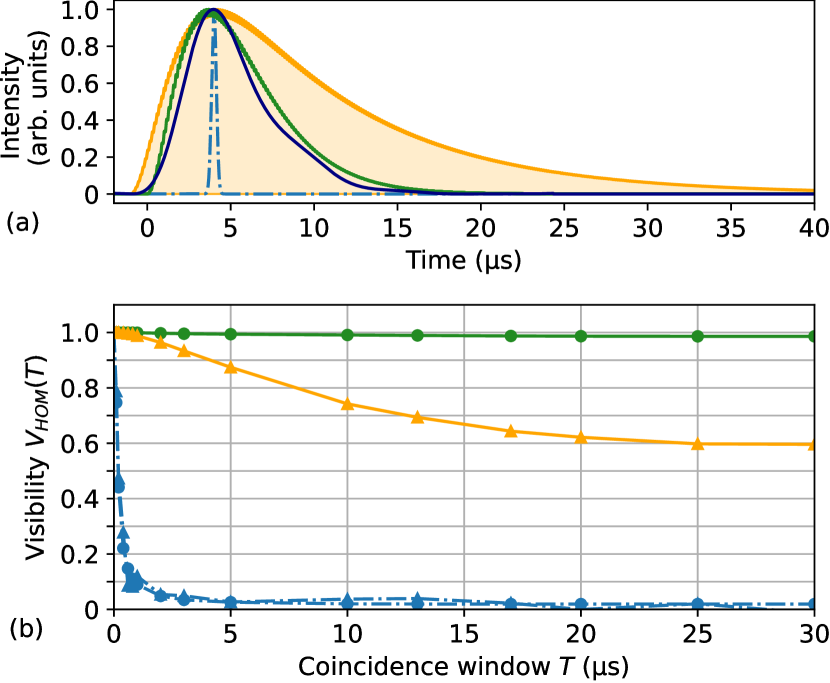
Figure 4: (a) Photon waveform (renormalized field intensities w.r.t. their maximum) emitted by a single ⁴⁰Ca⁺ ion embedded in a cavity [18] (orange) and in the ideal case where unwanted ion spontaneous emission is removed (green). The waveform associated with the photon used as input of the AFC memory (dash-dotted light blue) and the shaped waveform output filtered to discard the arches generated by the shaping (dark blue) are also shown. Synchronization (time offsets) between the waveforms is set to achieve the best possible visibilities. (b) HOM visibility as a function of the acceptance coincidence window between full photons emitted by a single ion and an AFC memory without (blue dash-dotted line with triangles) and with (orange solid line with triangles) waveform shaping. For comparison, the visibilities that would be obtained between a pure ion photon and an AFC photon with (green solid line with bullets) and without shaping (blue dash-dotted line with triangles) are also given.

We are here interested in the HOM interference between a photon emitted by a single ⁴⁰Ca⁺ ion and another coming from an AFC protocol realized in Pr³⁺:Y₂SiO₅. The AFC parameters and the input for the AFC memory are as mentioned above, with the ion-emitted $\sim$$6$ µs–waveform as a shaping target.

The resulting filtered AFC photon waveform is shown in Fig. 4 (a). Fig. 4 (b) shows the interference visibility $V_{HOM}$ as a function of the acceptance coincidence window $T$ without and with the shaping protocol including a filtration of the output photon, as in Fig. 3 right panels. The visibility that would be obtained in the ideal case without spontaneous emission during the ion’s photon emission shows that the visibility in the shaped case is mostly limited by the impurity of the ion’s photon. We add that taking the wider mean waveform as a shaping target did not improve the results.

Conclusion –

We have demonstrated how to expand and shape the waveform of single photons by modifying the AFC protocol, thereby addressing the general problem of how to interface two physical platforms that interact with light on very different timescales. We conclude by quantifying the advantage of this waveform shaping for the long distance entanglement distribution channel shown in Fig. 1. We consider the case where the end memories of the two long-distance repeater chains are each loaded with dual-rail entanglement. As detailed in Appendix A, the probability of getting the four clicks heralding ion-ion entanglement is given by $\mathds{P}_{4cl}=(\eta_{det}^{4}\eta_{mem}^{2}\eta_{ion}^{2})/8$, with $\eta_{det}$ the photon detector efficiency, $\eta_{mem}$ and $\eta_{ion}$ the overall memory and ion efficiencies, which include photon frequency conversion to a shared frequency. The conditional ion-ion state fidelity is given by $\mathcal{F}_{ion-ion}^{mixed}=\frac{1+{V_{HOM}^{\infty}}^{2}}{2}$, where $\infty$ means that we are considering an infinitely large acceptance window $T$ (no post-selection of detection times) and "mixed" refers to the full ion photon. Assuming proven values $\eta_{det}=0.9$, $\eta_{mem}=0.5$ and $\eta_{ion}=0.1$, the basic case without shaping leads to a heralding probability $\mathds{P}_{4cl}=2.2\times 10^{-3}$ and a fidelity $\mathcal{F}_{ion-ion}^{mixed}=0.50$, also achievable with separable states. When the AFC photons are filtered (sharp cutoff of $\pm 2\pi\times 0.15$ MHz) the fidelity increases to $\mathcal{F}_{ion-ion}^{mixed}=0.52$, but the heralding probability is reduced to $\mathds{P}_{4cl}=1.3\times 10^{-4}$. When the AFC photon waveform is shaped and filtered, $\mathds{P}_{4cl}=1.6\times 10^{-3}$ almost reaches the value of the basic case. Moreover, significantly, the fidelity is now well above the separability bound: $\mathcal{F}_{ion-ion}^{mixed}=0.68$. The primary limitation arises from the impurity of the ion-photon state, which could be mitigated by enhancing the cavity cooperativity [43]. Nonetheless, our analysis indicates that entanglement between two ions mediated by rare-earth quantum repeaters is achievable with the current performance parameters.

Acknowledgments –

We thank M. Afzelius, J.-D. Bancal, E. Gouzien, L. Feldmann, S. Grandi, G. Misguich, C. Lanore, P. Sekatski and S. Wengerowsky for insightful discussions. This work received funding from the European Union’s Horizon Europe research and innovation programme under grant agreement No. 101102140 and project name ’QIA-Phase 1’. The opinions expressed in this document reflect only the author’s view and reflect in no way the European Commission’s opinions. The European Commission is not responsible for any use that may be made of the information it contains. P. Cussenot acknowledges funding from the French Direction Générale de l’Armement (DGA).

N.S., H.d.R., T.N., and B.L. proposed the network architecture. P.C., N.S., and A.S. introduced the waveform shaping technique. P.C. and N.S. performed the theoretical analysis with the help of B.G. for the network analysis. P.C. and N.S. wrote the manuscript, with contribution of B.G., and with inputs from all authors. The project was supervised by N.S., B.L., T.N., H.d.R., and A.S..

Appendices: Uniting Quantum Processing Nodes of Cavity-coupled Ions with Rare-earth Quantum Repeaters Using Single-photon Pulse Shaping Based on Atomic Frequency Comb

February 5, 2025

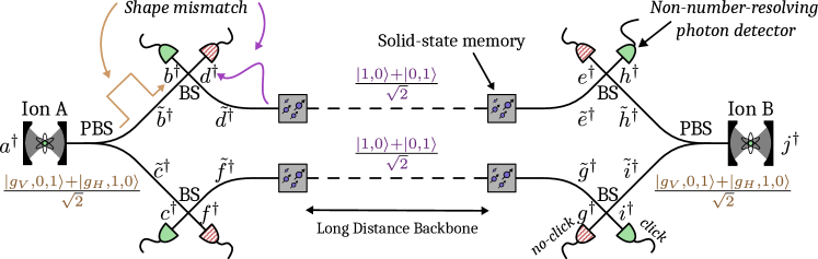
Figure S1: Proposed network architecture, with notations for the different modes involved.

Appendix A Quantum network architecture and fidelity estimation

In this Appendix, we start with an analysis of the quantum network architecture that is given in Fig. 1 of the main text. We explain how entanglement between the two extreme nodes can be generated conditioned on particular detection events and provide explicit formulas for the probability of generation and for the fidelity of the resulting entangled state.

A.1 Presentation of the network protocol

The network architecture is depicted again in Fig. S1. It consists of two long-distance repeater chains [13], each generating entanglement between two solid-state quantum memories; four balanced beam splitters (BS); eight non-photon-number-resolving photodetectors; two polarising beam splitters (PBS); and two ion nodes ($A$ and $B$) [18], thought to be located far apart from one another. In the following analysis, we will assume that the long-distance repeater chains work as ideal entanglement generators. That is, we start with loaded long-distance repeater chains, each producing a pure Bell state $|\Psi^{+}\rangle=\frac{|1,0\rangle+|0,1\rangle}{\sqrt{2}}$, where $|1,0\rangle$ is the state for which the left memory stores an excitation while the right one does not, and conversely for $|0,1\rangle$.

We introduce the vacuum state

$$|\bar{0}\rangle := \quad|g\rangle_{A}\otimes|0\rangle_{\tilde{b}}\otimes|0\rangle_{\tilde{c}}\otimes|0\rangle_{\tilde{d}}\otimes|0\rangle_{\tilde{f}}$$

$$\otimes|0\rangle_{\tilde{e}}\otimes|0\rangle_{\tilde{g}}\otimes|0\rangle_{\tilde{h}}\otimes|0\rangle_{\tilde{i}}\otimes|g\rangle_{B},$$

where letters $(\tilde{b},\tilde{c},\tilde{d},\tilde{e},\tilde{f},\tilde{g},\tilde{h},\tilde{i})$ refer to photon modes of the BS input ports (and PBS output ports). For each of these modes, for instance $\tilde{b}$, the creation of a photon is denoted by $\tilde{b}^{\dagger}|0\rangle_{\tilde{b}}\equiv\tilde{b}^{\dagger}|\bar{0}\rangle$. The driving from state $|g\rangle$ of any of the ions leads to the emission of a photon of polarisation $V$ or $H$, with the ion decaying either in the $|g_{V}\rangle$ or the $|g_{H}\rangle$ state. For convenience, we introduce mode–like operators $a_{H},a_{V}$ and $j_{H},j_{V}$ such that $a_{H}^{\dagger}\left|g\right\rangle_{A}=|g_{H}\rangle_{A}$, $a_{V}^{\dagger}\left|g\right\rangle_{A}=|g_{V}\rangle_{A}$, $j_{H}^{\dagger}\left|g\right\rangle_{B}=|g_{H}\rangle_{B}$, and $j_{V}^{\dagger}\left|g\right\rangle_{B}=|g_{V}\rangle_{B}$.

Initialisation

We start by preparing each ion in a superposition of $|g_{V}\rangle$ and $|g_{H}\rangle$ and collecting the emitted photons, as well as independently loading the repeaters with Bell states and triggering emission from the memories. More precisely, one starts from the state

$$|\psi_{0}\rangle := \quad\left[\frac{a_{H}^{\dagger}\tilde{b}^{\dagger}+a_{V}^{\dagger}\tilde{c}^{\dagger}}{\sqrt{2}}\right]\left[\frac{\tilde{d}^{\dagger}+\tilde{e}^{\dagger}}{\sqrt{2}}\right]$$ (2)

$$\times\left[\frac{\tilde{f}^{\dagger}+\tilde{g}^{\dagger}}{\sqrt{2}}\right]\left[\frac{\tilde{h}^{\dagger}j_{H}^{\dagger}+\tilde{i}^{\dagger}j_{V}^{\dagger}}{\sqrt{2}}\right]|\bar{0}\rangle.$$

As such, the network is loaded with four excitations (photons) in total: one in $\tilde{b}$ or $\tilde{c}$, one in $\tilde{d}$ or $\tilde{e}$, one in $\tilde{f}$ or $\tilde{g}$, and one in $\tilde{h}$ or $\tilde{i}$.

Beam Splitters

The presence of the four beam splitters leads to interference between pairs of modes $(\tilde{b},\tilde{d})$, $(\tilde{c},\tilde{f})$, $(\tilde{h},\tilde{e})$, and $(\tilde{i},\tilde{g})$. For now, we assume that the interference is perfect, so that we introduce modes $(b,d)$, $(c,f)$, $(h,e)$, and $(i,g)$, such that the unitary action of the beam splitters corresponds to the mapping, for instance

$$\begin{cases}\tilde{b}\rightarrow&b=\frac{\tilde{b}+\tilde{d}}{\sqrt{2}}\\ \tilde{d}\rightarrow&d=\frac{\tilde{b}-\tilde{d}}{\sqrt{2}}\end{cases}.$$ (3)

The BS unitary action transforms $|\psi_{0}\rangle$ into

$$|\psi\rangle = \frac{1}{4}\left[a_{H}\cdot\frac{b+d}{\sqrt{2}}+a_{V}\cdot\frac{c+f}{\sqrt{2}}\right]^{\dagger}\left[\frac{b-d}{\sqrt{2}}+\frac{h-e}{\sqrt{2}}\right]^{\dagger}$$

$$\times\left[\frac{c-f}{\sqrt{2}}+\frac{i-g}{\sqrt{2}}\right]^{\dagger}\left[j_{H}\cdot\frac{h+e}{\sqrt{2}}+j_{V}\cdot\frac{i+g}{\sqrt{2}}\right]^{\dagger}|\bar{0}\rangle.$$

Detection and heralding

The heralding step consists of four single-click measurements, one after each beam splitter. Since the network contains exactly four photons delocalised across the optical modes, there are two possible scenarios, depicted in Fig. S2. Clicks on $b$, $c$, $h$, and $i$ leave the ions in $|g_{V}\rangle_{A}\otimes|g_{H}\rangle_{B}$ or in $|g_{H}\rangle_{A}\otimes|g_{V}\rangle_{B}$ depending on whether detector clicks are produced by memories’ or ions’ photons. Due to the lack of which-path information, one ends up with the ion-encoded Bell state

$$|\Psi_{ion-ion}^{+}\rangle=\frac{|g_{V}\rangle_{A}\otimes|g_{H}\rangle_{B}+|g_{H}\rangle_{A}\otimes|g_{V}\rangle_{B}}{\sqrt{2}}.$$ (5)

The case where two photons (here $\tilde{b}$ and $\tilde{d}$) bunch and lead to the same single-click event is discarded by restricting to the heralding of four clicks and not fewer. Note that there are $16$ combinations of detection events with one click after each BS, which lead to the same state 5 up to a local correction (change of the relative phase in the superposition).

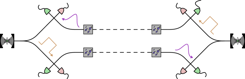
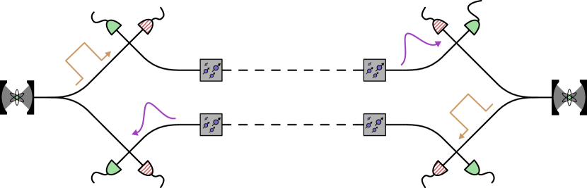
Figure S2: Detection diagrams for four-click scenarios. In the first case, the top-left click comes from the photon being in $\tilde{d}$, which in turn requires the top-right click to stem from a photon in $\tilde{h}$, the bottom-right click from $\tilde{g}$, and the bottom-left from $\tilde{c}$. A possible set of detectors that click is in green, with the other detectors being striped in red.

A.2 Entanglement generation probability and fidelity

We now tackle the network analysis more in depth so as to compute the probability of getting the four clicks and the fidelity of the heralded ion-ion state w.r.t. state 5, in the case where losses happen and devices do not have a unit efficiency. What is more, we now allow the input modes of the beam splitters to represent partially overlapping photon waveforms [44].

A.2.1 Imperfect mode overlap

Indeed, the transformation 3 implicitly assumes that the two incident modes $\tilde{b}$ and $\tilde{d}$ are indistinguishable [45]. In our context, we remind the reader that the photons emitted by the ions and the memories may have different waveforms (see Appendices I and B); this may result in very different spatio-temporal shapes. Following Ref. [46], we will take modes $\tilde{d}$, $\tilde{e}$, $\tilde{f}$, and $\tilde{g}$ as references for each of the beam splitters (modes coming from the memories), and decompose modes (coming from the ions) $\tilde{b}$, $\tilde{h}$, $\tilde{c}$ and $\tilde{i}$ into some interfering components, for which we keep the same notations, and some non-interfering orthogonal components $\tilde{b}_{\perp}$, $\tilde{h}_{\perp}$, $\tilde{c}_{\perp}$, and $\tilde{i}_{\perp}$. For instance, we write

$$\tilde{b}^{\dagger}\rightarrow\sqrt{x_{A}}\tilde{b}^{\dagger}+\sqrt{1-x_{A}}\tilde{b}_{\perp}^{\dagger},$$

where $x_{A}\in[0,1]$ quantifies the degree of waveform overlap (scalar product) with mode $\tilde{d}$ ($x_{A}=1$ when the photons have identical shapes and fully interfere, and $x_{A}=0$ when the modes are orthogonal and do not interfere), with $\langle\bar{0}|\tilde{b}\tilde{b}_{\perp}^{\dagger}|\bar{0}\rangle=\langle\bar{0}|[\tilde{b},\tilde{b}_{\perp}^{\dagger}]|\bar{0}\rangle=0$. For simplicity, we take a symmetric situation where the value of $x_{A}$ is the same for the overlaps ($\tilde{b},\tilde{d}$) and ($\tilde{c},\tilde{f}$), while $x_{B}$ is defined for the overlaps ($\tilde{e},\tilde{h}$) and ($\tilde{g},\tilde{i}$). Then the unitary transformation due to the beam splitters acts independently on orthogonal modes, so that the state A.1 before detection is now given by

(6)

$$|\psi\rangle= \frac{1}{4}\left[\sqrt{x_{A}}\left(a_{H}\cdot\frac{b+d}{\sqrt{2}}+a_{V}\cdot\frac{c+f}{\sqrt{2}}\right)+\sqrt{1-x_{A}}\left(a_{H}\cdot\frac{b_{\perp}+d_{\perp}}{\sqrt{2}}+a_{V}\cdot\frac{c_{\perp}+f_{\perp}}{\sqrt{2}}\right)\right]^{\dagger}\times\left[\frac{b-d}{\sqrt{2}}+\frac{h-e}{\sqrt{2}}\right]^{\dagger}$$

$$\times\left[\frac{c-f}{\sqrt{2}}+\frac{i-g}{\sqrt{2}}\right]^{\dagger}\times\left[\sqrt{x_{B}}\left(j_{H}\cdot\frac{h+e}{\sqrt{2}}+j_{V}\cdot\frac{i+g}{\sqrt{2}}\right)+\sqrt{1-x_{B}}\left(j_{H}\cdot\frac{h_{\perp}+e_{\perp}}{\sqrt{2}}+j_{V}\cdot\frac{i_{\perp}+g_{\perp}}{\sqrt{2}}\right)\right]^{\dagger}|\underline{0}\rangle,$$

where we introduced $d_{\perp}$, $e_{\perp}$, $f_{\perp}$, and $g_{\perp}$ (as well as $b_{\perp}$, $h_{\perp}$, $c_{\perp}$, and $i_{\perp}$without the tilde superscript) as the orthogonal output modes after the beam splitters (for orthogonal input modes, the BS relation is for instance given by $\tilde{b}_{\perp}\rightarrow\frac{b_{\perp}+d_{\perp}}{\sqrt{2}}$, and no input of the type $\tilde{d}_{\perp}$ is to be considered).

A.2.2 Detection POVMs

We then build the Positive Operator-Valued Measure operator (POVM) associated to the non-photon-resolving photodetectors. If one provides an orthogonal mode basis [44] for the light arriving on detector $b$, that we note as a set of $\beta_{k}$ with mode index $k$, then the POVM for a no-click event on $b$ is defined as

$$\Pi_{nc}^{b}:=(1-\eta_{det})^{\sum_{k}\beta_{k}^{\dagger}\beta_{k}}=\prod_{k}(1-\eta_{det})^{\beta_{k}^{\dagger}\beta_{k}},$$ (7)

where $\eta_{det}$ is the efficiency of the detector and $[\beta_{k},\beta_{k^{\prime}\neq k}]=0$, $[\beta_{k},\beta_{k^{\prime}\neq k}^{\dagger}]=0$. Using the Baker-Campbell-Hausdorff formula, one can see that $\Pi_{nc}^{b}$ is diagonal in the Fock basis for modes $\beta_{k}$, and the probability of not detecting a number state with $M_{k}$ photons in the mode $\beta_{k}$ is $\frac{1}{M_{k}!}\langle 0|\beta_{k}^{M_{k}}\Pi_{nc}^{b}(\beta_{k}^{M_{k}})^{\dagger}|0\rangle=(1-\eta_{det})^{M_{k}}$. In particular, $\langle 0|\Pi_{nc}^{b}|0\rangle=1$. Then if we decompose the output $b$ into the basis $\{\beta_{k}\}_{k}$ by writing $b^{\dagger}=\sum_{k}\gamma_{k}\beta_{k}^{\dagger}$, we note that

$$\Pi_{nc}^{b}b^{\dagger}|0\rangle =(1-\eta_{det})^{\sum_{k}\beta_{k}^{\dagger}\beta_{k}}b^{\dagger}|0\rangle$$

$$=(1-\eta_{det})^{\sum_{k}\beta_{k}^{\dagger}\beta_{k}}\left(\sum_{k}\gamma_{k}\beta_{k}^{\dagger}\right)|0\rangle$$

$$=\sum_{k}\gamma_{k}\cdot(1-\eta_{det})\beta_{k}^{\dagger}|0\rangle$$

$$=(1-\eta_{det})b^{\dagger}|0\rangle.$$

An identical derivation leads to $\Pi_{nc}^{b}b_{\perp}^{\dagger}|0\rangle=(1-\eta_{det})b_{\perp}^{\dagger}|0\rangle$. This shows that $\Pi_{nc}^{b}$ is a suitable POVM for the non-click event at the detector whatever the incoming mode (like $b$, $b_{\perp}$ and others). Similarly, the complementary POVM for a click event is introduced as

$$\Pi_{c}^{b}=\mathds{1}-\Pi_{nc}^{b}=\mathds{1}-(1-\eta_{det})^{\sum_{k}\beta_{k}^{\dagger}\beta_{k}}.$$

Note that

$$\Pi_{c}^{b}|0\rangle = |0\rangle-|0\rangle=0$$

$$\Pi_{c}^{b}b_{\perp}^{\dagger}|0\rangle = b_{\perp}^{\dagger}\Pi_{c}^{b}|0\rangle=0.$$ (8)

Likewise, POVMs $\Pi_{nc}^{d}$, $\Pi_{c}^{d}$, $\Pi_{nc}^{c}$, $\Pi_{c}^{c}$, $\Pi_{nc}^{f}$, $\Pi_{c}^{f}$, $\Pi_{nc}^{e}$, $\Pi_{c}^{e}$, $\Pi_{nc}^{h}$, $\Pi_{c}^{h}$, $\Pi_{nc}^{g}$, $\Pi_{c}^{g}$, $\Pi_{nc}^{i}$, $\Pi_{c}^{i}$ are introduced for the other photodetectors.

A.2.3 Four-click event

There are $2^{4}=16$ ways for exactly one detector per beam splitter pair to click simultaneously as a four-click event that we look for. For clarity, we focus on one way, which corresponds to the situation on the top of Fig. S2 (detectors that click are in green, namely $b$, $c$, $h$, and $i$). For this situation, the four-click event POVM is given by

$$\Pi_{4cl,1}=(\Pi_{c}^{b}\times\Pi_{nc}^{d})\times(\Pi_{c}^{c}\times\Pi_{nc}^{f})\times(\Pi_{c}^{h}\times\Pi_{nc}^{e})\times(\Pi_{c}^{i}\times\Pi_{nc}^{g}),$$

where all factors commute with one another. Starting from Eq. 6, the heralded state after detection is then

$$\rho_{ion-ion}=\frac{1}{\mathds{P}_{4cl,1}}\mathrm{Tr}_{repeaters}\left(\Pi_{4c,1}|\psi\rangle\langle\psi|\right),$$

where $\mathrm{Tr}_{repeaters}$ denotes the partial trace over the inner modes (i.e., all modes but $a$ and $j$), and the normalisation constant

$$\mathds{P}_{4cl,1}=\mathrm{Tr}\left(\Pi_{4c,1}|\Psi\rangle\langle\Psi|\right)$$

is the heralding probability of that specific four-click event.

Expanding the expression of $\Pi_{4c,1}|\Psi\rangle\langle\Psi|$ yields many zero terms: the only non-zero terms are those for which the detection modes ($b$, $c$, $h$, and $i$ or their orthogonal counterparts) are loaded with four excitations in $|\Psi\rangle$ (see Eq. 8, and recall that $\Pi_{c}^{b}$ is a click due to a photon arriving either through $b$ or through $b_{\perp}$). Typically, $\Pi_{4c,1}b^{\dagger}c^{\dagger}h_{\perp}^{\dagger}i^{\dagger}|\bar{0}\rangle=\eta_{det}^{4}b^{\dagger}c^{\dagger}h^{\dagger}i^{\dagger}|\bar{0}\rangle$ but $\Pi_{4c,1}a_{V}^{\dagger}c_{\perp}^{\dagger}b^{\dagger}f^{\dagger}i_{\perp}^{\dagger}j_{V}^{\dagger}|\bar{0}\rangle=0$. Picking relevant creation operators yields $8$ non-zero terms only, which are provided in Table 1 together with the related coefficient in the expansion of $|\psi\rangle$ and the state $|g_{H}\rangle$ or $|g_{V}\rangle$ to which the ions decayed. The expansion is also weighted by a $\eta_{det}^{4}$ coefficient, corresponding to the success probability of $4$ detections.

	1 factor	2 factor	3 factor	4 factor	Coefficient	Ion modes involved
Among	$b,c,b_{\perp},c_{\perp}$	$b,h$	$c,i$	$h,i,h_{b},i_{\perp}$
	$b$	$h$	$c$	$i$	$\frac{1}{16}\cdot\sqrt{x_{A}x_{B}}$	$a_{H}$ and $j_{V}$
	$b$	$h$	$c$	$i_{\perp}$	$\frac{1}{16}\cdot\sqrt{x_{A}}\cdot\sqrt{1-x_{B}}$
	$b_{\perp}$	$h$	$c$	$i$	$\frac{1}{16}\cdot\sqrt{1-x_{A}}\cdot\sqrt{x_{B}}$
	$b_{\perp}$	$h$	$c$	$i_{\perp}$	$\frac{1}{16}\cdot\sqrt{1-x_{A}}\sqrt{1-x_{B}}$
	$c$	$b$	$i$	$h$	$\frac{1}{16}\cdot\sqrt{x_{A}x_{B}}$	$a_{V}$ and $j_{H}$
	$c$	$b$	$i$	$h_{\perp}$	$\frac{1}{16}\cdot\sqrt{x_{A}}\cdot\sqrt{1-x_{B}}$
	$c_{\perp}$	$b$	$i$	$h$	$\frac{1}{16}\cdot\sqrt{1-x_{A}}\cdot\sqrt{x_{B}}$
	$c_{\perp}$	$b$	$i$	$h_{\perp}$	$\frac{1}{16}\cdot\sqrt{1-x_{A}}\sqrt{1-x_{B}}$

Table 1: Summary of all the 8 combinations built from the modes $b,c,h,i$ or their respective orthogonal modes, representing the non-zero terms of $\Pi_{4c,1}|\Psi\rangle$. Note that the first and the fifth combinations involve the same inner network nodes $b,h,c,i$.

Taking the partial trace w.r.t. all mode operators except $a_{H}$, $a_{V}$, $j_{H}$, and $j_{V}$ yields the decomposition

$$\mathrm{Tr}_{repeaters}\left(\Pi_{4c,1}|\psi\rangle\langle\psi|\right)= \eta_{det}^{4} \left[\frac{x_{A}x_{B}}{256}|\Psi_{ion-ion}^{+}\rangle\langle\Psi_{ion-ion}^{+}|\right.$$

$$+\left(\frac{x_{A}(1-x_{B})}{256}+\frac{(1-x_{A})x_{B}}{256}+\frac{(1-x_{A})(1-x_{B})}{256}\right)|g_{H}\rangle_{A}\otimes|g_{V}\rangle_{B}\langle g_{H}|_{A}\otimes\langle g_{V}|_{B}$$

$$\left.+\left(\frac{x_{A}(1-x_{B})}{256}+\frac{(1-x_{A})x_{B}}{256}+\frac{(1-x_{A})(1-x_{B})}{256}\right)|g_{V}\rangle_{A}\otimes|g_{H}\rangle_{B}\langle g_{V}|_{A}\otimes\langle g_{H}|_{B}\right]$$

$$= \eta_{det}^{4} \left[\frac{1}{256}|g_{V}\rangle_{A}\otimes|g_{H}\rangle_{B}\langle g_{V}|_{A}\otimes\langle g_{H}|_{B}+|g_{H}\rangle_{A}\otimes|g_{V}\rangle_{B}\langle g_{H}|_{A}\otimes\langle g_{V}|_{B}\right.$$

$$\left.+\frac{x_{A}x_{B}}{256}|g_{V}\rangle_{A}\otimes|g_{H}\rangle_{B}\langle g_{H}|_{A}\otimes\langle g_{V}|_{B}+|g_{H}\rangle_{A}\otimes|g_{V}\rangle_{B}\langle g_{V}|_{A}\otimes\langle g_{H}|_{B}\right].$$

The four-click probability of our particular event is

$$\mathds{P}_{4cl,1}=\frac{\eta_{det}^{4}}{128},$$

and we finally obtain the density matrix

$$\rho_{ion-ion}= \frac{1}{2}\left(1+x_{A}x_{B}\right)|\Psi_{ion-ion}^{+}\rangle\langle\Psi_{ion-ion}^{+}|$$

$$+ \frac{1}{2}\left(1-x_{A}x_{B}\right)|\Psi_{ion-ion}^{+}\rangle\langle\Psi_{ion-ion}^{+}|.$$

The fidelity w.r.t. the expected target state $|\Psi_{ion-ion}^{+}\rangle$ (see Eq. 5) is thus

$$\mathcal{F}_{ion-ion}=\frac{1}{2}\left(1+x_{A}x_{B}\right).$$ (10)

Furthermore, the total four-click probability is

$$\mathds{P}_{4cl}=16\times\mathds{P}_{4cl,1}=\frac{\eta_{det}^{4}}{8},$$ (11)

which is not suprising since $2$ out of $16$ path combinations for the four excitations lead to a four-click event.

A.2.4 Imperfect situation

So far, we assumed a perfect situation where both the memories and the ions emit photons with unit efficiency, and no propagation loss occur. We can now introduce $\eta_{ion}$ and $\eta_{rep}$ as the efficiencies, including fiber losses, for the ions and solid-state memories (assumed symmetric for the left and right sides of the network architecture). Tracing out the loss channels leads to the initialised state $\rho_{0}=\begin{aligned} \rho_{ion}^{A}\end{aligned}\otimes\rho_{rep}^{up}\otimes\rho_{rep}^{down}\otimes\begin{aligned} \rho_{ion}^{B}\end{aligned}$, with

$$\begin{aligned} \rho_{ion}^{A}\end{aligned} = \quad\left(1-\eta_{ion}\right)|0\rangle\langle 0|$$

$$+\eta_{ion}\left[\frac{a_{H}^{\dagger}\tilde{b}^{\dagger}+a_{V}^{\dagger}\tilde{c}^{\dagger}}{\sqrt{2}}\right]|0\rangle\langle 0|\left[\frac{a_{H}\tilde{b}+a_{V}\tilde{c}}{\sqrt{2}}\right],$$

$$\rho_{rep}^{up} = \quad\left(1-\eta_{rep}\right)|0\rangle\langle 0|$$

$$+\eta_{rep}\left[\frac{\tilde{d}^{\dagger}+\tilde{e}^{\dagger}}{\sqrt{2}}\right]|0\rangle\langle 0|\left[\frac{\tilde{d}+\tilde{e}}{\sqrt{2}}\right],$$

$$\rho_{rep}^{down} = \quad\left(1-\eta_{rep}\right)|0\rangle\langle 0|$$

$$+\eta_{rep}\left[\frac{\tilde{f}^{\dagger}+\tilde{g}^{\dagger}}{\sqrt{2}}\right]|0\rangle\langle 0|\left[\frac{\tilde{f}+\tilde{g}}{\sqrt{2}}\right],$$

$$\begin{aligned} \rho_{ion}^{B}\end{aligned} = \quad\left(1-\eta_{ion}\right)|0\rangle\langle 0|$$

$$+\eta_{ion}\left[\frac{\tilde{h}^{\dagger}j_{H}^{\dagger}+\tilde{i}^{\dagger}j_{V}^{\dagger}}{\sqrt{2}}\right]|0\rangle\langle 0|\left[\frac{\tilde{h}j_{H}+\tilde{i}j_{V}}{\sqrt{2}}\right].$$

Using previous derivations to identify the relevant four-excitation components after the beam splitters’ unitary action leads to the total four-click probability

$$\mathds{P}_{4cl}=\frac{\eta_{\text{det}}^{4}\eta_{\text{ion}}^{2}\eta_{\text{rep}}^{2}}{8},$$

which is not surprising since a four-click event requires $2$ photons coming from the ions and $2$ photons coming from the memories. The heralded state and its fidelity are unaffected.

A.3 Mixture

We then point out that the initial ion-photon states may not be pure for realistic experiments. As detailed in Appendix I (which focuses on experiments [24, 47]), the initial ion-photon state is rather described by a continuous mixture of pure components that we write here

$$\begin{aligned} \rho_{ion}^{A}\end{aligned}=\left(1-\eta_{ion}\right)|0\rangle\langle 0|+\int\bar{P}_{A}(s)\left[\frac{a_{H}^{\dagger}\tilde{b}^{\dagger}(s)+a_{V}^{\dagger}\tilde{c}^{\dagger}(s)}{\sqrt{2}}\right]|0\rangle\langle 0|\left[\frac{a_{H}\tilde{b}(s)+a_{V}\tilde{c}(s)}{\sqrt{2}}\right]\mathrm{ds}$$

with a probability distribution $\bar{P}_{A}(s)$ such that $\int\bar{P}_{A}(s)\mathrm{d}s=\eta_{ion}$ and a collection of optical modes $\{\tilde{b}(s),\tilde{c}(s)\}$ (not orthogonal to one another) that depend on the value of $s$ (while the related ion state is supposed independent of $s$). A similar state $\rho_{ion}^{B}$ is introduced with a distribution $\bar{P}_{B}(s)$ and modes $\{\tilde{h}(s),\tilde{i}(s)\}$.

The linearity of the equations (that crucially relies on the fact that we introduced some detection POVMs that are independent of the incoming modes) then leads to the heralded state fidelity w.r.t. the Bell state

$$\mathcal{F}_{ion-ion}^{mixed}=\frac{1}{2}\left(1+\int\bar{P}_{A}(s)x_{A}(s)\mathrm{ds}\int\bar{P}_{B}(s^{\prime})x_{B}(s^{\prime})\mathrm{ds^{\prime}}\right),$$ (12)

where $x_{A}(s)$ ($x_{B}(s)$) is the overlap between the modes $\tilde{b}(s)$ or $\tilde{c}(s)$ ($\tilde{h}(s)$ or $\tilde{i}(s)$) and the mode $\tilde{d}$ or $\tilde{f}$ ($\tilde{e}$ or $\tilde{g}$). The total four-click probability is kept unchanged:

$$\mathds{P}_{4cl}=\frac{\eta_{\text{det}}^{4}\int\bar{P}_{A}(s)\mathrm{d}s\int\bar{P}_{B}(s)\mathrm{d}s\eta_{\text{rep}}^{2}}{8}=\frac{\eta_{\text{det}}^{4}\eta_{\text{ion}}^{2}\eta_{\text{rep}}^{2}}{8}.$$ (13)

In Appendix I, we will show that the fidelities 10 and 12 can be related to the visibilities of Hong Ou Mandel–like experiments between the photons of the memories and of the ions (see Eqs. I.2.2, 188, 189, and 190).

Furthermore, we point out that a clear way to enhance the heralded state fidelity is to increase the overlap between the memory photon mode and at least one ion photon mode. However, this enhancement in overlap should not be too detrimental to the emission efficiencies and thus the value of entanglement generation rate of the repeater. This is the goal of our shaping protocol, which we will detail in Appendix E. Numerical estimations of the overlaps are provided.

A.4 Experimental efficiencies

Finally, we provide experimentally relevant values for the efficiencies $\eta_{det}$, $\eta_{ion}$ and $\eta_{mem}$. For the memory emission, we write $\eta_{mem}=\eta_{AFC,shaping}\times\eta_{QFC}$ where we include the efficiency of the AFC shaping process $\eta_{AFC,shaping}$, which we take to be $82$ % (see main text), and some end-to-end conversion to telecom wavelength with efficiency $\eta_{QFC}=60$ % based on Refs. [48, 49]. For the ions’ emission, we assume an overall efficiency $\eta_{ion}=10$ % including the wavelength conversion [50]. For non-photon-number-resolving photodetectors, we take $\eta_{det}=90$ %.

Note that the repeaters might start with some infidelity w.r.t. the Bell states involved in state 2, which would result in the heralded fidelities being only bounded from above by the values given in 10 and 12.

Appendix B Modelling a cavity-assisted AFC quantum memory

In this Appendix, we build upon previous derivations from the literature to provide an extended presentation of a model of an AFC quantum memory at the single photon level. The conventions chosen for the different parameters as compared with other articles, and suggested experimental values extracted from the literature will be provided in Appendix G.

B.1 Inhomogeneous ensemble of $\Lambda$-systems

We first set out the physical model of a cavity-assisted AFC quantum memory, which consists of a collection of doping ions embedded in a crystal structure within an optical cavity [31, 32]. We model it as an inhomogeneously broadened ensemble of $\Lambda$-systems interacting with a single cavity mode which is coupled to input and output fields in the environment. We build the equations for quantum operators involved in the description of the full $\Lambda$-structure, and then obtain a set of scalar equations.

B.1.1 Set of equations for quantum operators

The system of interest comprises a cavity, an assembly of $N$ atoms, a collection of modes of the environment that will collect input and output light, and the rest of the environment, made of different baths.

Hamiltonian part of the equations

The Hamiltonian Hilbert space is initially defined as the tensor product of all Hilbert spaces introduced to describe individual components of the system (without the environment in a first place), as

$$\mathcal{H}_{mem} = \mathcal{H}_{cav}\otimes\bigotimes_{j=1}^{N}\mathcal{H}_{j}.$$ (14)

To represent the interactions between all the components, we follow Refs. [51, 39] and introduce the simplified Hamiltonian

$$\hat{H} = \hat{H}_{cav}+\hat{H}_{at}+\hat{H}_{int}+\hat{H}_{trans},$$ (15)

with

$$\hat{H}_{cav} = \hbar\omega_{c}\hat{a}^{\dagger}\hat{a},$$

$$\hat{H}_{at} = \hbar\sum_{k}\left(\Delta_{k}\hat{\sigma}_{ee}^{(k)}-\omega_{s}\hat{\sigma}_{ss}^{(k)}\right),$$

$$\hat{H}_{int} = -\hbar g\sum_{k}\left(\hat{a}\hat{\sigma}_{eg}^{(k)}+\hat{a}^{\dagger}\hat{\sigma}_{ge}^{(k)}\right),$$

$$\hat{H}_{trans} = -\frac{\hbar}{2}\sum_{k}\left(\Omega(t)e^{-i\omega_{r}t}\hat{\sigma}_{es}^{(k)}+\Omega^{*}(t)e^{+i\omega_{r}t}\hat{\sigma}_{se}^{(k)}\right).$$

In this Hamiltonian, $\hat{H}_{cav}$ and $\hat{H}_{at}$ describe the free evolution of a single mode of the cavity field and the atoms, $\hat{H}_{int}$ models the interaction between the cavity mode and the atoms in a two-level approximation, and $\hat{H}_{trans}$ is the semi-classical Rabi Hamiltonian for the driving of the third levels by a strong classical pulse.

Furthermore,

• $\hat{a}$ is the annihilation operator for the mode (frequency $\omega_{c}$) of interest of the electric field inside the cavity at the position where the atoms are considered, namely $\hat{\boldsymbol{E}}(t)=\boldsymbol{\epsilon}\sqrt{\frac{\hbar\omega_{c}}{2\varepsilon_{0}V}}\left[\hat{a}(t)+\hat{a}^{\dagger}(t)\right]$. Recall that, in the free field evolution only, $\hat{a}(t)=e^{-i\omega_{c}t}\hat{a}(0)$ due to Hamiltonian evolution under $\hbar\omega_{c}\hat{a}^{\dagger}\hat{a}$: the exponential term then gives the oscillations of the field in the Heisenberg picture. The polarisation unit vector $\boldsymbol{\epsilon}$ is chosen so as to correctly address the atomic $|g\rangle\rightarrow|e\rangle$ transition under angular momentum conservation. $V$ is the quantisation volume for the cavity mode, typically

  $$V=AL_{cav}$$ (16)

  with $A$ the mode cross section and $L_{cav}$ the length of the cavity. The operator $\hat{a}$ abides by the commutation relation

  $$[\hat{a}(0),\hat{a}^{\dagger}(0)]=\mathds{I},$$ (17)

  which is conserved for any unitary evolution.

• $k$ indices in summations refer to different atomic frequency classes. In each class, $N_{k}$ atoms share the same $|g\rangle\rightarrow|e\rangle$ transition frequency $\Delta_{k}$. It is assumed that all classes share the same $|g\rangle\rightarrow|s\rangle$ transition frequency $\omega_{s}$, which does not depend on $k$. For every class, a collective coherence operator is introduced as the sum of atomic coherences:

  • $\hat{\sigma}_{eg}^{(k)}:=\sum_{j=1}^{N_{k}}|e\rangle_{jj}\langle g|=\left(\hat{\sigma}_{ge}^{(k)}\right)^{\dagger}$ is the internal state operator for the $|g\rangle\rightarrow|e\rangle$ optical transition of atomic class $k$;

  • $\hat{\sigma}_{sg}^{(k)}:=\sum_{j=1}^{N_{k}}|s\rangle_{jj}\langle g|=\left(\hat{\sigma}_{gs}^{(k)}\right)^{\dagger}$ is the internal state operator for the $|g\rangle\rightarrow|s\rangle$ spin transition of atomic class $k$;

  • More generally, $\hat{\sigma}_{\alpha\beta}^{(k)}:=\sum_{j=1}^{N_{k}}|\alpha\rangle_{jj}\langle\beta|=\left(\hat{\sigma}_{\beta\alpha}^{(k)}\right)^{\dagger}$ refers to the internal state operator for the $|\alpha\rangle\rightarrow|\beta\rangle$ level transition of atomic class $k$. When $\alpha=\beta$, $\hat{\sigma}_{\alpha\alpha}$ refers to the population of energy level $\alpha$ so that for all $k$ $\hat{\sigma}_{gg}^{(k)}+\hat{\sigma}_{ee}^{(k)}+\hat{\sigma}_{ss}^{(k)}=N_{k}\mathds{1}_{\mathcal{H}_{k}}$. In addition, one can check that the collective operators keep similar commutation relations, namely $\left[\hat{\sigma}_{\alpha\beta}^{(k)}(0),\hat{\sigma}_{\mu\nu}^{(j)}(0)\right]=\delta_{kj}\left(\delta_{\beta\mu}\hat{\sigma}_{\alpha\nu}^{(k)}(0)-\delta_{\nu\alpha}\hat{\sigma}_{\mu\beta}^{(k)}(0)\right)$, which are conserved throughout any unitary evolution ($\delta_{\alpha\beta}$ are Kronecker deltas here);

  • The total number of atoms in the system is $N:=\sum_{k}N_{k}$, and for every $k$ we define

    $$n_{k}:=\frac{N_{k}}{N}$$ (18)

    the density of atoms with frequency class $k$ ($\sum_{k}n_{k}=1$);

  • Typically, $N$ is much bigger than the number of excitations in the system, namely $N\gg 1$, so that one can introduce the low population hypothesis (see 7 below).

• $g$ is the coupling constant between the cavity mode field and the atoms for the $|g\rangle\rightarrow|e\rangle$ optical transition, assumed to be homogeneous accross classes. Working with the dipole approximation, we set $\hat{\boldsymbol{d}}_{j}=\langle g|_{j}\hat{\boldsymbol{d}}_{j}|e\rangle_{j}|g\rangle_{jj}\langle e|+\langle e|_{j}\hat{\boldsymbol{d}}_{j}|g\rangle_{j}|e\rangle_{jj}\langle g|=\langle g|_{j}\hat{\boldsymbol{d}}_{j}|e\rangle_{j}\left[|g\rangle_{jj}\langle e|+\left(|g\rangle_{jj}\langle e|\right)^{\dagger}\right]$ for the dipole moment vector operator of atom $j$, with a convenient phase so that the conjugated matrix elements appear real. Then the dipole-field interaction for the $|g\rangle\rightarrow|e\rangle$ transition is given by $-\hat{\boldsymbol{d}}_{j}\cdot\hat{\boldsymbol{E}}=-\langle g|_{j}\hat{\boldsymbol{d}}_{j}\cdot\boldsymbol{\epsilon}|e\rangle_{j}\sqrt{\frac{\hbar\omega_{c}}{2\varepsilon_{0}V}}\left[|g\rangle_{jj}\langle e|+\left(|g\rangle_{jj}\langle e|\right)^{\dagger}\right]\left[\hat{a}+\hat{a}^{\dagger}\right]$. With the rotating-wave approximation (RWA), terms involving $|g\rangle_{jj}\langle e|\hat{a}$ and $\left(|g\rangle_{jj}\langle e|\right)^{\dagger}\hat{a}^{\dagger}$ are discarded. We obtain $-\hat{\boldsymbol{d}}_{j}\cdot\hat{\boldsymbol{E}}\approx-\langle g|_{j}\hat{\boldsymbol{d}}_{j}\cdot\boldsymbol{\epsilon}|e\rangle_{j}\sqrt{\frac{\hbar\omega_{c}}{2\varepsilon_{0}V}}\left[|g\rangle_{jj}\langle e|\hat{a}^{\dagger}+\left(|g\rangle_{jj}\langle e|\right)^{\dagger}\hat{a}\right]=:-\hbar g\left[|g\rangle_{jj}\langle e|\hat{a}^{\dagger}+\left(|g\rangle_{jj}\langle e|\right)^{\dagger}\hat{a}\right]$ where we take (approximately for any $j$)

  $$g:=\langle g|_{j}\hat{\boldsymbol{d}}_{j}\cdot\boldsymbol{\epsilon}|e\rangle_{j}\sqrt{\frac{\omega_{c}}{2\hbar\varepsilon_{0}V}}.$$ (19)

• $\Omega$ is the Rabi frequency of the driving field for the $|s\rangle\rightarrow|e\rangle$ transition. For this, we introduce the classical driving field of frequency $\omega_{r}$, $\boldsymbol{E}_{r}(t)=\boldsymbol{\epsilon}_{r}\frac{\left[E_{r}(t)e^{-i\omega_{r}t}+E_{r}^{*}(t)e^{+i\omega_{r}t}\right]}{2}$ , where $E_{r}(t)$ gives the slowly-varying modulation shape of the driving pulse (typically chosen real and rectangular-shaped in the following) and $\boldsymbol{\epsilon}_{r}$ is the polarisation unit vector. With the rotating-wave and dipole approximations, we introduce the dipole moment vector $\hat{\boldsymbol{b}}_{j}=\langle s|_{j}\hat{\boldsymbol{b}}_{j}|e\rangle_{j}|s\rangle_{jj}\langle e|+\langle e|_{j}\hat{\boldsymbol{b}}_{j}|s\rangle_{j}|e\rangle_{jj}\langle s|=\langle s|_{j}\hat{\boldsymbol{b}}_{j}|e\rangle_{j}\left[|s\rangle_{jj}\langle e|+\left(|s\rangle_{jj}\langle e|\right)^{\dagger}\right]$, and the dipole-field interation for the $|s\rangle\rightarrow|e\rangle$ transition is given by $-\hat{\boldsymbol{b}}_{j}\cdot\boldsymbol{E}_{r}\approx-\frac{\langle s|_{j}\hat{\boldsymbol{b}}_{j}\cdot\boldsymbol{\epsilon}_{r}|e\rangle_{j}}{2}\left[E_{r}^{*}(t)e^{+i\omega_{r}t}|s\rangle_{jj}\langle e|+h.c.\right]=:-\frac{\hbar}{2}\left[\Omega^{*}(t)e^{+i\omega_{r}t}|s\rangle_{jj}\langle e|+\Omega(t)e^{-i\omega_{r}t}\left(|s\rangle_{jj}\langle e|\right)^{\dagger}\right]$ with for any $j$

  $$\Omega(t)=\frac{1}{\hbar}\langle g|_{j}\hat{\boldsymbol{b}}_{j}\cdot\boldsymbol{\epsilon}_{r}|s\rangle_{j}E_{r}(t).$$ (20)

  Contrary to Ref. [40], we do not include any factor $2$ into the definition of $\Omega$ so that a factor $\frac{1}{2}$ will appear in our equations.

• Finally, our notations do not distinguish between operators acting on a single Hilbert space or on $\mathcal{H}_{mem}$. For instance, $\hat{a}(0)$ should act on $\mathcal{H}_{cav}$ only but we keep the same notation to refer to the operator $\hat{a}(0)\otimes\bigotimes_{j=1}^{N}\mathds{I}_{j}$ that acts on $\mathcal{H}_{mem}$, with identity operators represented by $\mathds{I}$.

As illustrated in Fig. S3, where some of the notations are sketched out, we set

$$\omega_{s}+\omega_{c}=\omega_{r}.$$ (21)

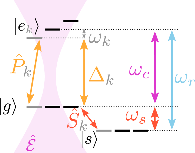
Figure S3: Level structure and notations in the rotating frame.

Conventions, units and experimental values for all relevant parameters are provided in Appendix G. What is more, we should recap the hypotheses that were used:

1. Dipole approximation and Rotating-wave approximation (RWA) for the interaction between the fields and the atoms

2. Homogeneous coupling $g$ for all the atoms

3. Only one well defined cavity light mode couples to only one atomic transition

Let us further assume that

1. Low excitation number (or weak excitation limit) Almost all atoms stay in the ground state at all times, so that, for each atom class $k$, one takes the approximations $\hat{\sigma}_{gg}^{(k)}\approx N_{k}\mathds{I}$ and $\hat{\sigma}_{ee}^{(k)}\approx\mathds{O}$, $\hat{\sigma}_{ss}^{(k)}\approx\mathds{O}$, $\hat{\sigma}_{es}^{(k)}\approx\mathds{O}$ (or more precisely $\frac{1}{N_{k}}\hat{\sigma}_{ee}^{(k)}=\mathcal{O}\left(\frac{1}{N_{k}}\right)$); this is in the end relevant to compute expectation values by discarding higher order terms. Such an approximation typically assumes that each atomic frequency class is sufficiently populated compared to the amount of excitations involved in the system: the approximation does not refer to a single atom operator, but to the frequency class collective operator which is the sum of single-atom operators over the class. It is sufficient to assume that the number of excitations is much smaller than $N$ if no class is much more likely to interact with light than some others. In the situation we are interested in, the number of excitations will be $1$, and a similar approximation can be made exact regardless of the value of $N$ for the purpose of following calculations. A consequence is that the dynamical system for the whole set of operators $\hat{\sigma}_{\alpha,\beta}^{(k)},\quad\alpha,\beta\in\left\{g,e,s\right\}$ given by Hamiltonian evolution is reduced to a set of equations involving $\hat{\mathcal{E}}$ and $\hat{P}_{k},\hat{S}_{k}$ coherences only, where the latter collective operators will behave as bosonic operators, as we will see below.

In order to switch to a rotating frame, we introduce the following slowly-varying operators in the Heisenberg picture:

• $\hat{\mathcal{E}}(t)=e^{+i\omega_{c}t}\hat{a}(t)$ for the cavity field;

• $\hat{P}_{k}(t)=\frac{1}{\sqrt{N_{k}}}e^{+i\omega_{c}t}\hat{\sigma}_{ge}^{(k)}(t)$ for the atomic polarisations;

• $\hat{S}_{k}(t)=\frac{1}{\sqrt{N_{k}}}e^{+i(\omega_{c}-\omega_{r})t}\hat{\sigma}_{gs}^{(k)}(t)$ for the spin polarisations;

• $\hat{C}_{k}(t)=\frac{1}{\sqrt{N_{k}}}e^{+i\omega_{r}t}\hat{\sigma}_{se}^{(k)}(t)\approx\mathds{O}$ with 7.

Those unitary transformations and hypotheses ensure that the following commutation relations hold:

$$\left[\hat{\mathcal{E}}(t),\hat{\mathcal{E}}(t)^{\dagger}\right]=\mathds{I},$$ (22)

and for all $k,j$

$$\left[\hat{P}_{k}(t),\hat{P}_{j}(t)^{\dagger}\right] =\frac{1}{\sqrt{N_{k}N_{j}}}\left[\sum_{l=1}^{N_{k}}|g\rangle_{ll}\langle e|,\sum_{m\text{=}1}^{N_{j}}|e\rangle_{mm}\langle g|\right]$$

$$=\frac{1}{N_{k}}\delta_{kj}\left(\hat{\sigma}_{gg}^{(k)}(t)-\hat{\sigma}_{ee}^{(k)}(t)\right)$$

$$\approx\delta_{kj}\mathds{I},$$ (23)

as well as

$$\left[\hat{S}_{k}(t),\hat{S}_{j}(t)^{\dagger}\right]\approx\delta_{kj}\mathds{I},$$ (24)

where the two later results make use of the low excitation number hypothesis 7. Furthermore, for every $k$, 7 leads to the approximations

$$\left[\hat{P}_{k},\hat{S}_{k}^{\dagger}\right] = \frac{1}{N_{k}}e^{+i\omega_{c}t}e^{-i(\omega_{c}-\omega_{r})t}\sum_{j,l}\left[|g\rangle_{jj}\langle e|,|s\rangle_{ll}\langle g|\right]$$

$$= -\frac{1}{N_{k}}e^{+i\omega_{r}t}\sum_{j}|s\rangle_{jj}\langle e|=-\frac{1}{\sqrt{N_{k}}}\hat{C}_{k}\approx\mathds{O},$$

$$\left[\hat{P}_{k},\hat{P}_{k}^{\dagger}\hat{S}_{k}\right] = \left[\hat{P}_{k},\hat{P}_{k}^{\dagger}\right]\hat{S}_{k}+\hat{P}_{k}^{\dagger}\left[\hat{P}_{k},\hat{S}_{k}\right]\approx\hat{S}_{k}+\mathds{O},$$

$$\left[\hat{S}_{k},\hat{S}_{k}^{\dagger}\hat{P}_{k}\right] = \left[\hat{S}_{k},\hat{S}_{k}^{\dagger}\right]\hat{P}_{k}+\hat{S}_{k}^{\dagger}\left[\hat{S}_{k},\hat{P}_{k}\right]\approx\hat{P}_{k}+\mathds{O},$$

$$\left[\hat{P}_{k},\hat{S}_{k}^{\dagger}\hat{P}_{k}\right] =\left[\hat{P}_{k},\hat{S}_{k}^{\dagger}\right]\hat{P}_{k}+\hat{S}_{k}^{\dagger}\left[\hat{P}_{k},\hat{P}_{k}\right]$$

$$=-\frac{1}{\sqrt{N_{k}}}\hat{C}_{k}\hat{P}_{k}\approx\mathds{O},$$

$$\left[\hat{S}_{k},\hat{P}_{k}^{\dagger}\hat{S}_{k}\right] = \left[\hat{S}_{k},\hat{P}_{k}^{\dagger}\right]\hat{S}_{k}+\hat{P}_{k}^{\dagger}\left[\hat{S}_{k},\hat{S}_{k}\right]$$

$$= -\frac{1}{\sqrt{N_{k}}}\hat{C}_{k}^{\dagger}\hat{S}_{k}+\mathds{O}\approx\mathds{O},$$

and

$$\left[\hat{S}_{k},\hat{P}_{k}^{\dagger}\hat{P}_{k}\right] = \left[\hat{S}_{k},\hat{P}_{k}^{\dagger}\right]\hat{P}_{k}+\hat{P}_{k}^{\dagger}\left[\hat{S}_{k},\hat{P}_{k}\right]\approx\mathds{O}.$$

The definitions for the slowly varying operators amount to switching to a rotating frame. In this new frame, we obtain an effective Hamiltonian

$$\hat{H}_{eff}=\hbar\sum_{k}\omega_{k}\hat{P}_{k}^{\dagger}\hat{P}_{k}-\hbar g\sqrt{N}\sum_{k}\sqrt{n_{k}}\left(\hat{\mathcal{E}}\hat{P}_{k}^{\dagger}+\hat{\mathcal{E}}^{\dagger}\hat{P}_{k}\right)-\frac{\hbar}{2}\sum_{k}\left(\Omega(t)\hat{P}_{k}^{\dagger}\hat{S}_{k}+\Omega^{*}(t)\hat{S}_{k}^{\dagger}\hat{P}_{k}\right),$$ (25)

where we set $\omega_{k}:=\Delta_{k}-\omega_{c}$ for the detuning of class $k$ $|e\rangle-$level w.r.t. the cavity field frequency $\omega_{c}$. Indeed, we show below the dynamics resulting from Heisenberg equation $i\hbar\frac{\mathrm{d}\hat{A}}{\mathrm{d}t}=i\hbar\frac{\partial\hat{A}}{\mathrm{\partial}t}+\left[\hat{A},\hat{H}\right]$ are also given by setting $i\hbar\frac{\mathrm{d}\hat{A}}{\mathrm{d}t}:=\left[\hat{A},\hat{H}_{eff}\right]$ for any operator $\hat{A}=\hat{\mathcal{E}},\hat{P}_{k},\hat{S}_{k}$. On the one hand, we have

$$i\hbar\frac{\mathrm{d}\hat{\mathcal{E}}}{\mathrm{d}t}(t) =i\hbar\left(+i\omega_{c}\right)\hat{\mathcal{E}}(t)+e^{+i\omega_{c}t}\left[\hat{a},\hat{H}\right]$$

$$=-\hbar\omega_{c}\hat{\mathcal{E}}(t)+\hbar\omega_{c}\hat{\mathcal{E}}-e^{+i\omega_{c}t}\hbar g\sum_{k}\hat{\sigma}_{ge}^{(k)}$$

$$=-\hbar g\sqrt{N}\sum_{k}\sqrt{n_{k}}\hat{P}_{k},$$ (26)

and for any index $k$,

$$i\hbar\frac{\mathrm{d}\hat{P}_{k}}{\mathrm{d}t}(t) =i\hbar\left(+i\omega_{c}\right)\hat{P}_{k}(t)+\frac{1}{\sqrt{N_{k}}}e^{+i\omega_{c}t}\left[\hat{\sigma}_{ge}^{(k)},\hat{H}\right]$$

$$=-\hbar\omega_{c}\hat{P}_{k}(t)+\hbar\Delta_{k}\frac{1}{\sqrt{N_{k}}}e^{+i\omega_{c}t}\hat{\sigma}_{ge}^{(k)}-\hbar g\frac{1}{\sqrt{N_{k}}}e^{+i\omega_{c}t}\hat{a}\left(\hat{\sigma}_{gg}^{(k)}-\hat{\sigma}_{ee}^{(k)}\right)-\frac{\hbar}{2}\Omega(t)e^{-i\omega_{r}t}\frac{1}{\sqrt{N_{k}}}e^{+i\omega_{c}t}\hat{\sigma}_{gs}^{(k)}$$

$$\approx\hbar\omega_{k}\hat{P}_{k}(t)-\hbar g\sqrt{N}\sqrt{n_{k}}\hat{\mathcal{E}}(t)-\frac{\hbar}{2}\Omega(t)\hat{S}_{k}(t)\text{ thanks to \ref{enu:Low-excitation-number}},$$ (27)

$$i\hbar\frac{\mathrm{d}\hat{S}_{k}}{\mathrm{d}t}(t) =i\hbar\left(+i(\omega_{c}-\omega_{r})\right)\hat{S}_{k}(t)+\frac{1}{\sqrt{N_{k}}}e^{+i(\omega_{c}-\omega_{r})t}\left[\hat{\sigma}_{gs}^{(k)},\hat{H}\right]$$

$$=-\hbar(\omega_{c}-\omega_{r})\hat{S}_{k}(t)-\hbar\omega_{s}\frac{1}{\sqrt{N_{k}}}e^{+i(\omega_{c}-\omega_{r})t}\hat{\sigma}_{gs}^{(k)}+\hbar g\frac{1}{\sqrt{N_{k}}}e^{+i(\omega_{c}-\omega_{r})t}\hat{a}\hat{\sigma}_{es}^{(k)}-\frac{\hbar}{2}\Omega^{*}(t)e^{+i\omega_{r}t}\frac{1}{\sqrt{N_{k}}}e^{+i(\omega_{c}-\omega_{r})t}\hat{\sigma}_{ge}^{(k)}$$

$$=-\frac{\hbar}{2}\Omega^{*}(t)\hat{P}_{k}(t)\text{ thanks to Eq.~\ref{eq:frequency_sum} and \ref{enu:Low-excitation-number}.}$$ (28)

On the other hand, we have

$$\left[\hat{\mathcal{E}},\hat{H}_{eff}\right]=-\hbar g\sqrt{N}\sum_{k}\sqrt{n_{k}}\hat{P}_{k},$$

and for every $k$

$$\left[\hat{P}_{k},\hat{H}_{eff}\right]\approx\hbar\omega_{k}\hat{P}_{k}-\hbar g\sqrt{N}\sqrt{n_{k}}\hat{\mathcal{E}}-\frac{\hbar}{2}\Omega(t)\hat{S}_{k}\text{ with \ref{enu:Low-excitation-number}}$$ (29)

$$\left[\hat{S}_{k},\hat{H}_{eff}\right]\approx-\frac{\hbar}{2}\Omega^{*}(t)\hat{P}_{k}\text{ with \ref{enu:Low-excitation-number}},$$ (30)

which correspond to Eqs. 26, 27, 28.

Note that the number of total excitations is conserved throughout evolution. Indeed, the total number of excitations operator

$$\hat{N}_{tot}=\hat{\mathcal{E}}^{\dagger}\hat{\mathcal{E}}+\sum_{k}\hat{P}_{k}^{\dagger}\hat{P}_{k}+\sum_{k}\hat{S}_{k}^{\dagger}\hat{S}_{k}$$ (31)

commutes with the effective Hamiltonian, a fortiori thanks to 7,

$$\left[\hat{N}_{tot},\hat{H}_{eff}\right]=\mathds{O}.$$

Adjunction of Langevin noise operators and input-output relations

With the aim of including losses, we turn again to Equations 26, 27 and 28. To that Hamiltonian evolution, one should add non-Hermitian behaviours from the losses and input-output from the cavity, as well as dephasing of atomic polarisations. Related terms will be directly inserted into the equations of motion below.

Following Refs. [39, 40], we introduce different noise operators [55, 38] related to:

• Input-output relations [56, 57, 36, 37], that represent the coupling between the cavity mode and some external degrees of freedom with rate $\kappa$. This will let us describe input and output photons involved in the storage and retrieval processes. Construction of the related $\hat{\mathcal{E}}_{in}(t)$ and $\hat{\mathcal{E}}_{out}(t)$ operators for all times $t$ is discussed in Sec. C.2;

• Possible decay of the $\hat{P}_{k}$ coherences, phenomenologically decribed by the coupling to some external baths $\hat{F}_{P,k}(t)$ with rate $\gamma_{P}$;

• Possible decay of the $\hat{S}_{k}$ coherences, phenomenologically decribed by the coupling to some external baths $\hat{F}_{S,k}(t)$ with rate $\gamma_{P}$.

The decay rates are assumed to be the same for all frequency classes. Other sources of loss are discarded here, such as any further decay channel of the cavity optical mode. Details for the introduction of noise operators and quantum reservoirs are provided in Sec. C.1 of these Appendices, see especially Eqs. 75 and 82. In particular, some specific properties and hypotheses are introduced there, such as the Markovian hypothesis (21) for the reservoirs.

Equations of motions

We end up with the following set of equations of motion, including noise terms,

$$\dot{\mathcal{\hat{\mathcal{E}}}}(t) = -\kappa\hat{\mathcal{E}}(t)+ig\sqrt{N}\sum_{k}\sqrt{n_{k}}\hat{P}_{k}(t)+ +\sqrt{2\kappa}\hat{\mathcal{E}}_{in}(t)$$

$$\dot{\hat{P}}_{k}(t) = -(\gamma_{P}+i\omega_{k}))\hat{P_{k}}(t)+ig\sqrt{N}\sqrt{n_{k}}\hat{\mathcal{E}}(t) +i\frac{\Omega(t)}{2}\hat{S}_{k}(t) +\sqrt{2\gamma_{P}}\hat{F}_{P,k}(t)$$ (32)

$$\dot{\hat{S}}_{k}(t) = -\gamma_{S}\hat{S}_{k}(t) +i\frac{\Omega^{*}(t)}{2}\hat{P}_{k}(t) +\sqrt{2\gamma_{S}}\hat{F}_{S,k}(t)$$

$$\hat{\mathcal{E}}_{out}(t) = \sqrt{2\kappa}\hat{\mathcal{E}}(t)-\hat{\mathcal{E}}_{in}(t)$$ .

If $\gamma_{P}=\gamma_{S}=0$, a conservation law similar to 31 still holds, now including input and output fields:

$$\forall t\quad\frac{\mathrm{d}}{\mathrm{d}t}\left[\hat{\mathcal{E}}^{\dagger}\hat{\mathcal{E}}+\sum_{k}\hat{P}_{k}^{\dagger}\hat{P}_{k}+\sum_{k}\hat{S}_{k}^{\dagger}\hat{S}_{k}+\int_{t}^{+\infty}\hat{\mathcal{E}}_{in}^{\dagger}(t^{\prime})\hat{\mathcal{E}}_{in}(t^{\prime})\mathrm{d}t^{\prime}+\int_{-\infty}^{t}\hat{\mathcal{E}}_{out}^{\dagger}(t^{\prime})\hat{\mathcal{E}}_{out}(t^{\prime})\mathrm{d}t^{\prime}\right](t)=\mathds{O}.$$ (33)

If we are to follow the noise operators, the total number operator is given by

$$\hat{N}_{tot} = \quad\hat{\mathcal{E}}^{\dagger}\hat{\mathcal{E}}+\sum_{k}\hat{P}_{k}^{\dagger}\hat{P}_{k}+\sum_{k}\hat{S}_{k}^{\dagger}\hat{S}_{k}$$

$$+\int_{t}^{+\infty}\hat{\mathcal{E}}_{in}^{\dagger}(t^{\prime})\hat{\mathcal{E}}_{in}(t^{\prime})\mathrm{d}t^{\prime}+\int_{-\infty}^{t}\hat{\mathcal{E}}_{out}^{\dagger}(t^{\prime})\hat{\mathcal{E}}_{out}(t^{\prime})\mathrm{d}t^{\prime}$$

$$+\hat{N}_{bath}$$

with $\hat{N}_{bath}$ the number operator that counts for excitations that left to the reservoirs, which we do not explicit here but such that $\hat{N}_{tot}$ is conserved throughout evolution.

Equivalently, we can use a continuous description of the dynamical system

$$\dot{\hat{\mathcal{E}}}(t) = -\kappa\hat{\mathcal{E}}(t)+igN\int n(\omega)\hat{P}_{\omega}(t)\mathrm{d}\omega +\sqrt{2\kappa}\hat{\mathcal{E}}_{in}(t)$$

$$\dot{\hat{P}}_{\omega}(t) = -(\gamma_{P}+i\omega)\hat{P}_{\omega}(t)+ig\hat{\mathcal{E}}(t) +i\frac{\Omega(t)}{2}\hat{S}_{\omega}(t) +\sqrt{2\gamma_{P}}\hat{F}_{P,\omega}(t)$$ (35)

$$\dot{\hat{S}}_{\omega}(t) = -\gamma_{S}\hat{S}_{\omega}(t) +i\frac{\Omega^{*}(t)}{2}\hat{P}_{\omega}(t) +\sqrt{2\gamma_{S}}\hat{F}_{S,\omega}(t)$$

$$\hat{\mathcal{E}}_{out}(t) = \sqrt{2\kappa}\hat{\mathcal{E}}(t)-\hat{\mathcal{E}}_{in}(t),$$ .

where the correspondance between systems 32 and 35 is described through

$$n(\omega)\mathrm{d}\omega\equiv\sum n_{k}\delta(\omega=\omega_{k})$$

so that

$$\int_{\mathbb{R}}n(\omega)\mathrm{d}\omega=\sum_{k}n_{k}=1,$$ (36)

and by the fact that $\hat{P}_{\omega}$ is associated to the atomic coherences of the $|g\rangle$-$|e\rangle$ transition in the frequency range $[\omega,\omega+\mathrm{d}\omega]$

$$\hat{P}_{k}=\frac{1}{\sqrt{n_{k}N}}e^{+i\omega_{c}t}\sum_{j}^{N_{k}}|g\rangle_{jj}\langle e|\equiv\sqrt{n_{k}N}\hat{P}_{\omega_{k}}\delta(\omega=\omega_{k})$$

and similarly for $\hat{S}_{\omega}$.

B.1.2 Scalar set of equations

Equations 32 and 35 involve quantum operators acting on the whole Hilbert space 14. Further analysis and numerical simulations will instead involve differential equations for scalar functions. In Sec.D, and in particular in part D.4.3, we consider particular conditions requiring that we start from an initially factorised state between the system and the environment (106 and 107), we work within the one-excitation subspace and the memory is loaded with a pure state (109), noise operators follow bosonic commutation rules (110), reservoirs (bar the input-output one) are in the ground state (112), and the memory is initially empty (125). Those particular conditions, together with assumptions made about the noise operators (20, 21, 22 of Appendix C), ensure that we can compute all second-order correlators directly from the integration of some scalar systems of ordinary differential equations, namely

$$\dot{\mathcal{E}}(t) = -\kappa\mathcal{E}(t)+ig\sqrt{N}\sum_{j}\sqrt{p_{j}}P_{j}(t)+\sqrt{2\kappa}\mathcal{E}_{in}(t)$$

$$\dot{P_{k}}(t) = -(\gamma_{P}+i\omega_{k})P_{k}(t)+ig\sqrt{N}\sqrt{n_{k}}\mathcal{E}(t)+\frac{i}{2}\Omega(t)S_{k}(t)$$

$$\dot{S_{k}}(t) = -\gamma_{S}S_{k}(t)+\frac{i}{2}\Omega^{*}(t)P_{k}(t)$$

$$\mathcal{E}_{out}(t) = \sqrt{2\kappa}\mathcal{E}(t)-\mathcal{E}_{in}(t)$$ (37)

or

$$\dot{\mathcal{E}}(t) = -\kappa\mathcal{E}(t)+igN\int n(\omega)P_{\omega}(t)\mathrm{d}\omega+\sqrt{2\kappa}\mathcal{E}_{in}(t)$$

$$\dot{P_{\omega}}(t) = -(\gamma_{P}+i\omega)P_{\omega}(t)+ig\mathcal{E}(t)+\frac{i}{2}\Omega(t)S_{\omega}(t)$$

$$\dot{S_{\omega}}(t) = -\gamma_{S}S_{\omega}(t)+\frac{i}{2}\Omega^{*}(t)P_{\omega}(t)$$

$$\mathcal{E}_{out}(t) = \sqrt{2\kappa}\mathcal{E}(t)-\mathcal{E}_{in}(t).$$ (38)

The former set of equations 37 is easier use for the purpose of numerical resolution with a discretised density (see Sec. H), while the latter 38 is easier to handle analytically as we will do below.

Furthermore, we will argue in Appendix F that those second-order correlators are sufficient to characterise single-photon components that may be emitted by the memory. Within this picture, single-photon wavepackets enter and exit the quantum memory, and $\mathcal{E}_{in}(t)$ represents the input single-photon envelope while $\mathcal{E}_{out}(t)$ represents the output-single photon envelope. For instance, we will start from the pure state

$$|\psi_{input}\rangle=\int\mathcal{E}_{in}(t)\hat{\mathcal{E}}_{in}^{\dagger}(t)|0\rangle\mathrm{d}t$$ (39)

or equivalently

$$|\psi_{input}\rangle=\hat{\mathcal{E}}_{input}^{\dagger}(t)|0\rangle,$$ (40)

where $\hat{\mathcal{E}}_{input}^{\dagger}=\int\mathcal{E}_{in}(t)\hat{\mathcal{E}}_{in}^{\dagger}(t)\mathrm{d}t$ is the creation operator for a photon wavepacket in the mode with temporal shape $\mathcal{E}_{in}$ and $|0\rangle$ is the vacuum state shared by every mode in this linear setting [44].

Though our work focuses on the single-photon regime, we stress that similar sets of equations are obtained if one takes a coherent state as an input for the quantum memory, provided 7 still holds. In that situation $\mathcal{E}_{in/out}(t)$ would represent the envelopes of input/output coherent states (see part D.4.4).

We add initial conditions (say at time $t=t_{0}$) corresponding to an incoming single-photon state towards an empty cavity and an empty memory,

$$\forall k\quad\begin{cases}\mathcal{E}(t_{0})&=0\\ P_{k}(t_{0})&=0\\ S_{k}(t_{0})&=0\end{cases}$$ (41)

with $\mathcal{E}_{in}(t)$ representing the waveform envelope of this incoming single-photon, with $\mathcal{E}_{in}(t<t_{0})=0$. In particular, the conservation equation 33 becomes

$$\forall t\geq 0\quad\left|\mathcal{E}(t)\right|^{2}+\sum_{k}\left|P_{k}(t)\right|^{2}+\sum_{k}\left|S_{k}(t)\right|^{2}+\int_{t_{0}}^{t}\left|\mathcal{E}_{out}(t)\right|^{2}\mathrm{d}t+\int_{t}^{+\infty}\left|\mathcal{E}_{in}(t)\right|^{2}\mathrm{d}t=1,$$ (42)

where we assumed that $\gamma_{P}=\gamma_{S}=0$ and that the input wavepacket is normalised

$$\int_{t_{0}}^{+\infty}\left|\mathcal{E}_{in}(t)\right|^{2}\mathrm{d}t=\int_{-\infty}^{+\infty}\left|\mathcal{E}_{in}(t)\right|^{2}\mathrm{d}t=1.$$ (43)

B.2 Two-level structure and echoes

We now turn to the analytical resolution of system 38 in the context where $n(\omega)$ is chosen to represent an atomic frequency comb (AFC). At first, we only focus on the inhomogeneous $|g\rangle$-$|e\rangle$ two-level structure to introduce the notions of AFC echoes and of impedance-matching regime. Building upon the existing literature, we provide more general formulas to describe such phenomenons. The full $\Lambda$-structure, that enables on-demand readout from the memory, will be discussed in Sec. B.3.

B.2.1 Comb structure of the atomic density

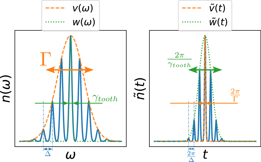
Figure S4: Comb structure $n(\omega)$ and its Fourier transform $\tilde{n}(t)$, with the characteristic widths involved.

We start with the description of the normalised atomic density $n(\omega)$ (see Eq. 36). In order to represent an AFC structure [25, 30, 31] (see Fig. S4), we take $n(\omega)$ as a series of well-separated peaks $w(\omega)$ (typical width $\gamma_{tooth}$) and enveloped by a function $v(\omega)$ (typical width and variation scale $\Gamma$), that is

$$n(\omega) =Z\times v(\omega)\times\sum_{n=-\infty}^{+\infty}w(\omega-n\Delta)$$ (44)

$$=Z\times\left(v\times\left[\mathrm{III}_{\Delta}*w\right]\right)(\omega).$$

A convolution product is noted $*$, $\mathrm{III}(\omega)$ stands for the infinite Dirac comb of step $\Delta$ i.e. $\mathrm{III}(\omega)=\sum_{n=-\infty}^{+\infty}\delta(\omega=n\Delta)$, and $Z$ is a normalisation constant such that Eq. 36 holds. Typically, $v$ can be associated to the inhomogeneously broadened distribution of the atomic ensemble [40, 30, 33], while $w$ gives the shape of the comb teeth that are carved within the inhomogeneous distribution with particular optical pumping techniques such as spectral hole burning [58, 59, 60].

If we assume that $\Gamma\gg\Delta>\gamma_{tooth}$ for a well-defined comb so that the variations of $v$ are slow compared to those of $w$, we can write

$$v(\omega)\times\sum_{n=-\infty}^{+\infty}w(\omega-n\Delta) \approx\sum_{n=-\infty}^{+\infty}v(n\Delta)w(\omega-n\Delta)$$

$$\approx\frac{1}{\Delta}\int_{-\infty}^{+\infty}v(x)w(\omega-x)\mathrm{d}x,$$

so that

$$\int_{-\infty}^{+\infty}n(\omega)\mathrm{d}\omega \approx\frac{Z}{\Delta}\int_{-\infty}^{+\infty}\int_{-\infty}^{+\infty}v(x)w(\omega-x)\mathrm{d}x\mathrm{d}\omega$$

$$=\frac{Z}{\Delta}\int_{-\infty}^{+\infty}w(\omega^{\prime})\mathrm{d}\omega^{\prime}\int_{-\infty}^{+\infty}v(x)\mathrm{d}x.$$

Hence, taking

$$Z=\frac{\Delta}{\int w(\omega)\mathrm{d}\omega\times\int v(\omega)\mathrm{d}\omega}$$ (45)

leads to $\int_{-\infty}^{+\infty}n(\omega)\mathrm{d}\omega\approx 1$. To characterise the comb, we may define the comb finesse [30] as the ratio of the distance between comb teeth over the width of comb teeth,

$$F_{AFC}:=\frac{\Delta}{\mathrm{FWHM}_{teeth}}.$$ (46)

It will also be useful to manipulate the Fourier transform $\tilde{n}(t)$ of $n(\omega)$, which involves the Fourier transforms $\tilde{v}(t)$ and $\tilde{w}(t)$ of $v(\omega)$ and $w(\omega)$. Convolution representation of $n$ leads to

$$\tilde{n}(t) \propto \left(\tilde{v}*\left[\mathrm{III}_{\frac{2\pi}{\Delta}}\times\tilde{w}\right]\right)(t)$$ (47)

$$\propto \int_{-\infty}^{+\infty}\tilde{v}(t-t^{\prime})\times\left(\sum_{n=-\infty}^{+\infty}\delta(t^{\prime}=n\frac{2\pi}{\Delta})\right)\times\tilde{w}(t^{\prime})\mathrm{d}t^{\prime}$$

$$\propto \sum_{n=-\infty}^{+\infty}\int_{-\infty}^{+\infty}\tilde{v}(t-t^{\prime})\delta(t^{\prime}=n\frac{2\pi}{\Delta})\tilde{w}(t^{\prime})\mathrm{d}t^{\prime}$$

$$\propto \sum_{n=-\infty}^{+\infty}\tilde{v}(t-n\frac{2\pi}{\Delta})\tilde{w}(n\frac{2\pi}{\Delta})$$

$$\approx: Y\times\tilde{w}(t)\times\sum_{n=-\infty}^{+\infty}\tilde{v}(t-n\frac{2\pi}{\Delta}),$$

where the last approximation can be made if $\tilde{v}$ is peaked w.r.t. characteristic variations of $\tilde{w}$, that is still ensured by the assumption $\Gamma\gg\Delta>\gamma_{tooth}$. Thus, $\tilde{n}(t)$ also has a comb structure, with step $\frac{2\pi}{\Delta}$ (see Fig. S4). The normalisation constant $Y$ is computed thanks to some Fourier transform identities,

$$Y=Z\times\underset{\times\text{ to }*}{\underbrace{\frac{1}{2\pi}}}\times\underset{\text{Comb}}{\underbrace{\frac{2\pi}{\Delta}}}=\frac{Z}{\Delta}.$$ (48)

The factor $1/2\pi$ comes from the Fourier transform of the convolution product, while the $2\pi/\Delta$ factor stems from the Fourier transform of the Dirac comb.

The area of the central tooth of the comb Fourier transform is defined as

$$D_{comb} :=Y\tilde{w}(0)\int\tilde{v}(t)\mathrm{d}t=\frac{\tilde{w}(t=0)\int\tilde{v}(t)\mathrm{d}t}{\int w(\omega)\mathrm{d}\omega\times\int v(\omega)\mathrm{d}\omega}$$

$$=\frac{\int\tilde{v}(t)\mathrm{d}t}{\int v(\omega)\mathrm{d}\omega}.$$ (49)

We used the fact for any $w$

$$\int_{-\infty}^{+\infty}w(\omega)\mathrm{d}w=\tilde{w}(t=0),$$ (50)

so that $D_{comb}$ value is independent of $w$.

Similarly,

$$\int_{-\infty}^{+\infty}\tilde{w}(t)\mathrm{d}t=2\pi\times w(\omega=0).$$ (51)

In particular, around teeth at $t=k\frac{2\pi}{\Delta}$, we get the peak approximation

$$\tilde{n}(t\approx k\frac{2\pi}{\Delta}) \approx \frac{\tilde{w}(k\frac{2\pi}{\Delta})}{\tilde{w}(0)}\frac{\tilde{w}(0)}{\int w(\omega)\mathrm{d}\omega\times\int v(\omega)\mathrm{d}\omega}\tilde{v}(t)$$ (52)

$$\approx \frac{\tilde{w}(k\frac{2\pi}{\Delta})}{\tilde{w}(0)}D_{comb}\delta_{0}(t)$$

where $\delta_{0}$ is a normalised distribution–like Dirac peak approximation similar to the one used in Wigner-Weisskopf theory [61]. In particular, a $\frac{1}{2}$ coefficient appears when one computes a cropped overlap with a slowly varying function $h$,

$$\int_{0}^{+\infty}\delta_{0}(\omega)\times h(\omega)\mathrm{d}\omega=\frac{1}{2}h(0).$$ (53)

We plot in Fig. S5 some particular shapes for the comb distribution, and provide in Table 2 their properties so as to properly define the characteristic widths $\Gamma$ and $\gamma_{tooth}$.

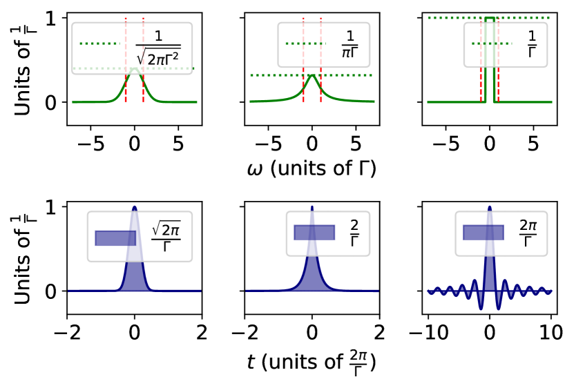
Figure S5: (Top) Comb L1-normalised envelopes, from left to right $u_{Gaussian}(\omega)=\frac{1}{\sqrt{2\pi\Gamma^{2}}}e^{-\frac{\omega{{}^{2}}}{2\Gamma^{2}}}$, $u_{Lorentzian}(\omega)=\frac{1}{\pi\Gamma}\frac{1}{1+\frac{\omega^{2}}{\Gamma^{2}}}$ and $u_{Rect}(\omega)=\frac{1}{\Gamma}\mathds{1}_{\omega\in[-\frac{\Gamma}{2};+\frac{\Gamma}{2}]}$. (Bottom) Fourier transforms of previous functions, respectively $\tilde{u}_{Gaussian}(t)=e^{-\frac{\Gamma^{2}t^{2}}{2}}$, $\tilde{u}_{Lorentzian}(t)=e^{-\Gamma|t|}$ and $\tilde{u}_{Rect}(t)=\mathrm{sinc}\left(\frac{\Gamma t}{2}\right)$. Integrals of the Fourier transforms are provided in the plot legends, while vertical dashed red lines of the top figures indicate $\pm\Gamma$.

Envelope type	Frequency description $u(\omega)$ (characteristic width $\gamma$)	FWHM of $u$	Normalisation $\int{u}(\omega)\mathrm{d}\omega$	Fourier transform $\tilde{u}(t)$	Fourier transform normalisation $\int\tilde{u}(t)\mathrm{d}t$	$D_{comb}=\frac{\int\tilde{u}(t)\mathrm{d}t}{\int u(\omega)\mathrm{d}\omega}$ for $\gamma=\Gamma$	$\mathcal{C}_{opt}:=\frac{2}{\Gamma D_{comb}}$
Dirac peak	$\delta(\omega=0)$	Undefined	$1$	$1$	Undefined, $2\pi$ by convention	Undefined, $2\pi$	Undefined, $\frac{1}{\pi\Gamma}$
Rectangular	$I_{\omega\in[-\frac{\gamma}{2};+\frac{\gamma}{2}]}$	$\gamma$	$\gamma$	$\gamma\mathrm{sinc}\left(\frac{\gamma t}{2}\right)$	$2\pi$	$\frac{2\pi}{\Gamma}$	$\frac{1}{\pi}$
Gaussian	$e^{-\frac{\omega^{2}}{2\gamma^{2}}}$	$2\sqrt{2\ln 2}\gamma$	$\sqrt{2\pi}\gamma$	$\sqrt{2\pi}\gamma e^{-\frac{\gamma^{2}t^{2}}{2}}$	$2\pi$	$\frac{\sqrt{2\pi}}{\Gamma}$	$\sqrt{\frac{2}{\pi}}$
Lorentzian	$\frac{1}{1+\frac{\omega^{2}}{\gamma^{2}}}$	$2\gamma$	$\pi\gamma$	$\pi\gamma e^{-\gamma|t|}$	$2\pi$	$\frac{2}{\Gamma}$	$1$

Table 2: Collection of functions $\omega\mapsto u(\omega)$ that are used to define comb or comb teeth envelopes ($v$ and $w$), see also Fig. S5. Depending on the context, the characteristic width $\gamma\geq 0$ may be understood as $\Gamma$ or $\gamma_{tooth}$. If one does not want to consider distributions centered around $\omega=0$ but rather shifted versions, it is usefull to recall that $\mathrm{TF}(\omega\mapsto f(\omega-a))(t)=e^{-iat}\times\mathrm{TF}(f)(t)$. Last column always features a $2\pi$ thanks to Eq. 51. Another consequence is that $D_{comb}$ value (Eq. 49) only depends on the inhomogeneous envelope $v$, and so does $\mathcal{C}_{opt}$ (Eq. 62).

Finally, note that a comb structure also appears when one introduces a discretised version of an inhomogeneous distribution for numerical resolution, with $w(\omega)=\delta(\omega)$. This situation that involves perfectly narrow teeth corresponds to the set of equations 37.

B.2.2 Absorption and impedance-matching regime

We now look at the consequences the shape $n(\omega)$ has on the dynamics of system 38.

Integration

We start by solving the set of equations to account for absorption of an input pulse by the memory, building upon Refs. [31, 30, 33, 62, 63].

We consider a two-level restriction of Eq. 38, and set $\gamma_{P}=\gamma_{S}=0$, so that

$$\dot{\mathcal{E}}(t) = -\kappa\mathcal{E}(t)+igN\int n(\omega)P_{\omega}(t)\mathrm{d}\omega+\sqrt{2\kappa}\mathcal{E}_{in}(t)$$

$$\dot{P_{\omega}}(t) = -i\omega P_{\omega}(t)+ig\mathcal{E}(t)$$ (54)

$$\mathcal{E}_{out}(t) = \sqrt{2\kappa}\mathcal{E}(t)-\mathcal{E}_{in}(t).$$

Formal integration of $P_{\omega}$ with zero initial conditions 41 at time $t=t_{0}=0$ yields

$$P_{\omega}(t)=ig\int_{t_{0}}^{t}e^{-i\omega(t-t^{\prime})}\mathcal{E}(t^{\prime})\mathrm{d}t^{\prime},$$ (55)

so that for times around $t=t_{0}$ the electric field is given by

$$\dot{\mathcal{E}}(t\approx t_{0}) =-\kappa\mathcal{E}(t)-g^{2}N\int n(\omega)\int_{t_{0}}^{t}e^{-i\omega(t-t^{\prime})}\mathcal{E}(t^{\prime})\mathrm{d}t^{\prime}\mathrm{d}\omega+\sqrt{2\kappa}\mathcal{E}_{in}(t)$$

$$=-\kappa\mathcal{E}(t)-g^{2}N\int_{t_{0}}^{t}\int e^{-i\omega(t-t^{\prime})}n(\omega)\mathrm{d}\omega\mathcal{E}(t^{\prime})\mathrm{d}t^{\prime}+\sqrt{2\kappa}\mathcal{E}_{in}(t)$$ (56)

$$=-\kappa\mathcal{E}(t)-g^{2}N\int_{t_{0}}^{t}\underset{\approx:D_{\mathrm{comb}}\delta_{0}(t-t^{\prime})}{\underbrace{\tilde{n}(t-t^{\prime})}}\mathcal{E}(t^{\prime})\mathrm{d}t^{\prime}+\sqrt{2\kappa}\mathcal{E}_{in}(t)$$ (57)

$$\approx-\kappa\mathcal{E}(t)-g^{2}N\frac{D_{\mathrm{comb}}}{2}\mathcal{E}(t)+\sqrt{2\kappa}\mathcal{E}_{in}(t)\text{ }$$ (58)

where for the last equations we used relations 52 and 53, and the fact that if $t$ is close enough to $t_{0}$ only the central peak of $\tilde{n}(t)$ is involved. If $\mathcal{E}$ varies slowly enough we can set $\dot{\mathcal{E}}(t)\approx 0$ [64, 53, 33]. Then from Eq. 58,

$$\mathcal{E}(t\approx t_{0}) \approx\frac{\sqrt{2\kappa}}{\kappa+g^{2}N\frac{D_{\mathrm{comb}}}{2}}\mathcal{E}_{in}(t)$$

$$=\frac{\sqrt{\frac{2}{\kappa}}}{1+\mathcal{C}\frac{D_{\mathrm{comb}}\Gamma}{2}}\mathcal{E}_{in}(t)$$ (59)

$$=:\frac{\sqrt{\frac{2}{\kappa}}}{1+\frac{\mathcal{C}}{\mathcal{C}_{opt}}}\mathcal{E}_{in}(t)$$ (60)

where we define the memory cooperativity

$$\mathcal{C}:=\frac{g^{2}N}{\kappa\Gamma},$$ (61)

and an optimal cooperativity value

$$\mathcal{C}_{opt}:=\frac{2}{\Gamma D_{comb}}$$ (62)

which only depends on the inhomogeneous envelope shape $v$ (cf. Eq. 49 and Table 2).

Combining Eq. 60 with the input-output relation yields

$$\mathcal{E}_{out}(t) =\mathcal{E}_{in}(t)\times\left(\frac{2}{1+\frac{\mathcal{C}}{\mathcal{C}_{opt}}}-1\right)$$

$$=\mathcal{E}_{in}(t)\times\frac{1-\frac{\mathcal{C}}{\mathcal{C}_{opt}}}{1+\frac{\mathcal{C}}{\mathcal{C}_{opt}}}.$$ (63)

Impedance-matching regime

The situation where

$$\mathcal{C}=\mathcal{C}_{opt}$$ (64)

is called the impedance-matching condition [31, 32, 33], and is characterised by $\mathcal{E}_{out}=0$: no light is reflected back, and equivalently, perfect mapping of the initial input pulse onto atomic collective excitations is achieved. In particular, we can define the absorption efficiency of the memory

$$\eta_{abs} =1-\frac{\int_{t_{0}}^{t_{0}+\Theta}\left|\mathcal{E}_{out}(t)\right|^{2}\mathrm{d}t}{\int_{-\infty}^{+\infty}\left|\mathcal{E}_{in}(t)\right|^{2}\mathrm{d}t}$$

$$=\frac{4\frac{\mathcal{C}}{\mathcal{C}_{opt}}}{\left(1+\frac{\mathcal{C}}{\mathcal{C}_{opt}}\right)^{2}}$$ (65)

where $[t_{0},t_{0}+\Theta]$ encompasses the support of $t\mapsto\mathcal{E}_{in}(t)$, with $\Theta<\frac{2\pi}{\Delta}$. That is, we considered a photon with a long enough frequency bandwidth w.r.t. $\Delta$, with $\mathcal{E}_{in}(t)=0$ when $t<t_{0}$ and $t>t_{0}+\Theta$ (as specified in Eq. 43, $\int_{-\infty}^{+\infty}\left|\mathcal{E}_{in}(t)\right|^{2}\mathrm{d}t=1$). As such, $\eta_{abs}=1$ in the impedance matching condition.

Fourier sampling behaviour

Right after absorption, for $t\gtrsim t_{0}+\Theta$, Eqs. 55 and 60 indicate that the collective polarisation for frequency range $[\omega,\omega+\mathrm{d}\omega]$ is given by

$$P_{\omega}(t\gtrsim t_{0}+\Theta) =\frac{ig\sqrt{\frac{2}{\kappa}}}{1+\frac{\mathcal{C}}{\mathcal{C}_{opt}}}e^{-i\omega t}\int_{-\infty}^{t}e^{+i\omega t^{\prime}}\mathcal{E}_{in}(t^{\prime})\mathrm{d}t^{\prime}$$

$$=\frac{i\sqrt{2\mathcal{C}}\sqrt{\frac{\Gamma}{N}}}{1+\frac{\mathcal{C}}{\mathcal{C}_{opt}}}e^{-i\omega t}\int_{-\infty}^{+\infty}e^{+i\omega t^{\prime}}\mathcal{E}_{in}(t^{\prime})\mathrm{d}t^{\prime}$$

$$=\frac{i2\pi\sqrt{2\mathcal{C}}\sqrt{\frac{\Gamma}{N}}}{1+\frac{\mathcal{C}}{\mathcal{C}_{opt}}}e^{-i\omega t}\mathrm{TF^{-1}}(\mathcal{E}_{in})(\omega)$$

$$=\frac{\sqrt{\frac{\mathcal{C}}{\mathcal{C}_{opt}}}}{1+\frac{\mathcal{C}}{\mathcal{C}_{opt}}}i2\pi\sqrt{2\mathcal{C}_{opt}}\sqrt{\frac{\Gamma}{N}}e^{-i\omega t}\mathrm{TF^{-1}}(\mathcal{E}_{in})(\omega)$$ (66)

i.e.,

$$P_{\omega,opt}(t\gtrsim t_{0}+\Theta)=i\pi\sqrt{2\mathcal{C}_{opt}}\sqrt{\frac{\Gamma}{N}}e^{-i\omega t}\mathrm{TF^{-1}}(\mathcal{E}_{in})(\omega)$$

for the optimal regime where $\mathcal{C}=\mathcal{C}_{opt}$. That is, for a time $t\gtrsim t_{0}+\Theta$ after complete arrival of the wavepacket $\mathcal{E}_{in}$ and before any echo emission (see Sec. B.2.3), we get that each frequency class absorbs energy proportionally to the Fourier coefficient of the envelope profile in the atomic frequency basis. In case of mismatched cooperativity tuning, one gets a detrimental global factor that affects equally all atoms, $\frac{1}{2}\sqrt{\eta_{abs}}$. In particular, for a comb with a rectangular $v$ envelope and $\delta$-peaked teeth $w$, this amounts to computing the Discrete Fourier Transform (DFT) with respect to the atomic frequencies $\omega_{k}=-\frac{\Gamma}{2}+k\frac{\Gamma}{N-1}=-\frac{\Gamma}{2}+k\Delta$, because $\mathcal{C}_{opt}=\frac{1}{\pi}$,

$$P_{\omega_{k},opt,rect}(t) = i\sqrt{2\pi\Delta}\sqrt{\frac{N-1}{N}}\mathrm{TF^{-1}}(\mathcal{E}_{in})(\omega_{k})e^{-i\omega_{k}t}$$ (67)

$$\underset{N\gg 1}{\sim} i\sqrt{2\pi\Delta}\mathrm{TF^{-1}}(\mathcal{E}_{in})(\omega_{k})e^{-i\omega_{k}t}.$$

The result from Eq. 67 is also mentioned in Ref. [63] . It is consistent with the following requirements:

• $\sum_{k}\left|P_{\omega_{k}}\right|^{2}=1$ for perfect absorbtion of a single excitation;

• $\Delta\sum\left|\mathrm{TF^{-1}}(\mathcal{E}_{in})(\omega_{k})\right|^{2}=\frac{1}{2\pi}$ by Parseval–Plancherel identity for the DFT with frequency step $\Delta$.

We can thus provide an interpretation of absorption by the impedance-matched inhomogeneous ensemble as some perfect signal sampling procedure.

In the Schrödinger picture, another way to look at it is to say that the absorption of the incoming photon leads to the creation of a collective excitation delocalised in every atom. The Dicke–like state could write as the collective atomic state

$$\sum_{j=1}^{N}c_{j}e^{-i\omega_{j}t}|g_{1}...g_{j-1}e_{j}g_{j+1}...g_{N}\rangle$$

where $c_{j}$ is proportional to the Fourier coefficient of the photon spectrum in the atomic DFT basis.

After absorption, each frequency class starts dephasing differently from the others ($e^{-i\omega_{k}t}$ term). The resulting collective polarisation is then suppressed so that no light gets out of the memory, until rephasing occurs due to the regular comb structure.

B.2.3 Echoes

We now build upon Refs. [31, 30, 62, 63] to recall that an AFC structure will feature unprompted echoes after absorption of an input pulse [67].

First echo

Let’s focus on the first rephasing (around $t=t_{0}+\frac{2\pi}{\Delta}$). To compute the field, we have to change the initial condition for polarisation. For some time $t_{0}+\Theta\lesssim t_{abs}<t_{0}+\frac{2\pi}{\Delta}$ right after absorption, we know from Eq. 66 that

$$P_{\omega}(t_{abs})=\frac{ig\sqrt{\frac{2}{\kappa}}}{1+\frac{\mathcal{C}}{\mathcal{C}_{opt}}}e^{-i\omega t_{abs}}\int_{-\infty}^{t_{abs}}e^{+i\omega t^{\prime}}\mathcal{E}_{in}(t^{\prime})\mathrm{d}t^{\prime}.$$

Taking this value as an initial condition to integrate Eq. 54 gives at $t\geq t_{abs}$

$$P_{\omega}(t) =ig\int_{t_{abs}}^{t}e^{-i\omega(t-t^{\prime})}\mathcal{E}(t^{\prime})\mathrm{d}t^{\prime}+e^{-i\omega(t-t_{abs})}P_{\omega}(t_{abs})$$

$$=ig\int_{t_{abs}}^{t}e^{-i\omega(t-t^{\prime})}\mathcal{E}(t^{\prime})\mathrm{d}t^{\prime}+ig\frac{\sqrt{\frac{2}{\kappa}}}{1+\frac{\mathcal{C}}{\mathcal{C}_{opt}}}\int_{t_{0}}^{t_{abs}}e^{-i\omega(t-t^{\prime})}\mathcal{E}_{in}(t^{\prime})\mathrm{d}t^{\prime}.$$

Thus, as $\mathcal{E}_{in}(t\geq t_{abs})=0$, Eq. 54 for $t\geq t_{abs}$ is given by

$$\dot{\mathcal{E}}(t) =-\kappa\mathcal{E}(t)+igN\int n(\omega)P_{\omega}(t)\mathrm{d}\omega$$

$$=-\kappa\mathcal{E}(t)-g^{2}N\int_{t_{abs}}^{t}\int n(\omega)e^{-i\omega(t-t^{\prime})}\mathrm{d}\omega\mathcal{E}(t^{\prime})\mathrm{d}t^{\prime}-g^{2}N\frac{\sqrt{\frac{2}{\kappa}}}{1+\frac{\mathcal{C}}{\mathcal{C}_{opt}}}\int_{t_{0}}^{t_{abs}}\int n(\omega)e^{-i\omega(t-t^{\prime})}\mathrm{d}\omega\mathcal{E}_{in}(t^{\prime})\mathrm{d}t^{\prime}$$

$$=-\kappa\mathcal{E}(t)-g^{2}N\int_{t_{abs}}^{t}\tilde{n}(t-t^{\prime})\mathcal{E}(t^{\prime})\mathrm{d}t^{\prime}-g^{2}N\frac{\sqrt{\frac{2}{\kappa}}}{1+\frac{\mathcal{C}}{\mathcal{C}_{opt}}}\int_{t_{0}}^{t_{abs}}\tilde{n}(t-t^{\prime})\mathcal{E}_{in}(t^{\prime})\mathrm{d}t^{\prime}.$$

As explained in Ref. [30], the first integral corresponds to reabsorption of the field while the second one describes the source term, which will lead to the retrieved echo. We now expand $\tilde{n}$ around the relevant peaks: around $t-t^{\prime}=0$ in the first integral, and around $t-t^{\prime}=\frac{2\pi}{\Delta}$ in the second (see Eq. 52). We obtain

$$\dot{\mathcal{E}}(t)\approx-\kappa\mathcal{E}(t)-g^{2}N\frac{D_{\mathrm{comb}}}{2}\mathcal{E}(t)-g^{2}N\frac{\sqrt{\frac{2}{\kappa}}}{1+\frac{\mathcal{C}}{\mathcal{C}_{opt}}}\frac{\tilde{w}(\frac{2\pi}{\Delta})}{\tilde{w}(0)}\times D_{\mathrm{comb}}\mathcal{E}_{in}(t-\frac{2\pi}{\Delta})$$

Neglecting again $\dot{\mathcal{E}}$ and using the input-output relation with zero input (after some time the input pulse is over, i.e. $\mathcal{E}_{in}(t)=0$) leads to the first echo

$$\mathcal{E}_{out}(t\approx t_{0}+\frac{2\pi}{\Delta}) =\sqrt{2\kappa}\mathcal{E}(t\approx t_{0}+\frac{2\pi}{\Delta})$$

$$\approx-\sqrt{2\kappa}\times\frac{1}{\kappa+g^{2}N\frac{D_{\mathrm{comb}}}{2}}\times g^{2}N\frac{\sqrt{\frac{2}{\kappa}}}{1+\frac{\mathcal{C}}{\mathcal{C}_{opt}}}\frac{\tilde{w}(\frac{2\pi}{\Delta})}{\tilde{w}(0)}\times D_{\mathrm{comb}}\times\mathcal{E}_{in}(t-\frac{2\pi}{\Delta})$$

$$=-\frac{\tilde{w}(\frac{2\pi}{\Delta})}{\tilde{w}(0)}\times 2\times\frac{g^{2}ND_{\mathrm{comb}}}{\kappa+g^{2}N\frac{D_{\mathrm{comb}}}{2}}\times\frac{1}{1+\frac{\mathcal{C}}{\mathcal{C}_{opt}}}\times\mathcal{E}_{in}(t-\frac{2\pi}{\Delta})$$

$$=-\frac{\tilde{w}(\frac{2\pi}{\Delta})}{\tilde{w}(0)}\times\frac{4\frac{\mathcal{C}}{\mathcal{C}_{opt}}}{\left(1+\frac{\mathcal{C}}{\mathcal{C}_{opt}}\right)^{2}}\times\mathcal{E}_{in}(t-\frac{2\pi}{\Delta}).$$ (68)

This last equation is consistent with Eq. (10) of Ref. [31]. Note that a $\pi$-phase is included in the reemission of this first echo. What’s more, the first term of Eq. 68 involves the shape of the comb teeth and corresponds to the losses due to non-recurrent atomic dephasing, so we introduce

$$\eta_{F}:=\left(\frac{\tilde{w}(\frac{2\pi}{\Delta})}{\tilde{w}(0)}\right)^{2}.$$ (69)

Of course, for infinitely narrow teeth ($\tilde{w}:t\mapsto 1$) $\eta_{F,\text{perfect}}=1$. On the contrary, for Gaussian teeth ($\tilde{w}:t\mapsto\sqrt{2\pi}\gamma_{tooth}e^{-\frac{\gamma_{tooth}^{2}t^{2}}{2}}$) $\eta_{F,\text{Gaussian}}=e^{-\gamma_{tooth}^{2}\frac{4\pi^{2}}{\Delta^{2}}}=e^{-\frac{4\pi^{2}}{8\ln(2)}\frac{1}{F_{AFC,\mathrm{Gaussian}}^{2}}}\approx e^{-\frac{7}{F_{AFC,\mathrm{Gaussian}}^{2}}}$ which is Eq. (A21) of Ref. [30] and $F_{AFC}$ is the comb finesse (Eq. 46). For rectangular teeth ($\tilde{w}:t\mapsto\gamma\mathrm{sinc}(\frac{\gamma_{tooth}t}{2})$) $\eta_{F,\text{Rect}}=\mathrm{sinc}^{2}\left(\frac{\gamma_{tooth}t}{2}\frac{2\pi}{\Delta}\right)=\mathrm{sinc}^{2}\left(\frac{\pi}{F_{c,\text{Rect}}}\right)$ which corresponds to the last term of Eq. (2) in Ref. [68]. Note that the teeth shape can be optimised to maximise the efficiencies given a particular absorption, see Refs. [69, 70].

The second term of Eq. 68 involves the impedance matching condition and we recognise $\eta_{abs}(\mathcal{C})$ (Eq. 65) so we obtain the efficiency

$$\eta_{\text{1st-echo}} = \frac{\int_{t_{0}+2\pi/\Delta}^{t_{0}+2\pi/\Delta+\Theta}\left|\mathcal{E}_{out}(t)\right|^{2}\mathrm{d}t}{\int_{-\infty}^{+\infty}\left|\mathcal{E}_{in}(t)\right|^{2}\mathrm{d}t}$$

$$= \eta_{F}\times\eta_{abs}{{}^{2}}=\left(\frac{\tilde{w}(\frac{2\pi}{\Delta})}{\tilde{w}(0)}\right)^{2}\times\frac{16\left(\frac{\mathcal{C}}{\mathcal{C}_{opt}}\right)^{2}}{\left(1+\frac{\mathcal{C}}{\mathcal{C}_{opt}}\right)^{4}}.$$

In the case of perfect teeth and impedance matching, we then get unit efficiency in the first echo: the input signal is perfectly reemitted, up to a $\pi$-phase. This observation leads Refs. [69, 71] to interpret the AFC echo as a purely dispersive effect: when the peaks of the AFC are taken infinitely narrow, the power spectrum is almost unchanged (since $n(\omega)$ is zero almost everywhere), and the delay for reemission appears a slow-light effect due to phases acquired along the way.

Further echoes

In case the input signal is not perfectly reemitted in the first echo, some energy remains stored within the collective polarisations. This energy is likely to be reemitted later on, when further echoes happen, as it can be shown by recursively solving the equations around times $k\frac{2\pi}{\Delta}$.

B.2.4 Polarisation decay

So far, we did not take into account the decay channel linked to $\gamma_{P}$. In the case where $\gamma_{P}\neq 0$ is small enough compared to the other dynamical parameters, the influence of polarisation decay can readily be included by introducting an exponential decrease of the rephasing efficiency so that

$$\eta_{tot}(\mathcal{C})\approx\eta_{1st-echo}(\mathcal{C})\times e^{-2\gamma_{P}\frac{2\pi}{\Delta}},$$ (71)

where $\frac{2\pi}{\Delta}$ is the time that the excitation spends in the $P$ coherences.

B.2.5 Bandwidth

The absorption bandwidth of the cavity-enhanced memory can be estimated from the shape of the inhomogeneous distribution $v(\omega)$ and the parameters $\kappa$, $\Gamma$, and $g\sqrt{N}$. As long as the first AFC echo is not involved (short enough input), the AFC comb structure does not matter. In this regard, Ref. [33] provides exact results in the Lorentzian case with $\gamma_{P}=0$, for which the bandwidth is found to be $4\kappa$ when $\kappa<g\sqrt{N}<\Gamma$, and $4\Gamma$ when $\kappa>g\sqrt{N}>\Gamma$ (weak coupling regime). Actually, one can check that the same orders of magnitude hold for Gaussian and rectangular envelopes (up to a similar but different factor than $4$). As noted in Ref. [33], taking the input photon within the memory bandwidth readily ensures that the assumptions $\tilde{n}(t-t^{\prime})\approx D_{comb}\delta_{0}(t-t^{\prime})$ and $\dot{\mathcal{E}}\approx 0$ made in Sec. B.2.2 are met. For our study, relevant experimental parameters (see Appendix G) correspond to the second situation, so we will seek to take small compared to $\Gamma$. This is compatible with $\Delta<\delta\omega_{in}$ provided that the AFC comb has a large enough number of teeth.

B.2.6 Efficient memory

To sum up, optimised absorption of the input pulse requires:

• The impedance-matching condition 64;

• $\frac{2\pi}{\delta\omega_{in}}<\frac{2\pi}{\Delta}$: the pulse is shorter than the echo time. In the sampling picture, this means that the sampling rate should be high enough to represent the shape of the pulse (sort of Shannon-Nyquist theorem);

• That the photon bandwidth shall be smaller than memory bandwidth ($\kappa$ or $\Gamma$ see above), to avoid distortions.

With the impedance-matching condition, the echo is emitted with high efficiency if the teeth of the comb are narrow enough. If the bandwidth of the input is too large, distortions appear.

B.3 Third level and on-demand storage

Now, the full $\Lambda$-system structure of the atoms, including the atomic coherences $S_{\omega}$, is considered (see Fig. S3). Recall that in Eqs. 37 and 38, $\Omega(t)$ represents the time-dependent Rabi frequency for the transfer between $P$ and $S$ coherences. As $P$ coherences are the only ones that couple to the cavity mode and then to the output field, transferring to $S$ coherences enables long storage times.

First, we observe that if $\Omega(t)=0$, the equation for $S_{\omega}$ in system 38

$$\dot{S}_{\omega}(t)=-\gamma_{S}S_{\omega}(t)$$

is integrated as

$$S_{\omega}(t)=e^{-\gamma_{S}t}S_{\omega}(0).$$ (72)

Consequently, this evolution does not depend on $\omega$: no inhomogeneous phase is accumulated. If $\gamma_{S}=0$, no loss occurs and time appears frozen: that is, the coherence will live as long as no transfer is done. Still, we point out that this result is a consequence of the assumption that $|s\rangle$ levels do not exhibit any inhomogeneous broadening w.r.t. the $|g\rangle$ level. In practice, this does not happen and dynamical decoupling methods can be introduced to compensate for dephasing due to inhomogeneous broadening [72, 73].

We can take advantage of the time-freezing property of the $S$ levels to introduce on-demand storage and readout for the quantum memory. To this aim, transfers between $S$ and $P$ are studied.

B.3.1 Transfer to and from spin-levels

Ideal case of closed oscillations

First, we forget about the coupling between $P$ coherences and the field $\mathcal{E}$, and again set $\gamma_{P}=\gamma_{S}=0$. As a consequence, textbook results about Rabi oscillations in the semi-classical regime apply [74, 52]. Considering the situation where the driving $\Omega(t)$ has a rectangular profile, starts at $t_{i}$, is constant of value $\Omega$ for a period of time $T_{R}$ and gets back to $0$ afterwards, we obtain for any time $0\leq t\leq T_{R}$

$$\dot{P_{\omega}}(t_{i}+t) =-i\omega P_{\omega}(t_{i}+t)+\frac{i}{2}\Omega S_{\omega}(t_{i}+t)$$

$$\dot{S_{\omega}}(t_{i}+t) =\frac{i}{2}\Omega^{*}P_{\omega}(t_{i}+t).$$ (73)

Integration of Eqs. 73 from $t_{i}$ to $t_{i}+t$ leads to

$$S_{\omega}(t_{i}+t) =e^{-i\omega t/2}\left(\cos(\Upsilon_{\omega}t/2)+i\frac{\omega}{\Upsilon_{\omega}}\sin(\Upsilon_{\omega}t/2)\right)S_{k}(t_{i})+ie^{-i\omega t/2}\frac{\Omega}{\Upsilon_{\omega}}\sin(\Upsilon_{\omega}t/2)P_{\omega}(t_{i})$$

$$P_{\omega}(t_{i}+t) =ie^{-i\omega t/2}\frac{\Omega}{\Upsilon_{\omega}}\sin(\Upsilon_{\omega}t/2)S_{\omega}(t_{i})+e^{-i\omega t/2}\left(\cos(\Upsilon_{\omega}t/2)-i\frac{\omega}{\Upsilon_{\omega}}\sin(\Upsilon_{\omega}t/2)\right)P_{\omega}(t_{i})$$

where $\Upsilon_{\omega}=\sqrt{\Omega^{2}+\omega^{2}}$ is the generalised Rabi frequency for frequency class of detuning $\omega$. In particular, if $S_{\omega}(t_{i})=0$ then

$$S_{\omega}(t_{i}+T_{R})=ie^{-i\omega T_{R}/2}\frac{\Omega}{\Upsilon_{\omega}}\sin(\Upsilon_{\omega}T_{R}/2)P_{\omega}(t_{i}),$$

which means that the excitation transfer from $P_{\omega}$ to $S_{\omega}$ is

$$\left|\frac{S_{\omega}(t_{i}+T_{R})}{P_{\omega}(t_{i})}\right|^{2} =\frac{\Omega^{2}T_{R}^{2}}{4}\mathrm{sinc}^{2}\left(\Upsilon_{\omega}T_{R}/2\right)$$

$$=\frac{\Omega^{2}T_{R}^{2}}{4}\mathrm{sinc}^{2}\left(\sqrt{\frac{\Omega^{2}T_{R}^{2}}{4}+\frac{\omega^{2}T_{R}^{2}}{4}}\right).$$

An identical result holds for the transfer from $S_{\omega}$ to $P_{\omega}$ if $P_{\omega}(t_{i})=0$ initially.

Now, assume that $T_{R}\ll\frac{2\pi}{\Gamma}$ with $\Gamma$ the ensemble inhomogeneous linewidth ($\omega$ is at most of the order of $\Gamma$). Then whatever the value of $\omega$, the detuning component $\frac{\omega^{2}T_{R}^{2}}{4}\ll 1$ does not affect much the value of population transfer. Hence,

$$\forall\omega\quad\left|\frac{S_{\omega}(t_{i}+T_{R})}{P_{\omega}(t_{i})}\right|^{2} \approx_{T_{R}\ll\frac{2\pi}{\Gamma}}\left|\frac{S_{\omega=0}(t_{i}+T_{R})}{P_{\omega=0}(t_{i})}\right|^{2}$$

$$=\frac{\Omega^{2}T_{R}^{2}}{4}\mathrm{sinc}^{2}\left(\frac{\Omega T_{R}}{2}\right)$$

$$=\sin^{2}\left(\frac{\Omega T_{R}}{2}\right).$$

In particular, for a rectangular $\pi$-pulse ($\Omega T_{R}=\pi$) the excitation transfer is almost perfect for all frequency classes. One can also introduce partial transfers, that we call $a\pi$-pulses for simplicity (with $0\leq a\leq 1$). By setting

$$\Omega T_{R}=:a\pi=2\mathrm{Arcsin}(q),$$ (74)

the excitation transfer is $q^{2}$.

In practice in our context, it is sufficient that $T_{R}$ is chosen much smaller than $\frac{2\pi}{\delta\omega_{in}}$ where $\delta\omega_{in}$ is the bandwidth of the input photon that was stored inside the memory. Indeed, only the frequency classes with $\omega$ at most of the order of $\delta\omega_{in}$ are susceptible to bear relevant amounts of excitation (see par. B.2.2), and performing transfers on those classes only is enough to generate and retrieve a spin wave that represents the entire photon. Numerically, we check that a factor $10$ between the two timescales is enough.

In terms of complex coefficients, we can approximate the transfer function between $P_{\omega}$ and $S_{\omega}$ by

$$H_{P\leftrightarrow S}(\omega)\approx ie^{-i\omega T_{R}/2}\sin(\Omega T_{R}/2)$$

where a frequency-class dependent phase arises. Once again, if $T_{R}\ll\frac{2\pi}{\delta\omega_{in}}$, this inhomogeneous phase shall not affect much the rephasing of the $P_{\omega}$ coherences and coupling to the external field.

This possibility of bringing excitations back and forth between $S$ and $P$ provides a scheme for longer storage. Once the input photon is absorbed onto $P$, a storage $\pi$-pulse is applied before the $\frac{2\pi}{\Delta}$ delay for echo emission (see Fig. 3 in the main text). In our rotating frame, the spin wave then does not accumulate any phase with time. After a certain time, a readout $\pi$-pulse is applied to retrieve the excitation: $P$ coherences phase accumulation resumes and an echo is finally emitted, as if time between the $\pi$-pulses had been frozen. The possibility to choose this duration enables on-demand storage and readout from the memory.

Open system

The dynamics of the real system are more intricate.

To begin with, coherence losses through $\gamma_{P}$ and $\gamma_{S}$ may happen. It turns out that if the loss rates are slow enough ($\gamma_{P,S}<\Omega$, which is the case for our strong pulses) then one stays in a regime known as underdamped [74]. Then the previous analysis still qualitatively holds. Some loss factors would of course be included by hand, similarly to Eq. 71, 72.

Furthermore, $P$ coherences keep interacting with $\mathcal{E}$ field during transfers. We argue that if the transfer pulses are fast enough compared with the coupling time scales $\kappa$ and $g\sqrt{N}$ the former picture still stands, as it is observed on numerical simulations. Moreover, if the transfer pulses are applied much before the echo, we know that inhomogeneous phase spreading on $P_{\omega}$ coherences (see Eq. 67) hamper any coupling with light that could come out of the cavity. As such, the former picture is quite relevant.

To this respect, we note that a naive photon stretching procedure could involve applying longer $\pi$-pulses ($T_{R}$ comparable or longer than $\frac{2\pi}{\delta\omega_{in}}$) so that only the central part of the frequency spectrum would then rephase and be emitted. A drawback of this method is that all the energy carried by discarded frequency classes is lost, the efficiency is low and comparable to the one of filtration of the input photon in the frequency domain. Our more efficient shaping procedure will be presented in Section E of these Appendices.

B.3.2 Multimode compatibility

Freezing time or storing right before an echo (see Fig. 3 of the Main Text) is useful for the use of the AFC memory in a quantum network context, where temporal multiplexing and synchronisation of emitted photons are crucial [13, 75]. The AFC can accept any time bin of arrival within a $\frac{2\pi}{\Delta}$ window. For synchronisation, a first storage $\pi$-pulse is applied before the first possible AFC echo at time $2\pi/\Delta$, possibly without knowing in what precise time bin the input arrived. Once the time bin is known (e. g. by detection of a correlated photon [13]), synchronisation $\pi$-pulses are applied so that the AFC will immediately follow the application of any further retrieval pulse, see Fig. 3 of the main text.

Appendix C Quantum reservoirs

C.1 Quantum noise and fluctuations

In Sec. B and Ref. [39], the Heisenberg-Langevin approach is used to include losses in the dynamical system: decay channels of an open system are represented by the coupling to a large assembly of bosonic oscillators. This assembly is referred to as a quantum reservoir (or bath). From the system perspective, the reservoir induces backaction and gives rise to noise terms in the equations [38], which in turn ensure that commutators between systems operators are preserved despite the decay channels. In this Appendix, we clarify some statements about quantum noise operators for the construction of Heisenberg-Langevin equations 32. To this aim, helpful derivations may be found in Refs. [61], [76], [77], and [78].

A noise term is usually included in the form of a driving term $\hat{F}_{l}(t)$ in the equation of motion of some system operator $\hat{X}_{l}$. That gives

$$\frac{\mathrm{d}\hat{X}_{l}}{\mathrm{d}t}(t)=-\frac{i}{\hbar}\left[\hat{X}_{l},\hat{H}\right](t)-\gamma\hat{X}_{l}(t)+\sqrt{2\gamma}\hat{F}_{l}(t),$$ (75)

where $\hat{H}$ is the Hamiltonian that governs the deterministic evolution of the closed system, and $\gamma$ is the rate of the decay channel associated to noise term $\hat{F}_{l}$.

Moreover, we will make use of the following hypotheses:

1. Reservoir in the ground state hypothesis Noise terms at time $t$, noted $\hat{F}_{l}(t)$, are commonly defined from reservoir operators considered at the initial time $t_{0}$ (see input-output derivations below). Hence, we can characterise the reservoir backaction thanks to the initial conditions and state of the reservoir. Typically, we will assume that the reservoir is initially in the vacuum state and bears no excitation before being coupled with the system .

2. Markovian noise hypothesis If one assumes that the eigenfrequencies of the reservoir oscillators are closely spaced and thus continuously span a broad enough spectrum, and that the coupling constant does not vary much with frequency, some formal integrations à la Wigner-Weisskopf result in a memoryless property of the reservoir. Typically, all second-order correlators involving noise terms are delta-peaked in time: no correlation is found between noise at different times. This property also results in the well-known generalised Einstein relations related to some quantum fluctuation-dissipation result.

3. Uncorrelated reservoir A side assumption is typically that the reservoir and the system are initially uncorrelated: their quantum states are independent. This also explains why for 20 we can define the state of the reservoirs independently.

As recalled in Ref. [39], a consequence of 20, 21 and 22 is that second-order correlators involving noise terms are all zero but the antinormal ordered one:

$$\forall t,t^{\prime}\quad\langle\hat{F_{l}}(t^{\prime})\hat{F_{l}}(t)\rangle=\langle\hat{F_{l}}^{\dagger}(t^{\prime})\hat{F_{l}}(t)\rangle=0,$$

$$\forall t,t^{\prime}\quad\langle\hat{F_{l}}(t^{\prime})\hat{F_{l}}^{\dagger}(t)\rangle\propto\delta(t-t^{\prime}).$$

The coefficient of proportionality of the last equation (also known as the diffusion coefficient) can be found using generalised Einstein relations [55, 77, 61]. In our case, $\hat{X}_{l}$ operators will refer to the $\hat{P}_{k}$ and $\hat{S}_{k}$ collective operators of Appendix B. It turns out that with the right normalisations, assuming that each individual atom is coupled to an independent reservoir, using the low-excitation hypothesis 7, and referring to the generalised Einstein relations for individual operators, the coefficient is $1$ (see Ref. [39] (Eq. (A15) and (A16)), Appendix of Ref. [79]).

Another consequence, related to 20 and 22, is that initial time second-order correlators involving one reservoir operator and one system operator are zero. Specifically, for every $t$

$$\left\langle\hat{X}_{l}(t_{0})\hat{F}_{l}(t)\right\rangle=0$$

Finally, we will assume that any pair of different decay channels is associated to two independent reservoirs, so crossed second-order correlators are also zero (noise terms for $l\neq l^{\prime}$).

C.2 Quantum input-output relations

A particular type of noise is involved in input-output relations [37, 38] (see also Refs. [56, 57, 36, 66, 52]). A typical setting consists of a cavity, open on one side to coupling to an infinite set of free space modes. For instance, consider our cavity mode $\hat{\mathcal{E}}$ and the complete set of free space electromagnetic modes (one-dimensional here) $\hat{c}(\omega)$ for $\omega\in\mathbb{R}$ such that $\forall\omega,\omega^{\prime}\quad\left[\hat{c}(\omega),\hat{c}^{\dagger}(\omega^{\prime})\right]=\delta(\omega-\omega^{\prime})$. We assume that the coupling is introduced through the approximate interaction Hamiltonian

$$\hat{H}_{bath}=\hbar\int\sqrt{\frac{\kappa(\omega)}{\pi}}\left(\hat{\mathcal{E}}\hat{c}^{\dagger}(\omega)+\hat{\mathcal{E}}^{\dagger}\hat{c}(\omega)\right)\mathrm{d}\omega.$$

In case the coupling is set aside, the free space modes are assumed to evolve according to the Hamiltonian $\hbar\int\omega\hat{c}^{\dagger}(\omega)\hat{c}(\omega)\mathrm{d}\omega$ so that their evolution is given by

$$\frac{\mathrm{d}\hat{c}(\omega)}{\mathrm{d}t}(t)=-i\omega\hat{c}(\omega,t)-i\sqrt{\frac{\kappa(\omega)}{\pi}}\hat{\mathcal{E}}(t)$$

that we integrate as

$$\hat{c}(\omega,t)=e^{-i\omega(t-t_{0})}\hat{c}(\omega,t_{0})-i\sqrt{\frac{\kappa(\omega)}{\pi}}\int_{t_{0}}^{t}e^{-i\omega(t-t^{\prime})}\hat{\mathcal{E}}(t^{\prime})\mathrm{d}t^{\prime},$$ (76)

or

$$\hat{c}(\omega,t)=e^{-i\omega(t-t_{f})}\hat{c}(\omega,t_{f})+i\sqrt{\frac{\kappa(\omega)}{\pi}}\int_{t}^{t_{f}}e^{-i\omega(t-t^{\prime})}\hat{\mathcal{E}}(t^{\prime})\mathrm{d}t^{\prime}.$$ (77)

One can define input modes from the free space modes taken at time $t_{0}$ (understood as preceding any interaction) as

$$\hat{\mathcal{E}}_{in}(t)=\frac{-i}{\sqrt{2\pi}}\int e^{-i\omega(t-t_{0})}\hat{c}(\omega,t_{0})\mathrm{d}\omega$$ (78)

so that for all $t,t^{\prime}$

$$\left[\hat{\mathcal{E}}_{in}(t),\hat{\mathcal{E}}_{in}^{\dagger}(t^{\prime})\right] = \frac{1}{2\pi}\int e^{-i\omega(t-t^{\prime})}\mathrm{d}\omega$$

$$= \delta(t-t^{\prime}).$$

Note that this Fourier-transform like operation can be seen as some change of basis. Just as the whole set of free space modes at time $t_{0}$ could be completely described by the collection of $\hat{c}(\omega,t_{0})$ for all $\omega$, it can be completely described by the collection of $\hat{\mathcal{E}}_{in}(t)$ for all $t$.

Similarly, one can define output modes from the free space modes taken at time $t_{f}>t_{0}$ (understood as following any interaction) as

$$\hat{\mathcal{E}}_{out}(t)=\frac{i}{\sqrt{2\pi}}\int e^{-i\omega(t-t_{f})}\hat{c}(\omega,t_{f})\mathrm{d}\omega$$

so that again, for all $t,t^{\prime}$

$$\left[\hat{\mathcal{E}}_{out}(t),\hat{\mathcal{E}}_{out}^{\dagger}(t^{\prime})\right]=\delta(t-t^{\prime}).$$

Thus, the whole set of free space modes at time $t_{f}$ is completely described either by the collection of $\hat{c}(\omega,t_{f})$ for all $\omega$, or by the collection of $\hat{\mathcal{E}}_{out}(t)$ for all $t$.

Then the Markovian approximation assumes that the coupling constant between the cavity mode $\hat{\mathcal{E}}$ and any external mode $\hat{c}(\omega)$ does not depend on the frequency $\omega$ ($\forall\omega\quad\kappa(\omega)=\kappa$) so that $\hat{\mathcal{E}}$ evolves as

$$\frac{\mathrm{d}\hat{\mathcal{E}}}{\mathrm{d}t}(t) = -\frac{i}{\hbar}\left[\hat{\mathcal{E}},\hat{H}+\hat{H}_{bath}\right]$$ (80)

$$= -\frac{i}{\hbar}\left[\hat{\mathcal{E}},\hat{H}\right]-i\sqrt{\frac{\kappa}{\pi}}\int\hat{c}(\omega,t)\mathrm{d}\omega$$

$$= -\frac{i}{\hbar}\left[\hat{\mathcal{E}},\hat{H}\right]-\frac{\kappa}{\pi}\int\int_{t_{0}}^{t}e^{-i\omega(t-t^{\prime})}\hat{\mathcal{E}}(t^{\prime})\mathrm{d}t^{\prime}\mathrm{d}\omega$$

$$-i\sqrt{2\kappa}\frac{1}{\sqrt{2\pi}}\int e^{-i\omega(t-t_{0})}\hat{c}(\omega,t_{0})\mathrm{d}\omega$$

$$= -\frac{i}{\hbar}\left[\hat{\mathcal{E}},\hat{H}\right]-\kappa\hat{\mathcal{E}}(t)+\sqrt{2\kappa}\hat{\mathcal{E}}_{in}(t),$$

where we used Eq. 76 to go from the second to the third line. In Eq. 80, $\hat{H}$ is the Hamiltonian that governs all evolutions but the coupling to the external bath. As such, we retrieve a decay at rate $\kappa$ in terms of field intensity, and the feeding of $\hat{\mathcal{E}}(t)$ with input $\hat{\mathcal{E}}_{in}(t)$. Similarly, one can obtain from Eq. 77

$$\frac{\mathrm{d}\hat{\mathcal{E}}}{\mathrm{d}t}(t)=-\frac{i}{\hbar}\left[\hat{\mathcal{E}},\hat{H}\right]+\kappa\hat{\mathcal{E}}(t)-\sqrt{2\kappa}\hat{\mathcal{E}}_{out}(t).$$ (81)

Equating the right-hand sides of Eqs. 80 and 81 leads to the input-output relation

$$2\kappa\hat{\mathcal{E}}(t)=\sqrt{2\kappa}\left(\hat{\mathcal{E}}_{in}(t)+\hat{\mathcal{E}}_{out}(t)\right)$$

i.e.

$$\hat{\mathcal{E}}_{out}(t)=\sqrt{2\kappa}\hat{\mathcal{E}}(t)-\hat{\mathcal{E}}_{in}(t).$$ (82)

A last thing to note is that input term at $t$ only influences $\hat{\mathcal{E}}$ at times $t^{\prime}\geq t$, as expected for causality [37, 38]. Namely,

$$\left[\hat{\mathcal{E}}_{in}(t),\hat{\mathcal{E}}(t^{\prime})\right]=0,\text{ if {\hbox{t'<t}}}$$

and

$$\left[\hat{\mathcal{E}}_{out}(t),\hat{\mathcal{E}}(t^{\prime})\right]=0,\text{ if {\hbox{t'>t}}}.$$

Finally, $\left[\hat{\mathcal{E}}_{in}(t),\hat{\mathcal{E}}^{(\dagger)}(t_{0})\right]$ and $\left[\hat{\mathcal{E}}_{out}(t),\hat{\mathcal{E}}^{(\dagger)}(t_{f})\right]$ depend on the initial conditons for the system and the set of external free modes: see 22 above.

Appendix D Integration of a set of differential equations for quantum operators

In this Appendix, we explain how the scalar equations 37, 38 are obtained from the equations involving quantum operators 32, 35.

D.1 Integration of a vectorial ODE

To this end, we first recall some textbook results about the integration of vectorial Ordinary Differential Equations (ODEs). In particular, we stress that a formal integration of the ODE shows that any solution is a linear function of the initial conditions.

Let $\mathscr{E}$ be a vector space of finite dimension $n$, typically $\mathscr{E}=\mathbb{C}^{n}$. Consider the first order ODE on $\mathscr{E}$

$$\dot{Y}(t)=M(t)X(t)+F(t),$$ (83)

with $\begin{array}[]{cccc}X:&\mathbb{R}&\rightarrow&\mathscr{E}\\ &t&\mapsto&X(t)\end{array}$,$\begin{array}[]{cccc}M:&\mathbb{R}&\rightarrow&\mathcal{L}(\mathscr{E},\mathscr{E})\\ &t&\mapsto&M(t)\end{array}$and $\begin{array}[]{cccc}F:&\mathbb{R}&\rightarrow&\mathscr{E}\\ &t&\mapsto&F(t)\end{array}$. $M(t)$ are typically $n\times n$ matrices. Let $t_{0}\in\mathbb{R}$ be any distinguished initial time (we will assume that solutions of Eq. 83 can be regularly defined over $\mathbb{R}$).

D.1.1 Homogeneous equation

First, consider the corresponding homogeneous equation

$$\dot{X}(t)=M(t)X(t).$$ (84)

From the linearity of the equation, it is clear that the set of solutions of Eq. 84, that we note $Sol_{H}$, is a vector space. Let’s introduce the morphism

$$\begin{array}[]{cccc}\Phi_{t_{0}}:&Sol_{H}&\rightarrow&\mathcal{E}\\ &X&\mapsto&X(t_{0}).\end{array}$$

From a linear version of Cauchy-Lipschitz theorem, we know that $\Phi_{t_{0}}$ is a bijection. That is, every solution of the equation 84 is uniquely determined by its value at time $t_{0}$. As a consequence, $Sol_{H}$ is of finite-dimension like $\mathcal{E}$, namely of dimension $n$. We can thus introduce a basis $(Y^{(1)}(t_{0}),\dots,Y^{(n)}(t_{0}))$ of $\mathscr{E}$ where $Y^{(1)},...,Y^{(n)}\in Sol_{H}$. We note $(Y^{(1)}(t),\dots,Y^{(n)}(t))$ the corresponding trajectories at time $t$. Another consequence of Cauchy-Lipschitz theorem is that at any time $t$, $(Y^{(1)}(t),\dots,Y^{(n)}(t))$ is a basis of $\mathscr{E}$. For any $t$, we can introduce the (invertible) matrix $Q$ of the $(Y^{(1)},\dots,Y^{(n)})$ family,

$$Q(t):=\begin{pmatrix}Y^{(1)}(t)&|&\dots&|&Y^{(n)}(t)\end{pmatrix}.$$

Then

$$\dot{Q}(t)=M(t)Q(t).$$ (85)

One can write any solution $X$ of the homogeneous equation 84 as

$$X(t)=Q(t).\left(Q(t_{0})^{-1}X(t_{0})\right).$$ (86)

The occurrence of $Q(t)$ in Eq. 86 is a consequence of the evolution of $X$ and the property 85, while the occurrence of $Q^{-1}(t_{0})$ expresses the change of basis of the initial condition $X(t_{0})$ into the basis $(Y^{(1)}(t_{0}),\dots,Y^{(n)}(t_{0}))$.

D.1.2 Non-homogeneous equation

A more general solution for the non-homogeneous equation 83 can be obtained thanks to the variation of parameters method. Namely, a solution is

$$X(t)=Q(t)\int_{t_{0}}^{t}Q^{-1}(t^{\prime})F(t^{\prime})\mathrm{d}t^{\prime}+Q(t)Q^{-1}(t_{0})X(t_{0})$$ (87)

where $Q$ follows Eq. 85. As previously mentioned, Cauchy-Lipschitz theorem ensures this solution for initial condition $X(t_{0}$) is unique. Interestingly but not surprisingly, the expression of $X(t)$ is a linear function of the initial condition $X(t_{0})$ and of the time sequence of driving terms $F(t)$. We shall extensively use this property in the following discussions.

D.2 Notation: vectors of operators

Next, we give insight into a commonly used notation which involves “vectors of operators” to make use of the results of the previous section.

D.2.1 Notation

Consider a system of differential equations for quantum operators of the form

$$\begin{cases}\frac{\mathrm{d}\hat{a}_{1}}{\mathrm{dt}}&=\sum_{j=1}^{n}M_{1j}\hat{a}_{j}\\ &\vdots\\ \frac{\mathrm{d}\hat{a}_{n}}{\mathrm{dt}}&=\sum_{j=1}^{n}M_{nj}\hat{a}_{j}\end{cases}.$$ (88)

We would like to use previous results from part D.1 to solve system 88, and thus write it in the form

$$\frac{\mathrm{d}}{\mathrm{d}t}\begin{pmatrix}\hat{a}_{1}(t)\\ \vdots\\ \hat{a}_{n}(t)\end{pmatrix}=M(t)\begin{pmatrix}\hat{a}_{1}(t)\\ \vdots\\ \hat{a}_{n}(t)\end{pmatrix},$$ (89)

where $M=[M_{ij}]_{1\leq i,j\leq n}$ and the vector coordinates shall be quantum operators. As in Eq. 85, we then would like to write that system 89 is solved by

$$X(t)=Q(t)Q^{-1}(t_{0})X(t_{0}),$$ (90)

with $Q$ the fundamental matrix such that $\dot{Q}(t)=M(t)Q(t)$ and

$$\forall t\quad X(t)=\begin{pmatrix}\hat{a}_{1}(t)\\ \vdots\\ \hat{a}_{n}(t)\end{pmatrix}.$$ (91)

A way to properly introduce the notation 91 is to consider that Eq. 90 means that for all $i$

$$\hat{a}_{i}(t) =\sum_{l}[Q(t)Q^{-1}(t_{0})]_{il}X_{l}(t_{0})$$

$$=\sum_{l}[Q(t)Q^{-1}(t_{0})]_{il}\hat{a}_{l}(t_{0}).$$ (92)

With this understanding,

$$\frac{\mathrm{d}\hat{a}_{i}}{\mathrm{dt}}(t) =\sum_{l}\frac{\mathrm{d}}{\mathrm{d}t}[Q(t)Q^{-1}(t_{0})]_{il}\hat{a}_{l}(t_{0})$$

$$=\sum_{l}[\dot{Q}(t)Q^{-1}(t_{0})]_{il}\hat{a}_{l}(t_{0})$$

$$=\sum_{l}[M(t)Q(t)Q^{-1}(t_{0})]_{il}\hat{a}_{l}(t_{0})$$

$$=\sum_{l}\sum_{k}[M(t)]_{ik}[Q(t)Q^{-1}(t_{0})]_{kl}\hat{a}_{l}(t_{0})$$

$$=\sum_{k}[M(t)]_{ik}\sum_{l}[Q(t)Q^{-1}(t_{0})]_{kl}\hat{a}_{l}(t_{0})$$

$$=\sum_{k}[M(t)]_{ik}\hat{a}_{k}(t)\quad\text{from Eq.~\ref{eq:interpretation_vector}},$$

which is merely the $i$-th line of the symbolic equation 89. Thus, as long as linear quantities are involved, the abuse of notation consisting of a vector of operators can be used.

D.2.2 Coupled system of equations over a direct product vector space of operators

Previous considerations can actually be clarified further in the following way. We note $\mathscr{\mathcal{H}}$ for the Hilbert space over which the elements $\hat{a}_{i}(t_{0})$ of a linearly independent set of initial conditions $(\hat{a}_{i}(t_{0}))_{i}$ act. For every $i$, $\hat{a}_{i}(t_{0})\in\mathcal{L}(\mathcal{H})$, the vector space of linear maps from $\mathcal{H}$ to $\mathcal{H}$. $\mathscr{E}:=\mathrm{Span}(\hat{a}_{1}(t_{0}),\dots,\hat{a}_{n}(t_{0}))$ is by definition a $n$-dimensional subspace of $\mathcal{L}(\mathcal{H})$. Consider then the direct (Cartesian) product $\mathscr{E}_{\times}:=\underset{n\text{ times}}{\underbrace{\mathscr{E}\times\mathscr{E}\times\dots\times\mathscr{E}}}$, of dimension $n\times n$. A basis of $\mathscr{E}_{\times}$ is given by

$$\left((\hat{a}_{1}(t_{0}),\vec{0},\dots,\vec{0}),\dots,(\hat{a}_{n}(t_{0}),\vec{0},\dots,\vec{0}),\dots,(\vec{0},\dots,\vec{0},\hat{a}_{1}(t_{0})),\dots,(\vec{0},\dots,\vec{0},\hat{a}_{n}(t_{0}))\right)$$

With a vector representation of $\mathscr{E}_{\times}$, the system of equations 88 with initial conditions $(\hat{a}_{i}(t_{0}))_{i}$ involves

$$X(t_{0}) =[\hat{a}_{i}(t_{0})]_{i}$$

$$\equiv\setcounter{MaxMatrixCols}{17}\begin{pmatrix}1&0&\dots&0&|&0&1&0&\dots&0&|&\dots&|&0&\dots&0&1\end{pmatrix}^{T}$$

and

$$M(t)=\left(\begin{array}[]{c|c|c}M_{11}\mathds{1}_{n}&\dots&M_{1n}\mathds{1}_{n}\\ \hline\cr\vdots&\ddots&\vdots\\ \hline\cr M_{n1}\mathds{1}_{n}&\dots&M_{nn}\mathds{1}_{n}\\ \end{array}\right).$$ (96)

The trajectory for each of the $\hat{a}_{i}$ operators is then identified as the restriction of the whole $X(t)$ trajectory to each term of the product space: for instance $\hat{a}_{1}(t)$ is understood as the operator acting on $\mathscr{E}$ with coordinates given the first $n$ coordinates of $X(t)$. Applying Cauchy-Lipschitz theorem to the vector space $\mathscr{E}_{\times}$ indicates that the solution to the system of equations is given at any time $t$ by a linear combination of the initial conditions (see Eq. 86). In particular, it shows that every restriction $\hat{a}_{i}(t)$, as defined above, lies in the stabilised subspace $\mathscr{E}=\mathrm{Span}(\hat{a}_{1}(t_{0}),\dots,\hat{a}_{n}(t_{0}))$.

If we now consider a non-homogeneous equation, we introduce some driving term $F:\mathbb{R}\rightarrow V$, where $V$ is a Hilbert space (possibly of infinite dimension), of which $\mathscr{E}_{\times}$ is a sub-vector space. Then Eq. 87 yields a solution for the previous construction, that we will assume to be unique. Considering the restrictions $\hat{a}_{i}(t)$ defined above, it appears that at any time $t$, the operator $\hat{a}_{i}(t)$ is a linear combination of the initial operators $(\hat{a}_{i}(t_{0}))_{i}$ and (continuously) of the driving terms at former times $F(t^{\prime})$ with $t^{\prime}\leq t$. We can then use the results of section D.1 to solve the equation.

Example

Consider the following system of coupled differential equations

$$\frac{\mathrm{d}}{\mathrm{d}t}\begin{pmatrix}\hat{a}\\ \hat{b}\end{pmatrix}=\begin{pmatrix}\kappa_{1}&g\\ g&\kappa_{2}\end{pmatrix}\begin{pmatrix}\hat{a}\\ \hat{b}\end{pmatrix}$$

Let $\mathcal{H}$ be the Hilbert of quantum states over which two initial operators at $t_{0}=0$ $\hat{a}(0)$ and $\hat{b}(0)$ are supposed to act, and consider the vector subspace of $\mathcal{L}(\mathcal{H})$, $\mathscr{E}=\mathrm{Span}(\hat{a}(0),\hat{b}(0))$. The system of equations is understood as a first order ODE over $\mathscr{E}\times\mathscr{E}$, with the following vector representation in the basis $\left((\hat{a}(0),\vec{0}_{\mathscr{E}}),(\hat{b}(0),\vec{0}_{\mathscr{E}}),(\vec{0}_{\mathscr{E}},\hat{a}(0)),(\vec{0}_{\mathscr{E}},\hat{b}(0))\right)$:

$$\left\{\begin{array}[]{rl}\frac{\mathrm{d}X}{\mathrm{d}t}(t)&=\left(\begin{array}[]{c|c}\kappa_{1}\mathds{1}&g\mathds{1}\\ \hline\cr g\mathds{1}&\kappa_{2}\mathds{1}\\ \end{array}\right).X(t)\\ \\ X(0)&=\begin{pmatrix}1&0&0&1\\ \end{pmatrix}^{T}\end{array}\right.$$ (102)

where $\vec{0}_{\mathscr{E}}$ is the null vector of $\mathscr{E}$.

The resolution of this equation yields a vector $X(t)$ with 4 coordinates. The first two are the coordinates of what will be identified as $\hat{a}(t)$ in the basis $(\hat{a}(0),\hat{b}(0))$ of $\mathscr{E}$, the last two those of $\hat{b}(t)$.

D.3 Integration of a linear differential system of operators

D.3.1 Formal integration

With previous notations and considerations in mind, we consider an equation of the form

$$\frac{\mathrm{d}X}{\mathrm{d}t}(t)=M(t)X(t)+F(t)$$ (103)

where $X$ is thought to be a vector of operators as in Eq. 91. Typically, an input-output relation can be cast into this form, where $M$ describes the coupling between different system operators (rows of $X$) from the deterministic evolution and $F$ gathers the different types of quantum noise in a Heisenberg-Langevin formulation.

As explained in section D.2, Eq. 103 can be formally solved using the results of D.1. As such, for the operator assigned to the $k$-th row of $X$ we get

$$X_{k}(t)=\int_{t_{0}}^{t}\sum_{l}\underset{=:G(t,t^{\prime})_{kl}}{\underbrace{[Q(t)Q^{-1}(t^{\prime})]_{kl}}}F_{l}(t^{\prime})\mathrm{d}t^{\prime}+\sum_{l}\underset{=:G(t,t_{0})_{kl}}{\underbrace{[Q(t)Q^{-1}(t_{0})]_{kl}}}X_{l}(t_{0}).$$ (104)

D.3.2 Single vacuum state

In the case where $X_{k}(t_{0})$ operators and $F_{l}(t)$ noise operators are understood as annihilation operators (in the sense of 106 and Eq. 106 below), we observe that a single vacuum state can be defined and singled out throughout time evolution. It is a consequence of the passive linear interferometer structure of the system 103. Indeed,

$$\forall k\quad X_{k}(t)|0\rangle = \int_{t_{0}}^{t}\sum_{l}G(t,t^{\prime})_{kl}\underset{\vec{0}}{\underbrace{F_{l}(t^{\prime})|0\rangle}}\mathrm{d}t^{\prime}+\sum_{l}G(t,t_{0})_{kl}\underset{\vec{0}}{\underbrace{X_{l}(t_{0})|0\rangle}}$$

$$= \vec{0}.$$

Conservation of the excitation number $\hat{N}$ (such as in Eq. 31) within the whole system can also lead to $0\leq\langle 0|\hat{X}_{k}^{\dagger}(t)\hat{X}_{k}(t)|0\rangle\leq\langle 0|\hat{N}(t)|0\rangle=\langle 0|\hat{N}(t_{0})|0\rangle=0$ which gives the same result.

D.4 Application to the computation of different correlators

We now apply previous results to the determination of quantum correlators when integrating a set of differential equations for quantum operators. The goal is to give a clear interpretation to the paragraph “a linear functional of […]” in Ref. [40] (p. 12), and our use of scalar equations. See also Sec. 11.3 of Ref. [66] for a motivation.

Note that we work within the framework of Heisenberg representation. Any state is supposed to be constant, so that the system-environment decomposition is set with the initial description (see Appendix F).

D.4.1 Correlators

For a given system density matrix $\rho$, the correlator between two operators $\hat{a}$ and $\hat{b}$ is noted $\langle\hat{a}\hat{b}\rangle$, with

$$\langle\hat{a}\hat{b}\rangle:=\mathrm{Tr}\left(\rho\hat{a}\hat{b}\right).$$

The correlator between two system operators is

$$\langle X_{k}^{(\dagger)}(t)X_{m}(t^{\prime})\rangle = \int_{t_{0}}^{t}\int_{t_{0}}^{t^{\prime}}\sum_{l}\sum_{l^{\prime}}G^{(*)}(t,t^{\prime\prime})_{kl}G(t^{\prime},t^{\prime\prime\prime})_{ml^{\prime}}\langle F_{l}^{(\dagger)}(t^{\prime\prime})F_{l^{\prime}}(t^{\prime\prime\prime})\rangle\mathrm{d}t^{\prime\prime}\mathrm{d}t^{\prime\prime\prime}$$

$$+\sum_{l}\sum_{l^{\prime}}G^{(*)}(t,t_{0})_{kl}G(t^{\prime},t_{0})_{ml^{\prime}}\langle X_{l}^{(\dagger)}(t_{0})X_{l^{\prime}}(t_{0})\rangle$$

$$+\int_{t_{0}}^{t}\sum_{l}\sum_{l^{\prime}}G^{(*)}(t,t^{\prime\prime})_{kl}G(t^{\prime},t_{0})_{ml^{\prime}}\langle F_{l}^{(\dagger)}(t^{\prime\prime})X_{l^{\prime}}(t_{0})\rangle\mathrm{d}t^{\prime\prime}$$

$$+\int_{t_{0}}^{t^{\prime}}\sum_{l}\sum_{l^{\prime}}G^{(*)}(t,t_{0})_{kl}G(t^{\prime},t^{\prime\prime\prime})_{ml^{\prime}}\langle X_{l}^{(\dagger)}(t_{0})F_{l^{\prime}}(t^{\prime\prime\prime})\rangle\mathrm{d}t^{\prime\prime\prime}.$$

All then amounts to reckoning correlators of the following type:

• Input-input correlators: $\langle F_{l}^{(\dagger)}(t_{1})F_{l^{\prime}}(t_{2})\rangle$;

• Input-initial condition correlators: $\langle F_{l}^{(\dagger)}(t_{1})X_{l^{\prime}}(t_{0})\rangle$ or $\langle X_{l}^{(\dagger)}(t_{0})F_{l^{\prime}}(t_{1})\rangle$;

• Initial-initial conditions correlators: $\langle X_{l}^{(\dagger)}(t_{0})X_{l^{\prime}}(t_{0})\rangle$.

These correlators can be computed thanks to extra assumptions on the system state and the noise operators [76, 38, 61].

D.4.2 Translation for the system of operators

In the context of the model of Appendix B, we highlight that this section uses the correspondence of notations

$$F_{1,in}^{(\dagger)}(t) \leftrightarrow \hat{\mathcal{E}}_{in}^{(\dagger)}(t)$$

$$F_{1,out}^{(\dagger)}(t) \leftrightarrow \hat{\mathcal{E}}_{out}^{(\dagger)}(t)$$

$$f_{in}(t) \leftrightarrow \mathcal{E}_{in}(t)$$

$$X_{1}^{(\dagger)}(t) \leftrightarrow \hat{\mathcal{E}}^{(\dagger)}(t)$$

$$X_{k\in[2,N+1]}^{(\dagger)}(t) \leftrightarrow \hat{P}_{k-1}^{(\dagger)}(t)$$

$$F_{k\in[2,N+1]}^{(\dagger)}(t) \leftrightarrow \hat{F}_{P,k-1}^{(\dagger)}(t)$$

$$X_{k\in[N+2,2N+1]}^{(\dagger)}(t) \leftrightarrow \hat{S}_{k-N-1}^{(\dagger)}(t)$$

$$F_{k\in[N+2,2N+1]}^{(\dagger)}(t) \leftrightarrow \hat{F}_{S,k-N-1}^{(\dagger)}(t),$$

where in the rotating frame, $\mathcal{E}_{in}(t)$ ($\mathcal{E}_{out}(t)$) for instance gives the input (output) photon envelope.

D.4.3 First particular case: one input, vacuum noise and factorised system and at most one excitation

Hereinafter, we will assume all the following particular conditions 106 to 112 to help with the resolution in the context of our quantum memory.

1. System-Environment decomposition At initial time $t_{0}$, we single out the decomposition of the Hilbert space $\mathcal{H}_{S}\otimes\mathcal{H}_{E}$ between the system $S$ and the environment $E$. As an initial condition for the operators, we consider annihilation operators $X_{l}(t_{0})$ (that act over the system) and $F_{k}(t)$ (that act as quantum noise operators over the environment, see Appendix C for the $t$ label) such that

   $$\begin{cases}\forall l\quad X_{l}(t_{0})|0\rangle&=\vec{0}\\ \forall t\forall k\quad F_{k}(t)|0\rangle&=\vec{0}\end{cases},$$ (106)

   where the vacuum state is denoted by $|0\rangle$ and $\vec{0}$ stands for the null vector in the Hilbert space.

2. Initial product state The whole state for $S$ and $E$ is assumed to be factorised w.r.t. the former decomposition, i.e.

   $$\rho=\rho_{S}\otimes\rho_{E},$$ (107)

   see 22 of Sec. C.

3. Pure state in the at-most-one-excitation subspace The system state $\rho_{S}$ is assumed to be pure and within the subspace of at most one excitation, that is of the form

   $$\rho_{S} =:\left(v_{0}|0\rangle+\sum_{l}c_{l}X_{l}^{\dagger}(t_{0})|0\rangle\right)\left(v_{0}^{*}\langle 0|+\sum_{l^{\prime}}c_{l^{\prime}}^{*}\langle 0|X_{l^{\prime}}(t_{0})\right)$$

   $$=\left|v_{0}\right|^{2}|0\rangle\langle 0|+v_{0}\sum_{l^{\prime}}c_{l^{\prime}}^{*}|0\rangle\langle 0|X_{l^{\prime}}(t_{0})+v_{0}^{*}\sum_{l}c_{l}X_{l}^{\dagger}(t_{0})|0\rangle\langle 0|+\sum_{l}\sum_{l^{\prime}}c_{l}c_{l^{\prime}}^{*}X_{l}^{\dagger}(t_{0})|0\rangle\langle 0|X_{l^{\prime}}(t_{0}).$$ (108)

   In the restricted case of the one-excitation subspace, this is given by

   $$\rho_{S}=:\left(\sum_{l}c_{l}X_{l}^{\dagger}(t_{0})|0\rangle\right)\left(\sum_{l^{\prime}}c_{l^{\prime}}^{*}\langle 0|X_{l^{\prime}}(t_{0})\right)=\sum_{l}\sum_{l^{\prime}}c_{l}c_{l^{\prime}}^{*}X_{l}^{\dagger}(t_{0})|0\rangle\langle 0|X_{l^{\prime}}(t_{0}).$$ (109)

   If one wishes to start from a mixed state, the linearity of the dynamics can be leveraged, to study each component independently.

4. Bosonic operators We assume that each $X_{l}$ corresponds to a particular system bosonic mode initially, that is

   $$\begin{cases}\left[X_{l}(t_{0}),X_{l^{\prime}}(t_{0})\right]&=\mathbb{O}\\ \left[X_{l}(t_{0}),X_{l^{\prime}}^{\dagger}(t_{0})\right]&=\delta_{l,l^{\prime}}\mathbb{I}\end{cases}.$$ (110)

   This is a valid approximate algebraic relation for a assembly of two-level systems storing a few excitations compared to the number of systems (Hollstein-Primakoff-type approximation [80]). This particular condition is especially important for the first term $l=1$ (see below), while for other noise terms, Markovian assumptions leading to delta-peaked correlators may be sufficient.

5. Single photon input and vacuum noise reservoirs The environment system $\rho_{E}$ is assumed to be vacuum for every noise component $F_{k\neq 1}$ but the first one, assumed to be a a pure state within the subspace of at most one excitation, that is

   $$\rho_{E} =:\left(p_{0}|0\rangle+\int_{\mathbb{R}}f(t)F_{1}(t)^{\dagger}|0\rangle\mathrm{d}t\right)\left(p_{0}^{*}\langle 0|+\int_{\mathbb{R}}f^{*}(t^{\prime})\langle 0|F_{1}(t^{\prime})\mathrm{d}t^{\prime}\right)$$

   $$=\left|p_{0}\right|^{2}|0\rangle\langle 0|+p_{0}^{*}\int_{\mathbb{R}}f(t)F_{1}(t)^{\dagger}|0\rangle\langle 0|\mathrm{d}t+p_{0}\int_{\mathbb{R}}f^{*}(t^{\prime})|0\rangle\langle 0|F_{1}(t^{\prime})\mathrm{d}t^{\prime}+\int_{\mathbb{R}}\int_{\mathbb{R}}f(t)f^{*}(t^{\prime})F_{1}(t)^{\dagger}|0\rangle\langle 0|F_{1}(t^{\prime})\mathrm{d}t\mathrm{d}t^{\prime}.$$ (111)

   For a pure one-excitation (single photon) state, this is given by

   $$\rho_{E}=:\left(\int_{\mathbb{R}}f(t)F_{1}(t)^{\dagger}|0\rangle\mathrm{d}t\right)\left(\int_{\mathbb{R}}f^{*}(t^{\prime})\langle 0|F_{1}(t^{\prime})\mathrm{d}t^{\prime}\right)=\int_{\mathbb{R}}\int_{\mathbb{R}}f(t)f^{*}(t^{\prime})F_{1}(t)^{\dagger}|0\rangle\langle 0|F_{1}(t^{\prime})\mathrm{d}t\mathrm{d}t^{\prime};$$ (112)

   Again, components within a mixed state could be studied independently thanks to the linearity of the system.

The reason for the former point 112 is that we further regard $F_{1}\equiv F_{1,in}$ entry as some input noise, with the related input-output relation (see Sec. C.2) coupling to system operator $X_{1}$ with constant $\kappa$,

$$F_{1,out}(t)=\sqrt{2\kappa}X_{1}(t)-F_{1,in}(t),$$ (113)

with commutation relations from Eq. C.2

$$\begin{cases}\left[F_{1,in}(t),F_{1,in}(t^{\prime})\right]&=\mathbb{O}\\ \left[F_{1,in}(t),F_{1,in}^{\dagger}(t^{\prime})\right]&=\delta(t-t^{\prime})\mathds{1}\end{cases}.$$ (114)

Taking into consideration 106 to 112, we obtain the following useful relations for correlators

$$\langle F_{1,in}^{\dagger}(t_{1})F_{1,in}(t_{2})\rangle = \underset{=1}{\underbrace{\mathrm{Tr}_{S}(\rho_{S})}}\times\mathrm{Tr}_{E}(F_{1,in}^{\dagger}(t_{1})F_{1,in}(t_{2})\rho_{E})$$ (115)

$$= \mathrm{Tr}_{E}(F_{1,in}(t_{2})\rho_{E}F_{1,in}^{\dagger}(t_{1}))$$

$$= \int_{\mathbb{R}}\int_{\mathbb{R}}f(t)f^{*}(t^{\prime})\mathrm{Tr}_{E}(F_{1,in}(t_{2})F_{1,in}(t)^{\dagger}|0\rangle\langle 0|F_{1,in}(t^{\prime})F_{1,in}^{\dagger}(t_{1}))\mathrm{d}t\mathrm{d}t^{\prime}$$

$$= f(t_{2})f^{*}(t_{1})\mathrm{Tr}_{E}(|0\rangle\langle 0|)\quad\text{using Eqs.~\ref{eq:vacuum_co} and \ref{eq:noise_commutator}}$$

$$= f(t_{2})f^{*}(t_{1}).$$

In addition, if $l\neq 1$ or $l^{\prime}\neq 1$ then

$$\langle F_{l}^{\dagger}(t_{1})F_{l^{\prime}}(t_{2})\rangle = \mathrm{Tr}_{E}(F_{l}^{\dagger}(t_{1})F_{l^{\prime}}(t_{2})\rho_{E})$$ (116)

$$= 0\quad\text{for vacuum of Eq.~\ref{eq:Epurestate}},$$

and similarly for the crossed terms thanks to the product structure of $\rho$

$$\langle F_{l}^{\dagger}(t_{1})X_{l^{\prime}}(t_{0})\rangle = \mathrm{Tr}_{S}(\mathrm{Tr}_{E}(F_{l}^{\dagger}(t_{1})X_{l^{\prime}}(t_{0})\rho_{S}\otimes\rho_{E}))$$ (117)

$$= \underset{\text{keep diag. only because of the trace}}{\underbrace{\mathrm{Tr}_{S}(X_{l^{\prime}}(t_{0})\rho_{S})}}\times\underset{\text{keep diag. only because of the trace}}{\underbrace{\mathrm{Tr}_{E}(F_{l}^{\dagger}(t_{1})\rho_{E})}}$$

$$= \left(v_{0}^{*}c_{l^{\prime}}\right)\times\left(p_{0}f^{*}(t_{1})\delta_{l,1}\right)\text{ for Eqs.~\ref{eq:Spurestate_gen} and \ref{eq:Epurestate_gen}}$$

$$= 0\text{ for Eqs.\,\ref{eq:Spurestate} or \ref{eq:Epurestate} where $v_{0}p_{0}=0$}.$$ (118)

and $\langle X_{l^{\prime}}^{\dagger}(t_{0})F_{l}(t_{1})\rangle=0$.

As for the system operators we get

$$\langle X_{l}^{\dagger}(t_{0})X_{l^{\prime}}(t_{0})\rangle = \mathrm{Tr}_{S}(X_{l}^{\dagger}(t_{0})X_{l^{\prime}}(t_{0})\rho_{S})\times\underset{=1}{\underbrace{\mathrm{Tr}_{E}(\rho_{E})}}$$ (119)

$$= \mathrm{Tr}_{S}(X_{l^{\prime}}(t_{0})\rho_{S}X_{l}^{\dagger}(t_{0}))$$

$$= \sum_{m}\sum_{m^{\prime}}c_{m}c_{m^{\prime}}^{*}\mathrm{Tr}_{S}(X_{l^{\prime}}(t_{0})X_{m}^{\dagger}(t_{0})|0\rangle\langle 0|X_{m^{\prime}}(t_{0})X_{l}^{\dagger}(t_{0}))$$

$$= c_{l^{\prime}}c_{l}^{*}\mathrm{Tr}_{S}(|0\rangle\langle 0|)\quad\text{using Eqs.~\ref{eq:vacuum_co} and \ref{eq:mode_commutator}}$$

$$= c_{l^{\prime}}c_{l}^{*}.$$

We can now use the results from Eqs. 115, 116, 117, 119 together with the integration 104 to compute correlators at any times, such as the one from Eq. D.4.1,

$$\langle X_{k}^{\dagger}(t)F_{1,in}(t^{\prime})\rangle = \int_{t_{0}}^{t}\sum_{l}G^{*}(t,t^{\prime\prime})_{kl}\langle F_{l}^{\dagger}(t^{\prime\prime})F_{1,in}(t^{\prime})\rangle\mathrm{d}t^{\prime\prime}+\sum_{l}G^{*}(t,t_{0})_{kl}\langle X_{l}^{\dagger}(t_{0})F_{1,in}(t^{\prime})\rangle$$ (120)

$$= \int_{t_{0}}^{t}G^{*}(t,t^{\prime\prime})_{k1}f(t^{\prime})f^{*}(t^{\prime\prime})\mathrm{d}t^{\prime\prime}+\sum_{l}G^{*}(t,t_{0})_{kl}v_{0}c_{l}^{*}p_{0}^{*}f(t^{\prime})$$

$$= \int_{t_{0}}^{t}G^{*}(t,t^{\prime\prime})_{k1}f(t^{\prime})f^{*}(t^{\prime\prime})\mathrm{d}t^{\prime\prime}\text{ in the case of Eqs.\,\ref{eq:Spurestate} or \ref{eq:Epurestate} where $v_{0}p_{0}=0$}.$$

Similarly,

$$\langle F_{1,in}^{\dagger}(t)X_{k}(t^{\prime})\rangle = \int_{t_{0}}^{t^{\prime}}G(t^{\prime},t^{\prime\prime})_{k1}f(t^{\prime\prime})f^{*}(t)\mathrm{d}t^{\prime\prime}+v_{0}^{*}p_{0}\sum_{l}G(t^{\prime},t_{0})_{kl}c_{l}f^{*}(t)$$ (121)

$$= \int_{t_{0}}^{t^{\prime}}G(t^{\prime},t^{\prime\prime})_{k1}f(t^{\prime\prime})f^{*}(t)\mathrm{d}t^{\prime\prime}\text{ in the case of Eqs.\,\ref{eq:Spurestate} or \ref{eq:Epurestate} where $v_{0}p_{0}=0$},$$

while for the other noises

$$\begin{array}[]{ccccc}\langle F_{l\neq 1}^{\dagger}(t)X_{k}(t^{\prime})\rangle&=&0&=&\langle X_{k}^{\dagger}(t)F_{l\neq 1}(t^{\prime})\rangle\end{array}.$$ (122)

As for two system operators, Eq. D.4.1 becomes

$$\langle X_{k}^{\dagger}(t)X_{m}(t^{\prime})\rangle = \int_{t_{0}}^{t}\int_{t_{0}}^{t^{\prime}}G^{*}(t,t^{\prime\prime})_{k1}G(t^{\prime},t^{\prime\prime\prime})_{m1}f(t^{\prime\prime\prime})f^{*}(t^{\prime\prime})\mathrm{d}t^{\prime\prime}\mathrm{d}t^{\prime\prime\prime}$$

$$+\sum_{l}\sum_{l^{\prime}}G^{*}(t,t_{0})_{kl}G(t^{\prime},t_{0})_{ml^{\prime}}c_{l^{\prime}}c_{l}^{*}$$

$$+v_{0}^{*}p_{0}\int_{t_{0}}^{t}\sum_{l^{\prime}}G^{*}(t,t^{\prime\prime})_{k1}G(t^{\prime},t_{0})_{ml^{\prime}}c_{l^{\prime}}f^{*}(t^{\prime\prime})\mathrm{d}t^{\prime\prime}$$

$$+v_{0}p_{0}^{*}\int_{t_{0}}^{t^{\prime}}\sum_{l}G^{*}(t,t_{0})_{kl}G(t^{\prime},t^{\prime\prime\prime})_{m1}c_{l}^{*}f(t^{\prime\prime\prime})\mathrm{d}t^{\prime\prime\prime}$$

$$= \left(\int_{t_{0}}^{t}G(t,t^{\prime\prime})_{k1}f(t^{\prime\prime})\mathrm{d}t^{\prime\prime}\right)^{*}\left(\int_{t_{0}}^{t^{\prime}}G(t^{\prime},t^{\prime\prime\prime})_{m1}f(t^{\prime\prime\prime})\mathrm{d}t^{\prime\prime\prime}\right)+\left(\sum_{l}G(t,t_{0})_{kl}c_{l}\right)^{*}\left(\sum_{l^{\prime}}G(t^{\prime},t_{0})_{ml^{\prime}}c_{l^{\prime}}\right)$$

in the case of Eqs. 109 or 112 where $v_{0}p_{0}=0$.

We can in turn use the results from Eqs. 120, 121 and D.4.3 to compute those involving the output operators from Eq. 113,

$$\langle F_{1,out}^{\dagger}(t_{1})F_{1,out}(t_{2})\rangle = \langle F_{1,in}^{\dagger}(t_{1})F_{1,in}(t_{2})\rangle-\sqrt{2\kappa}\langle F_{1,in}^{\dagger}(t_{1})X_{1}(t_{2})\rangle-\sqrt{2\kappa}\langle X_{1}^{\dagger}(t_{1})F_{1,in}(t_{2})\rangle+2\kappa\langle X_{1}^{\dagger}(t_{1})X_{1}(t_{2})\rangle$$

$$= f(t_{2})f^{*}(t_{1})$$

$$-\sqrt{2\kappa}\left(\int_{t_{0}}^{t_{2}}G(t_{2},t^{\prime\prime})_{11}f(t^{\prime\prime})f^{*}(t_{1})\mathrm{d}t^{\prime\prime}+v_{0}^{*}p_{0}\sum_{l}G(t_{2},t_{0})_{1l}c_{l}f^{*}(t_{1})\right)$$

$$-\sqrt{2\kappa}\left(\int_{t_{0}}^{t_{1}}G^{*}(t_{1},t^{\prime\prime})_{11}f(t_{2})f^{*}(t^{\prime\prime})\mathrm{d}t^{\prime\prime}+v_{0}p_{0}^{*}\sum_{l}G^{*}(t_{1},t_{0})_{1l}c_{l}^{*}f(t_{2})\right)$$

$$+2\kappa\left(\int_{t_{0}}^{t_{1}}G(t_{1},t^{\prime\prime})_{11}f(t^{\prime\prime})\mathrm{d}t^{\prime\prime}\right)^{*}\left(\int_{t_{0}}^{t_{2}}G(t_{2},t^{\prime\prime\prime})_{11}f(t^{\prime\prime\prime})\mathrm{d}t^{\prime\prime\prime}\right)$$

$$+2\kappa\left(\sum_{l}G(t_{1},t_{0})_{1l}c_{l}\right)^{*}\left(\sum_{l^{\prime}}G(t_{2},t_{0})_{1l^{\prime}}c_{l^{\prime}}\right)$$

$$+2\kappa\left(v_{0}^{*}p_{0}\int_{t_{0}}^{t_{1}}\sum_{l^{\prime}}G^{*}(t_{1},t^{\prime\prime})_{11}G(t_{2},t_{0})_{1l^{\prime}}c_{l^{\prime}}f^{*}(t^{\prime\prime})\mathrm{d}t^{\prime\prime}\right.$$

$$\qquad\left.+v_{0}p_{0}^{*}\int_{t_{0}}^{t_{2}}\sum_{l}G^{*}(t_{1},t_{0})_{1l}G(t_{2},t^{\prime\prime\prime})_{11}c_{l}^{*}f(t^{\prime\prime\prime})\mathrm{d}t^{\prime\prime\prime}\right)$$

$$= \left(f(t_{1})-\sqrt{2\kappa}\int_{t_{0}}^{t_{1}}G(t_{1},t^{\prime\prime})_{11}f(t^{\prime\prime})\mathrm{d}t^{\prime\prime}\right)^{*}\times\left(f(t_{2})-\sqrt{2\kappa}\int_{t_{0}}^{t_{2}}G(t_{2},t^{\prime\prime})_{11}f(t^{\prime\prime})\mathrm{d}t^{\prime\prime}\right)$$

$$-\sqrt{2\kappa}\left(v_{0}^{*}p_{0}\sum_{l}G(t_{2},t_{0})_{1l}c_{l}f^{*}(t_{1})+v_{0}p_{0}^{*}\sum_{l}G^{*}(t_{1},t_{0})_{1l}c_{l}^{*}f(t_{2})\right)$$

$$+2\kappa\left(\sum_{l}G(t_{1},t_{0})_{1l}c_{l}\right)^{*}\left(\sum_{l^{\prime}}G(t_{2},t_{0})_{1l^{\prime}}c_{l^{\prime}}\right)$$

$$+2\kappa\left(v_{0}^{*}p_{0}\int_{t_{0}}^{t_{1}}\sum_{l^{\prime}}G^{*}(t_{1},t^{\prime\prime})_{11}G(t_{2},t_{0})_{1l^{\prime}}c_{l^{\prime}}f^{*}(t^{\prime\prime})\mathrm{d}t^{\prime\prime}\right.$$

$$\qquad\left.+v_{0}p_{0}^{*}\int_{t_{0}}^{t_{2}}\sum_{l}G^{*}(t_{1},t_{0})_{1l}G(t_{2},t^{\prime\prime\prime})_{11}c_{l}^{*}f(t^{\prime\prime\prime})\mathrm{d}t^{\prime\prime\prime}\right).$$

In the case of Eqs. 109 or 112 where $v_{0}p_{0}=0$, we get

$$\langle F_{1,out}^{\dagger}(t_{1})F_{1,out}(t_{2})\rangle = \left(f(t_{1})-\sqrt{2\kappa}\int_{t_{0}}^{t_{1}}G(t_{1},t^{\prime\prime})_{11}f(t^{\prime\prime})\mathrm{d}t^{\prime\prime}\right)^{*}\times\left(f(t_{2})-\sqrt{2\kappa}\int_{t_{0}}^{t_{2}}G(t_{2},t^{\prime\prime})_{11}f(t^{\prime\prime})\mathrm{d}t^{\prime\prime}\right)$$ (124)

$$+2\kappa\left(\sum_{l}G(t_{1},t_{0})_{1l}c_{l}\right)^{*}\left(\sum_{l^{\prime}}G(t_{2},t_{0})_{1l^{\prime}}c_{l^{\prime}}\right).$$

On top of particular conditions 106 to 112, we obtain a quite simple formula when any of the two following extra conditions holds:

1. Empty memory Either $\rho_{S}=|0\rangle\langle 0|$ (that is an initially empty system: $v_{0}=1,\forall l\quad c_{l}=0$):

   $$\langle F_{1,out}^{\dagger}(t_{1})F_{1,out}(t_{2})\rangle_{\rho_{S}=|0\rangle\langle 0|}=\left(f(t_{1})-\sqrt{2\kappa}\int_{t_{0}}^{t_{1}}G(t_{1},t^{\prime\prime})_{11}f(t^{\prime\prime})\mathrm{d}t^{\prime\prime}\right)^{*}\times\left(f(t_{2})-\sqrt{2\kappa}\int_{t_{0}}^{t_{2}}G(t_{2},t^{\prime\prime})_{11}f(t^{\prime\prime})\mathrm{d}t^{\prime\prime}\right),$$ (125)

2. No input photon Or $\rho_{E}=|0\rangle\langle 0|$ (that is no input: $p_{0}=1,\forall t\quad f(t)=0$)

   $$\langle F_{1,out}^{\dagger}(t_{1})F_{1,out}(t_{2})\rangle_{\rho_{E}=|0\rangle\langle 0|}=2\kappa\left(\sum_{l}G(t_{1},t_{0})_{1l}c_{l}\right)^{*}\left(\sum_{l^{\prime}}G(t_{2},t_{0})_{1l^{\prime}}c_{l^{\prime}}\right).$$ (126)

D.4.4 Second particular case: one input, vacuum noise and factorised system and coherent state input

In the case where the system is initially empty ($\rho_{S}=|0\rangle\langle 0|$), we can also consider the situation where the single input mode $F_{1}$ is a pure coherent state instead of a single photon. As described in Refs. [81, 82], a coherent wavepacket with temporal envelope $f$ is described by a (temporally-)multimode coherent state

$$|\{f(t)\}_{t}\rangle=\exp\left[\int\left(f(t)F_{1,in}^{\dagger}(t)-f^{*}(t)F_{1,in}(t)\right)\mathrm{d}t\right]|0\rangle,$$ (127)

which is characterised by the relation

$$F_{1,in}|\{f(t)\}_{t}\rangle=f(t)|\{f(t)\}_{t}\rangle.$$ (128)

That is, we take the input 129 instead of 112

1. Coherent state input

   $$\rho_{E}=|\{f(t)\}_{t}\rangle_{F_{1}}\langle\{f(t)\}_{t}|.$$ (129)

In the same time, we still assume hypotheses 106 to 112 (but for the single photon input) as well as 125. As a result

$$\langle F_{1,in}^{\dagger}(t_{1})F_{1,in}(t_{2})\rangle =\underset{=1}{\underbrace{\mathrm{Tr}_{S}(\rho_{S})}}\times\mathrm{Tr}_{E}(F_{1,in}(t_{2})|\{f(t)\}_{t}\rangle_{B_{1}}\langle\{f(t)\}_{t}|F_{1,in}^{\dagger}(t_{1}))$$

$$=\mathrm{Tr}_{E}(f(t_{2})|\{f(t)\}_{t}\rangle_{F_{1}}\langle\{f(t)\}_{t}|f^{*}(t_{1}))$$

$$=f(t_{2})f^{*}(t_{1})$$

as in Eq. 115 for the one-photon state. And still if $l\neq 1$ or $l^{\prime}\neq 1$ we get

$$\langle F_{l}^{\dagger}(t_{1})F_{l^{\prime}}(t_{2})\rangle = \mathrm{Tr}_{E}(F_{l}^{\dagger}(t_{1})F_{l^{\prime}}(t_{2})\rho_{E})$$

$$= 0\quad\text{for vacuum of Eq.~\ref{eq:temporal_coherent_state}}$$

What’s more, since the system is in vacuum state (see hyp. of Eqs. 117, 119), we get

$$\forall l,l^{\prime}\quad\langle F_{l}^{\dagger}(t_{1})X_{l^{\prime}}(t_{0})\rangle = 0,$$

$$\forall l,l^{\prime}\quad\langle X_{l}^{\dagger}(t_{0})X_{l^{\prime}}(t_{0})\rangle = 0.$$

Hence, the formula from Eq. 125 still holds for an empty system and an $F_{1}$-mode input coherent state with temporal envelope $f$.

D.4.5 Equivalent scalar equations for analytical or numerical resolution

We now conclude, in the particular cases exposed before, that the resolution of the set of equations for the operators amounts to the resolution of a set of scalar equations.

System of scalar equations

It is indeed interesting to have a look at the scalar equations equivalent to Eq. 103 ($x$ is now a vector with scalar coordinates that evolve with time), namely

$$\frac{\mathrm{d}x}{\mathrm{d}t}(t)=M(t)x(t)+f(t),$$ (130)

together with the corresponding input-output like relation for the first noise term

$$f_{out}(t)=\sqrt{2\kappa}x_{1}(t)-f_{in}(t),$$ (131)

where for all times $t$ the first input is represented by the scalar function $f_{in}$ while the other entries of $f$ are taken to be zero

$$\begin{cases}f_{1}(t)&\equiv f_{in}(t)\\ f_{k\neq 1}(t)&=0\end{cases}.$$

Moreover, the initial conditions for $x$ are defined as

$$\forall l\quad x_{l}(t_{0})=:c_{l}.$$

As non-commuting relations are irrelevant here, we easily obtain the following results

$$x_{k}(t)=\int_{t_{0}}^{t}G(t,t^{\prime})_{k1}f_{in}(t^{\prime})\mathrm{d}t^{\prime}+\sum_{l}G(t,t_{0})_{kl}c_{l},$$

$$f_{out}(t)=f_{in}(t)-\sqrt{2\kappa}\int_{t_{0}}^{t}G(t,t^{\prime})_{11}f_{in}(t^{\prime})\mathrm{d}t^{\prime}-\sqrt{2\kappa}\sum_{l}G(t,t_{0})_{1l}c_{l}.$$ (132)

And for the correlators,

$$x_{k}^{(*)}(t)x_{m}(t^{\prime}) = \left(\int_{t_{0}}^{t}G^{(*)}(t,t^{\prime\prime})_{k1}f_{in}^{(*)}(t^{\prime\prime})\mathrm{d}t^{\prime\prime}\right)\left(\int_{t_{0}}^{t^{\prime}}G(t^{\prime},t^{\prime\prime\prime})_{m1}f_{in}(t^{\prime\prime\prime})\mathrm{d}t^{\prime\prime\prime}\right)$$ (133)

$$+\left(\sum_{l}G^{(*)}(t,t_{0})_{kl}c_{l}^{(*)}\right)\left(\sum_{l^{\prime}}G(t^{\prime},t_{0})_{ml^{\prime}}c_{l^{\prime}}\right)$$

$$+\left(\int_{t_{0}}^{t}G^{(*)}(t,t^{\prime\prime})_{k1}f_{in}^{(*)}(t^{\prime\prime})\mathrm{d}t^{\prime\prime}\right)\left(\sum_{l^{\prime}}G(t^{\prime},t_{0})_{ml^{\prime}}c_{l^{\prime}}\right)$$

$$+\left(\sum_{l}G^{(*)}(t,t_{0})_{kl}c_{l}^{(*)}\right)\left(\int_{t_{0}}^{t^{\prime}}G(t^{\prime},t^{\prime\prime\prime})_{m1}f_{in}(t^{\prime\prime\prime})\mathrm{d}t^{\prime\prime\prime}\right)$$

Two particular situations

In the two particular cases 125 and 126 (the system is driven by $f_{in}$ from an initially empty system state (that is $\forall l\quad c_{l}=x_{l}(t_{0})=0$), or the driving term is zero $\forall t\quad f_{in}(t)=0$ (that is $\forall t\forall k\quad f_{k}(t)=0$)), only the first two terms of the right-hand side of Eq. 133 remain, that is

$$x_{k}^{(*)}(t)x_{m}(t^{\prime}) = \left(\int_{t_{0}}^{t}G^{(*)}(t,t^{\prime\prime})_{k1}f_{in}^{(*)}(t^{\prime\prime})\mathrm{d}t^{\prime\prime}\right)\left(\int_{t_{0}}^{t^{\prime}}G(t^{\prime},t^{\prime\prime\prime})_{m1}f_{in}(t^{\prime\prime\prime})\mathrm{d}t^{\prime\prime\prime}\right)$$

$$+\left(\sum_{l}G^{(*)}(t,t_{0})_{kl}c_{l}^{(*)}\right)\left(\sum_{l^{\prime}}G(t^{\prime},t_{0})_{ml^{\prime}}c_{l^{\prime}}\right),$$

where either the first term (second particular case 126) or the the second line (first particular case 125) is zero. Comparing with Eq. D.4.3 with the assumptions of paragraph D.4.3, we notice that any of the correlators may be extracted directly from the resolution of scalar equations, as

$$\langle X_{k}^{\dagger}(t)X_{m}(t^{\prime})\rangle_{\rho_{S}=|0\rangle\langle 0|\text{ or }\rho_{E}=|0\rangle\langle 0|}=\left.x_{k}^{*}(t)\times x_{m}(t^{\prime})\right|_{f_{in}=0\text{ or }\forall l\quad c_{l}=0}.$$ (134)

This resolution may thus be performed numerically to find the transfer efficiency from input to system for instance.

Identically, the results 125 or 126 are obtained thanks to $f_{out}$ from Eq. 132 as long as either $f_{in}=0$ or $\forall l\quad c_{l}=0$:

$$\langle F_{1,out}^{\dagger}(t_{1})F_{1,out}(t_{2})\rangle_{\rho_{S}=|0\rangle\langle 0|\text{ or }\rho_{E}=|0\rangle\langle 0|}=\left.f_{out}^{*}(t_{1})\times f_{out}(t_{2})\right|_{f_{in}=0\text{ or }\forall l\quad c_{l}=0}.$$ (135)

As a consequence, under hypotheses 106 to 125 (or 126), we can solve our system dynamics 32 by solving the scalar set of equations 37 with the correspondence of notations of Section D.4.2. This is also possible when 129 is used instead of the input of 112.

Appendix E Protocol for photon-shaping with a cavity-assisted quantum memory

As explained in the main text (and recalled in Appendix A), we aim to stretch and reshape the photon emitted by the cavity-assisted quantum memory. In this Appendix, we focus on the shaping protocol that will let us change the single photon temporal waveform of the memory output. We suggest to proceed by taking advantage of the natural dynamics of the system. Instead of stretching the readout pulse straightaway, we rather consider a series of partial readouts: between each readout pulse, time is given for partial emission from the memory with the natural echo shape (see Eq. 74). This leads to a piecewise mathematical formulation of the shaping problem, that we first expose below. We then compute the optimal weights for partial readout for a given target shape. Achievable efficiencies are then discussed. Most of the discussions are set within a mathematical framework that forgets about the dynamics of the physical system, as we focus on short control pulses and direct emission of retrieved excitations. Numerical simulations provided in the main text (see Fig. 3) validate the relevance of these discussions.

Note that though we introduce it in the context of an AFC quantum memory, our shaping technique seems to be compatible with other memory protocols based on collective coherence rephasing, such as the recently introduced PLM-coherence technique [83].

E.1 Mathematical formulation of the problem

To start with, we give a mathematical description of the piecewise envelope shaping problem.

Let $[a,b]$ be a real segment, $f_{target}\in\mathcal{C}_{0}([a,b],\mathbb{C})$ a continuous function. Let $N_{shape}\in\mathbb{N^{*}}$ and $h_{in}\in\mathcal{C}_{0}\left(\left[-\frac{b-a}{2N_{shape}},+\frac{b-a}{2N_{shape}}\right],\mathbb{C}\right)$ another continuous function. From a physical perspective, $[a,b]$ is meant to represent the time frame over which the shaping is performed, with $f_{target}$ representing the target shape (in our case, the ion photon waveform) and $h_{in}$ representing the initial photon shape stored in and retrieved from the memory (typically, coming from an SPDC source). The spread of $h_{in}$ profile is referred to as a bin, and $N_{shape}$ gives the number of bins needed to cover $[a,b]$. Notations are illustrated in Fig. S6.

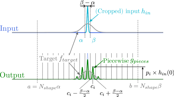
Figure S6: Notations in use for the shaping problem. A piecewise function $g_{pieces}$ is built by filling $N_{shape}$ bins (centered around the $c_{i}$) with $p_{i}$-weighted copies of an input profile $h_{in}$, so as to match a target shape $f_{target}$. $\beta-\alpha$ gives the width of the bins (see part E.4.2).

We further assume that the functions are $L^{2}$-normalised, that is

$$\int_{a}^{b}\left|f_{target}\right|{{}^{2}}(t)\mathrm{d}t=1=\int_{-\frac{b-a}{2N_{shape}}}^{\frac{b-a}{2N_{shape}}}\left|h_{in}\right|{{}^{2}}(t)\mathrm{d}t.$$ (136)

The shaped photon waveform is then represented by a continuous function $g_{pieces}\in\mathcal{C}_{0}([a,b]\rightarrow\mathbb{C})$. Subject to the constraint of it being normalised, we will look for a way to build a piecewise $g_{pieces}$ that maximises the overlap with $f_{target}$. We take $g_{pieces}$ split into pieces that are all weighted versions of profile $h_{in}$ with weights $0\leq p_{i}\leq 1$ and $0\leq\theta_{i}<2\pi$ phases ($i\in[[0,N_{bins}-1]]$), that is

$$g_{pieces}(t):=\sum_{j=0}^{N_{shape}-1}p_{j}e^{i\theta_{j}}\mathds{1}_{\left[c_{j}-\frac{b-a}{2N_{shape}},c_{j}+\frac{b-a}{2N_{shape}}\right]}(t)\times h_{in}(t-c_{j}).$$

We introduced the bins centers positions

$$\forall i\in[[0,N_{shape}-1]]\quad c_{i}:=\frac{b-a}{2N_{shape}}+i\frac{b-a}{N_{shape}}=\left(i+\frac{1}{2}\right)\frac{b-a}{2N_{shape}},$$

and $\mathds{1}$ stands for the indicatrix function.

We then want to optimise the objective functional

$$R_{f_{target}}(p,\theta,h_{in}) = \left|\int_{a}^{b}f_{target}(t)^{*}g_{pieces}(t)\mathrm{d}t\right|=\left|\sum_{j=0}^{N_{shape}-1}p_{j}e^{i\theta_{j}}{\int_{c_{j}-\frac{b-a}{2N_{shape}}}^{c_{j}+\frac{b-a}{2N_{shape}}}f_{target}(t)^{*}h_{in}(t-c_{j})\mathrm{d}t}\right|$$ (137)

subject to the normalisation constraint

$$\sum_{i=0}^{N_{shape}-1}p_{i}{{}^{2}}=1.$$ (138)

The normalisation constraint 138 ensures that

$$1 = \int_{a}^{b}\left|g_{pieces}\right|{{}^{2}}(t)\mathrm{d}t=\sum_{j=0}^{N_{shape}-1}p_{j}{{}^{2}}\int_{c_{j}-\frac{b-a}{2N_{shape}}}^{c_{j}+\frac{b-a}{2N_{shape}}}\left|h_{in}\right|{{}^{2}}(t-c_{j})\mathrm{d}t=\sum_{j=0}^{N_{shape}-1}p_{j}{{}^{2}}\times 1$$

since $h_{in}$ is normalised (Eq. 136). For convenience, we introduce the overlap $J_{j}^{f_{target},h_{in}}$ between the input translated to bin $j$ and the target restricted to that bin,

$$J_{j}^{f_{target},h_{in}}:=\int_{c_{j}-\frac{b-a}{2N_{shape}}}^{c_{j}+\frac{b-a}{2N_{shape}}}f_{target}(t)^{*}h_{in}(t-c_{j})\mathrm{d}t.$$ (139)

E.2 Optimal weights for the piecewise target

For a given arbitrary $h_{in}$, the optimal weights $(p_{i})$ can be found in the following way. $R_{f_{target}}(p,h_{in})$ with given $h_{in}$ is bounded by the Cauchy-Schwarz inequality on $\mathbb{C}^{N_{bins}}$

$$R_{f_{target}} = \left|\sum_{j=0}^{N_{shape}-1}p_{j}e^{i\theta_{j}}J_{j}^{f_{target},h_{in}}\right|$$

$$\leq \sqrt{\underset{=1\text{ by constraint}}{\underbrace{\left(\sum_{j=0}^{N_{shape}-1}p_{j}^{2}\right)}}\left(\sum_{j=0}^{N_{shape}-1}\left|J_{j}^{f_{target},h_{in}}\right|^{2}\right)},$$

and the two sides are equal if and only if the two vectors $\left(\left[p_{j}e^{i\theta_{j}}\right]^{*}\right)_{j\in[[0,N_{shape}-1]]}$ and $(J_{j}^{f_{target},h_{in}})_{j\in[[0,N_{shape}-1]]}$ are linearly dependant. Thus, the optimal normalised $(p_{j}^{opt})_{j}$ and $(\theta_{j}^{opt})_{j}$ are such that

$$\forall j\quad p_{j}^{opt}=\frac{\left|J_{j}^{f_{target},h_{in}}\right|}{\sqrt{\sum_{j=0}^{N_{shape}-1}\left|J_{j}^{f_{target},h_{in}}\right|^{2}}},$$ (141)

and

$$\forall j\quad\theta_{j}^{opt}=-\mathrm{Arg}\left(J_{j}^{f_{target},h_{in}}\right).$$ (142)

In this case, the value for the overlap 137 is

$$R_{f_{target}} = \left|\sum_{j=0}^{N_{shape}-1}\left[p_{j}^{opt}\right]^{*}e^{-i\theta_{j}^{opt}}J_{j}^{f_{target},h_{in}}\right|$$ (143)

$$= \frac{\sum_{j=0}^{N_{shape}-1}\left|J_{j}^{f_{target},h_{in}}\right|^{2}}{\sqrt{\sum_{j=0}^{N_{shape}-1}\left|J_{j}^{f_{target},h_{in}}\right|^{2}}}$$

$$= \sqrt{\sum_{j=0}^{N_{shape}-1}\left|J_{j}^{f_{target},h_{in}}\right|^{2}}.$$

Note that in the model, we fixed the position of the bin centers $c_{i}$. This position is actually not important for the limit $N_{shape}\rightarrow\infty$, but could be optimised for finite-size shaping. In particular, for small values of $N_{shape}$, one should change the bin centers for even and odd values of $N_{shape}$. However, for most situations where $N_{shape}>5$ the difference is not so big, as verified numerically. We thus keep that hypothesis, even if the position might require to be fine tuned manually.

E.3 Translation into partial readouts on the memory

The $(p_{i}^{2})_{i}$ are the absolute weights for the distribution of emission probabilities with $\sum_{i=0}^{N_{shape}-1}p_{i}{{}^{2}}=1$. As the pieces will be emitted sequentially, it is important to translate the $(p_{i})_{i}$ into relative weights $(q_{i})_{i}$ that indicate how much of the remaining amplitude is to be emitted at step $i$. Then those weights shall be converted into control parameters depending on what kind of impulsions are used to control emission from the memory.

E.3.1 Relative amplitudes chain

We look for a succession of impulsions to retrieve a proportion $q_{i}^{2}$ of the remaining amplitude for every step $i$, and keep $(1-q_{i}^{2})$.

By induction on $N_{shape}\geq 1$ we can show that for any $(q_{i})_{0\leq i\leq N_{bins}-1}$ such that $q_{N_{shape}-1}=1$ (requirement that the memory is empty after last pulse), we get

$$\sum_{i=0}^{N_{shape}-1}q_{i}^{2}\times\prod_{j<i}(1-q_{j}^{2})=1.$$

This gives the absolute amplitudes retrieved at every step, the $(p_{i})_{i}$, as a function of the relative amplitudes $(q_{i})_{i}$, namely

$$\begin{cases}p_{0}^{2}&=q_{0}^{2}\\ \forall i>0\quad p_{i}^{2}&=q_{i}^{2}\prod_{j<i}(1-q_{j}^{2})\end{cases}.$$

If the $(p_{i})_{i}$ are given and assumed non-zero, we can compute the $(q_{i})_{i}$ recursively as

$$\begin{cases}q_{0}^{2}&=p_{0}^{2}\\ q_{1}^{2}&=\frac{p_{1}^{2}}{(1-q_{0}^{2})}\\ &\vdots\\ q_{i}^{2}&=\frac{p_{i}^{2}}{\prod_{j<i}(1-q_{j}^{2})}\end{cases},$$

and obtain by induction an explicit conversion formula

$$\begin{cases}q_{0}^{2}&=p_{0}^{2}\\ \forall i>0\quad q_{i}^{2}&=\frac{p_{i}^{2}}{1-\sum_{j<i}p_{j}^{2}}\end{cases}.$$

Note that for every $i$, $q_{i}>p_{i}$ as expected. If there is an index $i$ such that $q_{i}=1$, then all the next weights will be zero.

E.3.2 Chain of $\pi$-pulses

The conversion of relative amplitudes $q_{i}$ into control amplitudes $\Omega_{i}$ for partial pulses shone onto the atoms depends on the type of control pulses. For rectangular pulses, the formula was given in Section B, and corresponds to Eq. 74. Furthermore, the optimal phase $\theta_{i}^{opt}$ (see Eq. 142) can be added to each control pulse. When dealing with real wavepackets no phase is required.

E.4 Suboptimal efficiency for infinite stretching

E.4.1 Insight from photon shaping

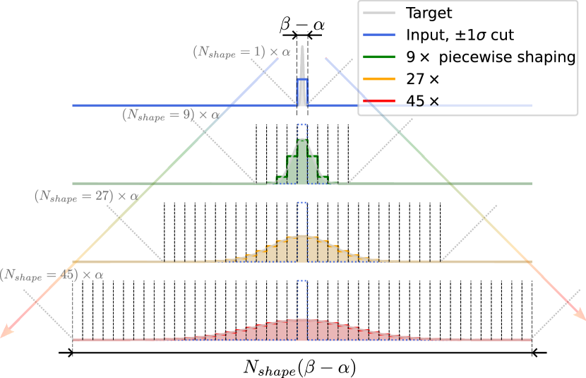
Figure S7: Instead of reducing the size of the pieces (rectangular here) used to build the piecewise approximations, we rather keep the input pieces constant and study how well they can be used to approximate a L²-normalised function $f_{target}$ with growing width (resp. $N_{shape}=9$, $27$ and $45$ stretching factors for green, orange and red curves w.r.t. the top grey Gaussian).

The previous description started from the definition of $f_{target}$ over $[a,b]$ and described the construction of a piecewise function $g_{pieces}$ from bins that are $N_{shape}$ subdivisions of $[a,b]$. The bins are filled by copies of $h_{in}$, the width of which is constrained by the bin size $\frac{b-a}{N_{shape}}$. From now on, we will rather take the perspective of a photon stretching procedure, where $h_{in}$ has a fixed temporal width over $[\alpha,\beta]$. The piecewise function $g_{pieces}$ is then made from $N_{shape}$ weighted copies of $h_{in}$. The aim is to set the weights to maximise the overlap with $f_{target}$ whose width can be increased (see Fig. S7).

E.4.2 Convergence towards infinity

We use our shaping scheme by carving a longer envelope with successive echoes. It turns out that when looking at the limit of a target much longer than the input, one gets an asymptotic value for the overlap. We hereby provide a proof for this limit, restricting to a case were we assume that $f_{target}$ is real-valued and that the input $h_{in}$ is real-valued and has a constant sign, let’s say positive. Thanks to this assumption, we can use the generalised mean value theorem to obtain that for every $j$, there exists a $\tau_{j}\in\left[c_{j}-\frac{b-a}{2N_{shape}};c_{j}+\frac{b-a}{2N_{shape}}\right]$ such that

$$J_{j}^{f_{target},h_{in}} = \int_{c_{j}-\frac{b-a}{2N_{shape}}}^{c_{j}+\frac{b-a}{2N_{shape}}}f_{target}(t)h_{in}(t-c_{j})\mathrm{d}t$$

$$= f_{target}(\tau_{j})\times\int_{c_{i}-\frac{b-a}{2N_{shape}}}^{c_{i}+\frac{b-a}{2N_{shape}}}h_{in}(t-c_{j})\mathrm{d}t$$

$$= f_{target}(\tau_{j})\times\int_{-\frac{b-a}{2N_{shape}}}^{+\frac{b-a}{2N_{shape}}}h_{in}(t)\mathrm{d}t$$

$$= f_{target}(\tau_{j})\times\frac{b-a}{N_{shape}}$$

$$\qquad\qquad\times\left(\frac{N_{shape}}{b-a}\int_{-\frac{b-a}{2N_{shape}}}^{+\frac{b-a}{2N_{shape}}}h_{in}(t)\mathrm{d}t\right)$$

$$=: f_{target}(\tau_{j})\times\frac{b-a}{N_{shape}}\times\hat{h}_{in}(0)$$

where we denote $\hat{h}_{in}(0)$ the mean value of $h_{in}$ over its support.

Then the optimal overlap from Eq. 143 involves a set of $(\tau_{j})_{j\in[0,N_{shape}-1]}$ where $\forall j\quad\tau_{j}\in\left[c_{j}-\frac{b-a}{2N_{shape}};c_{j}+\frac{b-a}{2N_{shape}}\right]$ such that

$$R_{f_{target}}^{opt}(p^{opt},h_{in})^{2} = \sum_{j=0}^{N_{shape}-1}\left|J_{j}^{f_{target},h_{in}}\right|^{2}$$

$$= \hat{h}_{in}(0)^{2}\times\left(\frac{b-a}{N_{shape}}\right)^{2}\times\sum_{j=0}^{N_{shape}-1}\left|f_{target}(\tau_{j})\right|^{2}$$

$$= \hat{h}_{in}(0)^{2}\times\frac{b-a}{N_{shape}}\times\sum_{j=0}^{N-1}\int_{c_{j}-\frac{b-a}{2N_{shape}}}^{c_{j}+\frac{b-a}{2N_{shape}}}\left|f_{target}(\tau_{j})\right|^{2}\mathrm{d}t.$$

Now, as illustrated in Fig. S7, we keep the width of $h_{in}$ constant, while the profile $f_{target}$ is stretched. As such, we take $a=N_{shape}\alpha$ and $b=N_{shape}\beta$ and $N_{shape}$ bins centered at $c_{i}$. We further define $c_{i}^{(0)}=\frac{c_{i}}{N_{shape}}$. Besides we define a reference profile $\psi:[\alpha,\beta]\rightarrow\mathbb{R}$ such that $\int_{\alpha}^{\beta}\psi^{2}=1$ and define a sequences of growing target profiles

$$f_{target,N_{shape}}: \left[N_{shape}\alpha;N_{shape}\beta\right]\rightarrow\mathbb{R}$$

$$t\mapsto\frac{1}{\sqrt{N_{shape}}}\psi\left(\frac{t}{N_{shape}}\right).$$

By means of a change of variables, one can check that $\forall N_{bins}\quad\int_{a=N_{shape}\alpha}^{b=N_{shape}\beta}f_{target,N_{shape}}^{2}=1$. We write $R_{N_{shape}}$ for the optimal overlap $R_{f_{target,N_{shape}}}^{opt}(p^{opt},h_{in})$ of Eq. E.4.2.

Let $\varepsilon>0$ and as $\psi^{2}$ is uniformly continuous over $[\alpha;\beta],$ let $\delta>0$ such that $\forall x,y\quad\left|x-y\right|\leq\delta\Rightarrow\left|\psi^{2}(x)-\psi^{2}(y)\right|\leq\varepsilon$. Then

$$\left|\sum_{i=0}^{N_{shape}-1}\int_{N_{shape}c_{i}^{(0)}-\frac{\beta-\alpha}{2}}^{N_{shape}c_{i}^{(0)}+\frac{\beta-\alpha}{2}}f_{target,N_{shape}}(\tau_{i})^{2}\mathrm{d}t-\int_{a=N_{shape}\alpha}^{b=N_{shape}\beta}f_{target,N_{shape}}(t)^{2}\mathrm{d}t\right|$$

$$= \frac{1}{N_{shape}}\left|\sum_{i=0}^{N_{shape}-1}\int_{N_{shape}c_{i}^{(0)}-\frac{\beta-\alpha}{2}}^{N_{shape}c_{i}^{(0)}+\frac{\beta-\alpha}{2}}\psi\left(\frac{\tau_{i}}{N_{shape}}\right)^{2}\mathrm{d}t-\int_{a=N_{bins}\alpha}^{b=N_{bins}\beta}\psi\left(\frac{t}{N_{shape}}\right)^{2}\mathrm{d}t\right|$$

$$\leq \frac{1}{N_{shape}}\sum_{i=0}^{N_{shape}-1}\int_{N_{shape}c_{i}^{(0)}-\frac{\beta-\alpha}{2}}^{N_{shape}c_{i}^{(0)}+\frac{\beta-\alpha}{2}}\left|\psi\left(\frac{\tau_{i}}{N_{shape}}\right)^{2}-\psi\left(\frac{t}{N_{shape}}\right)^{2}\right|\mathrm{d}t$$

$$\leq \frac{1}{N_{shape}}\sum_{i=0}^{N_{shape}-1}\int_{N_{shape}c_{i}^{(0)}-\frac{\beta-\alpha}{2}}^{N_{shape}c_{i}^{(0)}+\frac{\beta-\alpha}{2}}\varepsilon\mathrm{d}t$$

$$= \frac{1}{N_{shape}}\times N_{shape}\times(\beta-\alpha)\times\varepsilon,$$

where the first inequality stems from triangular inequality, and the last inequality holds if $N_{shape}$ is big enough (in that case $\left|\frac{\tau_{i}}{N_{shape}}-\frac{t}{N_{shape}}\right|\leq\frac{\beta-\alpha}{N_{shape}}\leq\delta$). As such, if $N_{shape}$ is big enough one gets

$$\left|\frac{1}{\hat{h}_{in}(0)^{2}(\beta-\alpha)}R_{N_{shape}}^{2}-\int_{\alpha}^{\beta}\psi(t)^{2}\mathrm{d}t\right|=\left|\sum_{i=0}^{N_{shape}-1}\int_{c_{i}^{(0)}-\frac{\beta-\alpha}{2N_{shape}}}^{c_{i}^{(0)}+\frac{\beta-\alpha}{2N_{shape}}}f_{target}(\tau_{i})^{2}\mathrm{d}t-\int_{a=N_{shape}\alpha}^{b=N_{shape}\beta}f_{target,N_{shape}}(t)^{2}\mathrm{d}t\right|\leq\varepsilon.$$

That is, as we consider positive quantities

$$R_{N_{shape}}\xrightarrow[N_{shape}\rightarrow+\infty]{}\sqrt{\beta-\alpha}\times\underset{=\hat{h}_{in}(0)}{\underbrace{\left(\frac{1}{\beta-\alpha}\int_{\alpha}^{\beta}h_{in}(t)\mathrm{d}t\right)}}\times\underset{=1}{\underbrace{\sqrt{\int_{\alpha}^{\beta}\psi(t)^{2}\mathrm{d}t}}}=\frac{1}{\sqrt{\beta-\alpha}}\int_{\alpha}^{\beta}h_{in}(t)\mathrm{d}t.$$ (145)

To sum up, when $N_{shape}\rightarrow\infty$, the overlap $R_{N_{shape}}$ has a limit which only depends on the memory input $h_{in}$ (also assumed to be the unshaped output) and not on $f_{target}$. From the left-hand side of equality 145, we see that, given a bin size $(\beta-\alpha)$, the limit of the overlap is optimal when the mean value of the input profile $h_{in}$ is maximised. From Cauchy-Schwarz inequality, this corresponds to $h_{in}:t\mapsto\frac{1}{\sqrt{\beta-\alpha}}$, and then $R_{N_{shape}}\rightarrow 1$. However, the shape $h_{in}$ is usually given before the shaping. As it is studied in paragraph E.4.3, the optimisation is rather to be done on the choice of $\alpha$ and $\beta$.

Moreover, it turns out that the convergence 145 is quite fast. As expected for Riemann-sum-like results, it actually goes as $\frac{1}{N_{shape}^{2}}$. We observe numerically that for targets about $10$ times longer than the input, the overlap is already less than $1$ % away from the theoretical limit.

As a side remark, we conjecture that a similar result stands when a real-valued $h_{in}$ does not keep a constant sign, by focusing on different slices of its natural domain where it does. Moreover, we point out that our proof was inspired by demonstrations of Riemann-Lebesgue lemma and Fejér’s theorem [84, 85], that might also provide a more direct way to the result. From this perspective, $g_{pieces}$, a weighted regular juxtaposition of $h_{in}$ kernels, appears as a modulated periodic function, that somehow samples the wider $f_{target}$ as a comb of identity approximations when $N_{shape}\rightarrow\infty$.

E.4.3 Optimisation of the limit: cropped-echo technique

We now allow $\int_{\alpha}^{\beta}h_{in}(t)^{2}\mathrm{d}t\leq 1$ by defining $h_{in}$ as a L²-normalised function over a broader support $[\alpha^{\prime};\beta^{\prime}]$, and cutting it between $\alpha$ and $\beta$ (that is $\alpha^{\prime}\leq\alpha<\beta\leq\beta^{\prime}$) so as to maximise the quantity $\frac{1}{\sqrt{\beta-\alpha}}\int_{\alpha}^{\beta}h_{in}(t)\mathrm{d}t$. This is what we call the cropped-echo technique. For instance, let us take $\alpha^{\prime}\rightarrow-\infty$ and $\beta^{\prime}\rightarrow+\infty$ and consider a L²-normalised Gaussian over $\mathbb{R}$ with standard deviation $\sigma$ (that is fixed). Then we choose $\alpha=-M\sigma$ and $\beta=M\sigma$ with a varying width ratio $M$ to define $h_{in}$ as the restriction of Gaussian to $[\alpha,\beta]$ (thus not normalised), as illustrated in Fig. S8. The resulting overlap limit 145 related to the cut of this Gaussian is

$$\frac{1}{\sqrt{2M\sigma}}\int_{-M\sigma}^{M\sigma}\frac{1}{(\pi\sigma^{2})^{1/4}}e^{-t^{2}/2\sigma^{2}}\mathrm{d}t = \frac{1}{\pi^{1/4}\sqrt{2M}\sigma}\times\sqrt{2}\sigma\int_{-M/\sqrt{2}}^{M/\sqrt{2}}e^{-u^{2}}\mathrm{d}u\text{ with the change of variables $u=\frac{t}{\sigma\sqrt{2}}$}$$ (146)

$$= \frac{1}{\pi^{1/4}\sqrt{M}}\times\sqrt{\pi}\times\frac{2}{\sqrt{\pi}}\int_{0}^{M/\sqrt{2}}e^{-u^{2}}\mathrm{d}u$$

$$= \frac{\pi^{1/4}}{\sqrt{M}}\mathrm{erf}\left(\frac{M}{\sqrt{2}}\right),$$

which is represented in Fig. S9. It is seen that the overlap is optimal around $M\approx 1.4$, reaching about $0.94$. For an exponential input, $h_{in}:t\mapsto\sqrt{2}e^{-t}\mathds{1}_{x\geq 0}$, and truncation between $\alpha=0$ and $\beta=M$, we obtain the truncation value limit 145 $\sqrt{\frac{2}{M}}(1-e^{-M})$. The optimal value is about $0.9$, found for $M\approx 1.26$.

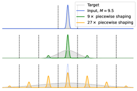
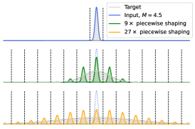
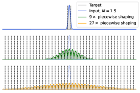
Figure S8: For a Gaussian input profile (in blue on top), we apply different cutoff factors ($M=9.5$, $4.5$ and $1.5$ from left to right, bins are delimited by the dashed vertical black lines) to define the piece $h_{in}$ used to build the piecewise function $g_{pieces}$ (in green and in orange) that is used to match the target $f_{target}$ (in grey) using optimal coefficients from Eq. 141. This $f_{target}$ is a L²-normalised Gaussian function chosen $9$ times (middle) or $27$ times (bottom) as wide as the initial uncropped Gaussian input.

Crucially, we note that the cropped-echo technique gives nice results on AFC simulations, as illustrated in the main text. In this section, the mathematical formulation dealt with independent time bins of weighted copies of $h_{in}$. When implementing that on an AFC quantum memory, the late cropped-part of an echo readout stays in the memory and may interfere with later partial readouts and thus change the shape of the resulting echoes. Such interferences could be observed, but did not happen to be detrimental to the efficiencies.

Finally, we recall that in Fig. 3 of the main text, we evaluate the efficiency of the shaping process in two steps. First, the loss of energy is considered, as it matters for the whole network entanglement generation rate (see Appendix A). In our mathematical context, loss of energy due to the memory (see Eq. B.2.3) can also be taken into account with some undernormalised $h_{in}$. The losses due to the left and right crops are $\int_{-\infty}^{-M\sigma}\left|h_{in}(t)\right|^{2}\mathrm{d}t$ and $\int_{M\sigma}^{+\infty}\left|h_{in}(t)\right|^{2}\mathrm{d}t$. Second, the overlap with the target shape is taken renormalised with respect to the losses, that is by considering

$$\int\frac{\mathcal{E}_{out}}{\sqrt{\eta_{out}}}\cdot f_{target}^{*},$$

where $\eta_{out}$ gives the total energy of the shaped echo (integral bounds defined accordingly). In our context, $\mathcal{E}_{out}$ corresponds to $g_{pieces}$ and $\eta_{out}$ is given by

$$\int_{a}^{b}\left|g_{pieces}\right|{{}^{2}}(t)\mathrm{d}t=\sum_{j=0}^{N_{shape}-1}p_{j}{{}^{2}}\int_{c_{j}-M\sigma}^{c_{j}+M\sigma}\left|h_{in}\right|{{}^{2}}(t-c_{j})\mathrm{d}t=\int_{-M\sigma}^{M\sigma}\left|h_{in}\right|{{}^{2}}(t)\mathrm{d}t,$$ (147)

so that the renormalised asymptotic overlap 145 in the Gaussian case is

$$\frac{1}{\sqrt{\int_{-M\sigma}^{M\sigma}\left|\frac{1}{(\pi\sigma^{2})^{1/4}}e^{-t^{2}/2\sigma^{2}}\right|^{2}\mathrm{d}t}}\times\frac{\pi^{1/4}}{\sqrt{M}}\mathrm{erf}\left(\frac{M}{\sqrt{2}}\right) = (\pi\sigma^{2})^{1/4}\frac{1}{\sqrt{\sigma}\pi^{1/4}\sqrt{\mathrm{erf}\left(M\right)}}\times\frac{\pi^{1/4}}{\sqrt{M}}\mathrm{erf}\left(\frac{M}{\sqrt{2}}\right)$$ (148)

$$= \pi^{1/4}\times\frac{\mathrm{erf}\left(\frac{M}{\sqrt{2}}\right)}{\sqrt{M\mathrm{erf}\left(M\right)}}.$$

This renormalised overlap matters for the fidelity of the entanglement generated by the whole network (again, see Appendix A). Both quantities 147 and 148 are plotted in Fig. S9. The former increases monotonously with $M$, while latter seems to decrease monotonously with $M$, and has the limit $1$ when $M$ goes to $0$. A nice trade-off the two turns out to be given by the optimal value of the non-renormalised overlap 146. For $M\approx 1.4$, the remaining energy is about $0.95$ so that the renormalised overlap is almost $0.97$. Realistic AFC simulation outputs are consistent but slightly different from these values, as shown in Fig. 3 of the main text.

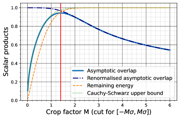
Figure S9: For Gaussian input profiles, the predicted asymptotic overlaps (Eq. 146 in blue, and renormalised 148 in deep blue, dash-dotted) are plotted as a function of the crop factor $M$. The non-renormalised overlap features an optimum slightly below $M\approx 1.4$ (vertical red line), about $94\%$. The Cauchy-Schwarz upper-bound $\left|\frac{1}{\beta-\alpha}\int_{\alpha}^{\beta}h_{in}(t)\times 1\mathrm{d}t\right|\leq\sqrt{\int_{\alpha}^{\beta}h_{in}(t)^{2}\mathrm{d}t}$ is given by the green dotted line. The remaining energy after crop $\int_{\alpha}^{\beta}h_{in}(t)^{2}\mathrm{d}t$ is given by the orange dashed line. At the former optimal point, one still finds $95\%$ of the initial energy in the cut profile.

Appendix F Coherence of pure single-photon state output

We showed in Section B.2.2 that, in the impedance-matching regime, the full device efficiency of the cavity-assisted AFC can reach $\eta_{1st-echo}=1$ (cf. Eq. B.2.3). In Section E, we argued that a purposefully chosen sequence of partial readouts results in a reshaping of the photon wavepacket, with a high efficiency. On top of that efficiency and that shape, we are interested in the properties of the output photon. Namely, we would like to make sure that purity is preserved, i.e. the quantum state of light emitted by the memory, after a pure single-photon state was absorbed, can be described by a pure single-photon state, at least conditioned on success of reemission. Such an outcome is expected since getting the post-selected state does not involve tracing over an environment of any kind. As such, we give a technique to retrieve the coherent state description from the resolutions of the memory Heisenberg equations, as done in Appendix D and Section D.4.

F.1 Need for a quantum state description

To start with, we underline that for our model, derivations could have been performed in the Schrödinger picture, by considering the evolution of state coordinates with time. For similar systems of equations, especially leveraging the one-excitation limit, it is for instance done in Refs. [66, 86, 87, 15, 88]. However, we chose so far to solve a set of Heisenberg-Langevin equations in the Heisenberg picture, as it seems to be the natural framework for introducing input-output relations as well as effects of quantum noise and damping. In the context of this Letter, we also seek to compute interferometric quantities that would involve both the photon coming from the memory and from an ion node in the full network of Fig. 1 in the main text. For the ion, and for the Hong-Ou-Mandel experiment presented in Sec. I, a description in terms of quantum states rather than quantum operators was used in the Literature [24, 18]. Hence, we shall find a way of translating our previous derivations that dealt with quantum operators into a Schrödinger–like description of the output photon in terms of quantum state.

F.2 Extracting a quantum state description from the Heisenberg picture

In the Heisenberg picture, the state of the whole system is not meant to change: only operators evolve with time. Still, the interaction between the input photon and the memory can be regarded as a scattering process [89, 45, 90, 91]. Describing the output state then amounts to factorising the Hilbert space in another way and to performing a change of basis. We start at time $t_{0}$ with the decomposition between the memory (cavity and atoms), the light environment (modes that carry a possible incoming photon) and the other reservoirs (baths for quantum noise) as

$$\mathcal{H}=\mathcal{H}_{mem}(t_{0})\otimes\mathcal{H}_{light-env}(t_{0})\otimes\mathcal{H}_{baths}(t_{0}).$$ (149)

In the Schrödinger picture, evolution happens from time $t_{0}$ to $t_{f}$ within the zero and one-excitation eigenspaces of the total number operator $\hat{N}_{tot}$ (cf. Eq. 31), while in the Heisenberg picture a convenient basis to describe the (initial at time $t_{0}$) state of the system is

$$\mathcal{B}_{t_{0}}:=\left\{\hat{\mathcal{E}}^{\dagger}(t_{0})|0\rangle\right\}\cup\left\{\hat{P}_{k}^{\dagger}(t_{0})|0\rangle,\hat{S}_{k}^{\dagger}(t_{0})|0\rangle\right\}_{1\leq k\leq N}\cup\left\{\hat{\mathcal{E}}_{in}^{\dagger}(t)|0\rangle\right\}_{t\in\mathbb{R}}\cup\left\{\hat{F}_{P,k}^{\dagger}(t)|0\rangle\right\}_{1\leq k\leq N,t\in\mathbb{R}}\cup\left\{\hat{F}_{S,k}^{\dagger}(t)|0\rangle\right\}_{1\leq k\leq N,t\in\mathbb{R}},$$ (150)

where $|0\rangle$ is again the vacuum state shared by all the subsystems. Note that we include all the set of quantum noise operators to take into account the excitations that would be within the reservoirs at time $t_{0}$. As detailed in Sec. C, the label $t$ in the noise operators does not refer to any time evolution but rather to a change of basis in the description of the bath modes. For example, the light environment is either fully described by the set of free space modes at time $t_{0}$ $\hat{c}_{light-env}(\omega,t_{0})^{\dagger}$ for all frequencies $\omega$, or by the set of input modes $\hat{\mathcal{E}}_{in}(t)=-\frac{i}{\sqrt{2\pi}}\int e^{-i\omega(t-t_{0})}\hat{c}_{light-env}(\omega,t_{0})\mathrm{d}\omega$ for all times $t$. The input state is defined within this basis, and typically

$$\rho_{ph,input} = |0\rangle_{mem}\langle 0|\otimes\left(\iint\mathcal{E}_{in}(t)\mathcal{E}_{in}^{*}(t^{\prime})\hat{\mathcal{E}}_{in}^{\dagger}(t)|0\rangle_{light-env}\langle 0|\hat{\mathcal{E}}_{in}(t^{\prime})\mathrm{d}t\mathrm{d}t^{\prime}\right)\otimes|0\rangle_{baths}\langle 0|$$ (151)

$$= \iint\mathcal{E}_{in}(t)\mathcal{E}_{in}^{*}(t^{\prime})\hat{\mathcal{E}}_{in}^{\dagger}(t)|0\rangle\langle 0|\hat{\mathcal{E}}_{in}(t^{\prime})\mathrm{d}t\mathrm{d}t^{\prime}=:|\psi_{input}\rangle\langle\psi_{input}|,$$

as discussed for Eq. 39 and paragraph D.4.3.

In order to represent the whole system standing at $t_{f}$ after interaction, we rather use the more suitable basis

$$\mathcal{B}_{t_{f}}:=\left\{\hat{\mathcal{E}}^{\dagger}(t_{f})|0\rangle\right\}\cup\left\{\hat{P}_{k}^{\dagger}(t_{f})|0\rangle,\hat{S}_{k}^{\dagger}(t_{f})|0\rangle\right\}_{1\leq k\leq N}\cup\left\{\hat{\mathcal{E}}_{out}^{\dagger}(t)|0\rangle\right\}_{t\in\mathbb{R}}\cup\mathcal{B}_{bath,t_{f}},$$ (152)

where we include the memory operators at time $t_{f}$, the light environment operators $\hat{\mathcal{E}}_{out}^{\dagger}(t)$ for all labels $t$ (or equivalently mode operators $\hat{c}_{light-env}^{\dagger}(\omega,t_{f})$ for all frequencies $\omega$) and a suitable basis build from other baths creation operators at time $t_{f}$. This change in representations amounts to a formal refactorisation of the Hilbert space 149 as

$$\mathcal{H}=\mathcal{H}_{mem}(t_{f})\otimes\mathcal{H}_{light-env}(t_{f})\otimes\mathcal{H}_{baths}(t_{f}).$$ (153)

Once the stance of decomposition from Eq. 152 is taken, the state of the output photon alone is obtained by tracing out other degrees of freedom (the memory and the other reservoirs). From basis $\mathcal{B}_{t_{f}}$, it corresponds to tracing out along all basis vectors except the set $\left\{\hat{\mathcal{E}}_{out}^{\dagger}(t)|0\rangle\right\}_{t\in\mathbb{R}}$. It is then clear that a suitable description for the photon state is

$$\rho_{ph,output} := \mathrm{Tr}_{\mathcal{B}_{t_{f}}(mem,baths)}(\rho_{ph,input})$$

$$= (1-\eta_{out})|0\rangle\langle 0|+\eta_{out}\rho_{out},$$

where $\eta_{out}$ is the efficiency that embraces all possible retrieval times and and $\rho_{out}$ is a normalised density matrix that is described in the subspace generated by the output states $\left\{\hat{\mathcal{E}}_{out}^{\dagger}(t)|0\rangle\right\}_{t\in\mathbb{R}}$ only. The vacuum component in the mixed state F.2 is a consequence of the fact that we work in the one-excitation subspace: the excitation is always present in the whole system, be that in the output field, or in the other parts (memory or other reservoirs). The latter are the ones that contribute to the vacuum component. As such, $\rho_{out}$ is obtained from the order-two correlators of output field operators of Sec. D.4, namely

$$\eta_{out}\rho_{out} = \iint\langle 0|\mathcal{\hat{E}}_{out}(t^{\prime})\rho_{ph,output}\hat{\mathcal{E}}_{out}^{\dagger}(t)|0\rangle\mathcal{\hat{E}}_{out}^{\dagger}(t)|0\rangle\langle 0|\mathcal{\hat{E}}_{out}(t^{\prime})\mathrm{d}t\mathrm{d}t^{\prime}$$ (155)

$$= \iint\mathrm{Tr}\left(\mathcal{\hat{E}}_{out}^{\dagger}(t)\hat{\mathcal{E}}_{out}(t^{\prime})\rho_{ph,input}\right)\mathcal{\hat{E}}_{out}^{\dagger}(t)|0\rangle\langle 0|\mathcal{\hat{E}}_{out}(t^{\prime})\mathrm{d}t\mathrm{d}t^{\prime}$$

$$= \iint\mathcal{E}_{out}^{*}(t)\mathcal{E}_{out}(t^{\prime})\mathcal{\hat{E}}_{out}^{\dagger}(t)|0\rangle\langle 0|\mathcal{\hat{E}}_{out}(t^{\prime})\mathrm{d}t\mathrm{d}t^{\prime}$$

where we used the fact that we work within the one-excitation subspace to go from the first equality to the second one, which in turn corresponds to Eq. 135 of Sec. D and uses the hypothesis of an initially empty memory as in Eq. 151. Hence, $\rho_{out}$ has the structure of a pure state in the output flying qubit basis so we write

$$\rho_{ph,output}=(1-\eta_{out})|0\rangle\langle 0|+\eta_{out}|\psi_{output}\rangle\langle\psi_{output}|,$$ (156)

and $|\psi_{out}\rangle$ has the temporal waveform $t\mapsto\mathcal{\mathcal{E}}_{out}(t)$ over output modes $\hat{\mathcal{E}}_{out}^{\dagger}$, i.e.

$$|\psi_{output}\rangle=\frac{1}{\sqrt{\eta_{out}}}\int\mathcal{E}_{out}(t)\hat{\mathcal{E}}_{out}^{\dagger}(t)|0\rangle\mathrm{d}t.$$ (157)

Finally, Eq. 157 shows that $\eta_{out}$ is obtained from the scalar equations by computing

$$\eta_{out}=\int\left|\mathcal{E}_{out}(t)\right|^{2}\mathrm{d}t.$$ (158)

According to this result, the whole conditional output mode is pure. In particular, the coherence spans over the first reflection and the later echoes. Similarly, the shaping process that involves partial control pulses keeps the purity, as long as the control pulses are coherent with one another. Moreover, the dephasing losses (rates $\gamma_{P}$ and $\gamma_{S}$) only affect the efficiency of the whole process and do not break the coherence of the output photon. On the contrary, they rather increase the value of $\eta_{out}$.

Appendix G Experimental parameters

In this Section, we explain how the memory parameters used in the main text were chosen. More precisely, we provide a way of translating our model parameters such as $g\sqrt{N}$,$\kappa$ and $\Gamma$ into quantities that can be assessed and measured experimentally. Some connections with the notations of some references that introduce similar models are also discussed. We summarise our choices in Table 3.

Parameters	Designation	Value	Reference
Cavity decay rate	$\kappa$	$2\pi\times 55\mathrm{MHz}$	Eq. 162
Inhomogeneous width	$\Gamma$	$2\pi\times 4$ MHz	Eq. 170
Collective coupling	$g\sqrt{N}$	$2\pi\times 8.4$ MHz (corresponds to $\tilde{d}=0.45$ in free space)	Eq. 174
Number of teeth	$N_{teeth}$	$67$	Eq. 175
Comb step	$\Delta$	$2\pi\times 61$ kHz	Eq. 176
Tooth width	$\gamma_{tooth}$	$2\pi\times 1$ kHz	Eq. 177
Optical transition decay	$\gamma_{P}$	$0$	Eq. 178
Spin transition decay	$\gamma_{S}$	$0$	Eq. 178

Table 3: Parameters chosen to feed the model, based on achievable experimental values.

G.1 Frequency units

First, we stress that by convention it is understood that parameters such as $\kappa$, $\Gamma$ and $g\sqrt{N}$ are given in $\mathrm{rad.s^{-1}}$. As such, the value in $\mathrm{rad.s^{-1}}$ is equal to the value in $\mathrm{Hz}$ multiplied by $2\pi$. We will consistently highlight the latter factor, by writing for instance $\Gamma=2\pi\times 4$ MHz to refer to the value in $\mathrm{rad.s}^{-1}$ ($25$ $\mathrm{rad.s}^{-1}$ approximately).

Depending on the references, some values can be found in both units and one should make sure that the right conversion is made. For instance in Ref. [35], the comb frequencies are given in $\mathrm{MHz}$, with echo time expressed as $\frac{1}{\Delta}$ where we recall that $\Delta$ is the distance between two comb teeth. We rather consider all frequencies in $\mathrm{rad.s^{-1}}$ so that the memory recurrence time is given by $\frac{2\pi}{\Delta}$.

Note that even if $\kappa$ refers to some decay rate of the cavity, for which an expression in $\mathrm{Hz}$ would seem natural, it is the value in $\mathrm{rad.s^{-1}}$ which is used in the relation with cavity finesse (see Eq. 159), as mentioned in Ref. [33].

G.2 Cavity finesse and decay rate

For a one-sided cavity (left mirror with reflectivity $R_{1}\lesssim 1$ and perfect right mirror with $R_{2}=1$) of length $L_{cav}$, the cavity finesse is defined as

$$\mathcal{F}_{cav} :=\frac{\Delta\omega_{FSR}}{\Delta\omega_{FWHM}}$$ (159)

$$=\frac{\pi}{2}\frac{1}{\mathrm{Arcsin}\left(\frac{1-\sqrt{R_{1}}}{2R_{1}^{1/4}}\right)}\approx\frac{\pi R_{1}^{1/4}}{1-\sqrt{R_{1}}},$$

where $\Delta\omega_{FSR}=\frac{\pi c}{L_{cav}}$ is the Fabry-Perot resonator free-spectral range [92], and $\Delta\omega_{FWHM}$ the FWHM of its transmission peaks. The field intensity decays with a rate $-\frac{\ln(R_{1})}{2L_{cav}/c}$ per cavity round-trip, so that we define the field amplitude decay rate $\kappa$ as half that quantity

$$\kappa\approx\frac{c}{4L_{cav}}(1-R_{1}).$$ (160)

As such, the “lifetime” of a photon within the cavity is $\frac{1}{2\kappa}$, and the “the number of passes a photon would make through an empty cavity before leaking out” is $\frac{1}{2\kappa}\times\frac{c}{L_{cav}}\approx\frac{\mathcal{F}}{\pi}$ [39]. Expanding $\mathcal{F}_{cav}$ and $\kappa$ in terms of $\ln(R_{1})$ for small values of $1-R_{1}$ leads to the approximation

$$\mathcal{F}_{cav}\approx\frac{\pi c}{2L_{cav}\kappa}=\frac{\Delta\omega_{FSR}}{2\kappa},$$ (161)

which is sometimes taken as a definition.

In Refs. [35], the cavity is chosen such that $R_{1}=0.4$ and $R_{2}=0.97$. This yields $\mathcal{F}_{cav}\approx 6.5$ as mentioned in the text. In addition, the cavity has a length $L_{cav}=208$ mm, so that

$$\kappa=3.4\times 10^{8}\text{ }\mathrm{rad.s^{-1}}=2\pi\times 55\text{ MHz}.$$ (162)

This last value can also be obtained from the values of the free spectral range $\Delta\omega_{FSR}=2\pi\times 7.2\times 10^{8}$ MHz and the cavity linewidth $\gamma_{cav}=\frac{\Delta\omega_{FSR}}{\mathcal{F}_{cav}}=2\pi\times 111$ MHz.

Note that in the experiment of Refs. [73, 35] the vacuum chamber with the crystal is mounted between the two cavity mirrors, which leads to losses due to reflections on the chamber windows. These losses impact every round-trip. Note that we did not include these intra-cavity losses in our model.

G.3 Comb structure and optical depth

G.3.1 Probing the transmission profile

A standard way to evaluate the atomic density within a crystal is to perform a transmission experiment. Typically, one shines a probe continuous laser at frequency $\xi$ through the crystal (without any cavity), and the measured transmission curve $T(\xi)$ can be used to extract the optical density of the crystal as a function of $\xi$ (see for instance Fig. 1.c) in Ref. [35]).

To describe such an experiment without any cavity, Maxwell-Bloch or related Heisenberg-Langevin equations in free space must be introduced instead of system 32, as it is done in Refs. [40, 62, 30, 93] for instance. In the envelope approximation [61], one can write propagation along an axis with $z$ coordinate as

$$\begin{cases}\partial_{t}\mathcal{E}(z,t)+c\partial_{z}\mathcal{E}(z,t)&=igN\int n(\omega)\sigma_{\omega}(z,t)\mathrm{d}\omega\\ \hfill\partial_{t}\sigma_{\omega}(z,t)&=-i\omega\sigma_{\omega}(z,t)+ig\mathcal{E}(z,t),\end{cases}$$ (163)

where $\int n(\omega)\mathrm{d\omega}=1$ gives the atomic distribution normalisation, $N$ the total number of atoms that interact with the field, and $\sigma_{\omega}$ the collective polarisation for frequency classes around detuning $\omega$. Note that no damping is included here.

To solve this quickly, we will use rough notations of Fourier transforms and distribution theory, with a convention where the plane waves involve $e^{-i\xi t}$: $f(t)=\int\hat{f}(\xi)e^{-i\xi t}\mathrm{d}\xi$ ($\xi$ is understood as the angular frequency in $\mathrm{rad.s}^{-1}$). Taking the Fourier transform $t\leftrightarrow\xi$ of the equations yields

$$\begin{cases}-i\xi\hat{\mathcal{E}}(z,\xi)+c\partial_{z}\mathcal{\hat{\mathcal{E}}}(z,\xi)&=igN\int n(\omega)\hat{\sigma}_{\omega}(z,\xi)\mathrm{d}\omega\\ -i\xi\hat{\sigma}_{\omega}(z,\xi)&=-i\omega\hat{\sigma}_{\omega}(z,\xi)+ig\mathcal{\hat{\mathcal{E}}}(z,\xi),\end{cases}$$

which is

$$\begin{cases}\hat{\sigma}_{\omega}(z,\xi)&=\frac{g}{\omega-\xi}\hat{\mathcal{E}}(z,\xi)\\ \partial_{z}\mathcal{\hat{\mathcal{E}}}(z,\xi)&=-i\frac{\xi}{c}\hat{\mathcal{E}}(z,\xi)+i\frac{g^{2}N}{c}\left(\int_{\mathbb{R}}\frac{n(\omega)}{\omega-\xi}\mathrm{d}\omega\right)\hat{\mathcal{E}}(z,\xi).\end{cases}$$

The last equation is solved with an exponential; the imaginary part of the argument yields the decay rate of the field amplitude as a function of $z$. In particular, one gets for the field intensity

$$\partial_{z}\left|\mathcal{\hat{\mathcal{E}}}(z,\xi)\right|^{2}=+i\frac{2g^{2}N}{c}\mathrm{Im}\left(\int_{\mathbb{R}}\frac{n(\omega)}{\omega-\xi}\mathrm{d}\omega\right)\left|\mathcal{\hat{\mathcal{E}}}(z,\xi)\right|^{2}$$ (164)

The integral can be computed using Kramers-Kronig relations (or Sokhotski-Plemelj theorem) stemming from complex analysis. If $n$ is a continuous function on the real line, one gets for the imaginary part (below, we don’t need the dispersive part of the equation)

$$n(\xi)=\frac{1}{i\pi}\mathrm{v.p.}\int_{\mathbb{R}}\frac{n(\omega)}{\omega-\xi}\mathrm{d}\omega$$ (165)

with v.p. denoting the Cauchy principal value of the integral. Thus Eq. 164 becomes a Beer Lambert–like equation [94]

$$\partial_{z}\left|\mathcal{\hat{\mathcal{E}}}(z,\xi)\right|^{2}=-\frac{2\pi g^{2}N}{c}n(\xi)\left|\mathcal{\hat{\mathcal{E}}}(z,\xi)\right|^{2},$$ (166)

which is solved as

$$\left|\mathcal{\hat{\mathcal{E}}}(z,\xi)\right|^{2}=e^{-\frac{2\pi g^{2}N}{c}n(\xi)z}\left|\mathcal{\hat{\mathcal{E}}}(0,\xi)\right|^{2}.$$

So the single pass transmission at frequency $\xi$ is given by

$$T(\xi)=\frac{\left|\mathcal{\hat{\mathcal{E}}}(z=L_{crys},\xi)\right|^{2}}{\left|\mathcal{\hat{\mathcal{E}}}(z=0,\xi)\right|^{2}}=e^{-\frac{2\pi g^{2}N}{c}n(\xi)L_{crys}},$$

where we note $L_{crys}$ for the crystal sample length along $z$-axis.

The optical depth is defined with the natural logarithm of the transmittance for laser detuning $\omega$ (formerly $\xi$),

$$\mathrm{OD}(\omega):=-\ln T(\omega)=\frac{2\pi g^{2}N}{c}n(\omega)L_{crys}.$$ (167)

So, in this undamped case, the optical depth is found to be proportional to the atomic distribution $n$. As such, it is understood that if one shines a continuous laser at frequency $\omega$ through the crystal, the measured absorbance curve $T(\omega)$ can be used to extract the optical density as a function of $\omega$. We can also define the absorption coefficient $\alpha(\omega)$ such that $\mathrm{OD}(\omega)=\alpha(\omega)L_{crys}$: $\alpha(\omega)=\frac{2\pi g^{2}N}{c}n(\omega)$, as used in Refs. [69, 95, 71]

G.3.2 Mean optical depth $\tilde{d}$

What is more, we can solve system 163 with the same tricks as for the cavity case, first by integrating

$$\sigma_{\omega}(t)=e^{-i\omega(t-t_{0})}\sigma_{\omega}(t_{0})+ig\int_{t_{0}}^{t}e^{-i\omega(t-t^{\prime})}\mathcal{E}(z,t^{\prime})\mathrm{d}t^{\prime}$$

and inserting that result into the equation for $\mathcal{E}(z,t)$ where we neglect temporal variations, which yields

$$\frac{\partial\mathcal{E}}{\partial z}(z,t) = -\frac{g^{2}N}{c}\int_{t_{0}}^{t}\tilde{n}(t-t^{\prime})\mathcal{E}(z,t^{\prime})\mathrm{d}t^{\prime}$$

$$+i\frac{gN}{c}\int e^{-i\omega(t-t_{0})}\sigma_{\omega}(t_{0})\mathrm{d}\omega.$$

Absorption only involves the central peak of $\tilde{n}(t)$ (as for Eq. 57) and if we assume that the atomic ensemble is initially empty ($\sigma_{\omega}(t_{0})=0$) we get

$$\frac{\partial\mathcal{E}}{\partial z}(z,t\approx t_{0})\approx-\frac{g^{2}N}{c}\frac{D_{comb}}{2}\mathcal{E}(z,t).$$

The mean absorption coefficient per unit length of a light pulse in the AFC structure can be introduced as

$$\frac{\tilde{\alpha}}{2}=\frac{g^{2}ND_{comb}}{2c},$$

and the mean optical density as

$$\tilde{d}=\tilde{\alpha}L_{crys}=\frac{g^{2}ND_{comb}}{c}L_{crys}.$$ (168)

$\tilde{d}$ corresponds to the absorption power of the inhomogeneous ensemble without the teeth.

Now recall from Eqs. 44 and 45 that we wrote the AFC atomic distribution as

$$n(\omega)\approx\frac{\Delta}{\int w(\omega)\mathrm{d}\omega\times\int v(\omega)\mathrm{d}\omega}\times v(\omega)\times\sum_{n=-\infty}^{+\infty}w(\omega-n\Delta),$$ (169)

with $w(0)=v(0)=1$ (see Table 2). Consider the maximal value $d_{max}=\mathrm{OD}(0)$ reached by the central peak of the optical density, that we also call the peak optical depth. From Eq. 167, it is linked to $n(0)=\frac{\Delta}{\int w(\omega)\mathrm{d}\omega\times\int v(\omega)\mathrm{d}\omega}=\frac{\Delta}{\int w(\omega)\mathrm{d}\omega}\times\frac{D_{comb}}{2\pi}=F_{AFC}\times\frac{\mathrm{FWHM}_{teeth}}{\int w(\omega)\mathrm{d}\omega}\times\frac{D_{comb}}{2\pi}$, with a factor $\frac{2\pi g^{2}N}{c}L_{crys}$. As such,

$$\frac{d_{max}}{\tilde{d}}=\frac{2\pi n(0)}{D_{comb}}=F_{AFC}\times\frac{\mathrm{FWHM}_{teeth}}{\int w(\omega)\mathrm{d}\omega}$$

has a value that only depends on the comb finesse and the geometry of the teeth (the last factor is $1$, $2\sqrt{\frac{\ln 2}{\pi}}\approx 0.94$ and $\frac{2}{\pi}\approx 0.64$ for rectangular, Gaussian and Lorentzian teeth). Since $F_{AFC}=\frac{\Delta}{\gamma_{tooth}}$ for an AFC with rectangular teeth and a rectangular envelope, $\tilde{d}$ does appear as the usual optical depth “averaged over comb teeth” [31, 35].

G.3.3 Comb structure and inhomogeneous width $\Gamma$

When measuring an AFC transmission profile (such as the one of Fig. 1.c) of Ref. [35]), the width parameters of $w$ ($\gamma_{tooth}$) and $v$ ($\Gamma$) can be estimated directly from the profile, as well as the comb step $\Delta$, so that the comb finesse $F_{AFC}$ (Eq. 46) and $D_{comb}$ parameter (Eq. 49) are reckoned.

In particular, in Ref. [35], one finds a rectangular AFC envelope with

$$\Gamma=2\pi\times 4\text{ MHz}.$$ (170)

Actually, the maximum inhomogeneous width within which the AFC can be efficiently carved is limited by the width of the ${}^{1}D_{2}$ $\pm\frac{1}{2}$ to $\pm\frac{3}{2}$ transition for $\mathrm{Pr}_{3+}:\mathrm{Y}_{2}\mathrm{Si}\mathrm{O}_{5}$, namely $2\pi\times 4.6$ MHz [73].

G.3.4 Retrieving the collective coupling constant $g\sqrt{N}$

We highlight the fact that the values of $\tilde{d}$ and $d_{max}$ were obtained so far for the free-space case. When dealing with a Fabry-Perot style return-trip modelling as in Ref. [31], $\tilde{d}$ actually appears as the relevant quantity to retrieve the impedance-matching condition in the cavity case:

$$\sqrt{R_{1}}=\sqrt{R_{2}}e^{-\tilde{d}}.$$

Referring to Eqs. 161 and 160 when $R_{2}=1$, that leads to $\frac{2L_{cav}}{c}\kappa=\tilde{d}$, or

$$\mathcal{F}_{cav}\times\tilde{d}=\pi,$$ (171)

which is consistent with Ref. [39].

On the contrary, the value of $g\sqrt{N}$ that we want to use in our model should refer to the situation where the light mode is confined within the cavity. Referring to Eqs. 19 and 16, we know that $g$ scales as the inverse square root of the quantisation volume. This volume is the product of the mode cross section $A$ (that is usually taken smaller than the crystal cross-section) and the quantisation length (so far in this Section, it was implicitly $L_{crys}$). Once the crystal is embedded in a cavity of length $L_{cav}\geq L_{crys}$, the value of $g\sqrt{N}$ that should be considered in the equations (such as 32) is to be rescaled from the free space value $\left[g\sqrt{N}\right]_{free}$ (subscript introduced here) used in Eq. 168, namely

$$g\sqrt{N}=\left[g\sqrt{N}\right]_{free}\times\sqrt{\frac{L_{crys}}{L_{cav}}}\leq\left[g\sqrt{N}\right]_{free}.$$ (172)

This is given by

$$g\sqrt{N}=\sqrt{\frac{\tilde{d}c}{D_{comb}L_{cav}}}.$$ (173)

As such, Eq. 171 is also given by

$$\frac{2L_{cav}}{c}\kappa=\frac{g^{2}ND_{comb}}{c}L_{cav},$$

or equivalently

$$\frac{g^{2}N}{\kappa\Gamma}=\frac{2}{D_{comb}\Gamma}.$$

This last equation is nothing more than our impedance-matching condition of Eq. 64. Hence, $\tilde{d}$ is the value to use for the impedance-matching condition in the sense of Ref. [35], while $g\sqrt{N}$ will be fed to our model.

Typically, in Refs. [73, 21], we find a maximum reachable optical depth in the crystal $\left[d_{max}\right]_{free}=6$, which corresponds to $\left[\alpha\right]_{free}=20\text{ }\mathrm{cm^{-1}=2\times 10^{3}}~\mathrm{m^{-1}}$ for a crystal length $L_{crys}=3$ mm [73, 35]. A background absorption $d_{0}=0.006$ is also mentioned. In the experiments [73, 35], the AFC peaks are carved with a peak optical depth around $3$ and a comb finesse around $6$ so that the mean optical depth is then set to $\left[\tilde{d}\right]_{free}=0.45$ (or $0.4$). For $\Gamma=2\pi\times 4$ MHz, this is consistent with the impedance-matching condition 64 for a comb with a rectangular envelope and the cavity $\kappa$ Eq. 162, which yields the value

$$\left[g\sqrt{N}\right]_{cav}=2\pi\times 8.4\text{ MHz},$$ (174)

that we consider for the simulations. Equivalently, with $L_{cav}=208$ mm mentioned at Eq. 162, we obtain $\tilde{d}=0.48$.

G.3.5 Number of teeth and multimode capacity

The number of teeth can easily be read on the transmission profile, and is usually chosen either to fix the comb step $\Delta\sim\frac{\Gamma}{N_{teeth}-1}$ and thus the echo time given $\Gamma$ [73], or to enhance the multimode capacity of the memory [21].

Indeed, we should point out that the number of modes that can be stored in the memory is also related to the number of teeth $N_{teeth}$. Basically, the maximum number of modes $N_{modes}$ is the ratio between the comb recurrence time $\frac{2\pi}{\Delta}\approx\frac{2\pi}{\Gamma}\times N_{teeth}$ and the duration of the mode wavepacket $\frac{2\pi}{\delta\omega_{in}}$, that is: $N_{modes}\sim N_{teeth}\frac{\delta\omega_{in}}{\Gamma}$. The incoming photon maximum bandwidth is limited by $\Gamma$ in our regime where $\kappa\gg\Gamma$ (see part B.2.5). This gives the maximal number of modes one can suitably store: $N_{modes}\lesssim N_{teeth}$. In case the bandwidth is limited by $\kappa$, when $\Gamma\gg\kappa,$ $N_{teeth}\gtrsim N_{modes}\frac{\Gamma}{\kappa}$, so in order to store at least $10$ modes we should have at least about $100$ to $1000$ teeth in the AFC comb. More discussion about an AFC memory multimode capacity can be found in Ref. [75].

For our study, we will take

$$N_{teeth}=67$$ (175)

which corresponds to

$$\Delta\sim\frac{\Gamma}{N_{teeth}-1}=2\pi\times 61\text{ kHz}$$ (176)

and is similar to the $25$ µs echo experiment of Fig. S4 in Ref. [21].

G.3.6 Tooth width

We can also note that $\frac{\Gamma}{N_{teeth}}$ is ultimately limited by the homogeneous linewidth of one atom $\gamma_{h}$, that is $N_{teeth}\leq\frac{\Gamma}{\gamma_{h}}$, since a tooth cannot be narrower than $\gamma_{h}$. Hence, the number of modes in our regime one can hope to store is ultimately limited by $N_{modes}\lesssim\frac{\Gamma}{\gamma_{h}}$.

In Refs. [73, 35], combs with a finesse $F_{AFC}\approx 6$ are prepared ($5.8$ or $6.5$), which corresponds to a tooth width $\gamma_{tooth}$ around $2\pi\times 80$ kHz.

We will rather take a tooth width of the order of the homogeneous linewidth for our simulations, which is said to be of the order of $2\pi\times 2$ kHz in Ref. [73]. In our case, we consider Gaussian teeth for the numerical simulations, of FWHM $2\sqrt{2\ln(2)}\gamma_{tooth}$ with

$$\gamma_{tooth}=2\pi\times 1\text{ kHz}.$$ (177)

G.4 Polarisation decay

In our model, we saw that non-infinitely narrow comb teeth result in only partial rephasing of the echo (see Eq. B.2.3): energy will still be in the atoms but cannot couple back with the cavity field due to the dephasing between the different frequency classes that form each tooth. Instead, $\gamma_{P}$ and $\gamma_{S}$ stand for irreversible loss of coherence through some bath decay channel, or some effective loss of coherence. We can for instance use $\gamma_{S}$ to phenomenologically reproduce the effect of the inhomogeneous broadening of the spin $|g\rangle$-$|s\rangle$ transition.

In our simulations, we decide to set

$$\gamma_{P}=\gamma_{S}=0\text{ kHz}.$$ (178)

If we were to include decay due to Lorentzian inhomogeneous broadening on the spin transition, a phenomenological approach would be to take a non-zero $\gamma_{S}$. Actually, the spin broadening is experimentally observed to be Gaussian (see Ref. [73] with $T_{eff}^{2}\approx 90$ µs). Taking $\gamma_{S}$ from $10$ to $20$ kHz would then be an incomplete approach, to be replaced by the introduction of frequency classes for the $\hat{S}$ transitions.

G.5 Input photon width

In a quantum repeater setting, the photons that are stored in the memory are usually produced by specifically designed SPDC sources. In Refs. [21, 73], we find photon bandwidths around $2\pi\times 1$ to $2$ MHz, with a double-exponential temporal structure. For the simulations, we typically take Gaussian-shaped wavepackets, with an intensity FWHM $1/(2\times 1.5\times 10^{6})\approx 330$ ns, which corresponds to an intensity standard deviation equal to $1/(4\sqrt{2\ln(2)}\times 1.5\times 10^{6})=140$ ns and a frequency bandwidth FWHM equal to $\frac{2\ln{2}}{\pi\times 330\times 10^{-9}}=1.3$ MHz.

G.6 Control $\pi$-pulses laser power

From Eq. 20, we know that the Rabi frequency is proportional to the electric field amplitude $E_{r}$, thus proportional to the square root of the field intensity $I=\left|E_{r}\right|{{}^{2}}$. Ref. [60] indicates that $I_{0}=250$ W/cm² leads to Rabi frequency $\Omega_{0}=2\pi\times 1.6$ MHz for the 3/2-3/2 transition (this is consistent with the control beams of Ref. [73]). If we take rectangular control pulses of time width $\tau_{e}=0.07$ µs so as to almost cover the bandwidth of a $1.5$ MHz photon stored in the memory we get $\Omega_{e}=\pi/\tau_{e}=2\pi\times 7.1$ MHz. So we would need $I_{e}=I_{0}\times\frac{\Omega_{e}^{2}}{\Omega_{0}^{2}}\approx 250*(7.1/1.6){{}^{2}}=5$ kW/cm². Switching to a 50-µm-wide beam waist (smaller zone), one gets about $100$ mW of power required.

G.7 Filtration of the memory output

The filtration mentioned in the main text (right boxes of Fig. 3) is performed with a box filter function in the Fourier space, similarly to the pit used in the experiments [73, 35]. The width of the box filter, $2\pi\times 0.15$ MHz, is chosen such that the value is small enough for the filtered wavepackets to appear smoothed, but big enough not to loose too much energy from the cropped-echo wavepacket.

Appendix H Numerical methods

H.1 Dynamical system

The discretised set of scalar equations 37 is solved numerically. Typically, we use a Runge-Kutta solver of order 8 to integrate the differential equations. Despite such a scheme not being symplectic, energy conservation (see Eq. 42) was observed as expected. Integration is performed in the time domain, so we make sure that the time steps involved are short enough compared with any time scale of the system dynamics (in particular, the width of the input wavepacket). The number of frequency classes for the discretised set is also chosen so as to resolve the particular shape of the AFC comb structure given by $n(\omega)$. We typically take $21$ frequency classes per Gaussian tooth.

H.2 Hong-Ou-Mandel interferences

Computing the multiparameter integrals in the expressions of HOM visibilities of next Appendix (see I.2.2 with $T<+\infty$) can be numerically involved. Once numerical approximations of the wavepackets are known, the integrals’ values are estimated by means of quasi-Monte-Carlo methods. Typically, we take for each integral between $1000$ and $10000$ statistically independent samples, each time with $1024$ evaluations of the functions.

Appendix I Ion-Photon state and Hong-Ou-Mandel visibility

In this Appendix, we sum up results extracted from a theoretical model of Refs. [24, 18] that describes photon states emitted by trapped ions as observed experimentally. We also discuss the link that can be found between the visibility and the wavepacket overlap for photons involved in a HOM experiment.

I.1 Ion emission and Raman scattering

First, we recall some results from Refs. [20, 24, 18], where experiments dealt with a single ⁴⁰Ca⁺ atom trapped in the focus of an optical cavity.

The ion was modeled as a three-level $\Lambda$ system with a ground state $|S\rangle$, an excited state $|P\rangle$, and a metastable state $|D\rangle$. After the ion’s motional state is Doppler cooled, the ion is prepared in $|S\rangle$ by optical pumping. Single photons are then generated by driving the $|S\rangle$-$|P\rangle$ transition off-resonantly with a Raman laser pulse. This triggers the emission of a polarized photon into a vacuum cavity mode. The emission is due to a cavity-mediated Raman process, and the cavity frequency is detuned from resonance with the $|P\rangle$-$|D\rangle$ transition [42]. As reported in Refs. [24, 18], the observed results were accurately reproduced by theoretical predictions from a model using a master equation approach. A photon waveform obtained from this model, as detected on photon-count histograms, is typically asymmetric with a FWHM of about $11$ µs, with a fast rising front and a longer decreasing tail [18].

The quality of the photons can be assessed by Hong Ou Mandel–like interference, which quantifies how well two photons bunch when combined on a balanced beam splitter (see next Section). In the case of pure and indistinguishable waveforms, the photons bunch perfectly, resulting in a maximal interference visibility. Perfect bunching was not observed experimentally: the visibility of the interference decreased when the duration of the coincidence detection window increased.

The primary source of imperfections was identified as coming from spontaneous emission. Following decays from $|P\rangle$ to $|S\rangle$ during the Raman laser pulse, a cavity photon can still be emitted while the Raman laser is on. Since every spontaneously scattered photon carries away the information that the cavity photon has not yet been emitted, each cavity photon is thus a continuous temporal mixture of shifted pure wavepackets (of $\sim 6$ µs FWHM). As a result, those photons do not bunch perfectly. As mentioned in the Supplemental Material of Refs. [24, 18], the continuous mixture can be written as

$$\rho_{emit} = P_{0}|0\rangle\langle 0|+P_{ns}|\Psi(\cdot)\rangle\langle\Psi(\cdot)|$$

$$+\int_{0}^{+\infty}P(s)|\Psi(\cdot-s)\rangle\langle\Psi(\cdot-s)|\mathrm{d}s$$

$$=: P_{0}|0\rangle\langle 0|+\int_{0}^{+\infty}\bar{P}(s)|\Psi(\cdot-s)\rangle\langle\Psi(\cdot-s)|\mathrm{d}s,$$

where $P_{0}$ gives the proportion of vacuum in the mixture, $|\Psi(\cdot)\rangle$ is the pure-state component that is emitted by the ion when no scattering happens (with probability $P_{ns}$), and $|\Psi(\cdot-s)\rangle$ are the shifted components emitted conditioned on a last scattering event happening at time $s$ (with probability $P(s)$). The $\Psi(\cdot)$ functions give the temporal wavepacket profiles of each component and are such that, given a time $s$, $\Psi(t-s)=0$ if $t\leq s$. They can be computed by solving a master equation representing the ion-photon system up to a time $t$. We take $t$ big enough (after the start of the emission) such that we can substitute the $t$ dependence by a $\cdot$ in the shifted $\Psi$ and use $+\infty$ in the integral upper bound. $\bar{P}(s)$ is a probability distribution “$\bar{P}:t\mapsto\delta_{0}(t)+P(t)$”, such that, for any test function $\varphi$, $\int_{0}^{+\infty}\delta_{0}(s)\varphi(s)\mathrm{d}s=\varphi(0)$ and $\int_{0}^{+\infty}\delta_{0}(s)\mathrm{d}s=1$. Since $\mathrm{Tr}(\rho_{emitt})=1$, we have $P_{0}+P_{ns}+\int_{0}^{+\infty}P(s)\mathrm{d}s=1$, i.e., $P_{0}+\int_{0}^{+\infty}\bar{P}(s)\mathrm{d}s=1$.

I.2 HOM visibility

Here, we consider a general setting where we perform a HOM–like experiment with two photons described by a mixture of pure wavepackets. That is, we use the representation of Eq. I.1, where $P(s)$ now represents the general weight of the mixture and $P_{0}$ accounts for the probability of not emitting or of losing the photon. We are interested in finding a relation between the visibility of the HOM interference and the wavepackets’ overlap. For the purpose of our study and the discussions of Fig. 4 in the main text, we consider in particular the situation where:

• The first photon is emitted by an ion from the experiments [18] (node B only). To reconstruct the continuous mixed state, we retrieve the wavepackets by numerically solving the master equations developed for Ref. [18].

• The second photon is emitted by the AFC memory described in Appendix B, with or without shaping. As such, discussions from Sec. F indicate that it is described by a mixture of one vacuum component and one pure single-photon component, the waveform of which is retrieved from our numerical simulations.

For the interference experiment, we assume that the two photons are indistinguishable w.r.t. to all other degrees of freedom (thanks to quantum frequency conversion, for instance). In the next paragraph, we will use subscripts $a$ and $b$ to refer to the first and the second photons.

I.2.1 HOM dip

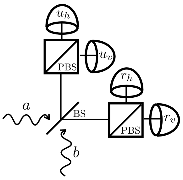
Figure S10: For a HOM–like experiment on two input photons $a$ and $b$, the setup involves one beam splitter (BS), two polarising beam splitters (PBS) and four non-photon-number-resolving photodetectors ($u_{h}$, $u_{v}$, $r_{h}$, and $r_{v}$).

We consider the setup presented in Fig. S10, with two photons combined on a 50:50 beam splitter. Each output path of the beam splitter contains a polarising beam splitter followed by two (non photon-number resolving) detectors. We are interested in two-click coincidence events on opposite outputs of the beam splitter, for the pairs $\{u_{h},r_{h}\},\{u_{v},r_{v}\},\{u_{v},r_{h}\},\{u_{h},r_{v}\}$. The rate of coincidence corresponding to a click at detector $u_{h}$ at time $t_{1}$ and a click at detector $r_{v}$ at time $t_{2}$ is labelled $\mathrm{det}_{h,v}(t_{1},t_{2})$, and similarly for the other pairs ($\mathrm{det}_{h,h}(t_{1},t_{2})$, $\mathrm{det}_{v,v}(t_{1},t_{2})$ and $\mathrm{det}_{v,h}(t_{1},t_{2})$). We define the probability to detect two clicks delayed by at most $T$ as

$$\mathrm{Det}_{h,v}(T):=\iint_{|t_{1}-t_{2}|\leq T}\mathrm{det}_{h,v}(t_{1},t_{2})\mathrm{d}t_{1}\mathrm{d}t_{2},$$ (180)

and similarly for the other coincidences.

I.2.2 Asymptotic visibilities

Mixed photon vs mixed photon

Assuming that all detectors have the same efficiency, the asymptotic visibility ($T\rightarrow+\infty$) of the HOM experiment is linked to the two-click coincidences:

$$V_{HOM}^{\infty} = 1-\frac{\mathrm{Det}_{h,h}(\infty)+\mathrm{Det}_{v,v}(\infty)}{\mathrm{Det}_{v,h}(\infty)+\mathrm{Det}_{h,v}(\infty)}$$ (183)

$$= 1-\frac{2\iint_{\mathbb{R}^{2}}\iint_{0}^{+\infty}\bar{P}_{a}(s_{a})\bar{P}_{b}(s_{b})\left|\Psi_{a}(t_{1}-s_{a})\Psi_{b}(t_{2}-s_{b})-\Psi_{a}(t_{2}-s_{a})\Psi_{b}(t_{1}-s_{b})\right|^{2}\mathrm{d}s_{a}\mathrm{d}s_{b}\mathrm{d}t_{1}\mathrm{d}t_{2}}{2\iint_{\mathbb{R}^{2}}\begin{array}[]{c}\left(\int_{0}^{+\infty}\bar{P}_{a}(s_{a})\left|\Psi_{a}(t_{2}-s_{a})\right|^{2}\mathrm{d}s_{a}\int_{0}^{+\infty}\bar{P}_{b}(s_{b})\left|\Psi_{b}(t_{1}-s_{b})\right|^{2}\mathrm{d}s_{b}\right.\\ \left.+\int_{0}^{+\infty}\bar{P}_{a}(s_{a})\left|\Psi_{a}(t_{1}-s_{a})\right|^{2}\mathrm{d}s_{a}\int_{0}^{+\infty}\bar{P}_{b}(s_{b})\left|\Psi_{b}(t_{2}-s_{b})\right|^{2}\mathrm{d}s_{b}\right)\end{array}\mathrm{d}t_{1}\mathrm{d}t_{2}}$$

$$= 1-\frac{2\iint_{0}^{+\infty}\bar{P}_{a}(s_{a})\bar{P}_{b}(s_{b})\iint_{\mathbb{R}^{2}}\left(\begin{array}[]{c}\left|\Psi_{a}(t_{1})\right|^{2}\left|\Psi_{b}(t_{2})\right|^{2}+\left|\Psi_{a}(t_{2})\right|^{2}\left|\Psi_{b}(t_{1})\right|^{2}\\ -2\mathrm{Re}\left(\Psi_{a}(t_{1}-s_{a})\Psi_{b}(t_{2}-s_{b})\Psi_{a}^{*}(t_{2}-s_{a})\Psi_{b}^{*}(t_{1}-s_{b})\right)\end{array}\right)\mathrm{d}t_{1}\mathrm{d}t_{2}\mathrm{d}s_{a}\mathrm{d}s_{b}}{4\iint_{0}^{+\infty}\bar{P}_{a}(s_{a})\bar{P}_{b}(s_{b})\mathrm{d}s_{a}\mathrm{d}s_{b}\int_{\mathbb{R}}\left|\Psi_{a}(t)\right|^{2}\mathrm{d}t\int_{\mathbb{R}}\left|\Psi_{b}(t)\right|^{2}\mathrm{d}t}$$

$$= 1-\frac{\int_{0}^{+\infty}\bar{P}_{a}(s_{a})\mathrm{d}s_{a}\int_{0}^{+\infty}\bar{P}_{b}(s_{b})\mathrm{d}s_{b}}{\iint_{0}^{+\infty}\bar{P}_{a}(s_{a})\bar{P}_{b}(s_{b})\mathrm{d}s_{a}\mathrm{d}s_{b}}+\frac{\iint_{0}^{+\infty}\bar{P}_{a}(s_{a})\bar{P}_{b}(s_{b})\left|\langle\Psi_{b}(\cdot-s_{b})|\Psi_{a}(\cdot-s_{a})\rangle\right|^{2}\mathrm{d}s_{a}\mathrm{d}s_{b}}{\iint_{0}^{+\infty}\bar{P}_{a}(s_{a})\bar{P}_{b}(s_{b})\mathrm{d}s_{a}\mathrm{d}s_{b}}$$

$$= \frac{1}{(1-P_{0,a})(1-P_{0,b})}\iint_{0}^{+\infty}\bar{P}_{a}(s_{a})\bar{P}_{b}(s_{b})\left|\langle\Psi_{b}(\cdot-s_{b})|\Psi_{a}(\cdot-s_{a})\rangle\right|^{2}\mathrm{d}s_{a}\mathrm{d}s_{b}$$

$$= \frac{1}{(1-P_{0,a})(1-P_{0,b})}\left(P_{ns,a}P_{ns,b}\left|\langle\Psi_{b}(\cdot)|\Psi_{a}(\cdot)\rangle\right|^{2}+P_{ns,a}\int_{0}^{+\infty}P_{b}(s_{b})\left|\langle\Psi_{b}(\cdot-s_{b})|\Psi_{a}(\cdot)\rangle\right|^{2}\mathrm{d}s_{b}\right.$$

$$\qquad\left.+P_{ns,b}\int_{0}^{+\infty}P_{a}(s_{a})\left|\langle\Psi_{b}(\cdot)|\Psi_{a}(\cdot-s_{a})\rangle\right|^{2}\mathrm{d}s_{a}+\iint_{0}^{+\infty}P_{a}(s_{a})P_{b}(s_{b})\left|\langle\Psi_{b}(\cdot-s_{b})|\Psi_{a}(\cdot-s_{a})\rangle\right|^{2}\mathrm{d}s_{a}\mathrm{d}s_{b}\right).$$

We have also assumed that for each emitter, the wavepackets for both polarisations are identical, and have used the fact that $\int_{\mathbb{R}}\left|\Psi_{a}(t)\right|^{2}\mathrm{d}t=1=\int_{\mathbb{R}}\left|\Psi_{b}(t)\right|^{2}\mathrm{d}t$.

If neither $a$ nor $b$ has a vacuum component, the visibility is

$$V_{HOM}^{\infty} = \iint_{0}^{+\infty}\bar{P}_{a}(s_{a})\bar{P}_{b}(s_{b})\left|\langle\Psi_{b}(\cdot-s_{b})|\Psi_{a}(\cdot-s_{a})\rangle\right|^{2}\mathrm{d}s_{a}\mathrm{d}s_{b}.$$ (188)

Pure photon vs mixed photon

In the case where photon $a$ is mixed and photon $b$ is either pure or lost, we take $P_{ns,b}=1-P_{0,b}$ and $\forall s\quad P_{b}(s)=0$, so that

$$V_{HOM}^{\infty,pure-mixed} = \frac{1}{1-P_{0,a}}\int_{0}^{+\infty}\bar{P}_{a}(s_{a})\left|\langle\Psi_{b}(\cdot)|\Psi_{a}(\cdot-s_{a})\rangle\right|^{2}\mathrm{d}s_{a},$$ (189)

which is the fidelity between the two photon states.

Pure photon vs pure photon

In the case where both photons $a$ and $b$ are pure without any vacuum component, we take $P_{0,a}=P_{0,b}=0$, $\forall s\quad P_{a}(s)=0=P_{b}(s)$ and $P_{ns,a}=P_{ns,b}=1$ so that

$$V_{HOM}^{\infty,pure-pure}=\left|\langle\Psi_{b}(\cdot)|\Psi_{a}(\cdot)\rangle\right|^{2},$$ (190)

which is again nothing more than the overlap between the two photon states, or their fidelity.

I.2.3 Visibilities

Above, we considered all possible coincidences, with a window length $T\rightarrow+\infty$. Instead, one could look at finite $T$ and compute the integrals for $t_{1},t_{2}$ such that $\left|t_{1}-t_{2}\right|\leq T$ (rather than over $\mathds{R}^{2}$). This computation is more involved and typically requires numerical methods to estimate the integrals (see Appendix H). It is observed that the visibility decreases with $T$ [24] and goes to $1$ in the pure-vs-pure case when $T\rightarrow 0$.

References

- Simon [2017] C. Simon, Towards a global quantum network, Nature Photonics 11, 678 (2017).
- Friis et al. [2018] N. Friis, O. Marty, C. Maier, C. Hempel, M. Holzäpfel, P. Jurcevic, M. B. Plenio, M. Huber, C. Roos, R. Blatt, and B. Lanyon, Observation of Entangled States of a Fully Controlled 20-Qubit System, Physical Review X 8, 021012 (2018).
- Moses et al. [2023] S. A. Moses, C. H. Baldwin, M. S. Allman, R. Ancona, L. Ascarrunz, C. Barnes, J. Bartolotta, B. Bjork, P. Blanchard, M. Bohn, J. G. Bohnet, N. C. Brown, N. Q. Burdick, W. C. Burton, S. L. Campbell, J. P. Campora, C. Carron, J. Chambers, J. W. Chan, Y. H. Chen, A. Chernoguzov, E. Chertkov, J. Colina, J. P. Curtis, R. Daniel, M. DeCross, D. Deen, C. Delaney, J. M. Dreiling, C. T. Ertsgaard, J. Esposito, B. Estey, M. Fabrikant, C. Figgatt, C. Foltz, M. Foss-Feig, D. Francois, J. P. Gaebler, T. M. Gatterman, C. N. Gilbreth, J. Giles, E. Glynn, A. Hall, A. M. Hankin, A. Hansen, D. Hayes, B. Higashi, I. M. Hoffman, B. Horning, J. J. Hout, R. Jacobs, J. Johansen, L. Jones, J. Karcz, T. Klein, P. Lauria, P. Lee, D. Liefer, S. T. Lu, D. Lucchetti, C. Lytle, A. Malm, M. Matheny, B. Mathewson, K. Mayer, D. B. Miller, M. Mills, B. Neyenhuis, L. Nugent, S. Olson, J. Parks, G. N. Price, Z. Price, M. Pugh, A. Ransford, A. P. Reed, C. Roman, M. Rowe, C. Ryan-Anderson, S. Sanders, J. Sedlacek, P. Shevchuk, P. Siegfried, T. Skripka, B. Spaun, R. T. Sprenkle, R. P. Stutz, M. Swallows, R. I. Tobey, A. Tran, T. Tran, E. Vogt, C. Volin, J. Walker, A. M. Zolot, and J. M. Pino, A Race-Track Trapped-Ion Quantum Processor, Physical Review X 13, 041052 (2023).
- Wang et al. [2021] P. Wang, C.-Y. Luan, M. Qiao, M. Um, J. Zhang, Y. Wang, X. Yuan, M. Gu, J. Zhang, and K. Kim, Single ion qubit with estimated coherence time exceeding one hour, Nature Communications 12, 233 (2021).
- Bock et al. [2018] M. Bock, P. Eich, S. Kucera, M. Kreis, A. Lenhard, C. Becher, and J. Eschner, High-fidelity entanglement between a trapped ion and a telecom photon via quantum frequency conversion, Nature Communications 9, 1998 (2018).
- Duan and Monroe [2010] L.-M. Duan and C. Monroe, Colloquium : Quantum networks with trapped ions, Reviews of Modern Physics 82, 1209 (2010).
- Bruzewicz et al. [2019] C. D. Bruzewicz, J. Chiaverini, R. McConnell, and J. M. Sage, Trapped-ion quantum computing: Progress and challenges, Applied Physics Reviews 6, 021314 (2019).
- Zhong et al. [2015] M. Zhong, M. P. Hedges, R. L. Ahlefeldt, J. G. Bartholomew, S. E. Beavan, S. M. Wittig, J. J. Longdell, and M. J. Sellars, Optically addressable nuclear spins in a solid with a six-hour coherence time, Nature 517, 177 (2015).
- Clausen et al. [2011] C. Clausen, I. Usmani, F. Bussières, N. Sangouard, M. Afzelius, H. De Riedmatten, and N. Gisin, Quantum storage of photonic entanglement in a crystal, Nature 469, 508 (2011).
- Saglamyurek et al. [2011] E. Saglamyurek, N. Sinclair, J. Jin, J. A. Slater, D. Oblak, F. Bussières, M. George, R. Ricken, W. Sohler, and W. Tittel, Broadband waveguide quantum memory for entangled photons, Nature 469, 512 (2011).
- Businger et al. [2022] M. Businger, L. Nicolas, T. S. Mejia, A. Ferrier, P. Goldner, and M. Afzelius, Non-classical correlations over 1250 modes between telecom photons and 979-nm photons stored in 171Yb3+:Y2SiO5, Nature Communications 13, 6438 (2022).
- Sinclair et al. [2014] N. Sinclair, E. Saglamyurek, H. Mallahzadeh, J. A. Slater, M. George, R. Ricken, M. P. Hedges, D. Oblak, C. Simon, W. Sohler, and W. Tittel, Spectral Multiplexing for Scalable Quantum Photonics using an Atomic Frequency Comb Quantum Memory and Feed-Forward Control, Physical Review Letters 113, 053603 (2014).
- Sangouard et al. [2011] N. Sangouard, C. Simon, H. de Riedmatten, and N. Gisin, Quantum repeaters based on atomic ensembles and linear optics, Reviews of Modern Physics 83, 33 (2011).
- Farrera et al. [2016] P. Farrera, G. Heinze, B. Albrecht, M. Ho, M. Chávez, C. Teo, N. Sangouard, and H. De Riedmatten, Generation of single photons with highly tunable wave shape from a cold atomic ensemble, Nature Communications 7, 13556 (2016).
- Morin et al. [2019] O. Morin, M. Körber, S. Langenfeld, and G. Rempe, Deterministic Shaping and Reshaping of Single-Photon Temporal Wave Functions, Physical Review Letters 123, 133602 (2019).
- Moehring et al. [2007] D. L. Moehring, P. Maunz, S. Olmschenk, K. C. Younge, D. N. Matsukevich, L.-M. Duan, and C. Monroe, Entanglement of single-atom quantum bits at a distance, Nature 449, 68 (2007).
- Stephenson et al. [2020] L. J. Stephenson, D. P. Nadlinger, B. C. Nichol, S. An, P. Drmota, T. G. Ballance, K. Thirumalai, J. F. Goodwin, D. M. Lucas, and C. J. Ballance, High-Rate, High-Fidelity Entanglement of Qubits Across an Elementary Quantum Network, Physical Review Letters 124, 110501 (2020).
- Krutyanskiy et al. [2023a] V. Krutyanskiy, M. Galli, V. Krcmarsky, S. Baier, D. A. Fioretto, Y. Pu, A. Mazloom, P. Sekatski, M. Canteri, M. Teller, J. Schupp, J. Bate, M. Meraner, N. Sangouard, B. P. Lanyon, and T. E. Northup, Entanglement of Trapped-Ion Qubits Separated by 230 Meters, Physical Review Letters 130, 050803 (2023a).
- Saha et al. [2024] S. Saha, M. Shalaev, J. O’Reilly, I. Goetting, G. Toh, A. Kalakuntla, Y. Yu, and C. Monroe, High-fidelity remote entanglement of trapped atoms mediated by time-bin photons (2024), arXiv:2406.01761 [quant-ph] .
- Krutyanskiy et al. [2019] V. Krutyanskiy, M. Meraner, J. Schupp, V. Krcmarsky, H. Hainzer, and B. P. Lanyon, Light-matter entanglement over 50 km of optical fibre, npj Quantum Information 5, 72 (2019).
- Lago-Rivera et al. [2021] D. Lago-Rivera, S. Grandi, J. V. Rakonjac, A. Seri, and H. De Riedmatten, Telecom-heralded entanglement between multimode solid-state quantum memories, Nature 594, 37 (2021).
- Liu et al. [2021] X. Liu, J. Hu, Z.-F. Li, X. Li, P.-Y. Li, P.-J. Liang, Z.-Q. Zhou, C.-F. Li, and G.-C. Guo, Heralded entanglement distribution between two absorptive quantum memories, Nature 594, 41 (2021).
- Duan et al. [2001] L.-M. Duan, M. D. Lukin, J. I. Cirac, and P. Zoller, Long-distance quantum communication with atomic ensembles and linear optics, Nature 414, 413 (2001).
- Meraner et al. [2020] M. Meraner, A. Mazloom, V. Krutyanskiy, V. Krcmarsky, J. Schupp, D. A. Fioretto, P. Sekatski, T. E. Northup, N. Sangouard, and B. P. Lanyon, Indistinguishable photons from a trapped-ion quantum network node, Physical Review A 102, 052614 (2020).
- De Riedmatten et al. [2008] H. De Riedmatten, M. Afzelius, M. U. Staudt, C. Simon, and N. Gisin, A solid-state light–matter interface at the single-photon level, Nature 456, 773 (2008).
- Gündoğan et al. [2015] M. Gündoğan, P. M. Ledingham, K. Kutluer, M. Mazzera, and H. De Riedmatten, Solid State Spin-Wave Quantum Memory for Time-Bin Qubits, Physical Review Letters 114, 230501 (2015).
- Laplane et al. [2016] C. Laplane, P. Jobez, J. Etesse, N. Timoney, N. Gisin, and M. Afzelius, Multiplexed on-demand storage of polarization qubits in a crystal, New Journal of Physics 18, 013006 (2016).
- Rakonjac et al. [2021] J. V. Rakonjac, D. Lago-Rivera, A. Seri, M. Mazzera, S. Grandi, and H. De Riedmatten, Entanglement between a Telecom Photon and an On-Demand Multimode Solid-State Quantum Memory, Physical Review Letters 127, 210502 (2021).
- Seri et al. [2017] A. Seri, A. Lenhard, D. Rieländer, M. Gündoğan, P. M. Ledingham, M. Mazzera, and H. De Riedmatten, Quantum Correlations between Single Telecom Photons and a Multimode On-Demand Solid-State Quantum Memory, Physical Review X 7, 021028 (2017).
- Afzelius et al. [2009] M. Afzelius, C. Simon, H. de Riedmatten, and N. Gisin, Multimode quantum memory based on atomic frequency combs, Physical Review A 79, 052329 (2009).
- Afzelius and Simon [2010] M. Afzelius and C. Simon, Impedance-matched cavity quantum memory, Physical Review A 82, 022310 (2010).
- Moiseev et al. [2010] S. A. Moiseev, S. N. Andrianov, and F. F. Gubaidullin, Efficient multimode quantum memory based on photon echo in an optimal QED cavity, Physical Review A 82, 022311 (2010).
- Afzelius et al. [2013] M. Afzelius, N. Sangouard, G. Johansson, M. U. Staudt, and C. M. Wilson, Proposal for a coherent quantum memory for propagating microwave photons, New Journal of Physics 15, 065008 (2013).
- Hong et al. [1987] C. K. Hong, Z. Y. Ou, and L. Mandel, Measurement of subpicosecond time intervals between two photons by interference, Physical Review Letters 59, 2044 (1987).
- Duranti et al. [2024] S. Duranti, S. Wengerowsky, L. Feldmann, A. Seri, B. Casabone, and H. De Riedmatten, Efficient cavity-assisted storage of photonic qubits in a solid-state quantum memory, Optics Express 32, 26884 (2024).
- Collett and Gardiner [1984] M. J. Collett and C. W. Gardiner, Squeezing of intracavity and traveling-wave light fields produced in parametric amplification, Physical Review A 30, 1386 (1984).
- Gardiner and Collett [1985] C. W. Gardiner and M. J. Collett, Input and output in damped quantum systems: Quantum stochastic differential equations and the master equation, Physical Review A 31, 3761 (1985).
- Gardiner and Zoller [2004] C. W. Gardiner and P. Zoller, Quantum Noise: A Handbook of Markovian and Non-Markovian Quantum Stochastic Methods with Applications to Quantum Optics, 3rd ed., Springer Series in Synergetics (Springer, Berlin ; New York, 2004).
- Gorshkov et al. [2007a] A. V. Gorshkov, A. André, M. D. Lukin, and A. S. Sørensen, Photon storage in -type optically dense atomic media. I. Cavity model, Physical Review A 76, 033804 (2007a).
- Gorshkov et al. [2007b] A. V. Gorshkov, A. André, M. D. Lukin, and A. S. Sørensen, Photon storage in -type optically dense atomic media. III. Effects of inhomogeneous broadening, Physical Review A 76, 033806 (2007b).
- Simon et al. [2007] C. Simon, H. De Riedmatten, M. Afzelius, N. Sangouard, H. Zbinden, and N. Gisin, Quantum Repeaters with Photon Pair Sources and Multimode Memories, Physical Review Letters 98, 190503 (2007).
- Keller et al. [2004] M. Keller, B. Lange, K. Hayasaka, W. Lange, and H. Walther, Continuous generation of single photons with controlled waveform in an ion-trap cavity system, Nature 431, 1075 (2004).
- Schupp et al. [2021] J. Schupp, V. Krcmarsky, V. Krutyanskiy, M. Meraner, T. Northup, and B. Lanyon, Interface between Trapped-Ion Qubits and Traveling Photons with Close-to-Optimal Efficiency, PRX Quantum 2, 020331 (2021).
- Fabre and Treps [2020] C. Fabre and N. Treps, Modes and states in quantum optics, Reviews of Modern Physics 92, 035005 (2020).
- Legero et al. [2006] T. Legero, T. Wilk, A. Kuhn, and G. Rempe, Characterization of Single Photons Using Two-Photon Interference, in Advances In Atomic, Molecular, and Optical Physics, Vol. 53 (Elsevier, 2006) pp. 253–289.
- Craddock et al. [2019] A. N. Craddock, J. Hannegan, D. P. Ornelas-Huerta, J. D. Siverns, A. J. Hachtel, E. A. Goldschmidt, J. V. Porto, Q. Quraishi, and S. L. Rolston, Quantum Interference between Photons from an Atomic Ensemble and a Remote Atomic Ion, Physical Review Letters 123, 213601 (2019).
- Krutyanskiy et al. [2023b] V. Krutyanskiy, M. Canteri, M. Meraner, J. Bate, V. Krcmarsky, J. Schupp, N. Sangouard, and B. P. Lanyon, Telecom-Wavelength Quantum Repeater Node Based on a Trapped-Ion Processor, Physical Review Letters 130, 213601 (2023b).
- Van Leent et al. [2020] T. Van Leent, M. Bock, R. Garthoff, K. Redeker, W. Zhang, T. Bauer, W. Rosenfeld, C. Becher, and H. Weinfurter, Long-Distance Distribution of Atom-Photon Entanglement at Telecom Wavelength, Physical Review Letters 124, 010510 (2020).
- Geus et al. [2024] J. F. Geus, F. Elsen, S. Nyga, A. J. Stolk, K. L. Van Der Enden, E. J. Van Zwet, C. Haefner, R. Hanson, and B. Jungbluth, Low-noise short-wavelength pumped frequency downconversion for quantum frequency converters, Optica Quantum 2, 189 (2024).
- Krutyanskiy et al. [2024] V. Krutyanskiy, M. Canteri, M. Meraner, V. Krcmarsky, and B. Lanyon, Multimode Ion-Photon Entanglement over 101 Kilometers, PRX Quantum 5, 020308 (2024).
- Gorshkov et al. [2007c] A. V. Gorshkov, A. André, M. D. Lukin, and A. S. Sørensen, Photon storage in -type optically dense atomic media. II. Free-space model, Physical Review A 76, 033805 (2007c).
- [52] D. A. Steck, Quantum and Atom Optics.
- Kollath-Bönig et al. [2024] J. S. Kollath-Bönig, L. Dellantonio, L. Giannelli, T. Schmit, G. Morigi, and A. S. Sørensen, Fast storage of photons in cavity-assisted quantum memories, Physical Review Applied 22, 044038 (2024).
- Hird [2021] T. M. Hird, Engineering a Noise-Free Quantum Memory for Temporal Mode Manipulation, Ph.D. thesis, Oxford (2021).
- Lax [1966] M. Lax, Quantum Noise. IV. Quantum Theory of Noise Sources, Physical Review 145, 110 (1966).
- Caves [1982] C. M. Caves, Quantum limits on noise in linear amplifiers, Physical Review D 26, 1817 (1982).
- Yurke and Denker [1984] B. Yurke and J. S. Denker, Quantum network theory, Physical Review A 29, 1419 (1984).
- Macfarlane and Shelby [1987] R. Macfarlane and R. Shelby, Coherent Transient and Holeburning Spectroscopy of Rare Earth Ions in Solids, in Modern Problems in Condensed Matter Sciences, Vol. 21 (Elsevier, 1987) pp. 51–184.
- Maniloff et al. [1995] E. S. Maniloff, F. R. Graf, H. Gygax, S. B. Altner, S. Bernet, A. Renn, and U. P. Wild, Power broadening of the spectral hole width in an optically thick sample, Chemical Physics 193, 173 (1995).
- Nilsson et al. [2004] M. Nilsson, L. Rippe, S. Kröll, R. Klieber, and D. Suter, Hole-burning techniques for isolation and study of individual hyperfine transitions in inhomogeneously broadened solids demonstrated in Pr 3 + : Y 2 SiO 5, Physical Review B 70, 214116 (2004).
- Lukin and Childress [2016] M. D. Lukin and L. Childress, Modern Atomic and Optical Physics II (Decembre 2016).
- Sangouard et al. [2007] N. Sangouard, C. Simon, M. Afzelius, and N. Gisin, Analysis of a quantum memory for photons based on controlled reversible inhomogeneous broadening, Physical Review A 75, 032327 (2007).
- Chanelière et al. [2018] T. Chanelière, G. Hétet, and N. Sangouard, Quantum Optical Memory Protocols in Atomic Ensembles, in Advances In Atomic, Molecular, and Optical Physics, Vol. 67 (Elsevier, 2018) pp. 77–150.
- Lugiato et al. [1984] L. A. Lugiato, P. Mandel, and L. M. Narducci, Adiabatic elimination in nonlinear dynamical systems, Physical Review A 29, 1438 (1984).
- Dicke [1954] R. H. Dicke, Coherence in Spontaneous Radiation Processes, Physical Review 93, 99 (1954).
- Gardiner and Zoller [2015] C. W. Gardiner and P. Zoller, The Quantum World of Ultra-Cold Atoms and Light Book II The Physics of Quantum-Optical Devices, Cold Atoms No. 4 (Imperial College Press, London, 2015).
- Dubetskiĭ and Chebotaev [1985] B. Ya. Dubetskiĭ and V. P. Chebotaev, Echos in classical and quantum ensembles with determinate frequencies, JETP Lett. Pis’ma Zh. Eksp. Teor. Fiz., 41, 267 (1985).
- Jobez et al. [2016] P. Jobez, N. Timoney, C. Laplane, J. Etesse, A. Ferrier, P. Goldner, N. Gisin, and M. Afzelius, Towards highly multimode optical quantum memory for quantum repeaters, Physical Review A 93, 032327 (2016).
- Bonarota et al. [2010] M. Bonarota, J. Ruggiero, J. L. L. Gouët, and T. Chanelière, Efficiency optimization for atomic frequency comb storage, Physical Review A 81, 033803 (2010).
- Zang et al. [2024] A. Zang, M. Suchara, and T. Zhong, Provable Optimality of the Square-Tooth Atomic Frequency Comb Quantum Memory (2024), arXiv:2406.01769 [quant-ph] .
- Bonarota et al. [2012] M. Bonarota, J.-L. Le Gouët, S. A. Moiseev, and T. Chanelière, Atomic frequency comb storage as a slow-light effect, Journal of Physics B: Atomic, Molecular and Optical Physics 45, 124002 (2012).
- Souza et al. [2012] A. M. Souza, G. A. Álvarez, and D. Suter, Robust dynamical decoupling, Philosophical Transactions of the Royal Society A: Mathematical, Physical and Engineering Sciences 370, 4748 (2012).
- Duranti [2023] S. Duranti, Towards Efficient Quantum Repeater Nodes Based on Solid-State Quantum Memories, Ph.D. thesis, Universitat Politècnica de Catalunya (2023).
- Shore [2011] B. W. Shore, Manipulating Quantum Structures Using Laser Pulses (Cambridge University Press, Cambridge, UK ; New York, 2011).
- Ortu et al. [2022] A. Ortu, J. V. Rakonjac, A. Holzäpfel, A. Seri, S. Grandi, M. Mazzera, H. De Riedmatten, and M. Afzelius, Multimode capacity of atomic-frequency comb quantum memories, Quantum Science and Technology 7, 035024 (2022).
- Scully and Zubairy [1997] M. O. Scully and M. S. Zubairy, Quantum Optics (Cambridge University Press, Cambridge ; New York, 1997).
- Cohen-Tannoudji et al. [2001] C. Cohen-Tannoudji, J. Dupont-Roc, and G. Grynberg, Processus d’interaction entre photons et atomes, Savoirs actuels Physique (EDP Sciences [u.a.], Les Ulis, 2001).
- Carmichael [1999] H. Carmichael, Statistical Methods in Quantum Optics 1 : Master Equations and Fokker-Planck Equations, Texts and Monographs in Physics (Springer, New York, 1999).
- Hald and Polzik [2001] J. Hald and E. S. Polzik, Mapping a quantum state of light onto atoms, Journal of Optics B: Quantum and Semiclassical Optics 3, S83 (2001).
- Kurucz et al. [2011] Z. Kurucz, J. H. Wesenberg, and K. Mølmer, Spectroscopic properties of inhomogeneously broadened spin ensembles in a cavity, Physical Review A 83, 053852 (2011).
- Mollow [1975] B. R. Mollow, Pure-state analysis of resonant light scattering: Radiative damping, saturation, and multiphoton effects, Physical Review A 12, 1919 (1975).
- Blow et al. [1990] K. J. Blow, R. Loudon, S. J. D. Phoenix, and T. J. Shepherd, Continuum fields in quantum optics, Physical Review A 42, 4102 (1990).
- Moiseev et al. [2024] S. A. Moiseev, K. I. Gerasimov, M. M. Minnegaliev, and E. S. Moiseev, Optical quantum memory on macroscopic coherence (2024), arXiv:2408.09991 [physics, physics:quant-ph] .
- Fejér [1910] L. Fejér, Lebesguessche Konstanten und divergente Fourierreihen, Journal für die reine und angewandte Mathematik 138, 22 (1910).
- Young [1988] N. Young, An Introduction to Hilbert Space, 1st ed. (Cambridge University Press, 1988).
- Motzoi and Mølmer [2018] F. Motzoi and K. Mølmer, Precise single-qubit control of the reflection phase of a photon mediated by a strongly-coupled ancilla–cavity system, New Journal of Physics 20, 053029 (2018).
- Kiilerich and Mølmer [2019] A. H. Kiilerich and K. Mølmer, Input-Output Theory with Quantum Pulses, Physical Review Letters 123, 123604 (2019).
- Bernád et al. [2024] J. Z. Bernád, M. Schilling, Y. Wen, M. M. Müller, T. Calarco, P. Bertet, and F. Motzoi, Analytical solutions for optimal photon absorption into inhomogeneous spin memories (2024), arXiv:2401.04717 [quant-ph] .
- Lehmann et al. [1955] H. Lehmann, K. Symanzik, and W. Zimmermann, Zur Formulierung quantisierter Feldtheorien, Il Nuovo Cimento 1, 205 (1955).
- Fan et al. [2010] S. Fan, Ş. E. Kocaba\textcommabelows, and J.-T. Shen, Input-output formalism for few-photon transport in one-dimensional nanophotonic waveguides coupled to a qubit, Physical Review A 82, 063821 (2010).
- Raimond [2013] J.-M. Raimond, Atoms and Photons, université pierre et marie curie, département de physique de l’ecole normal supérieure ed. (Laboratoire Kastler Brossel, 2013).
- Siegman [1986] A. E. Siegman, Lasers (University Science Books, Mill Valley, California, 1986).
- Sekatski et al. [2011] P. Sekatski, N. Sangouard, N. Gisin, H. De Riedmatten, and M. Afzelius, Photon-pair source with controllable delay based on shaped inhomogeneous broadening of rare-earth-metal-doped solids, Physical Review A 83, 053840 (2011).
- Crisp [1970] M. D. Crisp, Propagation of Small-Area Pulses of Coherent Light through a Resonant Medium, Physical Review A 1, 1604 (1970).
- Chanelière et al. [2010] T. Chanelière, J. Ruggiero, M. Bonarota, M. Afzelius, and J.-L. Le Gouët, Efficient light storage in a crystal using an atomic frequency comb, New Journal of Physics 12, 023025 (2010).
- Afzelius et al. [2010] M. Afzelius, I. Usmani, A. Amari, B. Lauritzen, A. Walther, C. Simon, N. Sangouard, J. Minář, H. De Riedmatten, N. Gisin, and S. Kröll, Demonstration of Atomic Frequency Comb Memory for Light with Spin-Wave Storage, Physical Review Letters 104, 040503 (2010).