The outflow impacts on the size of the narrow-line region among type-2 AGNs

Abstract

We present the study of the gas kinematics in narrow-line regions (NLRs) of $2{,}009$ type-2 AGNs at $z<0.34$. We construct the [O III] $\lambda$5007  emission-line images using publicly available broadband images from the Sloan Digital Sky Survey (SDSS). The [O III] emission area of the samples, measured down to $1.7\times 10^{-15}$ erg s^-1 cm^-2 arcsec^-2, ranges from $3.7$ kpc² up to $224$ kpc². With our broadband technique, we found the strong correlation between [O III] area and AGN luminosity inferred from the [O III] luminosity and the mid-infrared luminosity at the rest-frame $15\mu$m. The isophotal threshold used to determine the [O III] area affects the correlation strength in that the brighter isophote yields the stronger correlation between the [O III] area and AGN luminosity. The presence of gas outflow is examined by the ratio of the [O III] velocity dispersion to the stellar velocity dispersion ($\sigma_{\rm[O\,III]}/\sigma_{\star}>1.4$) using the SDSS spectra. At the given luminosity, the objects with and without outflows exhibit the same extension of the [O III] emission. Their correlation between the [O III] area and luminosity is almost identical. It is suggested that the size of NLRs is not affected by outflow mechanisms but rather by photoionization from the central AGNS.

tablenum SIXtablenum

1 INTRODUCTION

Observational evidence on the co-evolution between galaxy properties and the growth of supermassive black holes (SMBHs) at the galactic center has increased significantly over the past few decades (e.g., Silk & Rees, 1998; Gültekin et al., 2009; Kormendy & Ho, 2013; Baldassare et al., 2020). The evolution of the BH accretion rate and the star formation rate density are coincidentally found to be similar; they reach a peak at $z\sim 2$ and decrease until the present epoch (e.g., Madau et al., 1996; Hopkins et al., 2007; Aird et al., 2015; Carraro et al., 2020), supporting the idea that the evolution of SMBHs and galaxies is closely connected (Lynden-Bell, 1969; Osterbrock & Ferland, 2006).

The hydrodynamic simulations by Hopkins & Quataert (2010) show that BH accretion and the star formation rate (SFR) depend on the availability of the cold gas. When the gas is used up, the star formation terminates and the luminosity of the active galactic nucleus (AGN) fades rapidly, marking the galaxy as the red elliptical galaxy with little-to-no SFR or BH accretion (Lapi et al., 2006). This coupling has been proposed to explain the observed correlation between the mass of SMBH and the bulge stellar mass (Magorrian et al., 1998; Scott et al., 2013), or the bulge stellar velocity dispersion (Kormendy & Ho, 2013; Saglia et al., 2016).

It is believed that the energy released from AGN might play a crucial role in regulating the gas cycle in the host galaxy known as AGN feedback (Croton et al., 2006; Somerville et al., 2008; Fabian, 2012). Current cosmological models of galaxy evolution (e.g., Bower et al., 2006; Croton et al., 2006; Somerville & Davé, 2015; Pillepich et al., 2019) require AGN feedback to suppress star formation in massive galaxies to reproduce the observed galaxy luminosity function at the high-luminosity end. The energy emitted from the central AGNs disturbs the cold gas reservoir by either heating (radiative feedback) or expelling them as outflows (mechanical feedback). The gas outflows have been detected by numerous studies (e.g., Woo et al., 2016; Torres-Papaqui et al., 2020), however, their impact on the global SFR of the host galaxy evolution is still unclear. Some studies have found that outflows can deplete the cold gas in the interstellar medium (ISM), which is used to form new stars (Wylezalek & Zakamska, 2016; Chen et al., 2022), terminating the star formation. Conversely, outflows are found to enhance the SFR by triggering the formation of new stars within outflows themselves, or by feeding the gas back to the interstellar medium (Shin et al., 2019; Zhuang & Ho, 2020; Riffel et al., 2024). Verifying the outflow impacts on the AGN and host galaxies is difficult as it requires knowledge of various parameters such as spatial extent of an outflow, outflow velocity, mass loss rate, etc.

One approach to study gas outflows driven by AGNs is to investigate the most extensive part of the AGNs called the narrow-line region (NLR). It has a size of $0.1-10$ kpc extended from the nucleus, which is spatially resolved in nearby galaxies. The NLR consists of gas clouds ionized by the central AGN, exhibiting multiple emission lines (e.g., [O III] $\lambda\lambda$4959,5007, [S II]$\lambda\lambda 6716,6731$, [O II]$\lambda\lambda 3729,3726$). The size of the NLR is usually measured by the [O III] $\lambda$5007 emission lines (hereafter, [O III]), as it is one of the most prominent emission lines. The [O III] line has also been extensively used to study the warm ionised outflows (Woo et al., 2016; Kang & Woo, 2018). Hence, using this emission line could give us insight into both the spatial extent and also the outflow kinematics in the NLR.

Cardamone et al. (2009) identified galaxies with extremely strong [O III] $\lambda\lambda$4959,5007 emission lines using the magnitude difference between two broadband images with and without contributions of the emission line. This technique has been used over the past decade by several studies (e.g., Izotov et al., 2011; Liu et al., 2022). Using similar technique but with the narrowband images, various studies were able to classify galaxies with spatially extended emission lines and related them to outflow mechanisms (e.g., Yuma et al., 2013; Harikane et al., 2014; Yuma et al., 2017, 2019). Recently, Sun et al. (2018) used the broadband images from the Subaru Hyper Suprime-Cam (HSC) survey to detect the resolved [O III] emission in a sample of $300$ type-2 AGNs. They have found a strong correlation between the [O III] area and AGN luminosity. However, the correlation of [O III] emission with gas kinematics or outflows has not been yet explored.

In this work, we aim to investigate the impact of outflows on the size of NLR. We constructed the [O III] images using the broadband images and spectra from the Sloan Digital Sky Surveys (SDSS, York et al., 2000). The gaseous kinematics and outflows are determined from the [O III] emission line taken from the SDSS spectroscopic data in the integrated $3\text{\,}\mathrm{\SIUnitSymbolArcsecond}$ fiber. The paper is organized as follows. Section 2 provides information on our samples and data. The construction of [O III] images and the area measurement are explained in Section 3. We described the [O III] kinematics and outflow selection in Section 4. Our results are shown in Section 5. We discuss the results of the size-luminosity relations and the outflow impacts in Section 6 and summarize in Section 7. Throughout this work, we assumed a flat $\Lambda$CDM cosmology with an $h=0.7$, $\Omega_{m}=0.3$, $\Omega_{\Lambda}=0.7$.

2 SAMPLE AND DATA

2.1 Sample Selection

A sample of type-2 AGNs at $0.13<z<0.34$ was selected from an object classified as “Seyfert” in the SDSS “emissionlinesport” table reported by Thomas et al. (2013). The “Seyfert” label in the catalog was classified based on the [N II]-based BPT diagnostic diagrams (Baldwin et al., 1981; Kewley et al., 2001; Schawinski et al., 2007). That is the diagram between the emission-line ratios of [O III] $\lambda 5007$/H$\beta$ and those of [N II] $\lambda 6583$/H$\alpha$. The redshift ranges are calculated such that the [O III] $\lambda\lambda$4959,5007 emission lines fall within the full width at half maximum (FWHM) of the SDSS-$r$ filter. We finally obtained a sample of $2{,}724$ type-2 AGNs with the [O III] luminosity in the range of $\log(L_{\mathrm{[O\;III]}}/\mathrm{erg\,s^{-1}})=40.0-43.0$. Figure 1 shows the redshifts and [O III] emission line luminosity of all samples. The [O III] luminosity distributes equally over the redshift.

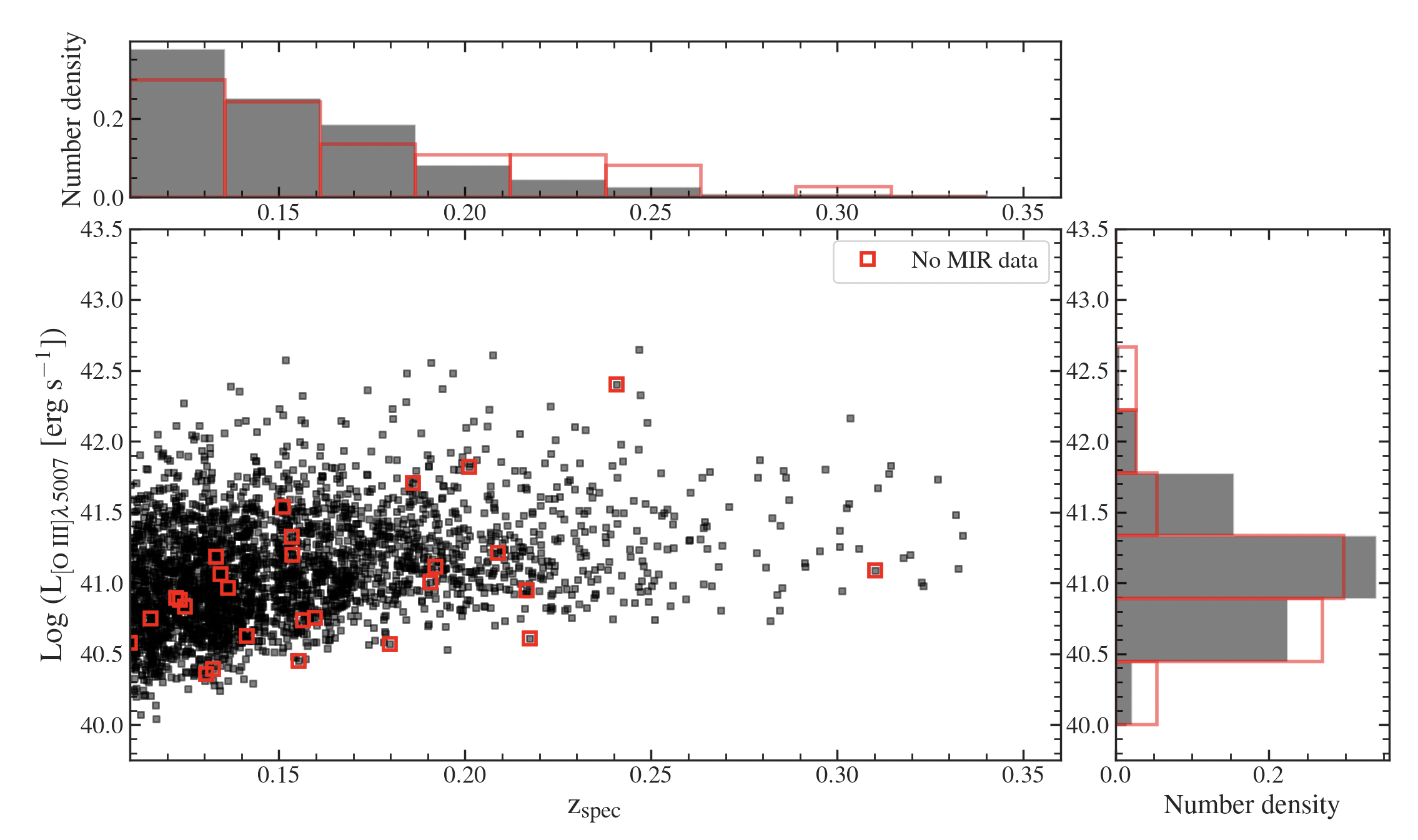
Figure 1: L${}_{\mathrm{[O\;III]\lambda 5007}}$ vs spectroscopic redshift ($z_{\mathrm{spec}}$) of $2{,}724$ type-2 AGNs at $0.13<z<0.34$. The solid black and open red squares represent the samples with and without WISE/MIR detection, respectively (see Section 2.3). The histograms in the x-axis and y-axis show the distribution of $z_{\mathrm{spec}}$ and L${}_{\mathrm{[O\;III]\lambda 5007}}$ for samples with MIR detections (black) and no MIR detections (red), respectively.

2.2 SDSS Images and Spectra

The broadband images and spectra are retrieved from SDSS Data Release 12 (Alam et al., 2015). We used broadband $r,i$ and $z$ images covering the wavelength range of $5{,}400$Å $-11{,}000$Å with the median $5\sigma$ limiting magnitude for point sources of $22.70,22.20$, and $20.71$ mag, respectively. All the images are registered to the World Coordinate System (WCS) with a pixel scale of $0.396\text{\,}\arcsec$, which corresponds to $0.8-1.9$ kpc at the redshift range of our sample. For each object, we crop the image to the size of $40\text{\,}\arcsec$$\times$$40\text{\,}\arcsec$ centering at the target in the $r$-band image.

The spectral data are taken with the SDSS spectrograph with a fiber diameter of $3\text{\,}\arcsec$ corresponding to a physical diameter of $6.0$–$14.5$ kpc. The wavelength coverage is $3{,}800$–$9{,}200$ Å with a resolution of $R\sim 1{,}500$ at $3{,}800$ Å, and $R\sim 2{,}500$ at $9{,}000$ Å.

2.3 Mid-infrared data from WISE

The mid-infrared (MIR) data are obtained from the Wide-field Infrared Survey Explorer (WISE; Wright et al., 2010). The all-sky survey has been conducted in four bands: W1 (3.4$\mu$m), W2 (4.6$\mu$m), W3 (12$\mu$m), and W4 (22$\mu$m). The positions and photometry of WISE/MIR objects are described in the WISE ALL-SKY release source catalog. We cross-matched our AGN sample with the WISE/MIR objects within a radius of $1\arcsec$. We adopted the same matching radius as used by Greenwell et al. (2023), which covers $86.4\%$ of the closest SDSS-WISE associates. Eventually, we obtained $3{,}692$ ($\sim 97\%$) MIR counterparts, while $130$ type-2 AGNs in our sample had no match in the WISE catalog (open red squares in Figure 1).

We estimate the bolometric luminosity by using the mid-infrared luminosity to instead of generally used $L_{\mathrm{[OIII]}}$ (Heckman et al., 2004), as the $\mathrm{[OIII]}$ emission can be affected by dust extinction within the NLRs. The MIR emission is less sensitive to dust absorption than the optical emission lines. The detailed calculation of the bolometric luminosity is explained in Section 5.2.

3 [O III] $\lambda$5007 spatial extension

We determined the [O III] $\lambda$5007 spatial extension by constructing the [O III] emission-line images from the SDSS broadband images. In short, the $r-$band images containing the [O III] emission were subtracted by the stellar continuum estimated at the same effective wavelength. Then the continuum subtracted images were rescaled to correct for the [O III] $\lambda$5007 contribution to the $r$ band. The detailed procedures are explained below.

3.1 Continuum images

The stellar continuum in the $r$-band image was estimated from another broadband image that is not contaminated by strong emission lines such as [N II]$\lambda\lambda 6548,6584$ and H$\alpha$. For $2{,}609$ objects at $0.13<z<0.26$, the continuum image was constructed from $z$ images, while the $i-$band image was used for the remaining $115$ samples at $0.26<z<0.34$ where the [N II]+H$\alpha$ shifts into the $z$ band. Figure 2 shows spectra of two examples at both redshift ranges. The [N II] and H$\alpha$ emission of J$092729.11+193640.1$ at $z=0.13$ fall into the $i$-band image, so we estimated its stellar continuum from the $z$ band. Likewise, SDSS J$162209.41+352107.5$ at $z=0.27$ has both emission lines in the $z$ band. The $i-$band image was used to determine the continuum instead.

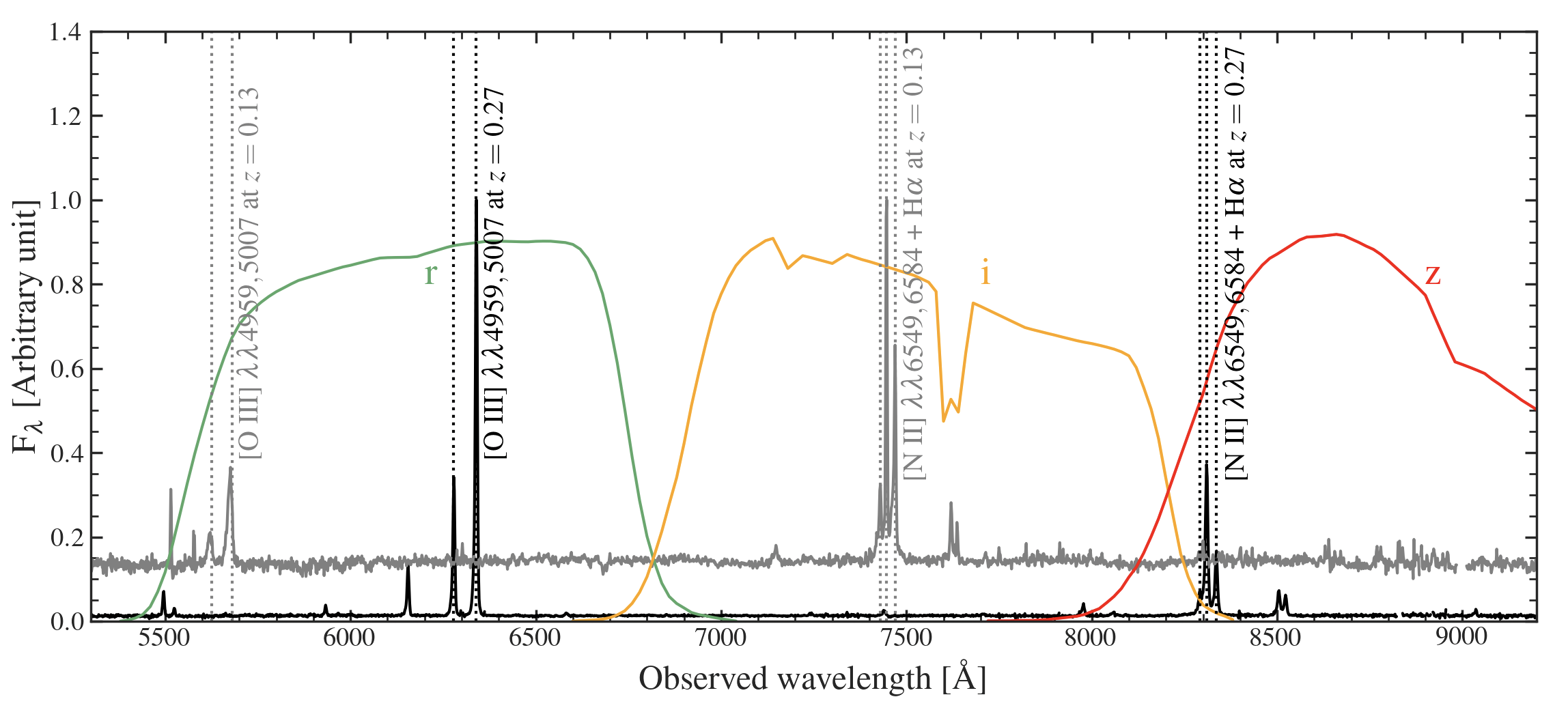
Figure 2: Spectra of SDSS J$092729.11+193640.1$ at $z=0.13$ (gray) and SDSS J$162209.41+352107.5$ at $z=0.27$ (black). The green, yellow, and red lines represent the area normalized transmission curve of $r$, $i$, and $z$ bands, respectively. The vertical dashed lines indicate the location of emission lines.

Because the transmission curves and bandwidth are different in all $riz$ bands, the $z$-band and $i$-band images are scaled to match the continuum in the $r$-band image. Generally, the ratio of the stellar continuum in the $r$ band to that in the $i$ or $z$ band can be determined by convolving the spectrum with the transmission curves of the corresponding filters. However, the wavelength coverage of the spectra is up to 9200 Å, while it is 11,000 Å for the $z$ band. Instead of using the observed spectra, We fit them with the power law and use the best-fit power-law spectrum to convolve with the filters. The ratio ($\Theta$) of the continuum in the $r$ band to that in the $i$- or $z$-band is thus written as

$$\Theta=\frac{\int\lambda^{\beta}T_{r}\lambda\;d\lambda}{\int\frac{T_{r}}{\lambda}d\lambda}\frac{\int\frac{T_{i,z}}{\lambda}d\lambda}{\int\lambda^{\beta}T_{i,z}\lambda\;d\lambda}$$ (1)

where $T_{r}$ and $T_{i,z}$ are the transmission curves of the $r$ and $i$ or $z$ bands, respectively and $\beta$ is the best-fit spectral index.

3.2 The point spread function (PSF) matching

We reconstructed the PSF model of each image using the psField files from the SDSS Science Archive Server (SAS). In the case of the continuum images, we adopted the PSF model in the filter originally used to create the continuum image (i.e., $i-$ or $z-$ band). We homogenized the PSF size of both $r-$band and continuum images using the $2$-dimensional Gaussian kernel to obtain the target FWHM of $1.93$″, the maximum PSF size of all images. Figure 3 shows an example of the PSF matching between $r-$band and $z-$band images. The original FWHM of the examples $r-$band and $z-$band images are $1.71\arcsec$ and $1.64\arcsec$, respectively. The top panel illustrates that the images can be oversubtracted without the PSF matching. In this study, we keep the maximum residual below 10% of the peak of the target PSF by adjusting the width of the Gaussian kernel.

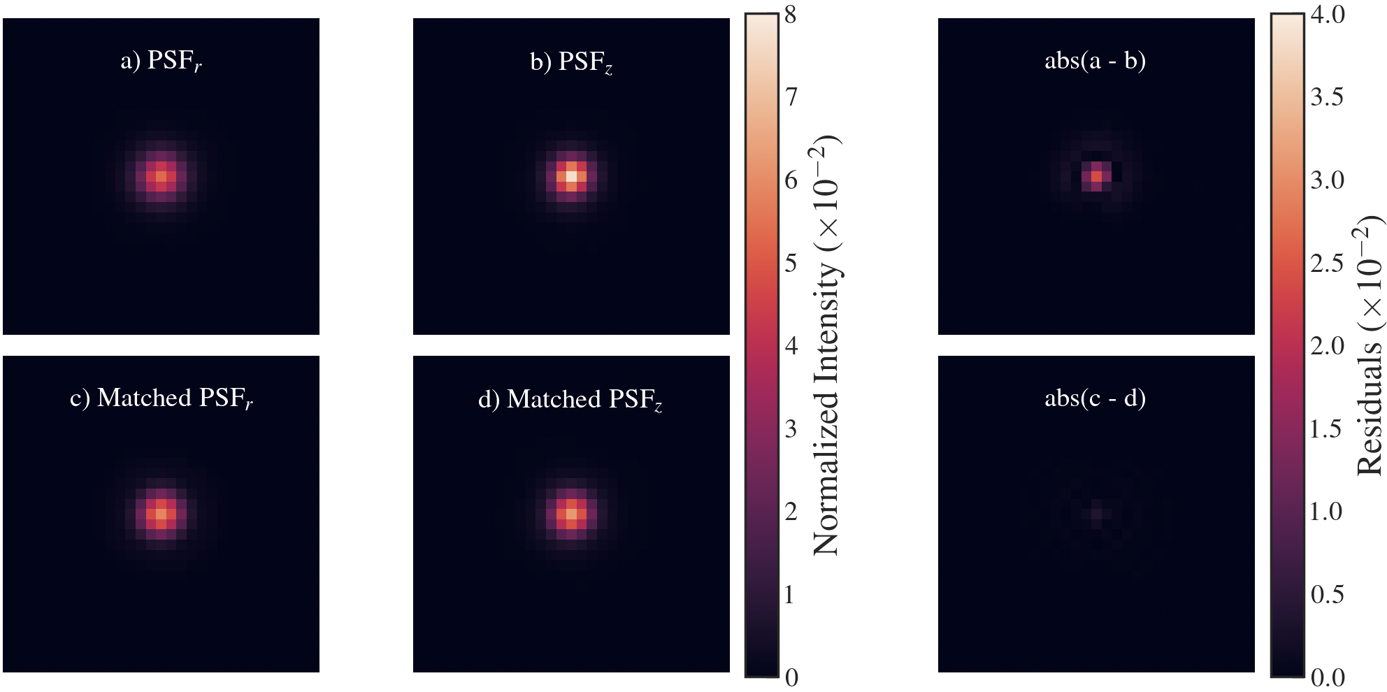
Figure 3: Example of the PSF models of the $r-$band image (left), the $z-$band image (middle), and the residual (right). The colorbar represents the normalized intensity such that the sum equals unity. The top and bottom panels show the PSF models before and after the matching using the Gaussian kernel, respectively.

3.3 Construction of [O III] images

After the PSF matching, we align images from different bands according to their WCS headers. The continuum images are adjusted to match the position in the $r$ band and then subtracted from the $r-$band image. The emission-line image contains all emission lines falling into the $r$ band. Although the [O III] emission line is normally the strongest, the contribution of the other lines in the emission-line image could cause an overestimation in [O III] area measurement. We calculated the ratio of [O III] emission line to the total fluxes from all emission lines in the $r$ band (hereafter called $\gamma_{5007}$) from the spectrum of each object. The $\gamma_{5007}$ was used to scale the emission-line images to the [O III] emission images. We also corrected the effects of the cosmological dimming and transmission curves as the objects are slightly at different redshifts and their [O III] emission falls into different parts of the $r$-band filter. Ultimately, the intensity of the [O III] $\lambda$5007 image ($I_{\mathrm{[O\;III]}}$) can be calculated from the intensity of the emission-line image ($I_{em}$) as follows

$$I_{\mathrm{[O\;III]}}=\frac{\gamma_{5007}\times(1+z)^{4}\times c}{T_{r,5007}\times\lambda_{\mathrm{obs},5007}}\times{\int\frac{T_{r}}{\lambda}d\lambda}\times I_{em}$$ (2)

where $\gamma_{5007}$ and $\lambda_{\mathrm{obs},5007}$ are the flux ratio of [O III] $\lambda$5007 to total in the $r$ band and the observed wavelength of [O III] $\lambda$5007 . $T_{r,5007}$ and $T_{r}$ are the transmission function of the $r$-band filter at $\lambda_{\mathrm{obs},5007}$ and any wavelength $\lambda$, respectively. $c$ is the speed of light in vacuum.

3.4 Isophotal area of [O III] $\lambda 5007$ emission

We measured the depth of [O III] images by fitting the noise distribution of each emission-line image. A histogram of $1\sigma$ noise level of all [O III] images is shown in Figure 4. The median of 1$\sigma$ noise ($\sigma_{\mathrm{med}}$) is $7.0\times 10^{-16}$ erg s^-1 cm^-2 arcsec^-2. We adopted $2\sigma_{\mathrm{med}}$ ($1.4\times 10^{-15}$ erg s^-1 cm^-2 arcsec^-2) as a flux limit in measuring the isophotal area of the target in the [O III] images. To avoid noise contamination in the area measurement, we excluded $127$ objects with the [O III] images showing $1\sigma$ noise levels higher than $2\sigma_{\mathrm{med}}$ marked by the dashed line in Figure 4. This isophotal threshold goes deeper than $3\times 10^{-15}$erg s^-1 cm^-2 arcsec^-2 adopted by Sun et al. (2018) using broadband images from the Subaru/HSC. However, it is shallower than the typically used value of $1\times 10^{-15}$ erg s^-1 cm^-2 arcsec^-2 adopted in other studies (Liu et al., 2013; Hainline et al., 2013) using IFU/long-slit spectroscopy to detect [O III] images.

To avoid the possible emission from nearby galaxies or foreground stars, we only considered the emission whose center is located within $5^{\prime\prime}$ ($11.6-24.2$ kpc) from the center of the stellar continuum. Notably, this method possibly excludes flickering AGNs that do not show central emission but extended light echo at a larger distance due to the past ionization (Schawinski et al., 2015).

The uncertainty in the [O III] area was determined by a set of one hundred Monte Carlo simulations. We randomly added Gaussian noise with 1$\sigma$ fluctuation into the [O III] image. For objects with $\sigma<\sigma_{\mathrm{med}}=1.4\times 10^{-15}$ erg s^-1 cm^-2 arcsec^-2  we alternately inserted the noise of $\sigma_{\mathrm{med}}$. The [O III] area of noisy images are measured the same way as the original [O III] images. The standard deviation of the noise-added images is adopted as the uncertainty of the area denoted as $\sigma_{\mathrm{A}}$.

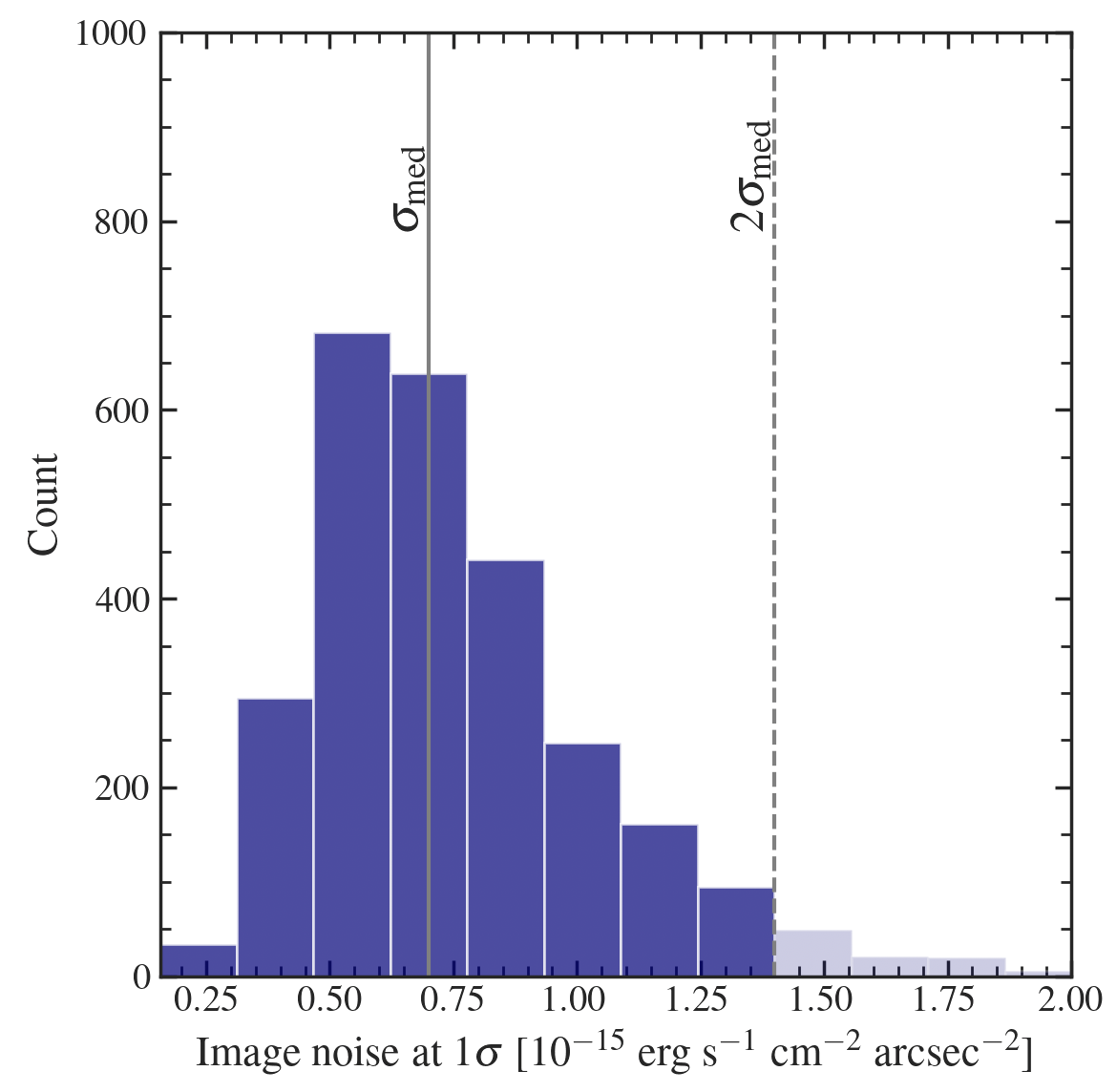
Figure 4: The noise distribution of $2{,}724$ [O III] emission line images of $2{,}724$ samples. The median noise $\sigma_{\mathrm{med}}$ of $7.0\times 10^{-16}$ erg s^-1 cm^-2 arcsec^-2 is illustrated by the solid line, while the dashed line shows $2\sigma_{\mathrm{med}}$ level. The shaded histograms show $127$ samples with $\sigma>2\sigma_{\mathrm{med}}$, which are removed from further discussion.

4 Measurement of [O III] kinematics

The gas kinematics in the NLR are examined via the [O III] $\lambda\lambda$4959,5007 emission lines from the SDSS integrated spectra. We firstly removed the stellar continuum from the spectra. The stellar templates are constructed using the MILES-based models by Vazdekis et al. (2010). We assumed the Salpeter (1955) initial mass function (IMF), 6 steps of metallicities, [Z/H] = [$-1.71,-1.31,-0.71,-0.40,0.00,0.22$], and 26 age steps equally spaced from $1.0$ to $12.6$ Gyrs. We used the penalized Pixel-Fitting package (pPXF, Cappellari & Emsellem, 2004) to perform the stellar continuum fitting and subtracting.

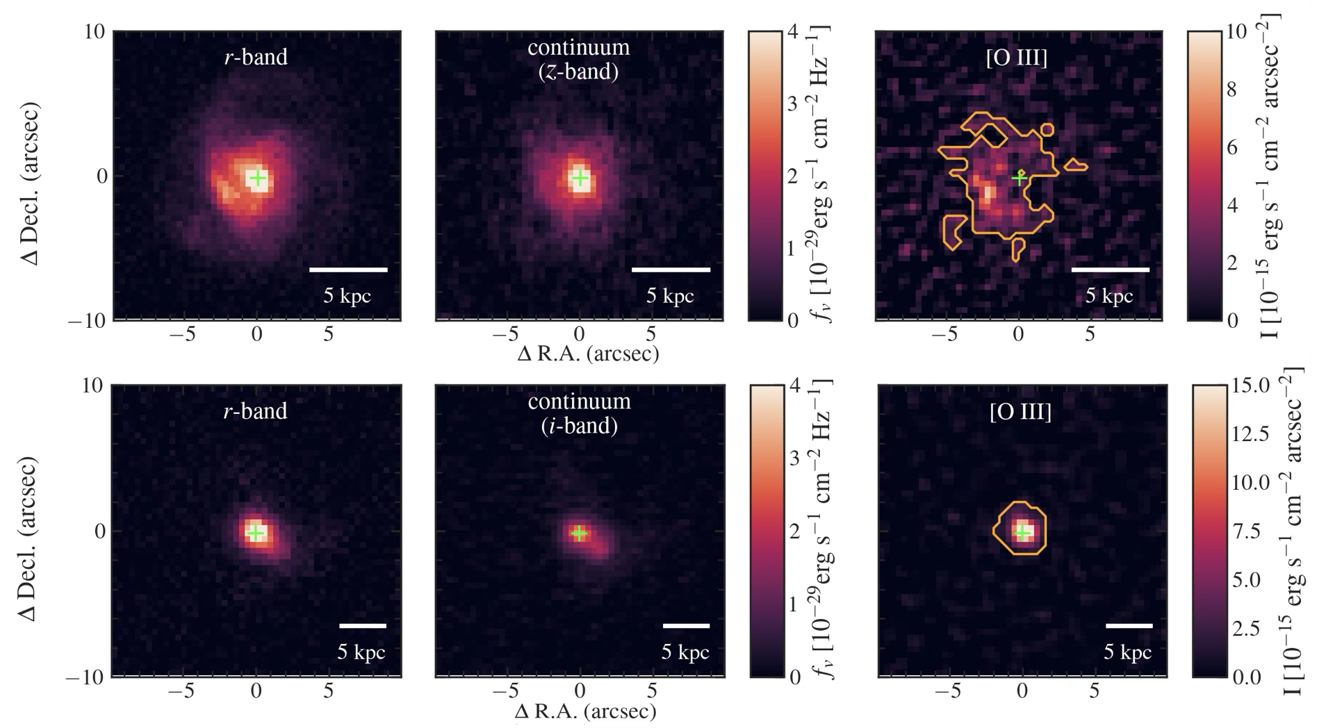
Figure 5: [O III] $\lambda$5007 image construction of two examples: SDSS J$092729.11+193640.1$ at $z=0.13$ (top) and SDSS J$162209.41+352107.5$ at $z=0.27$ (bottom). The image size is $20\arcsec\times 20\arcsec$. The left, middle, and right panels show the original $r$-band, constructed continuum, and resulting [O III] images, respectively. The green crosses mark the center in the continuum image. The colormap in the $r$-band and continuum images represents flux density in a unit of erg s^-1 cm^-2 Hz^-1. The right panel shows the [O III] image in a unit of $10^{-15}$ erg s^-1 arcsec^-2. The contour encloses the isophote area down to $1.7\times 10^{-15}$ erg s^-1 cm^-2 arcsec^-2 (see Section 3.4).

After the stellar continuum subtraction, the [O III] $\lambda\lambda$4959,5007 emission lines were fitted with Gaussian profiles using the MPFIT package (Markwardt, 2009), which was translated into PYTHON version by Mark Rivers. The [O III] doublets are assumed to share the same kinematics (i.e., identical systemic velocity and line width). Each emission line was fitted twice with a single and double Gaussian profile. In the case of single Gaussian fitting, the width of the Gaussian profile must be larger than the spectral resolution of SDSS spectra ($69$ km s^-1). In the case of double Gaussian fitting, we constrained the core and wing components to center within $\pm 180$ km s^-1 and $\pm 500$ km s^-1 of the systemic velocity, respectively. The peak of each component must be higher than the noise level, i.e., the amplitude-to-noise ratio (A/N) must be larger than $3$ (Woo et al., 2016).

We determined the Bayesian information criterion (BIC) for each fitting to see if the [O III] $\lambda\lambda$4959,5007 emission lines are fitted better with a single or double Gaussian profile. The model with a lower BIC value is generally chosen over the other. We computed $\Delta\mathrm{BIC}$ as $(\chi^{2}_{\mathrm{1}}+k_{\mathrm{1}}\ln n)-(\chi^{2}_{\mathrm{2}}+k_{\mathrm{2}}\ln n)$, where $\chi^{2}_{\mathrm{1,2}}$ are the total $\chi^{2}$ for the single and double Gaussian profile, respectively, $k_{\mathrm{1,2}}$ are the number of free parameters of each profile, and $n$ is the number of data points. The double Gaussian profile was adopted for the samples with $\Delta\mathrm{BIC}>10$ (Swinbank et al., 2019).

We determined the [O III] velocity dispersion ($\sigma_{\mathrm{[O\;III]}}$) from the non-parametric [O III] linewidth ($\Delta\lambda$), calculated from the best fitting profile as follows.

$$\Delta\lambda=\sqrt{\frac{\int\lambda^{2}f_{\lambda}\,d\lambda}{\int f_{\lambda}d\lambda}-\lambda_{\mathrm{cen}}^{2}},$$ (3)

where $\lambda_{\mathrm{cen}}=\int\lambda f_{\lambda}d\lambda\;/\int f_{\lambda}d_{\lambda}$ is the flux-weighted center of the line profile and $c$ is the speed of light in vacuum. The [O III] velocity shift ($\Delta$V${}_{\mathrm{[O\;III]}}$) is translated from the shift of $\lambda_{\mathrm{cen}}$ from the center of the emission line.

5 RESULTS

5.1 Spatial Extent of [O III] emission

Figure 5 shows the [O III] image construction of two samples whose spectra are illustrated in Figure 2. The top panel is SDSS J$092729.11+193640.1$ at $z=0.13$, whose continuum image was constructed from the $z$-band image, while the continuum image of SDSS J$162209.41+352107.5$ at $z=0.27$ in the bottom panel was created from the $i$-band image. The [O III] image of both objects shows a different morphology than the continuum one. It is suggested that using different images to construct the continuum image does not affect the result. In addition to 127 objects with noisy [O III] images, we excluded another 588 samples from the analysis as there is no [O III] emission in the subtracted images. We have $2{,}009$ AGNs to investigate the [O III] extension.

Figure 6 shows the overall relation between [O III] area and [O III] luminosity of $2{,}009$ AGNs. The [O III] areas range from $3.7$ kpc² to $224$ kpc², while the [O III] luminosity is approximately L${}_{\mathrm{[O\,III]}}$$\sim 10^{40-43}$ erg s^-1. The [O III] area tends to increase with increasing [O III] luminosity, especially for objects at $z=0.26$. The objects at $z=0.26$ are shown separately as their continuum images were constructed using the $i$-band instead of the $z$-band used at the lower redshifts (see Section 3.1). At $z>0.26$, the samples tend to exhibit larger [O III] area and higher L${}_{\mathrm{[O\,III]}}$ than those at $z<0.26$. Based on the Kolmogorov-Smirnov (KS) test, we can reject the null hypothesis that the distributions of the [O III] area and luminosity of the objects at $z<0.26$ and at $z>0.26$ are drawn from the same populations at the p-value of $3.47\times 10^{-6}$ and $0.01$, respectively.

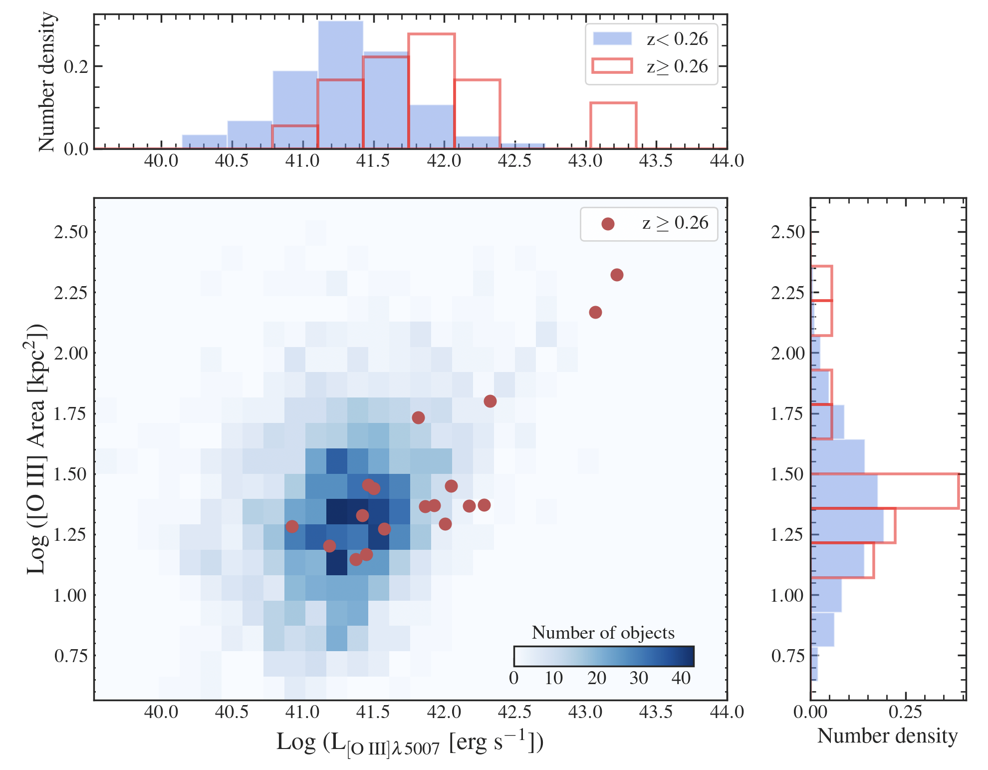
Figure 6: [O III] area-luminosity relation of $2{,}009$ AGNs. The density map in the middle panel indicates the number of samples at $z<0.26$. The red dots are samples at $z\geq 0.26$. The top and right panels show the distributions of [O III] area and [O III] luminosity, respectively. Shaded and open histograms represent samples at $0.13<z<0.26$ and at $z\geq 0.26$, respectively.

5.2 [O III] area-AGN luminosity relation

Figure 7 illustrates the relationship between the [O III] areas and luminosities with the velocity dispersion in the colorbar. Objects with higher luminosities tend to show larger [O III] area and higher velocity dispersions. In the left panel, we plot the relation between [O III] area and [O III] luminosity without separating the samples at $z>0.26$ as plotted in Figure 6. Based on Pearson’s correlation coefficient, the [O III] area is moderately correlated with the [O III] luminosity ($r\sim 0.33$, $p<0.001$). The correlation can be written as $\log(\mathrm{[O\,III]\ Area})=(0.20\pm 0.01)\log(L_{\mathrm{[O\,III]}})-7.02$. The right panel shows the plot between the [O III] area and the bolometric luminosity computed from the rest-frame $15\mu m$ luminosity of $1{,}945$ subsamples with the WISE detections (see Section 2.3). The best-fit correlation is $\log(\mathrm{[O\,III]\ Area})=(0.27\pm 0.02)\log(L_{\mathrm{bol,15\mu m}})-10.46$, with the Pearson’s coefficient of $r\sim 0.31$ at $p<0.001$.

We compare our results with the study by Sun et al. (2018) using HSC broadband images to map the [O III] images in $300$ type-2 AGNs. They have established the [O III] Area - luminosity relation with a slope of $0.62\pm 0.01$ and the Pearson’s $r\sim 0.68$ ($p<0.01$). Their correlation is significantly stronger than those found in this work. However, it is possibly due to the difference in the threshold used to determine the isophotal area. Sun et al. (2018) adopted the rest-frame isophotal threshold of $3\times 10^{-15}$erg s^-1 cm^-2 arcsec^-2, while we used $1.7\times 10^{-15}$erg s^-1 cm^-2 arcsec^-2(Section 3.4). They showed the result of using the lower isophotal cut of $1\times 10^{-15}$erg s^-1 cm^-2 arcsec^-2, yielding a much flatter slope of $0.2$, which is comparable to our result. In addition, we noticed that they have a higher fraction of high-luminosity samples with L_bol,15μm$>10^{45}$ erg s^-1 that could affect the best-fit slope in a regression analysis. Nevertheless, our goal in this study is to justify the impact of outflows on the size-luminosity relation, and even so, our result could statistically verify that the size of the [O III] emission is typically large among high-luminosity AGNs, which agrees well with previous studies (Liu et al., 2013; Hainline et al., 2013; Sun et al., 2017). We make further discussions on the size-luminosity relation in Section 6.2.

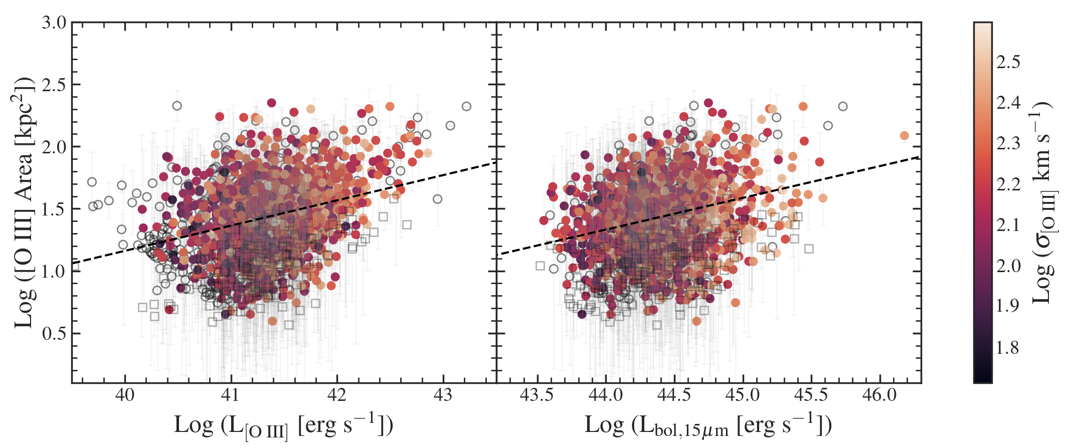
Figure 7: The [O III] area as a function of [O III] luminosity ($L_{\mathrm{[OIII]}}$); left) and bolometric luminosity ($L_{\mathrm{bol,15\mu m}}$; right). Solid circles are $2{,}009$ (left) and $1{,}945$ (right) AGNs, while their colors indicate the velocity dispersion of [O III] emission ($\sigma_{\mathrm{[O\;III]}}$). Gray open circles represent objects with no $\sigma_{\mathrm{[O\;III]}}$(Section 5.3). The dashed lines show the best-fit power laws from a linear regression model. The error bars indicate the standard deviation ($\sigma_{\mathrm{A}}$) in the area measurement

(See Section 3.4).

5.3 [O III] spectral profiles and outflow signature

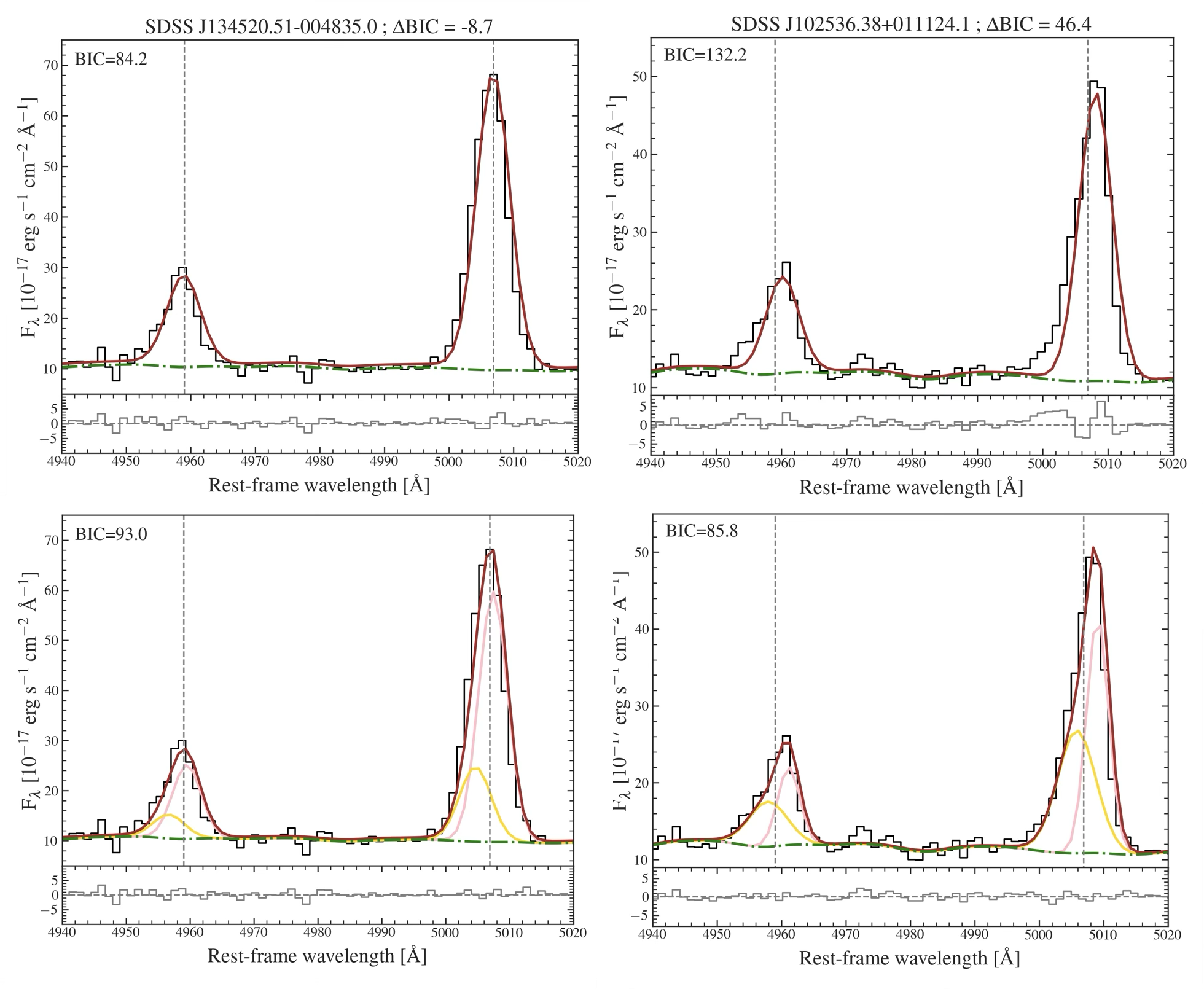
Figure 8: [O III] $\lambda\lambda$4959,5007emission lines with the fitting residual of SDSS J$134520.51-004835.0$ at $z=0.17$ (left) and SDSS J$102536.38+011124.1$ at $z=0.18$ (right). The black solid line shows the original SDSS spectrum. The top and bottom panels show the case of using single and double Gaussian models, respectively. The red solid and green dash-dotted lines show the best-fit [O III] emission lines and the stellar continuum model, respectively. The pink and yellow lines in the bottom panel represent the core and the wing components, respectively. The BIC value is also shown at the top left corner of each panel. The residual plots are displayed below each subplot.

Two examples of [O III] emission-line fittings are shown in Figure 8. The spectrum of each object is fitted with single and double Gaussian models. The best-fit model is then determined by the $\Delta\mathrm{BIC}$ criterion, as explained in Section 4. Basically, the model with the lowest value of BIC is preferred. In the left panel, the [O III] emission line of SDSS J$134520.51-004835.0$ at $z=0.17$ is better fitted with a single Gaussian profile, which has a lower BIC than the double Gaussian model. The $\Delta\mathrm{BIC}$ in this case is smaller than 10 ($\Delta\mathrm{BIC}=-8.7$). On the other hand, the double Gaussian profile is chosen in the case of SDSS J$102536.38+011124.1$ (right panel). The double Gaussian model better describes the [O III] profile, with $\Delta\mathrm{BIC}>10$. The wing component is relatively strong compared to the core component, with a flux ratio between both components of $0.90$, making the total line profile look asymmetrical. With this fitting procedure, we obtained $916$ and $629$ objects with single and double Gaussian profiles, respectively. The remaining $464$ objects were excluded due to their low spectral quality, i.e., more than $80\%$ of the flux density have the S/N$\leq 8$ in the wavelength range of the [O III] fitting.

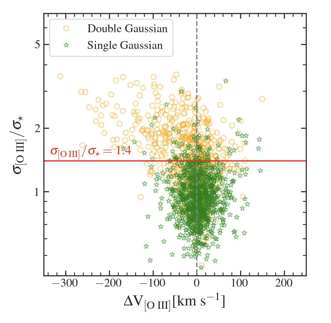
Figure 9: The ratio of [O III] velocity dispersion to stellar velocity dispersion versus velocity shift of $1{,}545$ objects. Yellow circles and green stars mark samples with the double-Gaussian and single-Gaussian profiles in their [O III] emission lines, respectively. The red line marks the value of $\sigma_{\mathrm{[O\;III]}}$/$\Delta$V${}_{\mathrm{[O\;III]}}$$=1.4$ used to select sample with outflows (Section 5.3)

Several methods are used to identify outflow signatures in the galaxy based on the [O III] emission-line profile, one of which is the existence of the wing component (e.g., Wylezalek et al., 2018; Perna, M. et al., 2019; Zheng et al., 2023). However, the spectral fitting is sensitive to the spectral data quality. We may miss gas outflowing samples whose [O III] emission line is best fitted with the single-Gaussian [O III] profile due to low S/N ratios. In this study, we assume that the observed velocity dispersion of the [O III] emission line is caused by gravitational potential from the host galaxy and the non-gravitational component, which is interpreted as as outflow signature. That is

$$\sigma_{\mathrm{[O\;III]}}^{2}=\sigma^{2}_{\mathrm{gr}}+\sigma^{2}_{\mathrm{non-gr}},$$ (4)

where $\sigma_{\mathrm{[O\;III]}}$ represents the observed [O III] velocity dispersion calculated from the best fitting Gaussian profile using Eq.3. The $\sigma_{\mathrm{gr}}$ and $\sigma_{\mathrm{non-gr}}$ denote the velocity dispersion of the gravitational and non-gravitational components, respectively. We adopted the stellar velocity dispersion to trace the strength of the gravitational potential, that is $\sigma_{\rm gr}=\sigma_{\star}$. We classified the samples with $\sigma_{\mathrm{[O\,III]}}/\sigma_{\star}>1.4$ as having the outflow signature. The $\sigma_{\mathrm{[O\,III]}}/\sigma_{\star}=1.4$ threshold is where the non-gravitational and gravitational components contribute equally to the observed [O III] emission.

Figure 9 shows the $\sigma_{\mathrm{[O\;III]}}$$/\sigma_{\star}$ ratio versus velocity shift ($\Delta$V${}_{\mathrm{[O\;III]}}$) of the samples. Generally, the $\sigma_{\mathrm{[O\;III]}}$$/\sigma_{\star}$ ratio tends to increase toward the negative [O III] velocity shift. The samples with outflow signature selected by our $\sigma_{\mathrm{[O\,III]}}/\sigma_{\star}>1.4$ threshold are not only those whose [O III] emission lines were best fitted with the double Gaussian profile, but also the samples with the best-fit single Gaussian [O III] emission or with the low [O III] velocity shift. For the galaxies with low dust extinction, it is possible that the receding component of biconical outflow can be detected and causes the lower estimation of the [O III] velocity shift (Woo et al., 2016). As a result, we finally have $621$ and $924$ samples with and without the signature of the outflows, respectively.

5.4 The impact of outflows on the spatial extent of the [O III] region

In this section, we investigate whether the size of the [O III] emission depends on the presence of gas outflows. We revisit the area-bolometric luminosity, as illustrated in Figure 10. The samples are now separated between having and not having outflows. The objects with outflows tend to have higher bolometric luminosity compared to those without outflows. Using the KS test, we can reject the null hypothesis that the bolometric luminosities of two subsamples are drawn from the same distribution ($p<0.01$). This suggests that outflows are more prominent among samples with high-luminosity AGNs. In contrast, [O III] area distributions of two subsamples are not statistically different. The correlation between [O III] areas and the [O III] velocity dispersion is very weak, with Pearson’s $r\sim 0.12$ and $p<0.001$. These results show that the presence of outflows does not affect the extension of the [O III] emission. As the correlation of the area-luminosity relation is much stronger than the area-velocity relation, this suggests that the photoionization by central AGNs seems to be the main driver of the spatial extent of the [O III] emission rather than the gas outflows.

Figure 10: The [O III] area-L_bol,15μm relations of AGNs with outflows (solid blue circles) and without outflows (open red circles). The solid blue and red lines show the best-fit relation of samples with and without outflows, respectively. The histograms along an x-axis and y-axis show the distributions of L_bol,15μm and [O III] areas between two subsamples. The error bars denote the median $1\sigma$ uncertainty of the [O III] areas and bolometric luminosity of two subsamples.

6 DISCUSSION

6.1 Detection of [O III] emission using broadband images

The [O III] images in this work are constructed based on the flux excess in the SDSS $r$-band images. Using the publicly available broadband data is an alternative inexpensive approach to increase the sample size in the study of the NLR. Previous studies have found a number of compact galaxies with strong [O III] emission lines giving distinct flux excess in the SDSS filters(Cardamone et al., 2009; Liu et al., 2022). With $\sim 1370$Å FWHM of the $r$-band filter, the [O III] emission line with the observed equivalent width EW([O III]) $\sim 100$Å  contributes to a magnitude excess of $\Delta m_{\mathrm{AB}}\sim 0.1$ in the emission-line image. Only galaxies with strong [O III] emission would be detected with this method.

As the value of EW([O III]) typically increases with the [O III] luminosity (Zakamska et al., 2003), it is expected that the number of objects with detected [O III] emission should increase with [O III] luminosity. The fraction of detecting [O III] emission in the broadband excess images or emission-line image is plotted as a function of [O III] luminosity in Figure 11. We compared three different isophotal criteria used in the area measurement: $1.7\times 10^{-15}$ erg s^-1 cm^-2 arcsec^-2 $(2\sigma_{\mathrm{med}})$, $2.25\times 10^{-15}$ erg s^-1 cm^-2 arcsec^-2 $(3\sigma_{\mathrm{med}})$, and $3\times 10^{-15}$ erg s^-1 cm^-2 arcsec^-2 (used in Sun et al. 2018). It is clearly seen from the figure that the detection fraction increases with the [O III] luminosity in all cases. However, the fraction reduces greatly when using the brighter isophotal threshold.

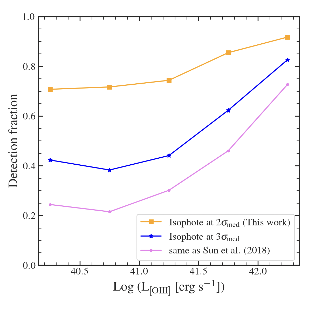
Figure 11: Detection fraction of [O III] emission using our broadband selection technique as a function of [O III] luminosity. Orange squares, blue stars, and magenta dots represent the rest-frame isophotal thresholds at $2\sigma_{\mathrm{med}}$, $3\sigma_{\mathrm{med}}$, and $3\times 10^{-15}$ erg s^-1 cm^-2 arcsec^-2, respectively.

6.2 Comparison of size-luminosity relation

We found that the [O III] area constructed from our broadband technique is correlated well with both [O III] and AGN luminosity consistent with previous studies (Hainline et al., 2013; Sun et al., 2017, 2018; Polack et al., 2024). Although many studies found a strong correlation between the size of the NLR and AGN luminosity in type-2 AGNs, the power-law slopes in the size-luminosity relation are not consistent with each other. The study using the Subaru/HSC broadband images by Sun et al. (2018) shows a strong correlation between the [O III] area and AGN luminosity with the power-law slope of $0.62\pm 0.10$. They measured the [O III] areas down to the rest-frame isophote of $3\times 10^{-15}$ erg s^-1 cm^-2 arcsec^-2. Hainline et al. (2013) and Sun et al. (2017) reported the shallower power-law slopes of $0.47\pm 0.02$ and $0.30$, respectively, when adopting a slightly deeper surface brightness cutoff at $10^{-15}$erg s^-1 cm^-2 arcsec^-2. Using the narrowband HST images, Polack et al. (2024) adopted a very faint isophotal threshold of $2\times 10^{-17}$erg s^-1 cm^-2 arcsec^-2and found a power-law slope of $0.39\pm 0.05$. The discrepancy in the derived power-law slopes is possibly due to different surface brightness thresholds used to determine the size of the [O III] emission. Using a brighter isophote would likely increase the slope of the size-luminosity relation.

To confirm this hypothesis, we compared our results with the study by Sun et al. (2018), who used the same broadband excess technique but with the Subaru/HSC images and significantly brighter isophotal threshold ($3\times 10^{-15}$ erg s^-1 cm^-2 arcsec^-2). To make a fair comparison, we adopted the same isophotal threshold and remeasured the [O III] area of our samples. The new [O III] area - L_bol,15μm relation is plotted in Figure 12 along with $300$ type-2 AGNs from Sun et al. (2018). The figure shows that the [O III] areas are consistent with each other at a given luminosity. The [O III] areas of our samples are less scattered at the low end of luminosity, while we have a significantly smaller number of samples at higher luminosity. With this new isophotal threshold for the [O III] area measurement, the correlation between the [O III] areas and luminosity of our samples becomes stronger with the Pearson’s $r\sim 0.52$, $p<0.001$ (cf. Section 5.2). This correlation strength becomes closer to $r\sim 0.68$ reported in Sun et al. (2018). We obtained a slightly steeper slope of $0.39\pm 0.02$ than using a shallower isophotal threshold in Section 5.2, but it is still shallower than the study by Sun et al. (2018). The difference in the slope might be due to the lack of high-luminosity samples (L_bol,15μm$>10^{45}$ erg s^-1), which could affect the result of the best-fit slope.

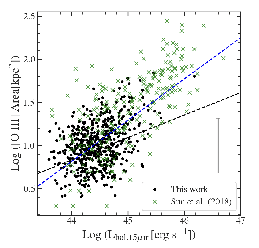
Figure 12: The [O III] isophotal area - bolometric luminosity relations of $860$ AGNs measured at the rest-frame isophote of $3\times 10^{-15}$ erg s^-1 cm^-2 arcsec^-2. The green x-symbols are 300 objects from Sun et al. (2018). The black dash line shows the size-luminosity relation of our samples. The blue dash line describes the size-luminosity relation from Sun et al. (2018). The gray error bar represents the median area uncertainty among our samples.

6.3 Influence of outflows on the gas clouds in the narrow-line regions (NLRs)

It is known that the ionization of gas in the NLR is mostly from the power-law radiation from the central AGNs (Evans & Dopita, 1985; Binette et al., 1996), sometimes with the contribution of fast shocks (Terao et al., 2016). The formation of the gas clouds in the NLRs is still unclear. One explanation is that they are already located inside the host galaxy and is photoionized by central AGNs. On the other hand, based on the radiation-driven fountain model by Wada et al. (2018), they showed that the AGN-driven outflow could also transfer the gas cloud from the central region to the outer part. Although the simulation is spatially-limited within $\sim 16$ pc from the nucleus, the more extended NLRs could be inferred from the model. The observational study by Joh et al. (2021) also supports the scenario that the gas clouds in the NLRs are originated in the nucleus, which are transferred by gas outflows as those gas have higher velocity dispersion and electron density compared to gas in the Hii region.

Our assumption is that if the gas in the NLRs is driven by outflows, their [O III] areas should be statistically different compared to samples without outflows, or at least the slope in the size-luminosity relation should be different. However, based on our results in Section 5.4, we found the same slopes in the [O III] Area-L_bol,15μm relations between two subsamples. The distribution of [O III] areas between two subsamples are also statistically consistent with each other. The slope is slightly steeper in case of samples with outflows. Nevertheless, there is still no statistical different in the area distribution between two subsamples with a $p\sim 0.17$ in the KS test and $p>0.25$ in the AD-test. It seems that the presence of gas outflows has no effects on the size of the [O III] emission.

In addition, we investigate the correlation of the area with the $\sigma_{\mathrm{[O\;III]}}$/$\sigma_{\star}$ ratio, which represents the strength of outflows. We have found that the ratios have much weaker correlation with the [O III] areas ($r\sim 0.1$) compared to the area-luminosity relation ($r\sim 0.3$). It is unlikely that the non-gravitational kinematics, or outflows alone could create more extended [O III] emission.

Our results do agree with previous spectroscopic studies, who found that the size of outflows is usually smaller than the size of the NLRs with the ratio of $0.22-0.72$ (Fischer et al., 2018; Kim et al., 2023; Polack et al., 2024). On the other hand, the recent study by Zheng et al. (2023) found that the size of gas outflows in the dwarf galaxy SDSS J$0228-0901$ is significantly larger than the NLR size, while the latter is still not deviated much from the standard slope of $\sim 0.42$ in the size-luminosity relation by Chen et al. (2019). It seems that the outflow kinematics should not affect the size of the NLRs, in which the AGN photoionization is often dominant at larger distance.

7 SUMMARY

This work investigates the impacts of gas outflows on the size of the NLRs, which is traced by the region of [O III] emission. We constructed the [O III] maps using the SDSS broadband images in the $r-$band filter, together with a continuum subtraction interpolated from the $i$ or $z$ band using the SDSS spectra. Our broadband technique can significantly enhance the sample size in the study of the NLRs compared to other spatially resolved techniques. Using a sample of type-2 AGNs at $0.13<z<0.34$ from the SDSS “emissionlinesport” table, there are $2{,}009$ objects with the detection of [O III] emission. Among all samples, there are $1{,}545$ objects with reliable [O III] emission line to determining the presence of outflows. The main results are summarized as follows.

1. Based on the rest-frame isophotal cut of $1.7\times 10^{-15}$ erg s^-1 cm^-2 arcsec^-2, our samples have the [O III] areas ranging from $3.7$ kpc² up to $224$ kpc². The [O III] areas seem to increase with the [O III] luminosity.

2. With the AGN bolometric luminosity calculated from the rest-frame $15\mu$m WISE luminosity, we obtain strong correlation of the [O III] area with [O III] luminosity and AGN bolometric luminosity with Pearson’s $r=0.33$ and $r=0.31$, respectively. We have established the area-luminosity relation as $\log(\mathrm{[O\,III]\ Area})=(0.27\pm 0.02)\log(L_{\mathrm{bol,15\mu m}})-10.46$.

3. By using the same isophotal level by Sun et al. (2018) in the area measurement, [O III] areas of our samples are consistent with their values. The correlation of the area-luminosity relation becomes stronger with Pearson’s $r$ of 0.52 which is close to their study. However, our predicted slope is still lower than their study. We believed that it is caused by a lack of the high-luminosity AGNs in our samples, which could affect the slope in the regression analysis.

4. As the [O III] luminosity increases, the [O III] velocity dispersion is higher and the velocity shift becomes more negative, suggesting the outflow kinematics is stronger in more luminous AGNs.

5. Using the strength of the non-gravitational component $\sigma_{\mathrm{[O\;III]}}/\sigma_{\star}$ ratio at $1.4$, we are able to classifiy $621$ and $924$ objects as having outflows and no outflows, respectively.

6. The size of NLR in AGNs with outflows is not statistically different from those with no outflows.

Our findings suggested that the extended [O III] emission is not influenced by outflow mechanisms, questioning the effectiveness of the mechanical mode of the AGN feedback to deplete the gas reservoir from the host galaxies in the moderate luminosity regime ($10^{43}-10^{46}$ erg s^-1).

8 Acknowledgements

This research project is supported by the National Research Council of Thailand (NRCT): N41A640219. S.Y. is supported by the Office of the Ministry of Higher Education, Science, Research, and Innovation through a research grant for new scholars (RGNS63-175).

References

- Aird et al. (2015) Aird, J., Coil, A. L., Georgakakis, A., et al. 2015, Monthly Notices of the Royal Astronomical Society, 451, 1892, doi: 10.1093/mnras/stv1062
- Alam et al. (2015) Alam, S., Albareti, F. D., Allende Prieto, C., et al. 2015, ApJS, 219, 12, doi: 10.1088/0067-0049/219/1/12
- Astropy Collaboration et al. (2013) Astropy Collaboration, Robitaille, T. P., Tollerud, E. J., et al. 2013, A&A, 558, A33, doi: 10.1051/0004-6361/201322068
- Baldassare et al. (2020) Baldassare, V. F., Dickey, C., Geha, M., & Reines, A. E. 2020, The Astrophysical Journal Letters, 898, L3, doi: 10.3847/2041-8213/aba0c1
- Baldwin et al. (1981) Baldwin, J. A., Phillips, M. M., & Terlevich, R. 1981, PASP, 93, 5, doi: 10.1086/130766
- Bertin & Arnouts (1996) Bertin, E., & Arnouts, S. 1996, A&AS, 117, 393, doi: 10.1051/aas:1996164
- Binette et al. (1996) Binette, L., Wilson, A. S., & Storchi-Bergmann, T. 1996, A&A, 312, 365
- Bower et al. (2006) Bower, R. G., Benson, A. J., Malbon, R., et al. 2006, MNRAS, 370, 645, doi: 10.1111/j.1365-2966.2006.10519.x
- Cappellari & Emsellem (2004) Cappellari, M., & Emsellem, E. 2004, PASP, 116, 138, doi: 10.1086/381875
- Cardamone et al. (2009) Cardamone, C., Schawinski, K., Sarzi, M., et al. 2009, Monthly Notices of the Royal Astronomical Society, 399, 1191, doi: 10.1111/j.1365-2966.2009.15383.x
- Carraro et al. (2020) Carraro, R., Rodighiero, G., Cassata, P., et al. 2020, Astronomy &; Astrophysics, 642, A65, doi: 10.1051/0004-6361/201936649
- Chen et al. (2019) Chen, J., Shi, Y., Dempsey, R., et al. 2019, Monthly Notices of the Royal Astronomical Society, 489, 855, doi: 10.1093/mnras/stz2183
- Chen et al. (2022) Chen, Z., He, Z., Ho, L. C., et al. 2022, Nature Astronomy, 6, 339, doi: 10.1038/s41550-021-01561-3
- Croton et al. (2006) Croton, D. J., Springel, V., White, S. D. M., et al. 2006, MNRAS, 365, 11, doi: 10.1111/j.1365-2966.2005.09675.x
- Evans & Dopita (1985) Evans, I. N., & Dopita, M. A. 1985, ApJS, 58, 125, doi: 10.1086/191032
- Fabian (2012) Fabian, A. 2012, Annual Review of Astronomy and Astrophysics, 50, 455, doi: https://doi.org/10.1146/annurev-astro-081811-125521
- Fischer et al. (2018) Fischer, T. C., Kraemer, S. B., Schmitt, H. R., et al. 2018, The Astrophysical Journal, 856, 102, doi: 10.3847/1538-4357/aab03e
- Greenwell et al. (2023) Greenwell, C., Gandhi, P., Stern, D., et al. 2023, Monthly Notices of the Royal Astronomical Society, 527, 12065, doi: 10.1093/mnras/stad3964
- Gültekin et al. (2009) Gültekin, K., Richstone, D. O., Gebhardt, K., et al. 2009, The Astrophysical Journal, 698, 198, doi: 10.1088/0004-637X/698/1/198
- Hainline et al. (2013) Hainline, K., Hickox, R., Greene, J., Myers, A., & Zakamska, N. 2013, The Astrophysical Journal, 774, doi: 10.1088/0004-637X/774/2/145
- Harikane et al. (2014) Harikane, Y., Ouchi, M., Yuma, S., et al. 2014, The Astrophysical Journal, 794, 129, doi: 10.1088/0004-637X/794/2/129
- Heckman et al. (2004) Heckman, T. M., Kauffmann, G., Brinchmann, J., et al. 2004, The Astrophysical Journal, 613, 109, doi: 10.1086/422872
- Hopkins & Quataert (2010) Hopkins, P. F., & Quataert, E. 2010, MNRAS, 407, 1529, doi: 10.1111/j.1365-2966.2010.17064.x
- Hopkins et al. (2007) Hopkins, P. F., Richards, G. T., & Hernquist, L. 2007, ApJ, 654, 731, doi: 10.1086/509629
- Izotov et al. (2011) Izotov, Y. I., Guseva, N. G., & Thuan, T. X. 2011, The Astrophysical Journal, 728, 161, doi: 10.1088/0004-637X/728/2/161
- Joh et al. (2021) Joh, K., Nagao, T., Wada, K., Terao, K., & Yamashita, T. 2021, Publications of the Astronomical Society of Japan, 73, 1152, doi: 10.1093/pasj/psab065
- Kang & Woo (2018) Kang, D., & Woo, J.-H. 2018, The Astrophysical Journal, 864, 124, doi: 10.3847/1538-4357/aad561
- Kewley et al. (2001) Kewley, L. J., Dopita, M. A., Sutherland, R. S., Heisler, C. A., & Trevena, J. 2001, ApJ, 556, 121, doi: 10.1086/321545
- Kim et al. (2023) Kim, C., Woo, J.-H., Luo, R., et al. 2023, The Astrophysical Journal, 958, 145, doi: 10.3847/1538-4357/acf92b
- Kormendy & Ho (2013) Kormendy, J., & Ho, L. C. 2013, ARA&A, 51, 511, doi: 10.1146/annurev-astro-082708-101811
- Lapi et al. (2006) Lapi, A., Shankar, F., Mao, J., et al. 2006, ApJ, 650, 42, doi: 10.1086/507122
- Liu et al. (2013) Liu, G., Zakamska, N. L., Greene, J. E., Nesvadba, N. P. H., & Liu, X. 2013, Monthly Notices of the Royal Astronomical Society, 430, 2327, doi: 10.1093/mnras/stt051
- Liu et al. (2022) Liu, S., Luo, A.-L., Yang, H., et al. 2022, The Astrophysical Journal, 927, 57, doi: 10.3847/1538-4357/ac4bd9
- Lynden-Bell (1969) Lynden-Bell, D. 1969, Nature, 223, 690, doi: 10.1038/223690a0
- Madau et al. (1996) Madau, P., Ferguson, H. C., Dickinson, M. E., et al. 1996, MNRAS, 283, 1388, doi: 10.1093/mnras/283.4.1388
- Magorrian et al. (1998) Magorrian, J., Tremaine, S., Richstone, D., et al. 1998, AJ, 115, 2285, doi: 10.1086/300353
- Markwardt (2009) Markwardt, C. B. 2009, in Astronomical Society of the Pacific Conference Series, Vol. 411, Astronomical Data Analysis Software and Systems XVIII, ed. D. A. Bohlender, D. Durand, & P. Dowler, 251, doi: 10.48550/arXiv.0902.2850
- Osterbrock & Ferland (2006) Osterbrock, D. E., & Ferland, G. J. 2006, Astrophysics of gaseous nebulae and active galactic nuclei
- Perna, M. et al. (2019) Perna, M., Cresci, G., Brusa, M., et al. 2019, A&A, 623, A171, doi: 10.1051/0004-6361/201834193
- Pillepich et al. (2019) Pillepich, A., Nelson, D., Springel, V., et al. 2019, Monthly Notices of the Royal Astronomical Society, 490, 3196, doi: 10.1093/mnras/stz2338
- Polack et al. (2024) Polack, G. E., Revalski, M., Crenshaw, D. M., et al. 2024, The Astrophysical Journal, 975, 129, doi: 10.3847/1538-4357/ad71c3
- Riffel et al. (2024) Riffel, R., Dahmer-Hahn, L. G., Vazdekis, A., et al. 2024, Monthly Notices of the Royal Astronomical Society, 531, 554, doi: 10.1093/mnras/stae1192
- Saglia et al. (2016) Saglia, R. P., Opitsch, M., Erwin, P., et al. 2016, ApJ, 818, 47, doi: 10.3847/0004-637X/818/1/47
- Salpeter (1955) Salpeter, E. E. 1955, ApJ, 121, 161, doi: 10.1086/145971
- Schawinski et al. (2015) Schawinski, K., Koss, M., Berney, S., & Sartori, L. F. 2015, Monthly Notices of the Royal Astronomical Society, 451, 2517, doi: 10.1093/mnras/stv1136
- Schawinski et al. (2007) Schawinski, K., Thomas, D., Sarzi, M., et al. 2007, MNRAS, 382, 1415, doi: 10.1111/j.1365-2966.2007.12487.x
- Scott et al. (2013) Scott, N., Graham, A. W., & Schombert, J. 2013, The Astrophysical Journal, 768, 76, doi: 10.1088/0004-637X/768/1/76
- Shin et al. (2019) Shin, J., Woo, J.-H., Chung, A., et al. 2019, The Astrophysical Journal, 881, 147, doi: 10.3847/1538-4357/ab2e72
- Silk & Rees (1998) Silk, J., & Rees, M. J. 1998, A&A, 331, L1, doi: 10.48550/arXiv.astro-ph/9801013
- Somerville & Davé (2015) Somerville, R. S., & Davé, R. 2015, Annual Review of Astronomy and Astrophysics, 53, 51, doi: 10.1146/annurev-astro-082812-140951
- Somerville et al. (2008) Somerville, R. S., Hopkins, P. F., Cox, T. J., Robertson, B. E., & Hernquist, L. 2008, Monthly Notices of the Royal Astronomical Society, 391, 481, doi: 10.1111/j.1365-2966.2008.13805.x
- Sun et al. (2017) Sun, A.-L., Greene, J. E., & Zakamska, N. L. 2017, The Astrophysical Journal, 835, 222, doi: 10.3847/1538-4357/835/2/222
- Sun et al. (2018) Sun, A.-L., Greene, J. E., Zakamska, N. L., et al. 2018, Monthly Notices of the Royal Astronomical Society, 480, 2302–2323, doi: 10.1093/mnras/sty1394
- Swinbank et al. (2019) Swinbank, A. M., Harrison, C. M., Tiley, A. L., et al. 2019, Monthly Notices of the Royal Astronomical Society, 487, 381, doi: 10.1093/mnras/stz1275
- Terao et al. (2016) Terao, K., Nagao, T., Hashimoto, T., et al. 2016, The Astrophysical Journal, 833, 190, doi: 10.3847/1538-4357/833/2/190
- Thomas et al. (2013) Thomas, D., Steele, O., Maraston, C., et al. 2013, Monthly Notices of the Royal Astronomical Society, 431, 1383, doi: 10.1093/mnras/stt261
- Torres-Papaqui et al. (2020) Torres-Papaqui, J. P., Coziol, R., Romero-Cruz, F. J., et al. 2020, The Astronomical Journal, 160, 176, doi: 10.3847/1538-3881/abae5a
- Vazdekis et al. (2010) Vazdekis, A., Sánchez-Blázquez, P., Falcón-Barroso, J., et al. 2010, MNRAS, 404, 1639, doi: 10.1111/j.1365-2966.2010.16407.x
- Wada et al. (2018) Wada, K., Yonekura, K., & Nagao, T. 2018, The Astrophysical Journal, 867, 49, doi: 10.3847/1538-4357/aae204
- Woo et al. (2016) Woo, J.-H., Bae, H.-J., Son, D., & Karouzos, M. 2016, The Astrophysical Journal, 817, 108, doi: 10.3847/0004-637X/817/2/108
- Wright et al. (2010) Wright, E. L., Eisenhardt, P. R. M., Mainzer, A. K., et al. 2010, AJ, 140, 1868, doi: 10.1088/0004-6256/140/6/1868
- Wylezalek & Zakamska (2016) Wylezalek, D., & Zakamska, N. L. 2016, MNRAS, 461, 3724, doi: 10.1093/mnras/stw1557
- Wylezalek et al. (2018) Wylezalek, D., Zakamska, N. L., Greene, J. E., et al. 2018, MNRAS, 474, 1499, doi: 10.1093/mnras/stx2784
- York et al. (2000) York, D. G., Adelman, J., John E. Anderson, J., et al. 2000, The Astronomical Journal, 120, 1579, doi: 10.1086/301513
- Yuma et al. (2017) Yuma, S., Ouchi, M., Drake, A. B., et al. 2017, ApJ, 841, 93, doi: 10.3847/1538-4357/aa709f
- Yuma et al. (2019) Yuma, S., Ouchi, M., Fujimoto, S., Kojima, T., & Sugahara, Y. 2019, The Astrophysical Journal, 882, 17, doi: 10.3847/1538-4357/ab2f87
- Yuma et al. (2013) Yuma, S., Ouchi, M., Drake, A. B., et al. 2013, Astrophys. J., 779, 53, doi: 10.1088/0004-637X/779/1/53
- Zakamska et al. (2003) Zakamska, N. L., Strauss, M. A., Krolik, J. H., et al. 2003, AJ, 126, 2125, doi: 10.1086/378610
- Zheng et al. (2023) Zheng, Z., Shi, Y., Bian, F., et al. 2023, Monthly Notices of the Royal Astronomical Society, 523, 3274–3285, doi: 10.1093/mnras/stad1642
- Zhuang & Ho (2020) Zhuang, M.-Y., & Ho, L. C. 2020, ApJ, 896, 108, doi: 10.3847/1538-4357/ab8f2e