Localizing Dynamically-Formed Black Hole Binaries in Milky Way Globular Clusters with LISA

Abstract

The dynamical formation of binary black holes (BBHs) in globular clusters (GCs) may contribute significantly to the observed gravitational wave (GW) merger rate. Furthermore, LISA may detect many BBH sources from GCs at mHz frequencies, enabling the characterization of such systems within the Milky Way and nearby Universe. In this work, we use Monte Carlo N-body simulations to construct a realistic sample of Galactic clusters, thus estimating the population, detectability, and parameter measurement accuracy of BBHs hosted within them. In particular, we show that the GW signal from $0.7\pm 0.7$, $2.0\pm 1.7$, $3.6\pm 2.3$, $13.4\pm 4.7$ BBHs in Milky Way GCs can exceed the signal-to-noise ratio threshold of $\rm SNR=30$, 5, 3, and 1 for a 10-year LISA observation, with $\sim 50\%$ of detectable sources exhibiting high eccentricities ($e\gtrsim 0.9$). Moreover, the Fisher matrix and Bayesian analyses of the GW signals indicate these systems typically feature highly-resolved orbital frequencies ($\delta f_{\rm orb}/f_{\rm orb}\sim 10^{-7}-10^{-5}$) and eccentricities ($\delta e/e\sim 10^{-3}-0.1$), as well as a measurable total mass when SNR exceeds $\sim 20$. Notably, BBHs with $\rm SNR\gtrsim 20$ can be confidently localized to specific GCs within the Milky Way, with an angular resolution of $\sim 10-100$ arc minutes. The detection and localization of even a single BBH in a Galactic GC would allow accurate tracking of its long-term orbital evolution, enable a direct test of the role of GCs in BBH formation, and provide a unique probe into the evolutionary history of Galactic clusters.

1 Introduction

The LIGO/Virgo/KAGRA (LVK) collaboration (e.g., The LIGO Scientific Collaboration et al., 2021) has detected approximately 100 extragalactic binary black holes (BBH) mergers (e.g., Abbott et al., 2023). However, the formation channels for these mergers remain unclear, with various proposed mechanisms potentially contributing, including isolated binary evolution (e.g., Belczynski et al., 2016; Stevenson et al., 2017; Eldridge et al., 2019); dynamical formation in galactic centers (Kocsis & Levin, 2012; Hoang et al., 2019; Stephan et al., 2019; Arca Sedda et al., 2023; Zhang & Chen, 2024), galactic fields (Michaely & Perets, 2019, 2020; Michaely & Naoz, 2022; Stegmann et al., 2024), globular clusters (GCs) (e.g., Rodriguez et al., 2016b; Fragione & Bromberg, 2019; Kremer et al., 2020), active galactic nuclei disks (Tagawa et al., 2021; Peng & Chen, 2021; Samsing et al., 2022; Muñoz et al., 2022; Gautham Bhaskar et al., 2023), hierarchical triple systems (Wen, 2003; Naoz, 2016; Hoang et al., 2018; Antonini & Gieles, 2020), and primordial black hole scenarios (Bird et al., 2016; Sasaki et al., 2016). A key challenge in distinguishing these channels arises from the large distances and limited sky localization accuracy of extragalactic BBH mergers (e.g., Vitale & Whittle, 2018), which prevent confident identification of specific host environments. On the other hand, the future Laser Interferometer Space Antenna (LISA) (Amaro-Seoane et al., 2017) will observe BBHs in a lower frequency band ($10^{-4}-10^{-1}~\rm Hz$), which potentially allows us to probe their earlier evolutionary stages in the local Universe and distinguish between different hosting environments (see, e.g., Barack & Cutler, 2004; Mikóczi et al., 2012; Robson et al., 2018; Chen et al., 2019; Hoang et al., 2019; Fang et al., 2019; Tamanini et al., 2020; Breivik et al., 2020; Torres-Orjuela et al., 2021; Wang et al., 2021; Xuan et al., 2021; Zhang et al., 2021; Naoz et al., 2022; Amaro-Seoane et al., 2022; Naoz & Haiman, 2023).

In particular, GCs are considered ideal places for the dynamical formation of mHz BBHs (Miller & Hamilton, 2002; Portegies Zwart & McMillan, 2002; Morscher et al., 2015; Rodriguez et al., 2015, 2016a; Samsing & D’Orazio, 2019; Samsing, 2018; D’Orazio & Samsing, 2018; Zevin et al., 2019; Kremer et al., 2019a; Gerosa et al., 2019; Vitale, 2021). For example, a large number of black holes (BHs) can form through stellar evolution in clusters (see, e.g., Kroupa, 2001; Morscher et al., 2015). Due to mass segregation, these BHs gradually sink to the cluster core on sub-gigayear timescales, leading to the formation of a BH-dominated central region (Spitzer, 1969; Kulkarni et al., 1993; Sigurdsson & Hernquist, 1993). In the BH-dominated core, dynamically hard BH binaries promptly form through three-body interactions and further harden through gravitational wave (GW) capture, binary-single, and binary-binary scattering events (Heggie, 2001; Merritt et al., 2004; Mackey et al., 2007; Breen & Heggie, 2013; Peuten et al., 2016; Wang et al., 2016; Arca Sedda et al., 2018; Kremer et al., 2018a; Zocchi et al., 2019; Zevin et al., 2019; Kremer et al., 2020; Antonini & Gieles, 2020). Collectively, these dynamical processes result in BBH merger events at an estimated rate of $\mathcal{R}_{0}\approx 7.2_{-5.5}^{+21.5}\mathrm{Gpc}^{-3}\mathrm{yr}^{-1}$ in the local universe (e.g., Rodriguez et al., 2016b; Kremer et al., 2020; Antonini & Gieles, 2020), potentially making a significant contribution to the total GW merger rate detected by the LVK.

Moreover, dynamically-formed BBHs in GCs can provide valuable information about their astrophysical environment. For example, BBH mergers in a dense stellar environment typically have non-negligible eccentricity (e.g., O’Leary et al., 2009; Thompson, 2011; Aarseth, 2012; Kocsis & Levin, 2012; Breivik et al., 2016; D’Orazio & Samsing, 2018; Zevin et al., 2019; Samsing et al., 2019; Martinez et al., 2020; Antonini & Gieles, 2020; Kremer et al., 2020; Winter-Granić et al., 2023; Rom et al., 2024), which could greatly enhance our understanding of their formation mechanisms (see, e.g., East et al., 2013; Samsing et al., 2014; Coughlin et al., 2015; Breivik et al., 2016; Vitale, 2016; Nishizawa et al., 2017; Zevin et al., 2017; Gondán et al., 2018a, b; Lower et al., 2018; Romero-Shaw et al., 2019; Moore et al., 2019; Abbott et al., 2021; The LIGO Scientific Collaboration et al., 2021; Zevin et al., 2021), improve parameter estimation accuracy (Xuan et al., 2023a), or help with detecting the presence of tertiary companions through eccentricity oscillations (Thompson, 2011; Antognini et al., 2014; Hoang et al., 2018; Stephan et al., 2019; Martinez et al., 2020; Hoang et al., 2020; Naoz et al., 2020; Stephan et al., 2019; Wang et al., 2021; Knee et al., 2022). Further, as shown by recent studies, many BBHs undergo a wide (semi-major axis $a\gtrsim 0.1\,\rm au$), highly eccentric (eccentricity $e\gtrsim 0.9$) progenitor stage before the final merger (see, e.g., Kocsis & Levin, 2012; Hoang et al., 2019; Xuan et al., 2023b; Knee et al., 2024), which can also have unique imprints on mHz GW detections (Xuan et al., 2024a, b).

In this work, we will explore the properties of dynamically-formed BBHs in Milky Way GCs, with a focus on their detectability and parameter measurement accuracy in the mHz GW detection of LISA. Particularly, previous studies have shown that LISA can detect a handful of BBHs formed through isolated binary channels in the Milky Way (see, e.g., Lamberts et al., 2018; Sesana et al., 2020; Wagg et al., 2022; Tang et al., 2024). On the other hand, with approximately 150 GCs in the Milky Way (e.g., Harris, 1996; Baumgardt & Hilker, 2018), we expect a significant number of dynamically-formed BBH sources from these clusters (see, e.g., Kremer et al., 2018a), for which more specific predictions of their population are still needed.

We highlight that the detection of even a single BH in Milky Way GCs would provide a direct test of the role of GCs in BBH formation, offering valuable insights into the relative contributions of different formation channels to the observed BBH population. Therefore, it is essential to create a realistic sample of globular clusters that harbor binary black holes in the Milky Way, which will enable us to constrain the underlying populations of black holes and BBHs in GCs and assess which specific Galactic globular clusters are most likely to host resolvable BBHs within the LISA frequency band.

This paper is organized as follows. In Section 2, we introduce the simulation of globular clusters (the CMC Cluster Catalog cluster model) used in this work. Next, we fit the simulated clusters to Galactic globular clusters, thus estimating the population of Galactic BBHs in GCs today. Based on the simulations, we estimate the number of BBHs detectable by LISA, their eccentricity and mass distributions (see Section 3.1), and which specific Galactic GCs are most likely to host these sources (see Section 3.2). Furthermore, we adopt the Fisher matrix and Bayesian analyses in Section 3.3, and assess the parameter measurement accuracy of BBHs in the Milky Way GCs. In Section 4, we summarize the results and discuss the astrophysical implications. Throughout the paper, unless otherwise specified, we set $G=c=1$.

2 Creating a mock Galactic sample

To assemble a realistic sample of globular cluster BBHs, we use the CMC Cluster Catalog cluster models of Kremer et al. (2020). This suite of models is computed using the Monte Carlo $N$-body dynamics code CMC, which includes the most up-to-date physics for studying the formation and evolution of BHs in dense clusters (for review, see Rodriguez et al., 2022). Each of the 148 independent simulations of this catalog models the gravitational dynamics and stellar evolution for each of the $N$ stars in the system, keeping track of various properties (e.g., masses, semi-major axis, eccentricity) of all BBHs present in the cluster from formation to present day. The CMC Cluster Catalog has been tested rigorously against observations of Galactic globular clusters and successfully reproduces global features like surface brightness profiles, velocity dispersion profiles, and color-magnitude diagrams (Rui et al., 2021) as well as specific compact object populations including millisecond pulsars (Ye et al., 2019), X-ray binaries (Kremer et al., 2019a), cataclysmic variables (Kremer et al., 2021), and connections to BBHs observed by LIGO/Virgo (Kremer et al., 2020).

For this study, we aim to predict which specific Galactic GCs are most likely to host resolvable LISA sources at present. In this case, we must identify a single “best-fit” model from the CMC Cluster Catalog for each observed Milky Way GC. The CMC Catalog models can be sorted into a three-dimensional grid in $M_{\rm cl}-Z-R_{\rm gc}$ space, where $M_{\rm cl}$ is the total cluster mass at present (set by our choice of initial $N=[2,4,8,16,32]\times 10^{5}$ stars), $Z=[0.01,0.1,1]\times Z_{\odot}$ is the cluster metallicity, and $R_{\rm gc}=[2,8,20]\,$kpc is the Galactocentric position in the Galaxy. For a given observed GC, we identify the appropriate $M_{\rm cl}-Z-R_{\rm gc}$ model bin based on that GC’s observed mass and metallicity values (taken from Harris, 2010). Each distinct $M_{\rm cl}-Z-R_{\rm gc}$ bin contains 4 models of varying initial virial radius, which determines the clusters’ final core and half-light radius. To find the single best-fit model, we identify the model in the appropriate $M_{\rm cl}-Z-R_{\rm gc}$ bin which has core radius at $t=12\,$Gyr closest to the observed core radius value (Harris, 2010). Once the best fit model is identified, we select a cluster age by randomly sampling from that model’s available time snapshot outputs in the range $8-13.7\,$Gyr (typically this consists of a sample of 10-50 snapshots per model). This range is intended to reflect the uncertainty in cluster ages at present. Once a cluster snapshot is selected, we then identify the number and properties of all BBHs present in the best-fit model at that time. By repeating these steps for each observed GC, we build a sample of the full population of BBHs present in each of the Milky Way’s GCs at present. We then repeat this full procedure ten times to assemble ten separate Galactic realizations (the random time snapshot draw enables us to create distinct ten distinct samples).

Once this population is assembled, we compute the gravitational wave strain for each of the individual BBHs predicted within each Galactic cluster at present. Component masses, semi-major axes, and eccentricities are obtained directly from our best-fit CMC snapshot and the source distance and position is simply the heliocentric distance of the GC of interest (Harris, 2010).

Figure 1 shows an example of the simulated BBH population in Milky Way GCs. In particular, we choose one representative Galactic realization from the best-fit result of the CMC Catalog, and plot the orbital frequency ($f_{\rm orb}$) and the peak GW frequency ($f_{\rm peak}$) of each BBH system (e.g., O’Leary et al., 2009):

$$f_{\rm peak}=f_{\rm orb}(1+e)^{1/2}(1-e)^{-3/2}\,.$$ (1)

We note that most of the dynamically-formed systems have non-negligible eccentricity. In this case, $f_{\rm peak}$ of the eccentric GW signal indicates the frequency of the peak GW power, which typically needs to be within the mHz band for LISA to detect the source. Furthermore, in Figure 1, we can estimate the eccentricity of each system by comparing $f_{\rm peak}$ and $f_{\rm orb}$ (see the dashed lines with $e=0.99,0.97,0.9,0.7,0.2,0$, from left to right). For example, a system with $f_{\rm peak}\sim f_{\rm orb}$ should have moderate eccentricity, and a system with $f_{\rm peak}\gg f_{\rm orb}$ is highly eccentric.

In Figure 1, we use different colors to represent the signal-to-noise ratio (SNR) of BBHs, which is estimated analytically by summing the contributions from all the harmonics of their GW signal (see, e.g., Peters & Mathews, 1963; Kocsis & Levin, 2012; Xuan et al., 2023b):

$${\rm SNR}^{2}=8h^{2}_{0}(a)\sum_{n}\frac{g(n,e)}{S_{n}(nf_{\rm orb})n^{2}}T_{\rm obs}\ ,$$ (2)

in which $n=1,2,3...$ represents the number of harmonics, $T_{\rm obs}$ is the observation time, and $h_{0}(a)=\sqrt{32/5}\,m_{1}m_{2}/(Ra)$ depends on the binary’s component mass $m_{1},\,m_{2}$, semi-major axis $a$, and distance $R$. Additionally, $S_{\mathrm{n}}(f)$ is the spectral noise density of LISA evaluated at GW frequency $f$ (we adopt the LISA-N2A5 noise model, see, e.g., Klein et al., 2016; Robson et al., 2019), and $g(n,e)$ can be evaluated using:

$$g(n,e) =\frac{n^{4}}{32}\left[\left(J_{n-2}-2eJ_{n-1}+\frac{2}{n}J_{n}+2eJ_{n+1}-J_{n+2}\right)^{2}\right.$$ (3)

$$\left.+\left(1-e^{2}\right)\left(J_{n-2}-2J_{n}+J_{n+2}\right)^{2}+\frac{4}{3n^{2}}J_{n}^{2}\right],$$

in which $J_{i}$ is the $i$-th Bessel function evaluated at $ne$.

We note that the estimation of $\rm SNR$ in Equation (2) is based on the sky-average power of GW emission. In reality, the inclination and sky location of the GW source will also affect the detected $\rm SNR$, making it different from the average value. Therefore, the value of SNR shown in Figure 1 should be understood as a heuristic estimation (in most cases, the variation in SNR caused by different inclinations is within an order of magnitude of the average value). For a detailed discussion, see the appendix of Xuan et al. (2023b).

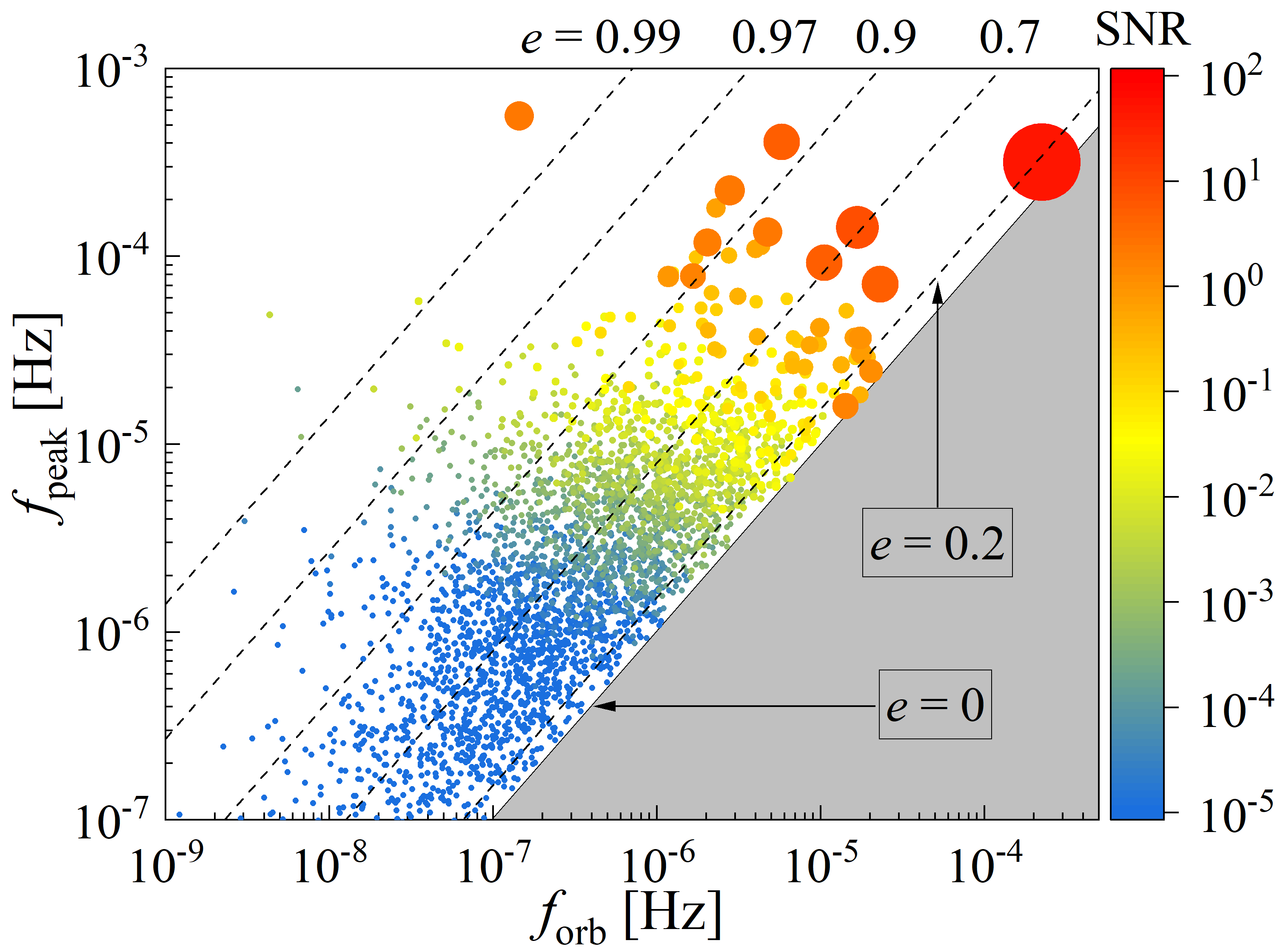
Figure 1: An example of simulated BBHs population in Milky Way GCs. Here, we plot the orbital frequency and peak GW frequency of BBH systems from a single realization of our simulated Milky Way GCs (see Equation (1)). The SNR of each BBH, estimated analytically using Equation (2) for a 5-year LISA observation, is represented by different colors. Detectable BBHs, based on their SNR, are highlighted with enlarged dots. Dashed lines indicate the eccentricity of BBHs in different regions, with $e=0.99,0.97,0.9,0.7,0.2,0$, from left to right. The simulated BBHs have an average component mass of $m_{1}=15.56~{\rm M_{\odot}},\,m_{2}=15.21~{\rm M_{\odot}}$ for in-cluster BBHs and $m_{1}=20.73~{\rm M_{\odot}},\,m_{2}=20.46~{\rm M_{\odot}}$ for ejected BBHs, but the mass of individual systems may vary.

As can be seen in Figure 1, the simulated orbital frequency and eccentricity of BBHs in Milky Way GCs distribute in a wide range of parameter space, with the majority of the binaries lying below the threshold of $\rm SNR=5$ for a 5-year LISA observation. However, there can be a handful of detectable sources with both moderate and high eccentricities. For example, we identified $3$ detectable sources in this realization, which have the orbital parameters of $f_{\rm orb}=2.24\times 10^{-4},1.67\times 10^{-5},5.79\times 10^{-6}$ Hz ($a=0.0075,0.048,0.079$ au) and $e=0.17,0.71,0.93$, respectively. Furthermore, there is a larger number ($\sim 20$) of highly eccentric BBHs in the region of $\rm SNR\sim 1-5$ (see the orange and yellow dots), which could be detected by LISA given a longer observation time, or contribute to a stochastic background of GW bursts (see, e.g., Xuan et al., 2024a).

3 Source Localization and Astrophysical Implications

3.1 Detectability and Eccentricity Distribution

Based on the simulation in Section 2, we computed the expected number of detectable BBHs formed in Milky Way GCs. In total, we expect the GW signal from $0.7\pm 0.7$, $2.0\pm 1.7$, $3.6\pm 2.3$, $13.4\pm 4.7$ BBHs to exceed the threshold of $\rm SNR=30$, 5, 3, and 1, respectively, for a 10-year observation of LISA . Furthermore, the simulation yields significant eccentricity for all the detectable BBH systems, with the eccentricity ranges from 0.167 - 0.994 for systems with $\rm SNR>3$, which is consistent with the expected eccentricity distribution of dynamically-formed binaries in GCs (see, e.g., Kremer et al., 2018a, for a LISA source expectations from Newtonian modeling of GCs).

We highlight that $\sim 50\%$ of the BBHs with $\rm SNR>5$ have high eccentricity in the detection ($e\gtrsim 0.9$); the fraction becomes even larger ($\sim 70\%$) for the population with $\rm SNR\sim 1-5$. This phenomenon reflects the highly eccentric nature of compact binary formation in a dense stellar environment. It also indicates that most of the GW signals from BBHs in Galactic GCs will be characterized by “repeated bursts” (Xuan et al., 2023b), for which the detectability and parameter extraction accuracy have been recently investigated (Xuan et al., 2024b).

The large fraction of highly eccentric BBHs can be understood analytically. In particular, the GW signal from eccentric binaries is made up of multiple harmonics, some of which have frequencies much higher than the binary’s orbital frequency (see, e.g., Equation (1)). Therefore, compared with circular BBHs, eccentric sources in GCs could enter the sensitive band of LISA with a much wider orbital separation $a$, when their $f_{\rm orb}$ is well below the mHz band. In other words, these eccentric binaries will be detected at the earlier evolution stages, with more extended lifetimes and larger number expectations than circular sources in the same frequency band. For example, highly eccentric, stellar mass BBHs can stay in the mHz GW band with a lifetime of (Peters & Mathews, 1963; Xuan et al., 2024a):

$$\tau_{\mathrm{ecc}}\sim\frac{3}{85\mu M^{2}}a^{4}\left(1-e^{2}\right)^{7/2}$$ (4)

$$\sim 1.17\times 10^{6}{\rm yr}\,\frac{2}{q(1+q)}\left(\frac{M}{20\rm M_{\odot}}\right)^{-3}\left(\frac{a}{1\rm au}\right)^{4}\left(\frac{1-e}{0.002}\right)^{\frac{7}{2}},$$

where $M=m_{1}+m_{2}$, $\mu=m_{1}m_{2}/(m_{1}+m_{2})$, and $q=m_{1}/m_{2}$. Note that this timescale is much longer than the merger timescale of a circular BBH system in mHz band (which typically lasts for $\sim 10^{3}-10^{5}$ years). Thus, these highly eccentric BBHs may dominate the population of BBHs in the local Universe, where their GW signals are strong enough to be identified.

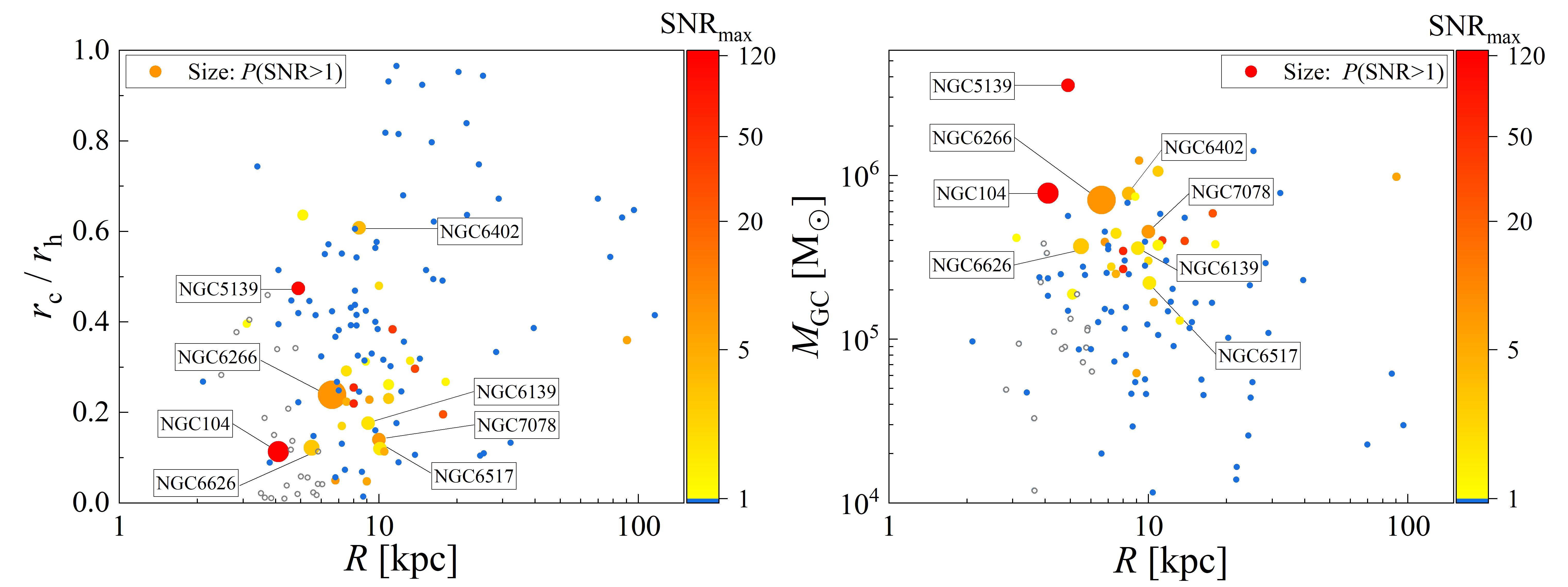
Figure 2: Properties of Milky Way globular clusters likely to host detectable BBHs in the mHz GW band. Here we adopt the simulation results of the BBH population in the Milky Way GCs, based on 10 realizations of in-cluster sources. The size of solid dots represents the expected probability for a cluster to host a BBH system with $\rm SNR>1$, $P({\rm SNR>1})$, and the color represents the maximum $\rm SNR$ of detectable BBHs, assuming a 10-year observation. Left Panel plots the distance $R$ (x-axis) against the ratio of the core radius to the half-light radius, $r_{c}/r_{h}$ (y-axis); Right Panel plots the distance $R$ (x-axis) against the estimated total mass $M_{\rm GC}$ of each globular cluster. The largest dot corresponds to the GC hosting 9 BBHs with $\rm SNR>1$ across the 10 realizations (i.e., an expected probability of $\sim 90\%$), while the smallest dots represent GCs hosting 1 BBH system with $\rm SNR>1$ (expected probability $\sim 10\%$). Solid blue dots represent GCs with no detectable BBHs (maximum $\rm SNR<1$), and hollow gray dots represent GCs without any BBHs in the simulation. We highlight the names of the top 8 GCs most likely to host detectable BBHs.

Additionally, binary mergers originating from GCs can be categorized into different types, based on their evolution history. On top of the binaries merging within the GC after dynamical interactions (in-cluster mergers), a significant fraction of BBHs can undergo multiple hardening encounters before being ejected from the cluster, eventually merging in the galactic field (ejected mergers; see, e.g., Downing et al., 2010; Rodriguez et al., 2016a, 2018; Kremer et al., 2019b). In our simulations, we find that in-cluster BBHs contribute approximately 0.7, 1.5, 2.2, and 5.8 GW sources, while the ejected population contributes around 0, 0.5, 1.4, and 7.6 GW sources above the thresholds of $\rm SNR=30$, 5, 3, and 1, respectively, for a 10-year LISA observation.

3.2 The Location of Gravitational Wave Sources

Next, we analyze which specific Galactic globular clusters are most likely to host resolvable BBHs, using the CMC Catalog from Kremer et al. (2020). In particular, we take the observational properties of Milky Way GCs following Harris (2010) (see dots in Figure 2), and choose the best-fit model in the CMC Catalog that matches the mass, metallicity, Galactic position, and core radius of each cluster (see Section 2). For each fitted cluster, we then compute the population properties of BHs and estimate their expectation of hosting a detectable BBH system.

The results are summarized in Figure 2. Specifically, Left Panel depicts the ratio of the clusters’ core radius to the half-light radius, $r_{c}/r_{h}$ (y-axis), versus their distance, $R$, from the detector (x-axis); Right Panel shows the estimated total mass of each cluster, $M_{\rm GC}$, against their distance $R$ (x-axis). The value of $r_{c}/r_{h}$ and $R$ are taken from Harris (2010), and the value of $M_{\rm GC}$ is adopted from Baumgardt & Hilker (2018). In Figure 2, the size of solid dots represents the expected probability for a cluster to host a BBH system with $\rm SNR>1$:

$$P({\rm SNR>1})=\frac{N_{{\rm SNR>1}}}{N_{\rm realization}}\ ,$$ (5)

where $N_{\rm realization}=10$ represents the total number of realizations for Milky Way GCs (see Section 2), and $N_{{\rm SNR>1}}$ represents the total number of BBHs with $\rm SNR>1$ in a GC, summed across all the realizations.

The color of dots in Figure 2 represents the detectability of their largest SNR GW source in the simulation, with colors ranging from yellow to red. Furthermore, we use solid blue dots to represent GCs with no detectable BBHs (maximum $\rm SNR<1$) and hollow gray dots to represent GCs without any BBHs in the simulation at all. In the Figure, we highlight the names of the eight fitted GCs that we predict are most likely to host detectable BBHs.

As illustrated in Figure 2, GCs with a high probability of hosting detectable BBHs tend to cluster within specific regions of the parameter space. Notably, we predict detectable BBHs are most likely to be resolved in GCs that are close in distance ($R\lesssim 10$ kpc), exhibit a small $r_{c}/r_{h}$ ($\sim 0.1-0.3$, indicative of denser, more dynamically-active GCs, see Left Panel), and have a large total mass (see Right Panel).

3.3 Astrophysical Implication

In this section, we first adopt the Fisher matrix analysis to explore the astrophysical information that can be extracted from dynamically-formed BBHs in Milky Way GCs. This method is commonly used as a linearized estimation of the parameter measurement error in the high $\rm SNR$ limit (see, e.g., Coe, 2009; Cutler & Flanagan, 1994). For completeness, we briefly summarize the relevant equations and waveform model used in this work (see our previous works Xuan et al., 2023a, 2024b, for similar applications).

We begin by defining the noise-weighted inner product between two gravitational waveforms, $h_{1}(t)$ and $h_{2}(t)$, as follows:

$$\left\langle h_{1}\mid h_{2}\right\rangle=2\int_{0}^{\infty}\frac{\tilde{h}_{1}(f)\tilde{h}_{2}^{*}(f)+\tilde{h}_{1}^{*}(f)\tilde{h}_{2}(f)}{S_{\mathrm{n}}(f)}\mathrm{d}f\ ,$$ (6)

where $\tilde{h}_{l}$ (with $l=1,2$) denotes the Fourier transform of the waveform, and the star represents the complex conjugate.

Representing the parameters of a GW source as a vector $\boldsymbol{\lambda}$, the GW waveform $h$ can be expressed as $h(t;\boldsymbol{\lambda})$. The Fisher matrix is then defined as:

$$F_{ij}=\left\langle\left.\frac{\partial h(\boldsymbol{\lambda})}{\partial\lambda_{i}}\right\rvert\,\frac{\partial h(\boldsymbol{\lambda})}{\partial\lambda_{j}}\right\rangle.$$ (7)

where $\lambda_{i}$ denotes the i-th parameter of the waveform.

Let $C$ denote the inverse of the Fisher matrix, $C=F^{-1}$. This matrix approximates the sample covariance matrix of the Bayesian posterior distribution for the parameters of the GW source. Using this, we estimate the error in parameter measurement as follows:

$$\Delta\lambda_{i}=\sqrt{\left\langle\left(\delta\lambda_{i}\right)^{2}\right\rangle}=\sqrt{C_{ii}}\ .$$ (8)

To evaluate Equations (6) - (8) numerically, we further compute the GW signal, $h(t)$, from eccentric BBHs. Specifically, we adopt the x-model (Hinder et al., 2010) for the waveform generation, assuming that the binaries undergo isolated evolution during observation. The x-model is a time-domain, post-Newtonian (pN)-based waveform family, designed to capture all key features introduced by eccentricity in non-spinning binaries (Huerta et al., 2014). It has been validated against numerical relativity for equal mass BBHs with $e=0.1$, covering 21 cycles before the merger, and also aligns with well-established waveform template families used in GW data analysis for the zero-eccentricity case (Brown & Zimmerman, 2010). In this model, the binary orbit is described using the Keplerian parameterization at 3pN order, with the conservative evolution also given to 3pN order. The energy and angular momentum losses are mapped to changes in the orbital eccentricity $e$ and the pN expansion parameter $x\equiv(\omega M)^{2/3}$, where $\omega$ is the mean Keplerian orbital frequency. These two parameters evolve according to 2 pN equations. We note that, stellar-mass BBHs in the local universe typically have a pericenter distance larger than $\sim 10^{-3}{\rm au}$ in the mHz GW band (including the highly eccentric BBHs, see, e.g., Xuan et al. (2023b, 2024a)). Thus, their gravitational field is much weaker than the strength of the field for which the x-model has been validated against numerical relativity, and the x-model represents a plausible description of their GW signal .

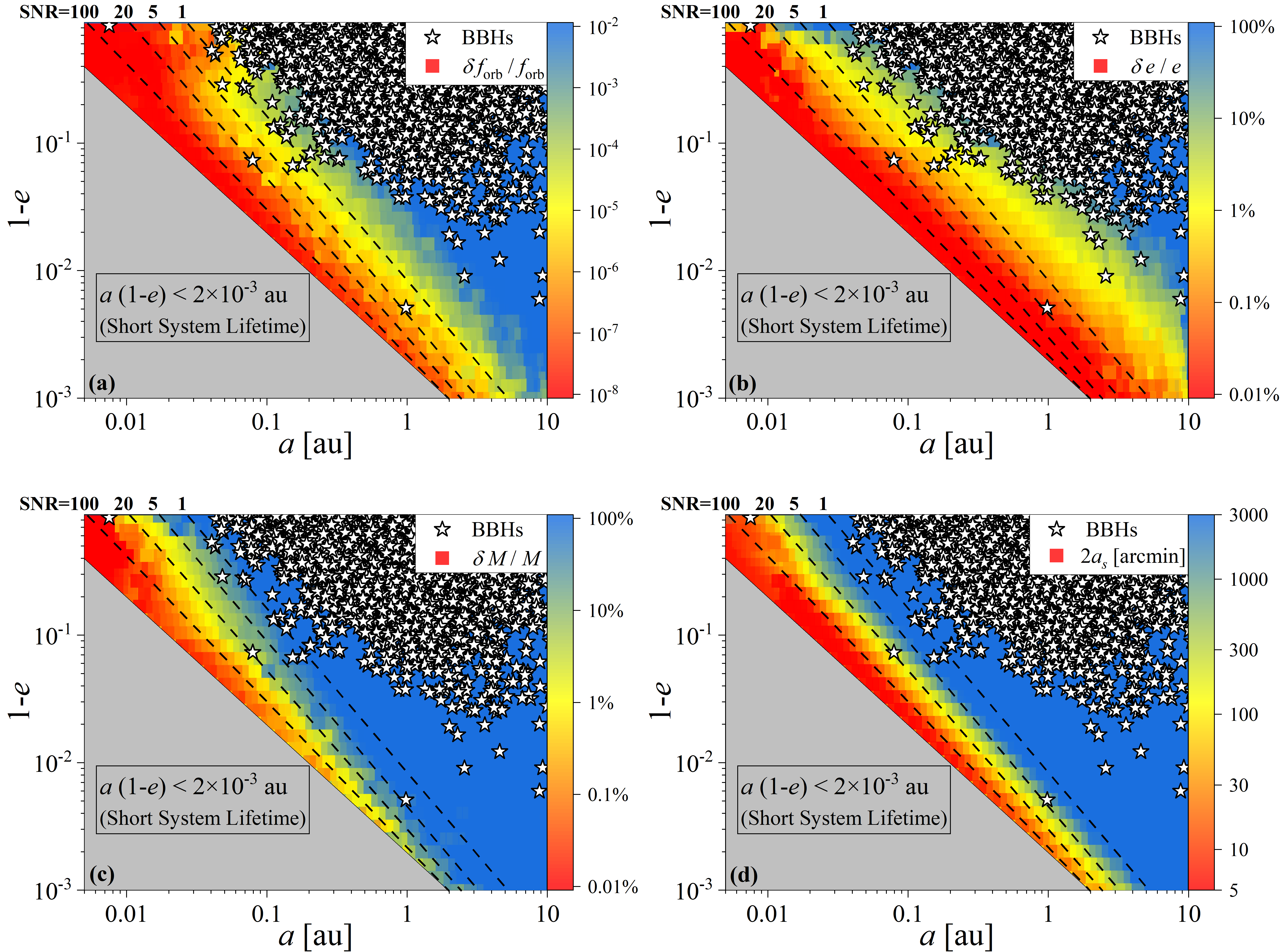
Figure 3: The population of BBHs from simulated Milky Way GCs, and their estimated parameter measurement error as a function of semi-major axis and eccentricity (for 5-yr observation). Here, we adopt the simulation result of the compact binary population in the Milky Way globular clusters (see Section 2, note that here we show a single realization of the in-cluster and ejected BBHs from Milky Way GCs), and plot the semi-major axis and eccentricity (as $1-e$) of each BBH system (see the white stars). The background color maps the compact binary’s parameter measurement error, for the orbital frequency ($\delta f_{\rm orb}/f_{\rm orb}$, Panel a), eccentricity ($\delta e/e$, Panel b), total mass ($\delta M/M$, Panel c), and sky location (major axis of sky error ellipsoid, $2a_{s}$, Panel d). We note that, in reality, the BBHs can have different mass, inclination, and sky locations, which affects their parameter measurement. However, for simplicity, here we assume a fixed intrinsic parameter of $m_{1}=10$ M${}_{\odot},$ $m_{2}=15$ M${}_{\odot},$ $R=8$ kpc and $\Phi=\Theta=\theta=\phi=\psi=\pi/4$ when estimating the Fisher matrix and mapping the parameter measurement accuracy. In each panel, the dashed lines represent equal signal-to-noise ratio contours (analytically calculated using Equation (2)), with $\rm SNR=1,\,5,\,20,\,100$ from right to left. We exclude the parameter space where the binary has a pericenter distance smaller than $a(1-e)<2\times 10^{-3}\,\rm au$, since they have a short merger timescale and negligible number expectation in our simulation.

Furthermore, we include the detector’s annual motion around the Sun to analyze the realistic detection of Milky Way BBHs (the detector response function, see, e.g., Cutler (1998); Cornish & Rubbo (2003); Kocsis et al. (2007) for more details). Consequently, the GW signal from an eccentric binary can be parameterized using:

$$h(t)=h(t;\boldsymbol{\lambda}=\left\{f_{\rm orb,0},1-e_{0},M,q,\cos\Theta,\Phi,\cos\theta,\phi,R,\psi\right\}),$$ (9)

in which $f_{\rm orb,0},e_{0}$ are the initial orbital frequency and eccentricity of the binary , $\Theta$ and $\Phi$ represent the spherical polar angles of the observer as viewed in the non-rotating, comoving frame of the compact object binary (i.e., the propagation direction of the GW signal viewed in the source’s frame); $\theta$ and $\phi$ are the spherical polar angles describing the sky location of the GW source viewed in the comoving frame of the solar system, where the LISA detector undergoes annual motion around the sun; $R$ is the binary’s distance from the detector (which is set as the distance of the GC hosting this binary), and $\psi$ is the polarization angle of the GW signal. For more details on the parameterization, see Sec. B in Xuan et al. (2024b).

After generating the GW signal as described by Equation (9), we compute the partial derivatives of the waveform with respect to each parameter (see Equation (7)). For example, to calculate $\partial h/\partial M$, we vary the total mass $M\rightarrow M^{\prime}=M+dM$, and generate a new waveform $h^{\prime}(t)=h^{\prime}(t;\boldsymbol{\lambda}^{\prime})$, where $\boldsymbol{\lambda}^{\prime}=\left\{f_{\rm orb},1-e,M+dM,q,\cos\Theta,\Phi,\cos\theta,\phi,R,\psi\right\}$. The partial derivative is then approximated as $\partial h/\partial M\approx[h^{\prime}(t)-h(t)]/\Delta M$. Note that each partial derivative is a time series representing the difference in the waveform caused by slightly varying one of the parameters around the central value. Also, in the numerical computation, we choose the parameter variation $d\lambda_{i}$ such that $\left\langle\left.dh\right\rvert\,dh\right\rangle\sim 10^{-3}\left\langle\left.h\right\rvert\,h\right\rangle$, ensuring the change in the waveform is small when computing the numerical derivative.

Finally, we compute the inner products between derivative waveforms using Equation (6), then substitute the results into Equation (7) to calculate $F_{ij}$. The parameter measurement errors are then estimated by inverting $F_{ij}$, as described in Equation (8)). We summarize the results in Figures 3 - 4 (note that Fisher matrix analysis yields the measurement error for all the parameters, $\left\{f_{\rm orb,0},1-e_{0},M,q,\cos\Theta,\Phi,\cos\theta,\phi,R,\psi\right\}$, but here we only show some of them to avoid clustering).

In Figure 3, we present a realistic example of the parameter measurement error for BBHs in Milky Way GCs. The white stars in the figure represent all the in-cluster and ejected BBHs from one realization of our simulated Milky Way GCs. In the background, we use different colors to show the parameter measurement errors, $\delta\lambda_{i}$, as a function of the BBHs’ orbital parameters, $(a,1-e)$. Particularly, Panel a shows the relative error in orbital frequency measurement, $\delta f_{\rm orb}/f_{\rm orb}$; Panel b shows the relative error in eccentricity measurement, $\delta e/e$; Panel c shows the relative error in total mass, $\delta M/M$; and Panel d shows the absolute error in sky location ($2a_{s}$, as the major axis of the sky error ellipsoids, see e.g., Lang & Hughes (2006); Kocsis et al. (2008, 2007); Mikóczi et al. (2012)). To ensure consistency in mapping the parameter measurement errors, we fix specific BBH parameters when computing the Fisher matrix results shown in Figure 3 ($m_{1}=10$ M${}_{\odot},$ $m_{2}=15$ M${}_{\odot},$ $R=8$ kpc and $\Phi=\Theta=\theta=\phi=\pi/4$, assuming a 5-year observation). However, BBHs in Milky Way GCs can have different mass, inclination, and sky locations, which potentially affects their parameter measurement . Therefore, the value shown by background colors in Figure 3 should be interpreted as heuristic estimates of the realistic accuracy.

We highlight that, the estimation shown in Figure 3 is agnostic to different BBH formation channels. In other words, for any potential BBH population in the galaxy, not necessarily from the GCs, their orbital parameter $(a,1-e)$ can be over-plotted on the figure to estimate the parameter measurement errors in a similar way. Moreover, Figure 3 indicates that our analysis of the parameter measurement accuracy is robust to variations in simulation results. For example, in Panels $a$ and $b$, regions with $\rm SNR>1$ (to the left of the dashed line at $\rm SNR=1$) show $\delta f_{\rm orb}/f_{\rm orb}\lesssim 10^{-5}$ and $\delta e/e\lesssim 10\%$. This suggests that, in realistic observations, BBH systems detected in the Milky Way GCs can typically achieve high accuracy measurements of $f_{\rm orb}$ and $e$. Furthermore, as shown by Panel c, BBHs with $\rm SNR>20$ can have a mass measurement accuracy of $\delta M/M\lesssim 10\%$. However, marginally detectable sources may have poorly constrained total mass (blue regions near the dashed line of $\rm SNR=5$). Similarly, Panel d shows that BBHs with $\rm SNR>20$ can have a sky localization accuracy of $2a_{s}\lesssim 300$ arcmins (yellow regions), which indicates that high-SNR BBHs can generally be localized with an angular resolution of a few degrees in the Milky Way.

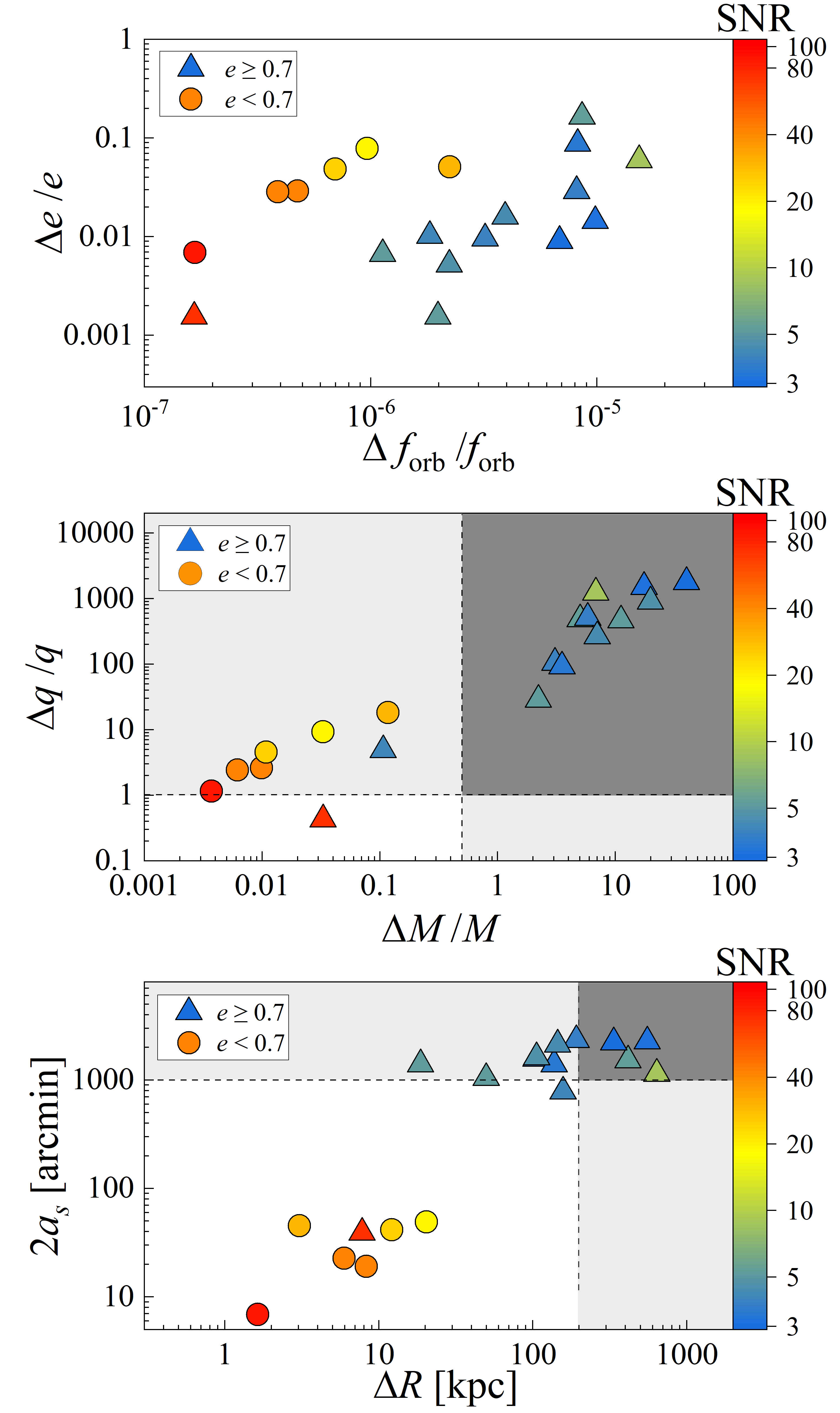
Figure 4: Parameter Measurement error of the detectable BBHs in simulated Milky Way GCs, estimated using Fisher matrix analysis. Here we adopt the simulation results of BBHs population in Milky Way GCs, with a total of 10 realizations. Each point in the figure represents a BBH system in the simulation, with the color showing the $\rm SNR$ of its GW signal (assuming a 5-year observation) and the shape showing the eccentricity of the orbit ($e>0.7$, plotted in triangles; $e<0.7$, plotted in circles). Upper Panel shows the relative error of orbital frequency and eccentricity measurement. Middle Panel shows the relative error of total mass and mass ratio measurement. In Bottom Panel, we show the absolute error of the BBHs’ distance measurement (x-axis), and their sky localization accuracy (as the major axis of the sky error ellipsoids, $2a_{s}$, on the y-axis). We exclude the parameter space where measurement accuracy is insufficient to help with the astrophysical interpretation, as marked using grey-shaded regions.

In Figure 4, we summarize all BBHs with $\rm SNR>3$ (assuming a 5-year observation) from the simulation and compute their exact parameter measurement errors. These BBHs are drawn from 10 realizations in total, excluding the ejected population due to the poor constraints on their location within the Milky Way. In particular, Upper Panel shows the relative errors in orbital frequency and eccentricity measurements; Middle Panel shows the relative error in total mass and mass ratio measurements; and Bottom Panel shows the absolute error in the distance (x-axis) and sky localization (y-axis) measurements. In each panel, we use different colors to show the SNR of BBHs and the shape of dots to show the eccentricity ($e>0.7$, plotted in triangles; $e<0.7$, plotted in circles). Additionally, we exclude the parameter space where measurement accuracy is insufficient for astrophysical interpretation, as marked using grey-shaded regions. Specifically, in the Middle Panel, regions with $\Delta M/M>50\%$ and $\Delta q/q>100\%$ are excluded, as the BBHs in these regions are indistinguishable from other compact binary sources, such as binary neutron stars (BNSs) or double white dwarfs (DWDs). Similarly, in the Bottom Panel, BBHs with $2a_{s}>1000$ arcmins ($\sim 5-10$ times the typical tidal radius of the Milky Way GCs) and $\Delta R>200$ kpc (halo radius of the Milky Way) cannot be confidently localized within a Milky Way globular cluster.

As shown in the Upper Panel, most detectable BBHs in Milky Way GCs have well-constrained orbital frequency and eccentricity. In particular, the fractional error in orbital frequency, $\delta f_{\rm orb}/f_{\rm orb}$, reaches an accuracy of $\sim 10^{-7}-10^{-5}$ for BBHs with $\rm SNR>3$, which indicates a frequency resolution of $\delta f_{\rm orb}\lesssim 10^{-10}$ Hz in LISA data analysis (see, e.g., Eq.18 in Xuan et al., 2024b, for an analytical explanation). Furthermore, all sources in Figure 4 have eccentricity measurement errors below $\delta e/e<1$, which allows us to confidently detect non-zero eccentricities and distinguish dynamically-formed BBHs from circular binaries created via isolated evolutionary channels. Additionally, highly eccentric sources typically exhibit higher accuracy in eccentricity measurement, with $\delta e/e$ reaching $\sim 0.1\%-10\%$ for BBHs with $e>0.7$. This trend is consistent with the results of our previous works (Xuan et al., 2023a), which shows that eccentricity can break the degeneracy of waveform and significantly enhance the parameter measurement. In general, accurate measurements of orbital frequency and eccentricity can provide valuable insights into the long-term evolution of BBHs, enable the detection of potential environmental effects, and help infer different formation channels.

Figure 5: Parameter Measurement error of an example BBH system in Milky Way Globular Clusters, estimated using Bayesian analysis. Here we consider the GW signal from a BBH system in the simulation, with intrinsic parameters of $m_{1}=23.3$ M${}_{\odot},$ $m_{2}=18.6$ M${}_{\odot},$ $a=0.06332$ au ($f_{\rm orb}=1.28771635\times 10^{-5}$ Hz), $e=0.897,$ $R=4.9$ kpc, assuming $\Phi=\Theta=\theta=\phi=\psi=\pi/4$ for simplicity. The color maps show the posterior distributions of the binary’s observed parameters (1-$\sigma$ to 5-$\sigma$ level, from red to blue), assuming a uniform a priori distribution and stationary Gaussian LISA noise. Note that this system has a SNR of $\sim 75$ for 5-year observation. For demonstration purposes, we use the cross in each panel to indicate the system’s intrinsic parameters. Furthermore, to avoid high computational cost, we do not include a full Bayesian analysis of all the 10 parameters, but only treat two of them as random variables in each panel (see the x and y axes) and fix the value of others.

On the other hand, mHz GW detection may be less sensitive to the mass of BBHs in the Milky Way, primarily due to degeneracies in the waveform . For example, most BBHs in the Middle Panel do not have a well-constrained mass ratio, with the relative error of measurement exceeding $\delta q/q\gtrsim 100\%$ (except for one highly eccentric BBH system with $\rm SNR\sim 75$, indicated by the red triangle in the bottom-left corner of Middle Panel). However, the total mass measurement is sufficiently accurate for a significant fraction of detectable BBHs, reaching $\delta M/M\sim 1\%-10\%$ for sources with $\rm SNR\gtrsim 20$ (see the red and orange dots to the left of the dashed line). Therefore, we expect LISA to accurately measure the mass of these high-SNR BBHs in the Milky Way GCs, making them distinguishable from BNSs and DWDs.

Furthermore, we highlight that, LISA can accurately localize most BBHs with $\rm SNR>20$ in Milky Way GCs (see the red and orange dots in Bottom Panel). In particular, these GW sources have a sky localization accuracy of $\sim 10-100$ arcmins (i.e., less than a few degrees), which is comparable to the typical tidal radius of Milky Way GCs ($\sim 100-200$ arcmins, see, e.g., Harris (2010)). As a result, LISA can localize BBH sources in specific Milky Way GCs, providing unique information about the Milky Way’s compact binary formation and the dynamical environment of GCs. Additionally, while the distance of BBHs is less precisely constrained compared to their sky location, most systems with $\rm SNR>20$ have a distance measurement error of $\Delta R\sim 1-100$ kpc in the Milky Way. Given the significant distance to the nearby galaxies (e.g., the Andromeda Galaxy is located at $\sim 780$ kpc), we expect these BBHs to be distinguishable from extragalactic GW sources.

We note that, although Fisher matrix analysis has been widely used to estimate the parameter measurement error for LISA sources, this method can sometimes yield inaccurate results, particularly for degenerate parameters or parameters with weak influences on the shape of GW signal (see, e.g., Vallisneri, 2008; Toubiana et al., 2020). Consequently, the parameter measurement accuracy presented in Figures  3 and 4 should be interpreted as a heuristic estimation, (especially for the mass parameters $M$ and $q$; see, e.g., Xuan et al., 2024b, for more details). Nevertheless, these estimates provide compelling evidence that BBHs in Milky Way GCs are promising targets for inferring their astrophysical properties.

To further validate the Fisher matrix results, we performed a Bayesian analysis (see, e.g., Finn, 1992; Cutler & Flanagan, 1994; Christensen & Meyer, 1998; Christensen et al., 2004), as shown in Figure 5. In particular, we choose an example BBH system from the simulation results (intrinsic parameters $m_{1}=23.3$ M${}_{\odot},$ $m_{2}=18.6$ M${}_{\odot},$ $a=0.06332$ au, $e=0.897,$ $R=4.9$ kpc), and inject its GW signal $s_{0}(t;\boldsymbol{\lambda})$ into a simulated stationary Gaussian LISA noise $n(t)$. We then vary the parameters slightly around their intrinsic values of $\boldsymbol{\lambda}$, generate different GW templates $s(t;\boldsymbol{\lambda}^{\prime})$, and compute their inner product with the mock signal $z(t)=s_{0}(t;\boldsymbol{\lambda})+n(t)$ (see Equation (6)). The posterior distribution of the example binary’s observed parameters is then computed using the aforementioned inner products $\langle s\mid z\rangle$, following equations 1-6 in Ref. Christensen et al. (2004). Due to the high computational cost, our comparison does not include a full Bayesian analysis of all the 10 parameters but only varies two of them in each panel (see the x and y axes) and fixes the others. We compute the results for five representative parameters, $f_{\rm orb}$, $e$, $M$, $R$, and $\phi$ (which is one of the sky location angles, representing the source’s sky localization accuracy).

As shown by Figure 5, despite the degeneracies and bias of some parameters, Bayesian analysis yields their measurement error (as indicated by the size of the 3-$\sigma$ level contours in Figure 4) comparable with the Fisher matrix estimation. Particularly, the Fisher matrix estimation of this example BBH system is represented by the red triangle to the bottom-left of each panel in Figure 4, with its parameter measurement error $\delta f_{\rm orb}\sim 2.1\times 10^{-12}$ Hz, $\delta e\sim 1.4\times 10^{-3},$ $\delta M\sim 1.4$ M${}_{\odot},$ $\delta R\sim 7.8$ kpc, and sky localization accuracy $2a_{s}\sim 39$ arcmin$\sim 0.65$ degrees. These values are consistent with the size of 3-$\sigma$ contours in Bayesian analysis (within one order of magnitude, see Figure 5), which partly justifies the Fisher matrix results of Figures 3 and 4.

4 Discussion

In this work, we explore the realistic detectability and parameter measurement accuracy of BBHs in Galactic GCs for observations with LISA. Particularly, since GCs are considered ideal environments for the dynamical formation of BBHs (see, e.g., Miller & Hamilton, 2002; Rodriguez et al., 2015; Samsing, 2018), constraining their detectability potential is of prime importance for the community. Notably, Kremer et al. (2018a) predicted that LISA might detect a significant number of BBH sources from $\sim 150$ GCs in the Milky Way, with various orbital parameters. Furthermore, many dynamically-formed BBHs can undergo a wide ($a\gtrsim 0.1\,\rm au$), highly eccentric ($e\gtrsim 0.9$) progenitor phase before merger (Kocsis & Levin, 2012; Hoang et al., 2019; Xuan et al., 2023b, 2024a, 2024b; Knee et al., 2024), which has been recently proposed to have unique imprints on the mHz GW detection. By detecting these eccentric sources, we can distinguish between different formation mechanisms (East et al., 2013; Samsing et al., 2014; Coughlin et al., 2015; Breivik et al., 2016; Vitale, 2016; Nishizawa et al., 2017; Zevin et al., 2017; Gondán et al., 2018a, b; Lower et al., 2018; Romero-Shaw et al., 2019; Moore et al., 2019; Abbott et al., 2021; The LIGO Scientific Collaboration et al., 2021; Zevin et al., 2021), enhance the parameter measurement accuracy (such as the orbital frequency evolution and source location, see Xuan et al., 2023a, 2024b), and probe the potential presence of tertiary companions through eccentricity oscillations (Thompson, 2011; Antognini et al., 2014; Hoang et al., 2018; Stephan et al., 2019; Martinez et al., 2020; Hoang et al., 2020; Naoz et al., 2020; Stephan et al., 2019; Wang et al., 2021; Knee et al., 2022).

Using CMC Cluster Catalog of Kremer et al. (2020) we generate a best-fit model for each Milky Way globular cluster , and estimate the BBH population within these clusters (illustrated in Figure 1). We then generate the BBHs’ GW signals using the x-model (Hinder et al., 2010), which incorporates the dynamics of eccentric compact binaries up to 3PN order. Additionally, the waveform analysis includes the detector’s annual motion around the Sun so that our results can represent the realistic detection of GW signals. More details of the waveform model and analysis method can be found in Xuan et al. (2024b).

Based on the simulation, we compute the number of detectable BBHs formed in Galactic GCs (see Section 3.1). In total, we expect the GW signal from $0.7\pm 0.7$, $2.0\pm 1.7$, $3.6\pm 2.3$, $13.4\pm 4.7$ BBHs to exceed the threshold of $\rm SNR=30$, 5, 3, and 1, respectively, for a 10-year observation of LISA. Among all these sources, in-cluster BBHs contribute to 0.7, 1.5, 2.2, and 5.8 GW sources, and the ejected population contributes to $\sim 0$, 0.5, 1.4, and 7.6 GW sources above the threshold of $\rm SNR=30$, 5, 3, 1. We highlight that $\sim 50\%$ of the BBHs with $\rm SNR>5$ has high eccentricity in the detection ($e\gtrsim 0.9$), which reflects the dominant population of eccentric BBHs in GCs (as they are long-living sources, see, e,g., Equation (4)), and indicates that most of the GW signals from BBHs in Milky Way GCs are characterized by highly eccentric “GW bursts” in future LISA detection (see, e.g., Xuan et al., 2023b).

Furthermore, we analyze the properties of Galactic GCs that are most likely to host resolvable LISA sources (see Figure 2). Specifically, we calculate the expected probability for a cluster to host a BBH system with $\rm SNR>1$ during a 10-year LISA observation. As shown in Figure 2, these BBH-hosting GCs tend to cluster within specific regions of the parameter space, where the GCs have a close distance to the detector ($R\lesssim 10$ kpc), exhibit a small $r_{c}/r_{h}$ ($\sim 0.1-0.3$), and have a large total mass.

To evaluate the measurement accuracy achievable with LISA, we performed a Fisher matrix analysis on the simulated BBH population, as illustrated in Figures 3 and 4. Particularly, Figure 3 maps the intrinsic parameters, $(a,1-e)$, of the simulated Milky Way GC BBH population and uses the background color to show their different parameter measurement errors (5-year observation); Figure 4 depicts the measurement error of $\{f_{\rm orb},e,M,q,R,2a_{s}\}$ for all the simulated BBHs with $\rm SNR>3$, across all the 10 realizations, for 5-year observation. As illustrated in both figures, most of the BBHs with $\rm SNR>3$ have well-constrained orbital frequency and eccentricity, reaching $\delta f_{\rm orb}/f_{\rm orb}\sim 10^{-7}-10^{-5}$ and $\delta e/e<1$. Furthermore, eccentricity can, in general, enhance the measurement accuracy, with $\delta e/e$ reaching $\sim 10^{-3}-0.1$ for detectable BBHs with $e>0.7$. On the other hand, BBHs with $\rm SNR>20$ can have a total mass measurement accuracy of $\delta M/M\lesssim 10\%$, but most of the marginally detectable sources may not have a well-constrained total mass and mass ratio. Also, we expect BBHs with $\rm SNR>20$ to be confidently localized with an angular resolution of $\sim 10-100$ arcmins, which enables us to localize these sources in specific Milky Way GCs. We further verified the Fisher matrix results against Bayesian analysis for an example system, as shown in Figure 5.

Although our collective sample of GC simulations effectively spans the full parameter space of Galactic GCs (Kremer et al., 2020), this simulation suite is a grid, which inevitably means some specific observed GCs do not necessarily have a strong “one-to-one” model match. For example, Ref. Rui et al. (2021), demonstrated how the CMC Catalog may be augmented with additional models to match particular GCs with observed properties lying in between grid points. In another recent study, Ye et al. (2022) showed that especially massive GCs like 47 Tuc (NGC 104) may require additional adjustments (in particular variations to the initial density profile and initial stellar mass function) to produce a precise model match. The ideal solution is to produce a separate model for every single Galactic cluster (for some examples, see Kremer et al., 2018b, 2019a; Ye et al., 2022, 2024); however, this is computationally expensive, and outside the scope of the current study. We tested the LISA predictions from our best-fit model for NGC 104 with the predictions from the more precise model in Ye et al. (2022), and found that the number of LISA sources is consistent within a factor of $3$ for SNR$>1$.

Additionally, this work simulates the BBH population in observed GCs of the Milky Way, which does not include other potential GW sources in the local galaxy, such as BBHs formed in the Galactic nucleus, Galactic Field, and evaporated GCs. Thus, the number expectation presented here only serves as a lower bound for the LISA detection. Notably, the high computational cost of $N-$body simulation limits the sample size presented in this paper (in total 10 realizations), which may result in uncertainty of the predicted BBH population. However, the prediction of source number and parameter measurement accuracy in this work is expected to be a realistic estimation, based on one of the most up-to-date simulations of GCs (Kremer et al., 2020). Also, the population properties presented here agree with previous works with different GC models (see, e.g., Kremer et al., 2018a), which indicates the robustness of the result that LISA can detect a handful of BBHs formed in the Milky Way GCs.

To conclude, mHz-frequency BBHs in Milky Way GCs have the potential to enable direct test of the role of GCs in the formation of GW sources. Given a 5-10 year LISA observation, these systems typically have highly-resolved orbital frequency ($\delta f_{\rm orb}/f_{\rm orb}\sim 10^{-7}-10^{-5}$) and eccentricity ($\delta e/e\sim 10^{-3}-0.1$), as well as a measurable total mass when the signal-to-noise ratio exceeds $\sim 20$. Furthermore, these high SNR BBHs can be confidently localized in a specific GC of the Milky Way, with an angular resolution of $\sim 10-100$ arcmins in the sky. Therefore, we highlight the potential of detecting BBHs in Milky Way GCs, which allows for accurate tracking of their long-term orbital evolution, distinguishing the compact binary formation mechanisms, and understanding the properties of GCs in the local galaxy.

References

- Aarseth (2012) Aarseth, S. J. 2012, MNRAS, 422, 841
- Abbott et al. (2021) Abbott, R., et al. 2021, ApJ, 913, L7
- Abbott et al. (2023) Abbott, R., Abbott, T. D., Acernese, F., et al. 2023, Phys. Rev. X, 13, 041039. https://link.aps.org/doi/10.1103/PhysRevX.13.041039
- Amaro-Seoane et al. (2017) Amaro-Seoane, P., et al. 2017, arXiv e-prints, arXiv:1702.00786
- Amaro-Seoane et al. (2022) —. 2022, arXiv e-prints, arXiv:2203.06016
- Antognini et al. (2014) Antognini, J. M., Shappee, B. J., Thompson, T. A., & Amaro-Seoane, P. 2014, MNRAS, 439, 1079
- Antonini & Gieles (2020) Antonini, F., & Gieles, M. 2020, MNRAS, 492, 2936
- Antonini & Gieles (2020) Antonini, F., & Gieles, M. 2020, Physical Review D, 102, doi:10.1103/physrevd.102.123016. https://doi.org/10.1103%2Fphysrevd.102.123016
- Arca Sedda et al. (2023) Arca Sedda, M., Naoz, S., & Kocsis, B. 2023, Universe, 9, 138
- Arca Sedda et al. (2018) Arca Sedda, M., Askar, A., & Giersz, M. 2018, Monthly Notices of the Royal Astronomical Society, 479, 4652. https://doi.org/10.1093/mnras/sty1859
- Barack & Cutler (2004) Barack, L., & Cutler, C. 2004, Phys. Rev. D, 69, 082005
- Baumgardt & Hilker (2018) Baumgardt, H., & Hilker, M. 2018, MNRAS, 478, 1520
- Belczynski et al. (2016) Belczynski, K., Holz, D. E., Bulik, T., & O’Shaughnessy, R. 2016, Nature, 534, 512
- Bird et al. (2016) Bird, S., Cholis, I., Muñoz, J. B., et al. 2016, Physical Review Letters, 116, doi:10.1103/physrevlett.116.201301. http://dx.doi.org/10.1103/PhysRevLett.116.201301
- Breen & Heggie (2013) Breen, P. G., & Heggie, D. C. 2013, Monthly Notices of the Royal Astronomical Society, 432, 2779. https://doi.org/10.1093/mnras/stt628
- Breivik et al. (2020) Breivik, K., Mingarelli, C. M. F., & Larson, S. L. 2020, ApJ, 901, 4
- Breivik et al. (2016) Breivik, K., Rodriguez, C. L., Larson, S. L., Kalogera, V., & Rasio, F. A. 2016, ApJ, 830, L18
- Brown & Zimmerman (2010) Brown, D. A., & Zimmerman, P. J. 2010, Phys. Rev. D, 81, 024007
- Chen et al. (2019) Chen, X., Li, S., & Cao, Z. 2019, MNRAS, 485, L141
- Christensen et al. (2004) Christensen, N., Dupuis, R. J., Woan, G., & Meyer, R. 2004, Phys. Rev. D, 70, 022001. https://link.aps.org/doi/10.1103/PhysRevD.70.022001
- Christensen & Meyer (1998) Christensen, N., & Meyer, R. 1998, Phys. Rev. D, 58, 082001. https://link.aps.org/doi/10.1103/PhysRevD.58.082001
- Chua et al. (2021) Chua, A. J. K., Katz, M. L., Warburton, N., & Hughes, S. A. 2021, Phys. Rev. Lett., 126, 051102
- Coe (2009) Coe, D. 2009, arXiv e-prints, arXiv:0906.4123
- Cornish & Rubbo (2003) Cornish, N. J., & Rubbo, L. J. 2003, Phys. Rev. D, 67, 022001. https://link.aps.org/doi/10.1103/PhysRevD.67.022001
- Coughlin et al. (2015) Coughlin, M., Meyers, P., Thrane, E., Luo, J., & Christensen, N. 2015, Physical Review D, 91, doi:10.1103/physrevd.91.063004. https://doi.org/10.1103%2Fphysrevd.91.063004
- Cutler (1998) Cutler, C. 1998, Phys. Rev. D, 57, 7089
- Cutler & Flanagan (1994) Cutler, C., & Flanagan, É. E. 1994, Phys. Rev. D, 49, 2658
- D’Orazio & Samsing (2018) D’Orazio, D. J., & Samsing, J. 2018, MNRAS, 481, 4775
- Downing et al. (2010) Downing, J. M. B., Benacquista, M. J., Giersz, M., & Spurzem, R. 2010, MNRAS, 407, 1946
- East et al. (2013) East, W. E., McWilliams, S. T., Levin, J., & Pretorius, F. 2013, Phys. Rev. D, 87, 043004
- Eldridge et al. (2019) Eldridge, J. J., Stanway, E. R., & Tang, P. N. 2019, MNRAS, 482, 870
- Fang et al. (2019) Fang, Y., Chen, X., & Huang, Q.-G. 2019, ApJ, 887, 210
- Finn (1992) Finn, L. S. 1992, Phys. Rev. D, 46, 5236
- Fragione & Bromberg (2019) Fragione, G., & Bromberg, O. 2019, MNRAS, 488, 4370
- Gautham Bhaskar et al. (2023) Gautham Bhaskar, H., Li, G., & Lin, D. 2023, arXiv e-prints, arXiv:2303.12539
- Gerosa et al. (2019) Gerosa, D., Ma, S., Wong, K. W. K., et al. 2019, arXiv e-prints, arXiv:1902.00021
- Gondán et al. (2018a) Gondán, L., Kocsis, B., Raffai, P., & Frei, Z. 2018a, The Astrophysical Journal, 860, 5. https://dx.doi.org/10.3847/1538-4357/aabfee
- Gondán et al. (2018b) —. 2018b, The Astrophysical Journal, 855, 34. https://dx.doi.org/10.3847/1538-4357/aaad0e
- Harris (1996) Harris, W. E. 1996, AJ, 112, 1487
- Harris (2010) —. 2010, arXiv e-prints, arXiv:1012.3224
- Heggie (2001) Heggie, D. C. 2001, The Gravitational Million-Body Problem, , , arXiv:astro-ph/0111045. https://arxiv.org/abs/astro-ph/0111045
- Hinder et al. (2010) Hinder, I., Herrmann, F., Laguna, P., & Shoemaker, D. 2010, Phys. Rev. D, 82, 024033
- Hoang et al. (2019) Hoang, B.-M., Naoz, S., Kocsis, B., Farr, W. M., & McIver, J. 2019, ApJ, 875, L31
- Hoang et al. (2018) Hoang, B.-M., Naoz, S., Kocsis, B., Rasio, F. A., & Dosopoulou, F. 2018, ApJ, 856, 140
- Hoang et al. (2020) Hoang, B.-M., Naoz, S., & Kremer, K. 2020, ApJ, 903, 8
- Huerta et al. (2014) Huerta, E. A., Kumar, P., McWilliams, S. T., O’Shaughnessy, R., & Yunes, N. 2014, Phys. Rev. D, 90, 084016
- Hughes et al. (2021) Hughes, S. A., Warburton, N., Khanna, G., Chua, A. J. K., & Katz, M. L. 2021, Phys. Rev. D, 103, 104014
- Katz et al. (2021) Katz, M. L., Chua, A. J. K., Speri, L., Warburton, N., & Hughes, S. A. 2021, Phys. Rev. D, 104, 064047
- Klein et al. (2016) Klein, A., Barausse, E., Sesana, A., et al. 2016, Phys. Rev. D, 93, 024003
- Knee et al. (2024) Knee, A. M., McIver, J., Naoz, S., Romero-Shaw, I. M., & Hoang, B.-M. 2024, Detecting gravitational-wave bursts from black hole binaries in the Galactic Center with LISA, , , arXiv:2404.12571. https://arxiv.org/abs/2404.12571
- Knee et al. (2022) Knee, A. M., Romero-Shaw, I. M., Lasky, P. D., McIver, J., & Thrane, E. 2022, ApJ, 936, 172
- Kocsis et al. (2008) Kocsis, B., Haiman, Z., & Menou, K. 2008, The Astrophysical Journal, 684, 870–887. http://dx.doi.org/10.1086/590230
- Kocsis et al. (2007) Kocsis, B., Haiman, Z., Menou, K., & Frei, Z. 2007, Phys. Rev. D, 76, 022003
- Kocsis & Levin (2012) Kocsis, B., & Levin, J. 2012, Physical Review D, 85, doi:10.1103/physrevd.85.123005. https://doi.org/10.1103%2Fphysrevd.85.123005
- Kocsis & Levin (2012) Kocsis, B., & Levin, J. 2012, Phys. Rev. D, 85, 123005
- Kremer et al. (2018a) Kremer, K., Chatterjee, S., Breivik, K., et al. 2018a, Phys. Rev. Lett., 120, 191103
- Kremer et al. (2019a) Kremer, K., Chatterjee, S., Ye, C. S., Rodriguez, C. L., & Rasio, F. A. 2019a, ApJ, 871, 38
- Kremer et al. (2021) Kremer, K., Rui, N. Z., Weatherford, N. C., et al. 2021, ApJ, 917, 28
- Kremer et al. (2018b) Kremer, K., Ye, C. S., Chatterjee, S., Rodriguez, C. L., & Rasio, F. A. 2018b, ApJ, 855, L15
- Kremer et al. (2019b) Kremer, K., Rodriguez, C. L., Amaro-Seoane, P., et al. 2019b, Phys. Rev. D, 99, 063003
- Kremer et al. (2020) Kremer, K., Ye, C. S., Rui, N. Z., et al. 2020, The Astrophysical Journal Supplement Series, 247, 48. https://dx.doi.org/10.3847/1538-4365/ab7919
- Kroupa (2001) Kroupa, P. 2001, MNRAS, 322, 231
- Kulkarni et al. (1993) Kulkarni, S. R., Hut, P., & McMillan, S. 1993, Nature, 364, 421
- Lamberts et al. (2018) Lamberts, A., Garrison-Kimmel, S., Hopkins, P. F., et al. 2018, MNRAS, 480, 2704
- Lang & Hughes (2006) Lang, R. N., & Hughes, S. A. 2006, Phys. Rev. D, 74, 122001. https://link.aps.org/doi/10.1103/PhysRevD.74.122001
- Lower et al. (2018) Lower, M. E., Thrane, E., Lasky, P. D., & Smith, R. 2018, Phys. Rev. D, 98, 083028. https://link.aps.org/doi/10.1103/PhysRevD.98.083028
- Mackey et al. (2007) Mackey, A. D., Wilkinson, M. I., Davies, M. B., & Gilmore, G. F. 2007, MNRAS, 379, L40
- Martinez et al. (2020) Martinez, M. A. S., Fragione, G., Kremer, K., et al. 2020, ApJ, 903, 67
- Merritt et al. (2004) Merritt, D., Piatek, S., Portegies Zwart, S., & Hemsendorf, M. 2004, ApJ, 608, L25
- Michaely & Naoz (2022) Michaely, E., & Naoz, S. 2022, ApJ, 936, 184
- Michaely & Perets (2019) Michaely, E., & Perets, H. B. 2019, ApJ, 887, L36
- Michaely & Perets (2020) —. 2020, MNRAS, 498, 4924
- Mikóczi et al. (2012) Mikóczi, B., Kocsis, B., Forgács, P., & Vasúth, M. 2012, Phys. Rev. D, 86, 104027
- Miller & Hamilton (2002) Miller, M. C., & Hamilton, D. P. 2002, ApJ, 576, 894
- Moore et al. (2019) Moore, C. J., Gerosa, D., & Klein, A. 2019, MNRAS, 488, L94
- Morscher et al. (2015) Morscher, M., Pattabiraman, B., Rodriguez, C., Rasio, F. A., & Umbreit, S. 2015, ApJ, 800, 9
- Muñoz et al. (2022) Muñoz, D. J., Stone, N. C., Petrovich, C., & Rasio, F. A. 2022, arXiv e-prints, arXiv:2204.06002
- Naoz (2016) Naoz, S. 2016, ARA&A, 54, 441
- Naoz & Haiman (2023) Naoz, S., & Haiman, Z. 2023, arXiv e-prints, arXiv:2307.11149
- Naoz et al. (2022) Naoz, S., Rose, S. C., Michaely, E., et al. 2022, ApJ, 927, L18
- Naoz et al. (2020) Naoz, S., Will, C. M., Ramirez-Ruiz, E., et al. 2020, ApJ, 888, L8
- Nishizawa et al. (2017) Nishizawa, A., Sesana, A., Berti, E., & Klein, A. 2017, MNRAS, 465, 4375
- O’Leary et al. (2009) O’Leary, R. M., Kocsis, B., & Loeb, A. 2009, MNRAS, 395, 2127
- Peng & Chen (2021) Peng, P., & Chen, X. 2021, MNRAS, 505, 1324
- Peters & Mathews (1963) Peters, P. C., & Mathews, J. 1963, Physical Review, 131, 435
- Peuten et al. (2016) Peuten, M., Zocchi, A., Gieles, M., Gualandris, A., & Hénault-Brunet, V. 2016, MNRAS, 462, 2333
- Portegies Zwart & McMillan (2002) Portegies Zwart, S. F., & McMillan, S. L. W. 2002, ApJ, 576, 899
- Robson et al. (2019) Robson, T., Cornish, N. J., & Liu, C. 2019, Classical and Quantum Gravity, 36, 105011
- Robson et al. (2018) Robson, T., Cornish, N. J., Tamanini, N., & Toonen, S. 2018, Phys. Rev. D, 98, 064012
- Rodriguez et al. (2018) Rodriguez, C. L., Amaro-Seoane, P., Chatterjee, S., et al. 2018, Phys. Rev. D, 98, 123005
- Rodriguez et al. (2016a) Rodriguez, C. L., Chatterjee, S., & Rasio, F. A. 2016a, Phys. Rev. D, 93, 084029
- Rodriguez et al. (2016b) Rodriguez, C. L., Haster, C.-J., Chatterjee, S., Kalogera, V., & Rasio, F. A. 2016b, ApJ, 824, L8
- Rodriguez et al. (2015) Rodriguez, C. L., Morscher, M., Pattabiraman, B., et al. 2015, Physical Review Letters, 115, 051101
- Rodriguez et al. (2022) Rodriguez, C. L., Weatherford, N. C., Coughlin, S. C., et al. 2022, ApJS, 258, 22
- Rom et al. (2024) Rom, B., Linial, I., Kaur, K., & Sari, R. 2024, Dynamics around supermassive black holes: Extreme mass-ratio inspirals as gravitational-wave sources, , , arXiv:2406.19443. https://arxiv.org/abs/2406.19443
- Romero-Shaw et al. (2019) Romero-Shaw, I. M., Lasky, P. D., & Thrane, E. 2019, Monthly Notices of the Royal Astronomical Society, 490, 5210–5216. http://dx.doi.org/10.1093/mnras/stz2996
- Rui et al. (2021) Rui, N. Z., Kremer, K., Weatherford, N. C., et al. 2021, ApJ, 912, 102
- Samsing (2018) Samsing, J. 2018, Phys. Rev. D, 97, 103014
- Samsing & D’Orazio (2019) Samsing, J., & D’Orazio, D. J. 2019, Phys. Rev. D, 99, 063006
- Samsing et al. (2019) Samsing, J., Hamers, A. S., & Tyles, J. G. 2019, Phys. Rev. D, 100, 043010
- Samsing et al. (2014) Samsing, J., MacLeod, M., & Ramirez-Ruiz, E. 2014, ApJ, 784, 71
- Samsing et al. (2022) Samsing, J., Bartos, I., D’Orazio, D. J., et al. 2022, Nature, 603, 237
- Sasaki et al. (2016) Sasaki, M., Suyama, T., Tanaka, T., & Yokoyama, S. 2016, Physical Review Letters, 117, doi:10.1103/physrevlett.117.061101. http://dx.doi.org/10.1103/PhysRevLett.117.061101
- Sesana et al. (2020) Sesana, A., Lamberts, A., & Petiteau, A. 2020, Mon. Not. Roy. Astron. Soc., 494, L75
- Sigurdsson & Hernquist (1993) Sigurdsson, S., & Hernquist, L. 1993, Nature, 364, 423
- Spitzer (1969) Spitzer, Lyman, J. 1969, ApJ, 158, L139
- Stegmann et al. (2024) Stegmann, J., Vigna-Gómez, A., Rantala, A., et al. 2024, The Astrophysical Journal Letters, 972, L19. http://dx.doi.org/10.3847/2041-8213/ad70bb
- Stephan et al. (2019) Stephan, A. P., Naoz, S., Ghez, A. M., et al. 2019, ApJ, 878, 58
- Stevenson et al. (2017) Stevenson, S., Vigna-Gómez, A., Mandel, I., et al. 2017, Nature Communications, 8, doi:10.1038/ncomms14906. http://dx.doi.org/10.1038/ncomms14906
- Tagawa et al. (2021) Tagawa, H., Kocsis, B., Haiman, Z., et al. 2021, ApJ, 907, L20
- Tamanini et al. (2020) Tamanini, N., Klein, A., Bonvin, C., Barausse, E., & Caprini, C. 2020, Phys. Rev. D, 101, 063002
- Tang et al. (2024) Tang, P., Eldridge, J. J., Meyer, R., et al. 2024, MNRAS, 534, 1707
- The LIGO Scientific Collaboration et al. (2021) The LIGO Scientific Collaboration, the Virgo Collaboration, the KAGRA Collaboration, et al. 2021, arXiv e-prints, arXiv:2111.03634
- Thompson (2011) Thompson, T. A. 2011, ApJ, 741, 82
- Torres-Orjuela et al. (2021) Torres-Orjuela, A., Amaro Seoane, P., Xuan, Z., et al. 2021, Phys. Rev. Lett., 127, 041102
- Toubiana et al. (2020) Toubiana, A., Marsat, S., Babak, S., Barausse, E., & Baker, J. 2020, Physical Review D, 101, doi:10.1103/physrevd.101.104038. http://dx.doi.org/10.1103/PhysRevD.101.104038
- Vallisneri (2008) Vallisneri, M. 2008, Physical Review D, 77, doi:10.1103/physrevd.77.042001. http://dx.doi.org/10.1103/PhysRevD.77.042001
- Vitale (2016) Vitale, S. 2016, Physical Review Letters, 117, 051102
- Vitale (2021) Vitale, S. 2021, Science, 372, eabc7397. https://www.science.org/doi/abs/10.1126/science.abc7397
- Vitale & Whittle (2018) Vitale, S., & Whittle, C. 2018, Physical Review D, 98, doi:10.1103/physrevd.98.024029. http://dx.doi.org/10.1103/PhysRevD.98.024029
- Wagg et al. (2022) Wagg, T., Broekgaarden, F. S., de Mink, S. E., et al. 2022, ApJ, 937, 118
- Wang et al. (2021) Wang, H., Stephan, A. P., Naoz, S., Hoang, B.-M., & Breivik, K. 2021, ApJ, 917, 76
- Wang et al. (2016) Wang, L., Spurzem, R., Aarseth, S., et al. 2016, MNRAS, 458, 1450
- Wen (2003) Wen, L. 2003, ApJ, 598, 419
- Winter-Granić et al. (2023) Winter-Granić, M., Petrovich, C., & Peña-Donaire, V. 2023, Binary mergers in the centers of galaxies: synergy between stellar flybys and tidal fields, , , arXiv:2312.17319
- Xuan et al. (2023a) Xuan, Z., Naoz, S., & Chen, X. 2023a, Phys. Rev. D, 107, 043009
- Xuan et al. (2023b) Xuan, Z., Naoz, S., Kocsis, B., & Michaely, E. 2023b, arXiv e-prints, arXiv:2310.00042
- Xuan et al. (2024a) Xuan, Z., Naoz, S., Kocsis, B., & Michaely, E. 2024a, Phys. Rev. D, 110, 023020. https://link.aps.org/doi/10.1103/PhysRevD.110.023020
- Xuan et al. (2021) Xuan, Z., Peng, P., & Chen, X. 2021, MNRAS, 502, 4199
- Xuan et al. (2024b) Xuan, Z., Naoz, S., Li, A. K. Y., et al. 2024b, arXiv e-prints, arXiv:2409.15413
- Ye et al. (2019) Ye, C. S., Kremer, K., Chatterjee, S., Rodriguez, C. L., & Rasio, F. A. 2019, ApJ, 877, 122
- Ye et al. (2024) Ye, C. S., Kremer, K., Ransom, S. M., & Rasio, F. A. 2024, ApJ, 975, 77
- Ye et al. (2022) Ye, C. S., Kremer, K., Rodriguez, C. L., et al. 2022, ApJ, 931, 84
- Zevin et al. (2017) Zevin, M., Pankow, C., Rodriguez, C. L., et al. 2017, ApJ, 846, 82
- Zevin et al. (2021) Zevin, M., Romero-Shaw, I. M., Kremer, K., Thrane, E., & Lasky, P. D. 2021, The Astrophysical Journal Letters, 921, L43. https://dx.doi.org/10.3847/2041-8213/ac32dc
- Zevin et al. (2019) Zevin, M., Samsing, J., Rodriguez, C., Haster, C.-J., & Ramirez-Ruiz, E. 2019, The Astrophysical Journal, 871, 91. https://dx.doi.org/10.3847/1538-4357/aaf6ec
- Zhang et al. (2021) Zhang, F., Chen, X., Shao, L., & Inayoshi, K. 2021, ApJ, 923, 139
- Zhang & Chen (2024) Zhang, Z., & Chen, X. 2024, arXiv e-prints, arXiv:2402.02178
- Zocchi et al. (2019) Zocchi, A., Gieles, M., & Hénault-Brunet, V. 2019, MNRAS, 482, 4713