Bridging Entanglement and Magic Resources through Operator Space

Abstract

Local operator entanglement (LOE) dictates the complexity of simulating Heisenberg evolution using tensor network methods, and serves as strong dynamical signature of quantum chaos. We show that LOE is also sensitive to how non-Clifford a unitary is: its magic resources. In particular, we prove that LOE is always upper-bound by three distinct magic monotones: $T$-count, unitary nullity, and operator stabilizer Rényi entropy. Moreover, in the average case for large, random circuits, LOE and magic monotones approximately coincide. Our results imply that an operator evolution that is expensive to simulate using tensor network methods must also be inefficient using both stabilizer and Pauli truncation methods. A direct corollary of our bounds is that any quantum chaotic dynamics cannot be simulated classically. Entanglement in operator space therefore measures a unified picture of non-classical resources, in stark contrast to the Schrödinger picture.

Introduction.— The growth of non-classical resources in quantum dynamics indicates a necessary piece of the puzzle separating classical and quantum simulability. Understanding this separation is essential to a complete characterization of such systems, both from an algorithmic and from a physical perspective. Arguably the most famous of these resources is entanglement: it both governs the efficiency of tensor network methods Verstraete and Cirac (2006); Schuch et al. (2008), and witnessing quantum critical phase transitions Vidal et al. (2003); Calabrese and Cardy (2004); Hastings (2007); Eisert et al. (2010); Silvi et al. (2010). Similarly, the concept of non-stabilizerness—or magic—has emerged as another key resource of non-classicality. It is well-known that Clifford dynamics can be simulated efficiently on a classical computer by tracking the $N$ stabilizer generators of an $N$-qubit state Gottesman (1998); Aaronson and Gottesman (2004). Including a $T$-gate in the gateset is all that is required to remove these generators and achieve universality—and indeed the best known Clifford+$T$ simulators scale exponentially in the number of $T$-gates Pashayan et al. (2022); Bravyi et al. (2019). This departure from stabilizerness can be formalized rigorously in the theory of magic, where $T$-count forms just one example aspect Howard and Campbell (2017); Beverland et al. (2020); Leone et al. (2022); Liu and Winter (2022). Recently, magic resources have also been found to play a key role in phase transitions White et al. (2021); Niroula et al. (2024); Catalano et al. (2024); Fux et al. (2024a), dynamical complexity Leone et al. (2022); Garcia et al. (2023); Oliviero et al. (2024); Gu et al. (2024); Ahmadi and Greplova (2024); Odavic et al. (2024a), and (pseudo-)randomness Haferkamp et al. (2022a); Leone et al. (2021).

Given the clear role each of these concepts individually play in both quantum information theory and many-body physics, one would hope to transitively understand the direct connection between the two. A question of foundational importance is therefore: How are the two disparate resources of magic and entanglement related to one other? The solution is not a priori obvious, at least in the usual quantum state setting. For instance, entanglement tends to grow maximally in Clifford circuits. On the other hand, product states can have high magic resource. And although details of the entanglement spectrum Chamon et al. (2014) can serve as witness to magic in a state Tirrito et al. (2024a); Turkeshi et al. (2023), even a single $T$-gate can make this spectrum consistent with random matrix theory predictions Zhou et al. (2020). Even more puzzlingly, there appears no clear connection to the integrability of the underlying dynamics in a many-body setting. Locally-interacting integrable and chaotic models alike produce linearly growing entanglement after a quench Calabrese and Cardy (2005); Chiara et al. (2006); Prosen and Znidarič (2007); Mezei and Stanford (2017); Nahum et al. (2017), while recent evidence suggests that state magic resources saturate in logarithmic time Turkeshi et al. (2024); Tirrito et al. (2024b); Odavic et al. (2024b). Despite this, there has been recent interest in studying the interplay of, and boundary between, these fundamental resources Masot-Llima and Garcia-Saez (2024); Fux et al. (2024b); Gu et al. (2024); Frau et al. (2024).

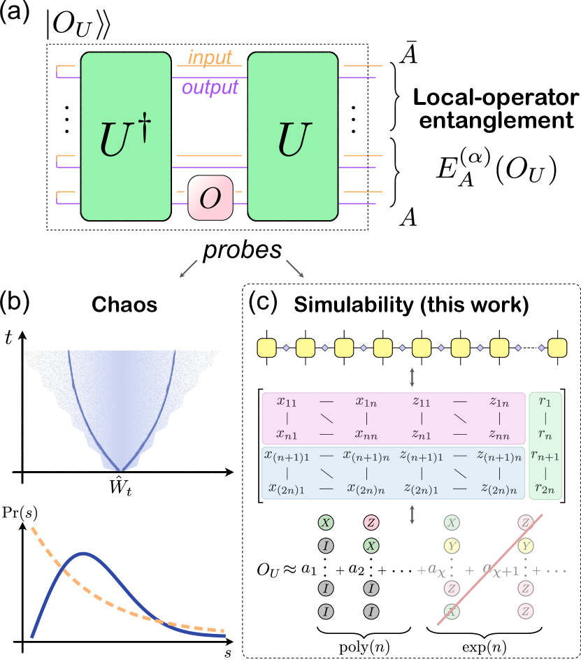
Figure 1: Depiction of of key quantities investigated in this work. (a) The local-operator entanglement (LOE) is the entanglement $E_{A}^{(\alpha)}$ of the Choi state of an operator, $|O_{U}\rangle\!\rangle$, across some (doubled-space) spatial bipartition $A:\bar{A}$ for quantum $\alpha$-Rényi entanglement entropies. (b) The extensive scaling of this quantity witnesses chaos, both in the sense of information scrambling and non-integrability. (c) In addition to being sensitive to entanglement, we show that the LOE equally probes magic resources and operator stabilizer entropies, unifying the three corresponding simulation techniques under the one umbrella.

Here, we pose a new understanding of this relationship. We show that entanglement and magic are conceptually and quantitatively connected. We are able to do this by a shift in perspective from states to operators, noticing that free stabilizer resources are product in operator space. More specifically, consider an operator $O$ in the Heisenberg picture with respect to some evolution $U$, i.e., $O_{U}=U^{\dagger}OU$. By the Choi–Jamiołkowski isomorphism (CJI) $O_{U}$ has a dual pure state, $|O_{U}\rangle\!\rangle:=(O_{U}\otimes\mathds{1})\ket{\phi^{+}}$, where $\ket{\phi^{+}}$ is the (normalized) maximally entangled state on a doubled Hilbert space. Entanglement and magic then have ready generalizations to operators through $|O_{U}\rangle\!\rangle$. The entanglement $E_{A}^{(\alpha)}(O_{U})$ of this state—once appropriately arranged into spatial partitions—is termed the local-operator entanglement (LOE) Prosen and Pižorn (2007), and has been studied in a variety of many-body systems Prosen and Znidarič (2007); Prosen and Pižorn (2007); Pižorn and Prosen (2009); Dubail (2017); Jonay et al. (2018); Alba et al. (2019); Bertini et al. (2020a, b); Alba (2021); see Fig. 1.

Our main result can be succinctly summarized as an upper bound on LOE,

$$E_{A}^{(\alpha)}(O_{U})\leq m,$$ (1)

where $m$ refers to any of three different magic monotones: $T$-count, unitary nullity Jiang and Wang (2023), or operator stabilizer Rényi entropy (OSE) Dowling et al. (2024). Clearly, entangling dynamics are necessary for LOE growth (it is trivially zero for product unitaries). Our result shows that it is not sufficient, and intriguingly that the LOE is limited also by the amount of magic generated by $U$. The quantity therefore represents the interplay between both resources. Moreover, we study the typical behavior of LOE over ensembles with restricted magic resources, finding that this upper bound is approximately saturated for such circuits. The relevant monotones are defined explicitly in Table 1, while the ensembles where the above bound is saturated are depicted in Fig. 2: the well-studied $T$-doped Clifford ensemble Haferkamp et al. (2022a); Leone et al. (2021); Haug et al. (2024), and a $\nu$-compressible ensemble which we introduce in this work.

The above relation Eq. (1) is the subject of the remainder of this work, with the full technical version to be found towards the end of the manuscript (Thm. 2). Our result sits in stark contrast to the corresponding state resource theories, where no such relation exists: states with high magic can be unentangled, while zero-magic (stabilizer) states can have maximal entanglement. Beyond the foundational significance of Eq. (1), there are operational implications. Chaotic dynamical systems have linearly scaling LOE with time, whereas it grows at-fastest logarithmically for integrable dynamics Prosen and Znidarič (2007); Prosen and Pižorn (2007); Pižorn and Prosen (2009); Dubail (2017); Jonay et al. (2018); Alba et al. (2019); Bertini et al. (2020a, b); Alba (2021). Our main result Eq. (1) additionally means that an extensive growth of magic resources is necessary ingredient for quantum chaos (see Cor. 3). Interpreting this result, chaotic growth of LOE implies the impossibility of efficient simulation of those dynamics using standard: tensor network, stabilizer, and Pauli truncation methods (see Cor. 4). LOE therefore serves as a unifying signature of non-classicality.

Average Operator Entanglement from Magic.— Before detailing the full version of Eq. (1) (Thm. 2), we first review the pertinent monotones (summarized in Table 1) and introduce the relevant unitary ensembles (depicted in Fig. 2). Our many-body system of interest $\mathcal{H}$ is an $N$-qubit Hilbert space with total dimension $D=2^{N}$, and denote by $\mathcal{U}_{N}$, $\mathcal{C}_{N}$, and $\mathcal{P}_{N}$ the $N$-qubit unitary, Clifford and Pauli groups respectively. By $U\sim\mathcal{U}_{N}$, we mean that $U$ is sampled uniformly according to the unitarily invariant (Haar) measure on the $N$-qubit unitary group, with an equivalent expression for the Cliffords.

Consider a Heisenberg operator $O_{U}=U^{\dagger}OU$ for some non-trivial initial Pauli operator $O\in\mathcal{P}_{N}\backslash\{\mathds{1}\}$ and a unitary propagator $U$. Through the CJI, the LOE is defined as the bipartite entanglement of the Choi state $|O_{U}\rangle\!\rangle$ across a chosen bipartition $\mathcal{H}=\mathcal{H}_{A}\otimes\mathcal{H}_{\bar{A}}$, $E^{(\alpha)}_{A}(O_{U}):=S^{(\alpha)}(\operatorname{tr}_{\bar{A}}[|O_{U}\rangle\!\rangle\!\langle\!\langle O_{U}|])$, where $S^{(\alpha)}$ represents the (quantum) $\alpha-$Rényi entropy, $S^{(\alpha)}(\rho):=({1-\alpha})^{-1}\log(\operatorname{tr}[\rho^{\alpha}])$. Through abuse of notation, $\operatorname{tr}_{\bar{A}}$ refers to a partial trace over subsystem ${\bar{A}}$ in the doubled space $\mathcal{H}_{\bar{A}}\otimes\mathcal{H}_{\bar{A}}$ with dimension $D_{\bar{A}}^{2}$. We will leave unspecified the exact choice of (spatial) bipartition and Rényi index $\alpha$, unless otherwise stated. When determining the average value of the LOE for classes of circuits, it will also be convenient to study the operator purity of $O_{U}$, defined in the usual way through

$$E^{(\text{pur})}_{A}(O_{U}):=\exp(-E^{(2)}_{A}(O_{U})).$$ (2)

To first provide intuition on the interplay between LOE and magic resources, consider Clifford evolution, $C\in\mathcal{C}_{N}$. It is immediate to see that for any initial Pauli operator $O$ will evolve to some other Pauli operator from the definition of the Clifford group and so the LOE is preserved to be zero. We again stress that no such relation between entanglement and magic holds for states. This invites the question of whether a more quantitative relation can be derived: if a unitary has only a few non-Clifford gates, how does the LOE grow? We will first answer this question by computing the average LOE for ensembles with a tunable magic monotone and show that there is a precise dependence.

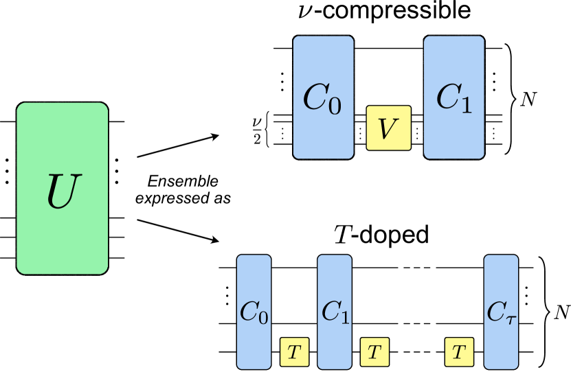
Figure 2: Any unitary can be decomposed as a global Clifford unitaries, $C_{0},C_{1}\in\mathcal{C}_{N}$, sandwiching a non-Clifford unitary on only $\nu(U)/2$ qubits, $V\in\mathcal{U}_{\nu}$ (top), where $\nu(U)$ is the unitary nullity Jiang and Wang (2023). A unitary with $T$-count $\tau(U)$ can be decomposed as layers of $N$-qubit Clifford unitaries $C_{i}\in\mathcal{C}_{N}$ interspersed with $\tau(U)$ single-site $T$-gates (bottom). The $\nu$-compressible and $T$-doped ensembles are constructed from uniformly sampling $\{C_{0},C_{1},V\}$ and $\{C_{i}\}_{0\leq i\leq\tau}$ over the Clifford and unitary groups as appropriate, and are denoted $\mu_{\nu}$ and $\mu_{\tau}$ respectively.

Consider deep Clifford circuits doped with some non-Clifford gates. That is, random Clifford circuits interspersed by $\tau(U)$ single-site $T$-gates, where $\tau(U)$ is the familiar $T$-count magic monotone (see Table 1). If we randomize the Clifford components, such an ensemble of unitaries $\mu_{\tau}$ is called the $T$-doped Clifford ensemble Haferkamp et al. (2022a); Leone et al. (2021) (see Table 1 and Fig. 2). Harnessing Weingarten techniques for averaging over the Clifford group Zhu et al. (2016); Roth et al. (2018); Leone et al. (2021), we can readily compute the operator purity for this example,

$$\int_{U\sim\mu_{\tau}}\!\!\!\!\!\!{E^{(\text{pur})}_{A}(O_{U})}=\exp\left(-\log(\tfrac{4}{3})\tau+\mathcal{O}\left(\frac{({4}/{3})^{\tau}}{D}\right)\right),$$ (3)

where we choose a bipartition of size $N_{A}=N/2$ for the computation of the LOE. The full details of the proof of Eq. (3) (and the below Eq. (6)) can be found in Appendix B, together with exact expressions for arbitrary $\tau(U)$, $N$, and $N_{A}$. Interestingly, the dependence on $(3/4)^{\tau}$ in Eq. (3) is reminiscent of that observed for the linear stabilizer Rényi entropy of the $T-$doped ensemble for large $N$ Leone et al. (2022); Haug et al. (2024). Key for our goals, Eq. (3) shows a linear relationship between $\tau(U)$ and entanglement (recalling Eq. (2)). This result indicates already a proportionality of operator entanglement with magic resources, at least in the typical (average) case. However, while useful practically, it is not always possible to determine the exact $T$-count of a unitary.

Monotone	Definition
LOE	$E^{(\alpha)}_{A}(O_{U}):=S^{(\alpha)}(\operatorname{tr}_{\bar{A}}[|O_{U}\rangle\!\rangle\!\langle\!\langle O_{U}|])$
OSE	$M^{(\alpha)}(O_{U}):=S^{(\alpha)}\!\left(\{\left(\frac{1}{D}\operatorname{tr}[O_{U}P_{i}]\right)^{2}\}_{P_{i}\in\mathcal{P}_{N}}\right)$
Unitary nullity	$\nu(U):=2N-\log_{2}(|\mathrm{Stab}(\ket{U})|)$
$T$-count	Minimum number $\tau(U)$ such that $U=\prod_{i}^{\tau}C_{i}T$, for $C_{i}\in\mathcal{C}_{N}$.

Table 1: Entanglement (first row) and magic (next three rows) monotones that feature in our results. $S^{(\alpha)}$ refers to the $\alpha-$Rényi entropy: its quantum and classical version in the first and second row respectively.

A more concrete magic resource stemming from the algebraic structure of the Clifford group, is the stabilizer nullity Beverland et al. (2020). For quantum states $\ket{\psi}$, this is defined in terms of the cardinality of its stabilizer group: the number of Pauli operators $P$ which satisfy $|\langle\psi|P|\psi\rangle|=1$. The nullity of a unitary operator can be defined analogously Jiang and Wang (2023),

$$\nu(U):=2N-\log_{2}(|\mathrm{Stab}(\ket{U})|).$$ (4)

Here, $\mathrm{Stab}(\ket{U})$ is the stabilizer group of the Choi state $\ket{U}$, equal to $\mathrm{Stab}(\ket{U})=\{P_{1},P_{2}\in\mathcal{P}_{N}:\operatorname{tr}[P_{1}U^{\dagger}P_{2}U]/D=\pm 1\}$. The unitary nullity always takes a non-negative integer value, upper-bounds the largest state nullity of $U$ acting on a stabilizer state, and can be shown to lower-bound the $T$-count Jiang and Wang (2023). Moreover, it gives rise to a powerful representation theorem for any unitary which we present below, building upon previous compressibility results Leone et al. (2024a, b); Gu et al. (2024).

Proposition 1.

Any unitary $U$ with nullity $\nu$ can be decomposed as

$$U=C_{0}(V_{\nu/2}\otimes\mathds{1}_{N-\nu/2})C_{1},$$ (5)

where $C_{0},C_{1}\in\mathcal{C}_{N}$ can act globally, while $V_{\nu/2}\in\mathcal{U}_{\lceil\nu/2\rceil}$ acts on exactly $\lceil\nu(U)/2\rceil$ qubits.

Proof (sketch).

The proof for this follows from the fact that the space spanned by the Paulis in the complement of $\mathrm{Stab}(U)$ (of size $2^{\nu}$), together with their image, can both be mapped to a local space of only $\nu/2$ qubits through pre- and post-processing using Cliffords. Moreover, $P\in\mathrm{Stab}(U)$ can be mapped through the action of another Clifford, which commutes with the non-Clifford part $V$—see App. A. ∎

In contrast to classifying magic in terms of $T$-count, any unitary can be decomposed according to Eq. (5). Of course, for the majority of (high-complexity) unitaries in $\mathcal{U}_{N}$, $\nu(U)=2N$ and so this representation is trivial Poulin et al. (2011). If $\nu(U)<2N$, we call such a unitary $\nu$-compressible. In comparison to similar results presented in Refs. Leone et al. (2024a, b); Gu et al. (2024), Prop. 1 is an improvement through halving the number of qubits in the compression. In particular, Prop. 1 together with a result from Ref. Jiang and Wang (2023) implies that a Clifford circuit with $\tau(U)$ $T$-gates can be compressed to a non-Clifford $V$ acting on at-most $\lceil\tau(U)/2\rceil$ qubits; c.f. Thm. 2 from Ref. Leone et al. (2024b). It is an interesting question to further investigate the implications of this improvement.

Returning to the question of the LOE’s sensitivity to magic resources, we next compute the average-case operator purity for a unitary with a given unitary nullity $\nu(U)$. We define the $\nu$-compressible ensemble of unitaries $\mu_{\nu}$ as that generated from independently randomly sampling $C_{0},C_{1}\in\mathcal{C}_{N}$ and $V\in\mathcal{U}_{\nu/2}$ in Eq. (5) uniformly over the Clifford and unitary groups respectively. Such a unitary ensemble is of indpendent interest, and should find application in other areas of many-body physics. The average operator purity of an initial Pauli $O\in\mathcal{P}_{N}\backslash\{\mathds{1}\}$ for $\nu$-compressible unitaries is

$$\int_{U\sim\mu_{\nu}}\!\!\!{E^{(\text{pur})}_{A}(O_{U})}=\exp\left(\!-\nu+2+\mathcal{O}\left(\frac{1}{4^{\nu}}+\frac{2^{\nu}}{D}\right)\right),$$ (6)

where we use Weingarten techniques for taking Haar averages Collins and Sniady (2006); Zhu et al. (2016); Roth et al. (2018); Mele (2024). Again, via Eq. (2) we observe a linear dependence of operator entanglement with magic monotone $\nu(U)$; c.f. Eq. (1).

Before moving on to an exact bound between LOE and magic resources (without averaging), we would like to compare Eqs. (3) and (6). The ensembles $\mu_{\tau}$ and $\mu_{\nu}$ coincide only for two cases: $\tau=\nu=0$, in which case they correspond uniform measure over Clifford group, and $\tau\to\infty$, $\nu\to 2N$, in which case they correspond to the unitary Haar ensemble. In the former case, as previously discussed, the LOE is trivially equal to zero. In the latter case, we can use our previous results to arrive at a Page-curve-like expression for the average LOE from Haar random dynamics,

$$\int_{U\sim\mathcal{U}_{N}}E^{(\text{pur})}_{A}(O_{U})=\frac{-19+D+2D^{2}}{(1+D)(-9+D^{2})}.$$ (7)

Note that this result generalizes one given in Ref. Kudler-Flam et al. (2021) to beyond only leading order in $1/D$.

Unifying Entanglement and Magic.— We will now show that exact bounds can be derived between these two quantities for arbitrary Rényi indices and any given evolution, resulting in Eq. (1). In order to prove our main result, we first review one further magic monotone. The OSE is defined as the entropy of the distribution of square amplitudes of the Heisenberg operator $O_{U}$ written in the Pauli basis Dowling et al. (2024),

$$M^{(\alpha)}(O_{U}):=(1-\alpha)^{-1}\log\sum_{P\in\mathcal{P}}\left(D^{-1}\operatorname{tr}[O_{U}P]\right)^{2\alpha}.$$ (8)

This quantity generalizes a popular state measure of magic Leone et al. (2022); Haug and Piroli (2023); Leone and Bittel (2024), lower-bounding other magic monotones while satisfying a light-cone bound for local dynamics, and (most pertinent to our results) its scaling dictates the efficiency of Pauli-truncation methods. Using the OSE, together with Prop. 1 and the average-case computations Eqs. (3) and (6), we are now in a position to state our main result (Eq. (1)) in full technical detail.

Theorem 2.

For any $N$-qubit unitary $U$, any initial operator $O\in\mathcal{P}_{N}\backslash\{\mathds{1}\}$, for any $\alpha\geq 0$, any bipartition $\mathcal{H}=\mathcal{H}_{A}\otimes\mathcal{H}_{\bar{A}}$, and any unitary propagator $U$, the LOE $\alpha$-Rényi entropy $E^{(\alpha)}_{A}(O_{U})$ satisfies the following inequalities,

$$F\underset{(\alpha\leq 2)}{\underset{(U\sim\mu)}{\leq}}E^{(\alpha)}_{A}(O_{U})\leq{M}^{(\alpha)}(O_{U})\leq\nu(U)\leq\tau(U),$$ (9)

where the lower bound is valid on average for $\alpha\leq 2$, for sampling over either the $T$-doped Clifford ($\mu_{\tau}$) or $\nu$-compressible ($\mu_{\nu}$) ensembles, and is equal to

$$0\leq F:=\begin{cases}\nu-2-\mathcal{O}\left(\frac{2^{\nu}}{D}+\frac{1}{4^{\nu}}\right),&U\sim\mu_{\nu}\\ \log\!\left(\frac{4}{3}\right)\tau-\mathcal{O}\left(\frac{(4/3)^{\tau}}{D}\right),&U\sim\mu_{\tau}.\end{cases}$$ (10)

Here, $\tau(U)$, $\nu(U)$, and ${M}^{(\alpha)}(O_{U})$ are the $T$-count, unitary nullity, and OSE respectively.

Proof (sketch).

The upper bound is proven through first bounding LOE by OSE, which is apparent from entanglement being the optimum participation entropy over all product bases (with $\mathcal{P}_{N}$ being one such basis). For the remaining two upper-bounds, we use a result from Ref. Jiang and Wang (2023) that $\nu(U)\leq\tau(U)$, and use Prop. 1 to show additionally that OSE lower-bounds the unitary nullity. The lower-bounds on the LOE come directly from Eqs. (3)-(6), after applying Jensen’s inequality for the negative logarithm involved in relating purity to $2-$Rényi entropy, and using the hierarchy of Rényi entropies: $S^{(\alpha)}\leq S^{(\beta)}$ for $\alpha\geq\beta$. The full proof of the upper and lower bounds can be found in Appendices A and B respectively. ∎

Examining both the upper and lower bounds of LOE in Eq. (9), we can see that in the average case for large $N\gg\{\nu,\tau\}\gg 1$, magic resources and operator entanglement approximately coincide. It is instructive to compare Eq. (9) to the equivalent quantities in the Schrödinger picture. Consider the examples of so-called magic states, $\ket{H}^{\otimes N}:=T^{\otimes N}\ket{++\dots+}$ and random stabilizer states, $\ket{\psi_{\mathrm{stab}}}:=C\ket{00\dots 0}$ for some deep circuit $C\sim\mathcal{C}_{N}$. In the first case, the aptly named magic state requires very high magic resources to construct (with a $T$-count and state nullity of $\tau(\ket{T}^{\otimes N})=\nu(\ket{T}^{\otimes N})=N$) but has zero entanglement. On the other hand, a random stabilizer state almost surely has near-maximal entanglement, yet requires no magic resources. The existence of the upper bound Eq. (9) in operator space is therefore striking, pointing towards a unified view of non-classical resources in the Heisenberg picture.

To unpack the operational implications of Thm. 2, we return to the physical meaning of LOE. Exclusively for quantum chaotic dynamics, the LOE has been observed to grow extensively with time, while for integrable dynamics it grows at-fastest logarithmically. This conjecture has been confirmed analytically in free-fermion Hamiltonians Prosen and Znidarič (2007); Prosen and Pižorn (2007); Dubail (2017), the Rule-54 interacting-integrable spin chain Alba et al. (2019), and both integrable and chaotic dual unitary circuit models Bertini et al. (2020a, b), with further supporting numerical evidence to be found in Refs. Pižorn and Prosen (2009); Jonay et al. (2018); Alba (2021). Moreover, fast-growing LOE necessarily indicates that the dynamics are scrambling, as quantified by out-of-time-ordered correlators (OTOCs) Dowling et al. (2023). Within the context of the above, we can interpret Thm. 2 via the necessary growth of OSE, nullity, and $T$-count required to simulate chaotic dynamics.

Corollary 3.

To simulate any chaotic Hamiltonian or Floquet $U_{t}$ parametrized by time $t$, one requires $\mathcal{O}(t)$ non-Clifford resources.

Note that due to its inherent Lieb-Robinson light-cone for the OSE magic monotone (forming the tightest upper bound in Eq. (9)), $\mathcal{O}(t)$ scaling is maximal for local Hamiltonian dynamics Dowling et al. (2024). It is worth comparing the above corollary to the results of Refs. Haferkamp et al. (2022a); Leone et al. (2021). There, it was found that for the $T$-doped Clifford ensemble, $\mathcal{O}(N)$ $T$-gates are both necessary Haferkamp et al. (2022a) and sufficient  Leone et al. (2021) to generate an $\epsilon-$approximate $t$-design, for a sufficiently small error in order to differentiate such randomness using e.g. $8$-point OTOCs. However, these results are valid on-average over unitary ensembles, and so leave open the question of what to expect for deterministic dynamics, such as those generated by some non-integrable spin-chain Hamiltonian. Corollary 3 therefore complements these results to assure us that in fact, quantum chaos really cannot be simulated classically.

To elucidate the preceding statement, from Thm. 2 we can also immediately deduce a hierarchy of computational complexities of simulation using (apparently) inequivalent methods. We consider three prominent techniques in many-body dynamical simulation: the tensor network method of Heisenberg picture time-evolving block decimation (H-TEBD) Hartmann et al. (2009) has a computational cost that scales (exponentially) with LOE Verstraete and Cirac (2006); Schuch et al. (2008); stabilizer methods scale (exponentially) with $T$-count according to the Gottesmann-Knill theorem Gottesman (1998); Aaronson and Gottesman (2004); and Pauli truncation methods which rely on the biased suppression of high-weight Pauli terms in locally noisy/scrambling Heisenberg evolution Rakovszky et al. (2022); Lloyd et al. (2023); Begusic et al. (2024); Srivatsa et al. (2024); Begušić and Chan (2024), and have an expense (exponentially) bounded by the OSE Dowling et al. (2024). Note that these resource costs being large do not preclude the efficient simulation of certain features of a system to polynomial precision, such as the anti-concentration of local observables being well-approximated by either: Pauli-truncating an operator to low OSE Angrisani et al. (2024), or analogously using area-law entangled random tensor-networks Cheng et al. (2024). In the following, if the resource cost $R$ of a simulation method for some one-parameter unitary $U_{t}$ scales extensively with time [layers] $t$, $R(U_{t})\sim\mathcal{O}(t)$, we say that the dynamics [circuit] is non-simulable with respect to the said method.

Corollary 4.

If $U_{t}$ is non-simulable according to H-TEBD, then it is also necessarily non-simulable using Pauli truncation, then it is also necessarily non-simulable using stabilizer methods.

The above result means that if a unitary $U_{t}$ is efficiently simulable according to either stabilizer or Pauli truncation methods, then it must also be efficient to model using H-TEBD.

Conclusion.— The local-operator entanglement of a unitary propagator $U$ has long been conjectured as a faithful measure of quantum chaos, alongside its direct interpretation as tensor network simulability of the dynamics. Here, we have shown through Thm. 2 that this quantity is limited by the minimum of $U$’s entangling capacity and its magic. The implications here are two-fold: we concretely bridge two seemingly discordant resources of fundamental importance in the one quantity. But by extension, our results also integrate a new viewpoint on the non-simulability of complex quantum dynamics.

We emphasize, however, that this work does not rule out the possibility of classically simulating volume-law LOE through other means. For example, matchgate circuits constitute an alternate class of classically tractable systems. Here, Gaussian observables of free-fermionic systems can be computed efficiently  Jozsa and Miyake (2008); Reardon-Smith et al. (2024). Moreover, the relevant class has been observed to display both high entanglement and magic Collura et al. (2024). Nevertheless, we conjecture that a similar relation to the upper bound of Thm 2 will hold in this setting: that LOE can be bounded by the non-Gaussian resources Zhuang et al. (2018) employed. This intuition is bolstered by the observation that LOE grows at fastest logarithmically with time for free-fermionic Hamiltonian evolution Prosen and Znidarič (2007); Prosen and Pižorn (2007); Dubail (2017).

Beyond strict limits, it is important to explore further the behavior of LOE in concrete settings. One way to understand the average-case saturation in Thm. 2 is that typical dynamics are maximally entangling. This makes magic the bottleneck, and thus essentially equivalent to the LOE. Less typical scenarios should also be studied, where the relative amounts of each is on equal footing. Appropriate methods on this front could be found in stabilizer tensor network Masot-Llima and Garcia-Saez (2024); Nakhl et al. (2024) and Clifford-assisted matrix-product state Fux et al. (2024b); Qian et al. (2024) techniques. These combine both stabilizer and tensor network principles to more efficiently simulate certain systems with an intermediate amount of magic resource and may be well-suited to studying LOE in practice. Already, interesting regimes have been numerically identified, such as in Refs. Fux et al. (2024b); Nakhl et al. (2024) it was observed that $T$-doped Clifford circuits can be efficiently simulated up to $\tau\lesssim N$. One might like to investigate more deeply the regimes between the points $m\approx\{0,N,2N\}$ for different magic monotones $m$ and varied entanglement. This is particularly interesting in the context of unitary nullity; c.f. Prop. 1 and the operational power of $\nu$-compressible states studied in Ref. Gu et al. (2024). Understanding such restricted-complexity dynamical systems will offer further insight into quantum randomness Haferkamp et al. (2022a); Leone et al. (2021), simulability Fux et al. (2024b); Nakhl et al. (2024), learnability Leone et al. (2023, 2024b); Gu et al. (2024), and integrability Turkeshi et al. (2024); Tirrito et al. (2024b); Odavic et al. (2024b); Dowling et al. (2024).

Deeply intertwined with the question of dynamical simulability is also that of unitary complexity Nielsen et al. (2006). It is clear that pure-entanglement and pure-magic measures cannot accommodate the linear growth of circuit complexity up to exponential time Haferkamp et al. (2022b). We lastly remark that our results indicate that LOE can be interpreted as a coarse—but better than entanglement or magic alone—measure of circuit complexity, saturating at higher depths. Exploring generalized extensions of the LOE for this topic would be fertile ground for future work.

Appendix A Upper-bounding LOE by magic monotones

In this Appendix, we will prove the upper bound of the main result, Thm. 2. This upper-bound is the cumulation of several theorems which we will supply here. We will first prove the nullity compression result of Prop. 1 and discuss its implications in some more detail. The strategy is then to upper-bound the OSE by the unitary nullity, use that nullity lower-bounds the $T$-count, before proving that OSE further always lower-bounds the LOE of the same Rényi index.

A.1 $\nu$-compressibility of unitaries

First, we restate and prove Prop. 1, on the efficient representation of unitaries with restricted magic resource of unitary nullity. Note that this theorem is similar to that given in Refs. Leone et al. (2024a, b); Gu et al. (2024). See 1

Proof.

A unitary $U$ stabilizes $2^{2N-\nu}$ Pauli strings, mapping them to Paulis. Call this subgroup of Pauli strings $\mathrm{Stab}(U)$. There exists a Clifford $C$ which also does this, such that $\forall P\in\mathrm{Stab}(U)$, $C^{\dagger}PC=U^{\dagger}PU$. Now, for some $V\in\mathcal{U}_{N}$, we can write the unitary as $U=CV$, where $V$ necessarily commutes with all elements of $\mathrm{Stab}(U)$. Therefore, $V$ acts non-trivially only on a space spanned by $2^{\nu}$ Pauli strings, mapping to a space also of dimension $2^{\nu}$ by linearity. Then we can choose pre- and post-processing Cliffords $C_{0}$ and $C_{1}$ which map these input and output spaces respectively to spaces spanned only by local Paulis on the first $\nu/2$ qubits. The factor of $1/2$ comes from the fact that each site has $4$ possible local Paulis (or two independent generators, one corresponding to the input space, and one to the output space). We can freely choose $C_{0}$ and $C_{1}$ to act trivially on $\mathrm{Stab}(U)$. Then together with $C$ above, we arrive at the representation Eq. (5). ∎

The above then directly leads to a well-defined ensemble of unitaries, when randomly sampling $C_{0},C_{1}$ over the Clifford group, and $V$ over the unitary group on a restricted space of $\nu/2$ qubits. When taking replica averages according to $\mu_{\nu}$, the exact location of the $\nu$ qubits that $V$ acts on does not matter, as both the unitary and Clifford groups are invariant under left/right multiplication by permutation operations. The decomposition Prop. 1 and the ensemble $\mu_{\nu}$ are of independent interest, and should find application in other areas of many-body dynamics. As mentioned in the main text, the above improves upon the previous unitary compressibility statements of Refs. Leone et al. (2024a, b); Gu et al. (2024) by a factor of $1/2$. It would be interesting to study Prop. 1 in the context of learnability and gate-complexity, e.g. using similar approaches to Refs. Leone et al. (2024a, b); Gu et al. (2024). For instance, we immediately arrive at an upper-bound on the circuit complexity of any unitary with nullity $\nu(U)$. The circuit complexity of a unitary $g(U)$ is defined as the minimum number of elementary gates required to synthesize a unitary, from some universal gate set Haferkamp et al. (2022b).

Corollary 5.

The circuit complexity of an $N-$qubit $U$ with a unitary nullity of $\nu(U)$, is

$$g(U)=\mathcal{O}(N^{2}+\exp(\nu/2))$$ (11)

Proof.

The above follows immediately from Prop. 1, together with the fact that Clifford unitaries can be compressed to $O(N^{2})$ gates Bravyi and Maslov (2020), whereas arbitrary unitaries can have up to exponential circuit complexity with respect to their support. ∎

Clearly, if the nullity scales logarithmically with $N$, then the unitary necessarily has low (polynomial) circuit complexity. Recalling the bound $\nu(U)\leq\tau(U)$ Jiang and Wang (2023), said another way: circuits with a logarithmic number of non-Clifford gates have a complexity of $\mathcal{O}(N^{2})$, which improves upon the naive scaling of $\mathcal{O}(\log(N)N^{2})$ (which can be deduced from a $T-$doped Clifford circuit representation). Notice that $\mathcal{O}(N^{2})$ scaling is exactly that of Clifford circuits, meaning that a logarithmic number of non-Cliffords do not change the scaling of circuit complexity (albeit the prefators will change).

A.2 Proof of upper bounds

From Prop. 1, we can immediately relate unitary nullity to the OSE.

Proposition 6.

For any initial operator $O\in\mathcal{P}_{N}$ and unitary $U$,

$$\mathcal{M}^{(\alpha)}(O_{U})\leq\nu(U).$$ (12)

Proof.

From Prop. 1, we write the unitary propagator as $U=C_{0}VC_{1}$, where $C\in\mathcal{C}_{N}$, and $V$ is an arbitrary unitary acting on at-most $\lceil\nu(U)/2\rceil\leq N$ qubits. Take $O\in\mathcal{P}_{N}$. Then,

$$U^{\dagger}OU=C_{1}V^{\dagger}C_{0}^{\dagger}OC_{0}VC_{1}=C_{1}V^{\dagger}O^{\prime}VC_{1}$$ (13)

where also $O^{\prime}\in\mathcal{P}_{N}$ by the definition of Clifford unitaries. In the worst case (with respect to maximizing the OSE), the action of $V$ on a Pauli string can output a uniform superposition of at most $4^{\nu/2}$ Pauli strings, as $V$ acts on only $\nu/2$ qubits. The final Clifford conjugation with respect to $C_{1}$ cannot increase the OSE further, as each Pauli string is again mapped to another Pauli. The entropy of a uniform mixture is simply

$$\mathcal{M}^{(\alpha)}\left(\frac{1}{2^{\nu}}\sum^{2^{\nu}}_{i=1}P_{i}\right) =\log(2^{\nu})=\nu.$$ (14)

From this optimal case, the bound of Eq. (12) follows directly. ∎

This result may be of independent interest, as it provides further evidence of the strength of the OSE metric for quantifying the magic of a system.

Now that we have that OSE is always the smallest of the three magic monotones we use in this work (see Table 1), it remains to prove the relation between OSE and LOE.

Lemma 7.

For any Rényi index $\alpha$ and across any bipartition $A:\bar{A}$, local-operator entanglement bounds from below the OSE,

$$E_{A}^{(\alpha)}({O_{U}})\leq M^{(\alpha)}(O_{U}).$$ (15)

Proof.

We first note that the Choi state $|O_{U}\rangle\!\rangle:=(O_{U}\otimes\mathds{1})\ket{\phi^{+}}$ is a normalized pure state. Then the OSE is just the entropy of the coefficients in the (normalized) computational basis of the Choi state $|O_{U}\rangle\!\rangle$,

$$M^{(\alpha)}(O_{U})=\frac{1}{1-\alpha}\log\sum_{P\in\mathcal{P}}\left(D^{-1}\operatorname{tr}[O_{U}P]\right)^{2\alpha}=\frac{1}{1-\alpha}\sum_{P\in\mathcal{P}}|\braket{P|O_{U}}|^{2\alpha}=\frac{1}{1-\alpha}\sum_{i=1}^{4^{N}}|\braket{i|O_{U}}|^{2\alpha}$$ (16)

where the computational basis arises as the Choi states of Pauli operators according to the single-qubit mapping $P_{i}\to\ket{i}$. Here, we have absorbed the normalization $1/\sqrt{D}$ into the expression of the Choi states $|O_{U}\rangle\!\rangle$ and $|P\rangle\!\rangle$, such that they are normalized pure states. Consider an arbitrary bipartition $A:B$. Any pure state (including $|O_{U}\rangle\!\rangle$) can be written as a superposition in terms of some basis $\mathcal{B}$ which is product across this bipartition

$$|O_{U}\rangle\!\rangle=\sum_{j}\lambda_{j}\ket{a_{j}}\ket{b_{j}}.$$ (17)

We call this condition on the basis $\mathcal{B}$ the bipartite-product condition. This is clearly non-unique, and the coefficients $\lambda_{j}$ together with their cardinality are dependent on the choice $\mathcal{B}$. If one dephases with respect to this basis, and then the entropy of the resultant density matrix is

$$S^{(\alpha)}_{\mathcal{B}}(|O_{U}\rangle\!\rangle):=S^{(\alpha)}(\{\lambda_{j}^{2}\}),$$ (18)

where $S^{(\alpha)}$ is the classical $\alpha$-Rényi entropy. We call this the bipartite-basis entropy with respect to $\mathcal{B}$. As a basis which is local everywhere (not just in $A:B$), the Pauli basis clearly satisfies the bipartite-product condition,

$$|O_{U}\rangle\!\rangle=\sum_{i,j}\lambda_{i,j}\ket{i}\ket{j},$$ (19)

and the corresponding entropy $S^{(\alpha)}_{\mathcal{P}}(\ket{O_{t}})$ is the OSE [Eq.(16)]. The Schmidt basis is defined as the unique basis $\mathcal{B}$ satisfying the bipartite-product condition which minimizes the corresponding bipartite-basis entropy. Then the bipartite-basis entropy of the Schmidt basis is just the entanglement entropy, and so lower bounds all other bipartite-basis entropies, including the OSE. ∎

Combining Prop. 6, the fact that $\nu(U)\leq\tau(U)$, and that Lemma 7, we arrive at the hierarchy of upper bounds from Thm. 2,

$$E_{A}^{(\alpha)}({O_{U}})\leq M^{(\alpha)}(O_{U})\leq\nu(U)\leq\tau(U).$$ (20)

Appendix B Average-case lower bound on LOE from unitary ensembles

In this section, we will detail the proofs for the lower bounds of average LOE in terms of magic monotones of nullity and $T$-count, over both the $\nu$-compressible and $T$-doped ensembles.

The key part of these proofs will be the exact computation of the average operator purity, defined as

$$E^{(\text{pur})}(O_{U}):=\operatorname{tr}[\left(\operatorname{tr}_{\bar{A}}(|O_{U}\rangle\!\rangle\bra{O_{U}})\right)^{2}],$$ (21)

i.e. the purity of the Choi stat $|O_{U}\rangle\!\rangle$. Above, we consider operator entanglement to be across any (spatial) bipartition of $\mathcal{H}_{A}\otimes\mathcal{H}_{\bar{A}}$, of $N_{A}$ and $N_{\bar{A}}$ qubits respectively. In the case of both unitary ensembles considered here, the particular qubits in $\mathcal{H}_{A}$ does not matter, only the size $N_{A}$. This is because both the Clifford and unitary groups are invariant under left or right multiplication by a permutation matrix (as permutations are contained in the Clifford group is contained in the unitary group). We can write the operator purity in replica space as

$$E^{(\text{pur})}(O_{U})=\frac{1}{D^{2}}\operatorname{tr}[O_{U}^{\otimes 4}T^{\prime}],$$ (22)

where

$$T^{\prime}:=T_{(1^{A}2^{A})(3^{A}4^{A})(1^{\bar{A}}4^{\bar{A}})(2^{\bar{A}}3^{\bar{A}})}$$ (23)

is a permutation matrix, with $i^{A}$ denoting the $\mathcal{H}_{A}$ subspace of the $i^{th}$ replica space. Eq. (22) is easy to prove graphically, and is part of the standard ‘replica trick’ technique,

$$E^{(\text{pur})}(O_{U})=\operatorname{tr}[\left(\operatorname{tr}_{\bar{A}}(|O_{U}\rangle\!\rangle\!\langle\!\langle O_{U}|)\right)^{2}] =\operatorname{tr}\left[\frac{1}{D}\operatorname{tr}_{\bar{A}}\left(\includegraphics[scale={1.3},valign={c}]{parta.pdf}\right)\frac{1}{D}\operatorname{tr}_{\bar{A}}\left(\includegraphics[scale={1.3},valign={c}]{parta.pdf}\right)\right]$$ (24)

$$=\frac{1}{D^{2}}\operatorname{tr}\left[\,\includegraphics[scale={1.3},valign={c}]{partb.pdf}\,\right]$$ (25)

$$=\frac{1}{D^{2}}\operatorname{tr}\left[\,\includegraphics[scale={1.3},valign={c}]{partc.pdf}\,\right]=\frac{1}{D^{2}}\operatorname{tr}[O_{U}^{\otimes 4}T^{\prime}].$$ (26)

Here, in the first diagram the top two lines represent the (doubled) Hilbert space $\mathcal{H}_{\bar{A}}$, whereas the bottom two wires represent $\mathcal{H}_{{A}}$. The normalization of $(1/D^{2})$ in Eq. (22) comes from the Choi state normalization in Eq. (21).

In the replica form of Eq. (22), the average operator purity takes the form of a $4-$fold average. This can be computed exactly using (generalized) Weingarten calculus. The relevant four-fold unitary (or Clifford) Haar averages contain $(4!)^{2}=576$ terms (from the cardinality of the permutation group), and so post-simplification we will handle these symbolically using Mathematica. Note that the identity of the initial Pauli $O$ does not matter (local or otherwise), as in the case of both ensembles considered, the first random Clifford applied to it essentially randomizes it. In principle, one could use higher moment formulas to compute higher LOE Rényi entropies through the exact expression for the unitary and Clifford commutants Collins and Sniady (2006); Gross et al. (2021). The involved Weingarten calculus becomes much more complex in this case, and we leave it for future work.

From the exact value of the average operator purity (to be computed in the following sections), the proof strategy is to then apply Jensen’s inequality to bound the average $2-$Rényi entropy, and then to apply the hierarchy of Rényi entropy bounds: $S^{(a)}\leq S^{(b)}$ for $a\geq b$, and so a lower bound in terms of $\alpha=2$ is also a lower bound for $\alpha\leq 2$. So in summary

$$-\log(\int_{U}E^{(\text{pur})}(O_{U}))\leq\int_{U}E^{(2)}(O_{U})\leq\int_{U}E^{(1)}(O_{U})$$ (27)

and additionally

$$-\frac{1}{2}\log(\int_{U}E^{(\text{pur})}(O_{U}))\leq\int_{U}E^{(\infty)}(O_{U})$$ (28)

from the bound $E^{(2)}\leq 2E^{(\infty)}$. This final bound can also be used to provide a lower bound in Thm. 2 in terms of Rényi entropies $\alpha>2$, but we do not bother as $S^{(\alpha)}$ for $0\leq\alpha\leq 2$ are more informative Verstraete and Cirac (2006); Schuch et al. (2008).

B.1 Clifford and Haar averages

We will use Weingarten techniques to exactly evaluate $4-$fold averages of the operator purity. We have the following expressions for (i) the four-fold Clifford average Zhu et al. (2016); Roth et al. (2018); Leone et al. (2021),

$$\int_{C\in\mathcal{C}}(C^{\dagger})^{\otimes 4}XC^{\otimes 4}=\sum_{\pi,\sigma\in\mathcal{S}_{4}}\mathrm{Wg}^{+}_{\pi\sigma}\operatorname{tr}[X\Lambda^{+}T_{\pi}]\Lambda^{+}T_{\sigma}+\mathrm{Wg}^{-}_{\pi\sigma}\operatorname{tr}[X\Lambda^{-}T_{\pi}]\Lambda^{-}T_{\sigma},$$ (29)

and (ii) the $4-$fold unitary average Mele (2024),

$$\int_{V\in\mathcal{U}}(V^{\dagger})^{\otimes 4}XV^{\otimes 4}=\sum_{\pi,\sigma\in\mathcal{S}_{4}}\mathrm{Wg}_{\pi\sigma}\operatorname{tr}[XT_{\pi}]T_{\sigma}.$$ (30)

Here, $X\in\mathcal{H}^{\otimes 4}$ lives in $4-$replica space, $\mathcal{S}_{4}$ is the symmetric group, $T_{\pi}$ are permutations, $\Lambda^{\pm}$ are the orthogonal projectors

$$\Lambda^{+}=\frac{1}{D^{2}}\sum_{P\in\mathcal{P}_{N}}P^{\otimes 4};\qquad\Lambda^{-}=\mathds{1}^{\otimes 4}-\Lambda^{+}$$ (31)

which are symmetric under permutations in replica space, and so commute with any $4-$fold Clifford channel. $\mathrm{Wg}^{x}$ are (generalized) Weingarten functions,

$$\mathrm{Wg}^{x}_{\pi\sigma}(D):=\sum_{\lambda\vdash 4,D_{\lambda}^{\pm}\neq 0}\frac{d_{\lambda}^{2}\chi^{\lambda}(\pi\sigma)}{(4!)^{2}D_{\lambda}^{x}}$$ (32)

where $x\in\{+,-,0\}$, and

• $\lambda$ labels the irreducible representations of the symmetric group,

• $d_{\lambda}$ is the dimension of the irreducible representation $\lambda$,

• $\chi^{\lambda}(\pi\sigma)$ are the characters of the symmetric group, and

• $D_{\lambda}^{x}:=\operatorname{tr}[\Lambda^{x}T_{\lambda}]$, where $T_{\lambda}$ are projectors onto the irreducible representation $\lambda$.

Note that the functions $\mathrm{Wg}^{\pm}$ differ from the usual (Haar) Weingarten functions $\mathrm{Wg}^{0}=:\mathrm{Wg}$ only through the factor $D_{\lambda}^{\pm}$, so we can use the usual symbolic tools for Haar integrals. Indeed, we will simply use the table from Lemma 1 in Ref. Zhu et al. (2016) to determine $D_{\lambda}^{\pm}$ and $d_{\lambda}$ in Eq. (32).

As a warm-up before tackling the full computations, we first prove two useful identities.

Lemma 8.

For $O\in\mathcal{P}_{N}$, $T_{\pi}$ the permutation matrix for $\pi\in\mathcal{S}_{4}$, and $\Lambda^{\pm}$ defined as above,

$$\operatorname{tr}[O^{\otimes 4}\Lambda^{+}T_{\pi}]=\operatorname{tr}[\Lambda^{+}T_{\pi}]=D^{\#(\pi)-2\delta_{\pi o}},\text{ and}$$ (33)

$$\operatorname{tr}[O^{\otimes 4}\Lambda^{-}T_{\pi}]=-\delta_{\pi o}D^{\#(\pi)-2},$$ (34)

where $\#(\pi)$ is the number of cycles for the permutation $\pi$, and

$$\delta_{\pi o}=\begin{cases}0&\text{for }\pi\in\mathcal{S}^{e}\;,\\ 1&\text{for }\pi\in\mathcal{S}^{o}\;.\end{cases}$$ (35)

$\mathcal{S}^{e}\subset\mathcal{S}_{4}$ is defined as the ‘even’ permutations, which contain only even cycles, with $\mathcal{S}^{o}\subset\mathcal{S}_{4}$ being the complement (e.g. $(12)(34)$ is even, but $(12)(3)(4)$ is odd).

Proof.

In $\operatorname{tr}[O^{\otimes 4}\Lambda^{\pm}T_{\pi}]$, both $X=O^{\otimes 4}$ and $\Lambda^{\pm}$ are permutation invariant, and so the expression $\operatorname{tr}[X\Lambda^{\pm}T_{\pi}]$ depends only on the cycle structure of $\pi$. Recalling that $\lambda\vdash 4$ is an integer partition of $4$,

$$\operatorname{tr}[O^{\otimes 4}\Lambda^{\pm}T_{\pi}] =\pm\frac{1}{D^{2}}\sum_{P\in\mathcal{P}}\operatorname{tr}[O^{\otimes 4}P^{\otimes 4}T_{\pi}]+\delta_{\pm-}\operatorname{tr}[O^{\otimes 4}T_{\pi}]$$

$$=\pm\frac{1}{D^{2}}\sum_{P\in\mathcal{P}}\prod_{c\in\lambda_{\pi}}\operatorname{tr}[P^{c}]+\delta_{\pm-}\prod_{c\in\lambda_{\pi}}\operatorname{tr}[O^{c}]$$ (36)

where we have also used that left multiplication of Pauli strings in a sum over the full group $\mathcal{P}_{N}$ leaves the sum invariant, as $O\mathcal{P}_{N}=\mathcal{P}_{N}$. Note that any phase is canceled out as there are four copies. The trace in the first term of Eq. (36) depends only on whether the Pauli is identity or not; where if $P\neq\mathds{1}$ then this term is non-zero only for even permutations. Moreover, $O$ is a traceless Pauli, so the second term is non-zero only for permutations $\mathcal{S}^{e}$ solely with cycles of even length. We therefore arrive at

$$\operatorname{tr}[O^{\otimes 4}\Lambda^{\pm}T_{\pi}] =\begin{cases}\pm({D^{2}}/{D^{2}})\prod_{c\in\lambda_{\pi}}\operatorname{tr}[\mathds{1}]+\delta_{\pm-}\prod_{c\in\lambda_{\pi}}\operatorname{tr}[\mathds{1}]&\text{for }\lambda_{\pi}\ni c=2k\;,\\ \pm(1/{D^{2}})\prod_{c\in\lambda_{\pi}}\operatorname{tr}[\mathds{1}]&\text{otherwise}\;,\end{cases}$$ (37)

$$=\begin{cases}\pm D^{\#(\pi)}+\delta_{\pm-}D^{\#(\pi)}&\text{for }\lambda_{\pi}\ni c=2k\;(\pi\in\mathcal{S}^{e}),\\ \pm D^{\#(\pi)-2}&\text{otherwise }(\pi\in\mathcal{S}^{o})\;.\end{cases}$$ (38)

Where $\#(\pi)$ is the number of cycles for the permutation $\pi$. Simplifying this further,

$$\operatorname{tr}[O^{\otimes 4}\Lambda^{+}T_{\pi}]=(D^{\#(\pi)-2\delta_{\pi o}}),$$ (39)

and

$$\operatorname{tr}[O^{\otimes 4}\Lambda^{-}T_{\pi}]=-\delta_{\pi o}(D^{\#(\pi)-2}),$$ (40)

where $\delta_{\pi o}$ is defined in Eq. (35). ∎

Lemma 9.

For a single qubit $Z-$rotation $T$-gate $P_{\pi/4}=\ket{0}\bra{0}+\exp[i\pi/4]\ket{1}\bra{1}$ and $K=P_{\theta}\otimes\mathds{1}_{N-1}$, then

$$\mathrm{tr}\left(K^{\otimes 4}\Lambda^{+}K^{\dagger\otimes 4}T_{\sigma}\right)=D^{\#(\sigma)-2\delta_{\sigma o}},$$ (41)

and,

$$\mathrm{tr}\left(K^{\otimes 4}\Lambda^{+}K^{\dagger\otimes 4}\Lambda^{+}T_{\sigma}\right) =D^{\#(\sigma)-2\delta_{\sigma o}}_{N-1}\frac{1}{2^{4}}\sum_{P_{1},P_{2}\in\mathcal{P}_{1}}\operatorname{tr}[P_{\theta}^{\otimes 4}P_{1}P_{\theta}^{\dagger\otimes 4}P_{2}T_{\sigma}]$$ (42)

$$=:D^{\#(\sigma)-2\delta_{\sigma o}}_{N-1}f_{\sigma}.$$ (43)

This can be directly generalized to other single-qubit non-Cliffords $P_{\theta}$.

Proof.

For the first identity (41), we have

$$\mathrm{tr}\left(K^{\otimes 4}\Lambda^{+}K^{\dagger\otimes 4}T_{\sigma}\right) =\mathrm{tr}\left((P_{\theta}\otimes\mathds{1}_{N-1})^{\otimes 4}\Lambda^{+}(P_{\theta}\otimes\mathds{1}_{N-1})^{\dagger\otimes 4}T_{\sigma}\right)$$ (44)

$$=\frac{1}{2^{2}}\sum_{P_{1}\in\mathcal{P}_{1}}\operatorname{tr}[P_{\theta}^{\otimes 4}P_{1}^{\otimes 4}(P_{\theta}^{\dagger})^{\otimes 4}T_{\sigma}]\operatorname{tr}[\Lambda^{+}_{N-1}T_{\sigma}]$$ (45)

$$=D^{\#(\sigma)-2\delta_{\sigma o}}_{1}D^{\#(\sigma)-2\delta_{\sigma o}}_{N-1}=D^{\#(\sigma)-2\delta_{\sigma o}}.$$ (46)

where we have again used that $\Lambda^{+}$ decomposes into a product operator in replica space, and that $\operatorname{tr}[\Lambda^{+}T_{\sigma}]=D^{\#(\sigma)-2\delta_{\sigma o}}$. Furthermore, for a function $\operatorname{tr}[X^{\otimes 4}T_{\sigma}]$, only the trace properties of $X$ matter, and conjugation by the unitary $P_{\theta}$ preserves the trace (and that $(P_{\theta}P_{1}P_{\theta}^{\dagger})^{2k}=\mathds{1}$). The proof for the second identity (43) first follows a similar method to above,

$$\mathrm{tr}\left(K^{\otimes 4}\Lambda^{+}K^{\dagger\otimes 4}\Lambda^{+}T_{\sigma}\right) =\frac{1}{2^{4}}\sum_{P_{1},P_{2}\in\mathcal{P}_{1}}\operatorname{tr}[P_{\theta}^{\otimes 4}P_{1}^{\otimes 4}(P_{\theta}^{\dagger})^{\otimes 4}P_{2}^{\otimes 4}T_{\sigma}]\operatorname{tr}[\Lambda^{+}_{N-1}\Lambda^{+}_{N-1}T_{\sigma}]$$ (47)

$$=\frac{1}{2^{4}}\sum_{P_{1},P_{2}\in\mathcal{P}_{1}}\operatorname{tr}[P_{\theta}^{\otimes 4}P_{1}^{\otimes 4}(P_{\theta}^{\dagger})^{\otimes 4}P_{2}^{\otimes 4}T_{\sigma}]D^{\#(\sigma)-2\delta_{(\sigma)o}}_{N-1},$$ (48)

where we have again used that $\Lambda^{+}$ decomposes into a product operator, and that it is a projector and so $(\Lambda^{+})^{2}=\Lambda^{+}$. Finally, the factor

$$f_{\sigma}=\frac{1}{2^{4}}\sum_{P_{1},P_{2}\in\mathcal{P}_{1}}\operatorname{tr}[P_{\theta}^{\otimes 4}P_{1}^{\otimes 4}(P_{\theta}^{\dagger})^{\otimes 4}P_{2}^{\otimes 4}T_{\sigma}]$$ (49)

is found from direct computation. ∎

B.2 $\nu$-compressible ensemble

We first consider the $\nu$-compressible ensemble, as it is somewhat simpler to compute than the $T$-doped averages. Recall that the $\nu$-compressible ensemble is defined as the class of unitaries $\{U_{\nu}=C_{0}(V\otimes\mathds{1}_{N-\nu})C_{1}:C_{0/1}\in\mathcal{C}_{N},V\in\mathcal{U}_{\nu}\}$, equipped with the uniform measure over $C_{0},C_{1}\in\mathcal{C}_{N}$ and $V\in\mathcal{U}_{\lceil\nu/2\rceil}$ on the Clifford and unitary groups respectively. For ease of notation, we will write $V\equiv(V\otimes\mathds{1}_{N-\lceil\nu/2\rceil})$ in the following, and write ${\tilde{\nu}}:=\lceil\nu/2\rceil$. As usual, we take initial operator to be a non-identity Pauli string, $O\in\mathcal{P}_{N}\backslash\{\mathds{1}\}$.

Consider the average operator purity over the $\nu$-compressible ensemble. Substituting $U=C_{0}VC_{1}$, we have that

$$\int_{C_{0},C_{1}\in\mathcal{C},V\in\mathcal{U}}E^{(\text{pur})}_{A}(O_{U})=\frac{1}{D^{2}}\operatorname{tr}\left[\left(\int_{C_{0},C_{1}\in\mathcal{C},V\in\mathcal{U}}O_{U}^{\otimes 4}\right)T^{\prime}\right]$$ (50)

where

$$O_{U}=C_{1}^{\dagger}V^{\dagger}C_{0}^{\dagger}OC_{0}VC_{1},$$ (51)

and $T^{\prime}$ is defined in Eq. (23). As each average is independent, we will first perform the Clifford average over $C_{0}$. From Eq. (29), we find that

$$\int_{C_{0}\in\mathcal{C}_{N}}(C_{0}^{\dagger})^{\otimes 4}O^{\otimes 4}C_{0}^{\otimes 4} =\sum_{\zeta,\eta\in\mathcal{S}_{4}}\mathrm{Wg}^{+}_{\zeta\eta}\operatorname{tr}[O^{\otimes 4}\Lambda^{+}T_{\zeta}]\Lambda^{+}T_{\eta}+\mathrm{Wg}^{-}_{\zeta\eta}\operatorname{tr}[O^{\otimes 4}\Lambda^{-}T_{\zeta}]\Lambda^{-}T_{\eta}$$ (52)

$$=\sum_{\zeta,\eta\in\mathcal{S}_{4}}\mathrm{Wg}^{+}_{\zeta\eta}D^{\#(\zeta)-2\delta_{\zeta o}}\Lambda^{+}T_{\eta}-\mathrm{Wg}^{-}_{\zeta\eta}\delta_{\zeta o}D^{\#(\zeta)-2}\Lambda^{-}T_{\eta}$$ (53)

$$=\sum_{\zeta,\eta\in\mathcal{S}_{4}}(\mathrm{Wg}^{+}_{\zeta\eta}+\delta_{\zeta o}\mathrm{Wg}^{-}_{\zeta\eta})D^{\#(\zeta)-2\delta_{\zeta o}}\Lambda^{+}T_{\eta}-\delta_{\zeta o}\mathrm{Wg}^{-}_{\zeta\eta}D^{\#(\zeta)-2}T_{\eta},$$ (54)

where we have used Lemma 8.

For the next averaging over $V\in\mathcal{U}_{\tilde{\nu}}$, we need only consider its effect on the terms $\Lambda^{+}T_{\eta}$ and $T_{\eta}$ from the above Eq. (54), and sub back in the constants and summations at the end. However, the unitary $V$ only acts on ${\tilde{\nu}}$ qubits, with identity elsewhere. Both $\Lambda^{+}T_{\eta}$ and $T_{\eta}$ are product operators within a single replica space, and so

$$\int_{V\in\mathbb{H}}(\mathds{1}\otimes V^{\dagger})^{\otimes 4}\Lambda^{+}T_{\eta}(\mathds{1}\otimes V^{\otimes 4})=\Lambda^{+}T_{\eta}\otimes\int_{V\in\mathbb{H}}(V^{\dagger})^{\otimes 4}\Lambda^{+}T_{\eta}V^{\otimes 4},$$ (55)

where the dimensionality of each $\Lambda^{+}$, $T_{\eta}$ is clear from context: the first term of the tensor product in the final expression acts on $N-{\tilde{\nu}}$ qubits across $4-$replica space, while the second term they act on the remaining ${\tilde{\nu}}$ qubits. Note that the exact identity of this bipartition is irrelevant, as the global Clifford averaging is invariant under left/right multiplication by permutations.

We can then use the usual Haar integration formula, Eq. (30), defining $D_{\tilde{\nu}}:=2^{{\tilde{\nu}}}$ we find that

$$\int_{V\in\mathbb{H}}(V^{\dagger})^{\otimes 4}\Lambda^{+}T_{\eta}V^{\otimes 4}=\sum_{\kappa,\mu\in\mathcal{S}_{4}}\mathrm{Wg}_{\kappa\mu}(D_{\tilde{\nu}})\operatorname{tr}[\Lambda^{+}T_{\eta}T_{\kappa}]T_{\mu}=\sum_{\kappa,\mu\in\mathcal{S}_{4}}\mathrm{Wg}_{\kappa\mu}D_{\tilde{\nu}}^{\#(\eta\kappa)-2\delta_{(\eta\kappa)o}}T_{\mu},\text{ and}$$ (56)

$$\int_{V\in\mathbb{H}}(V^{\dagger})^{\otimes 4}T_{\eta}V^{\otimes 4}=\sum_{\kappa,\mu\in\mathcal{S}_{4}}\mathrm{Wg}_{\kappa\mu}(D_{\tilde{\nu}})\operatorname{tr}[T_{\eta}T_{\kappa}]T_{\mu}=\sum_{\kappa,\mu\in\mathcal{S}_{4}}\mathrm{Wg}_{\kappa\mu}D^{\#(\eta\kappa)}_{\tilde{\nu}}T_{\mu}$$ (57)

where we have again used Lemma 8. We have here in the first equality explicitly included the dimensional dependence of the Weingarten functions, as this Haar average is over a space of ${\tilde{\nu}}$ qubits only. In the following, all Weingarten functions $\mathrm{Wg}_{\pi}=\mathrm{Wg}_{\pi}(D_{\tilde{\nu}})$, whereas all generalized Clifford Weingarten functions have the dependence $\mathrm{Wg}^{\pm}_{\pi}=\mathrm{Wg}_{\pi}^{\pm}(D)$. Substituting this into Eq. (54), we have that

$$\int_{C_{0}\in\mathcal{C}_{N},V\in\mathcal{U}_{\tilde{\nu}}} (V^{\dagger})^{\otimes 4}(C_{0}^{\dagger})^{\otimes 4}O^{\otimes 4}C_{0}^{\otimes 4}V^{\otimes 4}$$ (58)

$$= \sum_{\zeta,\eta\in\mathcal{S}_{4}}(\mathrm{Wg}^{+}_{\zeta\eta}+\delta_{\zeta o}\mathrm{Wg}^{-}_{\zeta\eta})D^{\#(\zeta)-2\delta_{\zeta o}}\Lambda^{+}T_{\eta}\otimes(\sum_{\kappa,\mu\in\mathcal{S}_{4}}\mathrm{Wg}_{\kappa\mu}D_{\tilde{\nu}}^{\#(\eta\kappa)-2\delta_{(\eta\kappa)o}}T_{\mu})$$ (59)

$$-\delta_{\zeta o}\mathrm{Wg}^{-}_{\zeta\eta}D^{\#(\zeta)-2}T_{\eta}\otimes(\sum_{\kappa,\mu\in\mathcal{S}_{4}}\mathrm{Wg}_{\kappa\mu}D^{\#(\eta\kappa)}_{\tilde{\nu}}T_{\mu})$$ (60)

$$= \sum_{\zeta,\eta,\kappa,\mu\in\mathcal{S}_{4}}(\mathrm{Wg}^{+}_{\zeta\eta}+\delta_{\zeta o}\mathrm{Wg}^{-}_{\zeta\eta})\mathrm{Wg}_{\kappa\mu}D^{\#(\zeta)-2\delta_{\zeta o}}D^{\#(\eta\kappa)-2\delta_{(\eta\kappa)o}}_{\tilde{\nu}}(\Lambda^{+}T_{\eta}\otimes T_{\mu})$$ (61)

$$-\delta_{\zeta o}\mathrm{Wg}^{-}_{\zeta\eta}\mathrm{Wg}_{\kappa\mu}D^{\#(\zeta)-2}D^{\#(\eta\kappa)}_{\tilde{\nu}}(T_{\eta}\otimes T_{\mu}).$$ (62)

Here, we stress again that the tensor product $T_{\eta}\otimes T_{\mu}$ is (in-order) on the first $N-{\tilde{\nu}}$ qubits and the next ${\tilde{\nu}}$ qubits respectively (in $4-$replica space).

Now we will perform the final Clifford averaging, over the operators $(\Lambda^{+}T_{\eta}\otimes T_{\mu})$ and $(T_{\eta}\otimes T_{\mu})$ in Eq. (62). We first find that

$$\int_{C_{1}\in\mathcal{C}_{N}}(C_{1}^{\dagger})^{\otimes 4}(T_{\eta}\otimes T_{\mu})C_{1}^{\otimes 4}= \sum_{\pi,\sigma\in\mathcal{S}_{4}}\mathrm{Wg}^{+}_{\pi\sigma}\operatorname{tr}[(T_{\eta}\otimes T_{\mu})\Lambda^{+}T_{\pi}]\Lambda^{+}T_{\sigma}+\mathrm{Wg}^{-}_{\pi\sigma}\operatorname{tr}[(T_{\eta}\otimes T_{\mu})\Lambda^{-}T_{\pi}]\Lambda^{-}T_{\sigma}$$

$$= \sum_{\pi,\sigma\in\mathcal{S}_{4}}\mathrm{Wg}^{+}_{\pi\sigma}D_{N-{\tilde{\nu}}}^{\#(\pi\eta)-2\delta_{(\pi\eta)o}}D_{{\tilde{\nu}}}^{\#(\pi\mu)-2\delta_{(\pi\mu)o}}\Lambda^{+}T_{\sigma}$$

$$+\mathrm{Wg}^{-}_{\pi\sigma}(\operatorname{tr}[(T_{\eta}\otimes T_{\mu})T_{\pi}]-\operatorname{tr}[(T_{\eta}\otimes T_{\mu})\Lambda^{+}T_{\pi}])(\mathds{1}-\Lambda^{+})T_{\sigma}$$

$$= \sum_{\pi,\sigma\in\mathcal{S}_{4}}\mathrm{Wg}^{+}_{\pi\sigma}D_{N-{\tilde{\nu}}}^{\#(\pi\eta)-2\delta_{(\pi\eta)o}}D_{{\tilde{\nu}}}^{\#(\pi\mu)-2\delta_{(\pi\mu)o}}\Lambda^{+}T_{\sigma}$$

$$+\mathrm{Wg}^{-}_{\pi\sigma}(D_{N-{\tilde{\nu}}}^{\#(\pi\eta)}D_{{\tilde{\nu}}}^{\#(\pi\mu)}-D_{N-{\tilde{\nu}}}^{\#(\pi\eta)-2\delta_{(\pi\eta)o}}D_{{\tilde{\nu}}}^{\#(\pi\mu)-2\delta_{(\pi\mu)o}})(\mathds{1}-\Lambda^{+})T_{\sigma}$$

$$= \sum_{\pi,\sigma\in\mathcal{S}_{4}}\left((\mathrm{Wg}^{+}_{\pi\sigma}+\mathrm{Wg}^{-}_{\pi\sigma})D_{N-{\tilde{\nu}}}^{\#(\pi\eta)-2\delta_{(\pi\eta)o}}D_{{\tilde{\nu}}}^{\#(\pi\mu)-2\delta_{(\pi\mu)o}}-\mathrm{Wg}^{-}_{\pi\sigma}D_{N-{\tilde{\nu}}}^{\#(\pi\eta)}D_{{\tilde{\nu}}}^{\#(\pi\mu)}\right)\Lambda^{+}T_{\sigma}$$

$$+\mathrm{Wg}^{-}_{\pi\sigma}(D_{N-{\tilde{\nu}}}^{\#(\pi\eta)}D_{{\tilde{\nu}}}^{\#(\pi\mu)}-D_{N-{\tilde{\nu}}}^{\#(\pi\eta)-2\delta_{(\pi\eta)o}}D_{{\tilde{\nu}}}^{\#(\pi\mu)-2\delta_{(\pi\mu)o}})T_{\sigma}$$ (63)

In the above, we have used that both $\Lambda^{+}$ and $T_{\pi}$ are product operators between qubits: that they factorize into acting independently on the $4-$replica space of the first $N-{\tilde{\nu}}$ qubits, and on the other ${\tilde{\nu}}$ qubits.

Similarly,

$$\int_{C_{1}\in\mathcal{C}_{N}}(C_{1}^{\dagger})^{\otimes 4}(\Lambda^{+}T_{\eta}\otimes T_{\mu})C_{1}^{\otimes 4}= \sum_{\pi,\sigma\in\mathcal{S}_{4}}\mathrm{Wg}^{+}_{\pi\sigma}\operatorname{tr}[(\Lambda^{+}T_{\eta}\otimes T_{\mu})\Lambda^{+}T_{\pi}]\Lambda^{+}T_{\sigma}+\mathrm{Wg}^{-}_{\pi\sigma}\operatorname{tr}[(\Lambda^{+}T_{\eta}\otimes T_{\mu})\Lambda^{-}T_{\pi}]\Lambda^{-}T_{\sigma}$$

$$= \sum_{\pi,\sigma\in\mathcal{S}_{4}}\mathrm{Wg}^{+}_{\pi\sigma}D_{N-{\tilde{\nu}}}^{\#(\pi\eta)-2\delta_{(\pi\eta)o}}D_{{\tilde{\nu}}}^{\#(\pi\mu)-2\delta_{(\pi\mu)o}}\Lambda^{+}T_{\sigma}$$

$$+\mathrm{Wg}^{-}_{\pi\sigma}(D_{N-{\tilde{\nu}}}^{\#(\pi\eta)-2\delta_{(\pi\eta)o}}D_{{\tilde{\nu}}}^{\#(\pi\mu)}-D_{N-{\tilde{\nu}}}^{\#(\pi\eta)-2\delta_{(\pi\eta)o}}D_{{\tilde{\nu}}}^{\#(\pi\mu)-2\delta_{(\pi\mu)o}})(\mathds{1}-\Lambda^{+})T_{\sigma}$$

$$= \sum_{\pi,\sigma\in\mathcal{S}_{4}}\left((\mathrm{Wg}^{+}_{\pi\sigma}+\mathrm{Wg}^{-}_{\pi\sigma})D_{N-{\tilde{\nu}}}^{\#(\pi\eta)-2\delta_{(\pi\eta)o}}D_{{\tilde{\nu}}}^{\#(\pi\mu)-2\delta_{(\pi\mu)o}}-\mathrm{Wg}^{-}_{\pi\sigma}D_{N-{\tilde{\nu}}}^{\#(\pi\eta)-2\delta_{(\pi\eta)o}}D_{{\tilde{\nu}}}^{\#(\pi\mu)}\right)\Lambda^{+}T_{\sigma}$$

$$+\mathrm{Wg}^{-}_{\pi\sigma}(D_{N-{\tilde{\nu}}}^{\#(\pi\eta)-2\delta_{(\pi\eta)o}}D_{{\tilde{\nu}}}^{\#(\pi\mu)}-D_{N-{\tilde{\nu}}}^{\#(\pi\eta)-2\delta_{(\pi\eta)o}}D_{{\tilde{\nu}}}^{\#(\pi\mu)-2\delta_{(\pi\mu)o}})T_{\sigma}$$ (64)

Here, we have used that $\Lambda^{+}$ is a projector, and so $(\Lambda^{+})^{2}=\Lambda^{+}$. This means that the above is almost identical to Eq. (63), expect for the factor proportional to $\operatorname{tr}[(\Lambda^{+}T_{\eta}\otimes T_{\mu})T_{\pi}]$.

Now, it remains to substitute the full (triple-)average over Clifford, then unitary, then Clifford groups, into the expression for operator purity, Eq. (50). Recalling the definition of the purity-permutation $T^{\prime}$ in Eq. (23), from Eq. (64) we simply need to compute $\operatorname{tr}[T_{\sigma}T^{\prime}]$ and $\operatorname{tr}[\Lambda^{+}T_{\sigma}T^{\prime}]$, as everything else in our expression is a constant. Again utilizing that permutations and the projector $\Lambda^{+}$ are product operators between qubits, we find that,

$$\operatorname{tr}[\Lambda^{+}T_{\sigma}T^{\prime}] =\frac{1}{D^{2}}\sum_{\begin{subarray}{c}P_{1}\in\mathcal{P}_{A}\\ P_{2}\in\mathcal{P}_{\bar{A}}\end{subarray}}\operatorname{tr}[P_{1}T_{\sigma}T_{(12)(34)}]\operatorname{tr}[P_{2}T_{\sigma}T_{(14)(23)}]$$ (65)

$$=\begin{cases}D_{A}^{\#(\sigma{(12)(34)})}D_{\bar{A}}^{\#(\sigma{(14)(23)})}&\text{for }\sigma{(12)(34)},\,\sigma{(14)(23)}\in\mathcal{S}^{e}\;,\\ D_{A}^{\#(\sigma{(12)(34)})}D_{\bar{A}}^{\#(\sigma{(14)(23)})-2}&\text{for }\sigma{(12)(34)}\in\mathcal{S}^{e},\sigma{(14)(23)}\in\mathcal{S}^{o}\;,\\ D_{A}^{\#(\sigma{(12)(34)})-2}D_{\bar{A}}^{\#(\sigma{(14)(23)})}&\text{for }\sigma{(12)(34)}\in\mathcal{S}^{o},\sigma{(14)(23)}\in\mathcal{S}^{e}\;,\\ D_{A}^{\#(\sigma{(12)(34)})-2}D_{\bar{A}}^{\#(\sigma{(14)(23)})-2}&\text{for }\sigma{(12)(34)},\,\sigma{(14)(23)}\in\mathcal{S}^{o}\;.\end{cases}$$ (66)

$$=D_{A}^{\#(\sigma{(12)(34)})-2\delta_{(\sigma{(12)(34)})o}}D_{\bar{A}}^{\#(\sigma{(14)(23)})-2\delta_{(\sigma{(14)(23)})o}}.$$ (67)

Similarly,

$$\operatorname{tr}[T_{\sigma}T^{\prime}]=D_{A}^{\#(\sigma(12)(34))}D_{\bar{A}}^{\#(\sigma(14)(23))}.$$ (68)

To obtain our final expression, we use Eqs. (66)-(68) to give the action of the final trace with respect to $T^{\prime}$ in Eqs. (63)-(64), and then use these to give the final $4-$fold Clifford averaging of Eq. (62). Remembering the $1/D^{2}$ overall normalization in the operator purity Eq. (22), we arrive at

$$\int_{C_{0},C_{1}\in\mathcal{C},V\in\mathcal{U}}E^{(\text{pur})}_{A}= \frac{1}{D^{2}}\sum_{\zeta,\eta,\kappa,\mu,\pi,\sigma\in\mathcal{S}_{4}}(\mathrm{Wg}^{+}_{\zeta\eta}+\delta_{\zeta o}\mathrm{Wg}^{-}_{\zeta\eta})\mathrm{Wg}_{\kappa\mu}D^{\#(\zeta)-2\delta_{\zeta o}}D^{\#(\eta\kappa)-2\delta_{(\eta\kappa)o}}_{\tilde{\nu}}$$

$$\times\Bigg{(}\left((\mathrm{Wg}^{+}_{\pi\sigma}+\mathrm{Wg}^{-}_{\pi\sigma})D_{N-{\tilde{\nu}}}^{\#(\pi\eta)-2\delta_{(\pi\eta)o}}D_{{\tilde{\nu}}}^{\#(\pi\mu)-2\delta_{(\pi\mu)o}}-\mathrm{Wg}^{-}_{\pi\sigma}D_{N-{\tilde{\nu}}}^{\#(\pi\eta)-2\delta_{(\pi\eta)o}}D_{{\tilde{\nu}}}^{\#(\pi\mu)}\right)$$

$$\times D_{A}^{\#(\sigma{(12)(34)})-2\delta_{(\sigma{(12)(34)})o}}D_{\bar{A}}^{\#(\sigma{(14)(23)})-2\delta_{(\sigma{(14)(23)})o}}$$

$$+\mathrm{Wg}^{-}_{\pi\sigma}(D_{N-{\tilde{\nu}}}^{\#(\pi\eta)-2\delta_{(\pi\eta)o}}D_{{\tilde{\nu}}}^{\#(\pi\mu)}-D_{N-{\tilde{\nu}}}^{\#(\pi\eta)-2\delta_{(\pi\eta)o}}D_{{\tilde{\nu}}}^{\#(\pi\mu)-2\delta_{(\pi\mu)o}})D_{A}^{\#(\sigma(12)(34))}D_{\bar{A}}^{\#(\sigma(14)(23))}\Bigg{)}$$

$$-\delta_{\zeta o}\mathrm{Wg}^{-}_{\zeta\eta}\mathrm{Wg}_{\kappa\mu}D^{\#(\zeta)-2}D^{\#(\eta\kappa)}_{\tilde{\nu}}\Bigg{(}\Big{(}(\mathrm{Wg}^{+}_{\pi\sigma}+\mathrm{Wg}^{-}_{\pi\sigma})D_{N-{\tilde{\nu}}}^{\#(\pi\eta)-2\delta_{(\pi\eta)o}}D_{{\tilde{\nu}}}^{\#(\pi\mu)-2\delta_{(\pi\mu)o}}$$

$$-\mathrm{Wg}^{-}_{\pi\sigma}D_{N-{\tilde{\nu}}}^{\#(\pi\eta)}D_{{\tilde{\nu}}}^{\#(\pi\mu)}\Big{)}D_{A}^{\#(\sigma{(12)(34)})-2\delta_{(\sigma{(12)(34)})o}}D_{\bar{A}}^{\#(\sigma{(14)(23)})-2\delta_{(\sigma{(14)(23)})o}}$$

$$+\mathrm{Wg}^{-}_{\pi\sigma}(D_{N-{\tilde{\nu}}}^{\#(\pi\eta)}D_{{\tilde{\nu}}}^{\#(\pi\mu)}-D_{N-{\tilde{\nu}}}^{\#(\pi\eta)-2\delta_{(\pi\eta)o}}D_{{\tilde{\nu}}}^{\#(\pi\mu)-2\delta_{(\pi\mu)o}})D_{A}^{\#(\sigma(12)(34))}D_{\bar{A}}^{\#(\sigma(14)(23))}\Bigg{)}$$ (69)

$$= \frac{16^{-{\tilde{\nu}}}}{\left(-9+4^{\tilde{\nu}}\right)\left(-4+D^{2}\right)\left(-1+D^{2}\right)^{2}D_{A}^{2}}\Bigg{(}24D^{4}\left(d-d_{A}\right)\left(d+d_{A}\right)\left(-1+d_{A}^{2}\right)$$

$$-4^{1+{\tilde{\nu}}}D^{2}\left(-4+9D^{2}\right)\left(D-D_{A}\right)\left(D+D_{A}\right)\left(-1+D_{A}^{2}\right)$$

$$+16^{\tilde{\nu}}\big{(}18D^{4}-13D^{6}+\left(36-99D^{2}+49D^{4}+4D^{6}\right)D_{A}^{2}+D^{2}\left(18-13D^{2}\right)D_{A}^{4}\big{)}$$

$$+64^{\tilde{\nu}}\big{(}D^{6}-4D_{A}^{2}+D^{2}D_{A}^{2}\left(11-2D_{A}^{2}\right)+D^{4}\left(-2-5D_{A}^{2}+D_{A}^{4}\right)\big{)}\Bigg{)}.$$

This was computed symbolically in Mathematica. The above is a generalization of Eq. (6) presented in the main text; it is valid for any $D$, $\nu$, and $D_{A}$. We will now explore various limits of this quantity to extract some physical insight.

First consider ${\tilde{\nu}}=N$. Our answer should agree with the Haar averaged LOE, as the Cliffords $C_{0},C_{1}$ will have no effect in this case: Clifford twirling a Haar twirl leaves the Haar twirl invariant, due to the unitary invariance of the Haar measure.

Corollary 10.

For a Haar random unitary $V$, the average Heisenberg operator purity is

$$\int_{V\in\mathcal{U}_{N}}E^{(\text{pur})}_{A}(V^{\dagger}OV)=\lim_{{\tilde{\nu}}\to N}\int_{C_{0},C_{1}\in\mathcal{C}_{N},V\in\mathcal{U}_{\tilde{\nu}}}E^{(\text{pur})}_{A} =\frac{(D^{4}_{A}+D^{2})(D^{2}-10)-D_{A}^{2}(D^{2}-19)}{D_{A}^{2}(D^{2}-9)(D^{2}-1)}$$ (70)

$$=\frac{1}{D_{A}^{2}}+\frac{1}{D_{\bar{A}}^{2}}+\mathcal{O}(\frac{1}{D}).$$ (71)

where the final equality is written to leading order in $1/D$.

Note that the final expression agrees with the leading order term for the Haar averaged operator purity from Ref. Kudler-Flam et al. (2021) (see Eq. (29)). Moreover, choosing an equal-sized bipartition of $D_{A}=\sqrt{D}$, we arrive at Eq. (7) in the main text.

Now consider the limit $D_{A}=\sqrt{D}$ for arbitrary $\nu$, to get the simpler expression,

$$\int_{C_{0},C_{1}\in\mathcal{C}_{N},V\in\mathcal{U}_{\tilde{\nu}}}E^{(\text{pur})}_{N_{A}=N/2}(O_{U})= \frac{16^{-{\tilde{\nu}}}}{\left(-9+4^{\tilde{\nu}}\right)\left(1+D\right)^{2}\left(-4+D^{2}\right)}\Bigg{(}24D^{4}-4^{1+{\tilde{\nu}}}D^{2}\left(-4+9D^{2}\right)$$ (72)

$$+64^{\tilde{\nu}}\big{(}-4+D\left(-8+D\left(-1+2D\right)\right)\big{)}+16^{\tilde{\nu}}\big{(}36+D\left(72+D\left(9+2D\left(-9+2D\right)\right)\right)\big{)}\Bigg{)}.$$

Taking the leading and subleading order expression in large $D$, we arrive at

$$\int_{C_{0},C_{1}\in\mathcal{C}_{N},V\in\mathcal{U}_{\tilde{\nu}}}E^{(\text{pur})}_{N_{A}=N/2}(O_{U}) \approx\frac{4D_{\tilde{\nu}}^{4}-36D_{\tilde{\nu}}^{2}+24}{D_{\tilde{\nu}}^{4}(D_{\tilde{\nu}}^{2}-9)}+\frac{2D_{\tilde{\nu}}^{2}-18}{D_{\tilde{\nu}}^{2}-9}\left(\frac{1}{D}\right)+\mathcal{O}\left(\frac{1}{D^{2}}\right)$$ (73)

$$=\frac{4}{D_{\tilde{\nu}}^{2}}+\frac{24}{D_{\tilde{\nu}}^{4}(D_{\tilde{\nu}}^{2}-9)}+\frac{2}{D}+\mathcal{O}\left(\frac{1}{D^{2}}\right)$$ (74)

Here, we have neglected factors proportional to $1/D^{2}$. To obtain a lower bound as that which appears in Thm. 2, we apply Jensen’s inequality,

$$-\log\left[\int_{C_{0},C_{1}\in\mathcal{C}_{N},V\in\mathcal{U}_{\tilde{\nu}}}E^{(\text{pur})}_{N_{A}=N/2}(O_{U})\right]\leq\int_{C\in\mathcal{C},V\in\mathbb{H}}E^{(2)}_{N_{A}=N/2}(O_{U})$$ (75)

and so after some simplification, (also recalling that $D_{\nu}=2^{\nu/2}$),

$$\nu-2-\log\left(1+\frac{6}{D_{\tilde{\nu}}^{4}(D_{\tilde{\nu}}^{2}-9)}+\mathcal{O}(D_{\tilde{\nu}}^{2}/D)\right)\leq\int_{C_{0},C_{1}\in\mathcal{C}_{N},V\in\mathcal{U}_{\tilde{\nu}}}E^{(2)}_{N/2}$$ (76)

$$\implies \nu-2-\mathcal{O}\left(2^{-2\nu}+2^{\nu-N}\right)\leq\int_{C_{0},C_{1}\in\mathcal{C}_{N},V\in\mathcal{U}_{\nu/2}}E^{(2)}_{N_{A}=N/2}$$ (77)

where the final line is an approximation for small $\frac{D_{\nu}^{2}}{D}+\frac{1}{D_{\nu}^{2}}$. The exponential of the negative of the LHS is exactly the result of Eq. (6).

B.3 $T$-doped Clifford ensemble

We first restate the result from Ref. Leone et al. (2021) (based on results from Zhu et al. (2016)):

Theorem 11.

(Leone et al. (2021)) For the set of $T$-doped Clifford circuits $\mathcal{C}_{\tau}$ with $\tau$ $T$-gates, the uniform $4-$fold average over some four-replica quantity $X\in\mathcal{H}^{\otimes 4}$ is

$$\Phi^{(4)}_{\mathcal{C}_{\tau}}(X)=\sum_{\pi,\sigma\in\mathcal{S}_{4}}\left[\left((\Xi^{\tau})_{\pi\sigma}\Lambda^{+}+\Gamma^{(\tau)}_{\pi\sigma}\right)c_{\pi}(X)+\delta_{\pi\sigma}b_{\pi}(X)\right]T_{\sigma}$$ (78)

where $\Lambda^{\pm}$ are defined as in Eq. (31),

$$\Xi_{\sigma\pi}\equiv\sum_{\mu\in S_{4}}\left[\mathrm{Wg}^{+}_{\pi\mu}\mathrm{tr}\left(T_{\sigma}K^{\otimes 4}\Lambda^{+}K^{\dagger\otimes 4}\Lambda^{+}T_{\mu}\right)-\mathrm{Wg}^{-}_{\pi\mu}\mathrm{tr}\left(T_{\sigma}K^{\otimes 4}\Lambda^{+}K^{\dagger\otimes 4}\Lambda^{-}T_{\mu}\right)\right]$$ (79)

with

$$\Gamma^{(\tau)}_{\pi\sigma}=\sum_{\mu\in S_{4}}F_{\pi\mu}\sum_{i=0}^{\tau-1}(\Xi^{i})_{\mu\sigma}$$ (80)

$$F_{\pi\mu}=\sum_{\sigma\in S_{4}}\mathrm{Wg}^{-}_{\pi\sigma}\mathrm{tr}\left(K^{\otimes 4}\Lambda^{+}K^{\dagger\otimes 4}\Lambda^{-}T_{\sigma\mu}\right)$$ (81)

and the information about $X$ is contained in the coefficients (from the first Clifford averaging)

$$c_{\pi}(X)=\sum_{\sigma\in S_{4}}\left[\mathrm{Wg}^{+}_{\pi\sigma}\mathrm{tr}(X\Lambda^{+}T_{\sigma})-\mathrm{Wg}^{-}_{\pi\sigma}\operatorname{tr}[X\Lambda^{-}T_{\sigma}]\right]$$ (82)

$$b_{\pi}(X)=\sum_{\sigma\in S_{4}}\mathrm{Wg}^{-}_{\pi\sigma}\mathrm{tr}(X\Lambda^{-}T_{\sigma}).$$ (83)

For our purposes, the quantity of interest is the operator purity,

$$\int_{U\in\mathcal{C}_{\tau}}E^{(\text{pur})}_{A}=\frac{1}{D^{2}}\int_{U\in\mathcal{C}_{\tau}}\operatorname{tr}[(U^{\dagger})^{\otimes 4}O^{\otimes 4}U^{\otimes 4}T^{\prime}]=\frac{1}{D^{2}}\operatorname{tr}[\Phi^{(4)}_{\mathcal{C}_{\tau}}(O^{\otimes 4})T^{\prime}].$$ (84)

As earlier, the first step involves a global Clifford average, so the identity of the initial operator $O$ (beyond it being a traceless Pauli string) is irrelevant. As a first step, we simplify the coefficients using Lemma 8

$$c_{\pi}(O^{\otimes 4}) =\sum_{\sigma\in S_{4}}\left[\mathrm{Wg}^{+}_{\pi\sigma}\mathrm{tr}(O^{\otimes 4}\Lambda^{+}T_{\sigma})-\mathrm{Wg}^{-}_{\pi\sigma}\mathrm{tr}(O^{\otimes 4}\Lambda^{-}T_{\sigma})\right]$$ (85)

$$=\sum_{\sigma\in S_{4}}\left[(\mathrm{Wg}^{+}_{\pi\sigma}+\mathrm{Wg}^{-}_{\pi\sigma})\frac{1}{D^{2}}\sum_{P\in\mathcal{P}_{N}}\mathrm{tr}(O^{\otimes 4}P^{\otimes 4}T_{\sigma})-\mathrm{Wg}^{-}_{\pi\sigma}\mathrm{tr}(O^{\otimes 4}T_{\sigma})\right]$$ (86)

$$=\sum_{\sigma\in S_{4}}\left[(\mathrm{Wg}^{+}_{\pi\sigma}+\mathrm{Wg}^{-}_{\pi\sigma})D^{\#(\sigma)-2\delta_{\sigma o}}-\mathrm{Wg}^{-}_{\pi\sigma}\delta_{\sigma e}D^{\#(\sigma)}\right],$$ (87)

where we have used the $\delta_{\sigma o}$ notation defined in Eq. (35). Similarly,

$$b_{\pi}(O^{\otimes 4})=\sum_{\sigma\in S_{4}}\left[\mathrm{Wg}^{-}_{\pi\sigma}\delta_{\sigma e}D^{\#(\sigma)}-\mathrm{Wg}^{-}_{\pi\sigma}D^{\#(\sigma)-2\delta_{\sigma o}}\right]=-\sum_{\sigma\in S_{o}}\mathrm{Wg}^{-}_{\pi\sigma}D^{\#(\sigma)-2}.$$ (88)

Now, for the matrix $F$, we assume that $K$ is a single qubit $R^{Z}_{\theta}$ gate wlog acting on the first qubit, which we call $P_{\theta}$. For the rest of the proof, we will use the Lemmas 8-9.

Now, we will consider each of the factors in Lemma 11. Directly applying the Lemma 9 to the matrix $F$, we find

$$F_{\pi\mu}= \sum_{\sigma\in S_{4}}\mathrm{Wg}^{-}_{\pi\sigma}\mathrm{tr}\left(K^{\otimes 4}\Lambda^{+}K^{\dagger\otimes 4}\Lambda^{-}T_{\sigma\mu}\right)$$ (89)

$$= \sum_{\sigma\in S_{4}}\mathrm{Wg}^{-}_{\pi\sigma}\left(\mathrm{tr}[K^{\otimes 4}\Lambda^{+}K^{\dagger\otimes 4}T_{\sigma\mu}]-\mathrm{tr}[K^{\otimes 4}\Lambda^{+}K^{\dagger\otimes 4}\Lambda^{+}T_{\sigma\mu}]\right)$$ (90)

$$= \sum_{\sigma\in S_{4}}\mathrm{Wg}^{-}_{\pi\sigma}(D^{\#(\sigma\mu)-2\delta_{(\sigma\mu)o}}-D^{\#(\sigma\mu)-2\delta_{(\sigma\mu)o}}_{N-1}f_{(\sigma\mu)}).$$ (91)

The factor $f_{(\sigma\mu)}$ can be found through direct calculation, as it is only a single-qubit trace equation. Then, also directly,

$$\Xi_{\sigma\pi} =\sum_{\mu\in S_{4}}\left[\mathrm{Wg}^{+}_{\pi\mu}\mathrm{tr}\left(K^{\otimes 4}\Lambda^{+}K^{\dagger\otimes 4}\Lambda^{+}T_{\mu\sigma}\right)-\mathrm{Wg}^{-}_{\pi\mu}\mathrm{tr}\left(K^{\otimes 4}\Lambda^{+}K^{\dagger\otimes 4}\Lambda^{-}T_{\mu\sigma}\right)\right]$$ (92)

$$=\sum_{\mu\in S_{4}}\left[(\mathrm{Wg}^{+}_{\pi\mu}+\mathrm{Wg}^{-}_{\pi\mu})\mathrm{tr}\left(K^{\otimes 4}\Lambda^{+}K^{\dagger\otimes 4}\Lambda^{+}T_{\mu\sigma}\right)-\mathrm{Wg}^{-}_{\pi\mu}\mathrm{tr}\left(K^{\otimes 4}\Lambda^{+}K^{\dagger\otimes 4}T_{\mu\sigma}\right)\right]$$ (93)

$$=\sum_{\mu\in S_{4}}\left[(\mathrm{Wg}^{+}_{\pi\mu}+\mathrm{Wg}^{-}_{\pi\mu})D^{\#(\mu\sigma)-2\delta_{(\mu\sigma)o}}_{N-1}f_{(\mu\sigma)}-\mathrm{Wg}^{-}_{\pi\mu}D^{\#(\mu\sigma)-2\delta_{(\mu\sigma)o}}\right].$$ (94)

We can exactly diagonalize this $24\times 24$ matrix symbolically to perform arbitrary matrix powers in the full expression (78).

Finally, for the ‘outside’ terms, we have the factors

$$\operatorname{tr}[\Lambda^{+}T_{\sigma}T^{\prime}]=D_{A}^{\#(\sigma{(12)(34)})-2\delta_{(\sigma{(12)(34)})o}}D_{\bar{A}}^{\#(\sigma{(14)(23)})-2\delta_{(\sigma{(14)(23)})o}}$$ (95)

and

$$\operatorname{tr}[T_{\sigma}T^{\prime}]=D_{A}^{\#(\sigma{(12)(34)})}D_{\bar{A}}^{\#(\sigma{(14)(23)})},$$ (96)

which we solved for in Eqs. (66)-(68).

Putting this all together, we have

$$\int_{U\in\mathcal{C}_{\tau}}E^{(\text{pur})}_{A}=\frac{1}{D^{2}}\operatorname{tr}[\sum_{\pi,\sigma\in\mathcal{S}_{4}}\left[\left((\Xi^{\tau})_{\pi\sigma}\Lambda^{+}+\Gamma^{(\tau)}_{\pi\sigma}\right)c_{\pi}(X)+\delta_{\pi\sigma}b_{\pi}(X)\right]T_{\sigma}T^{\prime}]$$

$$\quad=\frac{1}{D^{2}}\Big{(}\sum_{\pi,\sigma\in\mathcal{S}_{4}}\Big{[}\big{(}(\Xi^{\tau})_{\pi\sigma}\underbrace{D_{A}^{\#(\sigma{(12)(34)})-2\delta_{(\sigma{(12)(34)})o}}D_{\bar{A}}^{\#(\sigma{(14)(23)})-2\delta_{(\sigma{(14)(23)})o}}}_{\operatorname{tr}[\Lambda^{+}T_{\sigma}T^{\prime}]}$$

$$\quad+\sum_{\kappa\in S_{4}}\underbrace{\sum_{\zeta\in S_{4}}\mathrm{Wg}^{-}_{\pi\zeta}(D^{\#(\zeta\kappa)-2\delta_{(\zeta\kappa)o}}-D^{\#(\zeta\kappa)-2\delta_{(\zeta\kappa)o}}_{N-1}f_{(\zeta\kappa)})}_{F_{\pi\kappa}}\sum_{i=0}^{\tau-1}(\Xi^{i})_{\kappa\sigma}\underbrace{D_{A}^{\#(\sigma{(12)(34)})}D_{\bar{A}}^{\#(\sigma{(14)(23)})}}_{\operatorname{tr}[T_{\sigma}T^{\prime}]}\Big{]}$$ (97)

$$\quad\times\underbrace{\sum_{\mu\in S_{4}}\left[(\mathrm{Wg}^{+}_{\pi\mu}+\mathrm{Wg}^{-}_{\pi\mu})D^{\#(\mu)-2\delta_{\mu o}}-\mathrm{Wg}^{-}_{\pi\mu}\delta_{\mu e}D^{\#(\mu)}\right]}_{c_{\pi}(O^{\otimes 4})}-\delta_{\pi\sigma}\underbrace{\left[\sum_{\kappa\in S_{o}}\mathrm{Wg}^{-}_{\pi\kappa}D^{\#(\kappa)-2}\right]D_{A}^{\#(\sigma{(12)(34)})}D_{\bar{A}}^{\#(\sigma{(14)(23)})}}_{b_{\pi}(O^{\otimes 4})\operatorname{tr}[T_{\sigma}T^{\prime}]}\Big{)}$$

Evaluating this symbolically, for the case of $N_{A}=N/2$ (the arbitrary $N_{A}$ case is too long and complex to report here), we arrive at

$$\int_{U\in\mathcal{C}_{\tau}}E^{(\text{pur})}_{A}= \frac{1}{D^{2}-1}+\frac{D(272+48D^{2}+D^{4})\left(-(-4+3D(D-1))^{\tau}+4^{\tau}(D^{2}-1)^{\tau}\right)}{4^{1+\tau}(D^{2}-1)^{\tau}(D-1)(D+1)(D+2)(D+3)(D+4)}$$ (98)

$$+\frac{(D-2)(D-1)(3D(D+1)-4)^{\tau}+(D+1)\left((D+2)(3D(D-1)-4)^{\tau}+4(D-1)(3D^{2}-4)^{\tau}\right)}{6\cdot 4^{\tau}(D^{2}-1)^{\tau+1}}.$$ (99)

Expanding the above expression to leading order in large $D$, and taking the $-\log$, we arrive at Eq. (3),

$$-\log\left(\int_{U\in\mathcal{C}_{\tau}}E^{(\text{pur})}_{A}\right)=-\log\left((3/4)^{\tau}-\frac{2}{D}((3/4)^{\tau}+1)+\mathcal{O}(3^{\tau}/D^{2})\right)=\log({4}/{3})\tau+\mathcal{O}\left(\frac{(4/3)^{\tau}}{D}\right)$$ (100)

which is valid for $1/D\ll 1$.

Note that, as expected Harrow and Low (2009); Leone et al. (2021), taking the limit of the full expression with $\tau\to\infty$ we arrive at the Haar average value of the operator purity; see Corollary 10 and Eq. (7).