Searching for the Flavon in the diphoton channel at future super hadron colliders.

Abstract

We study the production of a CP-even flavon $H_{F}$ in proton-proton collisions and the prospects for its detection via the diphoton channel at future super hadron colliders, i.e., $pp\to H_{F}\to\gamma\gamma$. The theoretical framework adopted is a model that invokes the Froggatt-Nielsen mechanism with an Abelian flavor symmetry, which includes a Higgs doublet and a complex singlet. We confront the free parameters of the model against theoretical and experimental constraints to find the allowed parameter space, which is then used to evaluate the production cross section of the flavon and the branching ratio of its decay into two photons. We find promising results based on specific benchmark points, achieving signal significances at the level of 5$\sigma$ for flavon masses in the interval $200\lesssim M_{H_{F}}\lesssim 450$ and integrated luminosities in the range $5-12$ ab^-1 at the future High-Energy LHC. On the other hand, the Future hadron-hadron Circular Collider could probe masses up to 1 TeV if it reaches an integrated luminosity of at least 2 ab^-1.

I Introduction

The Standard Model (SM) of particle physics Glashow:1961tr ; Weinberg:1967tq ; Salam:1959zz ; tHooft:1972tcz has been tested over the last five decades and has been shown to successfully describe elementary particle interactions, including the mechanism responsible for breaking electroweak symmetry Kibble:1967sv ; Higgs:1964pj ; Higgs:1966ev ; Guralnik:1964eu ; Higgs:1964ia ; Englert:1964et . This mechanism gives mass to the massive particles of the SM and predicts the existence of the Higgs boson $(h)$. It was verified at LHC in the year 2012 at LHC Aad:2012tfa ; Chatrchyan:2013lba . The CMS and ATLAS collaborations reported an excess of events from their datasets of proton-proton collisions at center-of-mass energy $\sqrt{s}=7$ TeV in the mass region of 124-126 GeV at levels of 2.9 and 3.1$\sigma$, respectively. The searches were focused on different channels, that is, $h\to ZZ^{*}\to 4\ell,\ h\to WW^{*}\to e\nu\mu\nu,\,h\to\gamma\gamma$. Later, with a significance of 5.9$\sigma$ the Higgs boson was observed at a centre-of-mass energy $\sqrt{s}=8$ TeV, and it shown to be compatible with the prediction of the SM, being the last elementary particle discovered within the theoretical framework of the SM, proving to be a successful theory. However, it is well known that SM cannot help us understand some phenomena such as the nature of dark matter, the mass hierarchy problem, the flavor problem, etc. Thus, it is plausible to think that the SM is a limiting case of a more general theory, in this sense the SM can be considered as an effective theory valid at a certain energy scale. It is also reasonable to extend the SM motivated by possible answers to the open problems of the SM. There are a plethora of extensions that attempt to explain one or more of the open questions , one possibility is the Froggatt-Nielsen mechanism Froggatt:1978nt which attempts to explain the hierarchy of fermion masses. This mechanism assumes that above some scale $\Lambda_{F}$ there is a symmetry, perhaps of Abelian type $U(1)_{F}$ (with the SM fermions being charged under it), which prohibits the emergence of Yukawa couplings at the renormalizable level. Yukawa matrices can arise through non-renormalizable operators, though. It is also reasonable to inquire whether hypothetical heavy Higgs bosons, as predicted by the Froggatt-Nielsen plus a complex singlet model (FNSM) Arroyo-Urena:2018mvl , could be detected in the gold channels, namely, $H_{F}\to ZZ$, $H_{F}\to WW$, $H_{F}\to\gamma\gamma$, where $H_{F}$ is the so-called Flavon. The $H_{F}\to ZZ$ and $H_{F}\to WW$ channels have already been really studied in Arroyo-Urena:2022oft . However, to our knowledge, the di-photon channel has not yet been explored. This may be due to the suppression of the $H\to\gamma\gamma$ decay rate. Nevertheless, it has the advantages of good resolution on the Flavon mass $M_{H_{F}}$ and small QCD backgrounds. A comprehensive study on the search for Flavons by considering $\mathcal{Z}_{N}\times\mathcal{Z}_{M}$ flavor symmetries is reported in Abbas:2024dfh , while the Flavon associated with dark matter is studied in Chakraborty:2024fvn .

In this paper, we are interested in the possible detection of the Flavon via the di-photon channel. Such a hypothetical particle is predicted in the FNSM, theoretical framework adopted in this investigation. The study is focused on future proton-proton $pp$ colliders, namely:

• High-Luminosity Large Hadron Collider (HL-LHC) Apollinari:2015wtw . The HL-LHC is a new stage of the LHC starting about 2026 at center-of-mass energy of 14 TeV. The upgrade aims at increasing the integrated luminosity by a factor of ten (3 $\rm ab^{-1}$, year 2035) with respect to the final stage of the LHC (300 $\rm fb^{-1}$).

• High-Energy Large Hadron Collider Benedikt:2018ofy . The HE-LHC is a possible future project at CERN. The HE-LHC will be a 27 TeV $pp$ collider being developed for the 100 TeV Future Circular Collider. This project is designed to reach up to 12 $\rm ab^{-1}$ which opens a large window for new physics research.

• Future Circular hadron-hadron Collider Arkani-Hamed:2015vfh . The FCC-hh is a future 100 TeV $pp$ hadron collider which will be able to discover rare processes, new interactions up to masses of around 30 TeV and search for a possible substructure of the quarks. Because the high energy and collision rate, up to 10⁵ flavons may be produced. The FCC-hh will reach up to an integrated luminosity of 30 $\rm ab^{-1}$ in its final stage.

This work is structured as follows. In Sec. II, we conduct a comprehensive review of the FNSM. Experimental and theoretical constraints on the model parameter space are also included. Section III focuses on taking advantage of the insights gained from previous section, performing a computational analysis of the proposed signal and its SM background processes. Finally, the conclusions are presented in Sec. IV.

II Theoretical framework

In this section we present the relevant theoretical aspects of the FNSM. In Refs. a deep theoretical analysis of the model and a study on the model parameter space are reported.

II.1 Scalar sector

The scalar sector includes one singlet complex scalar $S_{F}$ to the SM. In the unitary gauge, the SM Higgs doublet $\Phi$ and $S_{F}$ are written as follows,

$$\Phi=\left(\begin{array}[]{c}0\\ \frac{v+\phi^{0}}{\sqrt{2}}\end{array}\right),\quad S_{F}=\left(\frac{v_{s}+S_{R}+iS_{I}}{\sqrt{2}}\right),$$

where $v_{s}$ and $v$ stand for the VEVs of the complex singlet $S_{F}$ and the SM Higgs doublet, respectively. The scalar potential is expected to be invariant under a flavor symmetry $U(1)_{F}$, which states that $\Phi\to\Phi$ and $S_{F}\to e^{i\alpha}S_{F}$. In general, the FNSM scalar potential allows for complex VEV $\braket{S_{F}}_{0}=\frac{v_{s}}{\sqrt{2}}e^{i\xi}$. In this work, we consider the special case of CP-conserving i.e., $\xi=0$.

The CP-conserving scalar potential is then given by:

$$V_{0}=-\frac{1}{2}m_{1}^{2}\Phi^{\dagger}\Phi-\frac{1}{2}m_{2}^{2}S_{F}^{*}S_{F}+\frac{1}{2}\lambda_{1}(\Phi^{\dagger}\Phi)^{2}+\lambda_{2}(S_{F}^{*}S_{F})^{2}+\lambda_{3}(\Phi^{\dagger}\Phi)(S_{F}^{*}S_{F}).$$ (1)

After the spontaneous symmetry breaking by the VEVs of the scalar fields $\Phi$ and $S_{F}$, the massless Goldstone boson arises. To generate mass to it, we introduce a soft $U(1)_{F}$ braking term to the scalar potential in Eq. (1):

$$V_{\rm soft}=-\frac{1}{2}m_{3}^{2}(S_{F}^{2}+S_{F}^{*2}).$$ (2)

Then, the complete scalar potential is given by:

$$V_{FNSM}=V_{0}+V_{\rm soft}$$ (3)

After both the SSB and the minimization conditions on the potential $V_{\rm FNSM}$ are performed, we identify a mixing between the spin-0 fields via the $\lambda_{3}$ parameter, which contributes to the mass terms as follows:

$$m_{1}^{2} =v^{2}\lambda_{1}+v_{s}^{2}\lambda_{3},$$ (4)

$$m_{2}^{2} =-2m_{3}^{2}+2v_{s}^{2}\lambda_{2}+v^{2}\lambda_{3}.$$ (5)

Meanwhile, the soft $U(1)_{F}$ flavor symmetry-breaking term $V_{\rm soft}$ generates a pseudo-scalar Flavon mass.

Because all the parameters in the potential $\eqref{potential}$ are real, the imaginary and real parts of $V_{\rm FNSM}$ do not mix. The CP-even mass matrix written in the $(\phi_{0},\,S_{R})$ basis is given by

$$M_{S}^{2}=\left(\begin{array}[]{cc}\lambda_{1}v^{2}&\lambda_{3}vv_{s}\\ \lambda_{3}vv_{s}&2\lambda_{2}v_{s}^{2}\end{array}\right)$$

The mass eigenstates are obtained through the standard $2\times 2$ rotation:

$$\left(\begin{array}[]{c}\phi^{0}\\ S_{R}\end{array}\right)=\left(\begin{array}[]{cc}\cos\alpha&\sin\alpha\\ -\sin\alpha&\cos\alpha\end{array}\right)\left(\begin{array}[]{c}h\\ H_{F}\end{array}\right),$$

where we identify to $h$ as the SM-like Higgs boson and $H_{F}$ is the CP-even Flavon. The CP-odd Flavon is associated with the imaginary part of the complex singlet: $S_{I}\equiv A_{F}$ with mass $M_{A_{F}}=2m_{3}^{2}$. The physical masses $M_{\phi}$ ($\phi=h,\,H_{F},\,A_{F}$) are related to the parameters of the scalar potential in Eq.(1) as follows:

$$\lambda_{1} =\frac{(\cos\alpha\,M_{h})^{2}+(\sin\alpha\,M_{H_{F}})^{2}}{v^{2}},$$

$$\lambda_{2} =\frac{M_{A_{F}}^{2}+(\cos\alpha\,M_{H_{F}})^{2}+(\sin\alpha\,M_{h})^{2}}{2v_{s}^{2}},$$ (6)

$$\lambda_{3} =\frac{\cos\alpha\sin\alpha}{vv_{s}}(M_{H_{F}}^{2}-M_{h}^{2}).$$

II.2 Yukawa Lagrangian

The $U(1)_{F}$ invariant Yukawa Lagrangian is given by Froggatt:1978nt :

$$\mathcal{L}_{Y}=\rho^{d}_{ij}\left(\frac{S_{F}}{\Lambda_{F}}\right)^{q_{ij}^{d}}\bar{Q}_{i}d_{j}\tilde{\Phi}+\rho^{u}_{ij}\left(\frac{S_{F}}{\Lambda_{F}}\right)^{q_{ij}^{u}}\bar{Q}_{i}u_{j}\Phi+\rho^{\ell}_{ij}\left(\frac{S_{F}}{\Lambda_{F}}\right)^{q_{ij}^{l}}\bar{L}_{i}\ell_{j}\Phi+\rm h.c.,$$

where $\rho^{f}_{ij}$ ($f=u,\,d,\,\ell$) are dimensionless parameters of order $\mathcal{O}(1)$, $q_{ij}^{f}$ is associated with to Abelian charges such as they reproduce the observed fermion masses, $\Lambda$ is identified as the ultraviolet mass scale. The Yukawa couplings from Lagrangian (II.2) can be generated after spontaneously breaking the $U(1)_{F}$ and EW symmetries. By considering the unitary gauge and making the expansion of the neutral component of the heavy Flavon $S_{F}$ around its VEV $v_{s}$, one obtains:

$$\Bigg{(}\frac{S_{F}}{\Lambda_{F}}\Bigg{)}^{q_{ij}}\simeq\left(\frac{v_{s}}{\sqrt{2}\Lambda_{F}}\right)^{q_{ij}}\left[1+q_{ij}\left(\frac{S_{R}+iS_{I}}{v_{s}}\right)\right],$$ (7)

From Eqs. (II.2), (7) and after replacing the mass eigenstates, the Yukawa Lagrangian reads:

$$\mathcal{L}_{Y} = \frac{1}{v}[\bar{U}M^{u}U+\bar{D}M^{d}D+\bar{L}M^{\ell}L](c_{\alpha}h+s_{\alpha}H_{F})$$ (8)

$$+ \frac{v}{\sqrt{2}v_{s}}[\bar{U}_{i}\tilde{Z}_{ij}^{u}U_{j}+\bar{D}_{i}\tilde{Z}_{ij}^{d}D_{j}+\bar{L}_{i}\tilde{Z}_{ij}^{\ell}L_{j}]$$

$$\times (-\sin\alpha h+\cos\alpha H_{F}+iA_{F})+\rm h.c.,$$

where the Higgs-Flavon couplings are encapsulated in the $\tilde{Z}_{ij}^{f}=U_{L}^{f}Z_{ij}^{f}U^{f\dagger}_{L}$ matrix elements and $M^{f}$ corresponds to the diagonal fermion mass matrix. In the flavor basis, the $Z_{ij}^{f}$ is given by

$$Z_{ij}^{f}=\rho_{ij}^{f}\Bigg{(}\frac{v_{s}}{\sqrt{2}\Lambda_{F}}\Bigg{)}^{q_{ij}^{f}}q_{ij}^{f}.$$ (9)

Equation (9) remains nondiagonal even after process of diagonalization of the mass matrices, as a consequence the FNSM allows for flavor-changing neutral currents. From the kinetic terms of the Higgs doublet and the complex singlet we can extract the $\phi VV$ ($V=W,\,Z$) interactions. Thus, we present the relevant Feynman rules in Table 1.

Vertex ($\phi XX$)	Coupling constant ($g_{\phi}XX$)
$hf_{i}\bar{f}_{j}$	$\frac{c_{\alpha}}{v}\tilde{M}_{ij}^{f}-s_{\alpha}r_{s}\tilde{Z}^{f}_{ij}$
$H_{F}f_{i}\bar{f}_{j}$	$\frac{s_{\alpha}}{v}\tilde{M}_{ij}^{f}+c_{\alpha}r_{s}\tilde{Z}^{f_{ij}}$
$A_{F}f_{i}\bar{f}_{j}$	$\,r_{s}\tilde{Z}^{f_{ij}}$
$hZZ$	$\,\frac{gM_{Z}}{c_{W}}c_{\alpha}$
$hWW$	$\,gM_{W}c_{\alpha}$
$H_{F}ZZ$	$\,g\frac{M_{Z}}{c_{W}}s_{\alpha}$
$H_{F}WW$	$\,gM_{W}s_{\alpha}$

Table 1: Tree-level couplings of the SM-like Higgs boson $h$ and the Flavons $H_{F}$ and $A_{F}$ to fermion and gauge boson pairs in the FNSM. Here, $r_{s}=v/(\sqrt{2}v_{s})$.

II.3 Model parameter space

In order to have realistic predictions, in this section we present a detailed analysis on the model parameter space. We manly focus on the parameters that have a direct impact on the observable studied, i.e., the production cross section of the Flavon and its subsequent decay into photons. According to Eqs. (18)-(20) we require constraining the following free parameters:

1. Cosine of the mixing angle $\alpha$ and

2. Vaccum expectation value of the complex singlet $S_{F}$: $v_{s}$.

The observables to constrain them include both theoretical and experimental constraints as follows.

Theoretical constraints

II.3.1 Stability of the scalar potential

The scalar potential in Eq. (1) requires absolute stability, i.e., it should not become unbounded from below. The absolute stability demands the following conditions Khan:2014kba

$$\lambda_{1,\,2}(\lambda)>0,\;\lambda_{3}(\Lambda)+\sqrt{2\lambda_{1}(\Lambda)\lambda_{2}(\Lambda)}>0.$$ (10)

These potential parameters are evaluted at a scale $\Lambda$ using Renormalization Group Evolution equations (RGE).

II.3.2 Perturbativity and unitarity constraints

We also need to make sure that radiative corrections for the scalar potential remains perturbative at any given energy scale. To ensure this, one must impose upper bounds on the quartic couplings as follows:

$$|\lambda_{1,\,2,\,3}(\Lambda)|\leq 4\pi.$$ (11)

The quartic couplings are also severely constrained by the unitarity of the S-matrix, which demands that the eigenvalues of it should be less than $8\pi$Khan:2014kba . Using the equivalence theorem, the unitary bounds obtained from the S-matrix are given by:

$$\lambda_{1}(\Lambda)\leq 16\pi,\;|\lambda_{1}(\Lambda)+\lambda_{2}(\Lambda)\pm\sqrt{(\lambda_{1}(\Lambda)-\lambda_{2}(\Lambda))^{2}+((2/3)\lambda_{3}(\Lambda))^{2}}|\leq 16\pi/3.$$ (12)

From conditions (10), (11), (11) and Eqs. (II.1), we can constrain the VEV $v_{s}$ and the CP-even, CP-odd Flavons masses $M_{H_{F}}$, $M_{A_{F}}$. According our analysis, these theoretical constraints impose lower limits on the parameter $v_{s}$. We scanned over the parameters above aforementioned, the ranges studied are presented in Table 2.

Table 2: Parameters and ranges scanned.

Parameter	Range
$v_{s}$(GeV)	$[0.001-5000]$
$M_{H_{F}}$(GeV)	$200-1000$
$M_{A_{F}}$(GeV)	$200-1000$

Meanwhile, we present in Fig. 1 the $\cos\alpha-v_{s}$ plane. Blue points correspond to these allowed by all the theoretical constraints, being the unitarity restriction $|\lambda_{1}(\Lambda)+\lambda_{2}(\Lambda)+\sqrt{(\lambda_{1}(\Lambda)-\lambda_{2}(\Lambda))^{2}+((2/3)\lambda_{3}(\Lambda))^{2}}|\leq 16\pi/3$ the most stringent. We present values for $v_{s}$ in the $[0,\,200]$ interval because the theoretical constraints do not impose upper bounds on $v_{s}$.

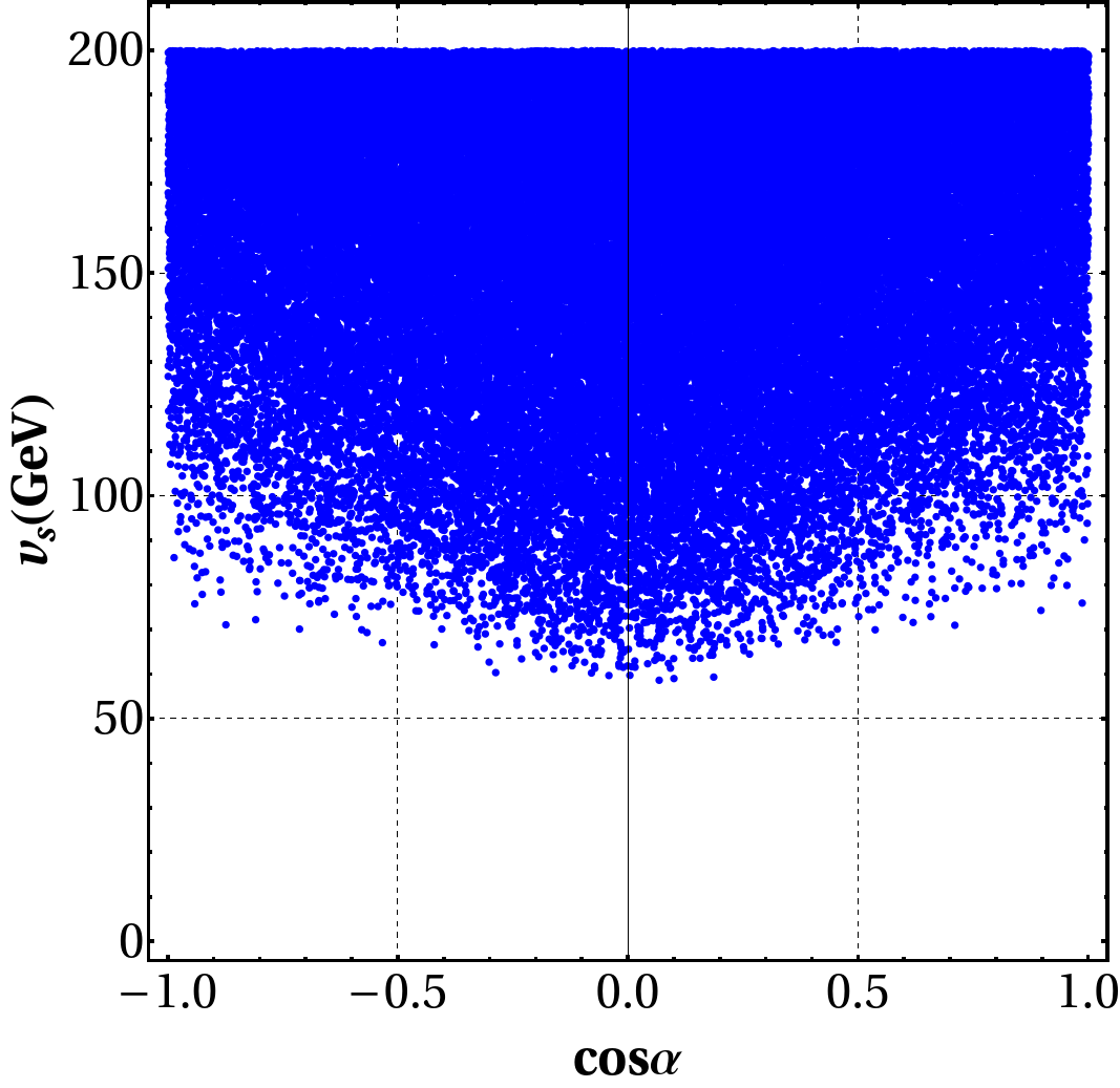
Figure 1: Parameter space in the $\cos\alpha-v_{s}$ plane. Blue points stand for these that satisfy all the theoretical constraints.

Experimental constraints

II.3.3 LHC Higgs boson data and its projections for future hadron colliders

To complement the theoretical constraints, we also analyze the experimental measurements from LHC and its projections for the HL-LHC and HE-LHC. For a decay $S\to X$ or a production process $\sigma(pp\to S)$, the signal strength is defined as

$$\mathcal{\mu}_{X}=\frac{\sigma(pp\to h)\cdot\mathcal{BR}(h\to X)}{\sigma(pp\to h^{\text{SM}})\cdot\mathcal{BR}(h^{\text{SM}}\to X)},$$ (13)

where $\sigma(pp\to S)$ is the production cross section of $S$, with $S=h,\,h^{\text{SM}}$; here $h$ is the SM-like Higgs boson coming from an extension of the SM and $h^{\text{SM}}$ is the SM Higgs boson; $\mathcal{BR}(S\to X)$ is the branching ratio of the decay $S\to X$, where $X=c\bar{c},\;b\bar{b},\;\tau^{-}\tau^{+},\;\mu^{-}\mu^{+},\;WW^{*},\;ZZ^{*},\;\gamma\gamma$. In our analysis of $\mu_{X}$, we consider $\tilde{Z}_{bb}=0.01$ and $\tilde{Z}_{tt}=0.4$. Such values are well motivated because they simultaneously accommodate all the $\mu_{X}$’s. In fact, values in the $0.01\leq\tilde{Z}_{bb}\leq 0.1$ and $0.1\leq\tilde{Z}_{tt}\leq 1$ intervals have no important impact on the $\mu_{X}$’s. However, in the case $\tilde{Z}_{bb}\geq 0.1$ and $\tilde{Z}_{tt}\geq 2$, a large reduction of allowed values in the $\cos\alpha-v_{s}$ plane is found.

II.3.4 Lepton Flavor-Violating processes

Furthermore, we also analyze lepton flavor-violating processes that can help us to complement the model parameter space in the $\cos\alpha-v_{s}$ plane. The processes considered for that aim are i) upper limits on the $\mathcal{BR}(\mu\to e\gamma)$, $\mathcal{BR}(\tau\to\mu\gamma)$, $\mathcal{BR}(\tau\to e\gamma)$, ii) upper limits on $\mathcal{BR}(\mu\to 3e)$, $\mathcal{BR}(\tau\to 3e)$, $\mathcal{BR}(\tau\to 3\mu)$ and $\mathcal{BR}(\mu\to\mu ee)$, iii) measurements of the $\mathcal{BR}(B_{s}\to\mu\mu)$ and $\mathcal{BR}(B_{d}\to\mu\mu)$ and finally iv) muon anomalous magnetic moment $\delta a_{\mu}$. The processes i)-iii) are not very restrictive in the FNSM. This is mainly because of the choice we made for the matrix elements $\tilde{Z}_{\mu\mu}$ and $\tilde{Z}_{\tau\tau}$, as they play a subtle role in the couplings (see Tab. 1) $\phi\mu\mu$ and $\phi\tau\tau$ $(\phi=h,\,H_{F},\,A_{F})$, which have a significant impact on the observables $\tau\to 3\mu$, $\tau\to\mu\gamma$, $\mu\to e\gamma$. In fact, we consider $\tilde{Z}_{\tau\tau}=0.2$ and $\tilde{Z}_{\mu\mu}=10^{-4}$ (hence, a strong hierarchy), otherwise the SM $h\mu\mu$ coupling would be swamped by corrections from the FNSM. In contrast, we find that the most stringent constraint comes from $\delta a_{\mu}$, which imposes an upper limit on the complex singlet VEV $v_{s}$. However, the situation could change because is still possible that more precise determinations of the SM hadronic contribution and the experimental measurement would settle the discrepancy in the future without requiring any new physics effects. Thus, in this work we remain conservative but with an open stance to the above described happening.

We present in Fig. 2 the most restrictive observables of the model parameter space, limitedly to the reduced intervals $-1\leq\cos\alpha\leq-0.95$ and $0.95\leq\cos\alpha\leq 1$ since it is the region in which all the analyzed observables converge.

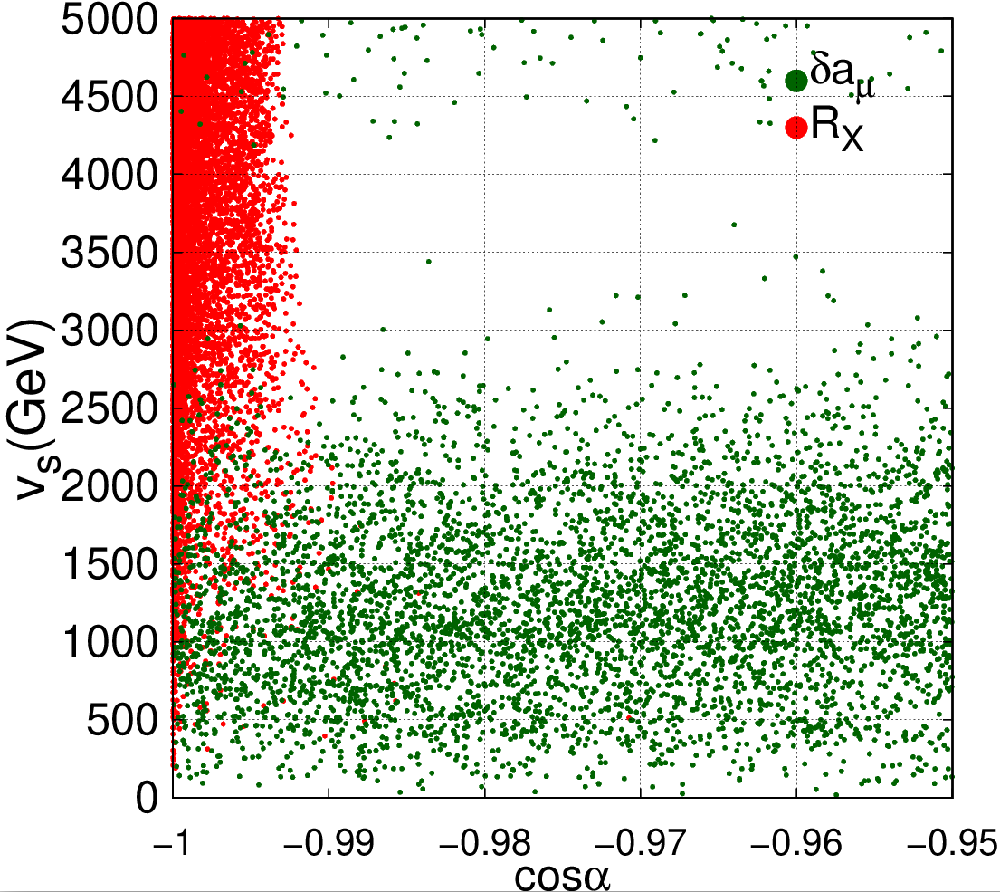
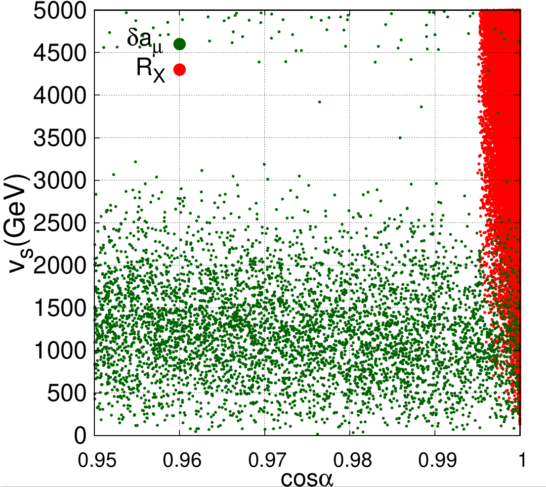
Figure 2: Allowed region by all the constraints studied in the $\cos\alpha-v_{s}$ plane. (a) Interval limited $-1\leq\cos\alpha\leq-0.95$ and (b) Interval limited $0.95\leq\cos\alpha\leq 1$. Red points correspond to those allowed by all the $\mu_{X}$’s, while the green points represent to those allowed by $\delta a_{\mu}$.

It is important to mention that quark flavor constraints, namely, $B-\bar{B}$ mixing, $K-\bar{K}$ mixing and $D-\bar{D}$ mixing might impose severe restrictions on some model parameters. In Ref. Abbas:2024dfh ; Bauer:2016rxs this is made evident on the $M_{A_{F}}-v_{s}$ plane, which strictly bounds $M_{A_{F}}$ as a function of $v_{s}$. We avoid these dangerous bounds via the deletion of the matrix elements $\tilde{Z}_{db}$, $\tilde{Z}_{ds}$ and $\tilde{Z}_{uc}$ (see Table 1) for $B-\bar{B}$ mixing, $K-\bar{K}$ mixing, $D-\bar{D}$ mixing, respectively. To make this clear, we present in Fig. 3 the $M_{H_{F}}-v_{s}$ plane for three different values of $\tilde{Z}_{uc}$; $10^{-10}$, $10^{-9}$ and $5\times 10^{-9}$. The colored areas are these allowed by $|M_{12}^{D}|$ Bevan:2014tha .

$$|M^{D}_{12}|<7.5\times 10^{-3}~\text{ps}^{-1}\;.$$ (14)

Similar constraints are obtained for $K-\bar{K}$ and $B-\bar{B}$.

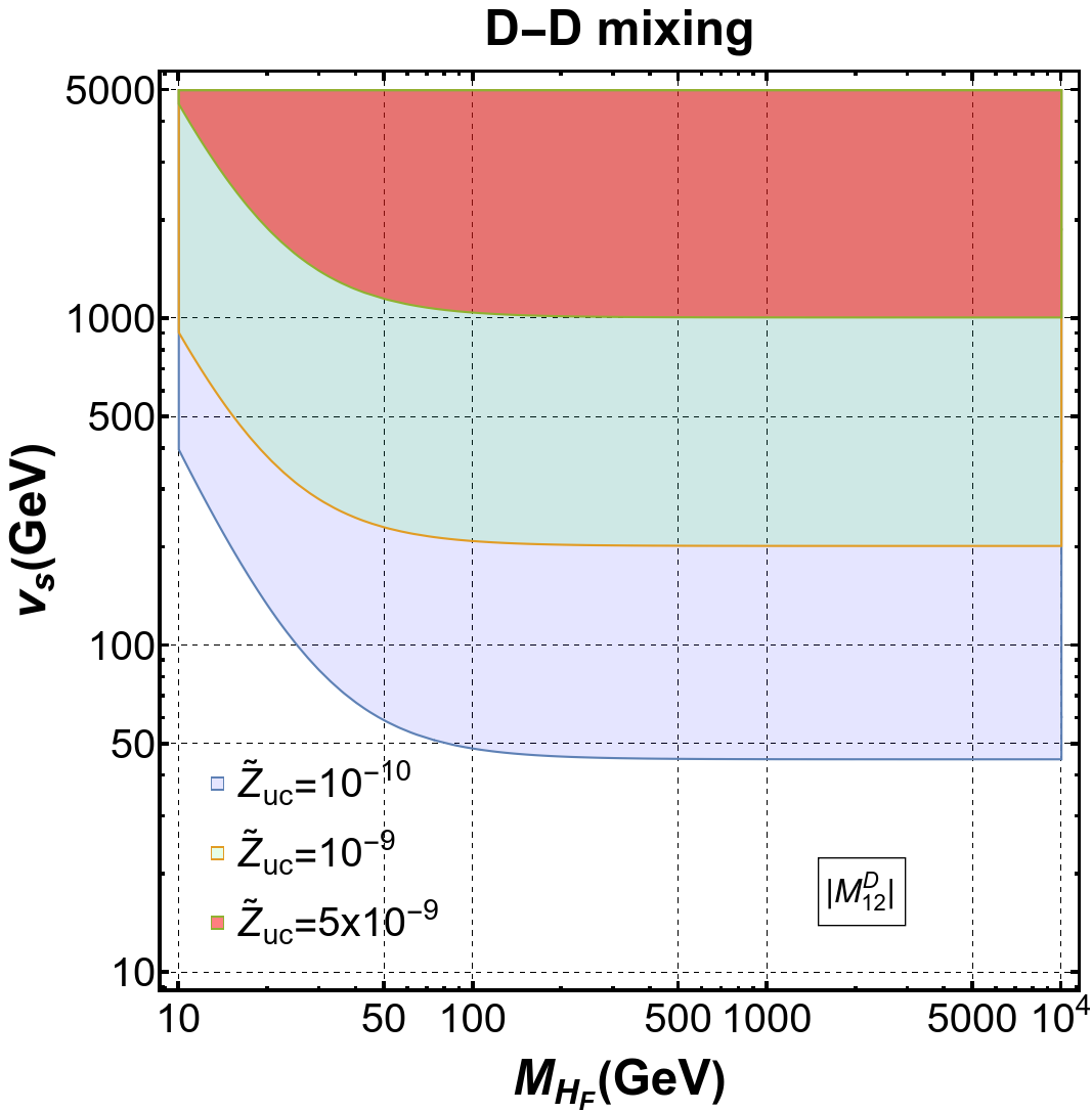
Figure 3: $M_{H_{F}}-v_{s}$ plane showing the region allowed due to flavon contributions to $|M_{12}^{D}|$. Blue area: $\tilde{Z}_{uc}$=$10^{-10}$, green area: $\tilde{Z}_{uc}$=$10^{-9}$, red area: $\tilde{Z}_{uc}$=$5\times 10^{-9}$.

In conclusion, we define four benchmark points (BMP) to be used in the simulations in the next section.

• BMP1: $v_{s}=301$ GeV, $\cos\alpha=0.998$,

• BMP2: $v_{s}=353$ GeV, $\cos\alpha=-0.997$,

• BMP3: $v_{s}=888$ GeV, $\cos\alpha=-0.999$,

• BMP4: $v_{s}=191$ GeV, $\cos\alpha=-0.999$.

III Collider analysis

This section presents a compressive study on the signal and SM background processes. We also present the strategy for separating one from the other. Explicit analytic expressions for the production mechanism of the flavon and its decay into photons are also presented.

Production and decay of the flavon

We are interested in the production of the CP-even flavon $H_{F}$, the dominant mechanism for producing it is via gluon fusion. This interaction can be extracted through the Lagrangian:

$$\mathcal{L}_{\rm eff} = \frac{1}{v}\,g_{hgg}\,h\,G_{\mu\nu}G^{\mu\nu},$$ (15)

$$g_{Sgg} = -i\,\frac{\alpha_{S}}{8\pi}\,\tau(1+(1-\tau)\,f(\tau))~~~~~{\rm with}~~\tau=\frac{4M_{t}^{2}}{M_{h}^{2}},$$ (16)

$$f(\tau) = \begin{cases}(\sin^{-1}\sqrt{\frac{1}{\tau}})^{2},\quad\quad\quad\quad\quad\quad\tau\geq 1,\\ -\frac{1}{4}[\ln\frac{1+\sqrt{1-\tau}}{1-\sqrt{1-\tau}}-i\pi]^{2}\quad\quad\quad\tau<1.\end{cases}$$ (17)

In FNSM, the $ggh$, $ggH_{F}$ and $ggA_{F}$ couplings are given, respectively, by:

$$g_{hgg}=\left(\frac{c_{\alpha}v_{s}-s_{\alpha}v}{v_{s}}\right)g_{Sgg}$$ (18)

$$g_{H_{F}gg}=\left(\frac{c_{\alpha}v+s_{\alpha}v_{s}}{v_{s}}\right)g_{Sgg}$$ (19)

$$g_{A_{F}gg}=\frac{v}{v_{s}}\,(-i\,\alpha_{S}/\pi)\,\tau\,f(\tau)$$ (20)

We present in Fig. 4 the production cross section of the flavon $H_{F}$ as a function of its mass for the colliders: HL-LHC ($\sqrt{s}=14$ TeV), HE-LHC ($\sqrt{s}=27$ TeV), FCC-hh ($\sqrt{s}=100$ TeV), and the BMPs defined in Sec. II.3.4.

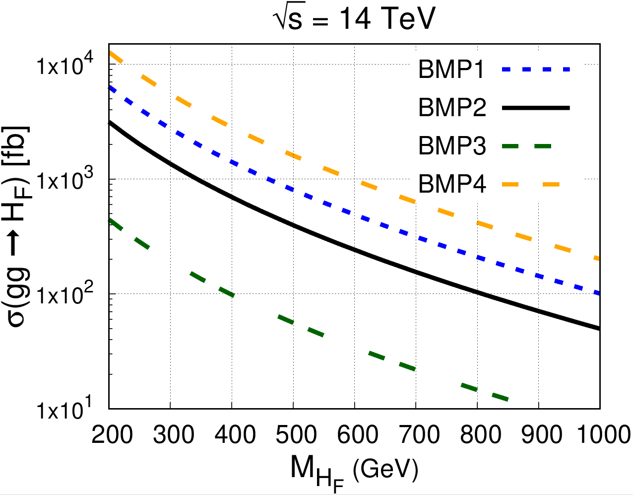
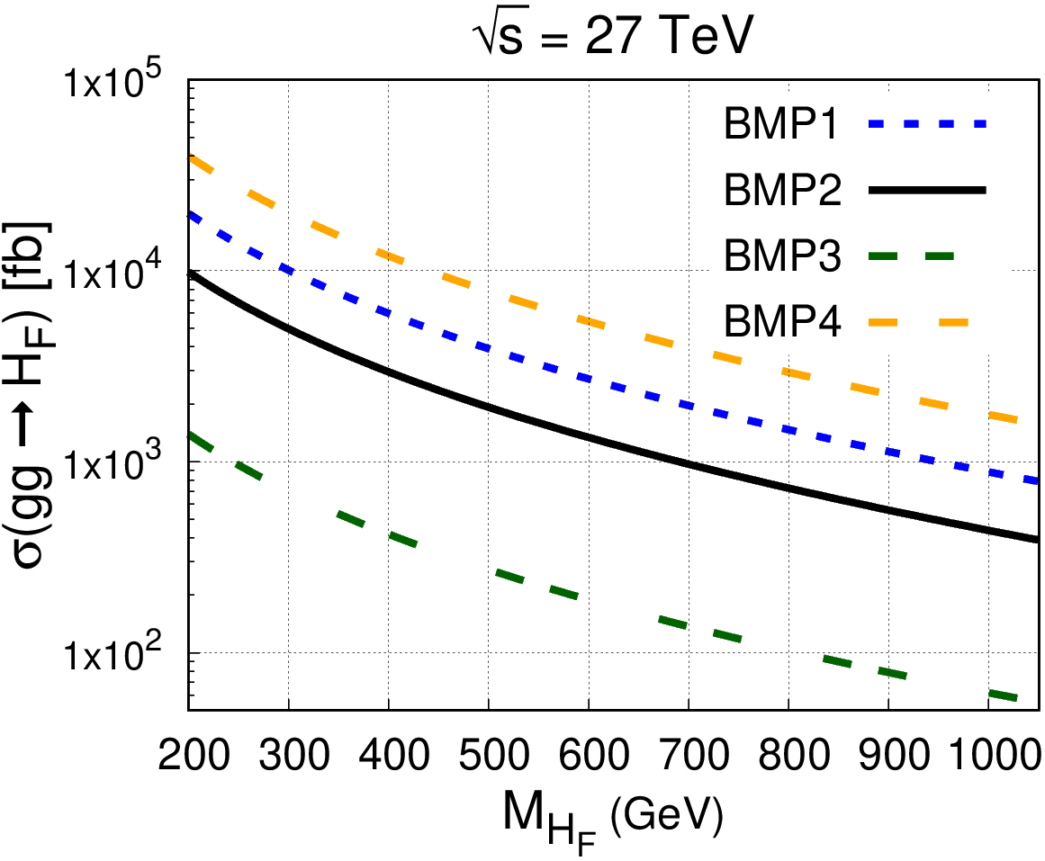
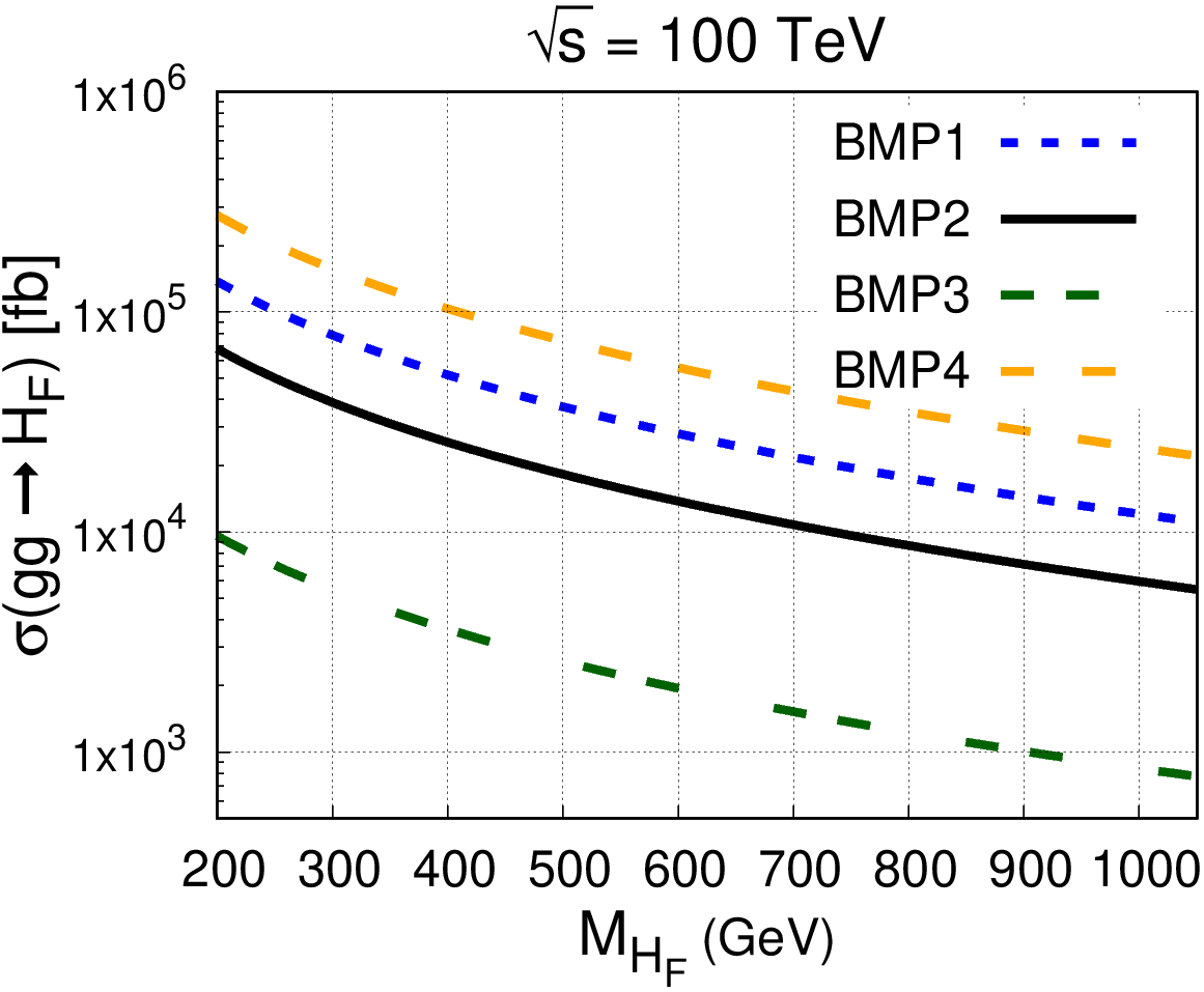
Figure 4: Production cross-section of the flavon via gluon fusion in $pp$ collisions $\sigma(gg\to H_{F})$. (a) For the HL-LHC at $\sqrt{s}=14$ TeV, (b) For the HE-LHC at $\sqrt{s}=27$ TeV, (a) For the FCC-hh at $\sqrt{s}=100$ TeV.

The most optimistic case for producing flavons is BMP4, which predicts cross sections (at $\sqrt{s}=14$ TeV), from $200$ to $10^{4}$ fb, corresponding to the range of masses $200-1000$ GeV. In contrast, the least favored scenario is BMP3. The cross section of this scenario range from $8$ fb to $500$ fb for $M_{H_{F}}=1000,\,200$, respectively. These values are expected because the singlet complex VEV $v_{s}$ suppresses the FNSM correction of the flavon production via gluon fusion, as shown in Eq. (19). For $\sqrt{s}=27,\,100$ TeV, the cross sections are up to 1 and 2 orders of magnitude larger than 14 TeV, respectively.

On the other hand, we also need to know the branching ratio of the decay $H_{F}\to\gamma\gamma$, which can be obtained with the following expression:

$$\Gamma(H_{F}\to\gamma\gamma)=\frac{\alpha^{2}M_{H_{F}}^{3}}{1024\pi^{3}m_{W}^{2}}\Bigg{|}\sum_{s}A_{s}^{H_{F}\gamma\gamma}(\tau_{s})\Bigg{|}^{2},$$ (21)

where the subscript $s=0,1/2,1$ refers to the spin of the charged particle circulating in the loop, and

$$A_{s}^{H_{F}\gamma\gamma}=\begin{cases}\displaystyle{\sum_{f}\frac{2m_{W}g_{H_{F}f_{i}\bar{f}_{i}}N_{c}Q_{f}^{2}}{m_{f}}\Big{[}-2\tau_{s}\big{(}1+(1-\tau_{s})f(\tau_{s})\big{)}\Big{]}}&{\rm for~}s=\frac{1}{2},\\ \displaystyle{g_{H_{F}WW}\Big{[}2+3\tau_{W}+3\tau_{W}(2-\tau_{W})f(\tau_{W})\Big{]}}&{\rm for~}s=1,\\ \end{cases}$$ (22)

where

$$f(x)=\begin{cases}\displaystyle{\arcsin^{2}\Bigg{(}\frac{1}{\sqrt{x}}\Bigg{)},}&x\geq 1,\\ \displaystyle{-\frac{1}{4}\Bigg{[}\log\Bigg{(}\frac{1+\sqrt{1-x}}{1-\sqrt{1-x}}\Bigg{)}-i\pi\Bigg{]}^{2}},&x<1.\end{cases}$$ (23)

and $N_{c}=1,3$ for leptons and quarks, respectively, $\tau_{a}=4M_{a}^{2}/M_{H_{F}}^{2}$. The couplings $g_{H_{F}f_{i}\bar{f}_{i}}$ and $g_{H_{F}WW}$ are given in Table 1. Figure 5 shows the $\mathcal{BR}(H_{F}\to\gamma\gamma)$ as a function of the flavon mass $M_{H_{F}}$ for the BMPs defined in Sec. II.3.4.

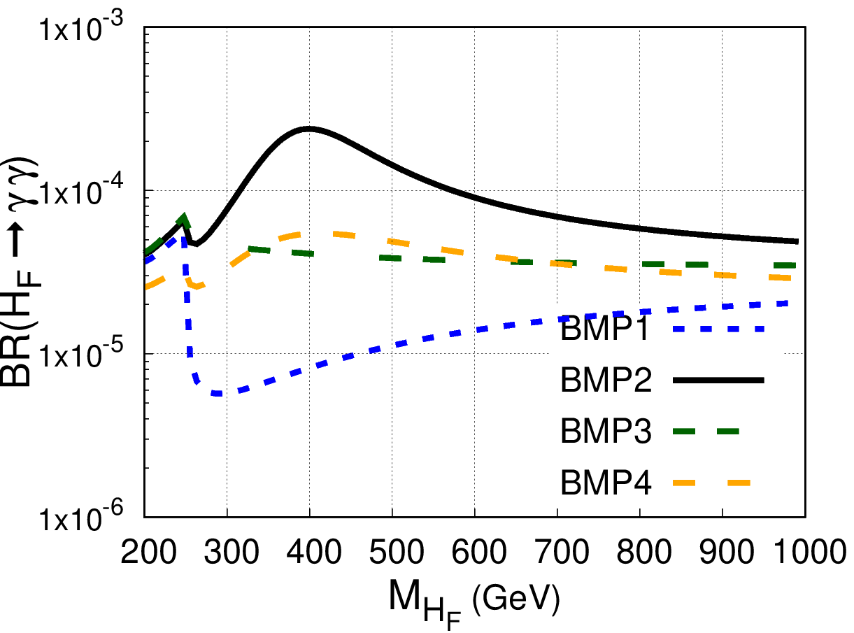
Figure 5: Branching ratio $\mathcal{BR}(H_{F}\to\gamma\gamma)$ as a function of the Flavon mass $M_{H_{F}}$.

According to our analysis of the FNSM parameter space, branching ratios from $\mathcal{O}(10^{-6})$ to $\mathcal{O}(10^{-4})$ can be obtained, for BMP2 ($M_{H_{F}}\sim 400$ GeV) and BMP1 ($M_{H_{F}}\sim 250$ GeV), respectively; while for BMP3 and BMP4 we obtain similar branching ratios for the range $320\leq M_{H_{F}}\leq 1000$ GeV. The discontinuous behavior in all BMPs is due to several factors, the most distinctive being the emergence or suppression of different flavon decay channels. In particular, once $M_{H_{F}}\sim 250$ GeV, there is an inflection point associated with the emergence of the $H_{F}\to hh$ di-Higgs channel. For $M_{H_{F}}>1000$ GeV, the $\mathcal{BR}(H_{F}\to\gamma\gamma)$ converges to a value of order $10^{-5}$. The values of the branching ratios are relatively high due to the BMPs defined for our study. From Eq. (22) and Table 1, we notice that $\mathcal{BR}(H_{F}\to\gamma\gamma)\sim 1/v_{s}$, with $v_{s}$ being of order $10^{2}$ in the BMPs defined, it suppresses the $\mathcal{BR}(H_{F}\to\gamma\gamma)$ by a factor of $10^{-2}$ with respect to the $\mathcal{BR}(h\to\gamma\gamma)$ of the SM, which is of order $10^{-3}$. Thus, the $\mathcal{BR}(H_{F}\to\gamma\gamma)$ shown in Fig. 5 are reasonable and motivate their possible experimental scrutiny.

Signal and background

• Signal: We search for a final state $\gamma\gamma$ generated by the decay $H_{F}\to\gamma\gamma$, where the flavon $H_{F}$ is produced by gluon fusion. The analysis is performed in the mass range of 200-1000 GeV. We present in Fig. 6 the Feynman diagram of the signal. While Fig. 7 shows the production cross section $\sigma(gg\to H_{F}\to\gamma\gamma)$ (left vertical axis) and the number of events produced (right vertical axis) as a function of $M_{H_{F}}$.

  

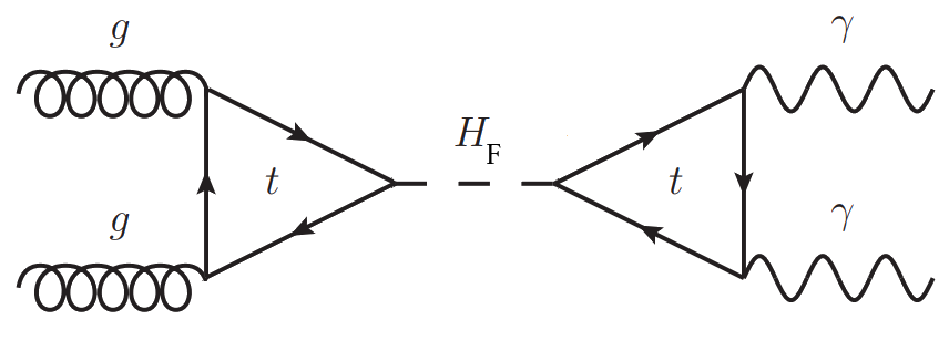
  Figure 6: Feynman diagram of the signal $gg\to H_{F}\to\gamma\gamma$.

  

  

  

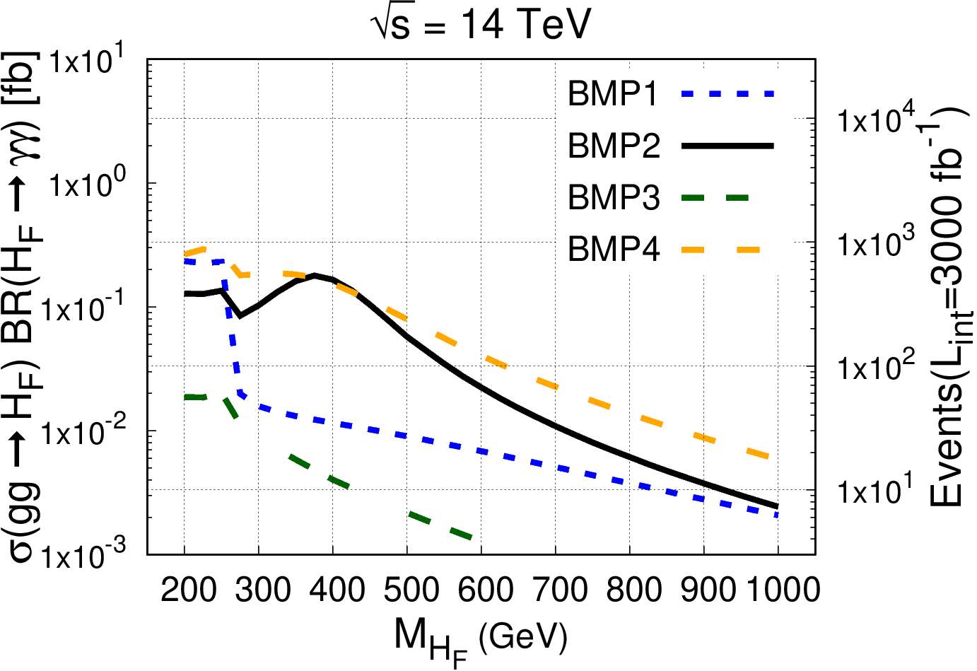
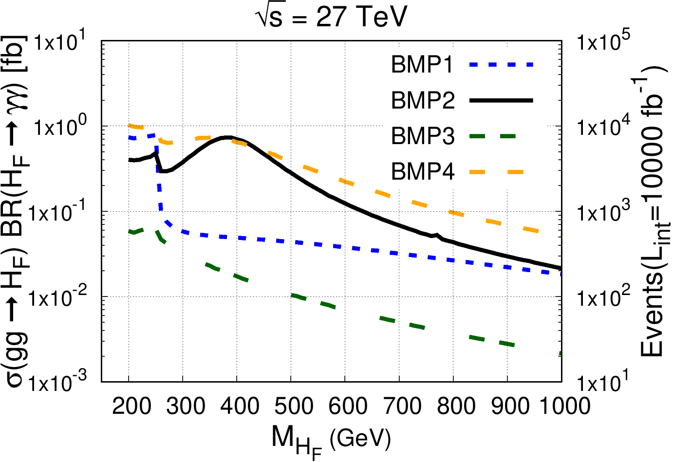
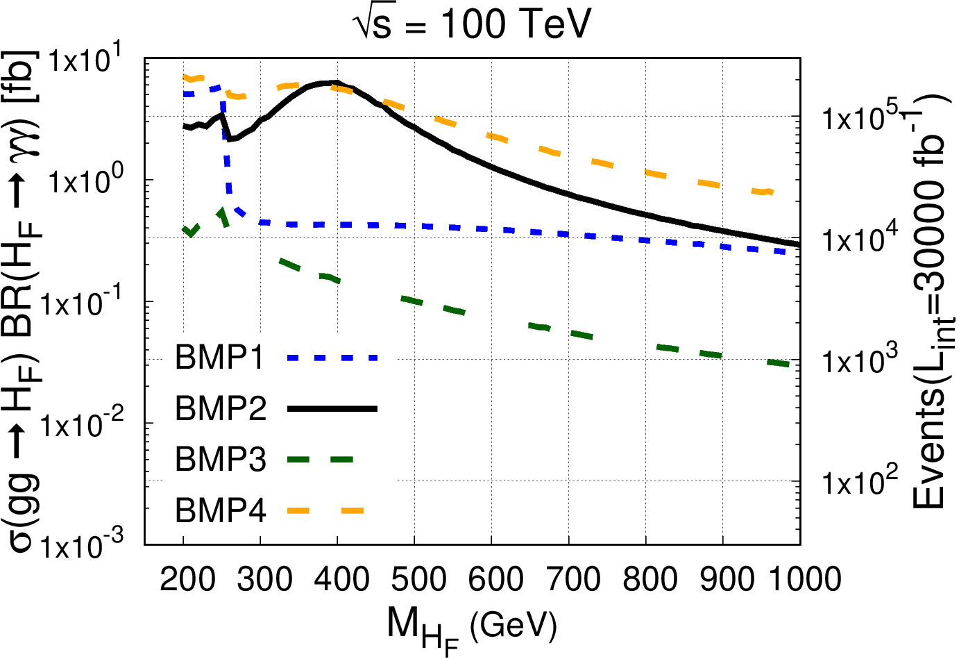
  Figure 7: On the left vertical axis: Production cross-section $\sigma(pp\to H_{F}\to\gamma\gamma)$ as a function of the Flavon mass $M_{H_{F}}$. On the right vertical axis: Number of events produced as a function of the Flavon mass $M_{H_{F}}$.

• Background: The dominant irreducible background is the SM di-photon production ($\gamma\gamma$); contributions also come from $\gamma+j$ and $j+j$ production with one or two jets misidentified as photons and from the Drell-Yan process.

Event selection

The identification of the signal depends mainly on the true $p_{T}^{\gamma}$ of the photons. The photon selection efficiency as a function of the $p_{T}^{\gamma}$ of the true photon is parametrised by

$$\epsilon(p_{T}^{\gamma})=0.76-1.98\times e^{-\frac{p_{T}^{\gamma}}{16.1\rm GeV}}.$$ (24)

On the other hand, the rate of jets passing the photon identification and isolation requirements can be identified as fake photons. The rate is parametrised as a function of the true jet $p_{T}^{j}$ via :

$$\epsilon(p_{T}^{j})=9.3\cdot 10^{-3}\times e^{-\frac{p_{T}^{j}}{27.5\rm GeV}}.$$ (25)

The strategy to isolate the signal from the background is to impose the criteria in Eqs. (24)-(25) and to perform a Boosted Decision Trees (BDT) training Book:bdt by using variables related to the kinematics of the final state. Table 3 shows the variables used to train and test the signal and background events.

Table 3: List of the variables used to train and test the signal and background events.

Rank	Variable	Description
1	$p_{T}^{\gamma_{1}}$	Photon with the largest transverse momentum.
2	$M_{{\rm inv}}(\gamma\gamma)$	Invariant mass
3	$N(j)$	Number of jets
4	$\Delta R$	The $R$ separation between the photons
5	$p_{T}^{\gamma_{2}}$	Tranverse momentum of the subleading photon
6	$\eta_{1}$	Pseudorapidity of the leading photon
7	$\eta_{2}$	Pseudorapidity of the subleading photon
8	$\phi(\gamma_{1})$	Azimuth angle of the leading photon
9	$\phi(\gamma_{2})$	Azimuth angle of the subleading photon

According to our analysis, the most discriminating observables are the transverse momentum of the leading photon $p_{T}^{\gamma_{1}}$ and the invariant mass $M_{\rm inv}(\gamma\gamma)$. We show in Fig. 8 these distributions for $M_{H_{F}}=400$ GeV.

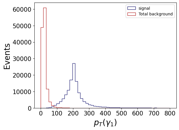
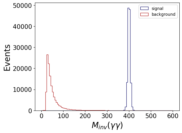
Figure 8: (a) Transverse momentum of the leading photon $p_{T}^{\gamma_{1}}$, (b) Invariant mass $M_{\rm inv}(\gamma\gamma)$ for $M_{H_{F}}=400$ GeV.

Meanwhile, Fig. 9 presents the discriminant for the signal and background.

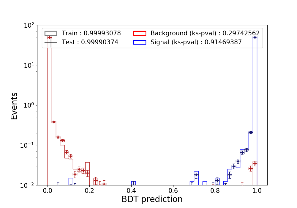
Figure 9: Plot of the discriminant for signal and background data.

The goodness of fit is checked via the Kolmogorov-Smirnov (KS) test. Our analysis shows that the KS value is within the permissible $[0,\,1]$ interval, namely, 0.29 and 0.91 for the background and the signal, respectively. The relevant hyperparameters for the BDT training are as follows: Number of trees NTree=110, maximum depth of the decision tree MaxDepth=4, maximum number of leaves MaxLeaves=14. The training is performed using the MC-simulated samples. These signal and background samples are scaled to the expected number of candidates, which is calculated based on the integrated luminosity and cross sections. The BDT selection is optimized individually for each flavon mass $M_{H_{F}}$ to maximize the figure of merit, i.e., the signal significance, defined as $S/\sqrt{S+B}$, where $S$ and $B$ represent the number of signal and background candidates, respectively, in the signal region after applying the selection criteria.

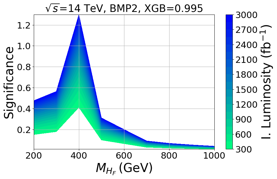
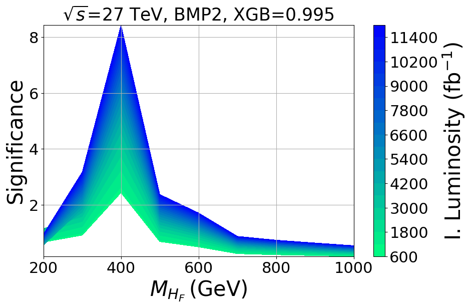
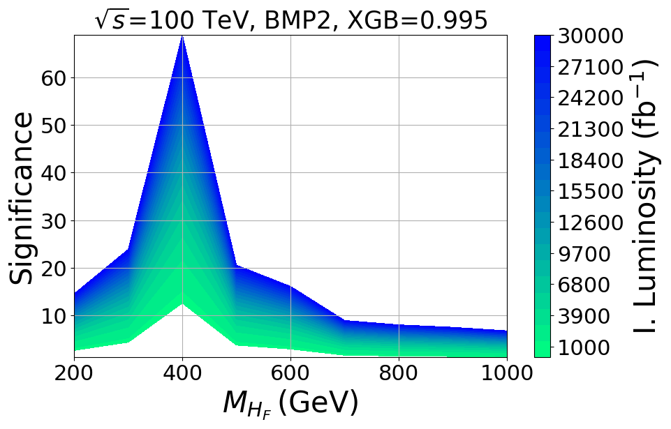
Figure 10: Significance as a function of the flavon mass $M_{H_{F}}$ and the integrated luminosity, for the BMP2. (a) HL-LHC, (b) HE-LHC and (c) FCC-hh. In all the cases we impose a cut on the BDT prediction XGB=0.995.

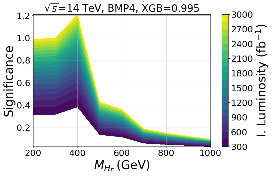
Figure 11: Significance as a function of the flavon mass $M_{H_{F}}$ and the integrated luminosity, for the BMP4. (a) HL-LHC, (b) HE-LHC and (c) FCC-hh. In all the cases we impose a cut on the BDT prediction XGB=0.995.

Figure 10 presents contour plots of the the signal significance as a function of the flavon mass $M_{H_{F}}$ and the integrated luminosity for the BMP2. In particular, we obtain signal significances at the level of $5\sigma$ for $350\lesssim M_{H_{F}}\lesssim 450$ GeV and $200\leq M_{H_{F}}\leq 1000$ GeV for the HE-LHC and FCC-hh, respectively. The least favored scenario is for the HL-LHC, which does not provide the ease of detection of the flavon. Similarly, Fig 11 presents the signal significance for the benchmark point BMP4 with similar results for the HL-LHC. However, this scenario provides a range of masses that could be detected slightly greater than the previous case. Specifically, the HE-LHC offers the possibility of detection of the flavon in the range of masses $200-450$ GeV. More encouraging results appear at FCC-hh, achieving a potential discovery in a wider range of masses, covering the entire mass spectrum studied in this paper. In contrast, for the least hopeful case, BMP3, we found a maximum significance of $2.12\sigma$ for the FCC-hh by considering its final integrated luminosity and $M_{H_{F}}=200$ GeV. As far as BMP1 is concerned, we find results that approach an intermediate case of BMPs 2 and 3 for $400\lesssim M_{H_{F}}\lesssim 600$ GeV and significances similar to BMP2 for $750\lesssim M_{H_{F}}\lesssim 1000$. The most relevant signal significances for the BMP1, even at the level of the most optimistic BMPs (2 and 4), lie in the mass interval $200\leq M_{H_{F}}\leq 250$.

IV Conclusions

In this paper, we have studied the production of the so-called flavon $H_{F}$, with its subsequent decay into two photons (signal). The flavon is a hypothetical particle predicted in a model that invokes the Froggatt-Nielsen mechanism, which is the theoretical framework considered in this paper. The mechanism of production of the flavon is via proton-proton collisions at super hadron colliders, namely: High-Luminosity LHC, High-Energy LHC and the Future hadron-hadron Circular Collider. To give realistic predictions, we test the free parameters of the model against theoretical and experimental constraints and then we define benchmark points (BMPs) to perform Monte Carlo simulations. The most severe constraint on the cosine of the mixing angle ($\cos\alpha\sim-1\,\text{or}\,\sim 1$) that mixes the neutral and real parts of the Higgs doublet and the complex singlet with the physical fields $h$ and $H_{F}$ comes from the LHC Higgs boson data and their projections for the HE-LHC. This is expected in order to avoid dangerous corrections to the Higgs boson couplings to fermions and gauge bosons. As far as the VEV of the complex singlet $v_{s}$ is concerned, the muon anomalous magnetic moment is the most restrictive observable on $v_{s}$, allowing $v_{s}\lesssim 3$ TeV. However, the situation could change because it is still possible that more precise determinations of the SM hadronic contribution and the experimental measurement would settle the discrepancy in the future without requiring any new physics effects. Thus, in this work we remain conservative but with an open stance to the above described happening.

On the other hand, based on the defined BMPs, and using events simulated for the signal and its SM background, we perform an analysis with machine learning via the Boosted Decision Trees method to isolate the signal from the background. We find that the nearest evidence could emerge at the HE-LHC with a signal significance of $5\sigma$ for integrated luminosities in the range $5-12$ ab^-1 and flavon masses between $350-450$ GeV ($200-450$) for the BMP2 (BMP4). These predictions could be corroborated in the Future hadron-hadron Circular Collider. Furthermore, this collider would have the capability to search for broader range of masses, covering the entire interval studied in this work. Thus, we predict signal significances at the level of $5\sigma$ for the range $200\leq M_{H_{F}}\leq 1000$ GeV. Even more, projecting our results, the FCC-hh might be able to search for flavon masses as high as 5 TeV.

References

- [1] S. L. Glashow. Partial Symmetries of Weak Interactions. Nucl. Phys., 22:579–588, 1961.
- [2] Steven Weinberg. A Model of Leptons. Phys. Rev. Lett., 19:1264–1266, 1967.
- [3] Abdus Salam and John Clive Ward. Weak and electromagnetic interactions. Nuovo Cim., 11:568–577, 1959.
- [4] Gerard ’t Hooft and M. J. G. Veltman. Regularization and Renormalization of Gauge Fields. Nucl. Phys. B, 44:189–213, 1972.
- [5] T. W. B. Kibble. Symmetry breaking in nonAbelian gauge theories. Phys. Rev., 155:1554–1561, 1967.
- [6] Peter W. Higgs. Broken Symmetries and the Masses of Gauge Bosons. Phys. Rev. Lett., 13:508–509, 1964.
- [7] Peter W. Higgs. Spontaneous Symmetry Breakdown without Massless Bosons. Phys. Rev., 145:1156–1163, 1966.
- [8] G. S. Guralnik, C. R. Hagen, and T. W. B. Kibble. Global Conservation Laws and Massless Particles. Phys. Rev. Lett., 13:585–587, 1964.
- [9] Peter W. Higgs. Broken symmetries, massless particles and gauge fields. Phys. Lett., 12:132–133, 1964.
- [10] F. Englert and R. Brout. Broken Symmetry and the Mass of Gauge Vector Mesons. Phys. Rev. Lett., 13:321–323, 1964.
- [11] Georges Aad et al. Observation of a new particle in the search for the Standard Model Higgs boson with the ATLAS detector at the LHC. Phys. Lett., B716:1–29, 2012.
- [12] Serguei Chatrchyan et al. Observation of a new boson with mass near 125 GeV in pp collisions at = 7 and 8 TeV. JHEP, 06:081, 2013.
- [13] C. D. Froggatt and Holger Bech Nielsen. Hierarchy of Quark Masses, Cabibbo Angles and CP Violation. Nucl. Phys. B, 147:277–298, 1979.
- [14] M. A. Arroyo-Ureña, J. L. Díaz-Cruz, G. Tavares-Velasco, A. Bolaños, and G. Hernández-Tomé. Searching for lepton flavor violating flavon decays at hadron colliders. Phys. Rev. D, 98(1):015008, 2018.
- [15] Marco A. Arroyo-Ureña, Amit Chakraborty, J. Lorenzo Díaz-Cruz, Dilip Kumar Ghosh, Najimuddin Khan, and Stefano Moretti. Flavon signatures at the HL-LHC. Phys. Rev. D, 108(9):095026, 2023.
- [16] Gauhar Abbas, Ashutosh Kumar Alok, Neetu Raj Singh Chundawat, Najimuddin Khan, and Neelam Singh. Finding flavons at colliders. Phys. Rev. D, 110(11):115015, 2024.
- [17] Amit Chakraborty, Dilip Kumar Ghosh, Najimuddin Khan, and Stefano Moretti. Exploring the Dark Sector of the inspired FNSM at the LHC. 5 2024.
- [18] G. Apollinari, O. Brüning, T. Nakamoto, and Lucio Rossi. High Luminosity Large Hadron Collider HL-LHC. CERN Yellow Rep., (5):1–19, 2015.
- [19] Michael Benedikt and Frank Zimmermann. Proton Colliders at the Energy Frontier. Nucl. Instrum. Meth. A, 907:200–208, 2018.
- [20] Nima Arkani-Hamed, Tao Han, Michelangelo Mangano, and Lian-Tao Wang. Physics opportunities of a 100 TeV proton–proton collider. Phys. Rept., 652:1–49, 2016.
- [21] Najimuddin Khan and Subhendu Rakshit. Study of electroweak vacuum metastability with a singlet scalar dark matter. Phys. Rev. D, 90(11):113008, 2014.
- [22] Martin Bauer, Torben Schell, and Tilman Plehn. Hunting the Flavon. Phys. Rev. D, 94(5):056003, 2016.
- [23] A. J. Bevan et al. The utfit collaboration average of d meson mixing data: Winter 2014. JHEP, 1403:123, 2014.
- [24] L. Breiman et al. Classification and regression trees. Wadsworth international group, California, USA, 1984.