The principle of simultaneous saturation: applications to multilinear models for the restriction and Bochner-Riesz problem

Abstract.

We introduce a new technique for the fields of harmonic analysis and PDE, simultaneous saturation. Simultaneous saturation is a framework for controlling the size of a set where each element of the set is large. In this paper we apply this framework to multilinear restriction type estimates. Here the elements of the set are $Tf(p)$ where $T$ is an multilinear oscillatory integral operator. Controlling the size of the set where $Tf(p)$ is large allows us to obtain efficient $L^{p}$ estimates for the operator $T$. From this perspective we produce a new and independent of Bennett-Carbery-Tao [2] proof of the multilinear restriction theorem. Further we then establish new results on multilinear models for the Bochner-Riesz problem that allow parameter dependent degeneration of the transversality condition.

As an analyst one is frequently faced with the problem of controlling the size of objects or sets of objects. For example to study the $L^{q}(X)\to L^{p}(Y)$ mapping norms of an operator $T:L^{q}(X)\to L^{p}(Y)$ we need to control the size of the set of points $\{Tf(p)\mid p\in Y,f\in L^{q}(X)\}$. Often it is reasonable tractable to find a sharp supremum bound that controls how large an individual point can be. We say that an estimate is sharp if we can find some example that saturates it. That is if we have a supremum bound, $|Tf(\cdot)|\leq K$, then we can find a saturating example by finding a function $f$ and a point $p$ so that $|Tf(p)|=K$ (where we are looking at a parameter dependent problem we often also understand saturation as $|Tf(p)|\geq{}cK$ for a universal constant $c$). Of course there can be many such pairs $(f,p)$ and usually there is an interdependence between the function $f$ and point $p$. To gain a more sophisticated understanding of the size set $\{Tf(p)\mid(f,p)\text{ saturates }\}$ we need to understand where we can simultaneously saturate at more than one point. To do this we need a number of points $\{p_{1},\dots,p_{N}\}$ and one function $f$ so that $|Tf(p_{j})|=K$ for any $j$.

Of course if $Tf(p)$ simultaneously saturates at all the points then any average of $\{Tf(p_{1}),\dots,Tf(p_{N})\}$ must also saturate the $L^{\infty}$ bounds. But what sort of average should we use? The simplest is a arithmetic average, ie

$$\frac{1}{N}\sum_{j=1}^{N}\alpha_{j}Tf(p_{j})\quad|\alpha_{j}|=1.$$

One might then try to show that the average must be smaller than the saturation bound (for instance due to some kind of cancellation between terms). This is however not an ideal way to work with averages. First, if some of the $Tf(p_{j})$ are large but others are very small the average might still be large. So arithmetic averages are not sensitive enough to small data. Also exploiting cancellations in sums is generally a very difficult problem in itself.

Instead we propose studying geometric averages. That is we consider the product

$$\left(\prod_{j=1}^{N}|Tf(p_{j})|\right)^{1/N}.$$

Geometric averages are much more sensitive to small data points. If we can find upper bounds on the product (other than the trivial one) we can rule out simultaneous saturation on this collection of points. In this paper we will consider the $T:L^{q}(X)\to L^{p}(Y)$ mapping problem for $T$ an oscillatory integral operator

(1) $$Tf=\int e^{i\lambda\phi(x,\xi)}f(\xi)d\xi\quad\lambda\to\infty$$

by taking geometric averages $N$ points $p_{j}$ where $Tf(p_{j})\approx K(\lambda)$. Operators of the form (1) are intensely studied in the fields of harmonic analysis and PDE. See for example the texts [4] and [5].

The key idea is that we want to create some kind of barrier to there being a large number of points, that is we need to find an upper bound on $N$. We will take a product

(2) $$\prod_{j=1}^{N}Tf(p_{j})$$

and see this as the operator

$$\boldsymbol{T}=\underbrace{T\otimes\cdots\otimes T}_{N\text{ times }}\text{ acting on }\boldsymbol{F}=\underbrace{f\otimes\cdots\otimes f}_{N\text{ times}}$$

evaluated at the point $P=(p_{1},\dots,p_{N})$. Therefore we need to work in a high-dimensional space, one dimension for each of the $p_{j}$. Now, because (2) is a product, we can, of course, permute the order of the $p_{j}$. Accordingly we construct a finite dimensional measure space based on point measures supported at permutations of $(p_{1},\dots,p_{N})$, $P_{\sigma}=(p_{\sigma(1)},\dots,p_{\sigma(N)})$.

Within this framework, we need to record whether two pairs of points can be made simultaneously large. This is achieved with an energy matrix. The $(\sigma,\tau)$ entry of the energy matrix gives us information about whether $\boldsymbol{T}\boldsymbol{F}$ can be simultaneously large at $P_{\sigma}$ and $P_{\tau}$. In this paper we construct the energy matrix from $\boldsymbol{T}\boldsymbol{T}^{\star}$. From the energy matrix, we will show that if N is too large, we would be able to create some illegal ensembles. The ensembles are created by considering paths through the matrix. For instance we might connect $P_{\sigma_{1}}$ to $P_{\sigma_{100}}$ (the $(\sigma_{1},\sigma_{100})$ entry of the matrix tells us if this is possible) then $P_{\sigma_{100}}$ to $P_{\sigma_{54}}$ (the $(\sigma_{100},\sigma_{54})$ entry of the matrix determines whether this connection is possible). If both connections are possible we have an ensemble

$$P_{\sigma_{1}}\xleftrightarrow{}P_{\sigma_{100}}\xleftrightarrow{}P_{\sigma_{54}}$$

For this ensemble to be possible we require that both the $(\sigma_{1},\sigma_{100})$ and the $(\sigma_{100},\sigma_{54})$ entries of the matrix be large. The illegality of an ensemble arises from the properties of the operator $T$ and the points appearing in the ensemble.

In this paper the illegal ensembles will be loops of points that are illegal due to geometric constraints. At this point it is helpful to specialise to a particular example to fully demonstrate the technique. Suppose for example we consider (as we will do in Section 2) the multilinear restriction problem. This problem is closely related to the celebrated Fourier restriction/extension problem, see [1] for a good discussion of the relationship. While the Fourier restriction/extension problem is stated in terms of curvature, the multilinear restriction problem is about transversality. In this problem we consider the multilinear operator

$$\prod_{m=1}^{d}T_{m}f_{m}\quad f_{m}\in L^{2}(H_{m})$$

where

$$T_{m}f(x)=\int_{H_{m}}e^{i\lambda\langle x,\xi\rangle}f(\xi)d\mu_{m}(\xi)\quad x\in\mathbb{R}^{d}$$

where $H_{m}\subset\mathbb{R}^{d}$ is a hypersurface and $\mu_{m}$ its hypersurface measure. The set of hypersurfaces $\{H_{m}\}$ are assumed to have normals $\nu_{m}$ so that

$$|\nu_{1}\wedge\cdots\wedge\nu_{d}(x)|\geq{}C.$$

Since we are studying a multilinear problem, we want to estimate

$$\left|\!\left|{\prod_{m=1}^{d}T_{m}f_{m}}\right|\!\right|_{L^{p/d}}$$

in terms of

$$\prod_{m=1}^{d}\left|\!\left|{f}\right|\!\right|_{L^{2}}.$$

For the multilinear restriction estimate, we build our illegal ensembles out point connected by directions. First we need the energy matrix. In this case, the energy matrix shares information on whether points can share ($L^{2}$) energy. For the multilinear restriction problem, it is well known what this relationship (for a pair of points) is. If $\underleftrightarrow{\eta_{m}}(x,y)$ is the kernel of $T_{m}T_{m}^{\star}$ simple non-stationary phase results tell us that for points $p_{j_{1}}$ and $p_{j_{2}}$ to share energy ($|\underleftrightarrow{\eta_{m}}(p_{j_{1}},p_{j_{2}})|$ is large) it must be the case that

(3) $$\frac{p_{j_{1}}-p_{j_{2}}}{|p_{j_{1}}-p_{j_{2}}|}\approx\nu_{m}$$

If (3) does not hold then $\underleftrightarrow{\eta_{m}}(x,y)$ rapidly decays. That is

$$|\underleftrightarrow{\eta_{m}}(x,y)|\leq C_{Q}\lambda^{-Q}\text{ for any }Q\in\mathbb{N}.$$

The energy matrix contains all the information about pointwise energy sharing for each value of $(m,j)$.

Consider now just the three dimensional case. Suppose we can find three points $\{p_{j_{1}},p_{j_{2}},p_{j_{3}}\}$ so that

$$p_{j_{1}}\xleftrightarrow[\nu_{1}]{}p_{j_{2}}\xleftrightarrow[\nu_{2}]{}p_{j_{3}}\xleftrightarrow[\nu_{3}]{}p_{j_{1}}$$

where by $\xleftrightarrow[\nu_{m}]{}$ we mean that (3) holds for $\nu_{m}$. If $\{\nu_{1},\nu_{2},\nu_{3}\}$ form a spanning set for $\mathbb{R}^{3}$ (as they must from the wedge product condition) we have constructed an illegal ensemble. Why? Three points sitting in $\mathbb{R}^{3}$ must lie in a plane. So they cannot be connected in a loop by vectors that give a spanning set for $\mathbb{R}^{3}$. This constraint can be easily generalised to higher dimensions by constructing loops involving $d$ points and the $d$ coordinate directions. Of course if all the points happen to be the same we can no longer talk sensible about the direction between them so the trivial loop is legal

This heuristic guides the numerology multilinear restriction. There are $N^{d}$ different ways to construct loops out of $N$ points, only $N$ of those are trivial. So if we average over all loops, but only the trivial loops are legal (and therefore they are the only ones that can contribute) we expect to see an $N^{-(d-1)}$ improvement in the $TT^{\star}$ bound. Therefore an $N^{-\frac{d-1}{2}}$ improvement in the bound on $T$, matching the critical $p=\frac{2}{d-1}$ numerology of the multilinear restriction estimates. For more discussion of the effect of loop length on critical values of $p$, see Remark 2.8.

The results of Section 2 provide a quite general framework for structuring a simultaneous saturation argument. Here we connect points by directions, but other connections are possible, see Remark 2.9. Theorem 1.4 provides an independent, of [2], proof of the multilinear restriction theorem. However the techniques therein can be extended to deal with cases where

$$|\nu_{1}\wedge\cdots\wedge\nu_{d}|\to 0\quad\lambda\to\infty$$

In the simplest setting the $\nu_{m}$ all lie on the sphere $\mathbb{S}^{d-1}$ and $|\nu_{1}\wedge\cdots\wedge\nu_{d}|$ decays to zero in a symmetric fashion. That is for any $2\leq r\leq d$ and $\{m_{i}\}_{i=1}^{r}$ distinct

(4) $$c_{1}\leq\lambda^{-|\beta|r}\leq|\nu_{m_{1}}\wedge\cdots\wedge\nu_{m_{r}}|\leq c_{2}\lambda^{-|\beta|r}.$$

In this case Theorem 1.4 can still be applied. It is simply a case of correctly interpreting what it means for two points to be “the same”. For the multilinear restriction problem they are the same if they are within distance $\lambda^{-1}$ of each other. This is the minimum scale resolvable according to the uncertainty principle. Assuming (4) places some Fourier side localisation so it is no longer possible to fully localise in configuration space. However by choosing the minimum scale indicated by the uncertainty principle in this setting we can still run the argument.

A more interesting extension is when we consider a multilinear model with decay that is not symmetric. For instance in $\mathbb{R}^{3}$ an example where say $\{\nu_{1},\nu_{2},\nu_{3}\}\subset\mathbb{S}^{2}$ with (for $\beta_{1}<\beta_{2}$)

$$c_{1}\lambda^{-\beta_{1}} \leq|\nu_{1}\wedge\nu_{2}|\leq c_{2}\lambda^{-\beta_{1}}$$

$$c_{1}\lambda^{-\beta_{1}-\beta_{2}} \leq|\nu_{1}\wedge\nu_{2}\wedge\nu_{3}|\leq c_{2}\lambda^{-\beta_{1}-\beta_{2}}.$$

This type of model can be studied by nesting loops. First we create a $3$-loop and for the purposes of this loop interpret two points as the same if they are within the minimum uncertainty region indicated by $\beta_{2}$. Within that uncertainty region we create a $2$-loop where we interpret two points as the same if they are within the minimum uncertainty region indicated by $\beta_{1}$. In Section 3 we study just such multilinear models of the Bochner-Riesz operator. Each of these models represents an “enemy” of the Bochner-Riesz conjecture in the sense that if Theorem 3.3 were false the counterexample to that would lead to a Bochner-Riesz counterexample.

It is worth noting that taking geometric averages to measure simultaneous saturation is effective in other (than evaluation of a function at a point) situations For example suppose $T:X\to Y$ and $T$ can be written as

$$T=\sum_{i=1}^{I}T_{i}$$

where sharp bounds are are known for each of the $\left|\!\left|{T_{i}}\right|\!\right|_{X\to Y}$ we may always use the triangle inequality to obtain a bound for $\left|\!\left|{T}\right|\!\right|_{X\to Y}$. However in most interesting problems the bound arising from the triangle inequality is not sharp. The principle of simultaneous saturation comes into play when the component pieces are not expected to achieve their sharp norm on acting on the same elements. That is in cases where if $v_{i}\in X$ is such that

$$\left|\!\left|{T_{i}v_{i}}\right|\!\right|_{Y}\geq{}c\left|\!\left|{v_{i}}\right|\!\right|_{X}$$

then $\left|\!\left|{T_{k}v_{i}}\right|\!\right|_{Y}$ is small for all other $k\neq i$. In such cases we would expect that the operator norm of $T$ would be much smaller than suggested by the triangle inequality because even though each component piece can saturate their bounds they require different inputs to do so. An extreme form of this can be seen in almost orthogonality where $X$ and $Y$ are Hilbert spaces and the $T_{i}$ are almost orthogonal operators. The Cotlar-Stein almost orthogonality theorem is proved by using a “tensor power trick” taking repeated compositions of $TT^{\star}$, expanding the sum and showing that strings

$$T_{i_{1}}T^{\star}_{i_{2}}\cdots T_{i_{N-1}}T^{\star}_{i_{N}}$$

where some of the $i_{k}$ are distinct decay leaving only the diagonal terms. The reason that this application of the tensor power trick (and other applications of the same) is that they consider geometric averages and exploit a lack of simultaneous saturation.

1. Multilinear restriction estimates

In this section we prove a set of multilinear restriction/extension estimates that are closely related to the multilinear restriction estimates of Bennett-Carbery-Tao [2]. In fact we can obtain the results of [2] as a special case of Theorem 1.4. Let

(5) $$T_{m}f=\int_{H_{m}}e^{i\lambda\langle x,\xi\rangle}a_{m}(\xi)f(\xi)d\mu_{m}(\xi).$$

Here $H_{m}$ is a smooth embedded hypersurface of $\mathbb{R}^{n}$ with surface measure $\mu_{m}$ and $a_{m}(\xi):H_{m}\to\mathbb{R}$ a smooth cut off function.

The major result of [2] states that

Theorem 1.1.

Suppose $H_{m}$, $m=1,2,\dots,d$ are a set of smooth embedded hypersurfaces whose normal vectors, $(\nu_{m})$ span $\mathbb{R}^{d}$. Then

(6) $$\left|\!\left|{\prod_{m=1}^{d}T_{m}f_{m}}\right|\!\right|_{L^{\frac{2}{d-1}}}\lesssim\lambda^{-\frac{d(d-1)}{2}+\epsilon}\prod_{m=1}^{d}\left|\!\left|{f_{m}}\right|\!\right|_{L^{2}}.$$

In [3] Guth improves the multilinear Kakeya estimates to remove the $\lambda^{\epsilon}$ loss. In Theorem 1.4 we will show a version of Theorem 1.1 which allows for

$$\nu_{1}\wedge\cdots\wedge\nu_{m}$$

to be small and even potentially decaying as a power of $\lambda^{-1}$ (so long as it is never zero).

Throughout this paper we will need to make statements of equality of points and directions up to the scales allowed under the uncertainty principle. Therefore we will state a a $d$-linear extension estimate in terms of uncertainty sets. Here we will set down a definition for an admissible uncertainty system. Later when we apply Theorem (1.4) the uncertainty system will be determined by the context.

Definition 1.2.

We say that $\mathfrak{U}(\epsilon,\lambda)$ is an admissible uncertainty system if it is a collection of directions, points and sets consisting of

1. A set of directions $\{\eta_{m}\}=\{\eta_{m}\in S^{d-1}\mid 1\leq m\leq d\}$.

2. A collection of sets $\mathcal{U}(\eta_{m})$ so that each $\mathcal{U}(\eta_{m})\subset S^{d-1}$ and for $m\neq m^{\prime}$, $2\mathcal{U}(\eta_{m})\cap 2\mathcal{U}(\eta_{m^{\prime}})=\emptyset$.

3. For each $m$, a one parameter family of sets $\mathcal{U}_{\epsilon}^{\star}(x)$ so that $|\mathcal{U}_{\epsilon}^{\star}(x)|=|\mathcal{U}_{\epsilon}^{\star}|\geq\lambda^{-d(1+\epsilon)}$ is constant in $x$ and if for any $m=1,\dots,d$ and $\xi\in\mathcal{U}(\eta_{m})$

   $$\langle x-y,\xi-\eta_{m}\rangle\leq\lambda^{-1+\epsilon}$$

   then

   $$\mathcal{U}^{\star}_{\epsilon}(x)\cap\mathcal{U}^{\star}_{\epsilon}(y)\neq\emptyset$$

The final requirement in Definition 1.2 is a manifestation of the uncertainty principle. For example to study the standard multilinear restriction estimate of [2] in this context we would set up our system as described below.

Example 1.3.

1. The directions $\eta_{m}$ to be the normal vectors $\nu_{m}(p_{m})$ (where $p_{m}$ is some point on $H_{m}$).

2. The sets $\mathcal{U}(\eta_{m})$ to be a $\delta$ neighbourhood of each $\pm\nu_{m}(p_{m})$ (for suitably small $\delta$).

3. The one parameter family of $\mathcal{U}^{\star}_{\epsilon}(x)$ to be $B_{\lambda^{-1+\epsilon}}(x)$.

We now have the necessary terminology to state our major technical theorem.

Theorem 1.4.

For $m=1,\dots,d$ assume that there is an admissible uncertainty system $\mathfrak{U}(\epsilon,\lambda)$ and operators

$$T_{m}f=\int_{H_{m}}K_{m}(x,\xi)f(\xi)d\nu(\xi)$$

such that that

$$T_{m}T_{m}^{\star}g=\int\underleftrightarrow{\eta_{m}}(x,y)g(y)dy$$

for which following conditions hold

1. Trivial estimate: There is a $\gamma\in\mathbb{R}$ so that each kernel $\underleftrightarrow{\eta_{m}}(x,y)$ obeys the bound

   (7) $$\left|\underleftrightarrow{\eta_{m}}(x,y)\right|\lesssim\lambda^{-\gamma}.$$

2. Uncertainty estimate: For each $m=1,\dots,d$, if $y\notin\mathcal{U}_{\epsilon}^{\star}(x)$ then $\underleftrightarrow{\eta_{m}}(x,y)$ decays rapidly if $\frac{x-y}{|x-y|}$ is off $2\mathcal{U}(\eta_{m})$. That is

   (8) $$\frac{x-y}{|x-y|}\notin 2\mathcal{U}(\eta_{m})\Rightarrow|\underleftrightarrow{\eta_{m}}(x,y)|\leq C_{Q}\lambda^{-Q}\quad\text{for any }Q\in\mathbb{N}.$$

3. Non-degeneracy: For any $(\xi_{1},\dots,\xi_{d})\in(2\mathcal{U}(\eta_{1}))\times\cdots\times(2\mathcal{U}(\eta_{d}))$,

   $$\xi_{m}\wedge\cdots\wedge\xi_{d}\neq 0.$$

Then if $\left|\!\left|{f_{1}}\right|\!\right|_{L^{2}}=\dots=\left|\!\left|{f_{m}}\right|\!\right|_{L^{2}}=1$, $K$ is such that $2^{\frac{2(K-1)}{d-1}}=|\mathcal{U}_{\epsilon}^{\star}|^{-1}\lambda^{-\epsilon}$ and $\Omega_{k}$ is given by

(9) $$\Omega_{k}=\left\{x\middle|\;2^{-k-1}\lambda^{-\frac{\gamma d}{2}}\leq\prod_{m=1}^{d}\left|T_{m}f_{m}(x)\right|\leq 2^{-k}\lambda^{-\frac{\gamma d}{2}}\right\}\quad 0\leq k\leq K$$

we have the estimate

(10) $$|\Omega_{k}|\leq C2^{\frac{2(k-1)}{d-1}}\lambda^{\epsilon}|\mathcal{U}_{\epsilon}^{\star}|$$

Remark 1.5.

1. We allow an $\lambda^{\epsilon}$ loss. This makes a number of the technical computations easier. A more parsimonious approach would likely lead to a lesser loss, however it would likely complicate the technical estimates. Further since Theorem 1.4 is a weak $L^{p}$ result obtaining the bounds such as [3] which remove all loss would require other ingredients.

2. Using the uncertainty system of Example 1.3 in Theorem 1.4 reproduces the multi-linear restriction estimate of [2].

3. Theorem 1.4 could also be used to prove multilinear restriction estimates where

   $$|\eta_{m_{1}}\wedge\eta_{m_{2}}\wedge\cdots\wedge\eta_{m_{r}}|\geq{}\lambda^{-\beta r}\quad r=2,\dots,d,m_{i}\text{ distinct}.$$

   In that case the uncertainty sets $\mathcal{U}_{\epsilon}^{\star}(x)$ would need to be larger than $B_{\lambda^{-1+\epsilon}}(x)$.

4. The proof of Theorem 1.4 could be adapted to prove estimates for $l$-multilinear restriction estimates, $2\leq l\leq d$.

2. Proof of Theorem 1.4

By considering each $T_{m}$ as a map from $L^{2}(H_{m})\to L^{\infty}(\mathbb{R}^{d})$ and taking a $TT^{\star}$ argument we can see that condition (1) implies that $|T_{m}f|\lesssim\lambda^{-\frac{\gamma}{2}}\left|\!\left|{f_{m}}\right|\!\right|_{L^{2}}$. So we have the trivial bound

$$\left|\prod_{m=1}^{d}T_{m}f_{m}(x)\right|\lesssim\prod_{m=1}^{d}\lambda^{-\frac{\gamma d}{2}}\left|\!\left|{f_{m}}\right|\!\right|_{L^{2}},$$

justifying the lower truncation of the dyadic sum at $k=0$. For $k=K$ Theorem 1.4 just states that $|\Omega_{k}|\leq 1$ (that is the trivial estimate) justifying the upper truncation. We will now generate a set of “well-spaced” points $p_{j}$ on which $\left|\prod_{m=1}^{d}T_{m}f_{m}(x)\right|$ is large.

Let $p_{1}\in\Omega_{k}=\Omega_{k}^{1}$, clearly

$$2^{-k-1}\lambda^{-\frac{\gamma d}{2}}\leq\prod_{m=1}^{d}\left|T_{m}f_{m}(p_{1})\right|.$$

Now set $\Omega_{k}^{2}=\Omega^{1}_{k}\setminus\mathcal{U}_{\epsilon}(p_{1})$ and pick $p_{2}\in\Omega_{k}^{2}$, clearly

$$2^{-k-1}\lambda^{-\frac{\gamma d}{2}}\leq\prod_{m=1}^{d}\left|T_{m}f_{m}(p_{2})\right|.$$

Then, excise $\mathcal{U}_{\epsilon}(p_{2})$ from $\Omega_{k}^{2}$ and chose $p_{3}$ and so forth. The process terminates at some $N$ when $\Omega_{k}^{N+1}=\emptyset$. Comparing volumes (since all that $\mathcal{U}_{\epsilon}^{\star}(p_{j})$ are the same size) we find that

$$N\geq{}\frac{|\Omega_{k}|}{|\mathcal{U}_{\epsilon}^{\star}|}$$

and of course each $p_{j}$ obeys

$$2^{-k-1}\lambda^{-\frac{\gamma d}{2}}\leq\prod_{m=1}^{d}\left|T_{m}f_{m}(p_{j})\right|.$$

How $N$ grows depends on the choice of uncertainty system but the final requirement for an uncertainty system to be admissible limits the growth of $N$ to be less than $C\lambda^{d}$.

We will work with this collection of points and consider geometric averages of the $T_{m}f_{m}$ factors. That is, we look at

$$\prod_{j=1}^{N}\left(\prod_{m=1}^{d}T_{m}f_{m}(p_{j})\right).$$

The idea is use a “lack of simultaneous saturation” principle to control the size of the product. We will need some specialised notation to express the simultaneous saturation argument.

We denote elements $X\in\mathbb{R}^{d^{2}N}$ by

$$X=(x_{1}^{1},x_{1}^{2},\dots,x_{1}^{d},x_{2}^{1},\dots,x^{d}_{N})$$

with each $x_{j}^{m}\in\mathbb{R}^{d}$. In particular let

$$P_{\boldsymbol{e}}=(p_{1}^{1},p_{1}^{2},\dots,p_{1}^{d},p_{2}^{1},\dots,p^{d}_{N})$$

where each $p_{j}^{m}=p_{j}$ (the superscript index acts as a tagging). On the Fourier side we write elements of $(H_{1}\times\cdots\times H_{d})^{N}$ as

$$\Xi=(\xi_{1}^{1},\xi_{1}^{2},\dots,\xi_{1}^{d},\xi_{2}^{1},\dots\xi_{N}^{d})$$

with each $\xi_{j}^{m}\in H_{m}$. Now set

$$\boldsymbol{F}(\Xi)=\prod_{j=1}^{N}\prod_{m=1}^{d}f_{m}(\xi_{j}^{m}).$$

Then define

(11) $$\boldsymbol{T}F(X)=\int\boldsymbol{K}(X,\Xi)F(\Xi)d\nu(\Xi)$$

where

(12) $$\boldsymbol{K}(X,\Xi)=\prod_{j=1}^{N}\prod_{m=1}^{d}K_{m}(x_{j}^{m},\xi_{j}^{m})$$

(13) $$d\boldsymbol{\nu}(\Xi)=d\nu_{1}(\xi_{1}^{1})\times\cdots\times d\nu_{d}(\xi_{N}^{d}).$$

Notice that $\boldsymbol{T}\boldsymbol{F}\Big{|}_{X}\geq 2^{-(k-1)N}\lambda^{-\frac{\gamma dN}{2}}$ so long as $X$ is a permutation of $P_{\boldsymbol{e}}$. We introduce notation to exploit that symmetry. Let $S_{N}$ be the set of permutations of $N$ objects and set $D=|S_{N}|^{d}$. Let $\boldsymbol{\sigma}=(\sigma_{1},\sigma_{2},\dots,\sigma_{d})\in(S^{N})^{d}$ and denote

$$P_{\boldsymbol{\sigma}}=(p_{\sigma_{1}(1)}^{1},p_{\sigma_{2}(1)}^{2},\dots,p_{\sigma_{d}(1)}^{d},p_{\sigma_{1}(2)}^{1},\dots,p_{\sigma_{d}(N)}^{d}).$$

Then

$$\boldsymbol{T}\boldsymbol{F}\Big{|}_{P_{\boldsymbol{e}}}=\boldsymbol{T}\boldsymbol{F}\Big{|}_{P_{\boldsymbol{\sigma}}}\geq 2^{-(k-1)N}A^{d}\lambda^{-\frac{\gamma dN}{2}}\quad\boldsymbol{\sigma}\in(S_{N})^{d}.$$

Accordingly we want to study $\boldsymbol{T}\boldsymbol{F}$ on the set of points $\mathbb{P}=\{P_{\boldsymbol{\sigma}}\}_{\boldsymbol{\sigma}\in(S_{N})^{d}}$. Let $\boldsymbol{\delta}_{\mathbb{P}}$ be the measure given by

(14) $$\boldsymbol{\delta}_{\mathbb{P}}=\frac{1}{D}\sum_{\boldsymbol{\sigma}\in(S_{N})^{d}}\boldsymbol{\delta}_{P_{\boldsymbol{\sigma}}}$$

where $\boldsymbol{\delta}_{P_{\boldsymbol{\sigma}}}$ is the usual point measure supported at $P_{\boldsymbol{\sigma}}$. Then note that

$$\lambda^{-\frac{\gamma dN}{2}}2^{-(k-1)N}\leq e^{i\theta}\langle\mathds{1}_{\mathbb{P}},\boldsymbol{T}\boldsymbol{F}\rangle$$

for some $\theta\in\mathbb{R}$. and so

(15) $$\left(\lambda^{-\frac{\gamma dN}{2}}2^{-(k-1)N}\right)^{2}\leq\langle\boldsymbol{T}^{\star}\mathds{1}_{\mathbb{P}},\boldsymbol{T}^{\star}\mathds{1}_{\mathbb{P}}\rangle=\langle\mathds{1}_{\mathbb{P}},\boldsymbol{T}\boldsymbol{T}^{\star}\mathds{1}_{\mathbb{P}}\rangle$$

We denote the kernel of $\boldsymbol{T}\boldsymbol{T}^{\star}$ by $\boldsymbol{U}(X,Y)$,

(16) $$\boldsymbol{U}(X,Y)=\prod_{m=1}^{d}\prod_{j=1}^{N}\underleftrightarrow{\eta_{m}}(x^{m}_{j},y_{j}^{m})$$

We now record a useful symmetry lemma.

Lemma 2.1.

Let

(17) $$G=\boldsymbol{T}\boldsymbol{T}^{\star}\mathds{1}_{\mathbb{P}}$$

then $G(P_{\boldsymbol{\sigma}})=G(P_{\boldsymbol{e}})$. That is $G$ is constant on the support $\boldsymbol{\delta}_{\mathbb{P}}$. Therefore $\mathds{1}_{\mathbb{P}}$ is an eigenfunction of $\boldsymbol{T}\boldsymbol{T}^{\star}$.

Proof.

Note that

$$G(P_{\boldsymbol{\sigma}}) =\boldsymbol{T}\boldsymbol{T}^{\star}\mathds{1}_{\mathbb{P}}\Big{|}_{P_{\boldsymbol{\sigma}}}$$

$$=\int\boldsymbol{U}(P_{\boldsymbol{\sigma}},Y)d\boldsymbol{\delta}_{\mathbb{P}}(Y)$$

Since

$$\boldsymbol{U}(P_{\boldsymbol{\sigma}},Y)=\prod_{m=1}^{d}\prod_{j=1}^{N}\underleftrightarrow{\eta_{m}}(p^{m}_{\sigma_{m}(j)},y_{j}^{m})$$

we can reorder the product, in $j$, to write

$$G(P_{\boldsymbol{\sigma}}) =\int\left(\prod_{m=1}^{d}\prod_{j=1}^{N}\underleftrightarrow{\eta_{m}}(p^{m}_{j},y_{\sigma^{-1}_{m}(j)}^{m})\right)d\boldsymbol{\delta}_{\mathbb{P}}(Y)$$

$$=\int\boldsymbol{U}(P_{\boldsymbol{e}},Y)d\boldsymbol{\delta}_{\mathbb{P}}(Y)$$

$$=G(P_{\boldsymbol{e}}).$$

Where to progress from the first to the second line we performed a change of variables $y_{\sigma^{-1}_{m}(j)}\to y_{j}^{m}$ under which the measure $\boldsymbol{\delta}_{\mathbb{P}}$ is invariant. Since $G$ is constant on $\mathbb{P}$ it must be a constant multiple of $\mathds{1}_{\mathbb{P}}$. That is $\mathds{1}_{\mathbb{P}}$ is an eigenfunction of $\boldsymbol{T}\boldsymbol{T}^{\star}$.

∎

Since we know that

$$\left(\lambda^{-\frac{\gamma dN}{2}}2^{-(k-1)N}\right)^{2}\leq\langle\mathds{1}_{\mathbb{P}},\boldsymbol{T}\boldsymbol{T}^{\star}\mathds{1}_{\mathbb{P}}\rangle,$$

we can conclude that if $\Lambda$ is the eigenvalue associated with $\mathds{1}_{\mathbb{P}}$ then

(18) $$\Lambda\geq\left(\lambda^{-\frac{\gamma dN}{2}}2^{-(k-1)N}\right)^{2}.$$

We want to produce paths of points connected by the directions $\eta_{1},\dots,\eta_{d}$. Since we are working now on finite dimensional vector spaces we reduce the problem to one about matrices. Assume we have some ordering on the elements of $(S_{N})^{d}$. For convenience we refer to the $\boldsymbol{\tau}$ element of a vector similarly we talk about the $(\boldsymbol{\sigma},\boldsymbol{\tau})$ element of the matrix. Let

$$\mathcal{V}_{\boldsymbol{\sigma}}(\boldsymbol{\tau})=\begin{cases}1&\boldsymbol{\tau}=\boldsymbol{\sigma}\\ 0&\boldsymbol{\tau}\neq\boldsymbol{\sigma}\end{cases}$$

Then $\{V_{\boldsymbol{\sigma}}\mid\boldsymbol{\sigma}\in(S_{N})^{d}\}$ gives us a convenient basis in which to express the operator $\boldsymbol{T}\boldsymbol{T}^{\star}$.

We write

(19) $$\boldsymbol{T}\boldsymbol{T}^{\star}=\mathcal{W}\mathcal{X}_{F}$$

where $\mathcal{W}$ is the $(S_{N})^{d}\times(S_{N})^{d}$ matrix associated with $\boldsymbol{T}\boldsymbol{T}^{\star}$ and $\mathcal{X}_{F}$ is the coordinate vector associated with the function $F$. Since it represents an operator in $TT^{\star}$ format each $\mathcal{W}$ is Hermitian positive semidefinite. The matrix $\mathcal{W}$ is our energy matrix in this context. It records all possible interactions between points $p_{j}$, $p_{j}$. With this notation then

$$\mathcal{W}(\boldsymbol{\sigma},\boldsymbol{\tau})=\frac{1}{D}\boldsymbol{U}(P_{\boldsymbol{\sigma}},P_{\boldsymbol{\tau}}).$$

To fix our ideas, let’s first consider the $(\boldsymbol{\sigma},\boldsymbol{\tau})$ element of the matrix $\mathcal{W}$, denoted by $\mathcal{W}(\boldsymbol{\sigma},\boldsymbol{\tau})=\frac{1}{D}\boldsymbol{U}(P_{\boldsymbol{\sigma}},P_{\boldsymbol{\tau}})$. We will use our conditions on $\boldsymbol{U}(X,Y)$ to show that if we avoid rapid decay we must produce a path of points connected by the directions $\eta_{1},\eta_{2},\dots,\eta_{d}$. We refer to this process as producing a weaving, see Figure 1, through $\boldsymbol{U}(X,Y)$. Recall that

$$\boldsymbol{U}(X,Y)=\prod_{m=1}^{d}\prod_{j=1}^{N}\underleftrightarrow{\eta_{m}}(x_{j}^{m},y_{j}^{m})$$

where one of the following occurs

1. $y\in\mathcal{U}_{\epsilon}^{\star}(x)$

2. $\frac{x_{j}^{m}-y_{j}^{m}}{\left|x_{j}^{m}-y_{j}^{m}\right|}\in 2\mathcal{U}(\eta_{m})$

3. $|\underleftrightarrow{\eta_{m}}(x_{j}^{m},y_{j}^{m})|\leq C_{Q}\lambda^{-Q}$ for any natural number $Q$.

We have chosen the points $p_{j}^{m}$ so that if $p_{j}^{m}\in\mathcal{U}_{\epsilon}^{\star}(p_{j^{\prime}}^{m})$ then $p_{j}^{m}=p_{j^{\prime}}^{m}$ so we will group the first two possibilities together and write

$$p_{j}^{m}\xleftrightarrow[\eta_{m}]{}p_{j^{\prime}}^{m}$$

to mean that either $p_{j}^{m}=p_{j^{\prime}}^{m}$ or $\frac{p_{j}^{m}-p_{j^{\prime}}^{m}}{|p_{j}^{m}-p_{j^{\prime}}^{m}|}\in 2\mathcal{U}(\eta_{m})$. This then is the only option to avoid decay. Now consider $\boldsymbol{U}(P_{\boldsymbol{\sigma}},P_{\boldsymbol{\tau}})$ for some fixed $(\boldsymbol{\sigma},\boldsymbol{\tau})$. If we wish to avoid rapid decay we must have

$$p_{\sigma_{m}(j)}^{m}\xleftrightarrow[\eta_{m}]{}p_{\tau_{m}(j)}^{m}$$

for all pairs $(m,j)$. Starting with $m=1$ this requires

$$p_{\sigma_{1}(j)}^{1}\xleftrightarrow[\eta_{1}]{}p_{\tau_{1}(j)}^{1}.$$

Now

$$p^{1}_{\tau_{1}(j)}=p^{2}_{\tau_{1}(j)}=p^{2}_{\tau_{2}\tau_{2}^{-1}\tau_{1}(j)}$$

so we can now add in information about connections in the $\eta_{2}$ direction. We refer to the permutation $\tau_{2}^{-1}\tau_{1}$ as the $1\to 2$ transition. To avoid rapid decay from any of the $m=2$ terms in the product defining $\boldsymbol{U}(P_{\boldsymbol{\sigma}},P_{\boldsymbol{\tau}})$ we require

$$p^{1}_{\tau_{1}(j)}=p^{2}_{\tau_{2}\tau_{2}^{-1}\tau_{1}(j)}\xleftrightarrow[\eta_{2}]{}p_{\sigma_{2}\tau_{2}^{-1}\tau_{1}(j)}.$$

Putting these together we form a chain

$$p_{\sigma_{1}(j)}^{1}\xleftrightarrow[\eta_{1}]{}p_{\tau_{1}(j)}^{1}\xleftrightarrow[\eta_{2}]{}p_{\sigma_{1}\tau_{2}^{-1}\tau_{1}(j)}^{2}.$$

Since

$$p_{\sigma_{2}\tau_{2}^{-1}\tau_{1}(j)}^{2}=p^{3}_{\sigma_{3}\sigma_{3}^{-1}\sigma_{2}\tau_{2}^{-1}\tau_{1}(j)}$$

we can repeat the process to add another link

$$p_{\sigma_{1}(j)}^{1}\xleftrightarrow[\eta_{1}]{}p_{\tau_{1}(j)}^{1}\xleftrightarrow[\eta_{2}]{}p_{\sigma_{1}\tau_{2}^{-1}\tau_{1}(j)}^{2}\xleftrightarrow[\eta_{3}]{}p^{3}_{\tau_{3}\sigma_{3}^{-1}\sigma_{2}\tau_{2}^{-1}\tau_{1}(j)}.$$

We continue in this manner until we have used all directions $\eta_{1},\dots,\eta_{d}$. For the resultant path to be a closed loop we need to eventually return to $p_{\sigma_{1}(j)}$. For even $d$ then we require that

$$\sigma_{d}\tau_{d}^{-1}\tau_{d-1}\cdots\tau_{2}^{-1}\tau_{1} =\sigma_{1}$$

(20) $$\sigma_{1}^{-1}\sigma_{d}\tau_{d}^{-1}\tau_{d-1}\cdots\tau_{2}^{-1}\tau_{1} =e.$$

For odd $d$ we require that

$$\tau_{d}\sigma_{d}^{-1}\sigma_{d-1}\cdots\tau_{2}^{-1}\tau_{1} =\sigma_{1}$$

(21) $$\sigma_{1}^{-1}\tau_{d}\sigma_{d}^{-1}\sigma_{d-1}\cdots\tau_{2}^{-1}\tau_{1} =e.$$

Figure 1 depicts this weaving process (in even dimension) for $j=1$ for a $(\boldsymbol{\sigma},\boldsymbol{\tau})$ that obeys (20).

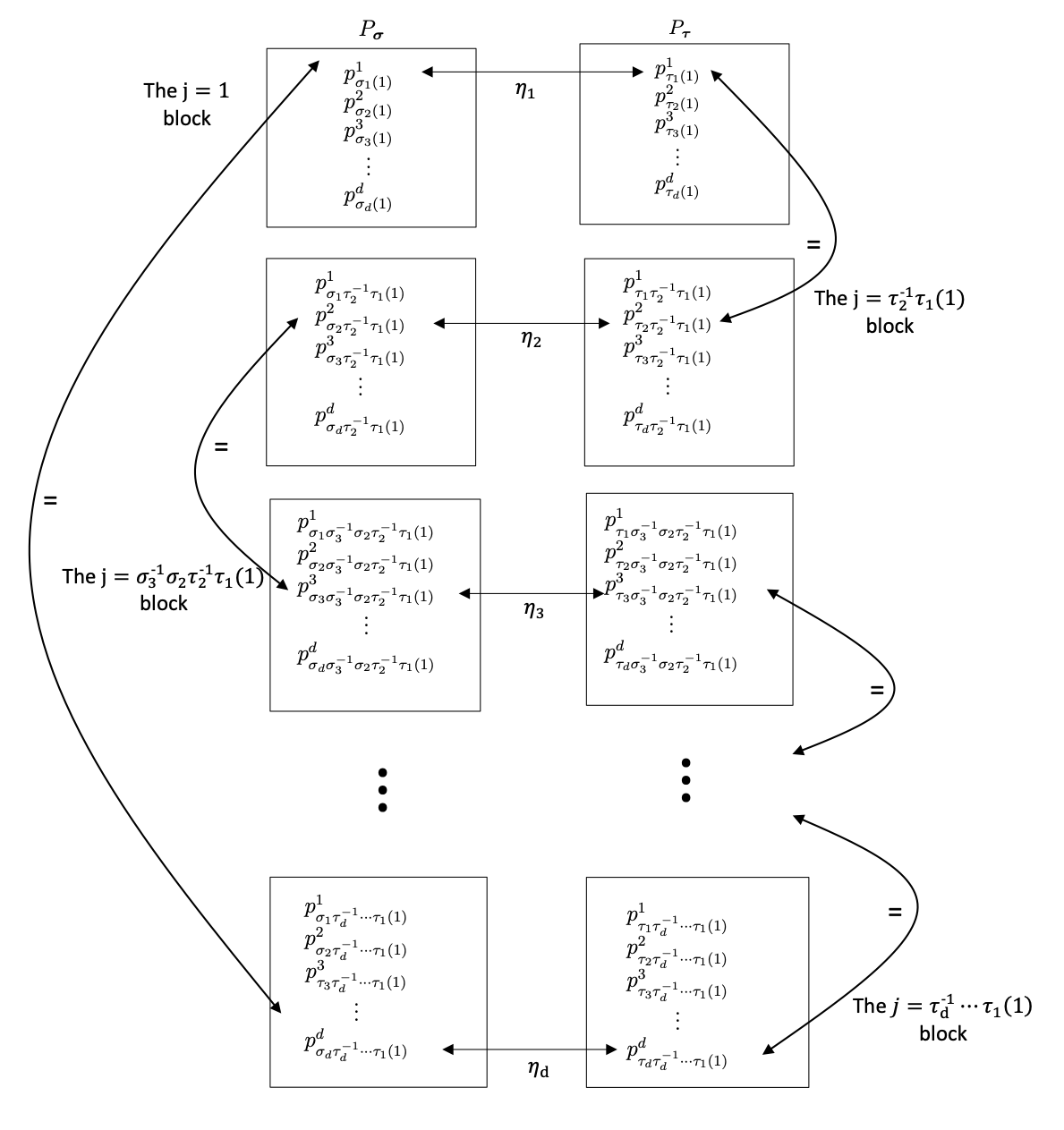
Figure 1. If we wish to avoid rapid decay we must connect up all points in a path. If $(\boldsymbol{\sigma},\boldsymbol{\tau})$ obeys (20) then the path is a loop

There are two important facts that come out of the weaving process which we will record here

1. The condition (20) depends on the transitions $\sigma_{1}^{-1}\sigma_{d}$, $\tau_{d}^{-1}\tau_{d-1}$, etc rather than on individual $\sigma_{m}$ and $\tau_{m}$. So we should average over all $P_{\boldsymbol{\sigma}}$, $P_{\boldsymbol{\tau}}$ which have the same transitions.

2. For every $j=1,\dots,N$ we produce a loop, each loop involved $d$ points. We could start the loop at any other $m$ (rather than $m=1$) the loop condition remains the same. We could also start from $\tau_{1}(j)$ rather than $\sigma_{1}(j)$. Doing so switches the roles of $\boldsymbol{\sigma}$ and $\boldsymbol{\tau}$ in the loop condition (and so is associated with taking the Hermitian conjugate of the related matrix).

We will first treat the case where $d$ is even. The we will see how to embed the odd dimensional project into a problem in dimension $d+1$.

2.1. The even dimensional case

We construct matrix $\mathcal{M}$ with whose trace is given by a sum of loops. By obtaining a lower bound on the trace (using the eigenvector $\mathcal{X}_{\mathds{1}_{\mathbb{P}}}$ of $\mathcal{W}$) we can then obtain control on the size of $N$.

First we will define matrices that average over elements with the same transitions. Here and henceforth we will use mod $d$ clock arithmetic when describing the $\sigma_{m}$ so that $\sigma_{d}=\sigma_{0}$.

Definition 2.2.

For $(\boldsymbol{\sigma},\boldsymbol{\tau})\in(S_{N})^{d}\times(S_{N})^{d}$ we say that

$$\boldsymbol{\sigma}\sim_{ev}\boldsymbol{\tau}$$

if for all even $m\leq d$

(22) $$\sigma_{m}^{-1}\sigma_{m-1}=\tau^{-1}_{m}\tau_{m-1}.$$

We say that

$$\boldsymbol{\sigma}\sim_{odd}\boldsymbol{\tau}$$

if for all odd $m\leq d$

(23) $$\sigma_{m}^{-1}\sigma_{m-1}=\tau_{m}^{-1}\tau_{m-1}.$$

Note that $\sim_{ev}$ and $\sim_{odd}$ are equivalence relations. Let $|[\boldsymbol{\sigma}]_{ev}|$ be the size of the equivalence class of $\boldsymbol{\sigma}$ under $\sim_{ev}$. If $\boldsymbol{\tau}\sim_{ev}\boldsymbol{\sigma}$ then the $\tau_{m}$ for $m$ even can be chosen independently with the $\tau_{m}$, $m$ odd determined by (22). Therefore, $|[\boldsymbol{\sigma}]_{ev}|=(S_{N})^{d/2}=D^{1/2}$. A similar argument shows that the $\sim_{odd}$ equivalence classes have the same size.

We now define matrices associated with the equivalence relations.

(24) $$\mathcal{A}_{ev}(\boldsymbol{\sigma},\boldsymbol{\tau})=\frac{1}{D^{1/2}}\begin{cases}1&\boldsymbol{\sigma}\sim_{ev}\boldsymbol{\tau}\\ 0&\text{otherwise,}\end{cases}$$

(25) $$\mathcal{A}_{odd}(\boldsymbol{\sigma},\boldsymbol{\tau})=\frac{1}{D^{1/2}}\begin{cases}1&\boldsymbol{\sigma}\sim_{odd}\boldsymbol{\tau}\\ 0&\text{otherwise.}\end{cases}$$

Clearly both $\mathcal{A}_{ev}$ and $\mathcal{A}_{odd}$ are an Hermitian projections. Note that $\mathcal{X}_{\mathds{1}_{\mathbb{P}}}$ is an eigenvector (with eigenvalue $1$) of both $\mathcal{A}_{ev}$ and $\mathcal{A}_{odd}.$

We will study the matrix

(26) $$\mathcal{M}=\left(\mathcal{A}_{ev}\mathcal{A}_{odd}+\mathcal{A}_{odd}\mathcal{A}_{ev}\right)\mathcal{W}$$

and will see that its trace consists of a sum over loops. Both $\mathcal{W}$ and $\left(\mathcal{A}_{ev}\mathcal{A}_{odd}+\mathcal{A}_{odd}\mathcal{A}_{ev}\right)$ are clearly Hermitian. The matrix $\mathcal{W}$ is positive semi-definite (as it is $TT^{\star}$ of another operator) and, as we will now show, so is $\left(\mathcal{A}_{ev}\mathcal{A}_{odd}+\mathcal{A}_{odd}\mathcal{A}_{ev}\right)$. Therefore their product, $\mathcal{M}$ has only positive eigenvalues and we can lower bound the trace by the single eigenvalue that we know.

For convenience notate

(27) $$\mathcal{A}=\left(\mathcal{A}_{ev}\mathcal{A}_{odd}+\mathcal{A}_{odd}\mathcal{A}_{ev}\right).$$

To analyse the eigenvalues of $\mathcal{A}$ we need to introduce an auxiliary operator.

Let

(28) $$\mathcal{C}(\boldsymbol{\sigma},\boldsymbol{\tau})=\begin{cases}1&\sigma_{m+1}=\tau_{m}\text{ for all }1\leq m\leq d\\ 0&\text{otherwise.}\end{cases}$$

Note that $\mathcal{C}$ permutes the entries of a vector and so is unitary. In fact $\mathcal{C}^{d}=\operatorname{Id}$ so the eigenvalues of $\mathcal{C}$ are the $d$-th roots of unity. Associated with the matrix $\mathcal{C}$ we define the map $\mathfrak{c}:(S_{N})^{d}\to(S_{N})^{d}$ by

$$\mathfrak{c}(\sigma_{1},\sigma_{2},\dots,\sigma_{d})=(\sigma_{2},\sigma_{3},\dots,\sigma_{d},\sigma_{1})$$

Note that

$$\mathcal{C}\mathcal{V}_{\boldsymbol{\sigma}}=\mathcal{V}_{\mathfrak{c}^{-1}(\sigma)}$$

Lemma 2.3.

The matrices $\mathcal{A}_{ev}$ and $\mathcal{A}_{odd}$ are similar with similarity transform $\mathcal{C}$. The matrix $\mathcal{C}^{2}$ commutes with both $\mathcal{A}_{ev}$ and $\mathcal{A}_{odd}$.

Proof.

The matrix

$$\mathcal{C}\mathcal{A}_{ev}\mathcal{C}^{-1}(\boldsymbol{\sigma},\boldsymbol{\tau})=\frac{1}{D^{1/2}}\begin{cases}1&\mathfrak{c}(\boldsymbol{\sigma})\sim_{ev}\mathfrak{c}(\boldsymbol{\tau})\\ 0&\text{otherwise}\end{cases}$$

The requirement $\mathfrak{c}(\boldsymbol{\sigma})\sim_{ev}\mathfrak{c}(\boldsymbol{\tau})$ enforces

$$\sigma_{3}^{-1}\sigma_{2} =\tau_{3}^{-1}\tau_{2}$$

$$\sigma_{5}^{-1}\sigma_{4} =\tau_{5}^{-1}\tau_{4}$$

$$\vdots$$

$$\sigma_{d-1}^{-1}\sigma_{d-2} =\tau_{d-1}^{-1}\tau_{d-2}$$

$$\sigma_{1}^{-1}\sigma_{d} =\tau_{1}^{-1}\tau_{d}$$

or $\boldsymbol{\sigma}\sim_{odd}\boldsymbol{\tau}$. So indeed $\mathcal{A}_{odd}=\mathcal{C}\mathcal{A}_{ev}\mathcal{C}^{-1}$. Now

$$\mathcal{C}^{2}\mathcal{A}_{ev}(\boldsymbol{\sigma},\boldsymbol{\tau})=\frac{1}{D^{1/2}}\begin{cases}1&\mathfrak{c}^{2}(\boldsymbol{\sigma})\sim_{ev}\boldsymbol{\tau}\\ 0&\text{otherwise}\end{cases}$$

The requirement $\mathfrak{c}^{2}(\boldsymbol{\sigma})\sim_{ev}\boldsymbol{\tau}$ enforces

$$\sigma_{4}^{-1}\sigma_{3} =\tau_{2}^{-1}\tau_{1}$$

$$\sigma_{6}^{-1}\sigma_{5} =\tau_{4}^{-1}\tau_{3}$$

$$\vdots$$

$$\sigma_{d}^{-1}\sigma_{d-1} =\tau_{d-2}^{-1}\tau_{d-3}$$

$$\sigma_{2}^{-1}\sigma_{1} =\tau_{d}^{-1}\tau_{d-1}$$

which is the same as requiring $\boldsymbol{\sigma}\sim_{ev}\mathfrak{c}^{-2}(\boldsymbol{\tau})$. A similar argument shows that $\mathcal{C}^{2}$ commutes with $\mathcal{A}_{odd}$. The key point driving the commutation identities is that the set of even (or odd) transitions are mapped to even (or odd) transitions by $\mathcal{C}^{2}$. ∎

Lemma 2.4.

The matrix $\mathcal{A}$ given by (27) is positive semi-definite.

Proof.

Clearly it is Hermitian. Since both $\mathcal{A}_{ev}$ and $\mathcal{A}_{odd}$ are projections their eigenvalues are in $\{0,1\}$ we denote $\mathfrak{I}_{ev}$ and $\mathfrak{I}_{odd}$ the subspaces spanned by the eigenvectors of eigenvalue 1 associated with $\mathcal{A}_{ev}$ and $\mathcal{A}_{odd}$ respectively.

Because $\mathcal{A}_{ev}$ and $\mathcal{A}_{odd}$ are projections we can write

$$(\mathcal{A}_{ev}+\mathcal{A}_{odd})^{2}=\mathcal{A}_{ev}+\mathcal{A}_{odd}+\mathcal{A}.$$

So if we were able to show that the non-zero eigenvalues of $\mathcal{A}_{ev}+\mathcal{A}_{odd}$ were all at least $1$ then we could conclude that the non-zero eigenvalues of $\mathcal{A}$ are positive. This is what we shall do.

First, using the similarity relationship,

$$\mathcal{A}_{ev}+\mathcal{A}_{odd}=\mathcal{A}_{ev}+\mathcal{C}\mathcal{A}_{ev}\mathcal{C}^{-1}$$

and so

$$(\mathcal{A}_{ev}+\mathcal{A}_{odd})\mathcal{C}=\mathcal{A}_{ev}\mathcal{C}+\mathcal{C}\mathcal{A}_{ev}.$$

However also using the commutation relationship for $\mathcal{C}^{2}$

$$\mathcal{C}(\mathcal{A}_{ev}+\mathcal{A}_{odd}) =\mathcal{C}\mathcal{A}_{ev}+\mathcal{C}^{2}\mathcal{A}_{ev}\mathcal{C}^{-1}$$

$$=\mathcal{A}_{ev}\mathcal{C}+\mathcal{C}\mathcal{A}_{ev}.$$

Therefore $\mathcal{C}$ commutes with $\mathcal{A}_{ev}+\mathcal{A}_{odd}$. So we can find a complete set of joint eigenvectors for $\mathcal{C}$ and $\mathcal{A}_{ev}+\mathcal{A}_{odd}$. Now assume that $v$ is just such a joint eigenvector with $\lambda\neq 0$ eigenvalue for $\mathcal{A}_{ev}+\mathcal{A}_{odd}$. Its eigenvalue for $\mathcal{C}$ is a $d$-th root of unitary which we write as $e^{i\theta}$. We will assume that $v$ is normalised so $\left|\!\left|{v}\right|\!\right|=1$. Then

$$\lambda v =(\mathcal{A}_{ev}+\mathcal{C}\mathcal{A}_{ev}\mathcal{C}^{-1})v$$

$$=\mathcal{A}_{ev}v+e^{-i\theta}\mathcal{C}\mathcal{A}_{ev}v$$

Now $\mathcal{A}_{ev}v\in\mathfrak{I}_{ev}$ therefore we can write $v$ as

$$v=w_{1}+w_{2}$$

where $w_{1}\in\mathfrak{I}_{ev}$ and $w_{2}=e^{-i\theta}\mathcal{C}w_{1}$. Since $\mathcal{A}_{ev}$ and $\mathcal{A}_{odd}$ are similar with similarity transform $\mathcal{C}$ we have that $w_{2}\in\mathfrak{I}_{odd}$. Since $\mathcal{C}$ is unitary $\left|\!\left|{w_{1}}\right|\!\right|=\left|\!\left|{w_{2}}\right|\!\right|$. Now

$$\lambda =\langle v,(\mathcal{A}_{ev}+\mathcal{A}_{odd})v\rangle$$

$$=\langle v,w_{1}+\mathcal{A}_{odd}w_{1}+\mathcal{A}_{ev}w_{2}+w_{2}\rangle$$

$$=1+\langle w_{1},\mathcal{A}_{odd}w_{1}\rangle+\langle w_{2},\mathcal{A}_{odd}w_{1}\rangle+\langle w_{1},\mathcal{A}_{ev}w_{2}\rangle+\langle w_{2},\mathcal{A}_{ev}w_{2}\rangle$$

$$=1+\left|\!\left|{w_{1}}\right|\!\right|^{2}\left(\langle\hat{w}_{1},\hat{w}_{2}\rangle+\langle\hat{w}_{2},\hat{w}_{1}\rangle+\langle\hat{w}_{1},\mathcal{A}_{odd}\hat{w}_{1}\rangle+\langle\hat{w}_{2},\mathcal{A}_{ev}\hat{w}_{2}\rangle\right).$$

The matrices $\mathcal{A}_{ev}$ and $\mathcal{A}_{odd}$ are orthogonal projections so both $\langle\hat{w}_{1},\mathcal{A}_{odd}\hat{w}_{1}\rangle$ and $\langle\hat{w}_{2},\mathcal{A}_{ev}\hat{w}_{2}\rangle$ are positive real numbers. They are equal to the magnitudes of the orthogonal projection of $\hat{w}_{1}$ onto $\mathfrak{I}_{odd}$ and of $\hat{w}_{2}$ onto $\mathfrak{I}_{ev}$ respectively. On the other hand $|\langle\hat{w}_{1},\hat{w}_{2}\rangle|$ is the magnitude of the projection of $\hat{w}_{1}$ onto $\hat{w}_{2}$ or vice-versa. Therefore since $\hat{w}_{1}\in\mathfrak{I}_{ev}$ and $\hat{w}_{2}\in\mathfrak{I}_{odd}$,

$$|\langle\hat{w}_{1},\hat{w}_{2}\rangle|\leq\langle\hat{w}_{2},\mathcal{A}_{ev}\hat{w}_{2}\rangle\quad\text{and}\quad|\langle\hat{w}_{1},\hat{w}_{2}\rangle|\leq\langle\hat{w}_{1},\mathcal{A}_{odd}\hat{w}_{1}\rangle$$

and so

$$\lambda\geq{}1.$$

∎

So we may conclude that $\mathcal{A}$ is positive semi-definite and therefore that $\mathcal{M}$ has positive eigenvalues. We now use that to state a lower bound on the trace of $\mathcal{M}$.

Proposition 2.5.

Let $\mathcal{M}=\mathcal{A}\mathcal{W}$. Then

$$\text{Trace}(\mathcal{M})\geq{}\left(\lambda^{-\frac{\gamma dN}{2}}2^{-(k-1)N}\right)^{2}.$$

Proof.

We will exploit the fact that $\mathcal{X}_{\mathbb{P}}$ is a joint eigenvector (with eigenvalues $1$ and $\Lambda$ respectively) of $\mathcal{A}_{ev}$, $\mathcal{A}_{odd}$ and $\mathcal{W}$. Therefore it is an eigenvector of $\mathcal{M}$ with eigenvalue $\Lambda$. From (18) we have seen that

$$\Lambda\geq{}\left(\lambda^{-\frac{\gamma dN}{2}}2^{-(k-1)N}\right)^{2}.$$

Since all the eigenvalues of $\mathcal{M}$ are non-negative

$$\text{Trace}(\mathcal{M})\geq{}\alpha\geq{}\left(\lambda^{-\frac{\gamma dN}{2}}2^{-(k-1)N}\right)^{2}.$$

∎

On the other hand we will show, in Proposition 2.7, that the trace of $\mathcal{M}$ involves sums over loops and this will lead to an upper bound on the trace. The two bounds together control the growth of $N$. First we prove that $\mathcal{A}$ does indeed give us the sum over loops. We say that $\boldsymbol{\sigma}$ weaves with $\boldsymbol{\tau}$, notated $\boldsymbol{\sigma}\mathscr{W}\boldsymbol{\tau}$ if

(29) $$\sigma_{1}^{-1}\sigma_{d}\tau_{d}^{-1}\tau_{d-1}\cdots\tau^{-1}_{2}\tau_{1}=e$$

Lemma 2.6.

The matrices $\mathcal{A}_{odd}\mathcal{A}_{ev}$ and $\mathcal{A}_{ev}\mathcal{A}_{odd}$ are given by,

(30) $$\mathcal{A}_{odd}\mathcal{A}_{ev}=\frac{1}{D^{1-\frac{1}{d}}}\begin{cases}1&\boldsymbol{\sigma}\mathscr{W}\boldsymbol{\tau}\\ 0&\text{ otherwise}\end{cases}$$

(31) $$\mathcal{A}_{ev}\mathcal{A}_{odd}=\frac{1}{D^{1-\frac{1}{d}}}\begin{cases}1&\boldsymbol{\tau}\mathscr{W}\boldsymbol{\sigma}\\ 0&\text{ otherwise}\end{cases}$$

Proof.

Since they are Hermitian conjugates of each other it is only necessary to prove (30).

$$\mathcal{A}_{odd}\mathcal{A}_{ev}(\boldsymbol{\sigma},\boldsymbol{\tau})=\frac{1}{D}\sum_{\begin{subarray}{c}\boldsymbol{\mu}\sim_{odd}\boldsymbol{\sigma}\\ \boldsymbol{\mu}\sim_{ev}\boldsymbol{\tau}\end{subarray}}1.$$

Let’s first examine a necessary condition for $\mathcal{A}_{odd}\mathcal{A}_{ev}(\boldsymbol{\sigma},\boldsymbol{\tau})$ to be nonzero. Clearly we require that there be at least one $\boldsymbol{\mu}$ with the same odd transitions as $\boldsymbol{\sigma}$ and the same even transitions as $\boldsymbol{\tau}$. Now

$$(\mu_{1}^{-1}\mu_{d})(\mu_{d}^{-1}\mu_{d-1})\cdots(\mu_{3}^{-1}\mu_{2})(\mu_{2}^{-1}\mu_{1})=e$$

so we must have that

$$(\sigma_{1}^{-1}\sigma_{d})(\tau_{d}^{-1}\tau_{d-1})\cdots(\sigma_{3}^{-1}\sigma_{2})(\tau_{2}^{-1}\tau_{1})=e$$

or $\boldsymbol{\sigma}\mathscr{W}\boldsymbol{\tau}$. If $\boldsymbol{\mu}$ has the same odd transitions as $\boldsymbol{\sigma}$ and the same even transitions as $\boldsymbol{\tau}$ and we know one $\mu_{m}$ (for instance $\mu_{1}$) the other $\mu_{m^{\prime}}$ can be calculated from the transitions. So if $(\boldsymbol{\sigma},\boldsymbol{\tau})$ satisfy the necessary condition $\boldsymbol{\sigma}\mathscr{W}\boldsymbol{\tau}$ there are $|S_{N}|=D^{\frac{1}{d}}$ $\boldsymbol{\mu}$ that can appear in the sum. Therefore we have established (30). ∎

We are now in a position to find an upper bound on the trace of $\mathcal{M}$.

Proposition 2.7.

If $\mathcal{M}=\mathcal{A}\mathcal{W}$ then

(32) $$\text{Trace}(\mathcal{M})\leq CN^{-N(d-1)}\lambda^{-\gamma dN}\lambda^{\epsilon N}.$$

Proof.

We have seen that in order to avoid rapid decay of $\boldsymbol{U}(P_{\boldsymbol{\sigma}},P_{\boldsymbol{\tau}})$ we can must be able to construct sequences

$$p_{\sigma_{1}(j)}^{1}\xleftrightarrow[\eta_{1}]{}p_{\tau_{1}(j)}^{1}\xleftrightarrow[\eta_{2}]{}p_{\sigma_{1}\tau_{2}^{-1}\tau_{1}(j)}^{2}\xleftrightarrow[\eta_{3}]{}p^{3}_{\tau_{3}\sigma_{3}^{-1}\sigma_{2}\tau_{2}^{-1}\tau_{1}(j)}\xleftrightarrow[\eta_{4}]{}\cdots\xleftrightarrow[\eta_{d}]{}p^{d}_{\sigma_{d}\tau_{d}^{-1}\tau_{d-1}\cdots\tau_{2}^{-1}\tau_{1}.}$$

and this closes to be a loop if

(33) $$\sigma_{d}\tau_{d}^{-1}\tau_{d-1}\cdots\tau_{2}^{-1}\tau_{1}=\sigma_{1}\Rightarrow\sigma_{1}^{-1}\sigma_{d}\tau_{d}^{-1}\tau_{d-1}\cdots\tau_{2}^{-1}\tau_{1}=e$$

that is $\boldsymbol{\sigma}\mathscr{W}\boldsymbol{\tau}$. Note that we could have started from $\tau_{1}$ in that case the condition to close the loop becomes

(34) $$\tau_{1}^{-1}\tau_{d}\sigma_{d}^{-1}\sigma_{d-1}\cdots\sigma_{2}^{-1}\sigma_{1}=e$$

that is $\boldsymbol{\tau}\mathscr{W}\boldsymbol{\sigma}$.

Now consider a trace element of $\mathcal{M}$, $\mathcal{M}(P_{\boldsymbol{\sigma}},P_{\boldsymbol{\sigma}})$. This is given by

$$\frac{1}{D^{2-\frac{1}{d}}}\left(\sum_{\boldsymbol{\sigma}\mathscr{W}\boldsymbol{\mu}}\boldsymbol{U}(P_{\boldsymbol{\mu}},P_{\boldsymbol{\sigma}})+\sum_{\boldsymbol{\mu}\mathscr{W}\boldsymbol{\sigma}}\boldsymbol{U}(P_{\boldsymbol{\mu}},P_{\boldsymbol{\sigma}})\right)$$

so these elements do obey a loop condition. For notational convenience we will notate the points that make up the loop as $a_{1},\dots,a_{d}$.

Figure 2. We produce a closed loop involving $a_{1},\dots,a_{d}$ and the directions $\eta_{1},\dots\eta_{d}$.

Assume first that these are distinct points in the sense that for each $a_{i}$

$$a_{i}\notin\mathcal{U}_{\epsilon}^{\star}(a_{i+1}).$$

They must therefore lie in a $(d-1)$-dimension hyperplane, that is

(35) $$\frac{a_{1}-a_{2}}{|a_{1}-a_{2}|}\wedge\frac{a_{2}-a_{3}}{|a_{2}-a_{3}|}\wedge\cdots\wedge\frac{a_{d-1}-a_{d}}{|a_{d-1}-a_{d}|}=0.$$

On the other hand we have assumed that

(36) $$|\eta_{1}\wedge\cdots\wedge\eta_{d}|\neq 0$$

and that for each $i$ $\frac{a_{i}-a_{i+1}}{|a_{i}-a_{i+1}|}\in 2\mathcal{U}(\eta_{m})$ for some $m$. Therefore (35) is in contradiction to (36). So some of the pairs $(a_{i},a_{i+1})$ must be the “same” up to the uncertainty principle $a_{i}\in\mathcal{U}_{\epsilon}^{\star}(a_{i+1})$. However the way we have set up our points there is only one $a_{j}\in\mathcal{U}_{\epsilon}^{\star}(a_{i+1})$ and so $a_{i}=a_{i+1}$ and we can contract the cycle and we can apply the same argument again.

Figure 3. In this case ($d=4$) we have $a_{1}=a_{2}$ so we can collapse the loop on the left to that on the right.

Therefore the only possibility is that all the $a_{i}$ are in $\mathcal{U}_{\epsilon}(a_{1})$, which would require $\boldsymbol{\mu}=\boldsymbol{\sigma}$. In fact if the permutations are not quite equal but differ only at a small number of sites the decay from the product kernels isn’t enough to ignore these terms. To use obtain enough decay we need to assume that $\boldsymbol{\mu}$ and $\boldsymbol{\sigma}$ disagree at a positive proportion of sites.

First we will treat the sum where $\boldsymbol{\mu}\mathscr{W}\boldsymbol{\sigma}$ (the other sum follows by the same argument).

For some $\delta>0$ (but assumed to be small) let

(37) $$\mathfrak{D}^{\delta}(\boldsymbol{\sigma})=\left\{\boldsymbol{\mu}\,\Bigg{|}\begin{subarray}{c}\boldsymbol{\mu}\mathscr{W}\boldsymbol{\sigma}\\ d_{H}(\boldsymbol{\mu},\boldsymbol{\sigma})\leq\delta N\end{subarray}\right\}$$

where $d_{H}(\cdot,\cdot)$ is the Hamming distance. Now suppose that $\boldsymbol{\mu}\in(\mathfrak{D}^{\delta}(\boldsymbol{\sigma}))^{c}$. There are $M\geq{}\delta N$ pairs $(m,j)$ so that $\mu_{m}(j)\neq\sigma_{m}(j)$, we may as well assume that $M$ is divisible by $d$. Let $(m,j)$ be a such a pair. We start a weaving process from this point to construct a non-trivial loop

$$p_{\mu_{m}(j)}\xleftrightarrow[\eta_{m}]{}p_{\sigma_{m}(j)}\xleftrightarrow[\eta_{m+1}]{}p_{\mu_{m+1}\sigma_{m+1}^{-1}\sigma_{m}(j)}\xleftrightarrow[\eta_{m+3}]{}\cdots\xleftrightarrow[\eta_{m-1}]{}p_{\mu_{m}(j)}.$$

Therefore one of the kernels

$$\underleftrightarrow{\eta_{m}}(p_{\mu_{m}(j)},p_{\sigma_{m}(j)})$$

$$\underleftrightarrow{\eta_{m+1}}(p_{\mu_{m+1}\sigma_{m+1}^{-1}\sigma_{m}(j)},p_{\sigma_{m}(j)})$$

$$\vdots$$

$$\underleftrightarrow{\eta_{m-1}}(p_{\mu_{m}(j)},p_{\sigma_{m-1}^{-1}\cdots\sigma_{m}(j)})$$

must rapidly decay as $C_{Q}\lambda^{-Q}$ for any natural number $Q$. Possibly we have used some other $(m^{\prime},j^{\prime})$ such that $\mu_{m^{\prime}}(j^{\prime})\neq\sigma_{m^{\prime}}(j^{\prime})$ in this loop but at most we have only used $d$ of them, so we have $M-d$ remaining. Pick one of those and repeat the process to general another rapidly decaying kernel. We then have $M-2d$ remaining. Repeat this process $M/d$ times to produce $M/d$ kernels each rapidly decaying. Therefore

$$|\boldsymbol{U}(P_{\boldsymbol{\mu}},P_{\boldsymbol{\sigma}})| \leq C_{Q}\lambda^{-\gamma\left(dN-\frac{M}{d}\right)}(\lambda^{-Q})^{\frac{M}{d}}$$

$$\leq C_{Q}\lambda^{-\gamma\left(dN-\frac{M}{d}\right)}\lambda^{-Q\delta N}.$$

So by making $Q$ large enough (dependent only on $\delta$) we obtain

(38) $$|\boldsymbol{U}(P_{\boldsymbol{\mu}},P_{\boldsymbol{\sigma}})|\lesssim\lambda^{-AN}$$

for $A$ as large as we like. So these terms make a negligible contribution to the trace.

Now it remains to treat the terms where $\boldsymbol{\mu}\in\mathfrak{D}^{\delta}(\boldsymbol{\sigma})$. For these terms we accept a trivial bound of $\lambda^{-\gamma dN}$ (from the kernel bound, assumption (7)). However there are relatively few such terms. Given a particular set of (no more than $\delta N$) sites $(m,j)$ where $\mu_{m}(j)\neq\sigma_{m}(j)$ there can be no more than $N^{\delta N}$ ways to chose $\boldsymbol{\mu}$. There are no more than $2^{dN}$ ways to pick the sets of sites so

(39) $$|\mathfrak{D}(\boldsymbol{\sigma})|\leq 2^{dN}N^{\delta N}.$$

Combining (38) and (39) we obtain the estimate

$$|\mathcal{M}(\boldsymbol{\sigma},\boldsymbol{\sigma})|\leq D^{-2+\frac{1}{d}}2^{Nd}\lambda^{-\gamma dN}\left(N^{\delta N}+\lambda^{-AN}\right).$$

Recalling that $D=|S_{N}|^{d}=(N!)^{d}$ and $N\leq C\lambda^{d}$ we then have that for a suitable choice of $\delta$ (dependent on $\epsilon$);

$$\text{Trace}(\mathcal{M})\leq CN^{-N(d-1)}\lambda^{-\gamma dN}\lambda^{\epsilon N}.$$

∎

We can now finally prove Theorem 1.4. Putting together the lower and upper bounds for $\text{Trace}(\mathcal{M})$ (Propositions 2.5 and 2.7 respectively) we have

$$\lambda^{-\gamma dN}2^{-2(k-1)N}\leq CN^{-N(d-1)}\lambda^{-\gamma dN}\lambda^{\epsilon N}$$

so

$$N\leq C2^{\frac{2(k-1)}{d-1}}\lambda^{\frac{\epsilon}{d-1}}.$$

Theorem 1.4 then follows from the observation that

$$N\geq{}\frac{|\Omega_{k}|}{|\mathcal{U}_{\epsilon}^{\star}|},$$

2.2. The odd dimensional case

We now turn our attention to the case where $d$ is odd. Fortunately we can treat this case by embedding it in dimension $d+1$.

Define the matrix

$$\widetilde{\mathcal{W}}=\mathcal{W}\otimes\operatorname{Id}$$

where $\otimes$ is the Kronecker product and $\operatorname{Id}$ is the $(S_{N})\times(S_{N})$ identity matrix. In the coordinate system given by $\mathcal{V}_{\boldsymbol{\sigma}}$ and $\boldsymbol{\sigma}=(\boldsymbol{\sigma}^{\prime},\sigma_{d+1})$.

$$\widetilde{\mathcal{W}}=\frac{1}{D}U(P_{\boldsymbol{\sigma}^{\prime}},P_{\boldsymbol{\tau}^{\prime}})\operatorname{Id}(\sigma_{d+1},\tau_{d+1}).$$

Note that $\mathcal{X}_{\mathds{1}_{\mathbb{P}}}$ is still an eigenvector of $\widetilde{\mathcal{W}}$ with eigenvalue $\alpha$ and $\widetilde{\mathcal{W}}$ is still a positive semi-definite matrix. As in the even case we form the matrix

$$\mathcal{M}=\mathcal{A}\widetilde{\mathcal{W}}$$

this is still a matrix with positive eigenvalues so the lower bound for the trace remains the same.

The form of the trace elements remains the same. That is they are given by

$$\frac{1}{D^{2-\frac{1}{d}}|S_{N}|}\left(\sum_{\boldsymbol{\mu}\mathscr{W}\boldsymbol{\sigma}}\boldsymbol{U}(P_{\boldsymbol{\mu}^{\prime}},P_{\boldsymbol{\sigma}^{\prime}})\operatorname{Id}(\mu_{d+1},\sigma_{d+1})+\sum_{\boldsymbol{\sigma}\mathscr{W}\boldsymbol{\mu}}\boldsymbol{U}(P_{\boldsymbol{\mu}^{\prime}},P_{\boldsymbol{\sigma}^{\prime}})\operatorname{Id}(\mu_{d+1},\sigma_{d+1})\right).$$

The extra factor of $|S_{N}|^{-1}$ comes from the definition of the matrices $\mathcal{A}_{ev}$ and $\mathcal{A}_{odd}$. If $\boldsymbol{\mu}\mathscr{W}\boldsymbol{\sigma}$

$$\mu_{1}^{-1}\mu_{d+1}\sigma_{d+1}^{-1}\sigma_{d}\mu_{d}^{-1}\mu_{d-1}\cdots\sigma_{2}^{-1}\sigma_{1})=e$$

but since $\mu_{d+1}=\sigma_{d+1}$ (otherwise $\operatorname{Id}(\mu_{d+1},\sigma_{d+1})=0$) this reduces to

$$\mu_{1}^{-1}\sigma_{d}\mu_{d}^{-1}\mu_{d-1}\cdots\sigma_{2}^{-1}\sigma_{1}=e$$

which gives a closed loop for the weaving process in odd dimensions. A similar argument gives a closed loop for the $\boldsymbol{\sigma}\mathscr{W}\boldsymbol{\mu}$ terms.

Therefore we can still obtain the bound

$$|\mathcal{M}(P_{\boldsymbol{\sigma}},P_{\boldsymbol{\sigma}})|\leq D^{-2+\frac{1}{d}}|S_{N}|^{-1}\lambda^{-\gamma dN}\left(N^{(1+d\delta)N}+\lambda^{-AN}\right)$$

and since this is a $D|S_{N}|\times D|S_{N}|$ matrix the upper bound for the trace remains the same. That is

$$\text{Trace}(\mathcal{M})\leq CN^{-N(d-1)}A^{2dN}\lambda^{-\gamma dN}\lambda^{\epsilon N}$$

and so by the same reasoning as the case where $d$ is even we obtain

$$|\Omega_{k}|\leq C2^{\frac{2(k-1)}{d-1}}\lambda^{\epsilon}|\mathcal{U}_{\epsilon}^{\star}|.$$

Remark 2.8.

The proof of Theorem 1.4 makes the critical numerology of $p=\frac{2}{d-1}$ (morally equivalent to the linear numerology of $p=\frac{2d}{d-1}$) quite clear. Suppose we are estimating $T$ over a region $\Omega$ covered by $N$ uncertainty sets $\mathcal{U}_{\epsilon}(p_{j})$ so that $Tu(p_{j})$ are all around the same size. In our $TT^{\star}$ argument we average over all possible loops with $d$ points chosen in a set of $N$ objects and find that the major contribution comes from the trivial loops that only consist of one point. Therefore since the number of loops of $d$ points grows as $N^{d}$ and the number of trivial loops grows as $N$ we expect a $N^{-(d-1)}$ improvement over the trivial $TT^{\star}$ estimate, corresponding to a $N^{-\frac{d-1}{2}}$ improvement over the trivial estimate for $T$. So if the saturating $L^{\infty}$ estimate is $\lambda^{-\frac{\gamma}{2}}$ then

$$\left|\!\left|{Tu}\right|\!\right|_{L^{p}(\Omega)}\lesssim\lambda^{-\frac{\gamma}{2}}N^{-\frac{d-1}{2}}|\mathcal{U}^{\star}|^{\frac{1}{p}}N^{\frac{1}{p}}$$

For $p>\frac{2}{d-1}$ the decay from the simultaneous saturation result is enough to counteract the growth in measure. But for $p<\frac{2}{d-1}$ the reverse is true. In general if we are able to construct loops of $M$ objects where only the trivial loop makes a significant contribution we can obtain a $N^{-(M-1)}$ improvement for the $TT^{\star}$ estimate which will correspond to a critical $p=\frac{2}{M-1}$.

Remark 2.9.

The abstract set up of constructing loops on the diagonal of an energy matrix is completely independent of the context from which the energy matrix was obtained. We can understand the energy matrix $\mathcal{W}$ as

$$\mathcal{W}=\mathcal{W}_{1}\otimes\mathcal{W}_{2}\otimes\cdots\otimes\mathcal{W}_{d}$$

where each of the $\mathcal{W}_{m}$ is the energy matrix associated with the $m$-th operator, crucially each measures the interactions on the same set of points (but with different operators). Therefore these techniques could be applied in any setting that has the following features;

1. A set of points $\{p_{1},\dots,p_{N}\}$.

2. An energy matrix $\mathcal{W}=\mathcal{W}_{1}\otimes\mathcal{W}_{2}\otimes\cdots\otimes\mathcal{W}_{d}$ where each of the $\mathcal{W}_{m}$ is a positive definite energy matrix with dimension $N!$.

3. The elements of $\mathcal{W}_{m}(\sigma,\tau)$ decay rapidly unless

   $$p_{\sigma(j)}\xleftrightarrow{\text{$m$-th condition}}{}p_{\tau(j)}\quad\text{for all }j.$$

   The $m$-th condition can be anything, in this example it was a requirement around direction.

4. Any loops of points $p_{j_{1}},\dots,p_{j_{d}}$ connected by the $d$ conditions is impossible unless the loop is trivial.

One could also look at constructing other illegal ensembles (other than loops) on the diagonal. These would require construction of a positive definite Hermitian matrix that effects the required structure.

3. Multilinear models for the Bochner-Riesz problem

We will look at multilinear models for the Bochner-Riesz problem. The parameter dependent problem which asks about the $L^{p}(B_{1}(0))\to L^{p}(B_{1}(0))$ mapping norms of the operator

$$Tf=\lambda^{\frac{d-1}{2}}\int e^{i\lambda|x-y|}a(x,y)f(y)dy$$

where $a(x,y)$ is supported in $\frac{\epsilon}{2}\leq|x-y|\leq\epsilon$. With a partition of unity we may as well also assume that $a(x,y)$ is supported in region

$$\left|\frac{x-y}{|x-y|}-(1,0,\cdots,0)\right|\leq\epsilon.$$

The Bochner-Riesz conjecture asserts that

$$\left|\!\left|{T}\right|\!\right|_{L^{p}(B_{1}(0))\to L^{p}(B_{1}(0))}\lesssim\lambda^{\frac{d-1}{2}-\frac{d}{p}+\epsilon}\text{ for all }p>p_{c}=\frac{2d}{d-1}.$$

The $L^{\infty}$ estimate is trivial and so by interpolation it is sufficient to prove an estimate of the form

$$\left|\!\left|{T}\right|\!\right|_{L^{p_{c}}(B_{1}(0))}\lesssim_{\epsilon}\lambda^{\epsilon}\left|\!\left|{f}\right|\!\right|_{L^{p_{c}}(B_{1}(0))}.$$

Here we will study multilinear models arising from $T$. These are $d$ products of operators $T_{m}$ where

$$T_{m}f=\lambda^{\frac{d-1}{2}}\int e^{i\lambda|x-y|}a_{m}(x,y)f(y)dy$$

with $a_{m}$ supported in a region

$$\left|\frac{x-y}{|x-y|}-\eta_{m}\right|\leq\text{ small }.$$

Exactly what “small” is will depend on the model. Note that we can already use Theorem 1.4 to treat some cases. If we assume that for a set of $\{\eta_{1},\dots,\eta_{d}\}$ $|\eta_{m}-e_{1}|\leq\lambda^{-\beta}$ we have $a_{m}(x,y)$ supported where

$$\left|\frac{x-y}{|x-y|}-\eta_{m}\right|\leq\lambda^{-\beta}$$

and for any collection of $r\leq d$ distinct $\eta_{m_{r}}$,

$$|\eta_{m_{1}}\wedge\cdots\wedge\eta_{m_{r}}|\geq{}C\lambda^{-\beta|r|}$$

we can define the following uncertainty system.

1. The set of directions is given by $\{\eta_{m}\}$

2. The uncertainty set $\mathcal{U}(\eta_{m})$ is given by

   $$\left\{\xi\in S^{d-1}\Big{|}|\xi-\eta_{m}|\leq\lambda^{-\beta}\text{ or }|\xi+\eta_{m}|\leq\lambda^{-\beta}\right\}$$

3. the one parameter family of set $\mathcal{U}_{\epsilon}^{\star}(x)$ are given by

   $$\left\{y\in\mathbb{R}^{d}\Bigg{|}\begin{subarray}{c}|x(1)-y(1)|\leq\lambda^{-1+2\beta+\epsilon},\\ |x(l)-y(l)|\leq\lambda^{-1+\beta+\epsilon},l=2,\dots,d\end{subarray}\right\}$$

The size and shape of $\mathcal{U}_{\epsilon}^{\star}(x)$ is determined by the uncertainty principle and the curvature of $S^{d-1}$ an arises from standard stationary phase calculations.

Note that the way the wedge products degenerate as $\lambda\to\infty$ is symmetric. In this section we will treat the non-symmetric case. For example in dimension three one may have

$$|\eta_{1}\wedge\eta_{2}|\geq{}1$$

but

$$\lambda^{-\beta}\leq|\eta_{1}\wedge\eta_{2}\wedge\eta_{3}|\leq 2\lambda^{-\beta}.$$

To treat these sort of cases we develop an uncertainty system associated with each scale, this system involves nesting various uncertainty set and then defining different length loops at different levels.

These cases are all “enemies” of the Bochner-Riesz conjecture in the sense that Theorem 3.3 were not true the counterexamples for that would give rise to Bochner-Riesz counterexamples. Therefore Theorem 3.3 greatly restricts the ways in which the Bochner-Riesz conjecture could fail.

Throughout this construction and proof we will fix $\epsilon>0$ on which all estimates will depend. We will track the form of that dependence. Let $A=\{\alpha_{i}\}$ be a collection of scales $\alpha_{i}=\lambda^{-\epsilon(1+i)}$ with $i=0,\dots,I$ such that $I$ is the first integer so that $\lambda^{-\epsilon(i+I)}\leq\lambda^{-\frac{1}{2}+\frac{\epsilon}{2}}$. We say that $\alpha_{I}$ is the degenerate scale and all other scales are non-degenerate. We will describe a multilinear model of scale $\boldsymbol{\alpha}$ and orientation $e_{1}$. Let $\boldsymbol{\alpha}=(\alpha_{i_{2}},\alpha_{i_{3}},\dots,\alpha_{i_{d}})$ with each $\alpha_{i_{l}}\in A$ and with the $\alpha_{i_{l}}$ listed in decreasing size.

Definition 3.1.

A multilinear model consists of a set of scales $\boldsymbol{\alpha}=(\alpha_{i_{2}},\dots,\alpha_{i_{d}})$, a set of vectors $\{\eta_{m}\}_{m=1}^{d}\subset\mathbb{S}^{d-1}$ and an operator obeying the following conditions:

Scales

The $\alpha_{i_{l}}=\lambda^{-(\epsilon+i_{l})}$ are listed in decreasing size.

Directions

If $\boldsymbol{\alpha}$ does not contain the degenerate scale $\alpha_{I}$ then the set of $\boldsymbol{\eta}=\{\eta_{m}\}_{m=1}^{d}\subset\mathbb{S}^{d-1}$ obeys the non-degeneracy and control conditions

$$c_{1}\alpha_{i_{2}}\leq|\eta_{1}\wedge\eta_{2}|\leq C_{1}\alpha_{i_{2}}$$

$$c_{2}\alpha_{i_{2}}\alpha_{i_{3}}\leq|\eta_{1}\wedge\eta_{2}\wedge\eta_{3}|\leq C_{2}\alpha_{i_{2}}\alpha_{i_{3}}$$

$$\vdots$$

$$c_{d}\alpha_{i_{2}}\cdots\alpha_{i_{w}}\leq|\eta_{1}\wedge\cdots\wedge\eta_{d}|\leq C_{d}\alpha_{i_{2}}\cdots\alpha_{i_{w}}$$

If the degenerate scale $\alpha_{I}$ does appear in $\boldsymbol{\alpha}$, $r_{I}$ times we omit the last $r_{l}$ non-degeneracy conditions and only have the control conditions.

Operator

The operator $T_{\boldsymbol{\alpha},\boldsymbol{\eta}}:(L^{2}(B_{1}(0)))^{d}\to C^{\infty}(B_{1}(0))$ is defined by

$$T_{\boldsymbol{\alpha},\boldsymbol{\eta}}(f_{1}\otimes\cdots\otimes f_{d})=\mathcal{R}\circ\bigotimes_{m=1}^{d}T_{\boldsymbol{\alpha},\eta_{m}}f_{m}$$

where $\mathcal{R}:(C^{\infty}(B_{1}(0)))^{d}\to C^{\infty}(B_{1}(0))$ is the restriction to the diagonal $x^{m}=x^{m^{\prime}}$ and

$$T_{\boldsymbol{\alpha},\eta_{m}}f=\int K_{\boldsymbol{\alpha},\eta_{m}}(x,y)f(y)dy$$

$$K_{\boldsymbol{\alpha},\eta_{m}}(x,y)=e^{i\lambda|x-y|}a_{m}(x,y)$$

(40) $$a_{m}(x,y)=\prod_{l=2}^{d}\chi_{\epsilon}\left(\alpha_{i_{l}}^{-1}\left|\frac{x(l)-y(l)}{|x-y|}-\eta_{m}(l)\right|\right)$$

where the coordinate system has been chosen so that the $(e_{1},\dots,e_{d-1})$ plane corresponds with the $(\eta_{1},\dots,\eta_{d-1})$ plane in the non-degenerate case. In the case that there is a degenerate scale appearing $r_{I}$ times the $(e_{1},\dots,e_{d-r_{I}})$ plane corresponds with the $(\eta_{1},\dots,e_{d-r_{I}})$ plane.

The main theorem of this section, Theorem 3.3 asserts that

(41) $$\left|\!\left|{T_{\boldsymbol{\alpha},\boldsymbol{\eta}}(f_{1}\otimes\cdots\otimes f_{m})}\right|\!\right|_{L^{p_{c}/d}}\lesssim\lambda^{\epsilon}\prod_{l=2}^{d}\alpha_{i_{l}}^{-\frac{1}{2}}\prod_{m=1}^{d}\left|\!\left|{f_{m}}\right|\!\right|_{L^{2}}.$$

We will use a simultaneous saturation argument that nests scales and allows us to use different loop length at different levels of the nesting. We need to prepare the ground a bit first. Critical to the simultaneous saturation result is the decay properties of entries in the energy matrix. Just as in Theorem 1.4 we will construct this matrix via a $TT^{\star}$ argument. The decay of entries in the matrix will therefore be determined by the critical point analysis (in $y$) of the phase function

$$\phi(x,y,z)=|x-y|-|y-z|.$$

The critical points of this phase function are well understood. By fixing $x$ at zero and integrating $y$ in spheres of fixed radius it is easy to see that the critical point appear at the intersections between the sphere and the line joining $x$ and $z$. The critical points are non-degenerate and the Hessian has determinant bounded below by $|x-z|^{d-1}$. If we can apply the stationary phase formula it is then straightforward to determine whether or not a particular matrix element rapidly decays. However, the introduction of the scales $\alpha_{i_{l}}$ may disrupt such an argument as the usual stationary phase set up requires that the symbol be smooth and independent of the parameter $\lambda$. In our case we have smooth symbols, but their regularity bounds are $\lambda$ dependent. Since we are not interested in developing a full asymptotic formula for these integrals we do not need the full strength of the stationary phase formula and can instead use Van der Corput’s Lemma which just gives the size of the oscillating integral. The proof of Van der Corput’s Lemma progresses by isolating the critical point with a cut of function of scale $(\lambda H)^{-1/2}$ where $H$ is the size of the determinant of the Hessian. Therefore this argument still holds so long as any loss in regularity in the symbol is no worse than $(\lambda H)^{1/2}$ per derivative.

The smallest scale appearing in the multilinear operator is $\alpha_{i_{d}}$. Therefore if we want to perform a critical point analysis in all the $y$ variables we require that

$$(\lambda|x-z|)^{1/2}\geq{}\lambda^{\frac{\epsilon}{2}}\alpha_{i_{d}}^{-1}\Rightarrow|x-z|\geq{}\lambda^{-1+\epsilon}\alpha_{i_{d}}^{-2}.$$

We could freeze the $y(d)$ variable and perform stationary phase in the other variables, the next smallest scale is $\alpha_{i_{d-1}}$ and to be able to progress that critical point calculation we require that

$$(\lambda|x-z|)^{1/2}\geq{}\lambda^{\frac{\epsilon}{2}}\alpha_{i_{d-1}}^{-1}\Rightarrow|x-z|\geq{}\lambda^{-1+\epsilon}\alpha_{i_{d-1}}^{-2}$$

and so on. These length scales allow us to define uncertainty sets. Since we have localised around $e_{1}$ we will see that we can effectively replace $|x-z|$ with $|x(1)-z(1)|$. We will form tubes with long directions (the $e_{1}$ direction) on the scales $\lambda^{-1+\epsilon}\alpha_{i_{d}}^{-2},\dots,\lambda^{-1+\epsilon}\alpha_{i_{2}}^{-2}$ with the smaller scales nested inside the larger ones. The restriction on the variables $l=2,\dots,d$ are determined by the angular cut off and the length scale. At the first step consider a set of tubes with centres $q_{j_{d}}$

$$\mathscr{T}_{q_{(j_{d})}}=\left\{x\in\mathbb{R}^{d}\Bigg{|}\begin{subarray}{c}|x(1)-q_{(j_{d})}(1)|\leq\epsilon^{4}\lambda^{-1+\epsilon}\alpha_{i_{d}}^{-1}\\ |x(l)-q_{(j_{d})}(l)|\leq 2\lambda^{-1+\epsilon}\alpha_{i_{d}}^{-2}\alpha_{i_{l}}\text{ for }l=2,\dots,d\end{subarray}\right\}$$

chosen so that the tubes tile $B_{1}(0)$. Therefore

$$\left|\!\left|{T_{\boldsymbol{\alpha},\boldsymbol{\eta}}}\right|\!\right|_{L^{\frac{2}{d-1}}(B_{1}(0))}\leq\left(\sum_{q_{(j_{d})}}\left|\!\left|{T_{\boldsymbol{\alpha},\boldsymbol{\eta}}}\right|\!\right|_{L^{\frac{2}{d-1}}(\mathscr{T}_{q_{(j_{d})}})}^{\frac{2}{d-1}}\right)^{\frac{d-1}{2}}$$

Applying the multilinear Hölder inequality on each tube separately we then have

$$\left|\!\left|{\prod_{m=1}^{d}T_{\boldsymbol{\alpha},\eta_{m}}f_{m}(\cdot)}\right|\!\right|_{L^{\frac{2}{d-1}}(B_{1}(0))}\leq\left(\sum_{q_{(j_{d})}}\left|\!\left|{\prod_{m=1}^{d-1}T_{\boldsymbol{\alpha},\eta_{m}}f_{m}(\cdot)}\right|\!\right|^{\frac{2}{d-1}}_{L^{\frac{2}{d-2}}(\mathscr{T}_{(q_{j_{d}})})}\left|\!\left|{T_{\boldsymbol{\alpha},\eta_{d}}f_{d}}\right|\!\right|^{\frac{2}{d-1}}_{L^{2}(\mathscr{T}_{q_{(j_{d})}})}\right)^{\frac{d-1}{2}}$$

Now we tile each $\mathscr{T}_{q_{(j_{d})}}$ with tubes $\mathscr{T}_{q_{(j_{d},j_{d-1})}}$ with centres $q_{(j_{d},j_{d-1})}$

$$\mathscr{T}_{q_{(j_{d},j_{d-1})}}=\left\{x\in\mathscr{T}_{q_{(j_{d})}}\Bigg{|}\begin{subarray}{c}|x(1)-q_{(j_{d},j_{d-1})}(1)|\leq\epsilon^{4}\lambda^{-1+\epsilon}\alpha_{i_{d-1}}^{-1}\\ |x(l)-q_{(j_{d},j_{d-1})}(l)|\leq 2\lambda^{-1+\epsilon}\alpha_{i_{d-1}}^{-2}\alpha_{i_{l}}\text{ for }l=2,\dots,d-1\\ |x(d)-q_{(j_{d},j_{d-1})}(d)|\leq\lambda^{-1+\epsilon}\alpha_{i_{d}}^{-1}\end{subarray}\right\}$$

and so have

$$\left|\!\left|{\prod_{m=1}^{d}T_{\boldsymbol{\alpha},\eta_{m}}f_{m}(\cdot)}\right|\!\right|_{L^{\frac{2}{d-1}}(B_{1}(0))}\\ \leq\left(\sum_{q_{(j_{d})}}\left(\sum_{q_{(j_{d},j_{d-1})}}\left|\!\left|{\prod_{m=1}^{d-1}T_{\boldsymbol{\alpha},\eta_{m}}f_{m}(\cdot)}\right|\!\right|_{L^{\frac{2}{d-2}}(\mathscr{T}_{q_{(j_{d},j_{d-1})}})}^{\frac{2}{d-2}}\left|\!\left|{T_{\boldsymbol{\alpha},\eta_{d}}f_{d}}\right|\!\right|_{L^{2}(\mathscr{T}_{q_{(j_{d})}})}^{\frac{2}{d-2}}\right)^{\frac{d-2}{d-1}}\right)^{\frac{d-1}{2}}$$

Again we apply Hölder on each $\mathscr{T}_{q_{(j_{d},j_{d-1})}}$ and then tile with tubes $\mathscr{T}_{q_{(j_{d},j_{d-1},j_{d-2})}}$ given by

$$\mathscr{T}_{q_{(j_{d},j_{d-1},j_{d-2})}}=\left\{x\in\mathscr{T}_{q_{(j_{d},j_{d-1})}}\Bigg{|}\begin{subarray}{c}|x(1)-q_{(j_{d},j_{d-1},j_{d-2})}(1)|\leq\epsilon^{4}\lambda^{-1+\epsilon}\alpha_{i_{d-2}}^{-1}\\ |x(l)-q_{(j_{d},j_{d-1},j_{d-2})}(l)|\leq 2\lambda^{-1+\epsilon}\alpha_{i_{d-2}}^{-2}\alpha_{i_{l}}\text{ for }l=2,\dots,d-2\\ |x(l)-q_{(j_{d},j_{d-1},j_{d-2})}(l)|\leq\lambda^{-1+\epsilon}\alpha_{i_{l}}^{-1}\text{ for }l=d-1,d\end{subarray}\right\}$$

and continue in this fashion to get that

(42) $$\left|\!\left|{\prod_{m=1}^{d}T_{\boldsymbol{\alpha},\eta_{m}}f_{m}}\right|\!\right|_{L^{\frac{2}{d-1}}}\\ \leq\left(\sum_{q_{(j_{d})}}\left(\sum_{q_{(j_{d},j_{d-1})}}\cdots\left(\sum_{q_{(j_{d},\dots,j_{2})}}\left|\!\left|{\prod_{m=1}^{2}T_{\boldsymbol{\alpha},\eta_{m}}f_{m}}\right|\!\right|^{2}_{L^{2}(\mathscr{T}_{q_{(j_{d},\dots,j_{2})}})}\right.\right.\right.\\ \left.\left.\left.\times\prod_{m=3}^{d}\left|\!\left|{T_{\boldsymbol{\alpha},\eta_{m}}f_{m}}\right|\!\right|^{2}_{L^{2}(\mathscr{T}_{q_{(j_{d},\dots,j_{m})}})}\right)^{\frac{1}{2}}\cdots\right)^{\frac{d-2}{d-1}}\right)^{\frac{d-1}{2}}.$$

We will control (42) by performing a similtaneous saturation argument, the objects that we insert into the argument are

$$\prod_{m=1}^{2}T_{\boldsymbol{\alpha},\eta_{m}}f_{m}(p_{(j_{d},\dots,j_{2})})\prod_{m=3}^{d}\left|\!\left|{T_{\boldsymbol{\alpha},\eta_{m}}f_{m}}\right|\!\right|_{L^{2}(\mathscr{T}_{q_{(j_{d},\dots,j_{m})}})}$$

where $p_{(j_{d},\dots,j_{2})}$ is a point in $\mathscr{T}_{q_{(}j_{d},\dots,j_{2})}$. For notational convenience we set

$$\boldsymbol{G}(p_{(j_{d},\dots,j_{2})})=\prod_{m=1}^{2}T_{\boldsymbol{\alpha},\eta_{m}}f_{m}(p_{(j_{d},\dots,j_{2})})\prod_{m=3}^{d}\left|\!\left|{T_{\boldsymbol{\alpha},\eta_{m}}f_{m}}\right|\!\right|_{L^{2}(\mathscr{T}_{q_{(j_{d},\dots,j_{m})}})}$$

We now define some uncertainty systems, that are set to match the tubes $\mathscr{T}_{q_{(j_{d},\dots,j_{2})}}$.

We index our uncertainty systems by $n$ which runs from $n=2$ to $n=d$ (the index $n$ gives the effective dimension). We fix an coordinate system so that $(e_{1},\dots,e_{w})$ lines up with $(\eta_{1},\dots,\eta_{w})$. We define an uncertainty system $\mathfrak{U}_{n}(\epsilon,\lambda)$.

1. The set of directions is given by $\{\eta_{m}\}$.

2. The uncertainty sets $\mathcal{U}_{n}(\eta_{m})$ are given by

   $$\mathcal{U}_{n}(\eta_{m})=\left\{\xi\in S^{n-1}\Big{|}\begin{subarray}{c}|\xi(l)-\eta_{m}(l)|\leq\alpha_{i_{l}}\quad l=2,\dots,d\\ \text{or }|\xi(l)+\eta_{m}(l)|\leq\alpha_{i_{l}}\quad l=2,\dots,d\end{subarray}\right\}$$

3. The one parameter family of sets $\mathcal{U}_{n,\epsilon}^{\star}(x)$ are defined by

   $$\mathcal{U}_{n,\epsilon}^{\star}(x)=\left\{y\in\mathbb{R}^{n}\Bigg{|}\begin{subarray}{c}|y(1)-x(1)|\leq\epsilon^{4}\lambda^{-1+\epsilon}\alpha_{i_{n}}^{-2}\text{ and }\\ |y(l)-x(l)|\leq 2\lambda^{-1+\epsilon}\alpha_{i_{n}}^{-2}\alpha_{i_{l}},\text{ for }l=2,\dots,n\\ |y(l)-x(l)|\leq 2\lambda^{-1+\epsilon}\alpha_{i_{l}}^{-1}\text{ for }l=n+1,\dots,d\end{subarray}\right\}$$

Now we are ready to locate some points to feed to the simultaneous saturation argument.

Theorem 3.2.

We can find a sequence of tubes $\mathscr{T}^{(j_{d})},\mathscr{T}^{(j_{d},j_{d-1})},\dots,\mathscr{T}^{(j_{d},\dots,j_{2})}$ and a point $p_{(j_{d},\dots,j_{2})}\in\mathscr{T}^{(j_{d},\dots,j_{2})}$ such that:

1. There are

   $$\begin{array}[]{lll}N_{d}&\text{level $d$ tubes }\mathscr{T}^{(j_{d})}&\text{each containing}\\ \vskip 1.42271pt\\ N_{d-1}&\text{level $d-1$ tubes }\mathscr{T}^{(j_{d},j_{d-1})}&\text{each containing}\\ \vskip 1.42271pt\\ \vdots&\vdots&\vdots\\ \vskip 1.42271pt\\ N_{2}&\text{level $2$ tubes }\mathscr{T}^{(j_{d},j_{d-1},\dots,j_{2})}&\end{array}$$

2. For any $p_{(j_{d},\dots,j_{2})}$ and $p_{(j^{\prime}_{d},\dots,j^{\prime}_{2})}$,

   $$\frac{1}{2}\boldsymbol{G}(p_{(j^{\prime}_{d},\dots,j^{\prime}_{2})})\leq\boldsymbol{G}(p_{(j_{d},\dots,j_{2})})\leq 2\boldsymbol{G}(p_{(j^{\prime}_{d},\dots,j^{\prime}_{2})})$$

3. If $x\in\mathscr{T}^{(j_{d},\dots,j_{n})}$ and $y\in\mathscr{T}^{(j^{\prime}_{d},\dots,j^{\prime}_{n})}$ for $(j_{d},\dots,j_{n})\neq(j^{\prime}_{d},\dots,j^{\prime}_{2})$ then

   $$x\notin\mathcal{U}_{n,\epsilon}^{\star}(y)$$

4. $$\left|\!\left|{\prod_{m=1}^{d}T_{\boldsymbol{\alpha},\eta_{m}}f_{m}}\right|\!\right|_{L^{\frac{2}{d-1}}}\leq\lambda^{\epsilon}|\mathscr{T}^{(1,\dots,1)}|^{\frac{1}{2}}G(p_{(1,\dots,1)})\prod_{n=2}^{d}N_{n}^{\frac{n-1}{2}}$$

Proof.

We write

$$X=\left(\sum_{q_{(j_{d})}}X_{q_{(j_{d})}}\right)^{\frac{d-1}{2}}$$

where

$$X_{q_{(j_{d})}}=\left(\sum_{q_{(j_{d},j_{d-1})}}\cdots\left(\sum_{q_{(j_{d},\dots,j_{2})}}\left|\!\left|{\prod_{m=1}^{2}T_{\boldsymbol{\alpha},\eta_{m}}f_{m}}\right|\!\right|^{2}_{L^{2}(\mathscr{T}_{q_{(j_{d},\dots,j_{2})}})}\right.\right.\\ \left.\left.\times\prod_{m=3}^{d}\left|\!\left|{T_{\boldsymbol{\alpha},\eta_{m}}f_{m}}\right|\!\right|^{2}_{L^{2}(\mathscr{T}_{q_{(j_{d},\dots,j_{m})}})}\right)^{\frac{1}{2}}\cdots\right)^{\frac{d-2}{d-1}}$$

For $V$ so that $2^{V}\geq{}\lambda^{d+1}$ define

$$Z_{d,v} =\left\{j_{d}\Bigg{|}2^{-v-1}\sum_{k_{d}}X_{q_{(k_{d})}}<X_{q_{(j_{d})}}\leq 2^{-v}\sum_{k_{d}}X_{q_{(k_{d})}}\right\}\quad 0\leq v<V$$

$$Z_{d,V} =\left\{j_{d}\Bigg{|}X_{q_{(j_{d})}}\leq 2^{-V}\sum_{k_{d}}X_{q_{(k_{d})}}\right\}$$

Since there are only logarithmically (in $\lambda$) man $v$s there must be some $v_{1}$ so that

$$\sum_{j_{d}\in Z_{d,v_{1}}}X_{q_{(j_{d})}}\geq{}\frac{\sum_{k_{d}}X_{(q_{k_{d}})}}{d\log(\lambda)}.$$

Note that $v_{1}$ cannot be $V$. For a loss of a constant depending only on dimension we may also assume that the tubes are well spaced so that if $x$ and $y$ are on different tubes

$$|x(1)-y(1)|\geq{}10\lambda^{-1+\epsilon}\alpha_{i_{n}}^{-2}$$

and

$$|x(l)-y(l)|\geq{}10\lambda^{-1+\epsilon}\alpha_{i_{n}}^{-2}\alpha_{i_{l}}.$$

Let $N_{d}(1)$ be the number of terms in the sum. As each of these terms is, up to a factor of $2$, the same size we can say that for each $j_{d}\in Z_{d,j_{1}}$,

$$X_{q_{(j_{d})}}\geq{}\frac{\delta\sum_{k_{d}}X_{(q_{k_{d}})}}{N_{d}(1)\log(\lambda)}=\frac{\delta X^{\frac{2}{d-1}}}{N_{d}(1)\log(\lambda)}$$

where $\delta$ may be a small constant but is independent of $\lambda$. Now for each such $j_{d}$ re-name the $\mathscr{T}_{q_{j_{d}}}$ as $\mathscr{T}^{(j_{d})}$ and write each $X_{q_{(j_{d})}}$ as

$$X_{q_{(j_{d})}}=\left(\sum_{q_{(j_{d},j_{d-1})}}X_{q_{(j_{d},j_{d-1})}}\right)^{\frac{d-2}{d-1}}$$

where

$$X_{q_{(j_{d},j_{d-1})}}=\left(\sum_{q_{(j_{d},j_{d-1},j_{d-2})}}\cdots\left(\sum_{q_{(j_{d},\dots,j_{2})}}\left|\!\left|{\prod_{m=1}^{2}T_{\boldsymbol{\alpha},\eta_{m}}f_{m}}\right|\!\right|^{2}_{L^{2}(\mathscr{T}_{q_{(j_{d},\dots,j_{2})}})}\right.\right.\\ \left.\left.\times\prod_{m=3}^{d}\left|\!\left|{T_{\boldsymbol{\alpha},\eta_{m}}f_{m}}\right|\!\right|^{2}_{L^{2}(\mathscr{T}_{q_{(j_{d},\dots,j_{m})}})}\right)^{\frac{1}{2}}\cdots\right)^{\frac{d-3}{d-2}}$$

and define

$$Z_{d-1,v}^{(j_{d})} =\left\{j_{d-1}\Bigg{|}2^{-(v+1)}\sum_{k_{d-1}}X_{q_{(j_{d},k_{d-1})}}<X_{q_{(j_{d},j_{d-1})}}\leq 2^{-v}\sum_{k_{d-1}}X_{q_{(j_{d},k_{d-1})}}\right\}\quad 0\leq v<V$$

$$Z_{d-1,V}^{(j_{d})} =\left\{j_{d-1}\Bigg{|}X_{q_{(j_{d},j_{d-1})}}\leq 2^{-V}\sum_{k_{d-1}}X_{q_{(j_{d},k_{d-1})}}\right\}.$$

By the arguments of our first step we can produce a $v_{2}^{(j_{d})}$ so that

$$\sum_{j_{d-1}\in Z^{(j_{d})}_{d-1,v_{2}^{(j_{d})}}}X_{q_{(j_{d},j_{d-1})}}\geq{}\frac{\sum_{k_{d-1}}X_{q_{(j_{d},k_{d-1})}}}{d\log(\lambda)}.$$

Further for each $j_{d}$ there are only $d\log(\lambda)$ options for $v^{(j_{d})}_{2}$ so there must be some $v_{2}$ so that there are at least $\frac{N_{d}(1)}{d\log(\lambda)}$ values of $j_{d}$ with $v_{2}^{(j_{d})}=v_{2}$. We discard all other values of $j_{d}$ then we have $N_{d}(2)\geq\frac{N_{d}(1)}{d\log(\lambda)}$ tubes $\mathscr{T}^{(j_{d})}$ so that

$$X_{q_{(j_{d})}}\geq{}\frac{\delta X^{\frac{2}{d-1}}}{N_{d}(1)\log(\lambda)}\geq{}\frac{\delta X^{\frac{2}{d-1}}}{N_{d}(2)(d\log(\lambda))^{2}}$$

and on each of these tubes

$$\sum_{j_{d-1}\in Z^{(j_{d})}_{2,v_{2}}}X_{q_{(j_{d},j_{d-1})}}\geq{}\frac{\sum_{k_{d-1}}X_{q_{(j_{d},k_{d})}}}{d\log(\lambda)}.$$

Let $N^{(j_{d})}_{d-1}(1)$ be the number of terms in left hand sum. By the way we have chosen $v_{2}$, the $N^{(j_{d})}_{d-1}(1)$ can only differ by a factor of $2$. Let $N_{d-1}(1)=\min_{j_{d}}\{N^{(j_{d})}_{d-1}(1)\}$ and for any $j_{d}$ such that $N^{(j_{d})}_{d-1}(1)>N_{d-1}(1)$ we discard $N^{(j_{d})}_{d-1}(1)-N_{d-1}(1)$ tubes (the choice of which to discard is arbitrary). The remaining tubes we denote $\mathscr{T}^{(j_{d},j_{d-1})}$ for each $(j_{d},j_{d-1})$

$$X_{q_{(j_{d},j_{d-1})}}\geq{}\frac{\delta\sum_{k_{d-1}}X_{q_{(j_{d},k_{d})}}}{N_{d-1}(1)d\log(\lambda)}=\frac{\delta X^{\frac{d-1}{d-2}}_{q_{(j_{d})}}}{N_{d-1}(1)d\log(\lambda)}.$$

Using the lower bounds for $X_{q_{(}j_{d})}$ we then have

$$X_{q_{(j_{d},j_{d-1})}}\geq{}\frac{\delta^{2}X^{\frac{2}{d-2}}}{N_{d}(2)^{\frac{d-1}{d-2}}N_{d-1}(1)(d\log(\lambda))^{3}}$$

We repeat the process $d-1$ times to obtain

$$\begin{array}[]{lll}N_{d}=N_{d}(d-1)&\text{tubes }\mathscr{T}^{(j_{d})}&\text{each containing}\\ \vskip 1.42271pt\\ N_{d-1}=N_{d-1}(d-2)&\text{tubes }\mathscr{T}^{(j_{d},j_{d-1})}&\text{each containing}\\ \vskip 1.42271pt\\ \vdots&\vdots&\vdots\\ \vskip 1.42271pt\\ N_{2}=N_{2}(1)&\text{tubes }\mathscr{T}^{(j_{d},j_{d-1},\dots,j_{2})}&\end{array}$$

such that

$$X_{(j_{d},\dots,j_{2})}\geq{}\frac{\delta^{d}X^{2}}{N_{d}^{d-1}N_{d-1}^{d-2}\cdots N_{2}(d\log(\lambda))^{d^{2}}}$$

From which we have that

$$X\leq\lambda^{\epsilon}X_{(j_{d},\dots,j_{2})}^{\frac{1}{2}}\prod_{n=2}^{d}N_{n}^{\frac{n-1}{2}}$$

Finally we pick a point $p_{(j_{d},\dots,j_{2})}$ in each of the

$$\mathscr{T}^{(j_{d},\dots,j_{2})}$$

to maximise $\boldsymbol{G}(p_{(j_{d},\dots,j_{2})})$. We may assume that all the $\boldsymbol{G}(p_{(j_{d},\dots,j_{2})})$ are (up to a factor of $2$) the same size by potentially throwing away another $\log(\lambda)$ terms. Since we may always estimate

$$X_{(j_{d},\dots,j_{2})}\leq\boldsymbol{G}(p_{(j_{d},\dots,j_{2})})|\mathscr{T}^{(j_{d},\dots,j_{2})}|^{\frac{1}{2}}$$

we have

$$X\leq\lambda^{\epsilon}\boldsymbol{G}(p_{(1,\dots,1)})|\mathscr{T}^{(1,\dots,1)}|^{\frac{1}{2}}\prod_{n=2}^{d}N_{n}^{\frac{n-1}{2}}.$$

∎

We have $N=\prod_{n=2}^{d}N_{n}$ points $p_{(j_{d},\dots,j_{2})}$ to feed to the simultaneous saturation argument. We say that $(j_{d},\dots,j_{2})$ is the address of the point $p_{(j_{d},\dots,j_{2})}$. Our argument is similar to that of Theorem 1.4 however we allow different averaging at different levels of the address.

Theorem 3.3.

Suppose that $T_{\boldsymbol{\alpha},\boldsymbol{\eta}}$ is an operator associated with a multilinear model, then

(43) $$\left|\!\left|{T_{\boldsymbol{\alpha},\boldsymbol{\eta}}(f_{1}\otimes\cdots\otimes f_{d})}\right|\!\right|_{L^{p_{c}/d}}\lesssim\lambda^{d^{2}\epsilon}\left(\prod_{l=2}^{d}\alpha_{i_{l}}\right)^{-\frac{1}{2}}\prod_{m=1}^{d}\left|\!\left|{f_{m}}\right|\!\right|_{L^{2}}$$

Proof.

First we place an ordering on the $\{p_{(j_{d},\dots,j_{2})}\}$, for instance via an odometer ordering. Abusing notation we will write $j=(j_{d},\dots,j_{2})$ for $j\in\{1,\dots,N\}$ where we mean that $(j_{d},\dots,j_{2})$ is the $j$th address in our ordering. When referring to permutations we understand $(\sigma(j))_{l}$ to be the $j_{l}$ element of the tuple associated with $\sigma(j)$. Again we set

$$P_{\boldsymbol{e}^{\prime}}=(p_{1}^{1},\dots,p_{1}^{d},p_{2}^{1},\dots,p_{N}^{d})$$

where the superscript acts as a tagging and $p_{j}^{m}=p_{j}^{m^{\prime}}$. We write

$$Z=(z_{1}^{1},z_{1}^{2},\dots,z_{N}^{d})$$

and set

$$\boldsymbol{F}(Z)=\prod_{j=1}^{N}\prod_{m=1}^{d}f_{m}(z_{j}^{m}).$$

We set

$$\boldsymbol{T}F(X)=\int\boldsymbol{K}(X,Z)F(Z)dZ$$

where

$$K(X,Z)=\prod_{j=1}^{N}\prod_{m=1}^{d}K_{m}(x_{j}^{m},z_{j}^{m})$$

where $K_{m}(x_{j}^{m},z_{j}^{m})$ is given by, for $m=1,2$

$$K_{m}(x,z)=\lambda^{\frac{d-1}{2}}e^{i\lambda|x-z|}a_{m}(x,z)$$

and for $m=3,\dots,d$

$$K_{m}(x,z)=\lambda^{\frac{d-1}{2}}\int\phi_{x}(v)e^{i\lambda|v-z|}a_{m}(v,z)dv$$

where $\phi_{x}$ is supported in the level $m$ tube that contains $x$ and has $\left|\!\left|{\phi_{x}}\right|\!\right|_{L^{2}}=1$. There is obviously some degree of choice of $\phi_{x}$, we will select one to maximise $L^{2}$ norms on the level $m$ tube. We will need to be able to deal with odd dimensions so we adopt the notation of Theorem 1.4 in the odd dimensional case. Let $\boldsymbol{\sigma}=(\boldsymbol{\sigma}^{\prime},\sigma_{d+1})$, where $\boldsymbol{\sigma}^{\prime}=(\sigma_{1},\dots,\sigma_{d})\in(S_{N})^{d}$ and $D=|S_{N}|^{d}$. Then if

$$P_{\boldsymbol{\sigma}^{\prime}}=(p_{\sigma_{1}(1)}^{1},p_{\sigma_{2}(1)}^{2},\dots,p_{\sigma_{d}(1)}^{d},p_{\sigma_{1}(2)}^{1},\dots,p_{\sigma_{d}(N)}^{d})$$

with an appropriate choice of $\phi_{x_{j}^{m}}$s we have that

$$\boldsymbol{T}\boldsymbol{F}\Big{|}_{P_{\boldsymbol{\sigma}^{\prime}}}\geq\boldsymbol{G}(p_{(1,\dots,1)})^{N}.$$

Let $\mathbb{P}=\{P_{\boldsymbol{\sigma}^{\prime}}\}_{\boldsymbol{\sigma}^{\prime}\in(S_{N})^{d}}$ and let $\boldsymbol{\delta}_{\mathbb{P}}$ be the measure given by

$$\boldsymbol{\delta}_{\mathbb{P}}=\frac{1}{D}\sum_{\boldsymbol{\sigma}^{\prime}\in(S_{N})^{d}}\boldsymbol{\delta}_{P_{\boldsymbol{\sigma}^{\prime}}}$$

where $\boldsymbol{\delta}_{P_{\boldsymbol{\sigma}^{\prime}}}$ is the point measure associated at $P_{\boldsymbol{\sigma}^{\prime}}$. Following the notation of Theorem 1.4 we let

$$\boldsymbol{U}(X,Y)=\prod_{m=1}^{d}\prod_{j=1}^{N}\underleftrightarrow{\eta_{m}}(x_{j}^{m},y_{j}^{m})$$

where $\underleftrightarrow{\eta_{m}}(x,y)$ is given by

(44) $$\underleftrightarrow{\eta_{m}}(x,y)=\int K_{m}(x,z)\overline{K_{m}(z,y)}dz$$

Since the structure of $\boldsymbol{U}(X,Y)$ is the same as as in Theorem 1.4, Lemma 2.1 holds in this case and $\mathds{1}_{\mathbb{P}}$ is an eigenfunction of $\boldsymbol{T}\boldsymbol{T}^{\star}$ with eigenvalue

$$\Lambda\geq\boldsymbol{G}(p_{(1,\dots,1)})^{2N}.$$

We now convert all that information into the energy matrix. Again we order our vectors/matrices by the permutations and talk about the $\boldsymbol{\sigma}$ element of a vector or the $(\boldsymbol{\sigma}^{\prime},\boldsymbol{\tau}^{\prime})$ element of a matrix. If

$$\mathcal{V}_{\boldsymbol{\sigma}^{\prime}}(\boldsymbol{\tau}^{\prime})=\begin{cases}1&\boldsymbol{\tau}^{\prime}=\boldsymbol{\sigma}^{\prime}\\ 0&\boldsymbol{\tau}^{\prime}\neq\boldsymbol{\sigma}^{\prime}\end{cases}$$

then we can use $\{\mathcal{V}_{\boldsymbol{\sigma}^{\prime}}\mid\boldsymbol{\sigma}^{\prime}\in(S_{N})^{d}\}$ as a basis and we denote by $\mathcal{W}$ the matrix associated with $\boldsymbol{T}\boldsymbol{T}^{\star}$ in this basis. So

$$\mathcal{W}(\boldsymbol{\sigma}^{\prime},\boldsymbol{\tau}^{\prime})=\frac{1}{D}\boldsymbol{U}(P_{\boldsymbol{\sigma}^{\prime}},P_{\boldsymbol{\tau}^{\prime}}).$$

Because we will need, on occasion, to work with odd dimensions we will instead work with

$$\widetilde{\mathcal{W}}=\mathcal{W}\otimes\operatorname{Id}_{S_{N}}$$

where $\otimes$ is the Kronecker product and $\operatorname{Id}_{S_{N}}$ is the $(S_{N})\times(S_{N})$ identity matrix. So

$$\widetilde{\mathcal{W}}(\boldsymbol{\sigma},\boldsymbol{\tau})=\frac{1}{D}\boldsymbol{U}(P_{\boldsymbol{\sigma}^{\prime}},P_{\boldsymbol{\tau}^{\prime}})\operatorname{Id}_{S_{N}}(\sigma_{d+1},\tau_{d+1})$$

We now define our averaging operators. They are much the same as those in Theorem 1.4 however this time we will define $d-1$ such operators each acting at a different level of the nesting (so that they commute). At level $n$ the averaging operator

$$\mathcal{A}_{n}=\mathcal{A}_{ev,n}\mathcal{A}_{odd,n}+\mathcal{A}_{odd,n}\mathcal{A}_{ev,n}$$

will produce $n$-loops on the diagonal.

Let’s now do that. Suppose first that $n$ is even. Then define

$$\boldsymbol{\sigma}\sim_{ev,n}\boldsymbol{\tau}$$

if

1. For $m>n$, $\sigma_{m}=\tau_{m}$.

2. For $m\leq n$ and $n^{\prime}\neq n$

   $$(\sigma_{m}(j))_{n^{\prime}}=(\tau_{m}(j))_{n^{\prime}}\quad j=1,\dots,N$$

3. For all even $m\leq n$

   $$(\sigma^{-1}_{m}\sigma_{m-1}(j))_{n}=(\tau_{m}^{-1}\tau_{m-1}(j))_{n}\quad j=1,\dots,N$$

and that

$$\boldsymbol{\sigma}\sim_{odd,n}\boldsymbol{\tau}$$

if

1. For $m>n$, $\sigma_{m}=\tau_{m}$.

2. For $m\leq n$ and $n^{\prime}\neq n$

   $$(\sigma_{m}(j))_{n^{\prime}}=(\tau_{m}(j))_{n^{\prime}}\quad j=1,\dots,N$$

3. For all odd $3\leq m\leq n$

   $$(\sigma^{-1}_{m}\sigma_{m-1}(j))_{n}=(\tau_{m}^{-1}\tau_{m-1}(j))_{n}\quad j=1,\dots,N$$

4. For $m=1$

   $$(\sigma^{-1}_{1}\sigma_{n}(j))_{n}=(\tau_{1}^{-1}\tau_{n}(j))_{n}\quad j=1,\dots,N$$

If $d_{n}$ is odd

$$\boldsymbol{\sigma}\sim_{ev,n}\boldsymbol{\tau}$$

if

1. For $n<m\leq d$, $\sigma_{m}=\tau_{m}$.

2. For $m\leq n,m=d+1$ and $n^{\prime}\neq n$

   $$(\sigma_{m}(j))_{n^{\prime}}=(\tau_{m}(j))_{n^{\prime}}\quad j=1,\dots,N$$

3. For all even $m\leq n$

   $$(\sigma^{-1}_{m}\sigma_{m-1}(j))_{n}=(\tau_{m}^{-1}\tau_{m-1}(j))_{n}\quad j=1,\dots,N$$

4. For $m=d+1$

   $$(\sigma^{-1}_{d+1}\sigma_{n}(j))_{n}=(\tau_{d+1}^{-1}\tau_{n}(j))_{n}\quad j=1,\dots,N$$

and that

$$\boldsymbol{\sigma}\sim_{odd,n}\boldsymbol{\tau}$$

if

1. For $n<m\leq d$, $\sigma_{m}=\tau_{m}$.

2. For $m\leq n,m=d+1$ and $n^{\prime}\neq n$

   $$(\sigma_{m}(j))_{n^{\prime}}=(\tau_{m}(j))_{n^{\prime}}\quad j=1,\dots,N$$

3. For all odd $3\leq m\leq d_{n}$

   $$(\sigma^{-1}_{m}\sigma_{m-1}(j))_{n}=(\tau_{m}^{-1}\tau_{m-1}(j))_{n}\quad j=1,\dots,N$$

4. For $m=1$,

   $$(\sigma^{-1}_{1}\sigma_{d+1}(j))_{n}=(\tau_{1}^{-1}\tau_{d+1}(j))_{n}\quad j=1,\dots,N$$

Essentially these relations freeze everything except the $n$th level of the nesting and then require that at the $n$th level on the nesting $\boldsymbol{\sigma}$ and $\boldsymbol{\tau}$ have the same even/odd transitions. In Lemma 3.6 we confirm that these are equivalence relations and compute the size of the equivalence classes.

$$\Upsilon(n)=\begin{cases}[\boldsymbol{\sigma}]_{\sim_{ev,n}}=[\boldsymbol{\sigma}]_{\sim_{odd,n}}=(N_{n}!)^{\frac{nN}{2N_{n}}}&d_{n}\text{ even }\\ [\boldsymbol{\sigma}]_{\sim_{ev,n}}=[\boldsymbol{\sigma}]_{\sim_{odd,n}}=(N_{n}!)^{\frac{(n+1)N}{2N_{n}}}&d_{n}\text{ odd}\end{cases}$$

Now we define the averaging matrices

(45) $$\mathcal{A}_{ev,n}(\boldsymbol{\sigma},\boldsymbol{\tau})=\frac{1}{\Upsilon(n)}\begin{cases}1&\boldsymbol{\sigma}\sim_{ev,n}\boldsymbol{\tau}\\ 0&\text{ otherwise}\end{cases}$$

(46) $$\mathcal{A}_{odd,n}(\boldsymbol{\sigma},\boldsymbol{\tau})=\frac{1}{\Upsilon(n)}\begin{cases}1&\boldsymbol{\sigma}\sim_{odd,n}\boldsymbol{\tau}\\ 0&\text{ otherwise}\end{cases}$$

Just as before $\mathcal{A}_{ev,n}$ and $\mathcal{A}_{odd,n}$ are Hermitian projections and that the vector of ones is and eigenvector (with eigenvalue $1$). We set

(47) $$\mathcal{A}_{n}=\mathcal{A}_{ev,n}\mathcal{A}_{odd,n}+\mathcal{A}_{odd,n}\mathcal{A}_{ev,n}$$

Since $\mathcal{A}_{n}$ and $\mathcal{A}_{n^{\prime}}$ act at different levels of the nesting they commute (Lemma 3.7). So it is only necessary to establish that each $A_{n}$ is positive semi-definite. This is just an adjustment of the proof the $\mathcal{A}$, Lemma 2.4 is positive semidefinite and so we outsource it to Lemma 3.8.

Finally we set

(48) $$\mathcal{A}=\prod_{n=2}^{d}\mathcal{A}_{n}$$

and

(49) $$\mathcal{M}=\mathcal{A}\widetilde{\mathcal{W}}$$

and it is this matrix for which we will compute the trace. The eigenvalues of $\mathcal{M}$ must be non-negative and we can compute some of them.

For any $p_{(j_{d},\dots,j_{2})}$ we define its reduced address by, if $d$ is even $\tilde{j}=(j_{d},j_{d-2},\dots,j_{2})$ and if $d$ is odd $\tilde{j}=(j_{d-1},j_{d-3},\dots,j_{2})$. That is the reduced address selects the even levels. We write $\widetilde{\sigma(j)}$ for the reduced address of $\sigma(j)$ and say $\sigma\sim_{red}\tau$ if

$$\widetilde{\sigma(j)}=\widetilde{\tau(j)}\text{ for all }j=1,\dots,N.$$

Let $\{\pi\}$ be a set of representatives of the classes under $\sim_{red}$ then define

$$\mathcal{X}_{\pi}(\boldsymbol{\sigma})=\begin{cases}1&\widetilde{\sigma_{d+1}(j)}=\widetilde{\pi(j)}\text{ for all }j=1,\dots,N\\ 0&\text{ otherwise}\end{cases}$$

and claim that $\mathcal{X}_{\pi}$ is an eigenvector with eigenvalue $2^{d-1}\Lambda$ of $\mathcal{M}$. Recall that

$$\widetilde{\mathcal{W}}=\mathcal{W}\otimes\operatorname{Id}_{|S_{N}|}.$$

Now

$$\mathcal{X}_{\pi}=\mathds{1}_{D}\otimes\mathcal{X}_{d+1,\pi}$$

where $\mathds{1}_{D}$ is the $D$ dimensional vector of ones and $\mathcal{X}_{d+1,\pi}$ is the $|S_{N}|$ dimensional vector

$$\mathcal{X}_{d+1,\pi}(\sigma_{d+1})=\begin{cases}1&\widetilde{\sigma_{d+1}(j)}=\widetilde{\pi(j)}\text{ for all }j=1,\dots,N\\ 0&\text{otherwise.}\end{cases}$$

We know that the vector of ones is an eigenvector for $\mathcal{W}$ with eigenvalue $\Lambda$. Therefore $\mathcal{X}_{\pi}$ is an eigenvector of $\widetilde{\mathcal{W}}$ with eigenvalue $\Lambda$. Similarly if $n$ is even

$$\mathcal{A}_{ev,n}=\mathcal{A}_{d,ev,n}\otimes\operatorname{Id}_{|S_{N}|}$$

$$\mathcal{A}_{odd,n}=\mathcal{A}_{d,odd,n}\otimes\operatorname{Id}_{|S_{N}|}$$

where $\mathcal{A}_{d,ev,n}$ and $\mathcal{A}_{d,ev,n}$ are the $D\times D$ matrices defined by dropping the condition on $m=d+1$ in the $\sim_{ev,n}$ and $\sim_{odd,n}$ relations. So $\mathcal{X}_{\pi}$ is an eigenvector, of eigenvalue $1$, of $\mathcal{A}_{ev,n}$. However for $n$ odd the non-trivial part of the action of $\mathcal{A}_{ev,n}$ and $\mathcal{A}_{odd,n}$ takes place at an odd level and $\mathcal{X}_{\pi}$ is symmeterised over the entries at odd levels. So it is also an eigenvector of these matrices, with eigenvalue one. Therefore $\mathcal{X}_{\pi}$ is an eigenvector of eigenvalue $2^{d-1}\Lambda$ of $\mathcal{M}$. There is one such eigenvector/eigenvalue for each $\pi$. Suppose $\sigma\sim_{red}\pi$ and consider those $j$ such that

$$(\sigma(j))_{i}=(\pi(1))_{i}\text{ for all }2\leq i\leq d,i\text{ even}$$

there are

$$\prod_{\begin{subarray}{c}2\leq n\leq d\\ n\text{ odd}\end{subarray}}N_{n}$$

such sites and we may as well assume that they are numbered

$$1\leq j\leq\prod_{\begin{subarray}{c}2\leq n\leq d\\ n\text{ odd}\end{subarray}}N_{n}.$$

There are then

$$\left(\prod_{\begin{subarray}{c}2\leq n\leq d\\ n\text{ odd}\end{subarray}}N_{n}\right)!$$

ways to choose $\sigma(j)$ at these sites. We can use the same argument to count the number of ways to assign $\sigma(j)$ in the next block

$$\left(\prod_{\begin{subarray}{c}2\leq n\leq d\\ n\text{ odd}\end{subarray}}N_{n}\right)+1\leq j\leq 2\prod_{\begin{subarray}{c}2\leq n\leq d\\ n\text{ odd}\end{subarray}}N_{n}.$$

So there are

$$\left[\left(\prod_{\begin{subarray}{c}2\leq n\leq d\\ n\text{ odd}\end{subarray}}N_{n}\right)!\right]^{\frac{N}{\prod_{\begin{subarray}{c}2\leq n\leq d\\ n\text{ odd}\end{subarray}}N_{n}}}$$

elements of the equivalence class. Or alternatively

$$N!\left[\left(\prod_{\begin{subarray}{c}2\leq n\leq d\\ n\text{ odd}\end{subarray}}N_{n}\right)!\right]^{-\frac{N}{\prod_{\begin{subarray}{c}2\leq n\leq d\\ n\text{ odd}\end{subarray}}N_{n}}}$$

distinct equivalence classes. Using Stirling’s approximation for factorial we can say that there are at least

$$C\prod_{\begin{subarray}{c}2\leq n\leq d\\ n\text{ even}\end{subarray}}N_{n}^{N}$$

distinct equivalence classes and since is associated with an eigenvector we can conclude that the trace obeys a lower bound

(50) $$\text{Trace}(\mathcal{M})\geq{}\left(\prod_{\begin{subarray}{c}n=2\\ n\text{ even }\end{subarray}}^{d}N_{n}^{N}\right)\Lambda\geq\left(\prod_{\begin{subarray}{c}2\leq n\leq d\\ n\text{ even }\end{subarray}}^{d}N_{n}^{N}\right)\boldsymbol{G}(p_{(1,\dots,1)})^{2N}.$$

We will now examine the elements of the diagonal of $\mathcal{M}$ and show they are made up of loops which are illegal unless they are trivial (ie all the permutations are the same).

We argue as in the proof of Theorem 1.4 and produce a path

$$p_{\sigma_{1}(j)}^{1}\xleftrightarrow[\eta_{1}]{}p_{\tau_{1}(j)}^{1}\xleftrightarrow[\eta_{2}]{}p_{\sigma_{1}\tau_{2}^{-1}\tau_{1}(j)}^{2}\xleftrightarrow[\eta_{3}]{}p^{3}_{\tau_{3}\sigma_{3}^{-1}\sigma_{2}\tau_{2}^{-1}\tau_{1}(j)}\xleftrightarrow[\eta_{4}]{}\cdots\xleftrightarrow[\eta_{d+1}]{}p_{\sigma_{d}\tau_{d}^{-1}\tau_{d-1}\cdots\tau_{2}^{-1}\tau_{1}}$$

where by the $x\xleftrightarrow[\eta_{m}]{}y$ notation we mean that $x$ and $y$ are related in a way such that the kernel $\underleftrightarrow{\eta_{m}}(x,y)$ does not necessarily rapidly decay. The conditions for avoiding rapid decay, the proof is left to Lemma LABEL:lem:nestdecay, are that for every $1\leq n\leq d$ either

1. $y\in\mathcal{U}_{n,\epsilon}^{\star}(x)$ or;

2. $$\frac{\mathfrak{P}_{d-n}\left(x-y\right)}{\left|\mathfrak{P}_{d-n}(x-y)\right|}\in 2\mathcal{U}_{n}(\eta_{m})$$

   where $\mathfrak{P}_{d-n}$ projects a vector into the plane where the final $d-n$ entries are zero.

In Lemma LABEL:lem:nesttivest we also obtain the trivial bounds for the $\underleftrightarrow{\eta_{m}}(x,y)$. The bounds depend on $m$ but in all cases we at least have that

(51) $$|\underleftrightarrow{\eta_{m}}(x,y)|\leq\lambda^{\frac{d-1}{2}}$$

As before we will refer to this as making a weaving pattern and say that for $n$ even $\boldsymbol{\sigma}$ weaves with $\boldsymbol{\tau}$ at level $n$ (notated $\boldsymbol{\sigma}\mathscr{W}_{n}\boldsymbol{\tau}$) if

$$(\sigma_{1}^{-1}\sigma_{n}\tau_{n}^{-1}\tau_{n-1}\cdots\tau_{2}^{-1}\tau_{1})_{n}=(e(j))_{n}\text{ for all }j=1,\dots,N$$

(52) $$(\sigma_{m}(j))_{n^{\prime}}=(\tau_{m}(j))_{n^{\prime}}\text{ for all }m\leq n,n\neq n^{\prime},j=1,\dots,N$$

$$\sigma_{m}(j)=\tau_{m}(j)\text{ for all }m>n,j=1,\dots,N$$

and for $n$ odd, $\boldsymbol{\sigma}\mathscr{W}_{n}\boldsymbol{\tau}$ if

$$(\sigma_{1}^{-1}\sigma_{d+1}\tau_{d+1}^{-1}\tau_{n}\cdots\tau_{2}^{-1}\tau_{1}(j))_{n}=(e(j))_{n}\text{ for all }j=1,\dots,N$$

(53) $$(\sigma_{m}(j))_{n^{\prime}}=(\tau_{m}(j))_{n^{\prime}}\text{ for all }\begin{subarray}{c}m\leq n,m=d+1,n\neq n^{\prime},\\ j=1,\dots,N\end{subarray}$$

$$\sigma_{m}(j)=\tau_{m}(j)\text{ for all }n<m\leq d,j=1,\dots,N$$

Assuming that $n$ is even, we claim but leave the proof to Lemma 3.9 that

$$\mathcal{A}_{odd,n}\mathcal{A}_{ev,n}(\boldsymbol{\sigma},\boldsymbol{\tau})=\frac{1}{\Upsilon(n)^{2-\frac{2}{n}}}\begin{cases}1&\boldsymbol{\tau}\mathscr{W}_{n}\boldsymbol{\sigma}\\ 0&\text{ otherwise}\end{cases}$$

$$\mathcal{A}_{ev,n}\mathcal{A}_{odd,n}(\boldsymbol{\sigma},\boldsymbol{\tau})=\frac{1}{\Upsilon(n)^{2-\frac{2}{n}}}\begin{cases}1&\boldsymbol{\sigma}\mathscr{W}_{n}\boldsymbol{\tau}\\ 0&\text{ otherwise}\end{cases}$$

and for $n$ odd,

$$\mathcal{A}_{odd,n}\mathcal{A}_{ev,n}(\boldsymbol{\sigma},\boldsymbol{\tau})=\frac{1}{\Upsilon(n)^{2-\frac{2}{n+1}}}\begin{cases}1&\boldsymbol{\sigma}\mathscr{W}_{n}\boldsymbol{\tau}\\ 0&\text{ otherwise}\end{cases}$$

$$\mathcal{A}_{odd,n}\mathcal{A}_{ev,n}(\boldsymbol{\sigma},\boldsymbol{\tau})=\frac{1}{\Upsilon(n)^{2-\frac{2}{n+1}}}\begin{cases}1&\boldsymbol{\tau}\mathscr{W}_{n}\boldsymbol{\sigma}\\ 0&\text{ otherwise}\end{cases}$$

and that

$$\mathcal{A}=\left(\prod_{n=2}^{d}\frac{1}{\Upsilon(n)^{2-\frac{2}{v(n)}}}\right)\begin{cases}a(\boldsymbol{\sigma},\boldsymbol{\tau})&\boldsymbol{\sigma}\mathscr{W}^{sym}\boldsymbol{\tau}\\ 0&\text{otherwise}\end{cases}$$

where $v(n)=n$ if $n$ is even and $v(n)=n+1$ if $n$ is odd, $1\leq a(\boldsymbol{\sigma},\boldsymbol{\tau})\leq 2^{d-1}$ and $\boldsymbol{\sigma}\mathscr{W}^{sym}\boldsymbol{\tau}$ if $\boldsymbol{\sigma}\mathscr{W}_{n}\boldsymbol{\tau}$ or $\boldsymbol{\tau}\mathscr{W}_{n}\boldsymbol{\sigma}$ for each value of $n=2,\dots,d$.

Therefore the trace elements of $\mathcal{M}$ are given by

$$\sum_{\boldsymbol{\mu}\mathscr{W}^{sym}\boldsymbol{\sigma}}\widetilde{\mathcal{W}}(\boldsymbol{\mu},\sigma)=\sum_{\boldsymbol{\mu}\mathscr{W}^{sym}\boldsymbol{\sigma}}\mathcal{W}(\boldsymbol{\mu}^{\prime},\boldsymbol{\sigma}^{\prime})\operatorname{Id}_{|S_{N}|}(\mu_{d+1},\sigma_{d+1})$$

Now we argue as in the proof of Theorem 1.4. We define $d_{H,n}(\boldsymbol{\mu},\sigma)$ to be the number of pairs $(m,j)$ so that

$$(\mu_{m}(j))_{n}\neq(\sigma_{m}(j))_{n}.$$

Let

$$\mathfrak{D}_{d}^{\delta}(\boldsymbol{\sigma})=\left\{\boldsymbol{\mu}\Bigg{|}\begin{subarray}{c}\boldsymbol{\mu}\mathscr{W}_{d}\boldsymbol{\sigma}\\ \text{ or }\boldsymbol{\sigma}\mathscr{W}_{d}\boldsymbol{\mu}\\ d_{H,d}(\boldsymbol{\mu},\boldsymbol{\sigma})\leq\delta N\end{subarray}\right\}$$

$$\mathfrak{D}_{n}^{\delta}(\boldsymbol{\sigma})=\mathfrak{D}^{n+1}(\boldsymbol{\sigma})\cap\left\{\boldsymbol{\mu}\Bigg{|}\begin{subarray}{c}\boldsymbol{\mu}\mathscr{W}_{n}\boldsymbol{\sigma}\\ \text{ or }\boldsymbol{\sigma}\mathscr{W}_{n}\boldsymbol{\mu}\\ d_{H,n}(\boldsymbol{\mu},\boldsymbol{\sigma})\leq\delta N\end{subarray}\right\}$$

and suppose that $\boldsymbol{\mu}\in\mathfrak{D}_{d}^{\delta}(\boldsymbol{\sigma})^{c}$. Then there are $M\geq{}\delta N$ pairs $(m,j)$ so that $(\mu_{m}(j))_{d}\neq(\sigma_{m}(j))_{d}$. Let $(m,j)$ be such a pair. We will assume that $\boldsymbol{\mu}\mathscr{W}_{d}\boldsymbol{\sigma}$ for all $n$, if instead $\boldsymbol{\sigma}\mathscr{W}_{d}\boldsymbol{\mu}$ we reverse the direction of the weaving pattern. We form the $d$th level loop

$$p_{\mu_{j}(j)}\xleftrightarrow[\eta_{m}]{}p_{\sigma_{m}(j)}\xleftrightarrow[\eta_{m+1}]{}p_{\mu_{m+1}\sigma_{m+1}^{-1}\sigma_{m}(j)}\xleftrightarrow[\eta_{m+3}]{}\cdots\xleftrightarrow[\eta_{m-1}]{}p_{\mu_{m}(j)}.$$

Therefore one of the kernels

$$\underleftrightarrow{\eta_{m}}(p_{\mu_{m}(j)},p_{\sigma_{m}(j)})$$

$$\underleftrightarrow{\eta_{m+1}}(p_{\mu_{m+1}\sigma_{m+1}^{-1}\sigma_{m}(j)},p_{m}(j))$$

$$\vdots$$

$$\underleftrightarrow{\eta_{m-1}}(p_{\mu_{m}(j)},p_{\sigma^{-1}_{m-1}\cdots\sigma_{m}(j)})$$

must rapidly decay as $C_{Q}\lambda^{-Q}$ for any $Q\in\mathbb{N}$. We have used $d$ kernels in this argument so have $M-d$ remaining. Repeating the argument $M/d$ times and making $Q$ large enough we arrive at

$$|\widetilde{\mathcal{W}}(\boldsymbol{\mu},\boldsymbol{\sigma})| \leq C_{Q}\lambda^{\frac{d-1}{2}\left(dN-\frac{M}{d}\right)}(\lambda^{-Q})^{\frac{M}{d}}$$

$$\leq C_{A}\lambda^{-AN}$$

Now suppose that $\boldsymbol{\mu}\in(\mathfrak{D}_{d-1}^{\delta})^{c}$. Then there are at least $\delta^{d-1}N$ pairs $(m,j)$ that disagree at the $d-1$ level. Since the weaving relation requires that $(\mu_{d}(j))_{d-1}=(\sigma_{d}(j))_{d-1}$ $m$ must lie between $1$ and $d-1$. We now form a $d-1$ loop (either directly or if $d-1$ is odd through using the extra dimension). If any of the points in this loop differ also at the $d$th level one of the kernels must rapidly decay from the $d$th level non-degeneracy conditions. Applying the $d-1$ level condition also tells us that one of the kernels in the loop must decay, so

$$|\widetilde{\mathcal{W}}(\boldsymbol{\mu},\boldsymbol{\sigma})| \leq C_{Q}\lambda^{\frac{d-1}{2}\left(dN-\frac{M}{d-1}\right)}\left(\lambda^{-Q}\right)^{\frac{M}{d-1}}$$

$$\leq C_{A}\lambda^{-AN}.$$

We continue this argument for all $n=2,\dots,d$. Therefore the only significant contributions come from those $\boldsymbol{\mu}\in\mathfrak{D}_{2}^{\delta}(\boldsymbol{\sigma})$. That is those where $\boldsymbol{\mu}$ agrees with $\boldsymbol{\sigma}$ at all levels (up to a small proportion of sites). For these terms we accept the trivial kernel bounds of Lemma 3.4. Using those bounds we see that

$$\left|\prod_{m=1}^{d}\underleftrightarrow{\eta_{m}}(x^{m},y^{m})\right|\leq\lambda^{d+(d-2)\epsilon}\alpha_{i_{2}}^{2}.$$

So each term is bounded by

$$\lambda^{(d+(d-2)\epsilon)N}\alpha_{i_{2}}^{2N}$$

however there are very few such terms, for these permutations there must be fewer than $\delta N$ pairs $(m,j)$ which disagree at any level so there are no more that $2^{dN}N^{\delta N}$ elements in $\mathfrak{D}_{2}^{\delta}(\boldsymbol{\sigma})$. So we can conclude that

$$|\mathcal{M}(\boldsymbol{\sigma},\boldsymbol{\sigma})|\leq\frac{1}{D}\frac{1}{\prod_{n=2}^{d}\Upsilon(n)^{2-\frac{2}{v(n)}}}2^{Nd}\lambda^{(d+\epsilon(d-2))N}\alpha_{i_{2}}^{2N}(N^{\delta N}+\lambda^{-AN})$$

and since $N\leq C\lambda^{d}$ we have for a suitable choice of $\delta$

$$|\mathcal{M}(\boldsymbol{\sigma},\boldsymbol{\sigma})|\leq N^{dN}\left(\prod_{n=2}^{d}N_{n}^{-N(n-1)}\right)\left(\prod_{\begin{subarray}{c}2\leq n\leq d\\ n\text{ odd}\end{subarray}}N_{n}^{-N}\right)\lambda^{(d+\epsilon(d-2))N}\alpha_{i_{2}}^{2N}\lambda^{\epsilon N}$$

where we have used Stirling’s approximation to estimate the factorial terms. Since $\mathcal{M}$ is a $|S_{N}|^{d+1}\times|S_{N}|^{d+1}$ matrix there are

$$N^{(d+1)N}=N^{dN}\left(\prod_{n=2}^{d}N_{n}\right)^{N}$$

terms in the trace so

$$\text{Trace}(\mathcal{M})\leq\left(\prod_{n=2}^{d}N_{n}^{-N(n-1)}\right)\left(\prod_{\begin{subarray}{c}2\leq n\leq d\\ n\text{ even}\end{subarray}}N_{n}^{-N}\right)\lambda^{(d+\epsilon(d-2))N)}\alpha_{i_{2}}^{2N}\lambda^{\epsilon N}.$$

Combining this with (50) we have that

$$\left(\prod_{\begin{subarray}{c}2\leq n\leq d\\ n\text{ even }\end{subarray}}^{d}N_{n}^{N}\right)\boldsymbol{G}(p_{(1,\dots,1)})^{2N}\leq\left(\prod_{n=2}^{d}N_{n}^{-N(n-1)}\right)\left(\prod_{\begin{subarray}{c}2\leq n\leq d\\ n\text{ even}\end{subarray}}N_{n}^{-N}\right)\lambda^{(d+\epsilon(d-2))N)}\alpha_{i_{2}}^{2N}\lambda^{\epsilon N}$$

and so

(54) $$\boldsymbol{G}(p_{(1,\dots,1)})\prod_{n=2}^{d}N_{n}^{\frac{n-1}{2}}\leq\lambda^{\frac{d}{2}+\frac{\epsilon(d-2)}{2}}\alpha_{i_{2}}.$$

Now from Theorem 3.2 we see that

$$\left|\!\left|{\boldsymbol{T}_{\boldsymbol{\alpha},\boldsymbol{\eta}}}\right|\!\right|_{L^{p_{c}/d}}\leq\lambda^{\epsilon}\boldsymbol{G}(p_{(1,\dots,1)})\prod_{n=2}^{d}N_{n}^{\frac{n-1}{2}}|\mathscr{T}^{(1,\dots,1)}|^{\frac{1}{2}}$$

so we may conclude that

$$\left|\!\left|{\boldsymbol{T}_{\boldsymbol{\alpha},\boldsymbol{\eta}}}\right|\!\right|_{L^{p_{c}/d}} \leq\lambda^{\frac{d}{2}+\frac{\epsilon(d-1)}{2}}\alpha_{i_{2}}\left(\lambda^{-1+\epsilon}\alpha_{i_{2}}^{-2}\prod_{l=2}^{d}(\lambda^{-1+2\epsilon}\alpha_{i_{l}}^{-1})\right)^{\frac{1}{2}}$$

$$\leq\lambda^{\frac{5d\epsilon}{2}}\prod_{l=2}^{d}\alpha_{i_{l}}^{-\frac{1}{2}}$$

completing the proof.

∎

We now prove the technical lemmata the we used in the proof of Theorem 3.3

Lemma 3.4.

. Suppose $\underleftrightarrow{\eta_{m}}(x,y)$ is given by (44).Then $\underleftrightarrow{\eta_{m}}(x,y)$ obeys the following trivial bounds

(55) $$|\underleftrightarrow{\eta_{m}}(x,y)| \leq\lambda^{d-1}\prod_{l=2}^{d}\alpha_{i_{l}}\text{ for }m=1,2$$

(56) $$|\underleftrightarrow{\eta_{m}}(x,y)| \leq\lambda^{-1+\epsilon}\alpha_{i_{m}}^{-2}\text{ for }m=3,\dots,d$$

Proof.

Note that

$$|\underleftrightarrow{\eta_{m}}(x,y)|\leq\left|\!\left|{S_{m}}\right|\!\right|_{L^{2}\to L^{\infty}}^{2}$$

where $S_{m}$ is the operator with integral kernel $K_{m}(x,z)$. Therefore for $m=1,2$ (55) follow just from the support properties of $a_{m}(x,z)$ and the $\lambda^{\frac{d-1}{2}}$ pre-factor. For $m\geq{}3$

$$\left|\int K_{m}(x,z)f(z)\right| =\lambda^{\frac{d-1}{2}}\left|\int\phi_{x}(v)e^{i\lambda|v-z|}a_{m}(v,z)f(z)dvdz\right|$$

$$\leq\lambda^{\frac{d-1}{2}}\left|\!\left|{\phi_{x}(v)}\right|\!\right|_{L^{2}}\sup_{\mathscr{T}_{m}}\left|\!\left|{\int e^{i\lambda|v-z|}a_{m}(v,z)f(z)dz}\right|\!\right|_{L^{2}(\mathscr{T}_{m})}$$

where by $\sup_{\mathscr{T}_{m}}$ we mean that we take the supremum over all level $m$ tubes. To estimate

$$\sup_{\mathscr{T}_{m}}\left|\!\left|{\int e^{i\lambda|v-z|a_{m}(v,z)f(z)dz}}\right|\!\right|_{L^{2}(\mathscr{T}_{m})}$$

we adapt a classic Tomas-Stein argument, freezing the $z(1)$ variable to write $z=(z(1),z^{\prime})$, then and then

$$\left|\!\left|{\int e^{i\lambda|v-z|a_{m}(v,z)f(z)dz}}\right|\!\right|_{L^{2}(\mathscr{T}_{m})}^{2}\\ \leq\sup_{z(1)}\int e^{i\lambda(|(z(1),z^{\prime})-v|-|v-(z(1),w^{\prime})|)}a_{m}(v,(z(1),z^{\prime}))a_{m}(v,(z(1),w^{\prime}))\\ \times f(z(1),z^{\prime})f(z(1),w^{\prime})dvdz^{\prime}dw^{\prime}.$$

If we expand $|(z(1),z^{\prime})-v|-|v-(z(1),w^{\prime})|$ as a Taylor series in $(z^{\prime}-w^{\prime})$ we obtain

$$|(z(1),z^{\prime})-v|-|v-(z(1),w^{\prime})|=\nabla_{z^{\prime}}|(z(1),z^{\prime})-v|(z^{\prime}-w^{\prime})+O(|z^{\prime}-w^{\prime}|).$$

Therefore

$$\nabla_{v^{\prime}}\left(|(z(1),z^{\prime})-v|-|v-(z(1),w^{\prime})|\right)=\partial^{2}_{z^{\prime}v^{\prime}}|(z(1),z^{\prime})-v|(z^{\prime}-w^{\prime})+O(|z^{\prime}-w^{\prime}|^{2})$$

but since

$$\partial_{z^{\prime}v^{\prime}}^{2}|(z(1),z^{\prime})-v|=-\frac{1}{|(z(1),z^{\prime})-v|}\operatorname{Id}+O(\epsilon)$$

we can see that the phase is non-stationary. The symbol $a_{m}(v,z)$ has a $\alpha_{i_{l}}^{-1}$ regularity loss when differentiating in the $v(l)$ variable so if $|v(l)-w(l)|\geq{}\lambda^{-1+\epsilon}\alpha_{i_{l}}^{-1}$ we may integrate by parts to obtain rapid decay. So applying Schur’s test (and using that $v(1)$ is restricted to a $\lambda^{-1+\epsilon}\alpha_{i_{m}}^{-2}$ region) we obtain

$$\int e^{i\lambda(|(z(1),z^{\prime})-v|-|v-(z(1),w^{\prime})|)}a_{m}(v,(z(1),z^{\prime}))a_{m}(v,(z(1),w^{\prime}))\\ \times f(z(1),z^{\prime})f(z(1),w^{\prime})dvdz^{\prime}dw^{\prime}\\ \leq\prod_{l=2}^{d}(\lambda^{-1+\epsilon}\alpha_{i_{l}})^{-1}\times\lambda^{-1+\epsilon}\alpha_{i_{m}}^{-2}\prod_{l=2}^{d}\alpha_{i_{l}}=\lambda^{-(d-1)-1+\epsilon}\alpha_{i_{m}}^{-2}$$

and so

$$\left|\!\left|{S_{m}}\right|\!\right|_{L^{2}\to L^{\infty}}\lesssim\lambda^{-\frac{1+\epsilon}{2}}\alpha_{i_{m}}^{-1}$$

∎

Lemma 3.5.

Suppose $\underleftrightarrow{\eta_{m}}(x,y)$ is given by (44). For each $n$, $\underleftrightarrow{\eta_{m}}(x,y)$ obeys the following decay condition:

If $y\in\mathcal{U}^{\star}_{n+1,\epsilon}(x)\setminus\mathcal{U}^{\star}_{n,\epsilon}(x)$ then either

1. $$\frac{\mathfrak{P}_{d-n}\left(x-y\right)}{\left|\mathfrak{P}_{d-n}(x-y)\right|}\in 2\mathcal{U}_{n}(\eta_{m})$$

   or

2. The kernel $\underleftrightarrow{\eta_{m}}(x,y)$ rapidly decays. That is for any natural number $Q$,

   $$|\underleftrightarrow{\eta_{m}}(x,y)|\leq C_{Q}\lambda^{-Q}$$

   Recall that $\mathfrak{P}_{d-n}$ is the operator that projects a vector into the plane with the final $d-n$ entries set to zero. For this lemma we interpret $\mathcal{U}_{d+1}^{\star}(x)=B_{1}(x)$.

Proof.

Assume that $y\in\mathcal{U}_{n+1,\epsilon}^{\star}(x)\setminus\mathcal{U}_{n,\epsilon}^{\star}(x)$ and

$$|x(1)-y(1)|\geq{}\lambda^{-1+\epsilon}\alpha_{i_{n}}^{-2}\Rightarrow|x-y|\geq{}\lambda^{-1+\epsilon}\alpha_{i_{n}}^{-2}$$

Recall that

$$\underleftrightarrow{\eta_{m}}(x,y)=\int K_{m}(x,z)K_{m}(z,y)dz$$

where

$$K_{m}(x,z)=\lambda^{\frac{d-1}{2}}e^{i\lambda|x-z|}a_{m}(x,z)\text{ for }m=1,2$$

$$K_{m}(x,z)=\lambda^{\frac{d-1}{2}}\int e^{i\lambda|v-z|}\phi_{x}(v)a_{m}(v,z)dv\text{ for }m\geq{}3$$

The proof proceeds by analysing the critical points of $|v_{1}-z|-|v_{2}-z|$. Where it is impossilbe to find a critical point we will be able to prove rapid decay (non-stationary phase). For we fix either $x$ or $v_{1}$ as zero and consider

$$\phi(v_{2},z)=|z|-|v_{2}-z|$$

replacing $v_{2}$ by $y$ in the $m=1,2$ cases. Consider the difference

$$\tilde{\phi}_{n}(v_{2},z)=|v_{2}-z|-|\mathfrak{P}_{d-n}(v_{2})-z|$$

Now

$$\partial_{z(l)}\tilde{\phi}_{n}(v_{2},z)=-\frac{v_{2}(l)-z(l)}{|v_{2}-z|}+\frac{v_{2}(l)-z(l)}{|\mathfrak{P}_{d-n}(v_{2})-z|}\text{ for }1\leq l\leq n.$$

We expand around $v_{2}(l^{\prime})=0$, $l^{\prime}>n$ and use the fact that $y\in\mathcal{U}_{n+1,\epsilon}^{\star}(x)$ with $v_{2}$ on the same $n$th level tube as $y$ to obtain

$$|\partial_{z(l)}\tilde{\phi}(v_{2},z)|\leq\lambda^{-1+\epsilon}.$$

So instead of performing stationary phase on $|z|-|v_{2}-z|$ we may work with the phase function $|z|-|\mathfrak{P}_{d-n}(v_{2})-z|$. We integrate on the sphere of radius $r$ in $(z(1),\dots,z(n))$, with the other $z(l)$ fixed. Note that fixing these $z(l)\neq 0$ does not change the form of the function, the critical points are still located in the same place as when $z(l)=0$, it is only the value at the critical point that changes. So these have critical point $z_{c}$ located so that $(z_{c}(1),\dots,z_{c}(n))$ lies on the line between $0$ and $\mathfrak{P}_{d-n}(v_{2})$ with Hessian whose determinate is bounded below by $|v_{2}|^{n-1}$. Since we only use that variables $l\leq n$ the symbol has at worst an $\alpha_{i_{l}}^{-1}$ regularity loss per derivative. On the other hand, the proof of stationary phase calculations (such as Van der Corput) introduce a

$$\left(\lambda|x-y|\right)^{1/2}$$

regularity loss. So we may perform stationary phase if

(57) $$\alpha_{i_{l}}^{-1}\leq\lambda^{-\frac{\epsilon}{2}}\left(\frac{\lambda}{|v_{2}|}\right)^{1/2}\Rightarrow\lambda^{-1+\epsilon}\alpha_{i_{l}}^{-2}\leq|v_{2}|.$$

In this case then

$$\frac{\mathfrak{P}_{d-n}(v_{2})}{|\mathfrak{P}_{d-n}(v_{2})|}\in 2\mathcal{U}_{n}(\eta_{m})$$

otherwise the symbol would be zero at the critical point. Note that since $v_{1}=0$ is on the same $n$th level tube as $x$ and $v_{2}$ is on the same $n$th level tube as $y$ the condition $|x-y|\geq{}\lambda^{-1+\epsilon}\alpha_{i_{l}}^{-2}$ ensures that (57) holds. For $m=1,2$ this is enough to ensure the decay condition. For $m\geq{}3$ and $l\leq n$ consider

$$\frac{v_{2}(l)-x(l)}{|\mathfrak{P}_{d-n}(v_{2})|}=\frac{v_{2}(l)}{|\mathfrak{P}_{d-n}(v_{2})|}-\frac{x(l)}{|\mathfrak{P}_{d-n}(v_{2})|}.$$

Since $0$ and $v_{2}$ are on different $n$th level tubes

$$|v_{2}(1)|\geq{}10\lambda^{-1+\epsilon}\alpha_{i_{n}}^{-2}$$

but $x$ is on the same tube as $0$ so

$$|x(l)|\leq\lambda^{-1+\epsilon}\alpha_{i_{n}}^{-2}\alpha_{i_{l}}.$$

Therefore

$$\frac{v_{2}(l)-x(l)}{|\mathfrak{P}_{d-n}(v_{2})|}=\frac{v_{2}(l)}{|\mathfrak{P}_{d-n}(v_{2})|}+O\left(\frac{1}{10}\alpha_{i_{l}}\right)$$

so

$$\frac{\mathfrak{P}_{d-n}(v_{2}-x)}{|\mathfrak{P}_{d-n}(v_{2})|}\notin 2\mathcal{U}_{n}(\eta_{m})\notin\frac{\mathfrak{P}_{d-n}(v_{2})}{|v_{2}|}\notin 2\mathcal{U}_{n}(\eta_{m})$$

Similarly

$$\frac{(v_{2}(l)-x(l))}{|\mathfrak{P}_{d-n}(v_{2}-x)|}=\frac{\mathfrak{P}_{d-n}(v_{2}(l)-x(l))}{|\mathfrak{P}_{d-n}(v_{2})|}+\frac{v_{2}(l)-x(l)}{|\mathfrak{P}_{d-n}(v_{2})|}\left(\frac{|\mathfrak{P}_{d-n}(v_{2})|-|\mathfrak{P}_{d-n}(v_{2}-x)|}{|\mathfrak{P}_{d-n}(v_{2}-x)|}\right)$$

so

$$\frac{\mathfrak{P}_{d-n}(v_{2}-x)}{|\mathfrak{P}_{d-n}(v_{2}-x)|}\notin 2\mathcal{U}_{n}(\eta_{m})\Rightarrow\frac{\mathfrak{P}_{d-n}(v_{2})}{|\mathfrak{P}_{d-n}(v_{2})|}\notin 2\mathcal{U}_{n}(\eta_{m})$$

A similar argument shows that

$$\frac{\mathfrak{P}_{d-n}(y-x)}{|\mathfrak{P}_{d-n}(y-x)|}\notin 2\mathcal{U}_{n}(\eta_{m})\Rightarrow\frac{\mathfrak{P}_{d-n}(v_{2})}{|\mathfrak{P}_{d-n}(v_{2})|}\notin 2\mathcal{U}_{n}(\eta_{m})$$

On the other hand if $|x(1)-y(1)|\leq\lambda^{-1+\epsilon}\alpha_{i_{n}}^{-2}$, there must be some $2\leq l\leq n$ so that

$$|x(l)-y(l)|\geq{}\lambda^{-1+\epsilon}\alpha_{i_{n}}^{-2}\alpha_{i_{l}}$$

Among such $l$ pick the one such that $|x(l)-y(l)|$ is the largest. Note that since $v_{1}$ is on the same $n$th level tube as $x$ and $v_{2}$ is on the same $n$th level tube as $y$ there are constants $c_{1},c_{2}$ so that

$$c_{1}|x(l)-y(l)|\leq|v_{1}(l)-v_{2}(l)|\leq c_{2}|x(l)-y(l)|.$$

The critical points of $\phi$ in $z(l)$ occur when

$$\partial_{z(l)}\phi=\frac{z(l)}{|z|}-\frac{z(l)-v_{2}(l)}{|v-z|}=0.$$

Expanding $\partial_{z(l)}\phi$ in $v_{2}$ around $0$ we see that the first order terms of the Taylor series consists of a sum of terms of the form

(58) $$\left(\frac{1}{|v_{2}-z|}+\frac{(v_{2}(l)-z(l))^{2}}{|v_{2}-z|^{3}}\right)v_{2}(l)$$

and

(59) $$\frac{(z(l)-v_{2}(l))(z(l^{\prime})-v_{2}(l^{\prime}))}{|v-z|^{3}}v_{2}(l^{\prime})$$

The support properties of $a_{m}(y,z)$ guarantee that $\frac{1}{2}\epsilon^{-1}\leq|v_{2}-z|^{-1}\leq\epsilon^{-1}$. On the other hand

$$|v_{2}(l)-z(l)|\leq\alpha_{i_{l}}\leq\lambda^{-\epsilon}$$

so

$$\left|\frac{1}{|v_{2}-z|}+\frac{(v_{2}(l)-z(l))^{2}}{|v_{2}-z|^{3}}\right||v_{2}(l)|\geq{}\frac{1}{2}\epsilon^{-1}|v_{2}(l)|.$$

For $l^{\prime}=2,\dots,d$, $l^{\prime}\neq l$ we estimate

$$\left|\frac{(z(l)-v_{2}(l))(z(l^{\prime})-v_{2}(l))}{|v_{2}-z|^{3}}\right||v_{2}(l^{\prime})| \leq\epsilon^{-3}\alpha_{i_{l^{\prime}}}\alpha_{i_{l}}|v_{2}(l^{\prime})|$$

$$\leq\epsilon^{-3}\lambda^{-2\epsilon}|v_{2}(l)|$$

where in the last inequality we have used that $|v_{2}(l)|\geq{}|v_{2}(l^{\prime})|$. Finally for $l=1$

$$\left|\frac{(z(l)-v_{2}(l))(z(1)-v_{2}(1))}{|v_{2}-z|^{3}}\right||v_{2}(1)|\leq\epsilon^{-3}\lambda^{-1+\epsilon}\alpha_{i_{n}}^{-2}\alpha_{i_{l}}\leq\epsilon|v_{2}|$$

So we can be sure that

$$\left|\frac{(z(l)-v_{2}(l))(z(1)-v_{2}(1))}{|v_{2}-z|^{3}}\right||v_{2}(1)|\leq\epsilon|v_{2}|$$

Therefore in this case

$$|\partial_{z(l)}\phi|\geq{}C|v_{2}(l)|\geq{}\lambda^{-1+\epsilon}\alpha_{i_{n}}^{-2}\alpha_{i_{l}}$$

so the phase in non-stationary. The regularity loss per derivative in $z(l)$ is $\alpha_{l}^{-1}$. So each iteration of an integration by parts argument releases a factor of

$$\lambda^{-\epsilon}\alpha_{i_{n}}^{2}\alpha_{i_{l}}^{-2}$$

Since the $\alpha_{i_{l}}$ were listed in decreasing order, $\alpha_{i_{l}}\geq{}\alpha_{i_{n}}$ and we see that we can repeat an integration by parts argument $Q$ times to gain a $\lambda^{-\epsilon Q}$ decay. So in this case the kernel is always rapidly decaying.

∎

Lemma 3.6.

For $n$ is even define

$$\boldsymbol{\sigma}\sim_{ev,n}\boldsymbol{\tau}$$

if

1. For $m>n$, $\sigma_{m}=\tau_{m}$.

2. For $m\leq n$ and $n^{\prime}\neq n$

   $$(\sigma_{m}(j))_{n^{\prime}}=(\tau_{m}(j))_{n^{\prime}}\quad j=1,\dots,N$$

3. For all even $m\leq d_{n}$

   $$(\sigma^{-1}_{m}\sigma_{m-1}(j))_{n}=(\tau_{m}^{-1}\tau_{m-1}(j))_{n}\quad j=1,\dots,N$$

and that

$$\boldsymbol{\sigma}\sim_{odd,n}\boldsymbol{\tau}$$

if

1. For $m>n$, $\sigma_{m}=\tau_{m}$.

2. For $m\leq n$ and $n^{\prime}\neq n$

   $$(\sigma_{m}(j))_{n^{\prime}}=(\tau_{m}(j))_{n^{\prime}}\quad j=1,\dots,N$$

3. For all odd $3\leq m\leq n$

   $$(\sigma^{-1}_{m}\sigma_{m-1}(j))_{n}=(\tau_{m}^{-1}\tau_{m-1}(j))_{n}\quad j=1,\dots,N$$

4. For $m=1$

   $$(\sigma^{-1}_{1}\sigma_{n}(j))_{n}=(\tau_{1}^{-1}\tau_{n}(j))_{n}\quad j=1,\dots,N$$

If $n$ is odd

$$\boldsymbol{\sigma}\sim_{ev,n}\boldsymbol{\tau}$$

if

1. For $n<m\leq d$, $\sigma_{m}=\tau_{m}$.

2. For $m\leq n,m=d+1$ and $n^{\prime}\neq n$

   $$(\sigma_{m}(j))_{n^{\prime}}=(\tau_{m}(j))_{n^{\prime}}\quad j=1,\dots,N$$

3. For all even $m\leq n$

   $$(\sigma^{-1}_{m}\sigma_{m-1}(j))_{n}=(\tau_{m}^{-1}\tau_{m-1}(j))_{n}\quad j=1,\dots,N$$

4. For $m=d+1$

   $$(\sigma^{-1}_{d+1}\sigma_{n}(j))_{n}=(\tau_{d+1}^{-1}\tau_{n}(j))_{n}\quad j=1,\dots,N$$

and that

$$\boldsymbol{\sigma}\sim_{odd,n}\boldsymbol{\tau}$$

if

1. For $n<m\leq d$, $\sigma_{m}=\tau_{m}$.

2. For $m\leq n,m=d+1$ and $n^{\prime}\neq n$

   $$(\sigma_{m}(j))_{n^{\prime}}=(\tau_{m}(j))_{n^{\prime}}\quad j=1,\dots,N$$

3. For all odd $3\leq m\leq n$

   $$(\sigma^{-1}_{m}\sigma_{m-1}(j))_{n}=(\tau_{m}^{-1}\tau_{m-1}(j))_{n}\quad j=1,\dots,N$$

4. For $m=1$,

   $$(\sigma^{-1}_{1}\sigma_{d+1}(j))_{n}=(\tau_{1}^{-1}\tau_{d+1}(j))_{n}\quad j=1,\dots,N$$

Then $\sim_{ev,n}$ and $\sim_{odd,n}$ are equivalence relations and if $[\boldsymbol{\sigma}]_{\sim_{ev,n}}$ and $[\boldsymbol{\sigma}]_{\sim_{odd,n}}$ are the equivalence classes of $\boldsymbol{\sigma}$ under $\sim_{ev,n}$ and $\sim_{odd,n}$ respectively. Then if $n$ is even

$$|[\boldsymbol{\sigma}]_{ev,n}|=[\boldsymbol{\sigma}]_{odd,n}=(N_{n}!)^{\frac{nN}{2N_{n}}}$$

and if $d_{n}$ is odd

$$|[\boldsymbol{\sigma}]_{ev,n}|=|[\boldsymbol{\sigma}]_{odd,n}|=(N_{n}!)^{\frac{(n+1)N}{2N_{n}}}$$

Proof.

Since $\sim_{ev,n}$ and $\sim_{odd,n}$ are defined in terms of equality they inherit transitively and symmetry from $=$. Clearly all $\boldsymbol{\sigma}$ has the same transitions as itself, so these are indeed equivalence relations.

Now consider the size of the equivalence class of $\boldsymbol{\sigma}$ under $\sim_{ev,n}$. If $\boldsymbol{\tau}\sim_{ev,n}\boldsymbol{\sigma}$ and $n$ is even then $\tau_{m}$ is fixed for $m>n$ and for $m\leq n$ the choice of the $\tau_{m}$ are restricted so that

(60) $$(\tau_{m}(j))_{n^{\prime}}=(\sigma_{m}(j))_{n^{\prime}}\quad n^{\prime}\neq n$$

Once the even $\tau_{m}$ have been chosen the odd $\tau_{m}$ follow from the transition formula. We must choose the $\tau_{m}$ ($m$ even) so that all other levels, apart from the $n$th one are frozen. Consider all $j$ such that

$$(\sigma_{m}(j))_{i}=(\sigma_{m}(1))_{i}\text{ for all }i\neq n$$

There are $N_{n}$ such $j$, for convenience we assume that we have re-ordered so that they are $1\leq j\leq N_{n}$. There are $N_{n}!$ ways to set $(\tau_{m}(j))_{n}$ for these $1\leq j\leq N_{n}$. Now consider those $j$ such that

$$(\sigma_{m}(j))_{i}=(\sigma_{m}(N_{n}+1))_{i}\text{ for all }i\neq n$$

and assume that we have re-ordered so that these are $N_{n}+1\leq j\leq 2N_{n}$. Similarly there is $N_{n}!$ ways to set $(\tau_{m}(j))_{n}$ for these $N_{n}+1\leq j\leq 2N_{n}$. There are $N/N_{n}$ such blocks so there are

$$(N_{n}!)^{\frac{N}{N_{n}}}$$

ways to pick $\tau_{m}$ for $m$ even. So there are

$$(N_{n}!)^{\frac{nN}{2N_{n}}}$$

ways to pick $\boldsymbol{\tau}\sim_{ev,n}\boldsymbol{\sigma}$. The same argument gives

$$[\boldsymbol{\sigma}]_{\sim_{odd,n}}=(N_{n}!)^{\frac{nN}{2N_{n}}}$$

If $n$ is odd then the same argument (but adjusting for the number of $\tau_{m}$ that can be chosen) gives

$$|[\boldsymbol{\sigma}]_{ev,n}|=|[\boldsymbol{\sigma}]_{odd,n}|=(N_{n}!)^{\frac{(n+1)N}{2N_{n}}}$$

∎

Lemma 3.7.

Suppose $\mathcal{A}_{n}$ is given by (47). Then

$$A_{n}A_{n^{\prime}}=A_{n^{\prime}}A_{n}$$

Proof.

We will show that the matrices $\mathcal{A}_{ev,n}$ and $\mathcal{A}_{odd,n}$ commute with $\mathcal{A}_{ev,n^{\prime}}$ and $\mathcal{A}_{odd,n^{\prime}}$.

$$\mathcal{A}_{ev,n}\mathcal{A}_{ev,n^{\prime}}(\boldsymbol{\sigma},\boldsymbol{\tau})=\frac{1}{\Upsilon(n)\Upsilon(n^{\prime})}\sum_{\begin{subarray}{c}\boldsymbol{\sigma}\sim_{ev,n}\boldsymbol{\mu}\\ \boldsymbol{\mu}\sim_{ev,n^{\prime}}\boldsymbol{\tau}\end{subarray}}1$$

If both $\boldsymbol{\sigma}\sim_{ev,n}\boldsymbol{\mu}$ and $\boldsymbol{\mu}\sim_{ev,n^{\prime}}$ and $i\neq n,n^{\prime}$ then (assuming both $n$ and $n^{\prime}$ are even and $n\geq{}n^{\prime}$),

(61) $$(\sigma_{m}(j))_{i}=(\mu_{m}(j))_{i}=(\tau_{m}(j))_{i}\quad j=1,\dots,N$$

At $i=n$, $(\mu_{m}(j))_{n}=(\tau_{m}(j))_{n}$ and so

(62) $$(\sigma_{m}^{-1}\sigma_{m-1}(j))_{n}=(\mu_{m}^{-1}\mu_{m-1}(j)_{n}=(\tau_{m}^{-1}\tau_{m-1}(j))_{n}\text{ for }m\text{ even }m\leq n$$

(63) $$(\sigma_{m}^{-1}(j))_{n}=(\mu_{m}^{-1}(j))_{n}=(\tau_{m}^{-1}(j))_{n}\text{ for }m>n$$

Similarly at $i=n^{\prime}$ Putting (61),(62) and (63) together with the equivalent relations for $i=n^{\prime}$ gives us another equivalence relation between $\boldsymbol{\sigma}$ and $\boldsymbol{\tau}$ (and also $\boldsymbol{\sigma}$ and $\mu$) which we denote by $\boldsymbol{\sigma}\sim_{\begin{subarray}{c}ev,ev\\ n,n^{\prime}\end{subarray}}\boldsymbol{\tau}$. By a similar argument to that in Lemma 3.6 we see that the equivalence classes of this relation are of size

$$\Upsilon(n,n^{\prime})=\left((N_{n}N_{n^{\prime}})!\right)^{\frac{n^{\prime}N}{2N_{n}N_{n^{\prime}}}}\left(N_{n}!\right)^{(n-n^{\prime})\frac{N}{2N_{n}}}.$$

So

$$\mathcal{A}_{ev,n}\mathcal{A}_{ev,n^{\prime}}(\boldsymbol{\sigma}\boldsymbol{\tau})=\frac{\Upsilon(n,n^{\prime})}{\Upsilon(n)\Upsilon(n^{\prime})}\begin{cases}1&\boldsymbol{\sigma}\sim_{\begin{subarray}{c}ev,ev\\ n,n^{\prime}\end{subarray}}\boldsymbol{\tau}\\ 0&\text{otherwise}\end{cases}$$

Because the equivalence relation is symmetric then

$$\mathcal{A}_{ev,n^{\prime}}\mathcal{A}_{ev,n}=\mathcal{A}_{ev,n}\mathcal{A}_{ev,n^{\prime}}$$

If one of $d_{n}$ or $d_{n^{\prime}}$ is odd we proceed the proof works the same (although the number of element in the equivalence class is different). Similarly if we consider $A_{ev,n^{\prime}}A_{odd,n}$ the conditions on the $n$th level will be expressed in terms of odd rather than even transitions but the rest of the argument remains the same.

∎

Lemma 3.8.

Suppose $\mathcal{A}_{n}$ is given by (47). Then $\mathcal{A}_{n}$ is a positive semidefinite matrix.

Proof.

Assume that $d_{n}$ is even, we define

$$\mathcal{C}_{n}(\boldsymbol{\sigma},\boldsymbol{\tau})=\begin{cases}1&\begin{subarray}{c}\sigma_{m+1}=\tau_{m}\text{ for }1\leq m\leq n-1,\\ \sigma_{1}=\tau_{n}\\ \sigma_{m}=\tau_{m},\text{ for }m>n\end{subarray}\\ 0&\text{ otherwise}\end{cases}$$

The action of $\mathcal{C}_{n}$ is to fix the permutations $\sigma_{m}$ for $m>n$ and cycle the others mod $n$. If we ignored the permutations $m>n$ this would be the cycle operator in dimension $n$ from Theorem 1.4 and so the results of Lemma 2.3 hold for $\mathcal{A}_{ev,n}$ and $\mathcal{A}_{odd,n}$. That is;

1. $\mathcal{A}_{ev,n}$ and $\mathcal{A}_{odd,n}$ are similar matrices with similarity transform $\mathcal{C}_{n}$; and

2. The matrix $\mathcal{C}_{n}^{2}$ commutes with both.

Lemma 2.4 which establishes the positive semidefinite property for $\mathcal{A}$ relies only on (1) and (2) and the fact that $\mathcal{A}_{ev}$ and $\mathcal{A}_{odd}$ are Hermitian projections. Since $\mathcal{A}_{ev,n}$ and $\mathcal{A}_{odd,n}$ are also Hermitian projections the same reasoning implies that $\mathcal{A}_{n}$ is positive semidefinite in this case. If $n$ is odd we use the same reasoning with $\mathcal{C}_{n}$ defined by

$$\mathcal{C}_{n}(\boldsymbol{\sigma},\boldsymbol{\tau})=\begin{cases}1&\begin{subarray}{c}\sigma_{m}=\tau_{m+1}\text{ for }1\leq m\leq n-1\\ \sigma_{d+1}=\tau_{n},\sigma_{1}=\tau_{d+1}\\ \sigma_{m}=\tau_{m},\text{ for }n<m\leq d\end{subarray}\\ 0&\text{ otherwise}\end{cases}$$

This matrix fixed the permutations for $n<m\leq d$ and then acts as a cycle operator in $n+1$ dimensions utilising the extra dimension $d+1$.

∎

Lemma 3.9.

For $d_{n}$ is even,

$$\mathcal{A}_{odd,n}\mathcal{A}_{ev,n}(\boldsymbol{\sigma},\boldsymbol{\tau})=\frac{1}{\Upsilon(n)^{2-\frac{2}{n}}}\begin{cases}1&\boldsymbol{\tau}\mathscr{W}_{n}\boldsymbol{\sigma}\\ 0&\text{ otherwise}\end{cases}$$

$$\mathcal{A}_{ev,n}\mathcal{A}_{odd,n}(\boldsymbol{\sigma},\boldsymbol{\tau})=\frac{1}{\Upsilon(n)^{2-\frac{2}{n}}}\begin{cases}1&\boldsymbol{\sigma}\mathscr{W}_{n}\boldsymbol{\tau}\\ 0&\text{ otherwise}\end{cases}$$

and for $d_{n}$ odd,

$$\mathcal{A}_{odd,n}\mathcal{A}_{ev,n}(\boldsymbol{\sigma},\boldsymbol{\tau})=\frac{1}{\Upsilon(n)^{2-\frac{2}{n+1}}}\begin{cases}1&\boldsymbol{\sigma}\mathscr{W}_{n}\boldsymbol{\tau}\\ 0&\text{ otherwise}\end{cases}$$

$$\mathcal{A}_{odd,n}\mathcal{A}_{ev,n}(\boldsymbol{\sigma},\boldsymbol{\tau})=\frac{1}{\Upsilon(n)^{2-\frac{2}{n+1}}}\begin{cases}1&\boldsymbol{\tau}\mathscr{W}_{n}\boldsymbol{\sigma}\\ 0&\text{ otherwise}\end{cases}$$

Finally

(64) $$\mathcal{A}=\left(\prod_{n=1}^{n}\frac{1}{\Upsilon(n)^{2-\frac{2}{v(n)}}}\right)\begin{cases}a(\boldsymbol{\sigma},\boldsymbol{\tau})&\boldsymbol{\sigma}\mathscr{W}^{sym}\boldsymbol{\tau}\\ 0&\text{otherwise}\end{cases}$$

where $v(n)=n$ if $n$ is even and $v(n)=n+1$ if $n$ is odd, $1\leq a(\boldsymbol{\sigma},\boldsymbol{\tau})\leq 2^{d-1}$ and $\boldsymbol{\sigma}\mathscr{W}^{sym}\boldsymbol{\tau}$ if $\boldsymbol{\sigma}\mathscr{W}_{n}\boldsymbol{\tau}$ or $\boldsymbol{\tau}\mathscr{W}_{n}\boldsymbol{\sigma}$ for each value of $n=2,\dots,d$.

Proof.

We will compute $\mathcal{A}_{ev,n}\mathcal{A}_{odd,n}$ in the case where $n$ is even. The other cases follow similar reasoning.

$$\mathcal{A}_{ev,n}\mathcal{A}_{odd,n}(\boldsymbol{\sigma},\boldsymbol{\tau})=\frac{1}{\Upsilon(n)^{2}}\sum_{\begin{subarray}{c}\boldsymbol{\sigma}\sim_{ev,n}\boldsymbol{\mu}\\ \boldsymbol{\mu}\sim_{odd,n}\boldsymbol{\tau}\end{subarray}}1$$

First we examine the necessary condition on $(\boldsymbol{\sigma},\boldsymbol{\tau})$ so that there is at least one $\boldsymbol{\mu}$ so that both $\boldsymbol{\sigma}\sim_{ev,n}\boldsymbol{\mu}$ and $\boldsymbol{\mu}\sim_{odd,n}\boldsymbol{\tau}$. At any level $i\neq n$ we have

$$(\sigma_{m}(j))_{i}=(\mu_{m}(j))_{i}\text{ and }(\mu_{m}(j))_{i}=(\tau_{m}(j))_{i}$$

so we must have

$$(\sigma_{m}(j))_{i}=(\tau_{m}(j))_{i}\quad i\neq n$$

At level $i=n$ but with $m>n$ we also have

$$(\sigma_{m}(j))_{i}=(\mu_{m}(j))_{i}\text{ and }(\mu_{m}(j))_{i}=(\tau_{m}(j))_{i}$$

Finally at level $i=n$ for $m\leq n$ we have that

$$(\sigma_{m}^{-1}\sigma_{m-1}(j))_{n}=(\mu_{m}^{-1}\mu_{m-1}(j))_{n}\text{ for }m\text{ even }m\leq n$$

and

$$(\tau_{m}^{-1}\tau_{m-1}(j))_{n}=(\mu_{m}^{-1}\mu_{m-1}(j))_{n}\text{ for }m\text{ odd }3\leq m\leq n$$

and

$$(\tau_{1}^{-1}\tau_{n}(j))_{n}=(\mu_{1}^{-1}\mu_{n}(j))_{n}.$$

Certainly

$$(\mu_{1}^{-1}\mu_{n})(\mu_{n}^{-1}\mu_{n-1})\cdots(\mu_{2}^{-1}\mu_{1})=e$$

Since $\boldsymbol{\sigma}$ agrees with $\boldsymbol{\mu}$ at all levels other than $i=n$ and at the $n$th level has the same transitions as $\boldsymbol{\mu}$ we can say that $\boldsymbol{\sigma}\sim_{ev}\boldsymbol{\mu}$. Similarly $\boldsymbol{\tau}\sim_{odd}\boldsymbol{\mu}$. So as in Lemma LABEL:

$$(\sigma_{1}^{-1}\sigma_{n})(\tau_{n}^{-1}\tau_{n-1})\cdots(\tau^{-1}_{2}\tau_{1})=e$$

so in particular

$$((\sigma_{1}^{-1}\sigma_{n})(\tau_{n}^{-1}\tau_{n-1})\cdots(\tau^{-1}_{2}\tau_{1})(j))_{n}=(e(j))_{n}$$

This tells us that $\mathcal{A}_{ev,n}\mathcal{A}_{odd,n}(\boldsymbol{\sigma},\boldsymbol{\tau})=0$ unless $\boldsymbol{\sigma}\mathscr{W}\boldsymbol{\tau}$. When $\boldsymbol{\sigma}\mathscr{W}\boldsymbol{\tau}$ we need to count the number of $\boldsymbol{\mu}$ so that $\boldsymbol{\mu}\sim_{ev,n}\boldsymbol{\sigma}$ and $\boldsymbol{\mu}\sim_{odd,n}\boldsymbol{\tau}$. Once one $\mu_{i}$ has been established all others follow from the fixed transitions. So we need to count how we pick for instance $\mu_{1}$ with the restriction that

$$(\mu_{1}(j))_{i}=(\sigma_{1}(j))_{i}\text{ for all }i\neq n.$$

We apply the same reasoning as in Lemma 3.6 to see that there are $(N_{n}!)^{\frac{N}{N_{n}}}$ ways to pick $\mu_{1}$.

Finally we consider $\mathcal{A}$. Consider

$$\mathcal{A}_{n}\mathcal{A}_{n^{\prime}}=\mathcal{A}_{ev,n}\mathcal{A}_{odd,n}\mathcal{A}_{ev,n^{\prime}}\mathcal{A}_{odd,n^{\prime}}+\mathcal{A}_{ev,n}\mathcal{A}_{odd,n}\mathcal{A}_{odd,n^{\prime}}\mathcal{A}_{ev,n^{\prime}}\\ +\mathcal{A}_{odd,n}\mathcal{A}_{ev,n}\mathcal{A}_{ev,n^{\prime}}\mathcal{A}_{odd,n^{\prime}}+\mathcal{A}_{odd,n}\mathcal{A}_{ev,n}\mathcal{A}_{odd,n^{\prime}}\mathcal{A}_{ev,n^{\prime}}$$

and assume $n$ is even. Let’s look at the first term

$$\mathcal{A}_{ev,n}\mathcal{A}_{odd,n}\mathcal{A}_{ev,n+1}\mathcal{A}_{odd,n+1}(\boldsymbol{\sigma},\boldsymbol{\tau})=\frac{1}{\Upsilon(n)^{2-\frac{2}{v(n)}}\Upsilon(n^{\prime})^{2-\frac{2}{v(n^{\prime})}}}\sum_{\begin{subarray}{c}\boldsymbol{\sigma}\mathscr{W}_{n}\boldsymbol{\mu}\\ \boldsymbol{\mu}\mathscr{W}_{n+1}\boldsymbol{\tau}\end{subarray}}1$$

At every level $i\neq n,n^{\prime}$

$$(\sigma_{m}(j))_{i}=(\mu_{m}(j))_{i}=(\tau_{m}(j))_{i}\text{ for any }m.$$

At level $i=n$

$$(\mu_{m}(j))_{n}=(\tau_{m}(j))_{n}\text{ for any }m$$

and $\mu$ obeys a weaving condition with $\sigma$, if $n$ is even

$$(\sigma_{1}^{-1}\sigma_{n}\mu_{n}^{-1}\mu_{n-1}\cdots\mu_{2}^{-1}\mu_{1}(j))_{n}=(e(j))_{n}$$

if $n$ is odd

$$(\sigma_{1}^{-1}\sigma_{d+1}\mu_{d+1}^{-1}\mu_{n}\cdots\mu_{2}^{-1}\mu_{1}(j))_{n}=(e(j))_{n}.$$

Either way $\boldsymbol{\sigma}\mathscr{W}_{n}\boldsymbol{\tau}.$ Similarly from the $i=n^{\prime}$ level $\boldsymbol{\sigma}\mathscr{W}_{n^{\prime}}\boldsymbol{\tau}$. Since $\mu_{m}(j)$ is must agree with either $\sigma_{m}(j)$ or $\tau_{m}(j)$ there is only one element in the sum so

$$\mathcal{A}_{ev,n}\mathcal{A}_{odd,n}\mathcal{A}_{ev,n^{\prime}}\mathcal{A}_{odd,n^{\prime}}(\boldsymbol{\sigma},\boldsymbol{\tau})=\frac{1}{\Upsilon(n)^{2-\frac{2}{v(n)}}\Upsilon(n)^{2-\frac{2}{v(n^{\prime})}}}\begin{cases}1&\boldsymbol{\sigma}\mathscr{W}_{n}\boldsymbol{\tau}\text{ and }\boldsymbol{\sigma}\mathscr{W}_{n^{\prime}}\boldsymbol{\tau}\\ 0&\text{ otherwise}\end{cases}$$

The other orderings of the even/odd averaging operators produce necessary conditions that reverse the weaving relation (ie $\boldsymbol{\tau}\mathscr{W}_{n}\boldsymbol{\sigma}$). Adding more matrices $\mathcal{A}_{n^{\prime\prime}}$ to the product proceeds by the same argument. There are at most $2^{d-1}$ to combine the weaving conditions at each level $2\leq n\leq d$ which gives us that $a(\boldsymbol{\sigma},\boldsymbol{\tau})\leq 2^{d-1}$. ∎

References

- [1] Jonathan Bennett. Aspects of multilinear harmonic analysis related to transversality. In Harmonic analysis and partial differential equations, volume 612 of Contemp. Math., pages 1–28. Amer. Math. Soc., Providence, RI, 2014.
- [2] Jonathan Bennett, Anthony Carbery, and Terence Tao. On the multilinear restriction and Kakeya conjectures. Acta Math., 196(2):261–302, 2006.
- [3] Larry Guth. The endpoint case of the Bennett-Carbery-Tao multilinear Kakeya conjecture. Acta Math., 205(2):263–286, 2010.
- [4] Elias M. Stein. Harmonic analysis: real-variable methods, orthogonality, and oscillatory integrals, volume 43 of Princeton Mathematical Series. Princeton University Press, Princeton, NJ, 1993. With the assistance of Timothy S. Murphy, Monographs in Harmonic Analysis, III.
- [5] Thomas H. Wolff. Lectures on harmonic analysis, volume 29 of University Lecture Series. American Mathematical Society, Providence, RI, 2003. With a foreword by Charles Fefferman and a preface by Izabella Łaba.