Classical Information Exchange Between Particles

Abstract

The flow of information within many-body systems is a fundamental feature of physical interaction. Given an underlying classical physics model for the interaction between a particle and its environment, we give meaning to and quantify the information passed between them over time. We show that the maximum information exchange rate is proportional to the ratio of inter-particle energy flow and initial particle energy—a sort of signal-to-noise ratio. In addition, a single time-point (as opposed to trajectory) observability relation emerges.

I Introduction

The success of Shannon theory has stimulated its application across a wide range of disciplines and problems. In fact, the theory was so “viral” that Shannon himself penned an editorial warning against over-broad and even ill-founded applications[1]. However, one discipline where information theory has a history of demonstrating fundamental significance is physics, from which stems the bedrock concept of entropy. Boltzmann is said to have written down his entropy-like formula in the 1870s (later recast by Max Planck into its modern form in 1900)[2, 3, 4]. Even the concept of information flow (though not of mutual information) predates Shannon. In 1929, Léo Szilárd reformulated Maxwell’s demon, originally spawned in 1867, as a problem about the flow of information[2, 5]. John von Neumann’s quantum entropy was introduced in 1927[6, 7]. And Landauer’s erasure principle was formulated in 1961 (and used to exorcise Maxwell’s demon once and for all by Charles Bennett in 1982)[8, 9, 10, 11].

These early conceptions of information typically involved the uncertainty that an experimenter faces when interacting with a physical system. Thought experiments like Maxwell’s demon, however, uncovered the more abstract notion of information exchange between physical constituents, such as cogs, levers, particles, etc[12, 13, 5]. In part, this line of thinking has led to the modern formulation of the thermodynamics of information, in which information is treated as a physical entity, akin to energy[14]. And, in addition to the exchange of classical information, more recently the notion of quantum information exchange has become increasingly relevant in fields like quantum computing, where a careful accounting of information flows will be critical to pushing beyond the noisy intermediate-scale quantum era (NISQ)[15].

However, despite the history of information in physics settings, quantifying the exchange of information in particle interactions as an explicit function of the underlying physics model, has not been widely studied. That is, a given model for the interaction between particles should imply a model for the information exchanged between them, classically or quantum mechanically. Such a model could, for instance, address the question of how much information is passed between particles as a function of their coupling strength.

Part of the difficulty in discussing information exchange between particles is that communication theorists are used to settings where a scheme for communicating is developed between systems a priori, involving some sort of encoding and decoding scheme. In contrast, particles are naïve systems and cannot process information in a sophisticated form. Their only such mechanism for “processing information” is by modification of their internal state due to some external force—i.e. a particle’s state is the extent of its “memory.” The difficulty then lies in defining uncertainty, the concept at the core of information theory. Thus, while it is perfectly meaningful for a human to be uncertain of a message on the way, what does it mean for a particle to be uncertain?

To help answer this question, we will treat particles as maximally naïve entities in the sense that their state will be represented by random variables of maximum entropy, subject to some physical constraints related to the energy and spatial scales of the system. Given energy budgets and a model of interaction, we will be able to quantify information exchange. Here we focus on the simpler question of classical information exchange and restrict ourselves to one and two-particle systems to simplify calculations.

We can then frame the following questions:

• For a given Hamiltonian system of interacting particles, how much information is exchanged over time?

• How does the “strength of interaction” influence the rate of communication?

For information exchange we informally think of one particle as measuring the other. In such a measurement setting, one may ask how effectively one system can encode the state of another? We quantify this concept by computing the mutual information that is attained between two interacting systems over the course of their interaction. We posit that information exchange manifests through the exchange of energy between systems. These energy exchanges lead to a reconfiguration of the system states in a manner that encodes state information from a prior time.

The idea to quantify communication through the mutual information is inspired by the notion that mutual information measures the extent that one variable encodes another variable. In this work, mutual information is primarily used to measure growth and decay of correlations between particle states. That is, under random initial conditions, it quantifies the extent that correlations are formed or destroyed. We aim to understand the relationship between these correlations and the interaction model.

In section II we frame the flow of information in a general setting where one particle is coupled to an environment. We compute the mutual information on a small time interval after an interaction is switched on. In section III, we investigate a particular springlike interaction model between two 1-dimensional particles, and compute the corresponding mutual information as a function of the coupling constant. We also compare the result to the general small-interval case of section II. Section IV concludes with a brief discussion of the implications of these results.

II One Particle Under External Force

To begin, we ask the question of information exchange in a general framework over a brief interval. Consider the evolution of the state of some particle in time $X_{t}\in\mathbb{R}$, a one-dimensional random process without loss of generality. Assuming smoothness of $X_{t}$ to second order in time, we can approximate the state about $t\approx 0$ by a Taylor series,

$$X_{t}=X_{0}+V_{0}t+\frac{1}{2}A_{0}t^{2}$$ (1)

where $X_{0},V_{0}$ and $A_{0}$ are random variables. The notation in equation (1) suggests we imagine a one-dimensional particle with some initial position $X_{0}$ and velocity $V_{0}$, interacting with an environment, modeled by a random force $F_{0}\equiv mA_{0}$, assuming a particle with mass $m$. We will assume that $X_{0}$ and $V_{0}$ are independent random variables, and that the force is a function, ${\cal F}(x,\{y_{i}\})$, of $x$, the particle position, and $\{y_{i}\}$, any other position-like coordinates of the total system (e.g. other particle positions). ${\cal F}$ is assumed not to depend on velocities, $(\dot{x},\{\dot{y}_{i}\})$, such as the case of a conservative force.

Since physical systems are typically bounded in spatial extent and energy, we now derive the requisite constraints. First we assume with no loss of generality that the coordinate system is centered on zero ($\mathbb{E}[X_{0}]=0$) and that the initial position variance is finite,

$$\mathbb{E}[X_{0}^{2}]\leq\sigma_{X_{0}}^{2}<\infty.$$ (2)

essentially confining the initial position to within a length scale, $\sigma_{X}$. To model the particle as a naïve system, we will assume a maximum entropy distribution on $X_{0}$ so that $X_{0}\sim{\cal N}(0,\sigma_{X_{0}}^{2})$.

We then impose energy constraints. First, we assume that the particle’s average initial kinetic energy is finite,

$$\mathbb{E}\left[\frac{1}{2}mV_{0}^{2}\right]\leq\mathcal{E}_{0}<\infty,$$ (3)

and as with $X_{0}$, we assume a maximum entropy $V_{0}\sim{\cal N}(0,\sigma_{V_{0}}^{2})$ with,

$$\sigma_{V_{0}}^{2}=\mathbb{E}\left[V_{0}^{2}\right]=\frac{2\mathcal{E}_{0}}{m}$$ (4)

Second, we assume that the average power the environment delivers to the particle over the interval $[0,t]$ is finite,

$$\left|\mathbb{E}\left[\frac{1}{t}\int_{0}^{t}F_{\tau}\dot{X_{\tau}}d\tau\right]\right|\leq\mathcal{P}_{0}$$ (5)

with $\mathcal{P}_{0}\geq 0$. Making use of the assumed smoothness of the process $X_{t}$, we can write,

$$V_{\tau}\equiv\dot{X_{\tau}}=V_{0}+A_{0}\tau=V_{0}+\frac{F_{0}}{m}\tau$$ (6)

We can also expand the force $F_{\tau}$ to linear order in time as,

$$F_{\tau}=F_{0}+\left(\frac{\partial{\cal F}}{\partial x}\bigg{\rvert}_{0}V_{0}+\sum_{i}\left(\frac{\partial{\cal F}}{\partial y_{i}}\dot{y}_{i}\right)\bigg{\rvert}_{0}\right)\tau,$$

where $(...)|_{0}$ means evaluate at the system’s initial conditions. Then, because $F_{0}$ and $V_{0}$ are assumed independent and $V_{0}$ has zero mean we have,

$$\begin{array}[]{rcl}\mathbb{E}\left[F_{\tau}\dot{X}_{\tau}\right]&\hskip-5.69046pt=&\hskip-5.69046pt\mathbb{E}\left[F_{0}V_{0}\right]+\left(\mathbb{E}\left[\frac{\partial{\cal F}}{\partial x}\big{\rvert}_{0}\right]\mathbb{E}\left[V_{0}^{2}\right]+\frac{1}{m}\mathbb{E}\left[F_{0}^{2}\right]\right)\tau\\ &\hskip-5.69046pt=&\hskip-5.69046pt\left(-g_{0}\sigma_{V_{0}}^{2}+\frac{1}{m}\mathbb{E}\left[F_{0}^{2}\right]\right)\tau\end{array}$$ (7)

where we’ve kept terms up to linear in $\tau$, and defined

$$g_{0}\equiv-\mathbb{E}[\left(\partial{\cal F}/\partial x\right)|_{0}].$$

We also used the independence between initial state variables to write $\mathbb{E}[(\partial{\cal F}/\partial x)|_{0}V_{0}^{2}]=\mathbb{E}[(\partial{\cal F}/\partial x)|_{0}]\mathbb{E}[V_{0}^{2}]$, and $\mathbb{E}[(\partial{\cal F}/\partial y_{i}\cdot\dot{y}_{i})|_{0}V_{0}]=\mathbb{E}[(\partial{\cal F}/\partial y_{i}\cdot\dot{y}_{i})|_{0}]\mathbb{E}[V_{0}]=0$, since $\mathbb{E}[V_{0}]=0$. Integrating the above, we can write the inequality in (5) as,

$$m\left(\frac{-2\mathcal{P}_{0}}{t}+g_{0}\sigma_{V_{0}}^{2}\right)\leq\mathbb{E}[F_{0}^{2}]\leq m\left(\frac{2\mathcal{P}_{0}}{t}+g_{0}\sigma_{V_{0}}^{2}\right).$$ (8)

Assuming a maximum entropy distribution on $F_{0}$, subject to the inequality in (8), we have $F_{0}\sim{\cal N}(0,\sigma_{F_{0}}^{2})$ with

$$\sigma_{F_{0}}^{2}=m\left(\frac{2\mathcal{P}_{0}}{t}+g_{0}\sigma_{V_{0}}^{2}\right),$$ (9)

representing the maximum variance on the initial force so that the average work done on the particle is bounded by $\pm\mathcal{P}_{0}t$ on the interval $[0,t]$.

In summary equation (2) imposes a physical extent constraint, equation (4) sets a finite initial energy scale for the particle, and equation (9) limits the energy that can be imparted by the environment in a time $[0,t]$, on average. So equipped, we can now calculate the mutual information between the random variables $F_{0}$ and $(X_{t},V_{t})$ to quantify what is encoded about the environment ($F_{0}$) by the particle at time $t$, $(X_{t},V_{t})$.

$F_{0}$, $X_{0}$ and $V_{0}$ are jointly Gaussian random variables. $X_{t}$ and $V_{t}$ are linear combinations of Gaussian random variables and so are also jointly Gaussian. Thus, that after defining ${\bf Y}=\left[X_{t}\,\,V_{t}\,\,F_{0}\right]^{\top}$ and ${\bf Z}=\left[X_{t}\,\,V_{t}\right]^{\top}$ the mutual information can be expressed in terms of the following covariances,

$${\bf K}_{XVF}(t)=\mathbb{E}\left[{\bf Y}{\bf Y}^{\top}\right]\,\,\,\,\,\,\mbox{and}\,\,\,\,\,\,{\bf K}_{XV}(t)=\mathbb{E}\left[{\bf Z}{\bf Z}^{\top}\right]$$

as

$$I((X_{t},V_{t});F_{0})\!=\!\frac{1}{2}\!\!\left(\log|{\bf K}_{XV}(t)|\!+\!\log\sigma_{F}^{2}\!-\!\log|{\bf K}_{XVF}(t)|\right)$$

where ${\bf K}_{XVF}(t)$ represents the covariance of the joint $(X_{t},V_{t},F_{0})$ system, and ${\bf K}_{XV}(t)$ the covariance of $(X_{t},V_{t})$ [16].

The mutual information $I((X_{t},V_{t});F_{0})$ to leading order in $t$ is then,

$$\frac{1}{2}\left[\frac{t^{2}}{m^{2}}\left(\frac{\sigma_{X_{0}}^{2}\sigma_{F_{0}}^{2}-w_{0}^{2}-mw_{0}\sigma_{V_{0}}^{2}}{\sigma_{X_{0}}^{2}\sigma_{V_{0}}^{2}}\right)+\log{\frac{\sigma_{X_{0}}^{2}\sigma_{F_{0}}^{2}}{\sigma_{X_{0}}^{2}\sigma_{F_{0}}^{2}-w_{0}^{2}}}\right]$$ (10)

where we’ve defined $w_{0}=\mathbb{E}[F_{0}X_{0}]$. Equations (2) through (9) can then be used to produce the maximum rate $R_{XV\leftrightarrow F}\equiv(dI/dt)|_{t=0}$ in nats/sec at which the particle state encodes the initial force acting on it.

$$\boxed{R_{XV\leftrightarrow F}=\frac{1}{2}\left(\frac{\mathcal{P}_{0}}{\mathcal{E}_{0}}\right)+\frac{1}{2}\left(\frac{w_{0}^{2}}{m\mathcal{P}_{0}\sigma_{X_{0}}^{2}}\right)}$$ (11)

The first term comes from the $t^{2}$ term in equation (10) and the second comes from the log term in equation (10). When the power exchange $\mathcal{P}_{0}$ is large, the first term dominates, and the rate of information exchange between the particle and environment is essentially proportional to $\mathcal{P}_{0}\big{/}\mathcal{E}_{0}$. Thus, a greater particle-environment power flow on the interval $[0,t]$ leads to a greater exchange of information between them in that time. Likewise, an initially “noisier” particle (larger $\mathcal{E}_{0}$ or $\sigma_{X_{0}}^{2}$) leads to less information supplied by the power-limited coupling. The ratio $\mathcal{P}_{0}t\big{/}\mathcal{E}_{0}$ is akin to a signal to noise ratio (SNR) that limits the rate of information flow between objects at small time scales.

It is noteworthy that only initial independence between particle state variables, and that of finite variances placed on the energies and spatial scales was necessary to arrive at equation (11). In addition, we made the assumption of maximal entropy to accommodate the most uninformed context, subject to constraints on the energy and spatial scales. This result then quantifies the classical information exchange rate between environment and particle state to first order in time—for any such particle-environment interaction.

III Two Coupled Particles

We now consider the interaction between two one-dimensional particles that exchange energy through a springlike potential. Call the particles ${\cal A}$ and ${\cal B}$, and suppose each has mass $m$ for simplicity. To further simplify the analysis, imagine that the particles can pass through each other without effect. The Hamiltonian for such a system is,

$$H=\frac{p_{{\cal A}}^{2}}{2m}+\frac{p_{{\cal B}}^{2}}{2m}+\frac{1}{2}k(x_{{\cal A}}-x_{{\cal B}})^{2}$$ (12)

where $k$ is the spring constant, $x_{{\cal A}/{\cal B}}$ position and $p_{{\cal A}/{\cal B}}$ momentum. We then have,

$$\begin{array}[]{rcl}\dot{x}_{{\cal A}}&=&p_{{\cal A}}/m\\ \dot{p}_{{\cal A}}&=&k(x_{{\cal B}}-x_{{\cal A}})\\ \dot{x}_{{\cal B}}&=&p_{{\cal B}}/m\\ \dot{p}_{{\cal B}}&=&k(x_{{\cal A}}-x_{{\cal B}})\end{array}$$ (13)

For later notational simplicity, we define $\omega\equiv\sqrt{2k/m}$, and use it to scale the momenta to build a vector of position-like variables,

$${\bf x}(t)=\left[\begin{array}[]{c}x_{{\cal A}}(t)\\ p_{{\cal A}}(t)/m\omega\\ x_{{\cal B}}(t)\\ p_{{\cal B}}(t)/m\omega\\ \end{array}\right]\equiv\left[\begin{array}[]{c}{\bf x}_{\cal A}(t)\\ {\bf x}_{\cal B}(t)\end{array}\right]$$

where ${\bf x}_{\cal A}(t)$ and ${\bf x}_{\cal B}(t)$ are the particle states $\mbox{\boldmath${\cal A}$}_{t}$ and $\mbox{\boldmath${\cal B}$}_{t}$, respectively (i.e., the first two and last two rows of ${\bf x}(t)$). We then define,

$${\bf A}=\left[\begin{array}[]{cccc}0&\omega&0&0\\ -\omega&0&\omega&0\\ 0&0&0&\omega\\ \omega&0&-\omega&0\end{array}\right]$$ (14)

to produce the state evolution differential equation,

$$\dot{{\bf x}}(t)={\bf A}{\bf x}(t).$$ (15)

We then have ${\bf x}(t)=\Phi(t){\bf x}_{0}$ where

$${\bf x}_{0}=\left[\begin{array}[]{c}{\bf x}_{\cal A}(0)\\ {\bf x}_{\cal B}(0)\end{array}\right]$$ (16)

and $\Phi(t)=e^{{\bf A}t}$, given explicitly by,

$$\Phi(t)\!=\!\!\frac{\left[\begin{array}[]{cccc}1\!+\!\cos{\omega t}&\!\!\omega t\!+\!\sin{\omega t}&1\!-\!\cos{\omega t}&\omega t\!-\!\sin{\omega t}\\ -\sin{\omega t}&1\!+\!\cos{\omega t}&\sin{\omega t}&1\!-\!\cos{\omega t}\\ 1\!-\!\cos{\omega t}&\omega t\!-\!\sin{\omega t}&1\!+\!\cos{\omega t}&\omega t\!+\!\sin{\omega t}\\ \sin{\omega t}&1\!-\!\cos{\omega t}&-\sin{\omega t}&1\!+\!\cos{\omega t}\\ \end{array}\right]}{2}$$ (17)

III-A Treating ${\cal A}$ as a measuring system

We will regard the ${\cal A}$ system as a probe that interacts with the ${\cal B}$ particle and “measures” it. We will assume that the ${\cal A}$ and ${\cal B}$ systems are initially independent and that their interaction is switched on at time $0$. We then ask how the ${\cal A}$ state changes over a given time window $[0,t]$ as a result of its interaction with ${\cal B}$. Here we relax the assumption that $t$ be small (compared to some interaction timescale) for improved generality—although we will subsequently consider the small $t$ limit for comparison. It will be convenient to define the matrices ${\bf L}_{t}$ and ${\bf R}_{t}$, which are submatrices of the full transition matrix $\Phi(t)$:

$${\bf L}_{t}\!\!=\!\!\frac{1}{2}\!\!\left[\begin{array}[]{cc}\!\!\!1\!+\!\cos\omega t&\omega t\!+\!\sin\omega t\\ -\sin\omega t&1\!+\!\cos\omega t\end{array}\!\!\!\right],{\bf R}_{t}\!\!=\!\!\frac{1}{2}\!\!\left[\begin{array}[]{cc}\!\!\!1\!-\!\cos\omega t&\omega t\!-\!\sin\omega t\\ \sin\omega t&1\!-\!\cos\omega t\end{array}\!\!\!\right]$$

so that we can write,

$${\bf x}_{\cal A}(t)={\bf L}_{t}{\bf x}_{\cal A}(0)+{\bf R}_{t}{\bf x}_{\cal B}(0)={\bf C}\Phi(t){\bf x}_{0}$$ (18)

where ${\bf C}$ is defined to extract the first two rows of $\Phi(t)$:

$${\bf C}=\left[\begin{array}[]{cc}\mathbf{1}_{2}&\mathbf{0}_{2}\end{array}\right]$$

with $\mathbf{1}_{2}$ and $\mathbf{0}_{2}$ the $2\times 2$ identity and zero matrices, respectively.

Rather than asking how $\mbox{\boldmath${\cal A}$}_{t}$ encodes the initial force acting on it as in section II, we now ask to what extent $\mbox{\boldmath${\cal A}$}_{t}$ encodes the initial ${\cal B}$ state, $\mbox{\boldmath${\cal B}$}_{0}$, when the interaction is first switched on. In this two-particle example, we regard the ${\cal B}$ system as the environment for the ${\cal A}$ particle, and we therefore elect to consider the mutual information between particle states, rather than between states and forces—although we make a comparison to our previous result as well. Note that the state $\mbox{\boldmath${\cal B}$}_{0}$ cannot be fully determined by the state $\mbox{\boldmath${\cal A}$}_{t}$, at a specific time $t$. Thus, $\mbox{\boldmath${\cal A}$}_{t}$ cannot entirely encode $\mbox{\boldmath${\cal B}$}_{0}$. That said, the trajectory $\{\mbox{\boldmath${\cal A}$}_{t}\}$ can be used to determine $\mbox{\boldmath${\cal B}$}_{0}$ since the observability matrix has full column rank Nonetheless, our information-theoretic framing shows that $\mbox{\boldmath${\cal A}$}_{t}$ can provide some information about $\mbox{\boldmath${\cal B}$}_{0}$—and at specific times can specify a component of $\mbox{\boldmath${\cal B}$}_{0}$ exactly.

The information stored in $\mbox{\boldmath${\cal A}$}_{t}$ about $\mbox{\boldmath${\cal B}$}_{0}$ is the mutual information,

$$I(\mbox{\boldmath${\cal A}$}_{t};\mbox{\boldmath${\cal B}$}_{0})=h(\mbox{\boldmath${\cal B}$}_{0})-h(\mbox{\boldmath${\cal B}$}_{0}|\mbox{\boldmath${\cal A}$}_{t}).$$

Assuming jointly Guassian priors on $(\mbox{\boldmath${\cal A}$}_{0},\mbox{\boldmath${\cal B}$}_{0})$ with $\mbox{\boldmath${\cal A}$}_{0}$ and $\mbox{\boldmath${\cal B}$}_{0}$ independent, we can write the mutual information between $\mbox{\boldmath${\cal A}$}_{t}$ and $\mbox{\boldmath${\cal B}$}_{0}$, in terms of the covariances of the joint state vector $X_{{\cal A}{\cal B}}(t)\equiv[X_{\cal A}^{\top}(t)\hskip 2.84544ptX_{\cal B}^{\top}(0)]^{\top}$, and of $X_{\cal A}(t)$ and $X_{\cal B}(0)$ separately—using capital $X$’s to denote r.v.’s. We denote these by ${\bf K}_{{\cal A}{\cal B}}(t)=\mathbb{E}\left[X_{{\cal A}{\cal B}}(t)X_{{\cal A}{\cal B}}(t)^{\top}\right]$, by ${\bf K}_{\cal A}(t)=\mathbb{E}\left[X_{\cal A}(t)X_{\cal A}(t)^{\top}\right]$ and by ${\bf K}_{\cal B}(0)=\mathbb{E}\left[X_{\cal B}(0)X_{\cal B}(0)^{\top}\right]$, respectively. Note that due to the linearity of the dynamics, $X_{{\cal A}}(t)$, $X_{{\cal B}}(t)$ and $X_{{\cal A}{\cal B}}(t)$ are jointly Gaussian $\forall t\geq 0$. The mutual information can thus be written as,

$$I(\mbox{\boldmath${\cal A}$}_{t};\mbox{\boldmath${\cal B}$}_{0})\!=\!\frac{1}{2}\!\left(\log|{\bf K}_{{\cal A}}(t)|+\log|{\bf K}_{{\cal B}}(0)|-\log|{\bf K}_{{\cal A}{\cal B}}(t)|\right)$$ (19)

We can write ${\bf K}_{{\cal A}{\cal B}}(t)$ in terms of the initial joint covariance ${\bf K}_{0}\equiv{\bf K}_{{\cal A}{\cal B}}(0)=\left[\begin{array}[]{cc}{\bf K}_{\cal A}(0)&\mathbf{0}_{2}\\ \mathbf{0}_{2}&{\bf K}_{\cal B}(0)\end{array}\right]$ by defining a time-evolution operator that keeps the ${\cal B}$ system fixed. We denote this by $\phi(t)$:

$$\phi(t)\equiv\left[\begin{array}[]{cc}{\bf L}_{t}&{\bf R}_{t}\\ \mathbf{0}_{2}&\mathbf{1}_{2}\end{array}\right]$$ (20)

so that $\phi(t){\bf x}_{0}=\left[{\bf x}^{\top}_{\cal A}(t)\,\,{\bf x}^{\top}_{\cal B}(0)\right]^{\top}$. Then, we can write, ${\bf K}_{{\cal A}{\cal B}}(t)=\phi(t){\bf K}_{0}\phi^{\top}(t)$, or explicitly as,

$${\bf K}_{{\cal A}{\cal B}}(t)=\left[\!\!\begin{array}[]{cc}{\bf L}_{t}{\bf K}_{\cal A}(0){\bf L}_{t}^{\top}+{\bf R}_{t}{\bf K}_{\cal B}(0){\bf R}_{t}^{\top}&{\bf R}_{t}{\bf K}_{\cal B}(0)\\ {\bf K}_{\cal B}(0){\bf R}_{t}^{\top}&{\bf K}_{\cal B}(0)\end{array}\!\!\right].$$

${\bf K}_{\cal A}(t)$ is given by the upper left block of ${\bf K}_{{\cal A}{\cal B}}(t)$, and can be written using the matrix ${\bf C}$ from before, as ${\bf K}_{\cal A}(t)={\bf C}{\bf K}_{{\cal A}{\cal B}}(t){\bf C}^{\top}$.

Note that we can write the determinant of ${\bf K}_{{\cal A}{\cal B}}(t)$ as $|{\bf K}_{{\cal A}{\cal B}}(t)|=|\phi(t){\bf K}_{0}\phi(t)^{\top}|=|\phi(t)|^{2}|{\bf K}_{0}|$. One sees from equation (20) that $|\phi(t)|=|{\bf L}_{t}|=\frac{1}{2}(1+\cos{\omega t}+\frac{1}{2}\omega t\sin{\omega t})$. This function is periodically zero, as we show in FIGURE 1. This causes the mutual information to spike at the values where $|{\bf K}_{{\cal A}{\cal B}}(t)|=0$, shown by the arrows in FIGURE 2.

At times where $|{\bf K}_{{\cal A}{\cal B}}(t)|=0$, the ${\bf L}_{t}$ operator collapses to a projector onto a 1-dimensional subspace, leading to a degeneracy in which an unknown degree of freedom in ${\bf x}_{\cal B}(0)$ can be computed given the state ${\bf x}_{\cal A}(t)$. With regard to the 4-dimensional system comprised of ${\bf x}_{\cal A}(t)$ and ${\bf x}_{\cal B}(0)$, the effect is to collapse the 4-dimensional jointly Gaussian cloud to a 3-dimensional cloud momentarily. For instance, $|{\bf K}_{{\cal A}{\cal B}}(t)|=0$ when $\omega t=(2n-1)\pi$, for $n=1,2,\dots$, what we call the “odd” zeros. At these times, the ${\cal A}$ velocity equals the initial ${\cal B}$ velocity, $v_{\cal A}(t)=v_{\cal B}(0)$, thus encoding part of the initial ${\cal B}$ state exactly. There is another set of zeros, the “even” zeros, in between the odd zeros, which occur at approximately even multiples of $\pi$. Thus, the infinite spikes seen in FIGURE 2 indicate that ${\cal A}$ accumulates information regarding the initial ${\cal B}$ state over the course of their interaction, to the point where periodically the ${\cal A}$ state exactly encodes a single dimension of the initial ${\cal B}$ state.

Figure 1: Determinant of ${\bf L}_{t}$: We plot $|{\bf L}_{t}|=\frac{1}{2}(1+\cos\omega t+\frac{1}{2}\omega t\sin\omega t)$ as a function of $\omega t$ to show the roots at approximately even multiples of $\pi$, i.e. at $\omega t\approx 2(n\pi-1/n\pi)$ for $n=1,2,\dots$. In between are roots precisely at odd multiples of $\pi$, shown at dashed lines: $\omega t=(2n-1)\pi$, for $n=1,2,\dots$.

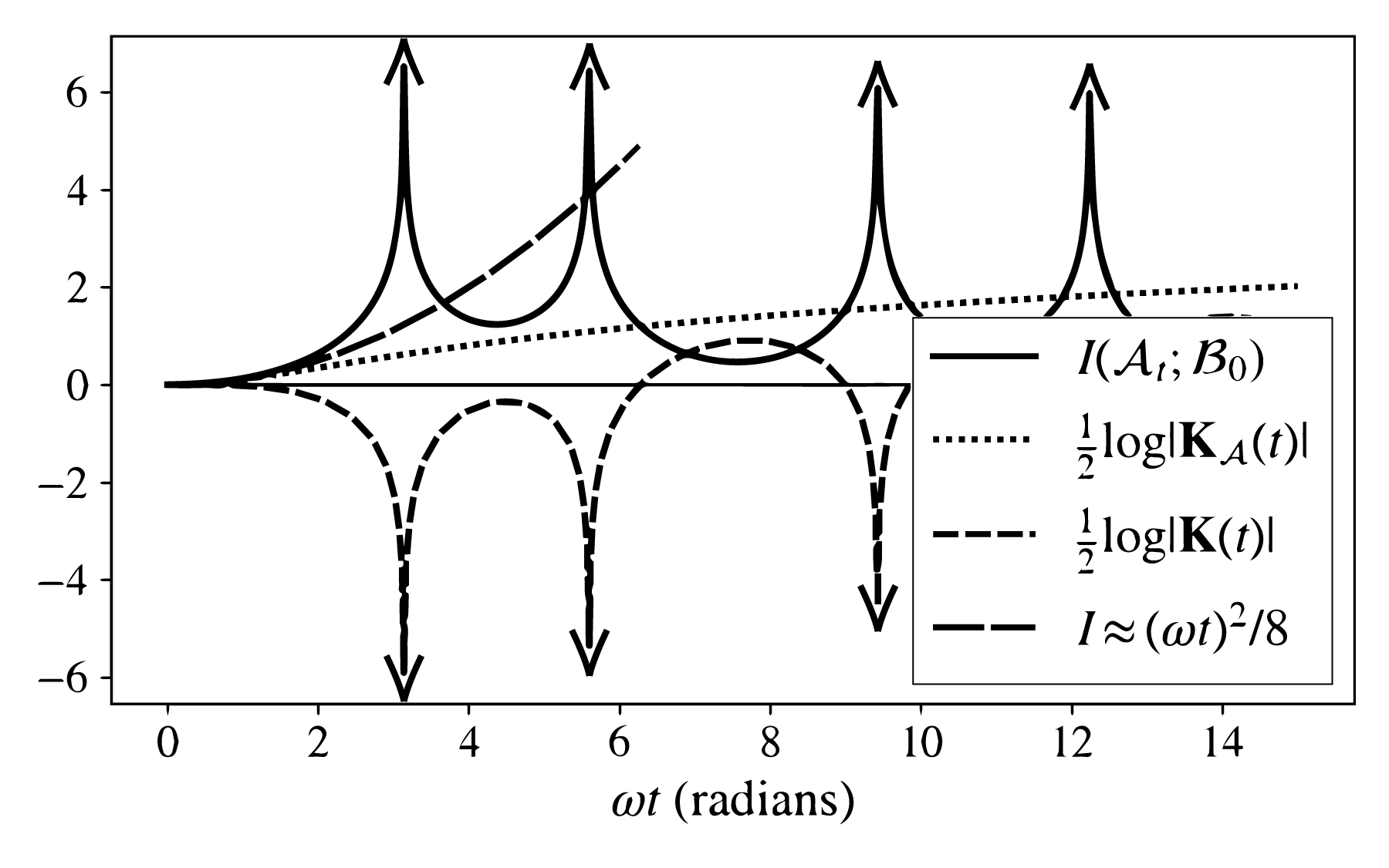
Figure 2: Determinants and Mutual Information: Shown are the log-determinants of the full covariance, ${\bf K}_{{\cal A}{\cal B}}(t)$, and that of ${\cal A}$ system, ${\bf K}_{\cal A}(t)$, as well as the mutual information, $I(\mbox{\boldmath${\cal A}$}_{t};\mbox{\boldmath${\cal B}$}_{0})$. Parameters are set so that ${\bf K}_{\cal A}(0)={\bf K}_{\cal B}(0)=\mathbf{1}_{2}$. We also show our quadratic approximation to $I(\mbox{\boldmath${\cal A}$}_{t};\mbox{\boldmath${\cal B}$}_{0})$, valid for $\omega t\ll\pi$. Arrows indicate divergence toward $\pm\infty$

III-B Comparison with the general result for small $t$

We have considered the mutual information between the state $\mbox{\boldmath${\cal A}$}_{t}$ and the state $\mbox{\boldmath${\cal B}$}_{0}$. We would like to compare this to our result in equation (11), the information flow between a particle and the force acting on it in a small time interval. To that end, we consider the case when $t\ll 1/\omega$ in equation (19). In this limit, ${\bf L}_{t}$ and ${\bf R}_{t}$ can be approximated to first order in $t$ by,

$${\bf L}_{t}\!\approx\!\left[\!\!\begin{array}[]{cc}1&\omega t\\ -\omega t/2&1\end{array}\!\!\right],\,\,\,\,\,{\bf R}_{t}\!\approx\!\left[\!\!\begin{array}[]{cc}0&0\\ \omega t/2&0\end{array}\!\!\right].$$

Making use of this approximation, we can compute the determinant of ${\bf K}_{\cal A}(t)$ to leading order in $t$:

$$|{\bf K}_{\cal A}(t)|\approx|{\bf K}_{\cal A}(0)|\left(1+\left(1+\frac{\sigma_{X_{{\cal A}_{0}}}^{2}\sigma_{X_{{\cal B}_{0}}}^{2}}{4|{\bf K}_{\cal A}(0)|}\right)(\omega t)^{2}\right),$$

assuming $|{\bf K}_{\cal A}(0)|\neq 0$, where $\sigma_{X_{{\cal A}_{0}}}^{2}$ and $\sigma_{X_{{\cal B}_{0}}}^{2}$ are the initial position variances of particles ${\cal A}$ and ${\cal B}$, respectively. Similarly, the determinant of ${\bf K}_{{\cal A}{\cal B}}(t)$ can be written,

$$|{\bf K}_{{\cal A}{\cal B}}(t)|\approx|{\bf K}_{\cal A}(0)|\hskip 2.84544pt|{\bf K}_{\cal B}(0)|\hskip 2.84544pt(1+(\omega t)^{2})$$

to leading order in $t$. Combining these, we can compute the mutual information to first order ($t\ll 1/\omega$):

$$I(\mbox{\boldmath${\cal A}$}_{t};\mbox{\boldmath${\cal B}$}_{0})\approx\frac{1}{8}\frac{\sigma_{X_{{\cal A}_{0}}}^{2}\sigma_{X_{{\cal B}_{0}}}^{2}}{|{\bf K}_{\cal A}(0)|}(\omega t)^{2}$$ (21)

which is analogous to the $t^{2}$ term in equation (10). Without further assumptions on the power exchanged between ${\cal A}$ and ${\cal B}$ in a time interval $[0,t]$, the time derivative of equation (21) vanishes as $t\rightarrow 0$. On the other hand, if we impose an average power exchange constraint on $[0,t]$ as we did in equation (5), we can derive a condition on $\sigma_{X_{{\cal B}_{0}}}^{2}$ in terms of the average power $\mathcal{P}_{0}$ on $[0,t]$, and the initial ${\cal A}$ position and velocity variances, $\sigma_{X_{{\cal A}_{0}}}^{2}$ and $\sigma_{V_{{\cal A}_{0}}}^{2}$:

$$\sigma_{X_{B_{0}}}^{2}=\frac{2m\mathcal{P}_{0}}{k^{2}t}+2\sigma_{V_{{\cal A}_{0}}}^{2}-\sigma_{X_{{\cal A}_{0}}}^{2}$$ (22)

Equation (22) can be derived from equation (8) with $g_{0}=k$, $\sigma_{V_{0}}^{2}=\omega^{2}\sigma_{V_{A_{0}}}^{2}=2k\sigma_{V_{A_{0}}}^{2}/m$ and $\mathbb{E}[F_{0}^{2}]=k^{2}(\sigma_{X_{A_{0}}}^{2}+\sigma_{X_{B_{0}}}^{2})$. And as in equation (4), we’ll assume that the initial ${\cal A}$ velocity is related to an energy scale $\mathcal{E}_{0}$ by,

$$\sigma_{V_{{\cal A}_{0}}}^{2}=\frac{\mathcal{E}_{0}}{k}$$

Note that $\sigma_{V_{{\cal A}_{0}}}^{2}$ has dimensions of length squared, owing to our definition of $V_{{\cal A}_{0}}$. Assuming independence between the initial position and velocity of the ${\cal A}$ particle, we can write the mutual information from equation (21), subject to equation (22), as,

$$I(\mbox{\boldmath${\cal A}$}_{t};\mbox{\boldmath${\cal B}$}_{0})\approx\frac{1}{4}\frac{(kt)^{2}}{m\mathcal{E}_{0}}\left(\frac{2m\mathcal{P}_{0}}{k^{2}t}+\frac{2\mathcal{E}_{0}}{k}-\sigma_{X_{{\cal A}_{0}}}^{2}\right)$$

Differentiating w.r.t. time and setting $t\rightarrow 0$, we have the maximum rate $R_{{\cal A}\leftrightarrow{\cal B}}$, that information can be passed from ${\cal B}$ to ${\cal A}$,

$$\boxed{R_{{\cal A}\leftrightarrow{\cal B}}=\frac{1}{2}\left(\frac{\mathcal{P}_{0}}{\mathcal{E}_{0}}\right)}$$ (23)

analogous to the first term in equation (11). Evidently the latter log term in equation (11) is a feature of the mutual information between a state and a force, rather than between states as we show here.

IV Discussion & Conclusion

We think our approach to the question of classical information exchange between particles has uncovered a previously unexplored relationship. Namely, we find that the information flow rate scales with $\mathcal{P}_{0}\big{/}\mathcal{E}_{0}$, whether that’s the rate of mutual information gain between particle states (equation (23)), or between states and an external force (equation (11)). In the case of two particles interacting through a springlike potential, we found that the small time approximation is consistent with the more general result, quantifying the rate of information exchange between a particle and a force from its environment.

Our springlike example also shows us the mutual information for times beyond this small $t$ window, and we found that the mutual information spikes to infinity periodically. We argued that this corresponds to one particle’s state periodically encoding a single real degree of freedom associated with the other particle—an artifact of classical physics, in which the state is a point in continuous phase space. This result effectively extends classic results on observability (in regards to the observability of one particle’s state given the other) to incorporate an information theoretic measure quantifying when a state is, at least partially, observable.

This dependence on $\mathcal{P}_{0}/\mathcal{E}_{0}$ is appealing. When more energy flows between a particle and its environment in a given amount of time, there is the potential to encode more information regarding the environment’s state. We also see that when the measuring particle’s initial energy, $\mathcal{E}_{0}$, is relatively low, this particle can encode more about the environment in a given time interval. Essentially, the change in the measuring particle’s state is more substantial in this case. Whereas, when $\mathcal{E}_{0}$ is relatively large, small energy exchanges with the environment contribute less to changes in the particle state. This is the limit of a weakly coupled environment, and is consistent with our intuition that there should be minimal information exchange as well.

We emphasize that equations (11) and (23) represent maximum information flow rates, subject to power and energy constraints. That is, the $t$ dependence in equations (9) and (22), which allowed the rate to survive the $t\rightarrow 0$ limit, result from asking what is the maximum rate that information can be transmitted—either between a state and a force (section II) or between states (section III), subject to the energy and power constraints, assuming also that the “noise,” represented by the uncertainty in the initial state of the system ($(X_{0},V_{0})$ in section II, or $\mbox{\boldmath${\cal B}$}_{0}$ in section III), is least informative, or maximally confounding. As $t\rightarrow 0$, this requires an infinite force variance in an infinitesimal time, in order for there to be non-zero information flow. In contrast, a random force with a fixed variance, independent of the timescale $t$, does not transmit any information in the limit as $t\rightarrow 0$. Evidently, the mutual information accumulated on $[0,t]$ scales like $t^{2}$, so that the rate vanishes unless the force variance scales like $\sim 1/t$, balancing the $t\rightarrow 0$ limit. As we have seen, this scaling naturally occurs when there is a constraint on the average power $\mathcal{P}_{0}$ over the interval $[0,t]$, with $\mathcal{P}_{0}$ dependent on the statistics of the initial state configuration.

We have also seen that the average power $\mathcal{P}_{0}$ scales with the coupling between system and environment. And so our work also suggests a novel interpretation of the coupling constant as a characteristic rate at which information is transmitted between subsystems. We found (equation (21)) that the mutual information is proportional to the spring constant $k$, for instance, without any additional assumptions. and we suspect that this is a generic feature of information exchange between physical systems.

References

- [1] C. Shannon, “The bandwagon (edtl.),” IRE Transactions on Information Theory, vol. 2, no. 1, pp. 3–3, 1956.
- [2] L. Brillouin, Science and Information Theory. Academic Press, 1962.
- [3] M. Planck, “Ueber das gesetz der energieverteilung im normalspectrum,” Annalen der Physik, vol. 309, no. 3, pp. 553–563, 1901. [Online]. Available: https://onlinelibrary.wiley.com/doi/abs/10.1002/andp.19013090310
- [4] ——, The Theory of Heat Radiation, ser. Dover Books on Physics Series. Dover Publications, 1991 (originally published 1914). [Online]. Available: https://books.google.com/books?id=UnGPVwLybcEC
- [5] L. Szilard, “On the decrease of entropy in a thermodynamic system by the intervention of intelligent beings,” Behavioral Science, vol. 9, no. 4, pp. 301–310, 1964. [Online]. Available: https://onlinelibrary.wiley.com/doi/abs/10.1002/bs.3830090402
- [6] J. v. Neumann, “Thermodynamik quantenmechanischer gesamtheiten,” Nachrichten von der Gesellschaft der Wissenschaften zu Göttingen, Mathematisch-Physikalische Klasse, vol. 1927, pp. 273–291, 1927. [Online]. Available: http://eudml.org/doc/59231
- [7] A. Duncan, “Von neumann’s 1927 trilogy on the foundations of quantum mechanics. annotated translations,” 2024. [Online]. Available: https://arxiv.org/abs/2406.02149
- [8] R. Landauer, “Irreversibility and heat generation in the computing process,” IBM Journal of Research and Development, vol. 5, no. 3, pp. 183–191, 1961.
- [9] C. H. Bennett, “The thermodynamics of computation—a review,” International Journal of Theoretical Physics, vol. 21, pp. 905–940, 1982. [Online]. Available: https://api.semanticscholar.org/CorpusID:17471991
- [10] ——, “Notes on landauer’s principle, reversible computation and maxwell’s demon,” 2003. [Online]. Available: https://arxiv.org/abs/physics/0210005
- [11] H. C. V. Baeyer, Warmth Disperses and Time Passes: The History of Heat. Random House Publishing Group, 1999.
- [12] M. Smoluchowski, “Experimentell nachweisbare, der üblichen thermodynamik widersprechende molekularphänomene,” Physikalische Zeitschrift, vol. 13, pp. 1069–1080, 1912.
- [13] R. P. Feynman, R. B. Leighton, and M. Sands, “The feynman lectures on physics, volume 1,” in The Feynman Lectures on Physics, Volume 1, R. P. Feynman, R. B. Leighton, and M. Sands, Eds. Reading, MA: Addison-Wesley, 1963, ch. 46.
- [14] J. M. R. Parrando, J. M. Horowitz, and T. Sagawa, “Thermodynamics of information,” Nature Physics, vol. 11, 02 2015. [Online]. Available: https://doi.org/10.1038/nphys3230
- [15] J. Preskill, “Quantum computing in the nisq era and beyond,” Quantum, vol. 2, p. 79, Aug. 2018. [Online]. Available: http://dx.doi.org/10.22331/q-2018-08-06-79
- [16] T. Cover and J. Thomas, Elements of Information Theory. Wiley-Interscience, 1991.