From non-equilibrium Green functions to Lattice Wigner: A toy model for quantum nanofluidics simulations

Abstract

Recent experiments of fluid transport in nano-channels have shown evidence of a dramatic reduction of friction due to the coupling between charge-fluctuations in polar fluids and electronic excitations in graphene solids, a phenomenon dubbed ”negative quantum friction”. In this paper, we present a semi-classical mesoscale Boltzmann-Wigner lattice kinetic model of quantum-nanoscale transport and perform a numerical study of the effects of the quantum interactions on the evolution of a one-dimensional nano-fluid subject to a periodic external potential. It is shown that the effects of quantum fluctuations become visible once the quantum length scale (Fermi wavelength) of the quasiparticles becomes comparable to the wavelength of the external potential. Under such conditions, quantum fluctuations are mostly felt on the odd kinetic moments, while the even ones remain nearly unaffected because they are ”protected” by thermal fluctuations. It is hoped that the present Boltzmann-Wigner lattice model and extensions thereof may offer a useful tool for the computer simulation of quantum-nanofluidic transport phenomena.

I Introduction

In the last three decades the Lattice Boltzmann (LB) method has offered a powerful bridge between the atomistic and macroscopic description of flowing matter, with a broad spectrum of applications across many regimes and scales of motion succi2018lattice ; benzi_phys_rep . Although the LB formalism extends to the quantum SUCCI1993327 and relativistic GABBANA20201 realms, its overwhelming body of application is focussed on classical physics, most notably complex fluids and soft matter physrep .

However, the relentless progress of nanotechnology is exposing a growing set of problems whereby quantum phenomena need to be explicitly accounted for, a paradigmatic example being the water flow in carbon nanotubes gao2017nanofluidics . Recently, it has been surmised that quantum interfacial effects in ionic fluids may contribute a sizeable reduction of the drag experienced by water molecules in the proximity of graphene confining walls, a phenomenon called negative quantum friction bocquet1 ; bocquet2 . Such quantum interfacial effects should in principle be treated by ab-initio quantum statistical mechanics methods, such as the non-equilibrium Green function (NEGF) techniques. However, due to its steep computational cost, NEGF is usually replaced by quantum extensions of molecular dynamics wang2009molecular . Even so, reaching to spatial and especially temporal scales of experimental relevance remains a major challenge. There is therefore scope for further coarse-graining, a task at which Lattice Boltzmann has proved very efficient, especially for soft flowing matter applications.

In this paper, we develop a mathematical framework taking from NEGF to LB, and most notably to high-order LB schemes capable of capturing the interplay between classical and quantum non-equilibrium fluctuations, which lies at the heart of quantum nano-fluidic transport, including negative quantum friction effects. More specifically, a high order one-dimensional LB method with third order quantum forcing terms is used to model the evolution of a nano-fluid in the presence of an external periodic potential. Our results suggest that, if the length scale of the quantum force is comparable with that of the external potential, quantum fluctuations are found to disturb odd moments (i.e. current and energy flux) of the distribution functions, whereas such moments are screend from quantum effects if the length scale of the potential is larger. On the contrary, even moments are generally shielded by thermal fluctuations, which prevail over quantum ones.

The paper is organized as follows. In section II we shortly recap the NEGF formalism and its link to the Wigner equation. Sections III and IV are dedicated to discussing the derivation of a high order LB method from the Wigner equation, while section V highlights the application of the method to the realistic case of a hydronic current drive bocquet1 ; bocquet2 . Finally, in section VI we describe the implementation of the one-dimensional LB model with quantum forces and in section VII we present the numerical results, where we study the effect of such forces on the evolution of the power moments of the distribution functions subject to a periodic potential. The main findings and conclusions are summarized in the final section.

II The non-equilibrium Green function

Following Refs. kadanoff ; rammer , we start from a quantum many-body system described by the quantum wavefunction operator $\Psi(x,t)$. The NEGF formalism is based on the Green function associated with the particle generation and destruction operators $\hat{\Psi}$ and $\hat{\Psi}^{+}$

$$G(1,2)=<\hat{\Psi}(1)\hat{\Psi}^{+}(2)>,$$ (1)

where $1$ and $2$ denote two distinct positions in four-dimensional spacetime $({\bf x},t)$ and subscript $-$ denotes the anticommutator and brackets denote ensemble averaging over a set of quantum configurations.

By setting ${\bf x}=({\bf x}_{1}+{\bf x}_{2})/2$, ${\bf r}=({\bf x}_{1}-{\bf x}_{2})/2$, $t=(t_{1}+t_{2})/2$ and $s=(t_{2}-t_{1})$ and taking the Fourier-transform, we obtain the associated Wigner function describing the distribution of quasiparticles in eight-dimensional phase-spacetime $({\bf x},{\bf p},t,E)$ wig_physrep

$$W({\bf x},t;{\bf p},E)=\int e^{-i({\bf p}\cdot{\bf r}-Es)/\hbar}G({\bf x},{\bf r};t,s)d{\bf r}ds.$$ (2)

By assuming weak interactions, which means that the quasi-particles obey the one-valued dispersion relation $E=E({\bf p})$, and integrating upon the energy variable, the Wigner equation read as follows

$$\partial_{t}W+{\bf v}\cdot\nabla_{x}W+\Theta({\bf F}\cdot\nabla_{p}W)=C,$$ (3)

where ${\bf v}={\bf p}/m$ (being $m$ the mass of the quasiparticle and ${\bf p}$ its momentum) and $C$ is a collision term resulting from the scattering processes between the quasiparticles. In the above $\Theta$ denotes a non-local functional in energy-momentum space resulting from quantum interference effects. In explicit form

$$\Theta=\sum_{k}\left(\frac{\hbar}{2i}\right)^{|k|}\frac{1}{k!}F_{k}\partial_{p}^{k},$$ (4)

where $F_{k}=-\partial_{x}^{k}U$ lat_wig , $U$ being the one-body effective potential. The Wigner function bears a close resemblance to a classical probability distribution function, in that its kinetic moments can be associated to the quasiparticle density and current, in close analogy with classical hydrodynamics. This property is key to establish a consistent bridge with the Boltzmann equation. However, its quantum nature is reflected by the fact that $W$ is a pseudo-probability distribution which can take both signs as a result of quantum interference wig_physrep .

Mathematically, this is due to the higher order derivatives in momentum space, which probe higher order spatial derivatives of the potential. Since these derivatives in the streaming term scale like odd powers of the quantum Knudsen number

$$q=\lambda_{F}/\delta,$$ (5)

quantum interference effects are responsible for the non-positivity of the Wigner function. Eq.(5) is the analogue of the Knudsen number $Kn=\lambda/\delta$, where the molecular mean free path $\lambda$ is replaced by the Fermi wavelength $\lambda_{F}=\frac{\hbar}{mv_{F}}$ (being $\hbar$ the reduced Planck constant and $v_{F}$ the Fermi speed) and $\delta$ is the typical lengthscale. Note that for quadratic potentials, the Wigner function recovers positive-definiteness and becomes fully classical, hence quantum effects are exposed by third order spatial derivatives onward.

III From NEGF to Boltzmann and high-order Lattice Boltzmann

For the homogeneous case, close to equilibrium, the dependence on ${\bf x}$ and $t$ of the Wigner function drops out. However, since we shall be dealing with quantum non-equilibrium transport phenomena, such an assumption is not justified. A Boltzmann-like equation can be derived under two major assumptions. First, the heterogeneity must be weak at the quantum scale, which is determined by the Fermi wavelength $\lambda_{F}$. Formally

$$q\ll 1,$$ (6)

which means that at the transport scale (set by $\delta$), the quantum excitations (quasiparticles) are localized, hence they can be treated as quasi classical particles.

The second assumption is that quantum excitations should be weakly interacting, meaning that their self-energy must be small as compared to classical kinetic energy $k_{B}T$ (where $k_{B}$ is the Boltzmann constant and $T$ is the temperature). Formally,

$$Fr=\frac{F\delta}{k_{B}T}\ll 1,$$ (7)

where $Fr$ is the Froude number and $F=-\nabla U$, $U(x,t)$ is the self-interaction potential, i.e. the potential energy acquired by a representative quasiparticle as a result of the interaction with all other quasiparticles. The weak-interaction regime $Fr\ll 1$ permits to associate a single-valued dispersion relation to the quantum excitations, i.e. $\omega=\omega(k)$ and $\gamma=\gamma(k)$, where $k=p/\hbar$ is the wavenumber and $\omega$ and $\gamma$ are the real and imaginary part of the complex wave-frequency. The former controls phase changes (propagation) and the latter amplitude changes (decay/stability). Under such condition the Wigner distribution can be expressed in the so called in-shell representation

$$W({\bf x},{\bf p},t,E)=f({\bf x},{\bf p},t)\delta[E-E({\bf p})],$$ (8)

so that the energy-dependence can be integrated out to yield a Boltzmann equation in six-dimensional phase-space plus time

$$\partial_{t}f+{\bf v}\cdot\nabla_{x}f+{\bf F}\cdot\nabla_{p}f=C(f,f)$$ (9)

where $C(f,f)$ is a semiclassical collision operator. In the sequel it proves expedient to replace $C$ with the corresponding single-relaxation time expression bgk

$$C=\frac{f-f^{eq}}{\tau},$$ (10)

where $f^{eq}$ is a Bose-Einstein or Fermi-Dirac local equilibrium for bosons and fermions and $\tau$ is the relaxation time.

With the Boltzmann equation at hand, the route to LB follows the standard protocol, with the important proviso that high-order lattices (HOL) are no luxury, but play a vital role instead. To this purpose let us reminds that in the theory of classical LB, HOL are usually employed to go beyond the hydrodynamic regime and describe strong non-equilibrium effects associated with non-negligible Knudsen numbers, i.e $Kn\gg 1$.

For quantum nanofluidics, there are two additional motivations: first, quantum local equilibria demand energy conservation, hence they need to be formulated on lattices extending beyond the first Brillouin region coelho2014lattice . Second, as discussed earlier on, in the presence of quantum interference, higher order derivatives in momentum space need to be accounted for, which again commends the resort to HOL.

IV Quantum interference and High-Order LB

The former aspect is discussed in full detail in coelho2014lattice , hence in the following we focus on the latter. Let us consider, for example, the third order term in one spatial dimension for simplicity, i.e. $F_{3}(x)\partial_{p}^{3}f$ where $p=p_{x}$. With reference to a generic microscopic property $\phi(p)$, the change per unit time of the macroscopic moment $\Phi_{3}(x)=\int\phi(p)f(x,p)dp$ due to the third order force is given by

$$\dot{\Phi}_{3}(x)=F_{3}(x)\int\phi(p)\partial_{p}^{3}f(x,p)dp.$$

On the assumption that all boundary contributions vanish at infinity in momentum spaces, repeated integration by parts delivers

$$\dot{\Phi}_{3}(x)=F_{3}(x)\int f(x,p)\partial_{p}^{3}\phi(p)dp,$$ (11)

which gives zero for moments below third order. However, microscopic quantities of order three (i.e. the skewness) couple to the zero-th order moment, which is the fluid density. If, for instance, $\phi(p)=p^{3}/6$, we obtain $\dot{\Phi}_{3}(x)=F_{3}(x)n(x)$; likewise, $\phi(p)=p^{4}/24$ contributes $\dot{\Phi}_{3}(x)=F_{3}(x)J$ and so on. This shows a long-range coupling in momentum space as a result of quantum interference, whence the need of high-order lattices. A detailed list of 2D lattices (whose implementation is challenging but conceptually straightforward) with up to sixteenth order isotropy can be found in sbragaglia2007generalized .

Indeed, previous numerical simulations have shown that the use of HOL leads to more accurate results in the case of anharmonic (fourth-order) potentials, confirming that kinetic moments of order above three do couple to the hydrodynamic sector solorzano2018lattice ; brewer2016lattice . This is because third order derivatives in momentum space, as applied to an Hermite mode of order $n$, excites modes of order $n+3$ in the Hermite ladder.

V Prospective application to hydronic current drive

In this section we discuss the relevant regimes for hydronic current drive nanodevices succi2024keldysh . To convey a concrete idea of a typical application scenario, let us consider a fluid of water molecules flowing in a nano-channel, say a carbon nanotube, confined by carbon walls, either graphite or graphene bocquet1 ; bocquet2 .

Water is driven by an external pressure gradient and dissipates energy and momentum on the solid walls. However, at variance with the classical picture, whereby such dissipation is due to classical interaction of the water molecules with solid molecules at the wall, new interfacial interactions need to be considered. In particular, the nanoscale fluctuations of the water molecules give rise to corresponding nanoscale fluctuations of the molecular charge (dubbed hydrons), which couple to electronic degrees of freedom in the solid wall via screened Coulomb interactions. At the same time, classical mechanical collisions of the water molecules with the solid walls generate phonon excitations in the solid. Due to phonon-electron scattering, these two mechanisms induce a net motion of both excitations, namely a ”phonon wind” and an ”electron wind”, which are ultimately stabilized by momentum and energy dissipation on the solid crystal, thus closing the energy balance.

Ab-initio analysis based on the quantum non-equilibrium Keldysh formalism predicts that the interaction between water and hydrons in the liquid, electrons and phonons in the solid, leads to a broad variety of energy exchange patterns between the flowing water and the electron-photon ”fluids” in the solid, including the possibility that the electrons may return energy and momentum back to the liquid, thereby leading to a reduction of the friction experienced by water, a mechanism dubbed ”negative quantum friction” bocquet1 ; bocquet2 .

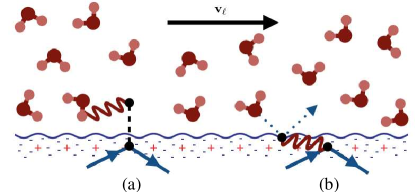
Figure 1: Two different mechanisms driving the electronic current: (a) water molecules subject to charged fluctuations (hydrons, red wavy line) transferring momentum to the electrons (black dots) in the solid through Coulomb interaction; (b) phonons (wavy line), excited by water molecules collisions, drive electrons in the solid. The figure is adapted from Ref.bocquet2 .

Such quantum effects can be estimated in terms of the quantum Knudsen number $q$ (defined in Eq.5), where the spatial scale of the hydrodynamic fields $\delta$ is assumed comparable to the lengthscale of the interaction potential. The quantum Knudsen number controls the strength of the quantum force versus the classical one, namely

$$\frac{F_{3}\partial_{p}^{3}f}{F_{1}\partial_{p}f}\sim q^{2},$$ (12)

where we have taken $\partial_{x}\sim\delta^{-1}$ and $\partial_{p}\sim 1/(mv_{F})$. Another useful dimensionless group is the ”quantumness”, hereby defined as the ratio of the Fermi wavelength to a characteristic mean free path

$$\mathcal{Q}\equiv\lambda_{F}/\lambda.$$ (13)

By definition, the $q$ and $\mathcal{Q}$ are related via the classical mean free path as $q=\mathcal{Q}{Kn}$. This shows that the condition $\mathcal{Q}>1$ indicates that we are dealing with quantum fluids. To be noted at variance with $q$, which is flow-dependent, that the quantumness is inherently a fluid property. Also to be appreciated that it displays an upper bound dictated by the celebrated AdS-CFT minimum viscosity bound kovtun ; trachenko , which states that any fluid should fulfill the following inequality

$$\frac{\eta}{s}\geq\frac{1}{4\pi}\frac{\hbar}{k_{B}},$$ (14)

where $\eta$ is the dynamic viscosity of the fluid and $s$ is the entropy density. The above inequality is nearly saturated by strongly interacting fluids, such as quark-gluon plasmas, whereas ordinary fluids lie about two or more orders of magnitude above. By recasting Eq.(14) in terms of the ”quantumness”, we readily obtain $\mathcal{Q}\leq 4\pi$, where we have taken the entropy per particle of order unity.

Next we consider typical values for a quanto-nanofluidic application, with reference to a nanotube of diameter $D=10$ nm and length $L=100$ nm, with solid wall thickness $a=1$ nm. The electron Fermi wavelength is $\lambda_{F}=h/\sqrt{mE_{f}}\sim 2.5$ nm, where we have taken $m=m_{e}/10$ for the effective electron mass in graphene and $E_{F}\simeq 100$ meV bocquet1 . Assuming longitudinal propagation of the electrons and a transport scale $\delta\sim 10$nm, we have $q\sim 0.25$. This shows that the electron mean free path is comparable with the Fermi wavelength, hence the electronic excitations can be treated semi-classically. We note that in our case, the value of the quantumness $\mathcal{Q}\sim 1$ points indeed to a strongly interacting fluid, but still consistent with the AdS-CFT bound.

VI The D1Q5 model with quantum forces

Here we describe a one-dimensional lattice Boltzmann method to study dynamics of the first five moments of the Wigner distribution function. We consider a D1Q5 lattice consisting of five discrete speeds $c_{i_{x}}=c_{i}$, where $c_{i}=\frac{\Delta x}{\Delta t}$ (with $i=0,1,2,3,4$), $\Delta x$ is the lattice step and $\Delta t$ is the time step, with modulus $c_{0}=0$, $c_{1}=+1$, $c_{2}=-1$, $c_{3}=+2$, $c_{4}=-2$ (see Fig.2).

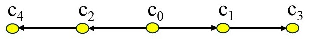
Figure 2: D1Q5 lattice Boltzmann scheme. Black arrows indicate lattice speeds $c_{i}$ where $i=0,1,2,3,4$.

A set of distribution functions $f_{i}(x,t)$, defined on each site $x$ and time $t$, evolves following a discrete Boltzmann equation succi2018lattice

$$f_{i}(x+c_{i}\Delta t,t+\Delta t)=(1-\omega)f_{i}(x,t)+\omega f_{i}^{eq}(x,t)+S_{i}(x,t),$$ (15)

where $\omega$ is a frequency tuning the relaxation towards the equilibrium and controlling the fluid viscosity $\nu=(1/\omega-1/2)c_{s}^{2}\Delta t$ (with $c_{s}$ lattice sound speed and $c_{s}^{2}=1$), $f_{i}^{eq}$ are the local equilibrium populations and $S_{i}$ are the source terms succi2018lattice . Following common practice in LB theory succi2018lattice ; halim , the former are computed as a second-order Taylor expansion in the fluid velocity $u$ (where $u=u_{x}$) at low Mach number

$$f_{i}^{eq}=w_{i}\rho\left[1+\frac{uc}{c^{2}_{s}}+\frac{u^{2}(c_{i}c_{i}-c^{2}_{s})}{2c_{s}^{4}}\right],$$ (16)

where $\rho$ is the fluid density and $w_{i}$ is a set of weights with values $w_{0}=\frac{6}{12}$, $w_{1}=w_{2}=\frac{2}{12}$ and $w_{3}=w_{4}=\frac{1}{12}$. Also, the fluid density $\rho$ and the fluid momentum $\rho u$ can be computed from the moments of the distributions $f_{i}$ as $\rho=\sum_{i}f_{i}$ and $\rho u=\sum_{i}f_{i}c_{i}$.

Note that the actual populations $f_{i}$ can be written in terms of the kinetic moments $M_{i}$ as follows

$$f_{i}(x,t)=w_{i}\sum_{k=0}^{4}M_{k}(x,t)V_{i}^{k},$$ (17)

where $V_{i}^{k}$ is a set of orthogonal eigenvectors

$$V^{0}_{i}=1_{i}=[1,1,1,1,1],$$ (18)

$$V^{1}_{i}=c_{i}=[0,1,-1,2,-2],$$ (19)

$$V^{2}_{i}=c_{i}^{2}-c_{s}^{2}=[-1,0,0,3,3],$$ (20)

$$V^{3}_{i}=c_{i}^{3}-3c_{i}c_{s}^{2}=[0,-2,2,2,-2],$$ (21)

$$V^{4}_{i}=c_{i}^{4}-4c_{i}^{2}c_{s}^{2}+c_{s}^{4}=[1,-2,-2,1,1].$$ (22)

The kinetic moments are thus given by

$$M_{k}(x,t)=\sum_{i=0}^{4}f_{i}(x,t)V_{i}^{k},$$ (23)

which are used to systematically derive the equations of motion and the forcing terms.

VI.1 Equations of motion

By multiplying Eq.(15) by $1,c_{i},c_{i}^{2},c_{i}^{3},c_{i}^{4}$ and summing up, the equations of motion take the following form

$$\partial_{t}M_{0}+\partial_{x}M_{1}=0,$$ (24)

$$\partial_{t}M_{1}+\partial_{x}M_{2}=S_{1}^{cl},$$ (25)

$$\partial_{t}M_{2}+\partial_{x}M_{3}=-\omega(M_{2}-M_{2}^{eq})+S_{2}^{cl},$$ (26)

$$\partial_{t}M_{3}+\partial_{x}M_{4}=-\omega(M_{3}-M_{3}^{eq})+S_{3}^{cl}+S_{3}^{q},$$ (27)

$$\partial_{t}M_{4}+\partial_{x}M_{5}=-\omega(M_{4}-M_{4}^{eq})+S_{4}^{cl}+S_{4}^{q},$$ (28)

where $S_{i}^{cl,q}$ are the classical and quantum forces, whose computation is presented in the next subsection.

Rather than studying the physics of the kinetic moments $M_{k}$, we prefer monitoring the effect of the quantum force on the power moments $P_{k}$, which are given by

$$P_{k}=\sum_{i=0}^{4}f_{i}c_{i}^{k},\;\;k=0,1,2,3,4.$$ (29)

Indeed, besides carrying a direct physical interpretation, these moments allow for an easier analysis of the origin of the quantum effects which are expected to play a role in the absence of thermal fluctuations. In this respect, one can easily prove that $P_{0}=\rho$, $P_{1}=\rho(u+\theta_{1})$, $P_{2}=\rho(u^{2}+\theta_{2})$, $P_{3}=\rho(u^{3}+u\theta_{2}+\theta_{3})$ and $P_{4}=\rho(u^{4}+6u^{2}\theta_{2}+\theta_{4})$, where $\rho\theta_{p}=\sum_{i=1}^{4}f_{i}(c_{i}-u)^{p}$, being $\theta_{p}$ the correlator.

Note that the odd correlators $\theta_{1}$ and $\theta_{3}$ vanish at equilibrium, while the even correlators do not, since they carry the contribution of thermal fluctuations, namely $\theta_{2}^{eq}=c_{s}^{2}$ is the square of the thermal speed and $\theta_{4}^{eq}=3c_{s}^{4}$ is the flatness of the equilibrium distribution. These values corresponds to the central moments a Gaussian profile, where $\theta_{3}^{eq}$ is the skewness and $\theta_{4}^{eq}$ is the kurtosis. At equilibrium one has $P_{1}^{eq}=\rho u$, $P_{2}^{eq}=\rho(u^{2}+c_{s}^{2})$ and $P_{3}^{eq}=\rho u(u^{2}+c^{2}_{s})$, corresponding to the fluid current, the energy density and the energy flux density, respectively. The non-equilibrium components of the correlators are associated with non-equilibrium fluctuations driven by heterogeneity and they are responsible for irreversible transport phenomena.

VI.2 Forcing terms

Next we consider the effect of the forcing terms. For classical forces we have

$$S^{cl}(x,p,t)=-F_{1}(x)\partial_{p}f,$$ (30)

where $F_{1}(x)=-\partial_{x}U(x)$ and $U(x)$ is the external potential, while the associated moments are

$$S_{k}^{cl}(x,t)=F_{1}(x)\int H_{k}(p)\partial_{p}fdp=-F_{1}(x)\int f\partial_{p}H_{k}(p)dp,$$ (31)

where $H_{k}(p)$ is an Hermite basis in continuum velocity space. Simple integration by parts delivers $S^{cl}_{0}=0$, $S^{cl}_{1}=\rho F_{1}$, $S^{cl}_{2}=2JF_{1}$, $S^{cl}_{3}=3JuF_{1}$, $S^{cl}_{4}=4Ju^{2}F_{1}$, where $J=\rho u$. The contributions to the discrete distributions can be cast in the same form as the discrete distributions themselves, namely

$$S_{i}(x,t)=w_{i}\sum_{k=0}^{4}S_{k}(x,t)V_{i}^{k},$$ (32)

which are the source terms associated with the classical force. The same procedure applied to the quantum force

$$S^{q}(x,p,t)=-F_{3}(x)\partial_{p}^{3}fdp$$ (33)

delivers $S^{q}_{0}=0$, $S^{q}_{1}=0$, $S^{q}_{2}=0$, $S^{q}_{3}=6\rho F_{3}$, $S^{q}_{4}=24JF_{3}$, where $F_{3}(x)=-\partial_{x}^{3}V$. Note that the quantum force does not act directly upon the first three moments, namely density, current and energy, although it can affect them through the gradients of the moments of order three and four. Also, since $F_{3}(x)$ stems from a third order derivative in space of the external potential, the quantum force is most effective on the short scales. For a potential lenghtscale $\delta$, the ratio of the quantum force to the classical one scales exactly like $q^{2}$.

VII Numerical results

To inspect the effect of the quantum fluctuations, we study the relaxation of a one-dimensional fluid in the presence of an external potential.

The latter has the following periodic form

$$V(x)=-\frac{V_{0}}{k_{n}}cos(k_{n}x),$$ (34)

where $k_{n}=\frac{\pi}{L}n_{w}$ and $n_{w}$ is the wavenumber. This leads to $F_{1}(x)=V_{0}sin(k_{n}x)$ and $F_{3}(x)=-V_{0}k_{n}^{2}sin(k_{n}x)$. The simulations are initialized with an inhomogeneous density distribution following a Gaussian profile and run for approximately $10^{4}$ time steps. If not stated otherwise, we study this system for two values of $n_{w}$, i.e. $n_{w}=8$ (low frequency regime) and $n_{w}=32$ (high frequency regime), two values of $\omega$, i.e. $\omega=0.5$ and $\omega=1$, $V_{0}=10^{-4}$ and $L_{x}=128$ in the absence and presence of the quantum force $F_{3}$. Also, the lattice spacings are set to $\Delta x=1$ and $\Delta t=1$ which would approximately correspond to $1$ nm and $1$ ps in real units. This leads to a channel length of roughly $128$ nm and an experiment lasting for $\sim 10$ ns. If we take $\lambda_{F}\sim 5\Delta x$ and $\delta\sim L/n_{w}$, we have $q\sim 0.3$ for $n_{w}=8$ and $q\sim 1.25$ for $n_{w}=32$, thus quantum effects are expected to become visible at high wavenumbers.

VII.1 Low wavenumber regime

In Fig.3 we show the time evolution of the five power moments $P_{k}$ of classical and quantum distributions for $n_{w}=8$ and $\omega=1$ (setting the numerical viscosity to $\nu=0.5$), where the initial Gaussian profile of the density is centered at $L/2$ with a standard deviation $\sigma=4$. Classical profiles are obtained by setting $F_{3}=0$, while quantum ones include $F_{3}$. At $t=0$, all moments except $P_{0}$ are zero. Our results show that the first three moments, $P_{0}$, $P_{1}$ and $P_{2}$, are not affected by quantum forces to any appreciable extent, not even through gradients of higher order moments. Both classical and quantum distributions of $P_{0}$ and $P_{2}$ gradually relax towards an almost flat profile with values slightly larger than $1$ (Fig.3a), while $P_{1}$ displays a wave-like symmetric profile (Fig.3,b,c). The first moment $P_{1}$ is positive for $x<L/2$ and negative elsewhere, with fixed zeroes at the boundaries and at $L/2$ (i.e. where density gradients are constant), while maximum and minimum (corresponding to the inflection points of the density profile) gradually shift towards lower values, until the current vanishes everywhere.

Quantum effects are found to very mildly affect only the moment $P_{3}$ (see Fig.3d,f), whose quantum distribution slightly deviates from the classical one, which displays a wave-like symmetric profile overall akin to $P_{1}$. The distribution $P_{4}$ follows the typical behavior of the even moments and is basically unaffected by any quantum deviations (Fig.3e). The different response of the moments $P_{3}$ and $P_{4}$ to the quantum force depends on the fact that, for the even moments, the effect of such a force is masked by the thermal fluctuations which, on the contrary, vanish at equilibrium for the odd moments. Note also that amplitude and frequency of both distributions at late times (Fig.3g) remain essentially consistent with the values of amplitude $V_{0}$ and wavenumber $n_{w}$ set by the periodic potential $V(x)$.

Deviations from the classical distribution can be approximately quantified in terms of the percentage error $\Delta_{k}=100\times\frac{|P_{k}^{cl}-P_{k}^{q}|}{P_{k}^{cl}}$, where $P_{k}^{cl}$ and $P_{k}^{q}$ stand for classical and quantum distributions. As previously mentioned, $\Delta_{k}$ is negligible for all moments except $P_{3}$, where the highest value is found around $7\%$.

These results point towards a picture where, as long as $q$ remains below one (i.e. when $n_{w}$ is relatively low), the effect of the quantum force on the moments is basically negligible. In the next section we show that this scenario changes significantly at increasing values of $n_{w}$.

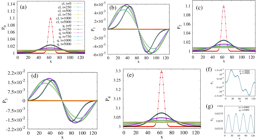
Figure 3: Power moments $P_{0}$, $P_{1}$, $P_{2}$, $P_{3}$ and $P_{4}$ at simulation time $t=0$, $250$, $500$, $750$, $1000$, $5000$ for $n_{w}=8$ and $\omega=1$. The classical (”cl”) and quantum (”q”) distributions of the first three moments (a,b,c) are basically indistinguishable. While $P_{0}$ and $P_{2}$ relax in a similar manner starting from a Gaussian profile, $P_{1}$ exhibits an intermediate wave-like behavior, which progressively flattens towards a uniform profile. The effect of the quantum force is slightly visible for $P_{3}$ where the quantum distribution barely deviates from the classical one, as highlighted in the late-time profile shown in (f). Such effects are essentially indiscernible for $P_{4}$ (e and g).

VII.2 High wavenumber regime

In Fig.4 and Fig.5 we show, for example, the time evolution of the even and odd power moments for $n_{w}=32$ and $\omega=1$. While the time behavior (Fig.4a,b,c and Fig.5a,b) is overall akin to the one observed for lower values of $n_{w}$, the effect of the quantum force is clearly visible on the profiles of all power moments (as shown in Fig.4d,e,f and Fig.5c,d). Indeed, although the quantum force enters explicitly only the moments $M_{3}$ and $M_{4}$ in Eqs.(27-28) (and thus $P_{3}$ and $P_{4}$), its effect actually conditions lower moment through spatial derivatives (for instance $\partial_{x}M_{3}$ in Eq.(26)) resulting from the hierarchical structure of the equations of motion.

In the present problem, the quantum force manifests through a change of amplitude of the distributions, which display a wave-like behavior with a well-defined frequency (set by $n_{w}$). Considering, for example, the late-time profile of $P_{4}$ in Fig.4f, the quantum force amplifies the classical signal, whose minima correspond to the maxima of the quantum distribution (leading to an apparent phase-shift effect). This happens because $F_{1}$ and $F_{3}$ carry opposite signs and different amplitudes, where $F_{1}\propto V_{0}$ and $F_{3}\propto-V_{0}k^{2}_{n}$. Lower moments generally show similar features, although maxima and minima of classical and quantum distribution are found to align (such as in $P_{0}$, $P_{1}$ and $P_{3}$) and the amplitude of the quantum signal can decrease (as in $P_{2}$). Finally, the odd moments show values of $\Delta_{k}$ considerably higher than the even ones. Specifically, we find that the highest values are $\Delta_{1}\simeq 30\%$ and $\Delta_{3}\simeq 50\%$ (a difference arising essentially because the effect of the quantum force is mitigated for lower moments), while $\Delta_{0,2,4}$ are lower than $1\%$, although not negligible.

It is also of interest to understand whether modifying the viscosity alters such a picture. In Fig.5 we show the time evolution of the power moments for $\omega=0.5$, which sets a numerical viscosity $\eta=1.5$. Note that, although $0<\omega<2$, the AdS-CFT minimum viscosity bound would impose a lower upper bound, which would be safely set at $\omega\simeq 1.5$. Once again quantum effects condition all moments, in a way overall akin to the scenario observed for the larger values of $\omega$ and with similar values of $\Delta_{k}$. Note that increasing the viscosity leads to a decrease (both in the classical and quantum distributions) of the amplitudes of the odd moments $P_{1}$ ad $P_{3}$ (corresponding to current and energy flux respectively) with respect to $\omega=1$ and to fully equilibrated (without any modulation-like effect) late-time profiles, essentially because larger values of $\eta$ entail a faster equilibration.

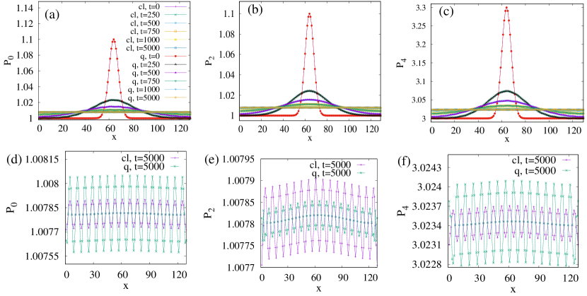
Figure 4: Even power moments $P_{0}$ (a), $P_{2}$ (b), $P_{4}$ (c) at $t=0$, $250$, $500$, $750$, $1000$, $5000$ for $n_{w}=32$ and $\omega=1$. Figures (d), (e), (f), highlight the moment profiles at $t=5000$. The time evolution is overall akin to that observed for $n_{w}=8$. However, here the quantum force generally induces an amplitude change, either larger or smaller than that of the classical profile, as shown in the late-time profiles (d,e,f). The misalignment of maxima and minima between the distributions (for example in $P_{3}$ and $P_{4}$) results from the signed amplitude of the forces, $F_{1}\propto V_{0}$ and $F_{3}\propto-V_{0}k^{2}_{n}$.

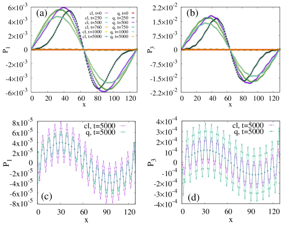
Figure 5: Odd power moments $P_{1}$ (a), $P_{3}$ (b), at $t=0$, $250$, $500$, $750$, $1000$, $5000$ for $n_{w}=32$ and $\omega=1$. Figures (d), (e), (f), highlight the moment profiles at $t=5000$. The time evolution of the distributions is similar to the one observed for lower wavenumbers, although here larger values of $n_{w}$ induce slightly wider undulations. The quantum force yields, once again, a change of amplitude with respect to the classical signal (c,d).

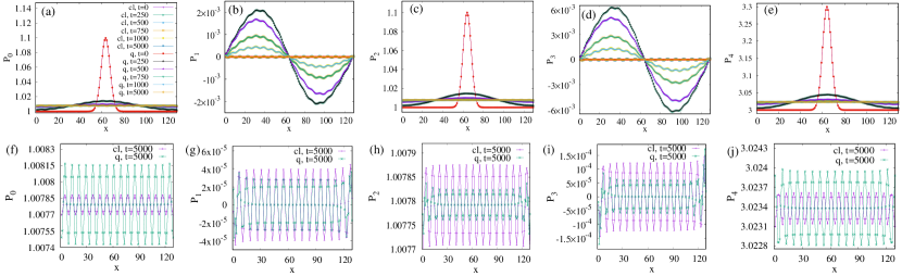
Figure 6: Power moments $P_{0}$ (a), $P_{1}$ (b), $P_{2}$ (c), $P_{3}$ (d) and $P_{4}$ (e) at $t=0$, $250$, $500$, $750$, $1000$, $5000$ for $n_{w}=32$ and $\omega=0.5$. Figures (f), (g), (h), (i) and (j) highlight the moment profiles at $t=5000$. Unlike the previous case, here lower values of $\omega$ mainly affect odd moments, which display an undulated profile with smaller amplitude. At late times, both $P_{1}$ and $P_{3}$ do not show appreciable modulations; this is because, at larger viscosity, the fluid equilibrates on a shorter time scale.

VIII Conclusions

Summarizing, we have presented a mathematical derivation of a high-order Boltzmann-Wigner lattice kinetic equation starting from non-equilibrium Green function formulation of quantum non-equilibrium transport phenomena. Simulations of a minimal D1Q5 lattice with third order quantum forcing terms for the case of a periodic potential indicate that in the semiclassical regime ($q<1$) the lowest hydrodynamic modes are well protected against quantum interference effects as long as the wavenumber $n_{w}$ (controlling the characteristic lenghtscale $\delta$) is sufficiently low. In actual practice, it is reasonable to assume that the length scale of the effective potential be significantly larger than the relevant Fermi wavelength, namely $k_{F}\delta>1$, where $k_{F}$ is the modulus of the Fermi wavevector. Of course, such an assumption needs to be checked on a case-by-case basis, but the fact remains that the lowest order moments (i.e. density and current) can only be affected by quantum interference effects on condition of strong coupling with classical non-equilibrium effects carried by the spatial gradient of the ”handshaking” moment $P_{2}$. This is indeed observed at larger values of $n_{w}$ (when $q>1$), where the presence of the quantum force generally yields a substantial change of amplitude of the classical signal. This is particularly relevant for odd moments where thermal fluctuations vanish at equilibrium, thus allowing quantum effects to emerge. It is therefore plausible to expect that the lattice Boltzmann-Wigner equation discussed in this paper may provide an efficient description of a variety of quantum-nanofluidic phenomena.

Data availability statement

The data that support the findings of this study are available from the corresponding author upon reasonable request.

Conflict of interest

The authors have no conflicts to disclose.

IX Acknowledgements

The authors are grateful to L. Bocquet, N. Kavokine and T. Kaxiras for many valuable hints and discussions. M. L. and A. T. acknowledge the support of the Italian National Group for Mathematical Physics of INdAM (GNFM-INdAM).

References

- [1] S. Succi. The lattice Boltzmann equation: for complex states of flowing matter. Oxford University Press, 2018.
- [2] R. Benzi, S. Succi, and M. Vergassola. The lattice Boltzmann equation: theory and applications. Phys. Rep., 222(3):145–197, 1992.
- [3] S. Succi and R. Benzi. Lattice Boltzmann equation for quantum mechanics. Physica D: Nonlinear Phenomena, 69(3):327–332, 1993.
- [4] A. Gabbana, D. Simeoni, S. Succi, and R. Tripiccione. Relativistic lattice Boltzmann methods: Theory and applications. Phys. Rep., 863:1–63, 2020.
- [5] A. Tiribocchi, M. Durve, M. Lauricella, A. Montessori, J. M. Tucny, and S. Succi. Lattice Boltzmann simulations for soft flowing matter. Phys. Rep., 1105:1–52, 2025.
- [6] J. Gao, Y. Feng, W. Guo, and L. Jiang. Nanofluidics in two-dimensional layered materials: inspirations from nature. Chem. Soc. Rev., 46(17):5400–5424, 2017.
- [7] N. Kavokine, M. L. Bocquet, and L. Bocquet. Fluctuation-induced quantum friction in nanoscale water flows. Nature, 602:84–90, 2022.
- [8] B. Coquinot, L. Bocquet, and N. Kavokine. Quantum feedback at the solid-liquid interface: Flow-induced electronic current and its negative contribution to friction. Phys. Rev. X, 13:011019, 2023.
- [9] J.-S. Wang, X. Ni, and J.-W. Jiang. Molecular dynamics with quantum heat baths: Application to nanoribbons and nanotubes. Phys. Rev. B, 80(22):224302, 2009.
- [10] L. P. Kadanoff and G. Baym. Quantum Statistical Mechanics: Green’s Function Methods in Equilibrium and Nonequilibrium Problems. W.A. Benjamin, 1962.
- [11] J. Rammer. Quantum Field Theory of Non-Equilibrium States. Cambridge University Press, 2007.
- [12] M. Hillery, R. F. O’Connell, M. O. Scully, and E. P. Wigner. Distribution functions in physics: Fundamentals. Physics Reports, 106(3):121–167, 1984.
- [13] S. Solórzano, M. Mendoza, S. Succi, and H. J. Herrmann. Lattice Wigner equation. Phys. Rev. E, 97:013308, 2018.
- [14] P. L. Bhatnagar, E. P. Gross, and M. Krook. A model for collision processes in gases. i. Small amplitude processes in charged and neutral one-component systems. Phys. Rev., 94:511–525, 1954.
- [15] R.C.V. Coelho, A. Ilha, M. M. Doria, R.M. Pereira, and V. Y. Aibe. Lattice boltzmann method for bosons and fermions and the fourth-order hermite polynomial expansion. Phys. Rev. E, 89(4):043302, 2014.
- [16] M. Sbragaglia, R. Benzi, L. Biferale, S. Succi, K. Sugiyama, and F. Toschi. Generalized lattice boltzmann method with multirange pseudopotential. Phys. Rev. E, 75(2):026702, 2007.
- [17] S. Solorzano, M. Mendoza, S. Succi, and H. J. Herrmann. Lattice wigner equation. Physical Review E, 97(1):013308, 2018.
- [18] J. Brewer, M. Mendoza, R. E. Young, and P. Romatschke. Lattice boltzmann simulations of a strongly interacting two-dimensional fermi gas. Physical Review A, 93(1):013618, 2016.
- [19] S. Succi and A. Montessori. Keldysh-lattice Boltzmann approach to quantum nanofluidics. arXiv preprint arXiv:2403.15768, 2024.
- [20] P. K. Kovtun, D. T. Son, and A. O. Starinets. Viscosity in strongly interacting quantum field theories from black hole physics. Phys. Rev. Lett., 94:111601, 2005.
- [21] K. Trachenko and V. V. Brazhkin. Minimal quantum viscosity from fundamental physical constants. Science Advances, 6(17):eaba3747, 2020.
- [22] T. Krüger, H. Kusumaatmaja, A. Kuzmin, O. Shardt, G. Silva, and E. M. Viggen. The Lattice Boltzmann Method: Principles and Practice. Springer International Publishing, 2017.