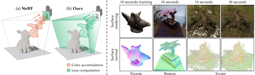
Figure 1. Our method reconstructs surfaces with the speed and robustness of NeRF-style methods. Left: In contrast to volume-based methods that minimize 2D image losses, as shown in (a), we adopt a spatio-directional radiance field loss formulation, as shown in (b). At each step, our method considers a distribution of optically independent surfaces, increasing the confidence of candidates that agree with the reference imagery. Right: A meaningful surface can be extracted at any iteration during optimization.

A Radiance Field Loss for Fast and Simple Emissive Surface Reconstruction

Abstract.

We present a fast and simple technique to convert images into an emissive surface-based scene representation. Building on existing emissive volume reconstruction algorithms, we introduce a subtle yet impactful modification of the loss function requiring changes to only a few lines of code: instead of integrating the radiance field along rays and supervising the resulting images, we project the training images into the scene to directly supervise the spatio-directional radiance field.

The primary outcome of this change is the complete removal of alpha blending and ray marching from the image formation model, instead moving these steps into the loss computation. In addition to promoting convergence to surfaces, this formulation assigns explicit semantic meaning to 2D subsets of the radiance field, turning them into well-defined emissive surfaces. We finally extract a level set from this representation, which results in a high-quality emissive surface model.

Our method retains much of the speed and quality of the baseline algorithm. For instance, a suitably modified variant of Instant NGP maintains comparable computational efficiency, while achieving an average PSNR that is only 0.1 dB lower. Most importantly, our method generates explicit surfaces in place of an exponential volume, doing so with a level of simplicity not seen in prior work.

1. Introduction

The task of reconstructing surfaces from a set of photographs has been a long-standing challenge [Moons et al., 2010]. The appeal of surface representations, aside of their natural alignment with the physical reality of objects, lies in their suitability for editing, animation and efficient rendering, which explains their near-ubiquitous use in 3D graphics applications. Unfortunately, the optimization landscape of a differentiably rendered surface tends to be non-convex and riddled with local minima. Consequently, the resulting methods are often too fragile to handle complex, real-world scenes.

This problem can be cleverly sidestepped [Mildenhall et al., 2020; Kerbl et al., 2023] by switching to a volumetric formulation of light transport. The derivative of a continuous volumetric representation is not only easier to evaluate, but it also leads to a smoother loss landscape that brings enhanced robustness and scalability. However, these improvements come at the cost of a more involved surface extraction process requiring additional heuristics, such as surface-promoting regularizers [Wang et al., 2021] or multi-stage optimization [Guédon and Lepetit, 2024].

In this work, we seek a simple and direct approach to optimize surfaces that retains the robustness and convergence speed of volumetric methods. Our proposed method builds on a simple yet powerful idea: optimizing a distribution over surfaces. Concretely, we propose projecting the training photographs into the scene and minimizing the attenuated difference between the resulting light field and the spatial-directional emission originating from the surface distribution.

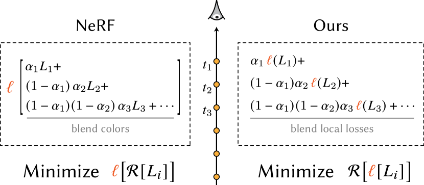
Figure 2. Comparison of the loss in volumetric optimization and our radiance field loss. We denote alpha blending by $\mathcal{R}$ and the color difference metric as ${\color[rgb]{0.94140625,0.3515625,0.140625}\ell}(L)\coloneq{\color[rgb]{0.94140625,0.3515625,0.140625}\ell}(L,L_{\text{target}})$ and drop its dependency on the target color for simplicity. Traditional volumetric reconstruction minimizes the image-space loss of blended colors. In contrast, our method minimizes a blended radiance field loss that yields a distribution of surfaces out of which a surface representation can be trivially extracted, e.g., via marching cubes.

The resulting radiance field loss considers each point along a ray as a surface candidate, individually optimized to match that ray’s pixel color, leading to the desired distribution over surfaces. One benefit is that points along a ray receive independent gradients, allowing the color or density to simultaneously increase at a point and decrease at another. This is notably different to the volumetric approach, which integrates the color along the ray prior to the loss computation (see Figure 1, left). That is, with volume reconstruction, all points along a ray receive a gradient with the same sign if their integrated color is too dark or bright, leading to correlated adjustments.

Interestingly, our proposed radiance field loss gives rise to equations remarkably similar to those of volumetric reconstruction methods (see Figure 2). In practical terms, this means that our method is simple to integrate into existing volumetric frameworks. It also means that we inherit many advantages of these prior works, without having to resort to additional heuristics to extract a surface. While we have not focused on competing with existing methods in terms of metrics, our proof of concept implementation in Instant NGP [Müller et al., 2022] consists of a few modified lines of code in the core algorithm and runs at roughly the same speed (in terms of PSNR vs. time) while producing surfaces whose PSNR is, on average, only $0.1$ dB lower than that of the volumetric approach.

2. Related work

This section reviews related work in the field of 3D surface reconstruction for novel view synthesis and tasks centered on geometric representations. Because this is such an active field, we highlight particularly salient prior works rather than attempting an exhaustive survey. As such, we only cover differentiable rendering and omit classical techniques like silhouette carving [Laurentini, 1994].

Evolving a surface

The first works on differentiable rendering embraced the high-level approach of optimizing an initial guess of a shape via gradient descent [Loper and Black, 2014], variously representing the surface using SDF level sets [Zhang et al., 2021; Vicini et al., 2022], triangle meshes [Nicolet et al., 2021], points [Chen et al., 2024b], or hybrids [Munkberg et al., 2022]. Regardless of the underlying representation, it remains challenging to achieve satisfactory results in this way: this is partly due to the complex loss landscape of an evolving surface, and partly due to the numerical difficulties of computing visibility-induced gradients [Loubet et al., 2019; Zhang et al., 2020, 2023]. Without intricate special-case handling, the optimization often fails when topological changes are required [Mehta et al., 2023], or when the surface does not overlap with the target shape [Xing et al., 2023]. Our work sidesteps these limitations by replacing the surface boundary with a distribution over surfaces.

Extracting geometry from a volume

After the advent of emissive volume reconstruction (NeRF) for novel view synthesis [Mildenhall et al., 2020], researchers developed various regularizers and parameterizations of emissive volumes to ensure that their level sets yield plausible geometry [Wang et al., 2021; Yariv et al., 2021, 2023]. Surfaces can then be extracted using established algorithms like marching cubes. However, while efficient NeRF implementations reconstruct in seconds to minutes [Müller et al., 2022], methods in the aforementioned line of work require hours of computation [Li et al., 2023] or result in substantially reduced quality [Wang et al., 2023]. In contrast, our method largely preserves the reconstruction speed and quality of the baseline NeRF method.

In real-world reconstruction tasks, it is often ambiguous whether fine details should be attributed to local color variation or geometric features. The optimal choice depends on whether the intended application emphasizes novel view synthesis performance or reconstruction of smooth surface geometry. In the former case, our method is a drop-in replacement, e.g., for MobileNeRF [Chen et al., 2023]. For applications requiring smoother geometry, we propose a lightweight Laplacian regularizer that maintains the efficiency of our method, while delivering results comparable to significantly more complex algorithms [Huang et al., 2024; Guédon and Lepetit, 2024].

Optimizing a distribution over surfaces

Several prior works conceptualized volumetric reconstruction as optimizing a distribution over surfaces [Seyb et al., 2024; Miller et al., 2024; Wang et al., 2021]. These methods however represent objects as the union of multiple interacting surfaces (whose contributions are integrated along the ray), which conflicts with our end goal of extracting a single surface to model an object geometry. Instead, we build upon the “many worlds” concept proposed by Zhang et al. [2024], which considers a distribution of non-interacting surfaces, and apply it to the problem of emissive surface reconstruction. We show how, in this context, the many worlds concept gives rise to a simple equation dual to the one used in NeRF frameworks; see Figure 2.

3. Method

In this section, we derive our radiance field loss (Figure 2) by progressively transforming the optimization of a single evolving surface. While the final result resembles volumetric reconstruction, this progression demonstrates that the method’s origins are surface-based.

3.1. Non-local surface perturbation

Differentiating a rendering with respect to geometry reveals how small geometric perturbations affect the resulting image. However, because these derivatives are only nonzero on the surfaces themselves, they tend to cause convergence issues when used in optimizations.

To overcome this limitation, consider the effect of introducing a small surface patch at some distance above an existing visible surface. This modification also impacts the rendered image and can be interpreted as a perturbation of a more general non-local derivative. A similar concept was previously used by Mehta et al. [2023] to nucleate new shapes in 2D vector graphics, and by Zhang et al. [2024] in the context of physically based rendering.

Optimizing surfaces on this extended domain mitigates two key issues discussed previously: Because updates are no longer constrained to the surface, the algorithm can achieve faster and more robust convergence within a higher-dimensional loss landscape, as illustrated below:

Second, the need for complex, specialized methods to estimate boundary derivatives is eliminated, which simplifies the implementation and further improves performance. Before making these abstract notions concrete, we cover the used geometric representation.

Geometric representation

Non-local perturbations require a representation that spans the entire space. To this end, we use an occupancy field [Mescheder et al., 2019; Niemeyer et al., 2020] that encodes the discrete probability of a position $\mathbf{x}$ being occupied:

$$\alpha(\mathbf{x})=\Pr\{\mathbf{x}\text{ lies within an object}\}\in[0,1].$$

After convergence, the field is expected to have occupancy values approaching $1$ on the surface, and $0$ in the exterior. We note that the choice of an occupancy field is somewhat arbitrary. The primary focus of this work is on optimizing geometry irrespective of the specific details of the representation.

3.2. Radiance field loss

Single candidate

To explain the concept of a non-local perturbation, we first focus on the case of a single candidate surface patch along a ray. Figure 3 depicts this setup, in which a candidate at position $\mathbf{p}$ with color $L_{\mathbf{p}}$ and occupancy $\alpha_{\mathbf{p}}$ precedes a background with color $L_{\mathbf{b}}$. How this geometric configuration arises will be covered later—for now, we assume that is given, and that the color values $L_{\mathbf{p}}$ and $L_{\mathbf{b}}$ are furthermore fixed.

In this case, the optimal reconstruction is straightforward: the candidate should be created if it improves the match with respect to a specified target color $L_{\mathrm{target}}$; otherwise, it should be discarded.

The occupancy parameter $\alpha_{\mathbf{p}}$ provides the means to achieve this outcome. However, there are different ways to integrate it. The standard volumetric approach (Figure 3a) interprets $\alpha_{\mathbf{p}}$ as an opacity for alpha-compositing, minimizing a color difference $\ell(\hat{L},L)$ of the form

(1) $$\ell\left(\alpha_{\mathbf{p}}\,L_{\mathbf{p}}+(1-\alpha_{\mathbf{p}})\,L_{\mathbf{b}},~L_{\mathrm{target}}\right).$$

The fundamental limitation of this approach is its inability to promote binary occupancy values. When the best match is given by a blend of $L_{\mathbf{p}}$ and $L_{\mathbf{b}}$, the loss will reach zero without forming a distinct surface. A common remedy involves adding additional loss terms to penalize such behavior, but this lacks a principled theoretical foundation and adds complexity in the form of hyperparameters.

We instead interpret the non-local perturbation as a binary choice: the candidate surface either exists, or it does not. Thus, the final color value associated with the ray is either that of the candidate $L_{\mathbf{p}}$ or the background $L_{\mathbf{b}}$ (Figure 3b). We quantify the quality of each possibility via $\ell$ and seek the occupancy value $\alpha_{\mathbf{p}}\in[0,1]$ that minimizes:

(2) $$\mathcal{L}(\mathbf{p})=\alpha_{\mathbf{p}}\,\ell(L_{\mathbf{p}},~L_{\mathrm{target}})+(1-\alpha_{\mathbf{p}})\,\ell(L_{\mathbf{b}},~L_{\mathrm{target}}).$$

By blending the losses of the two surfaces instead of their colors, this approach selects the surface that best explains the target color.

The simplified example shown here assumes that the candidate color $L_{\mathbf{p}}$ is static. In practice, $L_{\mathbf{p}}$ (but not $L_{\mathbf{b}}$) is also subject to optimization, which requires multiple viewpoints to resolve ambiguity; more on this later.

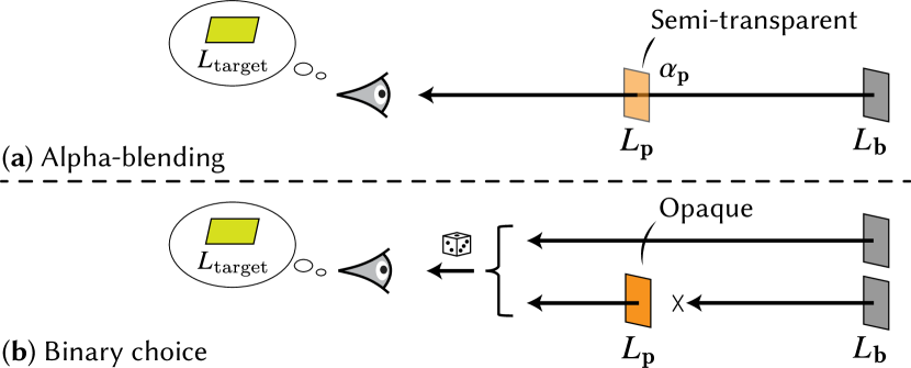
Figure 3. Non-local perturbations. We consider a single candidate surface patch (with color $L_{\mathbf{p}}$) along the ray as a perturbation of a background surface (with color $L_{\mathbf{b}}$). (a) Blending colors violates the surface assumption and leads to volumetric results. (b) We instead treat the perturbation as a random binary choice and optimize the associated discrete probability. The final reconstruction is non-random and will never blend the contribution of multiple surfaces.

Multiple candidates

We now extend the loss formulation to consider multiple candidates. This is advantageous because it will allow our method to simultaneously evaluate the effect of several perturbations, which in turn accelerates convergence.

The key property of the single-candidate loss formulation is that it isolates the candidate from the background surface (i.e., observing one or the other). The generalization to multiple candidates preserves this property by treating each candidate as an independent subproblem (Figure 4), minimizing the sum of respective losses:

(3) $$\mathcal{L}_{\mathrm{ray}}(\mathbf{r})=\sum_{i=1}^{m}\mathcal{L}(\mathbf{p}_{i}),$$

where $\mathcal{L}(\mathbf{p}_{i})$ (following Equation 2) represents the loss of the $i$-th of $m$ candidates sampled along the ray $\mathbf{r}$.

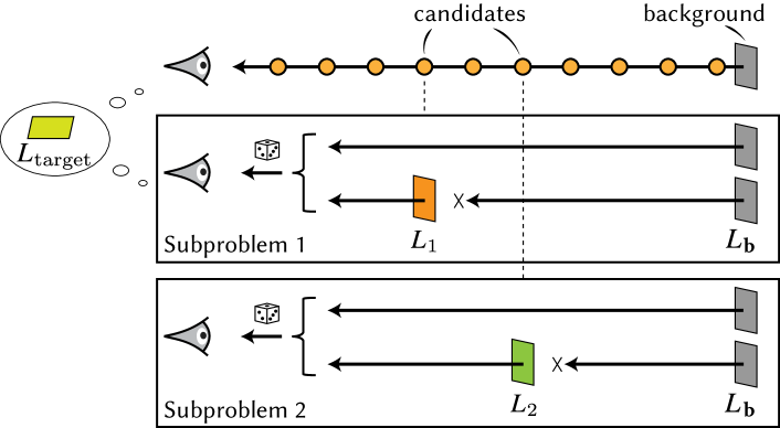
Figure 4. Surface candidates as independent subproblems. With multiple candidates along a ray, each perturbation is treated as an independent subproblem, resulting in local losses distributed spatially over the scene.

Spatio-directional loss

Reconstruction tasks evaluate the loss (3) along a large set of rays $\mathbf{r}_{k}\ (k=1,\ldots,n)$, where $n$ denotes the total number of pixels across all reference images. This further expands the set of independently considered candidate surfaces and leads to the combined loss

(4) $$\mathcal{L}_{\mathrm{total}}=\sum_{k=1}^{n}\mathcal{L}_{\text{ray}}(\mathbf{r}_{k}).$$

Whereas conventional surface optimization only propagates gradients to the surface itself, the use of $\alpha_{\mathbf{p}}$ and $L_{\mathbf{p}}$ in Equation (2) covers the entirety of the observed 3D space. For positions viewed from multiple directions, the loss generally also varies with respect to direction:

In other words: by moving the evaluation of $\ell$ from image space into the scene, we have created a spatio-directional radiance field loss.

3.3. Stochastic background surface

To complete our derivation of the loss function, what remains is the definition of the background surface. Rather than a deterministic surface (e.g., a level set of the occupancy field), we draw the background from a per-ray distribution $f_{\mathbf{b}}$. This enables occasional “visibility” through high-occupancy regions, allowing occluded objects to be considered as the background (Figure 5). Crucially, we thereby support complex topological changes in our optimization without having to explicitly account for them [Mehta et al., 2023]; see Appendix C for additional details.

The design of the distribution $f_{\mathbf{b}}$ is flexible. One straightforward approach is to prioritize sampling in high-occupancy regions, as these areas are more likely to correspond to surfaces. During ray traversal, we stochastically decide whether to use a position as the background surface based on its occupancy value. This sequential decision process reflects the concept of free-flight distance [Novák et al., 2018], forming the free-flight background distribution.

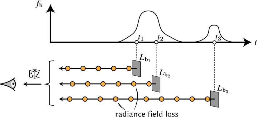
Figure 5. Stochastic background. Selecting the background surface at random from a distribution $f_{\mathbf{b}}$ enables visibility through high-occupancy regions. Each sampled background surface defines a new perturbation problem solvable with the radiance field loss. Taking an expectation of this process leads to a simple deterministic expression that we implement in practice.

We can formulate the expectation of sampling the background surface from such a free-flight distribution analytically and derive a corresponding aggregated local loss analogous to classical volumetric light transport:

(5) $$\mathcal{L}(\mathbf{p}_{i}) =\left(\prod_{j=1}^{i-1}(1-\alpha_{\mathbf{p}_{j}})\right)\alpha_{\mathbf{p}_{i}}\ell(L_{\mathbf{p}_{i}})\,,$$

which, when plugged into Equation (4), yields the radiance field loss (Figure 2). See Appendix A for the complete derivation.

Implementation

An implementation of our loss function can be arranged to resemble the color blending structure of standard volume reconstruction methods like NeRF [Mildenhall et al., 2020]. As such, it is exceedingly simple to implement in existing codebases, as illustrated in the following comparison of pseudocode.

This resemblance also suggests that the optimization landscape of our method is similar to that of NeRF, inheriting its robustness. However, while NeRF’s loss supervises all samples along the ray to collectively match the target color, our loss aims for each sample to match the target color independently or become transparent when the background is a better match. This distinction fundamentally defines our approach as a surface reconstruction algorithm.

3.4. Volume relaxation

We also propose a heuristic-based generalization of our method. It is orthogonal to the above algorithm and optional during training.

While a surface representation offers many advantages, the opaque surface assumption has inherent limitations in certain scenarios. For example, sub-pixel structures are challenging to model with geometry, and a single surface may fail to accurately represent the appearance of directional-varying materials. In these regions, a volumetric representation is more suitable.

Our goal is to relax our method to reconstruct most of the scene as surfaces (regions where low loss can be reached) and use volumetric representations only in the remaining challenging regions. To this end, we first train with our algorithm for $20$k iterations to obtain an initial surface representation. We then identify challenging regions by evaluating where local losses remain high. In subsequent training steps, we relax the surface assumption, allowing volumetric alpha blending in these regions.

After training, rather than extracting a surface, we render the scene volumetrically, with surface regions treated as fully opaque “volumes”. Comparing to a volume scene optimized with NeRF, our method still benefits from the compact representation of surface regions. When accumulating colors along a ray, very few samples are required to saturate the transmittance, leading to faster inference and reduced computational resources during training.

Where not explicitly stated, all results in this paper (marked as “ours”) are trained without volume relaxation.

4. Results

4.1. Novel view synthesis

Visual quality

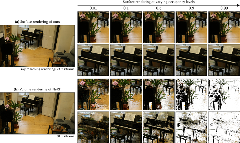
Figure 9. Nature of the reconstructed occupancy. Surface rendering at varying level sets of a scene reconstructed by our method and NeRF, both implemented in Instant NGP using the same hyperparameters. (a) For our method, the surface rendering shows minimal changes across different level set thresholds, indicating that the occupancy field has converged to a near-Heaviside step function on the surface, allowing for extraction of a surface-based representation. (b) NeRF reconstructs the scene volumetrically, and any surface extracted using a level set is a poor approximation of the true color.

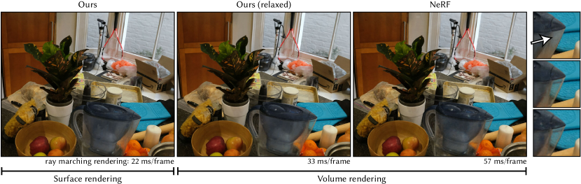
Figure 10. Volumetric relaxation. We compare reconstructions of our method without and with volume relaxation to NeRF, all implemented in Instant NGP using the same hyperparameters. While our method achieves comparable visual quality using a surface-based representation, we highlight a region (white arrow) where it fails to model a semi-transparent object due to the opaque surface assumption. The relaxed variant of our algorithm can recover by adopting volume rendering in such regions. Rendering the reconstructions using the same ray marching implementation leads to significant performance differences: our surface-only reconstruction is $2.6\times$ faster than NeRF. The relaxed variant benefits from the surface representation in most regions, and is $1.7\times$ faster.

Despite the inherently fewer degrees of freedom of surfaces, Figure 9 shows that our method achieves results that are qualitatively comparable to NeRF. We also visualize the surface renderings at occupancy level sets $\{0.01,0.1,0.5,0.9,0.99\}$. Renderings of the scene optimized by our algorithm barely change, indicating a near-Heaviside step function in the occupancy field. In contrast, the inherently volumetric nature of NeRF does not produce meaningful visualizations for these level sets. Figure 10 highlights the reconstruction of another scene where our method with volume relaxation addresses challenges in modeling a semi-transparent object.

Table 1 shows that our method achieves a PSNR only slightly lower than NeRF when trained on the MipNeRF360 dataset with the same hyperparameters, despite employing a surface-based representation. A PSNR gap is expected, as volume representations offer inherently more degrees of freedom that can be repurposed to handle reflections and fine details. This gap is larger in outdoor scenes, in which the far-field is especially hard to model with surfaces.

When training the relaxed variant that switches to volumetric rendering in hard regions in Instant NGP, the visual quality slightly surpasses the NeRF baseline (we measured indoor and outdoor mean PSNRs of $22.62$ dB and $29.41$ dB, respectively). This is because our method promotes surface-like, sparse distributions, leading to more empty space that the underlying rendering algorithm can skip. Consequently, at equal batch size, Instant NGP automatically spawns more rays when using our method, thereby covering more reference pixels per batch, in turn leading to a better reconstruction. When the ray count is restricted to match NeRF, the relaxed variant delivers PSNR results that are approximately equal.

Rendering performance

Our implementation builds on the Instant NGP codebase, which ray-marches fields ($\alpha_{\mathbf{p}},L_{\mathbf{p}}$) represented using an interpolated hash grid lookup combined with a lightweight MLP. We repurpose this ray-marching code for surface rendering by returning the color of the first sample with an occupancy value exceeding $0.5$. This straightforward modification results in an $2.4\times$ average speedup in frames per second (FPS) across MipNeRF360 scenes compared to the baseline. An average speedup of $2.0\times$ is achieved for the relaxed version of our method, as most of the scene remains surface-like.

An additional $2\times$ speedup can be achieved by replacing ray-marching with rasterization of a meshed isosurface. In this case, the color network is only used for mesh shading, maintaining the same visual quality as before. Various strategies exist to further boost rendering performance, e.g., by storing precomputed hash grid lookups alongside mesh vertices [Chen et al., 2023], or by projecting the directional MLP dependence into spherical harmonics [Reiser et al., 2024].

Table 1. PSNR comparison. We integrate our loss into Instant NGP and ZipNeRF and train on the MipNeRF360 dataset using default hyperparams.

	Instant NGP codebase		ZipNeRF codebase
	Ours	NeRF	Ours	NeRF
Indoor mean	22.41 dB	22.47 dB	24.06 dB	25.24 dB
Outdoor mean	29.02 dB	29.19 dB	29.73 dB	31.45 dB

4.2. Geometry reconstruction

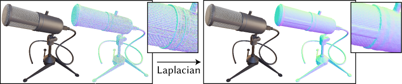
Figure 6. Regularization. For simple scenes with enough observations, the reconstructed surface closely matches the ground truth geometry without requiring additional constraints. Adding Laplacian refinement helps smooth out unnecessary small kinks, resulting in a more accurate final geometry.

Our method is also applicable to geometry reconstruction tasks, in which achieving high-quality meshes matching the ground truth geometry is of interest. For simple multi-view input (Figure 6), our method produces highly detailed geometry with the speed of Instant NGP (seconds). A mesh can be extracted at any point during the optimization (Figure 7). However, complex real-world reconstruction tasks are often under-constrained. For example, a reflective object seen only from a narrow cone of directions does not provide sufficient information for accurate shape recovery. Even with a larger set of viewpoints, it can be challenging to disambiguate whether surface detail is due to local color variation or small-scale geometry. As a consequence, the reconstructed geometry often exhibits undesirable bump-like artifacts representing such misattributed detail. While our algorithm still excels at novel view synthesis under these conditions, the reconstructed geometry can significantly deviate from the ground truth.

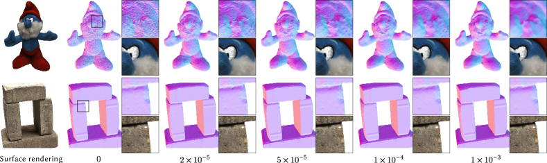
Figure 11. Effect of Laplacian weight on geometry reconstruction. The above results demonstrate the trade-off between geometric detail and surface smoothness. For simple scenes lacking intricate features (bottom row), the reconstruction is insensitive to this hyperparameter.

To mitigate this issue, we incorporate an exponentially decaying Laplacian regularizer during training. This regularizer initially enforces flat surfaces and progressively provides more degrees of freedom as its influence decays. Figure 11 examines the influence of the final Laplacian weight on reconstruction quality. Figure 12 showcases geometry reconstructions of scenes from the DTU [Jensen et al., 2014] and BlendedMVS [Yao et al., 2020] datasets, all made with a consistent Laplacian weight of $2\times 10^{-5}$.

Laplacian regularization is only the first step in a long sequence of potential improvements that can further boost geometric reconstruction quality. These include multi-view consistency losses [Fu et al., 2022; Chen et al., 2024a] to reduce ambiguities in regions with limited observations, or the TSDF algorithm [Izadi et al., 2011] that helps extract smooth meshes while removing unnecessary geometry. We do not intend to compete on geometric reconstruction metrics and have not incorporated such extensions, which would detract from the simplicity of the presented idea.

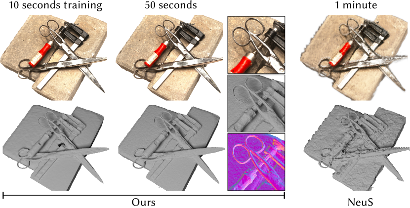
Figure 7. Straightforward extraction. Since our algorithm does not use an intermediate volume representation, efficient surface extraction is possible at any point. At equal time, a fast NeuS baseline [Wang et al., 2023] still models the scene as a fuzzy volume, and a surface cannot be confidently extracted.

5. Discussion

5.1. Choice of background distribution

In Section 3.3, we used the free-flight background distribution to derive a loss form dual to the NeRF loss. This choice is somewhat arbitrary, and other distributions could be used with different trade-offs. In Appendix B, we discuss how alternative designs can enable new optimization strategies that are not possible in image-space methods, with one such example provided.

5.2. Relation to many-worlds inverse rendering

Our method builds on the core idea of Zhang et al. [2024] (we refer to their method as PBR-MW), namely that surface distributions can be optimized more directly without involving exponential volumes. We reconstruct purely emissive objects, while PBR-MW handles differentiable shadowing and interreflection to reconstruct reflecting objects in scenes with global illumination. Viewed superficially, our method could be mistaken for a stripped down version of PBR-MW.

Our contribution lies in leveraging this simplicity to develop a specialized method. We identify and implement optimizations unique to emissive surfaces to fully realize the potential of the many-worlds idea.

In emissive surface rendering, image formation is a direct 1:1 mapping between a ray and the nearest intersected emissive surface, while PBR-MW requires a complex nested integration over materials, lighting, and geometry. Our approach to project training images into the scene to establish a radiance field loss depends on this 1:1 mapping and does not efficiently translate to the nested integral structure of a global illumination renderer.

Another important contribution is the introduction of a stochastic background distribution, which enables topological changes and substantially improves reconstruction quality. We show how to cheaply evaluate this strategy in expectation, which is needed to maintain algorithmic parity with NeRF. The associated derivations and simplifications (Appendix A) are specific to emissive surfaces and do not transfer to PBR-MW.

5.3. Limitations and future work

Moving the evaluation of the color loss $\ell$ from image space into the radiance field makes our method incompatible with loss functions that depend on image-space neighborhoods (e.g., style losses).

As shown in Figure 8, our lightweight Laplacian regularization fails when there are insufficient observations to constrain the geometry. Using alternative regularization techniques from state-of-the-art geometry reconstruction methods could help mitigate this issue. Our method also struggles to accurately capture the appearance of conductive materials, which could be addressed by incorporating solutions from prior work [Verbin et al., 2021].

An interesting extension of our work could involve implementing a particle-based storage approach, such as Gaussian splatting [Niemeyer et al., 2020]. However, 3D Gaussians are inherently semi-transparent, which conflicts with our assumption of opacity. Future work could explore the use of opaque primitives, such as 2D disks, to replace semi-transparent particles.

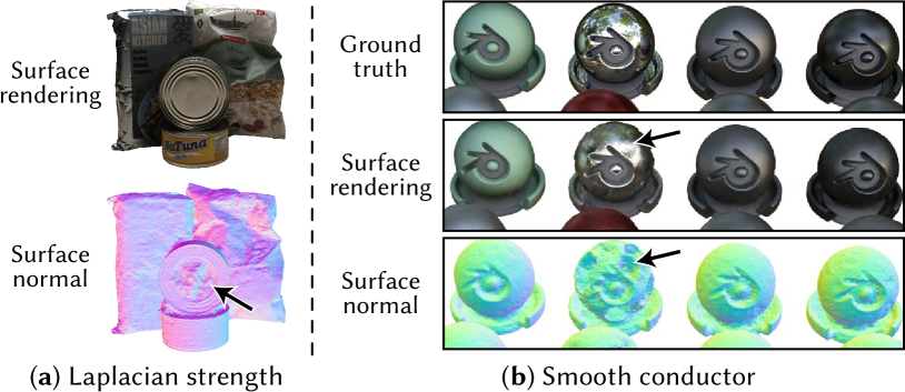
Figure 8. Limitations. (a) Our Laplacian smoothing strategy fails to reconstruct the flat can surface due to its view-dependent appearance. A larger Laplacian weight can help, but this also suppresses geometric detail seen in Figure 12. (b) High-frequency color variation is more challenging to accurately represent on a surface compared to a volumetric representation.

6. Conclusion

The ”many worlds” paradigm—i.e., optimizing a distribution over non-interacting primitives—is relatively new in the field of differentiable rendering. In this paper, we apply it to emissive surface reconstruction, which yields a fast and simple alternative to prior works. Particularly notable is that the derivation began with an evolving surface, yet resulted in remarkably similar equations to volumetric scene reconstructions: ones where losses rather than colors are integrated along rays.

As reconstruction tasks increase in difficulty, a key challenge lies in deciding whether a region of space is best represented by a surface or a volume. While the relaxed variant of our method offers an effective heuristic, it also underscores the need for a principled answer to this important question.

Much engineering has gone into the design of optimized algorithms, regularizers, and heuristics for NeRF-based 3D reconstruction. Our hope is that a large portion of this effort will translate to the radiance field loss and yield state of the art results in the future.

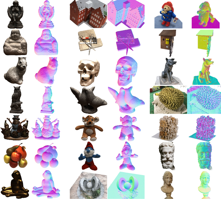
Figure 12. Reconstruction showcase. Surface rendering and normals of various scenes from the DTU and BlendedMVS datasets, reconstructed with our algorithm and a decaying Laplacian. All results were generated with the same hyperparameters and a training time of $\sim 1$ minute per scene.

Appendix A Derivation of our loss in NeRF form

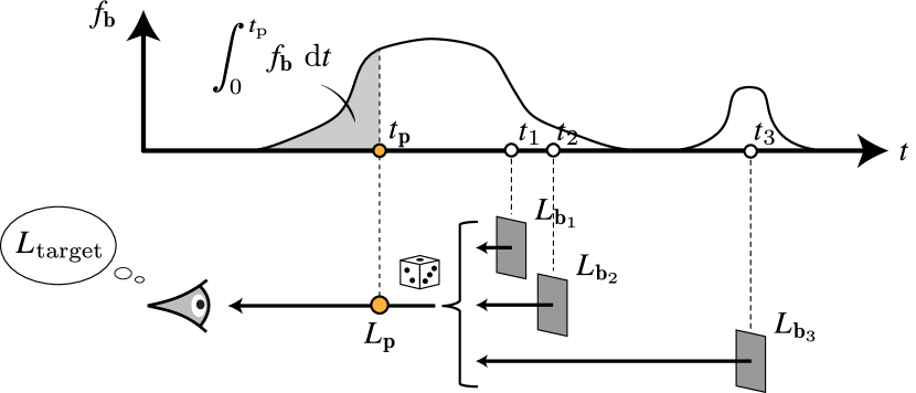
Figure 13. We derive an analytic loss expectation over all possible background surfaces for a specific candidate position at $t_{\mathbf{p}}$.

Following the introduction of the radiance field loss and the stochastic background, a naive implementation of our method would first sample a surface $\mathcal{M}_{\text{b}}$ from a distribution as the perturbation background, and for each sampled $\mathcal{M}_{\text{b}}$, we need to sample multiple candidates to solve the non-local perturbation problem. Naively applying this strategy would result in a quadratic time complexity. In the following, we derive an expectation of losses over all potential background surfaces (Figure 13) for a specific candidate.

Let $f_{\mathbf{b}}$ be the probability distribution of the background surface along a ray, where $\int_{0}^{t_{\mathrm{max}}}f_{\mathbf{b}}(t)\,\mathrm{d}t=1$. Without loss of generality, we focus on one candidate position $\mathbf{p}$ at distance $t_{\mathbf{p}}$ along the ray. To avoid clutter, we denote the color error metric $\ell(L,~L_{\mathrm{target}})$ as $\ell(L)$. The expectation of all losses in the form of Equation 2, local at $\mathbf{p}$, is given by:

$$\mathbb{E}[\mathcal{L}(\mathbf{p})] =\int_{t_{\mathbf{p}}}^{t_{\mathrm{max}}}\mathcal{L}(\mathbf{p})\,f_{\mathbf{b}}(t)\,\,\mathrm{d}t$$

$$=\int_{t_{\mathbf{p}}}^{t_{\mathrm{max}}}\left(\alpha_{\mathbf{p}}\,\ell(L_{\mathbf{p}})+(1-\alpha_{\mathbf{p}})\,\ell(L_{t})\right)\,f_{\mathbf{b}}(t)\,\mathrm{d}t$$

$$=\left(1-\int_{0}^{t_{\mathbf{p}}}f_{\mathbf{b}}(t)\,\mathrm{d}t\right)\alpha_{\mathbf{p}}\,\ell(L_{\mathbf{p}})~+$$

(6) $$\qquad\qquad\qquad\qquad(1-\alpha_{\mathbf{p}})\int_{t_{\mathbf{p}}}^{t_{\mathrm{max}}}\ell(L_{t})\,f_{\mathbf{b}}(t)\,\mathrm{d}t.$$

Let $\mathbb{E}_{t>t_{\mathbf{p}}}[\ell(L_{t})]$ be the expectation of error metrics for $t>t_{\mathbf{p}}$. We can rewrite the result as:

(7) $$\mathbb{E}[\mathcal{L}(\mathbf{p})] =\Big{(}\underbrace{1-\int_{0}^{t_{\mathbf{p}}}f_{\mathbf{b}}(t)\,\mathrm{d}t}_{\mathrm{weight}}\Big{)}\Big{(}\alpha_{\mathbf{p}}\,\underbrace{\ell(L_{\mathbf{p}})}_{\mathrm{candidate}}+~(1-\alpha_{\mathbf{p}})\underbrace{\mathbb{E}_{t>t_{\mathbf{p}}}[\ell(L_{t})]}_{\mathrm{background}}\Big{)}.$$

Equation 7 reflects an aggregated form of non-local perturbation, where the background color is treated as an expectation over all possible background surfaces rather than a fixed value. The weight term captures the probability of selecting a background surface located behind the perturbation position. The expectation computation should not change the loss landscape, so the weight term should not be differentiated during optimization.

In the following, we analyze the discrete case of the loss expectation along a ray with $m$ sampled points, assuming the free-flight background distribution $f_{\mathbf{b}}$. For simplicity, we denote the occupancy and color at position $\mathbf{p}_{i}$ as $\alpha_{i}$ and $L_{i}$, respectively. The summation of all losses is given by:

(8) $$\mathcal{L}_{\mathrm{ray}} =\sum_{i=1}^{m}\hat{\mathbb{E}}[\mathcal{L}(\mathbf{p}_{i})]$$

$$=\sum_{i=1}^{m}\Bigg{[}\Big{(}\underbrace{\prod_{k=1}^{i-1}(1-\alpha_{k})}_{\mathrm{weight}}\Big{)}\Big{(}\alpha_{i}\,\underbrace{\ell(L_{i})}_{\mathrm{candidate}}+(1-\alpha_{i})\,\underbrace{\hat{\mathbb{E}}_{t>t_{i}}[\ell(L_{t})]}_{\mathrm{background}}\Big{)}\Bigg{]},$$

where

(9) $$\hat{\mathbb{E}}_{t>t_{i}}[\ell(L_{t})]=\sum_{j=i+1}^{m}\left(\prod_{t=i+1}^{j-1}(1-\alpha_{t})\right)\,\alpha_{j}\,\ell(L_{j}).$$

Not all variables in this loss function are meant to be differentiated. Specifically, the weight term and the background are treated as constants in the optimization process and are excluded from differentiation (i.e., detached). To indicate which terms should be differentiated, we underline them in the derivation as $\uuline{{\color[rgb]{0,0,0}(\cdot)}}$.

Below, we reformulate the loss function into a structure similar to the NeRF loss function. We take some notational liberty of using $\operatorname*{argmin}$ to transform the equation in such a way that its derivatives and the location of minima are preserved, but the loss value may differ by a constant value.

Equation 8 then becomes equivalent to minimizing:

$$\operatorname*{argmin}\sum_{i=1}^{m}\left[\left(\prod_{k=1}^{i-1}{(1-\alpha_{k})}\,\right)\left(\uuline{{\color[rgb]{0,0,0}\alpha_{i}}}\,\ell(\uuline{{\color[rgb]{0,0,0}L_{i}}})+(1-\uuline{{\color[rgb]{0,0,0}\alpha_{i}}})\,\hat{\mathbb{E}}_{t>t_{i}}[\ell(L_{t})]\right)\right]$$

$$= \operatorname*{argmin}\underbrace{\sum_{i=1}^{m}\left(\prod_{k=1}^{i-1}(1-\alpha_{k})\right)\alpha_{i}\,\ell(\uuline{{\color[rgb]{0,0,0}L_{i}}})\,}_{\mathrm{(a)}}+\underbrace{\sum_{i=1}^{m}\left(\prod_{k=1}^{i-1}(1-\alpha_{k})\right)\uuline{{\color[rgb]{0,0,0}\alpha_{i}}}\,\ell(L_{i})\,}_{\mathrm{(b)}}$$

(10) $$\quad\quad+\underbrace{\sum_{i=1}^{m}\left(\prod_{k=1}^{i-1}{(1-\alpha_{k})}\right)\left((1-\uuline{{\color[rgb]{0,0,0}\alpha_{i}}})\,\hat{\mathbb{E}}_{t>t_{i}}[\ell(L_{t})]\right),}_{\mathrm{(c)}}$$

where the terms $\mathrm{(a)}$ and $\mathrm{(b)}$ arise from an application of the product rule. Reordering the double summation in term $\mathrm{(c)}$ yields:

$$\mathrm{(c)} \overset{\eqref{eq:background_exp}}{=}\sum_{i=1}^{m}\sum_{j=i+1}^{m}\left(\prod_{k=1}^{i-1}{(1-\alpha_{k})}\,\right)\left((1-\uuline{{\color[rgb]{0,0,0}\alpha_{i}}})\,\left(\prod_{t=i+1}^{j-1}{(1-\alpha_{t})}\,\right){\alpha_{j}\,\ell(L_{j})}\right)$$

(11) $$=\sum_{j=1}^{m}\,\,\sum_{i=1}^{j-1}\,\,\,\left(\prod_{k=1}^{i-1}{(1-\alpha_{k})}\,\right)\left((1-\uuline{{\color[rgb]{0,0,0}\alpha_{i}}})\,\left(\prod_{t=i+1}^{j-1}{(1-\alpha_{t})}\,\right){\alpha_{j}\,\ell(L_{j})}\right).$$

We rename the indices $i\leftrightarrow j$ and subsequently simplify the expression to:

$$(\ref{eq:loss_c1}) =\sum_{i=1}^{m}\sum_{j=1}^{i-1}\left(\prod_{k=1}^{j-1}{(1-\alpha_{k})}\,\right)\left((1-\uuline{{\color[rgb]{0,0,0}\alpha_{j}}})\,\left(\prod_{t=j+1}^{i-1}{(1-\alpha_{t})}\,\right){\alpha_{i}\,\ell(L_{i})}\right)$$

(12) $$=\sum_{i=1}^{m}\sum_{j=1}^{i-1}\prod_{\begin{subarray}{c}k=1\\ k\neq j\end{subarray}}^{i-1}{(1-\alpha_{k})}\,(1-\uuline{{\color[rgb]{0,0,0}\alpha_{j}}})\,{\alpha_{i}\,\ell(L_{i})}.$$

Combining the term $\mathrm{(c)}$ in the form of Appendix A with the term $\mathrm{(b)}$, we obtain:

$$\mathrm{(b)}\!+\!\mathrm{(c)} =\sum_{i=1}^{m}\left(\prod_{k=1}^{i-1}{(1-\alpha_{k})}\,\uuline{{\color[rgb]{0,0,0}\alpha_{i}}}+\sum_{j=1}^{i-1}\prod_{\begin{subarray}{c}k=1\\ k\neq j\end{subarray}}^{i-1}{(1-\alpha_{k})}\,(1-\uuline{{\color[rgb]{0,0,0}\alpha_{j}}})\,{\alpha_{i}}\right)\,\ell(L_{i})$$

(13) $$=\sum_{i=1}^{m}\left(\prod_{k=1}^{i-1}(1-\uuline{{\color[rgb]{0,0,0}\alpha_{k}}})\,\uuline{{\color[rgb]{0,0,0}\alpha_{i}}}\,{\ell(L_{i})}\,\right)+c_{1},$$

where $c_{1}$ is a constant value. Finally, we can insert this result back in Appendix A to obtain a loss where all variables can be differentiated:

$$\operatorname*{argmin}~\mathrm{(a)}\!+\!\mathrm{(b)}\!+\!\mathrm{(c)}$$

$$\overset{\eqref{eq:loss_c3}}{=} \operatorname*{argmin}\sum_{i=1}^{m}\left(\prod_{k=1}^{i-1}(1-\uuline{{\color[rgb]{0,0,0}\alpha_{k}}})\,\uuline{{\color[rgb]{0,0,0}\alpha_{i}}}\,{\ell(L_{i})}\,+\prod_{k=1}^{i-1}{(1-\alpha_{k})\,\alpha_{i}}\,\ell(\uuline{{\color[rgb]{0,0,0}L_{i}}})\,\right)$$

(14) $$= \operatorname*{argmin}\sum_{i=1}^{m}\left(\prod_{k=1}^{i-1}(1-\uuline{{\color[rgb]{0,0,0}\alpha_{k}}})\,\uuline{{\color[rgb]{0,0,0}\alpha_{i}}}\,\ell(\uuline{{\color[rgb]{0,0,0}L_{i}}})\right).$$

This final result is equivalent to the one shown in Figure 2. It is now also apparent that we do not need to produce extra samples to evaluate $\mathbb{E}_{t>t_{\mathbf{p}}}[\ell(L_{t})]$, thereby reducing the algorithm’s time complexity to a linear one.

Appendix B Design space of the background distribution

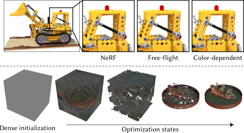
Figure 14. Benefits of the color-dependent background distribution. (Top) After $2000$ iterations, the color-dependent variant explores further along the ray and clears over aggressively optimized regions faster. (Bottom) In a contrived experiment where the scene is densely initialized, the optimizer first attempts to bake the images onto the cube. The color-dependent variant can penetrate high-occupancy regions, while others get stuck. All experiments are conducted with the same hyperparameters in the Instant NGP [Müller et al., 2022] codebase.

Section 3.3 proposes the stochastic background surface. Designing the background surface distribution $f_{\mathbf{b}}$ (Figure 13) involves a tradeoff between exploitation and exploration, offering a wide design space.

On one hand, choosing a background surface close to the model’s current best guess (i.e., in high occupancy regions) ensures that only perturbations with an improvement will be accepted. An example is the deterministic strategy to always use the $0.5$ level set. It aggressively selects the first potential surface with more than $50\%$ confidence along the ray as the background, ignoring any further possibilities.

On the other hand, exploring more possibilities enhances the algorithm’s robustness in scenes with complex occlusions. The free-flight background distribution is a softer version of the deterministic strategy. Instead of using a threshold to binarize the occupancy field, it stochastically decides whether to use a surface as the perturbation background during ray traversal.

Many other designs are possible. One unique to our method is the color-dependent background distribution. Unlike the free-flight distribution, which relies only on the occupancy value, this approach also considers how well each potential surface aligns with the target color, measured by $\ell(L_{\mathbf{p}},\,L_{\mathrm{target}})$. The additional information enables us to discard high-occupancy surfaces that poorly match the target color, which may result from overly aggressive optimization. Specifically, we compute an effective occupancy $\alpha^{\prime}$, as a modification of the original occupancy $\alpha$:

$$\alpha^{\prime}=\frac{\alpha}{1+c\,\ell(L_{\mathbf{p}},L_{\mathrm{target}})}.$$

When the color matches well, the transformation is neutral, but for misaligned colors, it reduces the effective occupancy, lowering the likelihood of selecting such surfaces as a background. In our experiments, we used $c=16$. As shown in Figure 14, this color-dependent distribution can be more efficient when penetrating incorrect surfaces.

This expanded design space is particularly compelling. Traditional reconstruction methods mostly optimize in image space, interacting with the 3D scene only through a rendering algorithm (surface-based or volume-based). As a result, the design space in image space is quite limited, with little to do beyond computing a loss.

In contrast, our method operates directly in the scene space. Background distributions can be tailored to focus on regions of interest. This flexibility enables the development of new optimization strategies that are unattainable in image-space methods. The color-dependent background distribution is an example to actively guide the optimization to skip regions that are believed to be wrong regardless of the occupancy value.

In this paper, we focus on the free-flight distribution to highlight the dual-loss relationship with NeRF, leaving the exploration of other distributions for future work. Only the result in Figure 14 uses the color-dependent distribution.

Appendix C Additional experiments and results

Interior topology changes

Methods based on local surface evolution struggle with interior topological changes, like transforming a sphere into a torus. Indeed, they primarily rely on deforming visibility silhouettes to change the overall shape, but these silhouettes often do not exist in regions away from the outer contour.

Correctly handling such topological changes requires making a significant modification, such as cutting a cone through the entire object to expose the occluded background. This type of change is beyond the reach of common derivative-based methods, which can only account for infinitesimal perturbations.

Mehta et al. [2023] propose a cone-shaped perturbation strategy to test whether exposing the background improves the match to the target color in the application of physically based rendering. This approach significantly improves convergence in scenes that require hole penetration, compared to conventional surface evolution methods.

However, this strategy can also affect scenes where the topology is already correct. In such cases, only local refinement is needed, and the cone perturbation may bias the derivative in the wrong direction. Additionally, the cone perturbation strategy can only penetrate a single obstacle, limiting its ability to handle complex real-world scenes that require penetration through multiple layers of geometry (Figure 15). Our stochastic background strategy addresses these challenges by considering additional background possibilities, enabling more robust optimization for complex scenes.

Rendering

Once the occupancy field trained with our algorithm has converged, it should have value $0$ in empty space and $1$ on the surface. Since our field storage is continuous in practice, we aim for a near Heaviside step function on the surface. In Figure 20, we show an additional level set rendering result for an outdoor scene to demonstrate that our method can achieve this, with any level set being usable. In this paper we use $0.5$ as the threshold.

We propose two methods for rendering the level set. The first method involves ray marching with a small step size. In this approach, we immediately return the color of the first sample point that hits the surface (when occupancy exceeds $0.5$), without any weighting or color blending. The second method involves extracting a triangle mesh using marching cubes or TSDF fusion, then rasterizing the mesh to obtain the hit point location and querying the color network for the final color.

Both methods produce nearly identical visual results, as shown in Figure 16.

Codebase

Our work primarily focuses on the theoretical development of a surface-based scene reconstruction algorithm, while the specifics of the model implementation are largely independent of our core algorithm. For example, the Instant NGP codebase is optimized for speed and designed for object-centric scenes, resulting in suboptimal details in the far field background (Figure 17). Our results inherit these advantages and limitations.

Decaying Laplacian

For simple scenes with sufficient observations, Laplacian smoothing as a post-processing step can effectively refine surface geometry. However, this approach has limitations in more challenging scenarios. As shown in Figure 18, we analyze a highly underconstrained scene with shiny surfaces that exhibit rapid color changes with viewing angle, captured only from the front. Here, training without Laplacian smoothing achieves good novel view synthesis but results in geometry errors, particularly at the can’s bottom.

Applying a Laplacian as a post-processing step requires numerous iterations to address these issues and may degrade geometry in other regions. In contrast, training our algorithm with an exponentially decaying Laplacian is more efficient. Consequently, the results in Figure 12 are obtained by training our algorithm with an exponentially decaying Laplacian.

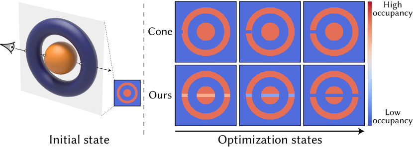
Figure 15. Left: We test interior topological changes in a scene where orange better aligns with the target background color than indigo. Right: We show optimization states by visualizing a 2D slice of the occupancy field. The cone perturbation strategy [Mehta et al., 2023] gets stuck after penetrating the torus once, as it can only see through a single obstacle.

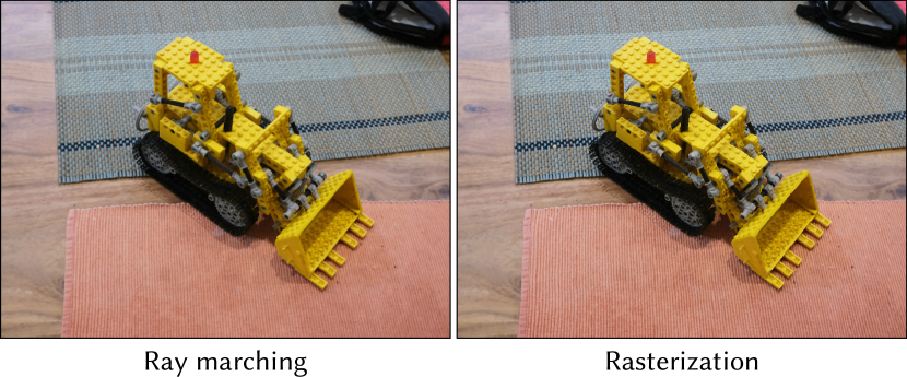
Figure 16. Visual comparison of the same surface scene trained with our algorithm using two rendering methods: ray marching (left) and mesh rasterization (right). Both methods give nearly identical results.

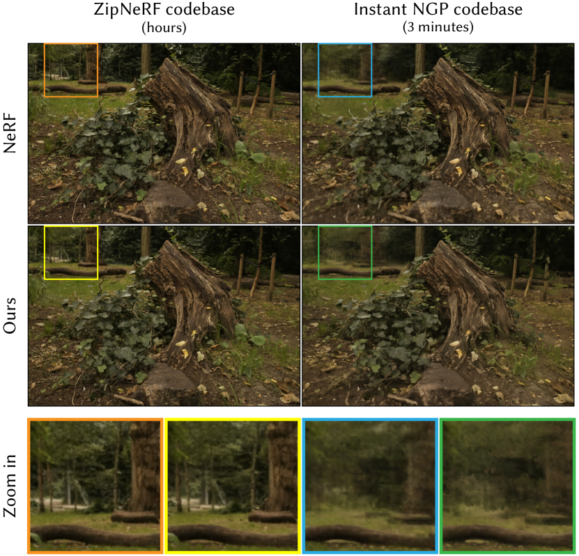
Figure 17. Qualitative comparison of NeRF and our method in two codebases.

Training time

Figure 19 shows the loss convergence plot in the Instant NGP codebase, demonstrating that our method converges at a rate comparable to NeRF despite its surface reconstruction nature.

Like NeRF, our method computes the loss in linear time only using per-sample occupancy and color values along a ray. Theoretically, this ensures it is at least as fast as NeRF. However, the observed increase in training time arises from INGP’s training strategy, which targets a fixed sample size per iteration (we use the default value $2^{18}$) by spawning as many rays as needed. Since our method reconstructs surfaces, it typically requires fewer samples along rays in near-converged regions, allowing more rays to be processed within the same sample budget. In practice, the increase in ray count causes INGP to become slower.

This slowdown is a consequence of INGP’s implementation rather than a limitation of our method. In fact, our method’s efficiency in using fewer resources per ray is advantageous. This also explains why our relaxed variant achieves a higher PSNR than NeRF: it utilizes the same sample budget to visit more reference pixels per iteration.

Miscellaneous

Figure 20 shows additional level set rendering results for an outdoor scene. Table 2 and Table 3 show the complete PSNR and SSIM results in the Instant NGP codebase. Table 4 shows the complete PSNR results in the ZipNeRF codebase.

Appendix D Volume relaxation

This section details a heuristic-based volume relaxation of our method. While we do not claim this to be the only way to relax our method, it provides a straightforward and effective way to retain the surface-like properties of the scene while enabling volumetric blending in regions where the surface representation is insufficient.

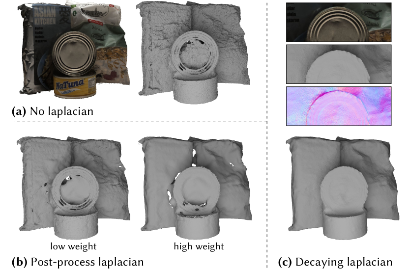
Figure 18. For highly underconstrained scenes with shiny surfaces and limited viewing angles, training our algorithm with an exponentially decaying Laplacian is more effective than applying Laplacian as a post-processing step.

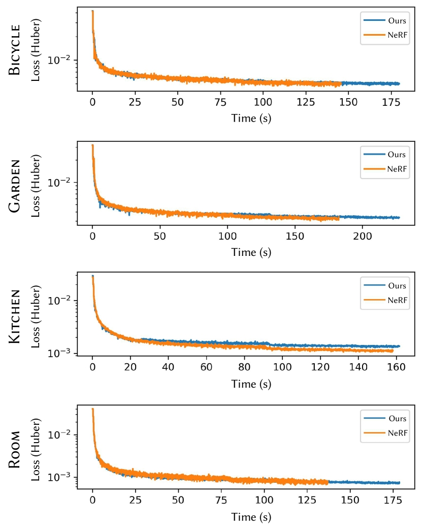
Figure 19. Equal time PSNR curve plot. Our method converges at a rate comparable to NeRF in the Instant NGP codebase. We have a longer tail in the loss curve since our method spawns more rays per iteration than NeRF.

We propose the following loss function as a relaxed volumetric version of our loss in the form of Equation 8. The notation $\uuline{{\color[rgb]{0,0,0}(\cdot)}}$ is consistent with Appendix A, denoting terms that are differentiated during optimization:

(15) $$\mathcal{L}_{\mathrm{ray}}^{\mathrm{vol}}=\sum_{i=1}^{m}\left[\left(\prod_{k=1}^{i-1}(1-\alpha_{k})\right)\,\ell\Big{(}\uuline{{\color[rgb]{0,0,0}\alpha_{i}}}\,\uuline{{\color[rgb]{0,0,0}L_{i}}}+(1-\uuline{{\color[rgb]{0,0,0}\alpha_{i}}})\,\mathbb{E}_{t>t_{i}}[L_{t}],\,L_{\mathrm{goal}}\Big{)}\right],$$

where the error metric $\ell$ now compares against a modified target color $L_{\mathrm{goal}}$:

(16) $$L_{\mathrm{goal}}=\frac{L_{\mathrm{target}}-L_{\mathrm{prev}}}{T_{\mathrm{prev}}}=\frac{L_{\mathrm{target}}-\sum_{j=1}^{i-1}\left(\prod_{k=1}^{j-1}(1-\alpha_{k})\right)\alpha_{j}L_{j}}{\prod_{j=1}^{i-1}(1-\alpha_{j})}.$$

Equation 15 is derived from two key modifications to the radiance field loss (Equation 8):

• We now blend colors instead of error metrics to allow for volumetric blending for the $i$-th sample.

• The $i$-th sample no longer needs to match the target color $L_{\mathrm{target}}$ directly. Instead, its goal adjusts for the color contribution of prior samples $L_{\mathrm{prev}}$ and the transmittance from the camera to the $i$-th sample $T_{\mathrm{prev}}$.

Empirically, this relaxed loss performs well as a volume reconstruction algorithm. However, when used to refine a converged surface scene, this loss often converts the entire scene into a volumetric representation, even in regions where the surface representation is already visually adequate. This happens because a surface representation is essentially a special case of a volume with fewer degrees of freedom, and fitting colors in a volume generally reduces the loss more easily than fitting colors on a surface.

To prevent over-relaxation, we propose a heuristic to detect locations where volume relaxation is unnecessary. Specifically, when the local loss without blending at a specific position is no worse than the local loss with blending:

(17) $$\ell(L_{i},L_{\mathrm{goal}})\leq\ell\left(\alpha_{i}\,L_{i}+(1-\alpha_{i})\,\mathbb{E}_{t>t_{i}}[L_{t}],\,L_{\mathrm{goal}}\right),$$

we use the local loss without blending in Equation 15. This comparison does not introduce any overhead, as all necessary values are already available. Our experimental results show that this heuristic is effective in preserving Heaviside-like occupancy values in most areas while allowing for volumetric blending in challenging regions (Figure 20).

We highlight again that the volume relaxation step is a heuristic and not a fundamental part of our method. All results are obtained without this relaxation in this paper unless explicitly stated.

Appendix E Implementation details

All results were generated and measured on a Linux workstation with an AMD Ryzen 7950X processor and an NVIDIA RTX 4090 graphics card.

Instant NGP codebase

We used the default hyperparameter configuration file (base.json) provided by the authors and retained the original sampling strategy. However, we made two key modifications to the codebase to accommodate our method:

• We reduced the ray marching step size from $1/1024$ to $1/2048$ to achieve a finer surface resolution.

• The maximum buffer size for storing temporary samples was increased from $16\times\mathrm{target~batch~size}$ to $128\times\mathrm{target~batch~size}$ to accommodate the increased number of rays spawned in each iteration.

Since INGP does not natively support automatic differentiation, we manually implemented the derivative propagation of our method into the codebase, similar to how the framework trains NeRF.

For the geometry reconstruction experiments shown in Figure 12, we used a $L_{1}$ loss to improve convergence in dark regions. Models were trained for $10000$ iterations (reduced from the default $35000$), with the Laplacian weight decaying exponentially to $2\times 10^{-5}$. The Laplacian was estimated via finite differences using six neighboring samples with an epsilon of $1/1024$ (approximately 1 mm for a unit cube).

Rendering times were measured without DLSS.

ZipNeRF codebase

We used the default hyperparameter configuration file (360.gin) along with the original adaptive sampling strategy. As ZipNeRF’s adaptive sampling is tailored for volume reconstruction, it may not be optimal for our method. However, we deliberately avoided modifying these components to minimize intrusive changes and focus on proof-of-concept validation.

Warm start

During training, our algorithm can sometimes push occupancy values in certain regions (e.g., peripheral or camera-adjacent areas) too high in early stages, resulting in floaters in the final reconstruction. This occurs because the background is insufficiently explored at the beginning, leading to overly aggressive optimization of temporarily superior candidates. While NeRF encounters similar issues, recovery is particularly challenging in our case since occupancy values of these floaters could approach $1$.

For INGP training, we can mitigate this issue by adjusting the learning rate schedule at the cost of slower convergence. Empirically, we found it also effective to impose a moving upper bound on occupancy values, gradually relaxing this constraint during training. Specifically, at iteration $i$, we bound the occupancy value by $\alpha_{\mathrm{max}}=0.1+0.9\times i/1000$. This constraint is active only during the first $1000$ iterations, corresponding to the first few seconds of training. Additionally, we observed that our relaxed training strategy is less prone to floaters. For novel view synthesis tasks, we trained the relaxed variant for $5000$ iterations as a warm start.

The floater issue also pops up in the ZipNeRF codebase. For simplicity, we adopted a NeRF training warm start during the first 5% of training iterations and did not bound occupancy values.

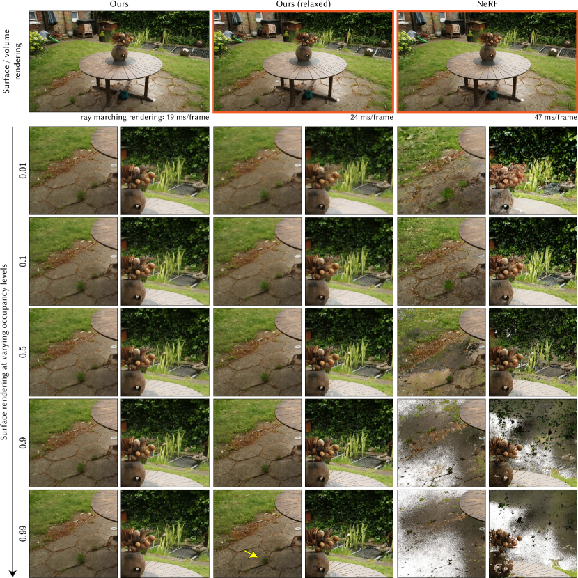
Figure 20. Surface rendering at varying level sets of a scene reconstructed by our method and NeRF, using the same hyperparameters. Only the two images with orange borders are rendered volumetrically. Left: For our method, the surface rendering shows minimal changes across different level set thresholds, indicating that the occupancy field has converged to a near-Heaviside step function on the surface. Middle: The relaxed variant of our algorithm uses volume representation in challenging regions, such as sub-pixel details (yellow arrow). The overall scene remains surface-like, leading to better ray marching performance than NeRF. Right: The NeRF reconstruction is inherently volumetric, thus renderings of level sets do not produce meaningful visualizations.

Table 2. PSNR comparison using the Instant NGP codebase. Ours uses surface rendering, while the relaxed variant and NeRF use volume rendering.

	Bicycle	Bonsai	Counter	Garden	Kitchen	Room	Stump	Flowers	Treehill
Ours	22.53	31.22	26.67	23.81	28.58	29.59	24.16	19.76	21.79
Ours (relaxed)	22.66	31.81	26.95	24.04	29.14	29.75	24.43	19.98	21.97
NeRF	22.66	31.45	26.79	23.97	29.33	29.17	23.96	19.95	21.82

Table 3. SSIM comparison using the Instant NGP codebase.

	Bicycle	Bonsai	Counter	Garden	Kitchen	Room	Stump	Flowers	Treehill
Ours	0.673	0.918	0.872	0.577	0.686	0.866	0.896	0.769	0.692
Ours (relaxed)	0.682	0.927	0.882	0.590	0.695	0.878	0.902	0.784	0.698
NeRF	0.675	0.924	0.877	0.586	0.687	0.877	0.893	0.776	0.692

Table 4. PSNR comparison using the ZipNeRF codebase.

	Bicycle	Bonsai	Counter	Garden	Kitchen	Room	Stump	Flowers	Treehill
Ours	24.10	31.24	26.38	26.14	30.22	31.07	25.96	20.99	23.12
NeRF	25.50	33.20	28.16	27.62	32.01	32.44	27.11	22.11	23.85

References

- [1]
- Chen et al. [2024a] Danpeng Chen, Hai Li, Weicai Ye, Yifan Wang, Weijian Xie, Shangjin Zhai, Nan Wang, Haomin Liu, Hujun Bao, and Guofeng Zhang. 2024a. PGSR: Planar-based Gaussian Splatting for Efficient and High-Fidelity Surface Reconstruction. arXiv preprint arXiv:2406.06521 (2024).
- Chen et al. [2024b] Hanyu Chen, Bailey Miller, and Ioannis Gkioulekas. 2024b. 3D Reconstruction with Fast Dipole Sums. ACM Trans. Graph. 43, 6, Article 192 (Nov. 2024), 19 pages. doi:10.1145/3687914
- Chen et al. [2023] Zhiqin Chen, Thomas Funkhouser, Peter Hedman, and Andrea Tagliasacchi. 2023. Mobilenerf: Exploiting the polygon rasterization pipeline for efficient neural field rendering on mobile architectures. In Proceedings of the IEEE/CVF Conference on Computer Vision and Pattern Recognition. 16569–16578.
- Fu et al. [2022] Qiancheng Fu, Qingshan Xu, Yew Soon Ong, and Wenbing Tao. 2022. Geo-neus: Geometry-consistent neural implicit surfaces learning for multi-view reconstruction. Advances in Neural Information Processing Systems 35 (2022), 3403–3416.
- Guédon and Lepetit [2024] Antoine Guédon and Vincent Lepetit. 2024. Sugar: Surface-aligned gaussian splatting for efficient 3d mesh reconstruction and high-quality mesh rendering. In Proceedings of the IEEE/CVF Conference on Computer Vision and Pattern Recognition. 5354–5363.
- Huang et al. [2024] Binbin Huang, Zehao Yu, Anpei Chen, Andreas Geiger, and Shenghua Gao. 2024. 2D Gaussian Splatting for Geometrically Accurate Radiance Fields. In SIGGRAPH 2024 Conference Papers. Association for Computing Machinery. doi:10.1145/3641519.3657428
- Izadi et al. [2011] Shahram Izadi, David Kim, Otmar Hilliges, David Molyneaux, Richard Newcombe, Pushmeet Kohli, Jamie Shotton, Steve Hodges, Dustin Freeman, Andrew Davison, et al. 2011. Kinectfusion: real-time 3d reconstruction and interaction using a moving depth camera. In Proceedings of the 24th annual ACM symposium on User interface software and technology. 559–568.
- Jensen et al. [2014] Rasmus Jensen, Anders Dahl, George Vogiatzis, Engin Tola, and Henrik Aanæs. 2014. Large scale multi-view stereopsis evaluation. In Proceedings of the IEEE conference on computer vision and pattern recognition. 406–413.
- Kerbl et al. [2023] Bernhard Kerbl, Georgios Kopanas, Thomas Leimkühler, and George Drettakis. 2023. 3D Gaussian Splatting for Real-Time Radiance Field Rendering. ACM Trans. Graph. 42, 4 (2023), 139–1.
- Laurentini [1994] A. Laurentini. 1994. The Visual Hull Concept for Silhouette-Based Image Understanding. IEEE Trans. Pattern Anal. Mach. Intell. 16, 2 (Feb. 1994), 150–162. doi:10.1109/34.273735
- Li et al. [2023] Zhaoshuo Li, Thomas Müller, Alex Evans, Russell H Taylor, Mathias Unberath, Ming-Yu Liu, and Chen-Hsuan Lin. 2023. Neuralangelo: High-fidelity neural surface reconstruction. In Proceedings of the IEEE/CVF Conference on Computer Vision and Pattern Recognition. 8456–8465.
- Loper and Black [2014] Matthew M. Loper and Michael J. Black. 2014. OpenDR: An Approximate Differentiable Renderer. In Computer Vision – ECCV 2014, David Fleet, Tomas Pajdla, Bernt Schiele, and Tinne Tuytelaars (Eds.). Springer International Publishing, Cham, 154–169.
- Loubet et al. [2019] Guillaume Loubet, Nicolas Holzschuch, and Wenzel Jakob. 2019. Reparameterizing Discontinuous Integrands for Differentiable Rendering. Transactions on Graphics (Proceedings of SIGGRAPH Asia) 38, 6 (Dec. 2019). doi:10.1145/3355089.3356510
- Mehta et al. [2023] Ishit Mehta, Manmohan Chandraker, and Ravi Ramamoorthi. 2023. A Theory of Topological Derivatives for Inverse Rendering of Geometry. In Proceedings of the IEEE/CVF International Conference on Computer Vision. 419–429.
- Mescheder et al. [2019] Lars Mescheder, Michael Oechsle, Michael Niemeyer, Sebastian Nowozin, and Andreas Geiger. 2019. Occupancy networks: Learning 3d reconstruction in function space. In Proceedings of the IEEE/CVF conference on computer vision and pattern recognition. 4460–4470.
- Mildenhall et al. [2020] Ben Mildenhall, Pratul P. Srinivasan, Matthew Tancik, Jonathan T. Barron, Ravi Ramamoorthi, and Ren Ng. 2020. NeRF: Representing Scenes as Neural Radiance Fields for View Synthesis. In ECCV.
- Miller et al. [2024] Bailey Miller, Hanyu Chen, Alice Lai, and Ioannis Gkioulekas. 2024. Objects as Volumes: A Stochastic Geometry View of Opaque Solids. In Proceedings of the IEEE/CVF Conference on Computer Vision and Pattern Recognition (CVPR). 87–97.
- Moons et al. [2010] Theo Moons, Luc Van Gool, and Maarten Vergauwen. 2010. 3D Reconstruction from Multiple Images Part 1: Principles. Foundations and Trends® in Computer Graphics and Vision 4, 4 (2010), 287–404. doi:10.1561/0600000007
- Müller et al. [2022] Thomas Müller, Alex Evans, Christoph Schied, and Alexander Keller. 2022. Instant Neural Graphics Primitives with a Multiresolution Hash Encoding. ACM Trans. Graph. 41, 4, Article 102 (July 2022), 15 pages. doi:10.1145/3528223.3530127
- Munkberg et al. [2022] Jacob Munkberg, Jon Hasselgren, Tianchang Shen, Jun Gao, Wenzheng Chen, Alex Evans, Thomas Müller, and Sanja Fidler. 2022. Extracting triangular 3d models, materials, and lighting from images. In Proceedings of the IEEE/CVF Conference on Computer Vision and Pattern Recognition. 8280–8290.
- Nicolet et al. [2021] Baptiste Nicolet, Alec Jacobson, and Wenzel Jakob. 2021. Large Steps in Inverse Rendering of Geometry. ACM Trans. Graph. 40, 6 (Dec. 2021). doi:10.1145/3478513.3480501
- Niemeyer et al. [2020] Michael Niemeyer, Lars Mescheder, Michael Oechsle, and Andreas Geiger. 2020. Differentiable volumetric rendering: Learning implicit 3d representations without 3d supervision. In Proceedings of the IEEE/CVF conference on computer vision and pattern recognition. 3504–3515.
- Novák et al. [2018] Jan Novák, Iliyan Georgiev, Johannes Hanika, and Wojciech Jarosz. 2018. Monte Carlo methods for volumetric light transport simulation. Computer Graphics Forum (Proceedings of Eurographics - State of the Art Reports) 37, 2 (May 2018). doi:10/gd2jqq
- Reiser et al. [2024] Christian Reiser, Stephan Garbin, Pratul Srinivasan, Dor Verbin, Richard Szeliski, Ben Mildenhall, Jonathan Barron, Peter Hedman, and Andreas Geiger. 2024. Binary opacity grids: Capturing fine geometric detail for mesh-based view synthesis. ACM Transactions on Graphics (TOG) 43, 4 (2024), 1–14.
- Seyb et al. [2024] Dario Seyb, Eugene D’Eon, Benedikt Bitterli, and Wojciech Jarosz. 2024. From microfacets to participating media: A unified theory of light transport with stochastic geometry. ACM Transactions on Graphics (Proceedings of SIGGRAPH) 43, 4 (July 2024). doi:10.1145/3658121
- Verbin et al. [2021] Dor Verbin, Peter Hedman, Ben Mildenhall, Todd Zickler, Jonathan T. Barron, and Pratul P. Srinivasan. 2021. Ref-NeRF: Structured View-Dependent Appearance for Neural Radiance Fields. arXiv:2112.03907 (Dec. 2021).
- Vicini et al. [2022] Delio Vicini, Sébastien Speierer, and Wenzel Jakob. 2022. Differentiable signed distance function rendering. ACM Transactions on Graphics (TOG) 41, 4 (2022), 1–18.
- Wang et al. [2021] Peng Wang, Lingjie Liu, Yuan Liu, Christian Theobalt, Taku Komura, and Wenping Wang. 2021. Neus: Learning neural implicit surfaces by volume rendering for multi-view reconstruction. arXiv preprint arXiv:2106.10689 (2021).
- Wang et al. [2023] Yiming Wang, Qin Han, Marc Habermann, Kostas Daniilidis, Christian Theobalt, and Lingjie Liu. 2023. Neus2: Fast learning of neural implicit surfaces for multi-view reconstruction. In Proceedings of the IEEE/CVF International Conference on Computer Vision. 3295–3306.
- Xing et al. [2023] Jiankai Xing, Xuejun Hu, Fujun Luan, Ling-Qi Yan, and Kun Xu. 2023. Extended Path Space Manifolds for Physically Based Differentiable Rendering. In SIGGRAPH Asia 2023 Conference Papers. 1–11.
- Yao et al. [2020] Yao Yao, Zixin Luo, Shiwei Li, Jingyang Zhang, Yufan Ren, Lei Zhou, Tian Fang, and Long Quan. 2020. Blendedmvs: A large-scale dataset for generalized multi-view stereo networks. In Proceedings of the IEEE/CVF conference on computer vision and pattern recognition. 1790–1799.
- Yariv et al. [2021] Lior Yariv, Jiatao Gu, Yoni Kasten, and Yaron Lipman. 2021. Volume rendering of neural implicit surfaces. In Thirty-Fifth Conference on Neural Information Processing Systems.
- Yariv et al. [2023] Lior Yariv, Peter Hedman, Christian Reiser, Dor Verbin, Pratul P. Srinivasan, Richard Szeliski, Jonathan T. Barron, and Ben Mildenhall. 2023. BakedSDF: Meshing Neural SDFs for Real-Time View Synthesis. In ACM SIGGRAPH 2023 Conference Proceedings (Los Angeles, CA, USA) (SIGGRAPH ’23). Association for Computing Machinery, New York, NY, USA, Article 46, 9 pages. doi:10.1145/3588432.3591536
- Zhang et al. [2020] Cheng Zhang, Bailey Miller, Kai Yan, Ioannis Gkioulekas, and Shuang Zhao. 2020. Path-Space Differentiable Rendering. ACM Trans. Graph. 39, 4 (2020), 143:1–143:19.
- Zhang et al. [2021] Kai Zhang, Fujun Luan, Qianqian Wang, Kavita Bala, and Noah Snavely. 2021. Physg: Inverse rendering with spherical gaussians for physics-based material editing and relighting. In Proceedings of the IEEE/CVF Conference on Computer Vision and Pattern Recognition. 5453–5462.
- Zhang et al. [2023] Ziyi Zhang, Nicolas Roussel, and Wenzel Jakob. 2023. Projective Sampling for Differentiable Rendering of Geometry. Transactions on Graphics (Proceedings of SIGGRAPH Asia) 42, 6 (Dec. 2023). doi:10.1145/3618385
- Zhang et al. [2024] Ziyi Zhang, Nicolas Roussel, and Wenzel Jakob. 2024. Many-Worlds Inverse Rendering. arXiv preprint arXiv:2408.16005 (2024).