Sliding with Friction and The Brachistochrone Problem
We analyze the motion of a particle in the gravity field along a family of differentiable curves taking into account the Coulomb friction forces. A parametric equation of the optimal curve is given that generalizes the cycloid one in this case. The results of numerical calculations in the Mathcad program show that the found curve minimize the descent time for a given friction coefficient and can claim to be a brachistochrone with Coulomb friction.
1 INTRODUCTION
Johann Bernoulli’s problem on the brachistochrone [2, 1], formulated 1696, was a kind of challenge for his contemporaries and stimulated the development of new mathematics, which have found extensive applications in various fields of scientific knowledge. Almost all famous scientists of that time, including the author, were engaged in solving the problem of the brachistochrone. In the classical formulation, the essence of the brachistochrone problem is to find the fastest descent curve that connects some given points and lying in the vertical plane. It is assumed that the movement occurs without an initial speed under the influence of gravity along a smooth curve without friction. Distances and are given, that separate points and vertically and horizontally, respectively.
In recent years, the problem of the brachistochrone has once again attracted the attention of many researchers. We would especially like to mention the works when Coulomb friction forces were taken into account [3, 4, 5, 6, 7]. In one of the first papers on this topic [3], the authors discussed the fastest descent curve analytically and numerically employing variation principles. However, the equations obtained in that publications have implicit, rather complex form, which is extremely inconvenient for numerical analysis and mathematical modeling. In this regard, it would be interesting to calculate all the parameters of such movement using computer methods and trace how the speed of the particle, its coordinates and the total time of motion change depending on the shape of the trajectory and its curvature. Similar attempts were made in our works [8, 9, 10, 11] for descent motion with Coulomb friction along parabolas and the cycloid. We calculated all the parameters of particle motion and realized that the cycloid does not provide the minimum descent time in such a case. It was also noted that the initial slope of the optimal slip curve graph couldn’t be equal to that of a cycloid for all values of the friction coefficient . Thus, the conclusion , which has been employed in the papers [3, 5], is groundless and erroneous from our point of view. This misconception arises from incorrect formulation of the variation problem, in which the boundary conditions imposed on the unknown function determining the shape of the optimal curve are included in the variation problem together with integral characteristics of the fastest descent curve. In this article it is proposed to separate the problem of finding the shape of the optimal descent curve from the task of calculating the optimal parameters of this curve that are determined from the boundary conditions. We present the results of such calculations for the optimal descent curve that claims to be a brachistochrone for a given value of the friction coefficient. We show that the statement provides the minimum descent time and compare various curves with Coulomb friction to confirm the name of brachistochrone.
2 ANALYTICAL CALCULATIONS
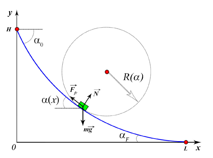
Let’s consider a small physical body, (a particle, material bead) of mass sliding down along some differentiable curve (thin rigid wire) specified by an explicit equation: . The classical laws of Newtonian mechanics make it possible to calculate the modulus of the sliding speed of the particle at any point of the trajectory, if we take into account changes of potential energy in the gravity field and the work of friction forces over the entire previous section of motion. The elementary work of the Coulomb friction force through the infinite small displacement can be expressed through the friction coefficient ; normal reaction and the friction force , which in its turn depends on the curvature radius of the trajectory at a given point of view (see Fig. 1).
Explicitly, the modulus of the elementary work of the friction force can be written as follows:
| (1) |
The inclination angle of the trajectory at the observation point (see Fig. 1) is introduced in eq. (1). It can be calculated through the first derivative of the descent curve function: :
| (2) |
It will be convenient to express the sliding speed in terms of the horizontal projection of the velocity vector using the relation:
| (3) |
Here, as usual, the prime at the function indicates its derivative with respect to -variable, when the dot indicates the derivative with respect to time. The curvature radius of the trajectory is expressed through the first and second derivatives of the sliding function :
| (4) |
Substituting formulas (3), (4) into (1), we obtain the expression for the friction force work through the infinitesimal displacement along the trajectory:
| (5) |
The total work of resistance forces can be calculated by integrating formula (5) over changes in horizontal -coordinate from zero to the current location of the particle.
| (6) |
In the resulting formula, an auxiliary function has been introduced which is equal to the square of the horizontal projection of the velocity vector, expressed through the current -coordinate:
| (7) |
Using the law of changes in the kinetic energy of a sliding particle along the chosen trajectory and taking into account the work of the friction forces (6), we arrive at the following expression:
| (8) |
Reducing both sides of formula (8) by mass and passing with the help of (2) and (3) to the -speed square function (7), we transform (8) into the following integral equation:
| (9) |
Differentiating both sides of formula (9) with respect to the -variable, we obtain the first-order linear differential equation for the function:
| (10) |
Formula (10) was obtained in our work [9] directly from the Newton’s laws of dynamics, where a general solution to this equation in quadratures was also found for an arbitrary twice differentiable descent curve :
| (11) |
The “acceleration history” function satisfying the initial conditions is introduced in equation (11). The initial conditions imply that , so the function can be written through the following integral:
| (12) |
Then the total descent time along a given trajectory can be found by integrating the function (11) along the horizontal coordinate.
| (13) |
Formulas (11) - (13) were used in our papers [9, 11] to calculate the sliding time along parabolas and the cycloid taking into account the Coulomb friction forces. In this article we make an attempt to find the equation of the fastest descent curve (brachistochrone) for a given value of the friction coefficient . Let us seek the equation of brachistochrone in the following parametric form:
| (14) |
where is some unknown dimensionless function that determines the shape of the brachistochrone. Parameter is a scale factor having the dimension of length, is another free parameter corresponding to the initial inclination angle for the slip curve at the point . Equations (14) define the brachistochrone in parametric form, as a function of the angle parameter which corresponds to the inclination of the curve graph with respect to the -axis (see Fig. 1). It is assumed that the brachistochrone is a curve with positive curvature (4), for which the slope angle should monotonically decrease from some initial value to the final smaller one , so that the region is under consideration . This idea has been suggested by numerical calculations for the descent time along parabolas with different signs of curvature [10]. This statement is also confirmed by the cycloid equation, which is the curve of the fastest descent when . The parametric equations of the cycloid
can be rewritten in a similar form:
| (15) |
which corresponds to the choice in formulas (14). In this case, the “time” parameter in the cycloid is related to the slope of the cycloid graph by simple relationship:
| (16) |
The limiting value of -variable included in the cycloid equations (15), (i.e. is associated with the final steepness of the cycloid at the point
Exact values of parameters for the cycloid equations (15) can be calculated from following system of equations which relates them to the Cartesian coordinates of the beginning and ending points and :
| (17) |
The solution to this system which we name the boundary conditions can be obtained only numerically. For example, the choice of the initial data corresponds to the following values in the SI system [8]:
| (18) |
When friction forces are taken into account the parameters included in the brachistochrone equations (14) must also obey some boundary conditions similar to that of transcendental system (17). Thus, we arrive to the following equations:
| (19) |
| (20) |
Substituting parametric equations of the supposed brachistochrone (14) into (11) – (13) we get the expression for the total descent time, written as an integral of some unknown function :
| (21) |
In this case, the “acceleration history” function (12) transforms with constant multiplier to the dimensionless integral of the same function , which is also included in eq. (21) through the following modification
| (22) |
From a mathematical point of view, the problem of finding the fastest descent curve (brachistochrone with friction) has been reduced to finding the minimum value of the functional (21) by choosing a “suitable” function and the corresponding parameters with restrictions (19), (20). Now we can talk more specifically about different approaches to solving the problem of brachistochrone with Coulomb friction. In the work [3] and subsequent publications, the problem of finding the extremum of functional (21) was combined with boundary conditions (19) - (20), which led to very complex equations. The authors were unable to solve these equations analytically and find adequate formulas for brachistochrone with friction. In this article, we propose first to find the shape of the extremal curves for functional (21), and then, by choosing the optimal parameters ensure that boundary conditions (19) - (20) are met. This idea was suggested by analytical and numerical calculations of the sliding time along a cycloid in the presence of dry friction force [9]. Note that at zero friction , if the cycloid equations (15) are substituted into (21), (22) then the integrand in formula (21) becomes a constant and does not depend on the inclination angle of the trajectory at a given point. Thus, the time of descent is determined only by the parameters :
| (23) |
Let us use this condition as a criterion for finding the minimum value of the functional (21), because if the integrand is a constant then its variation will be equal to zero as must be for the extremum value. We suppose that the shape of the desired brachistochrone is determined by the condition:
| (24) |
The choice of the constant number ”-1” in the right side of formula (24) is quite arbitrary and can always be changed by redefining the scale factor . Then the time of descent along the optimal curve will depend only on the scale parameter and the inclination angles of the curve at the initial and final points of the trajectory , .
| (25) |
Relationship (24) is equivalent to the following integral equation:
| (26) |
We differentiate both sides of equation (26) with respect to the variable and get:
| (27) |
Solving this first-order linear differential equation with the initial condition , (which corresponds to the zero initial speed , we obtain the formula:
| (28) |
Note that the choice which was made in papers [3, 5] because is not justified and erroneous from our point of view. The initial inclination angle of the trajectory is also determined by the friction coefficient and will be calculated below. Substituting (28) into formulas (14) we obtain a parametric form of the desired brachistochrone with Coulomb friction forces:
| (29) |
where
| (30) |
| (31) |
Since the formulas (2), (2) turned out to be quite cumbersome, let us rewrite them in trigonometric form, using the critical friction angle . As known, downward sliding without an initial speed is possible only if the inclination angle of the trajectory is greater than it ( .
| (32) |
In this form of notation, equations (28) – (2) take the form:
| (33) |
| (34) |
| (35) |
Now we proceed to finding other free parameters , , of the brachistochrone minimizing the value of the functional (21) with boundary conditions (19), (20). Once the shape of the optimal curve is found the problem reduces to calculate the extremum value of the function (25):
| (36) |
with boundary conditions that follow from (19), (20):
| (37) |
Let us use the standard Lagrange method with multipliers and consider the auxiliary Lagrange function combining formula (36) and restrictions (37):
| (38) |
Partial derivative of the Lagrange function (38) with respect to variable gives the first equation for the extremum point:
| (39) |
Other partial derivatives with angles , produce a system of linear equations:
| (40) |
where the elements of the system matrix have the form:
| (41) |
Solving the system (40) we find the Lagrange multipliers :
| (42) |
where is the main determinant of the system:
| (43) |
Substituting the found solutions (42) into the first extremum equation (39) we find the sought interrelation between the initial and final slope of the brachistochrone graph with friction coefficient .
| (44) |
The determinant of the system of linear equations (40) after substitution formulas (2), (2) into equation (43) takes the form
| (45) |
The required relationship between and which we obtain from eq. (44) with the aid of (2), (2), (2) after simple but rather cumbersome transformations can be written as follows
| (46) | |||
In spite of quite complicated form of this equation, it can be easily analyzed by computer methods. For numerical calculations, the “Mathcad” program was used, the worksheet code in which can be viewed in the Internet via a link to the author’s website [12]. It is also noteworthy that at zero friction the equation (2) takes the simplest form:
| (47) |
from which it follows that , as is true for the cycloid (15). However, when friction forces are taken into account, the initial and final inclination angles of the brachistochrone graph , are related to the sliding friction coefficient and the parameters of the problem by a combined system consisting of equation (2) and the formula resulting from relations (37):
| (48) |
3 NUMERICAL ANALYSIS
Let us now carry out a numerical analysis of the obtained expressions, comparing the time of movement along the found brachistochrone and the cycloid at different values of the friction coefficient . We choose the parameters of the problem in accordance with the previously considered slide profile (18):
| (49) |
All reasoning carried out above shows that there is no universal curve that provides the minimum descent time for an arbitrary value of the friction coefficient . We can only talk about a family of curves, the shape of which also depends on the friction coefficient. Figure 2 shows three such curves given by formulas (29), (2), (2) for some different values of the friction coefficient
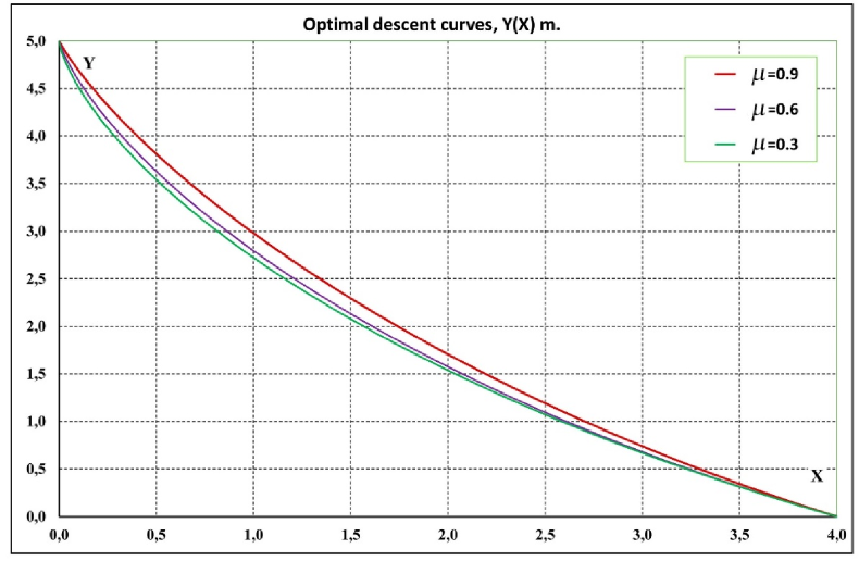
For the given parameters of the problem (49), these curves do not differ very much from each other and are externally similar to the cycloid [8], into which they degenerate at . The descent time along the family of these curves (proposed brachistochrones) (2), (2) for different values of the friction coefficient is shown in Fig. 3. Here, for comparison, we also depict the time of descent along the cycloid (15) and along the parabola (50) with the curvature parameter , which was also considered in our previous work [9].
| (50) |
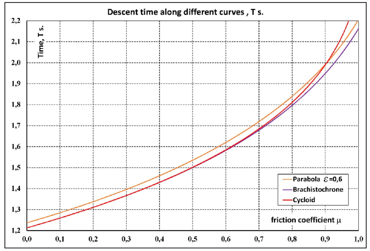
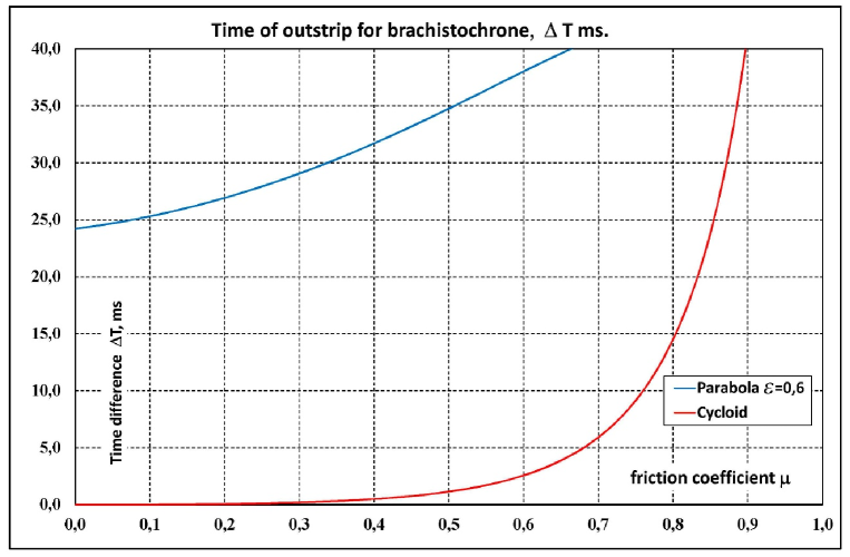
These graphs show that up to the values, the differences between the family of the curves (29), (2), (2) and the cycloid (15) are practically unnoticeable. The particle on the proposed brachistochrone outstrips the one on the cycloid in descent time about some milliseconds, which is clearly illustrated in Fig. 4. So, numerical calculations show that the family of the above-mentioned curves (29) – (2) can claim to be the brachistochrone for a given sliding friction coefficient. Numerical experiments with other initial data of the problem, different from (49), show that this statement remains valid and the family of curves (2), (2) provides the minimum descent time for a given value. It is curious to state that in the case which was analyzed in [3, 5] a particle on the cycloid is not able to finish and stops somewhere halfway if the friction coefficient is greater than the value . This occurs because of the condition implying fast acceleration and great increase of the friction forces on the rather curved trajectory. At the same time the particle on the brachistochrone (29)-(2) with is able to slide to the finish line up to the values .
Numerical analysis of formulas (2), (48) allows us to trace the dependence of the initial and final inclination angles of the brachistochrone graph (29) on the friction coefficient . The calculation results are shown in Fig.5.
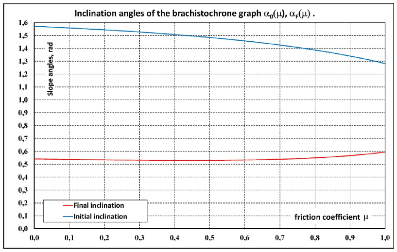
As can be seen from the graphs in Fig.5, the initial slope angle monotonously decreases from value to value with the increase of sliding friction coefficient , i.e. changes by approximately 18%. As for the final slope of the brachistochrone graph , it increases by approximately 9% from the value to . Thus, with an increase in the sliding friction coefficient, the brachistochrone graph straightens more and more and the radius of the average curvature of the trajectory becomes larger. This is clearly seen from Fig.2 and has a simple physical explanation. The sliding friction forces decrease at high speed on a less concave trajectory, so the steep initial section of brachistochrone with fast acceleration smoothly transitions into a less concave section of almost straight finish.
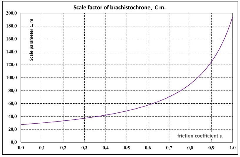
The scale parameter of the fastest descent trajectory (29) can be calculated from formulas (37) through the initial data of the problem (49) and the found angles of initial and final steepness. This value turns out to be strongly dependent on the friction coefficient. Figure 6 shows how the scale factor changes with the increase of . The initial value grows up more than seven times and reaches the magnitude at .
Let us now discuss the geometric and physical meanings of function (28), (33) that defines the brachistochrone equation in parametric form (14). Using formula (4), we can find the interrelation between this function and the curvature radius of the trajectory at a given location:
| (51) |
For a cycloid, and this formula takes the simplest form:
| (52) |
On the other hand, the function can be associated with the horizontal projection of the body velocity on curve (14), using formulas (7), (11), (22)
| (53) |
Taking into account the condition (26), the last formula can be written in terms of the magnitude of the velocity vector in the form:
| (54) |
On the cycloid (15), the relation (54) has the form of the well-known optical-geometric formula for the change in the speed of light when passing through a medium with a variable refractive index:
| (55) |
As is known, it was this optical-mechanical analogy that led Bernoulli to his solution to the problem of the frictionless brachistochrone [1]. An interesting relation follows from formulas (52) and (55)
| (56) |
This formula was used in the papers [13, 14] and led the authors to the idea that even in the presence of the Coulomb friction forces, this equation connecting the speed of the particle with the curvature radius should be satisfied on the true brachistochrone. Note that our calculations indicate that relation (56) is not satisfied on the brachistochrone (2), (2) and the following formula takes place instead:
| (57) |
The physical meaning of this formulas (56), (57) is quite clear: the closer a particle on the brachistochrone moves to the finish line, the flatter its trajectory should be in order to reduce the value of the friction force associated with the curvature of the trajectory. For the cycloid, both formulas (56), (57) are satisfied, and only calculating the descent time makes it possible to find out which of the proposed curves can claim the title of brachistochrone with friction (see [14]).
We use formulas (33) and (54) to calculate the velocity of a particle on the brachistochrone (29) - (2) and find:
| (58) |
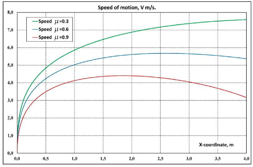
This relation generalizes Bernoulli’s formula (55) to the case of sliding with non-zero friction under the additional condition, that and it is calculated separately. Figure 7 illustrates how the speed on the generalized brachistochrone (29) – (2) changes when the particle moves and horizontal -coordinate increases from the start to final the value . Three curves with different friction coefficients as in Fig. 2 and with the same initial data (49) were analyzed. As can be seen from the Fig. 7, when there appears sections with braking and velocity decrease. So the particle rapidly loses its kinetic energy and may even stop before reaching the finishing coordinate: . The critical value of the friction coefficient at which the movement is still possible for this case is equal to .
4 CONCLUSION
In this work, we studied motions of a small physical body (massive particle) along a family of some curves taking into account the Coulomb friction forces. It was found that these curves provide the minimum descent time of sliding with friction and can claim the title of brachistochrone generalizing the cycloid equation for this case. We have obtained new formulas for such optimal curves (29) - (2) which depend on the initial parameters of the problem and the friction coefficient in two ways explicitly and through three implicit monotonic functions , allowing only numerical analysis (37), (2), (48). It is argued that the initial slope of the brachistochrone couldn’t be equal to that one of the cycloid for all values of the friction coefficient and contrary to the widely used opinion the statement is affirmed. The equations of the proposed brachistochrone with friction, make it possible to calculate the descent time at a given value of friction coefficient and compare it with the sliding time along other curves. Table 1 shows the results of such calculations for an isosceles profile , where the descent time (21) is expressed in dimensionless relative units, which makes it possible to exclude the scale factor of such movement. For this, the following formula was used (see also [7]):
| (59) |
| Circle | Parabola | Cycloid | Curve | Brachistochrone | |
| (50), =0,6 | (15) | (17) from [14] | (29)-(2) | ||
| 0,0 | 2,62206 | 2,66174 | 2,58190 | 2,58190 | 2,58190 |
| 0,1 | 2,75010 | 2,78825 | 2,70362 | 2,70455 | 2,70355 |
| 0,2 | 2,89716 | 2,93102 | 2,83995 | 2,84519 | 2,83961 |
| 0,3 | 3,07126 | 3,09421 | 2,99536 | 3,01354 | 2,99424 |
| 0,4 | 3,28824 | 3,28381 | 3,17686 | 3,23534 | 3,17372 |
| 0,5 | 3,58913 | 3,50894 | 3,39668 | 3,83072 | 3,38817 |
| 0,6 | 4,28398 | 3,78472 | 3,67962 | - | 3,65532 |
| 0,7 | - | 4,13991 | 4,09366 | - | 4,01019 |
| 0,8 | - | 4,64714 | - | - | 4,53711 |
| 0,9 | - | - | - | - | 5,53458 |
The dashes in this table indicate that the particle on this curve cannot reach the finish line and stops somewhere in the middle part of the trajectory, wasting the initial potential energy on the work against friction forces. The penultimate column of the table also shows calculations using formula (17) from the paper [14], in which the author used hypothesis (56) for a brachistochrone with friction. Note that the formulas (19) from the same work, obtained using the law of energy conservation are incorrect in the presence of friction forces and therefore were not used in our calculations.
Comparing the data obtained, one can be convinced that curves (29) - (2) really provide the minimum descent time and the hypothesis (56) is unfounded in the presence of friction forces. In addition, from formula (57) it follows that
| (60) |
Thus, the particle on the brachistochrone moves in such a way that over time the rate of change in the inclination angle of its trajectory relative to the horizontal -axis remains constant. The condition (60) is satisfied both in the absence of sliding friction force and in the presence of the latter.
References
- [1] Tikhomirov V.M. Stories about maxima and minima, vol. 1 of Mathematical World, Universities Press, 1990, 200 p.
- [2] Courant R., Robbins H. What Is Mathematics? An Elementary Approach to Ideas and Methods, Oxford University Press, 1996, 592 p.
- [3] Ashby N., Brittin W.E., Love W.F., Wyss W. Brachistochrone with Coulomb friction // American Journal of Physics, 1975, 43, 902-906; https://doi.org/10.1119/1.9976
- [4] Hayen J.C. Brachistochrone with Coulomb friction // International Journal of Non-Linear Mechanics, 2005, 40, 1057–1075; https://doi.org/10.1016/j.ijnonlinmec.2005.02.004
- [5] Sumbatov A.S. Brachistochrone with Coulomb friction as the solution of an isoperimetrical variational problem // Int. J. Non-Linear Mech. 2017. V. 88. P. 135–141. https://doi.org/10.1016/j.ijnonlinmec.2016.11.002
- [6] Lipp S.C. Brachistochrone with Coulomb friction, SIAM J. Control Optim. 1997, 35 (2), 562 –584.
- [7] Barsuk A.A., Paladi F. On parametric representation of brachistochrone problem with Coulomb friction // Int. J. Non-Linear Mech. 2023, V. 148, 104265, https://doi.org/10.1016/j.ijnonlinmec.2022.104265
- [8] Kurilin A.V. Employing the Mathcad program within the course of Theoretical Mechanics // SHS Web Conf., Volume 29, 2016, 2016 International Conference “Education Environment for the Information Age” (EEIA-2016), 02025, p.3, http://dx.doi.org/10.1051/shsconf/20162902025
- [9] Kurilin A.V. Brachistochrone and Sliding with Friction // arXiv:2305.18345 [physics.class-ph], http://dx.doi.org/10.48550/ARXIV.2305.18345
- [10] Kurilin A.V. Brachistochrone and non-integrable problems of analytical mechanics // Methodological issues in teaching infocommunications in higher education, 2023, Vol. 12, No. 1, pp. 55-61.
- [11] Kurilin A.V. Brachistochrone and sliding taking into account the force of friction, // Proceedings of the XVIII International Industrial Scientific and Technical Conference ”Technologies of the Information Society”, M.: Media Publisher , MTUCI, 2024, pp. 173-176.
- [12] Kurilin A.V. Virtual physical experiments and modeling of mechanical phenomena using the Mathcad program // Proceedings of the X International Scientific and Practical Conference “Educational Environment Today and Tomorrow”, M.: 2015, MTI Publishing House, pp. 382-385. http://mgopu-math.narod.ru
- [13] Gladkov, S.O., Bogdanova, S.B. Analytical and Numerical Solution of the Problem on Brachistochrones in some General Cases.// J. Math. Sci. 2020, V. 245, 528–537. https://doi.org/10.1007/s10958-020-04709-0
- [14] Gladkov S. O. Exact Solution of the Problem of Brachistochrone with Allowance for the Coulomb Friction Forces. // Tech. Phys. Lett. 2023 V. 49, 26–-28. https://doi.org/10.1134/S1063785023040016