FAAGC: Feature Augmentation on Adaptive Geodesic Curve Based on the shape space theory

Abstract

Deep learning models have been widely applied across various domains and industries. However, many fields still face challenges due to limited and insufficient data. This paper proposes a Feature Augmentation on Adaptive Geodesic Curve (FAAGC) method in the pre-shape space to increase data. In the pre-shape space, objects with identical shapes lie on a great circle. Thus, we project deep model representations into the pre-shape space and construct a geodesic curve, i.e., an arc of a great circle, for each class. Feature augmentation is then performed by sampling along these geodesic paths. Extensive experiments demonstrate that FAAGC improves classification accuracy under data-scarce conditions and generalizes well across various feature types.

1 Introduction

Using deep neural networks to extract and transform features has become a mainstream approach for various data modalities and downstream tasks. However, data scarcity remains a significant challenge, particularly in specialized fields such as medical imaging and materials science. Data augmentation strategies have been specifically designed for particular datasets and tasks, often requiring guidance from domain experts. This variability in augmentation strategies limits the model’s generalizability during training and preprocessing. For example, flipping or rotating images of animals in natural photographs does not alter semantic meaning, making them suitable for augmentation. However, such methods are unsuitable for tasks involving traffic signs, etc.. In medical or material images, domain knowledge is required to ensure augmentations do not alter semantic content.

Representation augmentation, offers a resource-efficient alternative to image-level augmentations due to its lower dimensionality and broader applicability across domains. While prior work has explored representation augmentation, issues such as poor interpretability and unclear optimization objectives have hindered its adoption and effectiveness.

To address these issues, we propose a novel data augmentation method based on the shape space theory Han et al. (2010). In the pre-shape space, objects with the same shape lie on a great circle. Assuming that features extracted by deep learning models capture critical information, we project these representations into the pre-shape space and adaptively construct a geodesic curve for each class. This geodesic corresponds to a segment of the great circle. While learning the geodesic, we also optimize the sampling parameters to ensure that the geodesic fits the sample points effectively, allowing for feature sampling along it for augmentation.

After learning the geodesic and sampling parameters, we sample features from the geodesic to augment the dataset and train the classifier jointly with the original samples. We conduct experiments on image datasets with various mainstream deep learning backbones and adjust the number of training samples per class to validate the method’s robustness under limited data conditions. The results demonstrate that our method significantly improves classification accuracy under limited training samples. Furthermore, our ablation studies show that our proposed method is independent of traditional image-based augmentation techniques and can further enhance classification accuracy when combined with them.

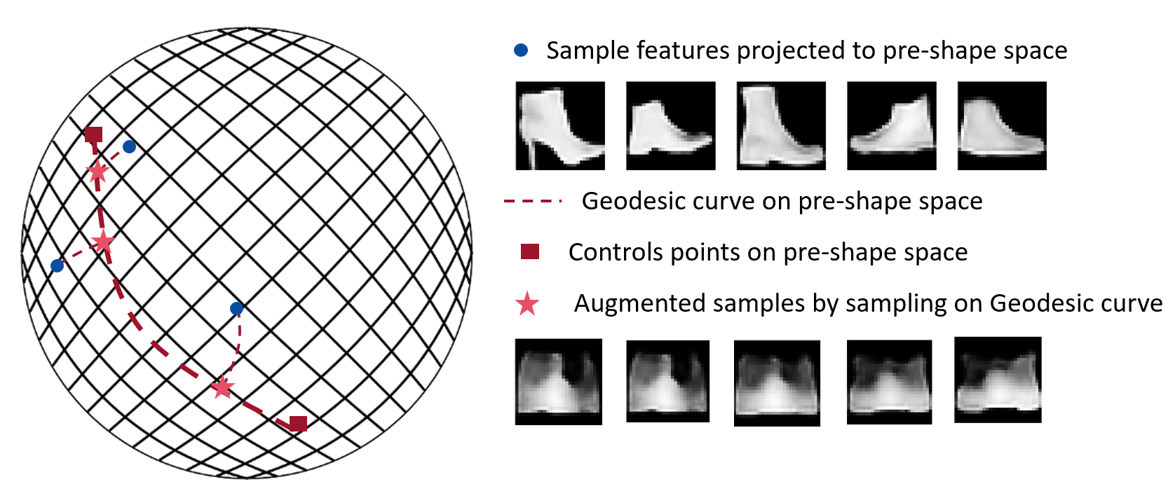
Figure 1: Illustration of the FAAGC. The top-right images show samples decoded from the pre-shape space using a VAE model trained on Fashion-MNIST. The bottom-right images show FAAGC-augmented samples decoded from the same space.

2 Related Works

2.1 Input-Level Data Augmentation

Due to challenges such as data scarcity, annotation difficulties, and distribution biases across different modalities, researchers in various fields have proposed diverse data augmentation methods to enhance the generalization and robustness of models.

In the image domain, commonly used data augmentation techniques include flipping, rotation, translation, scaling, noise addition, occlusion, and color jittering. They increase the diversity of training image samples, and improve generalization capability Shorten and Khoshgoftaar (2019). In Natural Language Processing (NLP), strategies such as synonym replacement, word deletion, and sentence fragment swapping are employed to generate diverse data from limited or imbalanced corpora, thereby enhancing performance in tasks like text classification and sentiment analysis Wei and Zou (2019).

For high-precision scenarios like medical imaging analysis, data augmentation involves generating synthetic samples using Generative Adversarial Networks (GANs), simulating realistic lesion characteristics, creating rare case images, and augmenting CT and MRI data with specific slice augmentations. These methods significantly enhance data diversity and model robustness Frid-Adar et al. (2018).

While GAN-based augmentation can be effective, it becomes challenging when sample sizes are very limited due to its reliance on abundant data for stable training. Insufficient samples often lead to issues like mode collapse or overfitting, hindering the generation of high-quality synthetic data Karras et al. (2020). In specialized fields such as medicine, both general-purpose and domain-specific data augmentation methods can be utilized to enhance task performance Athalye and Arnaout (2023).However, these augmentation methods require validation through dataset-specific experiments and the acceptance of domain experts to ensure their applicability and effectiveness.

2.2 Feature-Level Data Augmentation

Feature-based data augmentation, which leverages representations extracted by deep learning models, offers advantages in enhancing data diversity and improving model robustness.

Goodfellow et al. Goodfellow et al. (2014) introduced adversarial examples as a tool to explore model vulnerabilities and laying the groundwork for feature manipulation in data augmentation. Terrance DeVries DeVries and Taylor (2017) proposed augmenting data through Variational Autoencoders (VAEs) Kingma (2013) that map image samples into a latent space, where extrapolation, interpolation, and perturbation methods are applied to produce diverse data. Vikas Verma introduced Manifold Mixup Verma et al. (2019), to enhance robustness and accuracy against adversarial examples by mixing feature representations. P. Li demonstrated that simple feature augmentation in transfer learning can significantly improve model generalization and robustness Li et al. (2021b). Li et al. Li et al. (2021a) also proposed MoEx, which disrupts the mean and variance of image features with those of other samples to create new examples, making the method independent of specific modalities. Peng Chu enhanced long-tailed dataset performance with feature-level augmentation Chu et al. (2020), and Dan Liu applied SMOTE to feature spaces, expanding fault samples in gas turbine datasets and improving model performance Liu et al. (2024).

The above discussed methods differ significantly in implementation but share a common workflow for data augmentation. They can be summarized as follows: given a training dataset $\mathcal{D}_{\text{train}}=\{X,y\}$, where $X$ represents the input to the deep model, such as preprocessed image data, and $y$ denotes the corresponding labels. Deep feature extraction is first performed using a feature encoder, resulting in high-dimensional, modality-independent representations $X_{\text{enc}}=f_{\text{enc}}(X;\theta_{\text{enc}})$. $\theta_{\text{enc}}$ represents the learnable parameters of the deep learning model used for feature extraction. Next, an augmentation algorithm $f_{\text{aug}}$ is applied to produce the augmented dataset $\mathcal{D}_{\text{aug}}=(X_{a},\tilde{y}_{a})=f_{\text{aug}}(X_{\text{enc}},y)$. Here, $X_{a}$ denotes the augmented features generated by the augmentation algorithm, and $\tilde{y}_{a}$ represents the pseudo-labels corresponding to these features. The augmentation function $f_{\text{aug}}$ generally depends on $X_{\text{enc}}$ and $y$, but it may also include additional parameters. For example, the Fast Gradient Sign Method (FGSM) Goodfellow et al. (2014) incorporates the classifier parameters $\theta_{\text{classifier}}$.

Feature-level data augmentation methods effectively enhance data diversity and model robustness by manipulating learned feature representations through techniques like adversarial perturbations, latent space interpolations, and feature mixing. However, these methods often rely on linear transformations or distribution-based sampling, which may overlook the complex geometric structures of data and fail to preserve intrinsic relationships between samples. This can result in less effective augmentation, particularly when semantic consistency is crucial. To address the limition, introducing shape space theory offers a promising solution by modeling data in a geometry-aware manner. Projecting features into pre-shape space and applying geodesic-based transformations enables the generation of more diverse and semantically meaningful samples, overcoming the shortcomings of traditional feature-level augmentation.

2.3 Introduction to Shape Space Theory

The theory of shape space, introduced by Kendall, is used to describe objects and their equivalent transformations in non-Euclidean space. Shape space ignores translations, scaling, and rotations of objects, focusing instead on representing their intrinsic shape features Kendall (1984). This theory is often applied to object recognition, where the distance between objects in the shape space determines recognition outcomes.

To enable computational representation and analysis, object shapes are first projected into the pre-shape space, denoted as $S_{*}^{2d-3}$. For a feature $x$ of dimension $d$, the corresponding formula is:

$$K_{S}(x)=\frac{(x_{1}-\bar{x},\,x_{2}-\bar{x},\,\ldots,\,x_{d}-\bar{x})}{s(x)},$$ (1)

$$\bar{x}=\frac{1}{d}\sum_{j=1}^{d}x_{j},\quad s(x)=\left(\sum_{j=1}^{d}\|x_{j}-\bar{x}\|\right)^{1/2}.$$

The function $K_{S}(x)$ represents the projection of a feature $x$ into the pre-shape space by normalizing it with respect to its mean $\bar{x}$ and scale $s(x)$.

In the pre-shape space, shape variations such as position, scale, and rotations correspond to great circle paths $O(v)$ on a hypersphere. The set of all such transformations forms the orbit space $\Sigma_{2}^{d}$, defined as:

$$\Sigma_{2}^{d}=\{O(v):v\in S_{*}^{2d-3}\}.$$ (2)

The set of all points on the great circle can be used to represent a specific shape. In the pre-shape space $S_{*}^{2d-3}$, the geodesic distance between two points is equivalent to the great circle distance on the manifold. For two feature points $v_{0}$ and $v_{1}$ in the pre-shape space $S_{*}^{2d-3}$, their geodesic distance is defined as the great circle distance Kendall et al. (2009):

$$g_{K_{s}}(v_{0},v_{1})=\arccos{\langle v_{0},v_{1}\rangle},$$ (3)

where $g_{K_{s}}(v_{0},v_{1})$ is the geodesic distance between $v_{0}$ and $v_{1}$ in the pre-shape space, and $\langle v_{0},v_{1}\rangle$ denotes their inner product.

It is difficult to obtain feature positions in the shape space. Instead, the distance in shape space, denoted as $g_{K}$, can be computed as the shortest geodesic distance between the great circles associated with the projections of two features in the pre-shape space, expressed as:

$$g_{K}(v_{0},v_{1})=\inf g_{K_{s}}(O(v_{0}),O(v_{1})).$$ (4)

This distance can quantify the similarity of key objects between two images based on the geodesic distance between key points Han (2013).

By constructing a geodesic curve between two points in the pre-shape space $S_{*}^{2d-3}$, new data points within the pre-shape space can be generated. For example, given two points $v_{0}$ and $v_{1}$ in $S_{*}^{2d-3}$, intermediate points along the geodesic curve can be generated using the following formula:

$$\Gamma_{(v_{0},v_{1})}(s)= (\cos s)\cdot v_{1}+(\sin s)\cdot\frac{v_{1}-v_{0}\cdot\cos g_{K_{s}}(v_{0},v_{1})}{\sin g_{K_{s}}(v_{0},v_{1})},$$ (5)

$$\quad(0\leq s\leq\theta_{(v_{0},v_{1})}).$$

where $g_{K_{s}}(v_{0},v_{1})$ denotes the geodesic distance between $v_{0}$ and $v_{1}$, and $s$ represents the angle along the geodesic curve. Based on this approach, a geodesic curve can be constructed in the pre-shape space to fit features from multiple images and generate new features along the curve for feature augmentation.

Applications of shape space in data generation include  Vadgama et al. (2022) using a VAE framework to generate samples on the MNIST dataset by representing the latent space as shape space, and projecting deep learning features into the pre-shape space for data augmentation.  Han et al. (2023) proposed the GCFA framework, which projects deep learning features as key points into the pre-shape space and performs data augmentation to improve learning efficiency and classification accuracy in low-data scenarios. These approaches highlight the potential of shape space theory in enhancing data augmentation, especially for low-resource tasks across various domains.

3 Method

3.1 Notation

In the pre-shape space, points are denoted as $v_{0},v_{1}\in S_{*}^{2d-3}$. For their corresponding points in the Euclidean space, the notation $v_{0}^{R},v_{1}^{R}\in\mathbb{R}^{d}$ is used, where the $R$ indicates the Euclidean space. Class labels are denoted by $y$, with $y\in\{1,2,\dots,C\}$, where $C$ represents the total number of classes. Additionally, pseudo-labels are represented as $\tilde{y}$.

3.2 Feature Augmentation on Adaptive Geodesic Curve

Feature Augmentation on Adaptive Geodesic Curve leverages a segment of a great circle in the pre-shape space to represent the shape of a sample class and performs data augmentation by sampling feature points along this great circle. The method aims to identify the optimal segment of the great circle that best represents the sample points, which involves determining the two optimal endpoints of the segment. The workflow of this augmentation and representation enhancement is illustrated in Fig. 2.

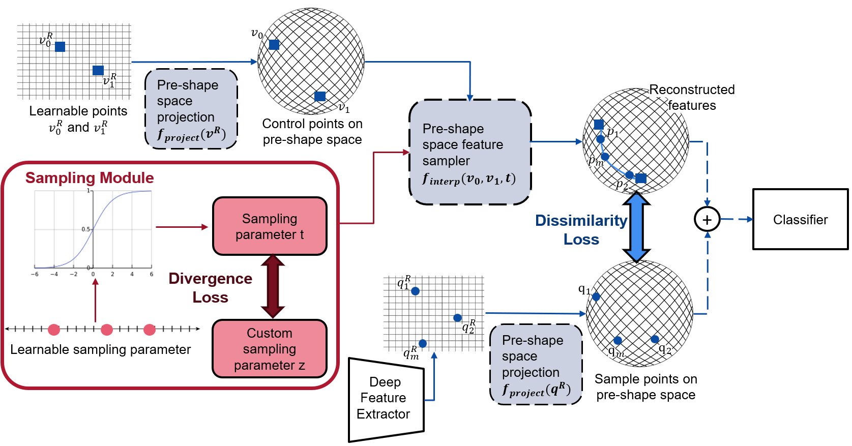
Figure 2: Workflow of Feature Augmentation on Adaptive Geodesic Curve(FAAGC).

Given two randomly initalized points $v^{R}_{0}$ and $v^{R}_{1}$ in $\mathbb{R}^{d}$, they are first projected into the pre-shape space using the projection function 1, denoted as $v_{0}$ and $v_{1}$, respectively.

To generate augmented data points, a distribution restricted to $[0,1]$ is required, and in this work, a uniform distribution $U(0,1)$ is used for its simplicity. Using these sampled values, augmented points in the pre-shape space are obtained through the interpolation formula, with Function 6.

$$a=f_{\text{interp}}(v_{0},v_{1},z)=\frac{\sin\left[(1-z)\theta\right]}{\sin\theta}v_{0}+\frac{\sin\left(z\theta\right)}{\sin\theta}v_{1}$$ (6)

This formula is equivalent to formula 5 when implemented with given $v_{0}$, $v_{1}$, and the sampling parameter $z$ in $[0,1]$. While, $\theta=\arccos\left(v_{0}^{\top}v_{1}\right)$ represents the geodesic distance $v_{0}$ and $v_{1}$. Our objective is to ensure that the augmented point $a$ aligns as closely as possible with the distribution of the original data points. This is achieved by maximizing the log-likelihood:

$$\max_{v_{0},v_{1}}\mathbb{E}_{z\sim U(0,1)}\log p(a),\quad a=f_{\text{interp}}(v_{0},v_{1},z)$$ (7)

Inspired by the theoretical contributions of VAEs, we reformulate the process of maximizing the above log-likelihood into minimizing a weighted sum of two terms: the similarity loss between all sample points and generated points, and the divergence between the sampling distribution and the latent variable distributions $t$ and $z$, as follows:

$$\mathcal{L}=\sum_{i=1}^{m}\mathcal{L}_{\text{Sim}}(p_{i},q_{i})+\beta\cdot\mathcal{L}_{\text{Diverg}}(p(t)),p(z)).$$ (8)

The variable $t$ represents a set of $m$ values sampled from a learnable distribution, which is constrained to the range $[0,1]$. Similarly, $z$ is a set of $m$ values sampled from $U(0,1)$ used during data augmentation. Together with the learnable parameters $v_{0}$ and $v_{1}$ in the pre-shape space, $t$ is used to compute the sampled points $p_{i}$ ($i=1,\dots,m$) through the formula 6. Here, $m$ represents the number of samples projected into the pre-shape space. Each $p_{i}$ corresponds to a deep learning representation $q_{i}$. Specifically, $q_{i}$ is obtained by projecting the $q^{R}_{i}$, extracted and pooled by the deep model for the $i$-th sample, into the pre-shape space.

The reconstruction loss $\mathcal{L}_{\text{Sim}}$ measures the similarity between each pair of points $p_{i}$ and $q_{i}$, with higher similarity resulting in a smaller $\mathcal{L}_{\text{Sim}}$. Additionally, the divergence loss $\mathcal{L}_{\text{Diverg}}$ ensures the distribution $t$ aligns closely with the augmentation parameter $z$, with smaller divergence yielding a lower $\mathcal{L}_{\text{Diverg}}$. The hyperparameter $\beta$ balances the influence of the two loss terms.

For the loss term $\mathcal{L}_{\text{Sim}}$, the geodesic distance between $p_{i}$ and $q_{i}$ in the pre-shape space is defined as $\arccos(p_{i}^{\top}q_{i})$. To simplify computation, cosine similarity is used to measure their similarity, as shown in 9:

$$\sum_{i=1}^{m}\left(1-p_{i}^{\top}q_{i}\right)^{2}.$$ (9)

Given that we use a uniform distribution $U(0,1)$ for the sampling parameter, the divergence between distributions can be measured using the Wasserstein distance. Specifically, the Wasserstein distance can be approximated as

$$\frac{1}{m}\sum_{j=1}^{m}\left|t_{(j)}-z_{(j)}\right|,$$ (10)

where $t_{(j)}$ represents the $j$-th parameter in the sorted sequence of $m$ learnable latent variables $t$, and $z_{(j)}$ denotes the $j$-th parameter in the sorted sequence of $m$ samples drawn from the uniform distribution $U(0,1)$.

Therefore, the loss function can be reformulated as follows:

$$\mathcal{L}_{\text{train}}=\sum_{i=1}^{m}\left(1-p_{i}^{\top}q_{i}\right)^{2}+\beta\cdot\frac{1}{m}\sum_{j=1}^{m}\left|t_{(j)}-z_{(j)}\right|$$ (11)

The complete training process is outlined in Algorithm 1.

Algorithm 1 Geodesic Training Algorithm

0: Sample points for each class $Q^{R}_{c}=\{q^{R}_{1},\ldots,q^{R}_{m}\}$, hyperparameter $\beta$

0: Control points $v_{0},v_{1}$ in the pre-shape space for each class

1: for each class $c$ do

2:  Initialize $v^{R}_{0},v^{R}_{1}\in\mathbb{R}^{d}$ randomly, where $d$ is the feature dimension

3:  Initialize sampling parameters $\boldsymbol{t}=\{t_{1},\ldots,t_{m}\}$ with $t_{i}\sim\mathcal{N}(0,1)$

4:  Project control points to the pre-shape space: $v_{0}=f_{project}(v^{R}_{0}),v_{1}=f_{project}(v^{R}_{1})$ (see formula 1)

5:  Transform sampling parameters: $\boldsymbol{t}=\text{sigmoid}(\boldsymbol{t})$

6:  Sampling $P=\{p_{1},\ldots,p_{i},\ldots,p_{m}\}$ , $p_{i}=f_{interp}(v_{0},v_{1},t_{i})$ (see formula 6)

7:  Calculate similarity loss: $\sum_{j=1}^{m}\mathcal{L}_{Sim}$ (see formula 9)

8:  Sort $\boldsymbol{t}$ in ascending order to obtain $\{t_{(1)},\ldots,t_{(m)}\}$

9:  Sample a new set of parameters $\boldsymbol{z}=\{z_{1},\ldots,z_{m}\}$ from $U(0,1)$, and sort to obtain $\{z_{(1)},\ldots,z_{(m)}\}$

10:  Compute divergence loss: $\mathcal{L}_{div}$ (see formula 10)

11:  Set total loss: $\mathcal{L}=\sum_{j=1}^{m}\mathcal{L}_{Sim}+\beta\cdot\mathcal{L}_{div}$, and perform gradient descent to update $v_{0},v_{1}$, and $\boldsymbol{t}$

12: end for

13: return  $v_{0}$ and $v_{1}$ for each class

Initialization of the learnable parameters $v_{0}^{R}$ and $v_{1}^{R}$ can be performed using two approaches: sampling from a standard normal distribution $\mathcal{N}(0,I)$, or randomly selecting two distinct $q_{i}^{R}$ for initialization. In this paper, the latter method is employed for experiments. For the sampling parameters, we initialize them using a standard normal distribution and then apply the sigmoid function to ensure that the sampled values fall within the range $(0,1)$. It ensures that the sampling parameters are both valid and learnable during training.

Optimization is performed using the Adam optimizer with 2000 training epochs. The learning rates are set to 0.0003 for $v_{0}$ and $v_{1}$, and 0.003 for $t$. These rates were determined via grid hyperparameter search on the reduced CIFAR-100 training set (see Section 4.1) to effectively minimize the loss function and are applied consistently across all experiments.

The complete augmentation process, without additional adjustment to the weights of the augmented features, is described in 2.

Algorithm 2 Geodesic Data Augmentation Algorithm

0: Control points $v_{0},v_{1}$ in the pre-shape space for each class, desired augmentation size $n$, original training set $\mathcal{D}=\{(Q^{R}_{c},y_{c})\mid c\in\{1,2,\dots,C\}\}$

0: Combined dataset $\mathcal{D}_{\text{combined}}$, including original and augmented samples with labels

1: Project all points in $Q^{R}_{c}$ from Euclidean space to the pre-shape space using Formula 1, resulting in $Q_{c}$

2: Initialize augmented dataset $(X_{\text{aug}},\tilde{y}_{\text{aug}})=(\emptyset,\emptyset)$

3: for each class with label $c$ do

4:  Sample a batch of parameters $\boldsymbol{z}=\{z_{1},\dots,z_{n}\}$ from $U(0,1)$

5:  Generate augmented samples $X_{c}=\{x_{1},\dots,x_{n}\}$ using Formula 6, based on $v_{0}$, $v_{1}$, and $\boldsymbol{z}$

6:  Assign pseudo-labels $\tilde{y}_{c}=\{\tilde{y}_{1}=c,\dots,\tilde{y}_{n}=c\}$ for each $x_{i}\in X_{c}$

7:  Append $X_{c}$ and $\tilde{y}_{c}$ to the augmented dataset: $(X_{\text{aug}},\tilde{y}_{\text{aug}})\leftarrow(X_{\text{aug}}\cup X_{c},\tilde{y}_{\text{aug}}\cup\tilde{y}_{c})$

8: end for

9: Combine the original training set with the augmented dataset: $\mathcal{D}_{\text{combined}}=\mathcal{D}\cup(X_{\text{aug}},\tilde{y}_{\text{aug}})$

10: return  Augmented dataset $\mathcal{D}_{\text{combined}}$

To visualize the results of FAAGC-based augmentation, we trained a simple Variational Autoencoder on the Fashion-MNIST dataset  Xiao (2017) for reconstruction tasks. As shown in Fig 1, both reconstructed images without FAAGC and those with FAAGC lack texture details. However, the samples reconstructed using FAAGC effectively capture and visualize the diverse shapes of shoes from different orientations.

3.3 Comparison with Other Data Augmentation Methods

In the following sections, we compare our approach with the Variational Autoencoders (VAEs) and the pre-shape space augmentation framework GCFA, highlighting its advantages in scenarios with limited sample sizes.

3.3.1 Comparison with VAE

The loss function employed during the training of this method is conceptually similar to the loss function of VAEs Kingma (2013). However, in VAEs, the reconstructed sample $x_{recon}$ is generated by sampling $z\sim\mathcal{N}(0,1)$ and passing it through a parameterized conditional distribution $p(x|z;\theta)$. In contrast, our method performs uniform sampling along the great circle between two given sample points $v_{0}$ and $v_{1}$, generating intermediate points that lie between $v_{0}$ and $v_{1}$. These sampled points form a distribution that closely approximates the original data and carry explicit geometric significance, enhancing the performance of data augmentation, particularly in low-sample-size scenarios.

In VAEs, the optimization process involves constructing both the encoder $q(z|x;\phi)$ and decoder $p(x|z;\theta)$, which represent two parameterized conditional distributions. This approach enables the generation of diverse and high-dimensional samples but comes with high parameter complexity and computational cost during both training and sampling. In contrast, our method only requires optimizing two control points $v_{0}$ and $v_{1}$, along with the sampling parameter $t$. As a result, the number of parameters and computational resources needed for training and sample generation are significantly lower compared to VAEs.

Despite these advantages, a limitation of our method is its inability to perform one-shot data augmentation tasks, as it requires at least two sample points to learn and construct the geodesic. Addressing this limitation and extending the method to support one-shot tasks remains a focus for future work.

3.3.2 Comparison with GCFA

This method adopts a similar approach to GCFAHan et al. (2023) for data augmentation by utilizing control points in the pre-shape space and performing sampling along the great circle. Therefore, this method can be considered an improvement based on the GCFA data augmentation framework.

However, the two methods differ in how the optimal control points are determined. While GCFA employs an iterative distance calculation approach, our method uses a gradient descent algorithm. This makes our method significantly more efficient in terms of computation time during data augmentation compared to GCFA.

The following experiment demonstrate the training time differences between the two methods. A subset of the CIFAR-10 training set was used to select the optimal control points, with each class containing 5 or 10 sample points. The original samples were represented by features extracted using the ViT-t model. Both the GCFA method and the proposed method were applied for data augmentation, and the classification accuracy after data augmentation was evaluated using the same KNN classifier with $k=5$. The experiments were conducted on Intel(R) Xeon(R) Silver 4210R CPU. The experimental results are summarized as follows:

Method	Samples per Class	Training Time (s)	Accuracy (%)
GCFA	10	711.85	86.30
FAAGC	10	39.34	88.34
GCFA	5	351.83	85.20
FAAGC	5	39.39	85.84

Table 1: Comparison of Training Time and Classification Accuracy

The experimental results demonstrate that FAAGC achieves higher classification accuracy in data augmentation tasks while requiring significantly less computation time. This efficiency is primarily attributed to the use of low-complexity operations, such as transforming inner product calculations into Hadamard products followed by summation, and parallelizing absolute difference calculations. These optimizations enable higher parallelism and faster computation. In contrast, GCFA relies on computationally expensive operations, including extensive point sampling and geodesic distance calculations, resulting in longer runtime.

4 Experiments

4.1 Comparative Analysis

To evaluate the effectiveness of the FAAGC method for feature augmentation, we compare it with several existing feature augmentation techniques to validate its performance. The comparison includes a diverse range of representation augmentation methods. Specifically, we consider the following approaches: adversarial sample generation using FGSM Goodfellow et al. (2014), Manifold-Mixup Verma et al. (2019), SFA-S Li et al. (2021b), MoEX Li et al. (2021a), Feature-level SMOTE Liu et al. (2024), and GCFA Han et al. (2023).

Our experiments are conducted on the CIFAR-10, CIFAR-100, and CUB-200 datasets Krizhevsky et al. (2009); Wah et al. (2011), where the training sets are reduced to 5 samples per class to simulate a data-limited scenario. The full test sets are used to evaluate the generalization ability of the data augmentation methods. A pre-trained ViT-t model is fine-tuned independently on each dataset, and the extracted deep learning representations serve as the input for the data augmentation methods we mentioned. For the ViT-t model, the extracted feature dimension $d$ is 192.

Although FAAGC can generate an arbitrary number of augmented samples, we match the augmentation count with the original training data (5 samples per class) to ensure a fair comparison with other methods that may have constraints on the number of augmentations. The augmented features, along with the original features, are fed into the ViT-t classification head for retraining. During retraining, we follow the loss weighting strategy provided by GCFA, combining original and augmented data with specific weights in the loss function to optimize training:

$$\mathcal{L}=p_{g}\cdot\mathcal{L}_{\text{CE}}(y,\hat{y})+(1-p_{g})\cdot\left[\mathcal{L}_{\text{CE}}(y,\hat{y})+\lambda\cdot\mathcal{L}_{\text{CE}}(\tilde{y},\hat{\tilde{y}})\right],$$ (12)

where $p_{g}$ (set to 0.3) is the probability of using only the original data loss, $\lambda$ (set to 0.5) weights the augmented data loss, and $\mathcal{L}_{\text{CE}}$ represents the cross-entropy loss.

Method	CIFAR10	CIFAR100	CUB-200
No Augmentation	85.25$\pm$.00	66.41$\pm$.00	40.96$\pm$.00
FGSM	85.29$\pm$.03	66.33$\pm$.17	40.99$\pm$.04
Manifold-Mixup	81.11$\pm$.32	66.63$\pm$.10	40.99$\pm$.08
SFA-S	85.33$\pm$.03	65.26$\pm$.94	41.21$\pm$.04
MoEx	85.36$\pm$.04	66.25$\pm$.14	41.00$\pm$.02
Feature-level SMOTE	85.30$\pm$.03	66.41$\pm$.10	41.00$\pm$.07
GCFA	85.41$\pm$.03	66.39$\pm$.03	40.76$\pm$.04
FAAGC	86.04$\pm$.01	67.87$\pm$.04	41.15$\pm$.05

Table 2: Classification Accuracies of Different Augmentation Methods on diffent datasets

As shown in Table 2, our method improves classification accuracy under data-limited conditions across three datasets. Specifically, it increases accuracy from $66.41\%$ to $67.87\%$ on CIFAR-100, outperforms other class-based generation methods in Euclidean space, such as Feature-level SMOTE and MoEx, as well as the geodesic-based augmentation method GCFA in the pre-shape space. Similar improvements are observed on CIFAR-10 and CUB-200, as shown in the table.

To demonstrate the effectiveness of the proposed data augmentation method across various classifiers, we conducted comparative experiments using kNN, SVM, and MLP as classifiers alongside several augmentation methods, including SFA-S, MoEx, Feature-level SMOTE, and GCFA.

As shown in Table 3, FAAGC achieves significant performance improvements when using kNN, SVM, and MLP.

Method	kNN	SVM	MLP
No Augmentation	61.08	63.74	56.71
SFA-S	61.08	41.99	58.03
MoEx	61.60	64.44	57.52
Feature-level SMOTE	61.49	63.36	57.87
GCFA	62.57	63.48	65.02
FAAGC	62.92	65.01	64.57

Table 3: Classification Performance of Augmentation Methods across Different Classifiers

To demonstrate the effectiveness of the proposed method across various backbone networks for feature extraction, we applied FAAGC-based feature augmentation to subsets of the CIFAR-100 training set extracted using different backbone networks. The augmented features, together with the original features, were jointly used to retrain the classifier of the respective backbone network. The training setup remained consistent with the previous experiments. The backbone networks used in this evaluation include ResNet He et al. (2016), EfficientNet Tan and Le (2019), ViT Dosovitskiy et al. (2021), and Swin-Transformers Liu et al. (2021).

Method	Resnet	EfficientNet	ViT	Swin-Trans.
No Augment	38.26	35.99	66.41	59.71
FAAGC	39.52	36.48	67.87	61.28

Table 4: Classification Accuracy of Augmentation Methods across Different Backbone Networks

It can be observed from Table 4 that features extracted by various backbone models can be effectively enhanced using the FAAGC method. This enhancement leads to improved classification accuracy with limited sample availability.

The lower baseline accuracy of EfficientNet and ResNet backbones compared to ViT and Swin-Transformers is likely due to differences in the pretraining parameters we used. ResNet and EfficientNet were pretrained on the smaller ImageNet-1k, while ViT and Swin-Transformers used the larger ImageNet-21k and ImageNet-22k datasets.

We evaluated the effectiveness of data augmentation on the CIFAR-100 dataset as the number of samples per class gradually increased.

	3	5	10	20
No Augment	57.83	66.41	74.32	78.50
FAAGC	59.39	67.87	74.67	78.76

Table 5: Impact of Data Augmentation on Accuracy with Different Sample Sizes

The results in Table 5 show that the proposed data augmentation method consistently improves classification accuracy across different sample sizes. Notably, the performance gain is more significant when the number of samples per class is small. For instance, with only 3 samples per class, the accuracy improves from 57.83% to 59.39%. As the number of samples increases to 20, the improvement becomes marginal, increasing from 78.50% to 78.76%. This indicates that the proposed augmentation method is particularly effective in scenarios with limited data.

4.2 Ablation Study

Multiple ablation studies were conducted to validate the effectiveness and robustness of the proposed FAAGC method.

For the data augmentation process, an ablation experiment was performed on the CIFAR-100 dataset with 5 samples per class. The ViT-t model was used to extract input features, followed by three different augmentation strategies to evaluate the effectiveness of data augmentation: (1) direct classification without any augmentation, (2) classification after projection into the pre-shape space, and (3) classification after applying the complete FAAGC pipeline. A $k$-Nearest Neighbor (kNN) classifier with $k=5$ was used for all ablation experiments below.

The results from Table 6 confirm that the the complete FAAGC significantly enhances classification accuracy.

Pre-Shape Space Project	Geodesic Augment	Accuracy(%)
No	No	61.59
Yes	No	61.14
Yes	Yes	64.13

Table 6: Ablation Study on Geodesic Augmentation Process

Next, we conducted an ablation study on the loss function weight $\beta$ used for optimizing the geodesic. As shown in Figure 3, setting the loss weight $\beta$ near 0.5 achieves optimal performance.

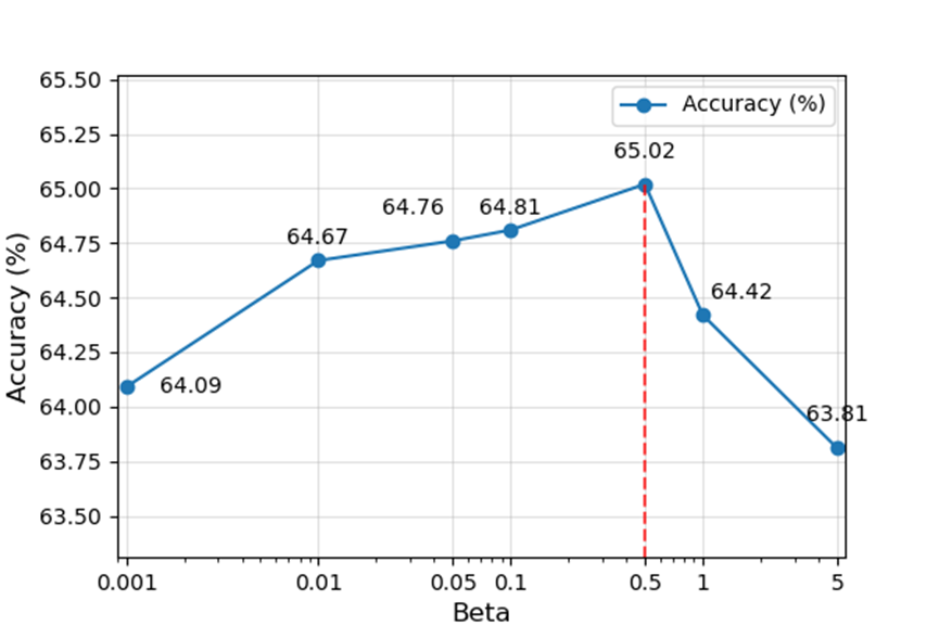
Figure 3: Effect of varying loss function weight $\beta$ on classification accuracy.

To further investigate the impact of traditional image augmentation on the performance of the FAAGC method, we conducted an ablation study. During fine-tuning, we compared two scenarios: (1) without applying image augmentation, a setting consistently applied in all previous experiments; and (2) with image augmentation. The image augmentation techniques used were the default augmentations of the pretrained model, including RandomHorizontalFlip and CenterCrop. The results are summarized in Table 7.

Image Augmentation	FAAGC	Accuracy (%)
No	No	62.14
Yes	No	62.36
No	Yes	64.13
Yes	Yes	64.74

Table 7: Combined Effect of Image Augmentation and FAAGC on Classification Accuracy

Table 7 shows that traditional image augmentation and the FAAGC method operate independently. Applying both methods together leads to further improvements in classification accuracy. This indicates that combining traditional image augmentation with FAAGC is a promising approach for further improving classification performance.

5 Conclusion

We propose a data augmentation technique based on the projected distribution of sample representations in the pre-shape space. The proposed method is simple to implement and demonstrates significant improvements in model performance under data-scarce scenarios. Future work will focus on extending this augmentation method to diverse data modalities and specialized domain-specific datasets, as well as exploring its application to fine-grained downstream tasks. Furthermore, integrating this technique into backbone models has the potential to enhance shape feature extraction during fine-tuning, further improving its effectiveness.

References

- Athalye and Arnaout [2023] Chinmayee Athalye and Rima Arnaout. Domain-guided data augmentation for deep learning on medical imaging. PloS one, 18(3):e0282532, 2023.
- Chu et al. [2020] Peng Chu, Xiao Bian, Shaopeng Liu, and Haibin Ling. Feature space augmentation for long-tailed data. In Computer Vision–ECCV 2020: 16th European Conference, Glasgow, UK, August 23–28, 2020, Proceedings, Part XXIX 16, pages 694–710. Springer, 2020.
- DeVries and Taylor [2017] Terrance DeVries and Graham W Taylor. Dataset augmentation in feature space. arXiv preprint arXiv:1702.05538, 2017.
- Dosovitskiy et al. [2021] Alexey Dosovitskiy, Lucas Beyer, Alexander Kolesnikov, Dirk Weissenborn, Xiaohua Zhai, Thomas Unterthiner, Mostafa Dehghani, Matthias Minderer, Georg Heigold, Sylvain Gelly, Jakob Uszkoreit, and Neil Houlsby. An image is worth 16x16 words: Transformers for image recognition at scale. ICLR, 2021.
- Frid-Adar et al. [2018] Maayan Frid-Adar, Eyal Klang, Michal Amitai, Jacob Goldberger, and Hayit Greenspan. Synthetic data augmentation using gan for improved liver lesion classification. In 2018 IEEE 15th international symposium on biomedical imaging (ISBI 2018), pages 289–293. IEEE, 2018.
- Goodfellow et al. [2014] Ian J Goodfellow, Jonathon Shlens, and Christian Szegedy. Explaining and harnessing adversarial examples. arXiv preprint arXiv:1412.6572, 2014.
- Han et al. [2010] Yuexing Han, Bing Wang, Masanori Idesawa, and Hiroyuki Shimai. Recognition of multiple configurations of objects with limited data. Pattern Recognition, 43(4):1467–1475, 2010.
- Han et al. [2023] Yuexing Han, Guanxin Wan, and Bing Wang. Gcfa: Geodesic curve feature augmentation via shape space theory. arXiv preprint arXiv:2312.03325, 2023.
- Han [2013] Yuexing Han. Recognize objects with three kinds of information in landmarks. Pattern Recognition, 46(11):2860–2873, 2013.
- He et al. [2016] Kaiming He, Xiangyu Zhang, Shaoqing Ren, and Jian Sun. Deep residual learning for image recognition. In Proceedings of the IEEE conference on computer vision and pattern recognition, pages 770–778, 2016.
- Karras et al. [2020] Tero Karras, Miika Aittala, Janne Hellsten, Samuli Laine, Jaakko Lehtinen, and Timo Aila. Training generative adversarial networks with limited data. Advances in neural information processing systems, 33:12104–12114, 2020.
- Kendall et al. [2009] David George Kendall, Dennis Barden, Thomas K Carne, and Huiling Le. Shape and shape theory. John Wiley & Sons, 2009.
- Kendall [1984] David G Kendall. Shape manifolds, procrustean metrics, and complex projective spaces. Bulletin of the London mathematical society, 16(2):81–121, 1984.
- Kingma [2013] Diederik P Kingma. Auto-encoding variational bayes. arXiv preprint arXiv:1312.6114, 2013.
- Krizhevsky et al. [2009] Alex Krizhevsky, Geoffrey Hinton, et al. Learning multiple layers of features from tiny images. 2009.
- Li et al. [2021a] Boyi Li, Felix Wu, Ser-Nam Lim, Serge Belongie, and Kilian Q Weinberger. On feature normalization and data augmentation. In Proceedings of the IEEE/CVF conference on computer vision and pattern recognition, pages 12383–12392, 2021.
- Li et al. [2021b] Pan Li, Da Li, Wei Li, Shaogang Gong, Yanwei Fu, and Timothy M Hospedales. A simple feature augmentation for domain generalization. In Proceedings of the IEEE/CVF International Conference on Computer Vision, pages 8886–8895, 2021.
- Liu et al. [2021] Ze Liu, Yutong Lin, Yue Cao, Han Hu, Yixuan Wei, Zheng Zhang, Stephen Lin, and Baining Guo. Swin transformer: Hierarchical vision transformer using shifted windows. In Proceedings of the IEEE/CVF International Conference on Computer Vision (ICCV), 2021.
- Liu et al. [2024] Dan Liu, Shisheng Zhong, Lin Lin, Minghang Zhao, Xuyun Fu, and Xueyun Liu. Feature-level smote: Augmenting fault samples in learnable feature space for imbalanced fault diagnosis of gas turbines. Expert Systems with Applications, 238:122023, 2024.
- Shorten and Khoshgoftaar [2019] Connor Shorten and Taghi M Khoshgoftaar. A survey on image data augmentation for deep learning. Journal of big data, 6(1):1–48, 2019.
- Tan and Le [2019] Mingxing Tan and Quoc Le. Efficientnet: Rethinking model scaling for convolutional neural networks. In International conference on machine learning, pages 6105–6114. PMLR, 2019.
- Vadgama et al. [2022] Sharvaree Vadgama, Jakub Mikolaj Tomczak, and Erik J Bekkers. Kendall shape-vae: Learning shapes in a generative framework. In NeurIPS 2022 Workshop on Symmetry and Geometry in Neural Representations, 2022.
- Verma et al. [2019] Vikas Verma, Alex Lamb, Christopher Beckham, Amir Najafi, Ioannis Mitliagkas, David Lopez-Paz, and Yoshua Bengio. Manifold mixup: Better representations by interpolating hidden states. In International conference on machine learning, pages 6438–6447. PMLR, 2019.
- Wah et al. [2011] Catherine Wah, Steve Branson, Peter Welinder, Pietro Perona, and Serge Belongie. The caltech-ucsd birds-200-2011 dataset. 2011.
- Wei and Zou [2019] Jason Wei and Kai Zou. Eda: Easy data augmentation techniques for boosting performance on text classification tasks. arXiv preprint arXiv:1901.11196, 2019.
- Xiao [2017] H Xiao. Fashion-mnist: a novel image dataset for benchmarking machine learning algorithms. arXiv preprint arXiv:1708.07747, 2017.