CGAN-Based Framework for Meson Mass and Width Prediction

Generative Adversarial Networks (GANs) are influential machine learning models that have gained prominence across various research fields, including high-energy physics (HEP) simulations. Among them, Conditional GANs (CGANs) offer a unique advantage by conditioning on specific parameters, making them particularly well-suited for meson studies. Given the limited size of the available meson dataset—based on the quark content, quantum numbers, mass, and width—this study, for the first time, applies the CGAN framework to augment the dataset of mesons, while preserving the inherent characteristics of the original data. Using this enhanced dataset, we employ the CGAN model to estimate the mass and width of both ordinary and exotic mesons, based solely on their quark content and quantum numbers. Our CGAN-based predictions highlight the framework’s potential as a reliable tool for meson property estimation, providing valuable insights for future research in particle physics.

1 Introduction

Particle physics investigates the fundamental particles and forces that constitute the building blocks of the universe. Within this broad field, hadron physics focuses specifically on the properties of hadrons, composite particles made of quarks and gluons. The interactions and properties of the hadrons, including mesons and baryons, are crucial to understanding the strong force, as they represent the physical manifestation of quarks and gluons bound together by this force. Quantum Chromodynamics (QCD) is the theoretical framework that describes the interactions between the quarks and gluons, the fundamental constituents of hadrons. QCD explains how the strong force operates at the quark level, dictating their binding within hadrons and giving rise to phenomena like confinement, where quarks are never found in isolation [1, 2, 3, 4, 5, 6, 7, 8, 9].

QCD has been extremely successful in explaining the strong force and the hadronic interactions. Also, its experimental verification is one of the major triumphs of modern physics [8, 9, 10, 11, 12, 13, 14, 15]. However, many aspects of QCD, especially in the non-perturbative regime, continue to be an area of active research [16, 17, 18]. The low-energy behavior of mesons, such as their masses and decay properties, is a window into the non-perturbative aspects of QCD. In experiments, measurements of mesons mass and decay width help to refine our understanding of how quarks and gluons interact when they are bound together to form mesons and other hadrons. So it provides essential input to test theoretical models of QCD in this low-energy regime [19, 20, 21, 22, 23, 24, 25, 26, 27, 28, 29, 30, 31]. Theoretical models in hadron physics are crucial for interpreting experimental results, especially those derived from high-energy collisions at facilities such as the Large Hadron Collider (LHC) [32, 33, 34, 35, 36, 37, 38, 39, 40, 41, 42, 43, 44, 45, 46, 47]. While there has been significant experimental and theoretical progress in the hadron physics, particularly regarding exotic states, the internal structure and quark-gluon configurations of some ordinary and exotic hadrons remain unclear. Additionally, the mass and decay widths of several hadrons, including both ordinary and exotic mesons, have yet to be precisely determined [48, 49, 50, 51, 52, 53, 54, 55, 56]. At this stage, modern simulation techniques have become crucial. As the LHC generates vast amounts of data, simulations are essential tools for unraveling the complexities of hadronic interactions [57, 58, 59, 60, 61, 62, 63, 64, 65]. This dynamic interplay between theory, experiment, and simulation offers a unique opportunity to advance our understanding of hadronic interactions and the complex dynamics of quarks and gluons, particularly in the non-perturbative regime, where traditional analytical methods are less effective in determining the mass and decay widths of hadrons. Traditional methods, such as Monte Carlo simulations, often require significant computational resources and time, especially when dealing with complex systems or high-precision calculations. While advances in technology and new computational techniques, such as machine learning (ML) [66, 67, 68], are helping to alleviate some of these challenges, traditional methods can still be quite demanding. The ML algorithms, particularly those based on deep learning-based generative models, can produce realistic synthetic data that mimics experimental outcomes. This not only enhances the accuracy of simulations but also allows for the exploration of parameter spaces that may not be feasible with traditional methods [69, 70, 71, 72, 73]. By learning patterns from large datasets, ML models can identify relationships between complex variables, optimize simulation parameters, and even predict outcomes that would typically require time-consuming calculations. For example, ML algorithms can be used to accelerate the process of hadronization, predict hadron spectra, or automate the identification of particle decay modes. Additionally, ML can be employed to analyze and interpret experimental data more effectively, allowing for faster and more precise extraction of physical quantities such as cross-sections, particle trajectories, and event classification. These advancements are helping to bridge the gap between traditional simulation methods and the vast amounts of data generated by modern high-energy physics experiments, making it possible to explore new regions of parameter space and extract insights more efficiently [74, 75, 76, 77, 78, 79, 80, 81, 82, 83, 84]. This collaboration between the simulation and the ML is paving the way for deeper insights into the hadron physics. More accurate event classification, improving parameter estimation, and facilitating the development of sophisticated simulations in hadronic data are advanced techniques that enrich our understanding of the hadron physics [77, 78, 85, 86, 87, 88, 89]. Deep learning-based generative models are able to generate new data samples from learned distributions. They have gained significant attention due to their ability to produce high quality outputs [73, 90, 91, 92, 93]. Common methods for deep generative models include variational autoencoders (VAEs) [94, 95], normalizing flows (Nfs) [96, 97], and generative adversarial networks (GANs) [74, 98, 99]. For instance, the VAE framework has been introduced to generate realistic and diverse HEP events. This model benefits from several techniques in the VAE literature to simulate high-fidelity jet images [94]. Normalizing flows is one of the approaches employed to directly generate full events at the detector level from Parton-level information. As such, this research represents an important step in advancing generative modeling techniques in high-energy physics [97]. GANs are a class of deep learning generative models where two neural networks, a generator, and a discriminator, compete against each other to produce realistic synthetic data. The generator creates new data samples, while the discriminator evaluates them against real data, guiding the generator to improve its output [98]. In recent years, GANs have become influential techniques in a variety of scientific fields, including particle physics. GANs have been effectively used to generate high-fidelity event samples in collider physics, enabling the production of complex multi-particle final states that closely resemble actual collision data. This application helps in simulating and analyzing particle interactions more efficiently [74, 90, 99, 100, 101, 102]. The hadronization plays a crucial role in simulating high-energy experiments. Ref. [90], has introduced a protocol for training a deep generative model for hadronization, employing a GAN framework with a permutation-invariant discriminator. The authors assert that their work marks a significant advancement in the ongoing effort to develop, train, and incorporate the ML-based models of hadronization into parton shower Monte Carlo simulations. A specialized variant of GANs, known as Conditional GANs (CGANs), modify the GAN setup by conditioning both the generator and the discriminator on additional information. This could be labels, images, or any other type of data that specifies a desired output, helping generate more targeted data [103]. In the hadron physics, CGANs can be used for the event generation, the simulation of HEP collisions, the parameter estimation and identifying anomalies in new data, such as potential signals of new physics [101, 104]. A recent study has shifted its focus from traditional full-simulation methods to investigate the potential of a deep learning-based CGAN. The research presents a fast simulation technique that uses CGANs to convert calorimeter images, offering the potential to significantly reduce both computational time and disk space requirements for the LHC and future high-energy physics experiments [101]. The generative models, due to their ability to create synthetic data, have become increasingly valuable in the field of generative data augmentation [100, 105]. The data augmentation techniques are commonly employed when the available data for analysis or simulation is limited, as this limitation can lead to reduced model accuracy and generalization. By artificially increasing the diversity of the training data, data augmentation helps improve the robustness of models, especially in fields like ML and HEP, where acquiring large amounts of labeled data can be costly or time-consuming. Despite significant achievements in the HEP, including the cataloging of numerous mesonic and baryonic states by the PDG [4, 5], the available dataset for studying these states through the deep generative models remains limited. In this context, data augmentation techniques can provide a useful solution [100, 105, 106, 107]. It should be noted that two methods have been presented to augment the available hadronic data so far. In the first method, experimental mass errors are added to and subtracted from their central values, while the quantum numbers remain fixed. This results in the training data being resampled twice. The second method employs Gaussian noise resampling, using a Gaussian probability density function. In this approach, random data points are generated based on the mean values and errors from the training dataset, with the quantum numbers of the hadrons held constant. The hadronic data undergoes up to 9 data replications using this method [84, 108]. Building on this foundation, we have developed, for the first time, a CGAN model specifically designed to augment existing meson data. By harnessing the power of CGANs, we generate synthetic meson data that closely mirrors the distribution and characteristics of real-world measurements. This approach has the potential to advance data-driven studies in hadron physics, providing a more comprehensive dataset for further analysis, model training, and improved predictions of mesonic properties. One key controversy in the field involves the quark content of certain mesons, with ongoing ambiguity about whether they should be classified as ordinary mesons or exotic states, such as tetraquarks. Additionally, the masses and decay widths of both ordinary and exotic mesons remain poorly measured, contributing to the uncertainties and debates within hadron physics. Notably, the fundamental properties of the meson spectrum have been used to estimate the masses of baryons, pentaquarks, and other exotic hadrons [83]. Inspired by this framework, we developed deep neural networks (DNNs) to more accurately estimate the mass and decay width of both ordinary and exotic mesons [79]. In this study, we utilize CGANs not only to augment the mesonic dataset but also to enhance the accuracy of mass and decay width estimates for controversial mesons, whose properties remain uncertain. By using the CGANs, we aim to improve the predictive power and reliability of these estimations, thereby contributing to a deeper understanding of both ordinary and exotic mesons.

2 Generative Adversarial Networks

Neural networks (NNs) are computational models based on the architecture and processes of the human brain. They are designed to identify patterns and relationships within data through a network of interconnected layers. Each layer comprises artificial neurons, which perform fundamental computations to process and transform information:

• Input Layer: This layer takes in raw data features and transmits them to the subsequent layers, with the number of neurons matching the number of input features.

• Hidden Layers: These layers process inputs using weights and biases, applying activation functions to capture non-linear relationships. The number and size of hidden layers determine the model’s capacity.

• Output Layer: This layer generates the model’s final predictions, translating the processed information from the hidden layers into a usable result. The number of neurons here corresponds to the number of outputs required (e.g., for a classification task, it could be the number of classes).

Each neuron computes a weighted sum of its inputs, adds a bias term, and applies an activation function, as described by the following equation:

$$\text{Output}=f\left(\sum_{i=1}^{n}w_{i}x_{i}+b\right),$$ (1)

where $x_{i}$ are the inputs, $w_{i}$ are the weights, $b$ is the bias, and $f$ is the activation function.

Common activation functions include:

• Sigmoid: $f(x)=\frac{1}{1+e^{-x}}$, maps inputs to a range between 0 and 1.

• ReLU (Rectified Linear Unit): $f(x)=\max(0,x)$, introduces sparsity and mitigates the vanishing gradient problem.

• Tanh: $f(x)=\tanh(x)$, maps inputs to a range between -1 and 1.

The training process involves minimizing a loss function, which quantifies the difference between predicted and actual outputs. This is achieved using optimization algorithms such as gradient descent, which iteratively adjusts the weights and biases to reduce the loss. The update rule is:

$$\theta\rightarrow\theta-\eta\frac{\partial\mathcal{L}}{\partial\theta},$$ (2)

where $\theta$ represents the model parameters (weights and biases), $\eta$ is the learning rate, and $\mathcal{L}$ is the loss function.

Backpropagation efficiently computes gradients by propagating errors from the output layer back through the earlier layers. This process ensures that each layer adjusts to minimize its contribution to the overall error.

NNs, with their layered architecture, activation functions, and loss functions, have revolutionized numerous domains by learning complex patterns from data. However, traditional NNs are primarily designed for predictive tasks, such as classification or regression, which involve mapping inputs to outputs. To address the challenge of data generation and expand the capabilities of NNs, researchers have introduced advanced architectures like GANs. GANs build on the foundational principles of NNs but take them further by incorporating two competing networks -generator and discriminator- that work together to create data indistinguishable from the real dataset.

GANs are a class of ML frameworks introduced by Ian Goodfellow and his colleagues in 2014 [98]. GANs comprise two NNs, a generator ($G$) and a discriminator ($D$), which are trained simultaneously through adversarial learning. The generator aims to create realistic data samples, while the discriminator’s task is to differentiate between real and generated data. The adversarial nature of this process enables GANs to generate synthetic data that closely corresponds to real data.

The training process of GANs is formulated as a min-max optimization problem, where the generator and discriminator engage in a two-player game. The objective function is given by:

$$\min_{G}\max_{D}\mathcal{L}(D,G)=\mathbb{E}_{x\sim p_{\text{data}}(x)}[\log D(x)]+\mathbb{E}_{z\sim p_{z}(z)}[\log(1-D(G(z)))],$$ (3)

where $p_{\text{data}}(x)$ represents the distribution of real data, $p_{z}(z)$ is the prior distribution of the input noise $z$, $G(z)$ generates fake data, and $D(x)$ outputs the probability that $x$ is real.

The adversarial learning framework ensures that the generator improves over time by "fooling" the discriminator, while the discriminator simultaneously becomes more proficient at distinguishing real data from generated data. This adversarial process continues until the generator produces data that the discriminator can no longer consistently differentiate from real data.

Despite their success, GANs face several challenges, including mode collapse, where the generator produces a limited range of outputs, and training instability arising from the min-max optimization process. Various techniques have been proposed to address these issues, such as Wasserstein GAN (WGAN) and gradient penalty, which enhance training stability by modifying the loss function.

CGANs build upon the GAN framework by integrating extra information, such as class labels $y$ or specific features, into the data generation process. In CGANs, the generator and discriminator both rely on conditioning with $y$, and the objective function is modified accordingly

$$\min_{G}\max_{D}\mathcal{L}(D,G)=\mathbb{E}_{x,y\sim p_{\text{data}}(x,y)}[\log D(x|y)]+\mathbb{E}_{z\sim p_{z}(z),y\sim p_{y}(y)}[\log(1-D(G(z|y)|y))].$$ (4)

This conditioning enables CGANs to generate data that is not only realistic but also conforms to specified characteristics. In the context of regression tasks, $y$ can represent numerical values, prediction bounds, or parameters that directly influence the generated data. For example, if the goal is to predict the mass of a particle, $y$ could include quantum features of the particle such as spin, charge, or isospin, ensuring that the generated data remains consistent with these attributes.

The primary advantage of CGANs in particle physics is their ability to incorporate domain-specific constraints, ensuring that generated data adheres to the physical laws and characteristics of the problem. GANs and CGANs have become important tools in the field of particle physics, enabling researchers to simulate and analyze complex phenomena.

Some notable applications include:

• Data Augmentation: GANs can be employed to generate synthetic datasets for rare events in HEP experiments, such as collisions in particle accelerators.

• Detector Simulation: GANs can assist in simulating particle trajectories in detectors, reducing computational costs compared to traditional Monte Carlo methods.

• Quantum System Simulation: GANs are capable of aiding in modeling quantum systems by generating data consistent with experimental results.

• Hadronic Properties: In this study, CGAN frameworks were employed to enhance the limited data on mesons and to predict their masses and decay widths by conditioning on quantum properties.

The section 3 provides a detailed explanation of data augmentation using CGANs. It is worth mentioning that we applied the bagging technique to the CGAN model to aggregate predictions from multiple instances, thereby quantifying uncertainty in the generated outputs and improving the overall stability of the predictions. In this method, we set up $N$ independent CGANs: $\text{CGAN}_{1},\text{CGAN}_{2},\dots,\text{CGAN}_{N}$, with $N$ being the number of models. Random sampling from the training data generates subsets, $\text{training data}_{1},\text{training data}_{2},\dots,\text{training data}_{N}$, which are used to train each CGAN model. This process, called bootstrapping, allows each model to learn different representations of the data. After training, each CGAN produces predictions, denoted as $P_{1},P_{2},\dots,P_{N}$. The final output is obtained by averaging these predictions, $\hat{P}=<\hat{P_{i}}>\equiv N^{-1}\Sigma_{i}\hat{P_{i}}$. The variance across the predictions provides a measure of uncertainty, with higher variability indicating greater uncertainty in the model’s output. This entire process, including bootstrapping and aggregation, is referred to as bagging [109]. In this work, we choose $N=10$ CGAN models. The bagging technique is known to reduce the variance of the model predictions, which helps to reduce overfitting by averaging out fluctuations in the individual models’ outputs. This leads to more stable and reliable predictions, especially in the presence of noisy data. The final output $\hat{P}$ is less prone to extreme predictions compared to a single model. The approach is well illustrated in Fig. 1.

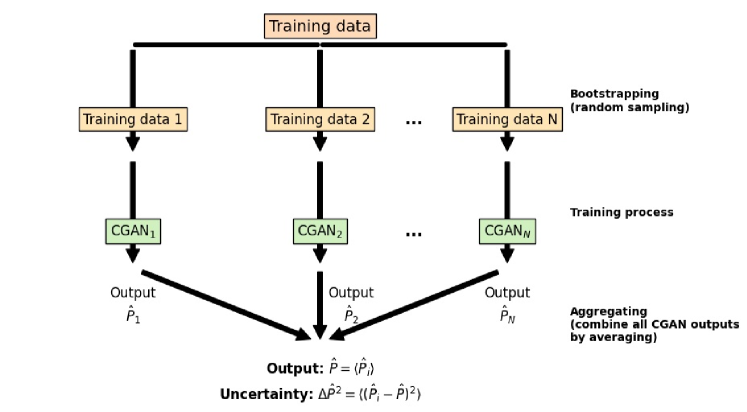
Figure 1: Illustration of the bagging technique applied to the CGAN model. The method involves training $N$ independent CGAN models on different subsets of the training data, which are created through random sampling (bootstrapping).

3 Data augmentation and preprocessing

As the NNs grow in complexity and scale, training leading-edge models requires vast amounts of data. However, producing such data is often both resource-intensive and time-consuming. To manage this, one can either enhance the existing dataset with additional descriptive variables or mitigate data scarcity by artificially expanding the dataset through creation of new instances, bypassing the need for resource-intensive data generation. These approaches are collectively referred to as data augmentation techniques in ML applications. The first category of these methods, often called feature generation or feature engineering, is applied at the instance level. It involves creating new input features to provide more meaningful data for the algorithm, enhancing its ability to learn effectively. The second category of methods operates at the dataset level and can generally be divided into two main approaches. The first approach is known as real data augmentation, which involves making slight modifications to real data to create new samples. For instance, techniques like rotation or zooming are commonly used to augment image datasets. The second approach is synthetic data augmentation, where new data is generated entirely from scratch. This includes traditional sampling techniques and advanced generative models, such as GANs, which are capable of producing highly realistic synthetic datasets. Thus, by generating the synthetic data samples that retain key features or distributions of the original data, the synthetic data augmentation helps improve model generalization, enhances predictive performance, and facilitates the discovery of meaningful patterns in both experimental and simulated datasets. In particle physics, the collection of experimental data is often both time-intensive, laborious and costly. Large-scale experiments, such as those conducted with particle colliders (e.g., the LHC), produce enormous volumes of data that require extensive preprocessing, analysis, and refinement to uncover meaningful insights. In LHC experiments, the data augmentation approach are introduced to accelerate simulation workflows. This method employs a generative deep learning model to transform collision events from an analysis-specific generator-level representation into their corresponding reconstruction-level representation [110]. Ref. [109] augmented the training data using noise fluctuations corresponding to observational uncertainties. They suggest that the data augmentation could be an effective technique for reducing the possibility of overfitting without the need to adjust the NN architecture, such as by inserting dropout. Applying deep learning methods to hadron physics may present several challenging problems. While PDG [4, 5] has cataloged hundreds of mesonic and baryonic states, the relatively limited number of known hadrons can pose significant challenges for advanced deep learning models. This scarcity of data may hinder the training process, potentially affecting the model’s ability to generalize and make accurate predictions, especially when addressing complex phenomena in hadron physics. Two methods have been introduced for augmenting the hadronic data so far. The first involves adding and subtracting experimental mass errors from their central values while keeping the quantum numbers of hadrons fixed, effectively resampling the training data twice. The second method utilizes Gaussian noise resampling, generating random data points based on a Gaussian probability density function derived from the dataset’s mean values and errors. This approach allows for up to nine replications of the hadronic data, with quantum numbers remaining constant throughout [84, 108]. Generative models, such as CGANs, present a powerful option for data augmentation in particle physics, particularly for generating synthetic hadronic data. A CGAN framework accomplishes this by producing synthetic samples conditioned on specific parameters or features, ensuring that the generated data adheres to the desired properties and aligns with the underlying physical characteristics. In this study, we focus on mesons, both ordinary and exotic, whose quark compositions and quantum numbers, including isospin ($I$), angular momentum ($J$), parity ($P$), $G$-parity, and $C$-parity, have been determined and confirmed by PDG [4, 5]. It should be noted that mesons with identical quark structures and quantum numbers but differing masses can create ambiguity in data analysis. To handle this, an additional feature referred to as the higher state ($h$) is introduced. It is important to emphasize that $h$ is not a real quantum number. As outlined in our recent study [79], $h$ serves solely to differentiate particles with similar properties but varying masses. For instance, $\rho(770)$ and $\rho(1450)$ share identical input features but differ in the mass. Thus, they are assigned $h$ values of $0$ and $1$, respectively, allowing them to be recognized as distinct entities by ML algorithms. The range of $h$ can vary from $0$ to $10$, depending on the number of similar mesons. Ultimately, this results in the vector below as an input,

$$\vec{v}=(d,\bar{d},u,\bar{u},s,\bar{s},c,\bar{c},b,\bar{b},I,J,P,h,G,C).$$ (5)

We have adopted the conventions recommended in Ref. [83] and our recent study [79] to specify the valence quarks of mesons known with linear combination of quark-antiquark pairs. For example, the feature values of valence quarks of isotriplet mesons like $\pi_{0}$ and $\rho_{0}$ are $(1,1,\vec{0}_{8},I,J,P,h,G,C)$. The values of $G$ or $C$ parameters are set to zero for mesons that are not eigenstates of G-parity or C-parity. We categorized these mesons into two distinct datasets. the training dataset, comprising the mesons with accurately measured masses, and the test dataset, consisting of the mesons whose masses have yet to be determined. Furthermore, we extended this categorization considering the decay width of the mesons. In a similar manner, the mesons with all features—including quark compositions, quantum numbers, $h$, mass and decay width—fully determined, were classified into the training dataset. Conversely, the mesons with unclear or undetermined decay width values were assigned to the test dataset. This approach ensures a robust division of data, enabling focused training on well-characterized mesons while reserving those with incomplete information for testing and evaluation. It is necessary to mention that, the mass and decay width of the mesons are expressed in units of MeV. However, number of the mesons in our training dataset is limited, necessitating expansion to support high-level deep learning architectures. To manage this, we looked for an effective and professional approach to generate synthetic mesonic samples. The CGAN framework proved instrumental in achieving this goal, producing meaningful and reliable augmented data. For this purpose, CGAN takes the training data along with the associated experimental uncertainties in the mass or decay width. It is conditioned on features such as the quark content and quantum numbers ($I$, $J$, $P$, $C$, $G$) that remain constant, allowing only the mass or width parameters to vary within their experimental range during the augmentation process. Consequently, we obtained synthetic training data that preserves the key properties of mesons, generated using one of the most effective generative models. The mesonic dataset was expanded by a factor of five, significantly increasing its size to enhance model training and analysis. Fig. 2, shows a side-by-side comparison of the heatmaps for the original and augmented meson datasets, providing strong evidence that the augmented data preserves the patterns and distributions of the original dataset. This comparison highlights the effectiveness of our CGAN framework in augmenting meson data and demonstrates the reliability of the augmentation method.

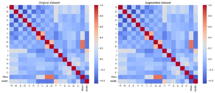
Figure 2: Side-by-side comparison of heatmaps for the original and augmented meson datasets, demonstrating how the augmented data preserves the patterns and distributions of the original dataset.

Following the data augmentation process, the next step involves scaling the mass and decay width values in the dataset. This is achieved using standard scaling techniques commonly employed in data science, such as normalization or standardization, to ensure that these values fall within a constrained range. Scaling not only aids in stabilizing the training process but also helps improve the model’s ability to learn effectively from the data. Since the mass and width parameters are dimensionful, they are divided by 1 MeV to make them dimensionless before applying scaling. With this step completed, the dataset preparation process is finalized. At this stage, the input data is fully prepared and ready to be fed into our CGAN model to initiate the training process.

4 Discussion

In this part we give and explain our numerical results obtained using our CGAN model. We aim to predict the masses of several well-known, light mesons and exotic mesons, as well as the decay widths of mesons whose values have not yet been experimentally determined. The numerical results for the predicted masses and decay widths, along with the corresponding mean errors, are presented in Tables 1 to 6 The uncertainty in the predicted results has been determined using the bagging method described in Sec. 2.

4.1 Ordinary or exotic mesons: an ongoing debate

In contrast to ordinary mesons, tetraquarks are considered exotic mesons that fall outside the traditional framework of the quark model. While ordinary mesons consist of a single quark-antiquark pair, tetraquarks contain four valence quarks, two quarks and two antiquarks, leading to their classification as more complex hadrons. Despite their unconventional structure, tetraquarks are still categorized as mesons because they consist of an equal number of quarks and antiquarks, adhering to the basic definition of mesons. Although the quark model was first introduced by Gell-Mann in 1964 [1], he also proposed the possibility of more exotic hadrons, beyond the conventional quark-antiquark structure of mesons and the three-quark structure of baryons. Since then, many mesons both ordinary and exotic have been discovered, yet the quark content of some remains ambiguous. This uncertainty raises the question of whether certain mesons should be classified as conventional ($q\bar{q}$) mesons or whether they may represent a new class of exotic hadrons, such as tetraquarks. In this study, we aim to predict the mass of several challenging mesons, including $a_{0}(980)$, $f_{0}(980)$, $D_{s0}^{*}(2317)^{\pm}$ and $D_{s1}(2460)^{\pm}$ using our CGAN model based on two key assumptions. first, we consider the $q\bar{q}$ structure, and then explore possibility of the $q\bar{q}q\bar{q}$ structure for their quark contents. Table 1 illustrates the numerical results compared to the experimental [111], as well as our previous DNN results[79]. According to the Table 1, our CGAN prediction for the mass of $a_{0}(980)$ in the $u\bar{u}$ configuration yields $983\pm 44\,~\text{MeV}$, which is significantly closer to the experimental value of $980\pm 20\,\text{MeV}$ than our previous DNN result of $998\pm 94\,~\text{MeV}$. Such notable prdiction is also obtained when the $u\bar{s}\bar{u}s$ configuration is supposed for $a_{0}(980)$. In fact, the masses estimated by the CGAN are not only closer to the experimental values but also exhibit smaller uncertainty ranges compared to the DNN results. If we examine the other particles in Table 1, we find that our CGAN predictions outperform the DNN results for both ordinary and exotic assumptions. Besides our CGAN model results suggest that, based on the predicted mass distributions, the possibility of these mesons being tetraquarks cannot be ruled out.

4.2 Light mesons

The mass of $f_{0}(500)$ is known to lie within the range of $400$ to $800$ MeV (see Table 2). Our CGAN prediction yields a mass of $547\pm 102\,~\text{MeV}$, which falls well within this range. In comparison, the DNN model estimates the mass to be $759\pm 134\,~\text{MeV}$, which is closer to the upper end of the known range. While both predictions are within the experimentally expected range, the CGAN prediction provides a value closer to the central region of the mass range. The smaller uncertainty range in the CGAN prediction also suggests a more confident estimation compared to the DNN result. Our CGAN predictions for the masses of $K_{4}(2500)_{0},\bar{K_{4}}(2500)_{0}$ and $K_{4}^{\pm}(2500)$ are in good agreement with the experimental values. Our CGAN predictions for the mass of $K_{2}(1580)_{0},\bar{K_{2}}(1580)_{0}$ is $1702\pm{93}$ and for the mass of $K_{2}^{\pm}(1580)$ is $1733\pm{98}~\text{MeV}$, which are somewhat higher than the experimental value. Despite this discrepancy, the CGAN predictions provide valuable insight into the mass range, though further refinement may be needed for more accurate alignment with the experimental mass.

4.3 Exotic mesons

In this section, we present our CGAN predictions for the mass of several exotic states comparing them to experimental measurements as well as the results obtained from our previous DNN model (see Table 3). The CGAN model predicts a mass of $3716\pm{140}~\text{MeV}$ for $\chi_{c1}(3872)$. While this prediction is not an exact match to the experimental value of $3871.65\pm{0.06}~\text{MeV}$, it is still much closer than the DNN prediction of $2944\pm{177}~\text{MeV}$, highlighting the superior accuracy of the CGAN model in this instance. For states such as $\psi(4230)$, $\psi(4360)$ and $\psi(4660)$, our CGAN model yields predictions that are notably closer to the experimental values than the DNN predictions. Also, the CGAN strongly predicts the mass of $Z_{c}(3900)^{\pm}$ state, where the experimental mass is reported as $3887.1\pm{2.6}~\text{MeV}$, The CGAN prediction of $3876\pm{210}~\text{MeV}$, is very close to this value, demonstrating its ability to accurately capture the mass of this state. While there is some uncertainty in the CGAN prediction, it is still within a reasonable range of the experimental measurement. This trend persists for other exotic states listed in the table. For instance, the CGAN estimates the mass of $Z_{b}(10650)^{\pm}$ to be $10675\pm{691}~\text{MeV}$, which aligns closely with the experimental value of $10652.2\pm{1.5}~\text{MeV}$.

These comparisons highlight the advanced performance of the CGAN model, especially when combined with the augmentation technique, compared to our previous DNN model. The augmentation of the training data plays a critical role in enhancing the model’s ability to learn complex patterns and generalize more effectively. By artificially expanding the dataset, we provide the model with a more diverse set of examples. This enriched data allows the CGAN model to better capture the underlying relationships between features, resulting in more accurate and robust predictions. Furthermore, the augmentation technique also contributes to reducing overfitting, which is often a challenge in deep learning models with limited data. By exposing the CGAN to a broader range of training examples, we improve its ability to handle unseen data with greater precision, particularly for the challenging task of predicting the masses and width of exotic states. Thus, the CGAN model, with the added benefit of data augmentation, outperforms the DNN not only in terms of prediction accuracy but also in its ability to generalize and handle complex patterns with higher precision.

Meson	$I^{G}\,(J^{PC})$	Exp. Mass (MeV) [111]	quark content	DNN[79]	CGAN model
$a_{0}(980)$	$1^{-}\,(0^{++})$	$980\pm 20$	$u\bar{u}$	$998\pm{94}$	$983\pm{44}$
			$u\bar{s}\bar{u}s$ $(K\overline{K})$	$1069\pm{224}$	$994\pm{142}$
$f_{0}(980)$	$0^{+}\,(0^{++})$	$990\pm 20$	$d\bar{d}$	$883\pm{45}$	$805\pm{60}$
			$d\bar{s}\bar{d}s$ $(K\overline{K})$	$1086\pm{68}$	$1032\pm{27}$
$D_{s0}^{*}(2317)^{\pm}$	$0\,(0^{+})$	$2317.8\pm 0.5$	$\pm{}$ $c\bar{s}$	$2343\pm{169}$	$2312\pm{49}$
			$c\bar{u}u\bar{s}$ $(DK)$	$2511\pm{334}$	$2344\pm{70}$
$D_{s1}(2460)^{\pm}$	$0\,(1^{+})$	$2459.5\pm 0.6$	$c\bar{s}$	$2442\pm{218}$	$2447\pm{48}$
			$c\bar{u}u\bar{s}$ $(D^{*}K)$	$2748\pm{504}$	$2365\pm{132}$

Table 1: Predictions of our CGAN model for the masses of four well-known conventional mesons compared to their corresponding tetraquark structures (in MeV). Results are presented alongside experimental data [111] and our previous DNN model predictions in Ref. [79].

Meson	$I^{G}\,(J^{PC})$	Exp. Mass (MeV) [111]	quark content	DNN[79]	CGAN model
$f_{0}(500)$	$0^{+}\,(0^{++})$	$400-800$	$d\bar{d}$	$759\pm{134}$	$547\pm{102}$
$K_{4}(2500)_{0},\bar{K_{4}}(2500)_{0}$	$1/2\,(4^{-})$	$2490\pm{20}$	$d\bar{s},s\bar{d}$	$2308\pm{35}$	$2397\pm{55}$
$K_{4}^{\pm}(2500)$	$1/2\,(4^{-})$	$2490\pm{20}$	$u\bar{s},s\bar{u}$	$2298\pm{25}$	$2404\pm{89}$
$K_{2}(1580)_{0},\bar{K_{2}}(1580)_{0}$	$1/2\,(2^{-})$	$1580$	$d\bar{s},s\bar{d}$	$1646\pm{20}$	$1702\pm{93}$
$K_{2}^{\pm}(1580)$	$1/2\,(2^{-})$	$1580$	$u\bar{s}$	$1653\pm{23}$	$1733\pm{98}$

Table 2: Predictions of our CGAN model for the mass of some light mesons (in units of MeV). Results are presented alongside experimental data [111] and our previous DNN model predictions in Ref. [79].

Meson	$I^{G}\,(J^{PC})$	Exp. Mass (MeV) [111]	quark content	DNN[79]	CGAN model
$\chi_{c1}(3872)$	$0^{+}\,(1^{++})$	$3871.65\pm 0.06$	$c\bar{u}\bar{c}u$ $(D^{0}\,\bar{D}^{*0})$	$2944\pm{177}$	$3716\pm{140}$
$\psi(4230)$	$0^{-}\,(1^{--})$	$4222.5\pm 2.4$	$c\bar{s}\bar{c}s$ $(D_{s}\,\bar{D}_{s})$	$3303\pm{175}$	$4076\pm{190}$
$\psi(4360)$	$0^{-}\,(1^{--})$	$4374\pm 7$	$c\bar{u}\bar{c}u$ $(D_{1}\,\bar{D}^{*})$	$3190\pm{184}$	$4204\pm{175}$
$\psi(4660)$	$0^{-}\,(1^{--})$	$4630\pm 6$	$c\bar{u}\bar{c}u$ $(f_{0}(980)\,\psi^{\prime})$	$3300\pm{79}$	$4456\pm{251}$
$Z_{c}(3900)^{\pm}$	$1^{+}\,(1^{+-})$	$3887.1\pm 2.6$	$\bar{c}uc\bar{d}$ $(D\,\bar{D}^{*})$	$3676\pm{183}$	$3876\pm{210}$
$Z_{c}(4200)^{\pm}$	$1^{+}\,(1^{+-})$	$4196^{+35}_{-32}$	$\bar{c}uc\bar{d}$	$3981\pm{195}$	$4172\pm{103}$
$Z_{c}(4430)^{\pm}$	$1^{+}\,(1^{+-})$	$4478^{+15}_{-18}$	$\bar{c}uc\bar{d}$ $(D_{1}D^{*}\,,\,D_{1}^{\prime}D^{*})$	$4052\pm{197}$	$4011\pm{676}$
$Z_{b}(10610)^{\pm}$	$1^{+}\,(1^{+-})$	$10607.2\pm 2.0$	$b\bar{d}\bar{b}u$ $(B\bar{B}^{*})$	$8918\pm{447}$	$10486\pm{685}$
$Z_{b}(10650)^{\pm}$	$1^{+}\,(1^{+-})$	$10652.2\pm 1.5$	$b\bar{d}\bar{b}u$ $(B^{*}\bar{B}^{*})$	$9103\pm{159}$	$10675\pm{691}$
$Z_{cs}(4220)^{+}$	$1/2\,(1^{+})$	$4216^{+50}_{-40}$	$u\bar{c}\bar{s}c$	$3054\pm{182}$	$4144\pm{138}$
$R_{c0}(4240)$	$1^{+}\,(0^{--})$	$4239^{+50}_{-21}$	$c\bar{u}\bar{c}u$	$3760\pm{469}$	$4096\pm{102}$

Table 3: Predictions of our CGAN model for the mass of some exotic mesons (in units of MeV). Results are presented alongside experimental data [111] and our previous DNN model predictions in Ref. [79].

4.4 Fully heavy tetraquarks

The experiments at the LHC, conducted by collaborations such as LHCb, ATLAS, and CMS, have played a transformative role in advancing our understanding of exotic hadronic states. Recently, resonances such as $X(6200)$, $X(6600)$, $X(6900)$, and $X(7300)$ have been observed in the invariant mass spectra of di-$J/\psi$ and $J/\psi\psi^{\prime}$. These discoveries have enhanced both theoretical and experimental efforts to explore fully-heavy tetraquark systems composed of $c$- and $b$-quarks [112, 113, 114].

Fully-heavy tetraquarks, characterized by their unique structure consisting only of heavy quarks and antiquarks (e.g., $cc\bar{c}\bar{c}$ or $bb\bar{b}\bar{b}$), represent a distinct class of multiquark states. Unlike conventional mesons and baryons, these exotic states open up a new perspective on the dynamic of QCD in the non-perturbative regime. Their existence was theorized decades ago, tracing back to the pioneering work of Gell-Mann and Zweig during the development of the quark model [115, 116]. Theoretical predictions for these states first emerged from non-relativistic potential models, QCD sum rules, and lattice QCD calculations [117, 118, 119].

The LHCb collaboration’s landmark observation of structures in the di-$J/\psi$ spectrum provided the first compelling evidence for fully-charmed tetraquark candidates. These resonances were identified with masses that significantly exceed the thresholds of conventional charmonium states, These findings confirmed their exotic nature, with subsequent analyses by the ATLAS and CMS collaborations providing high-statistics data that helped constrain their properties, including masses and decay widths. [114].

These experimental achievements have paved the way for future searches, including investigations into fully-bottom ($bb\bar{b}\bar{b}$) and mixed heavy-quark configurations (e.g., $bc\bar{b}\bar{c}$). The upcoming high-luminosity LHC (HL-LHC) and Belle II experiments are expected to increase sensitivity to these states, potentially revealing new tetraquark families.

The theoretical understanding of fully-heavy tetraquarks has evolved significantly [120, 121, 122, 123, 124, 125, 126, 127, 128, 129, 130, 131]. Early studies used diquark-antidiquark configurations to estimate masses and binding energies of these states. Using QCD sum rules, studies have systematically explored quantum numbers such as $J^{PC}=0^{++},1^{++},$ and $2^{++}$. These analyses consistently predict masses above the dissociation thresholds of two quarkonium states, indicating their dominant decay modes [132, 133, 134, 135].

Despite significant progress, several open questions remain. For instance, the stability of fully-heavy tetraquarks against strong decays has yet to be comprehensively understood. Additionally, the role of chromoelectric and chromomagnetic interactions in binding these systems is still debated. Recent studies using QCD sum rules and lattice QCD have shown promise in improving mass estimates and exploring decay channels. In contrast, we employed the CGAN framework to predict the masses of some of these tetraquarks, further enhancing our understanding of their properties. Table 4 presents CGAN-based predictions for fully-heavy tetraquark masses. It should be noted that, $T_{cc\bar{c}\bar{c}}$, the only heavy tetraquark in Table 4 with an experimentally measured mass, serves as a benchmark for comparison. The experimentally measured mass is reported as $6899\pm 12~\text{MeV}$. Our CGAN estimate for this heavy tetraqurk is $6763\pm{681}~\text{MeV}$. While it seems a difference between the experimental and predicted values, this prediction was particularly challenging due to the complex nature of fully heavy tetraquarks. Nonetheless, the predicted result demonstrates the potential of our CGAN framework in making non-trivial mass prediction, and further refinements could bring the estimate closer to experimental value. The remaining CGAN predictions for heavy tetraquarks in Table 4 are presented alongside theoretical estimates for comparison.

Meson	$I^{G}\,(J^{PC})$	Mass (MeV)	CGAN model
$T_{cc\bar{c}\bar{c}}$	$0^{+}\,(0^{++})$	$6899\pm 12$ [111](Exp. Mass)	$6763\pm{681}$
$T_{cc\bar{c}\bar{c}}^{*}$	$0^{+}\,(0^{++})$	$7235\pm 75$ [122]	$7014\pm{371}$
$T_{bb\bar{b}\bar{b}}$	$0^{+}\,(0^{++})$	$18858\pm{50}$ [120]	$18388\pm{912}$
$T_{bb\bar{b}\bar{b}}^{*}$	$0^{+}\,(0^{++})$	$18540\pm{50}$ [123]	$19100\pm{965}$
$T_{cc\bar{c}\bar{b}}$	$0^{+}\,(0^{+})$	$9680\pm 102$[131]	$9736\pm{681}$
$T_{bb\bar{b}\bar{c}}$	$0^{+}\,(0^{+})$	$15697\pm{95}$[131]	$15006\pm{857}$
$T_{bb\bar{c}\bar{c}}$	$0^{+}\,(0^{+})$	$12715\pm{86}$ [124]	$13054\pm{917}$
$T_{bb\bar{c}\bar{c}}$	$0^{+}\,(0^{-})$	$13092\pm{950}$ [127]	$12774\pm{821}$
$T_{bb\bar{c}\bar{c}}$	$0^{+}\,(1^{-})$	$13092\pm{95}$ [127]	$11312\pm{980}$
$T_{bb\bar{c}\bar{c}}$	$0^{+}\,(2^{+})$	$12795\pm{950}$ [126]	$11908\pm{726}$
$T_{bc\bar{b}\bar{c}}$	$0^{+}\,(0^{++})$	$12697\pm{90}$ [128]	$11880\pm{592}$
$T_{bc\bar{b}\bar{c}}$	$0^{+}\,(0^{-+})$	$----$	$11806\pm{680}$
$T_{bc\bar{b}\bar{c}}$	$0^{+}\,(1^{-+})$	$----$	$11699\pm{506}$
$T_{bc\bar{b}\bar{c}}$	$0^{+}\,(1^{++})$	$12715\pm{90}$ [129]	$11783\pm{940}$
$T_{bc\bar{b}\bar{c}}$	$0^{+}\,(2^{++})$	$12700\pm{90}$ [130]	$11470\pm{303}$

Table 4: Predictions of our CGAN model for the mass of fully heavy tetraquark (in units of MeV). Results are presented alongside theoretical prediction.

4.5 Meson width

The widths of some exotic mesons remain poorly constrained, due to challenges in experimental measurements and the complex nature of these particles. As the understanding of exotic hadrons evolves, accurate predictions of their properties, including their decay widths, become essential in advancing our knowledge of strong interactions. In this section, we predict the decay widths of several exotic mesons, using our CGAN model. The CGAN approach, combined with augmented training data, provides an alternative to traditional methods, such as the DNN, offering the potential for improved predictions by learning intricate patterns in the data.

Table 5 shows the predictions from both the DNN and CGAN models, alongside the corresponding experimental data for comparison. The $a_{0}(980)$, as an ordinary meson, is the first particle listed in the Table 5. The experimental width of $a_{0}(980)$ meson, reported as $97\pm 1.9\pm 5.7~\text{MeV}$, provides a reference point for comparing theoretical predictions. Our previous DNN prediction was $113\pm 28~\text{MeV}$, while the GAN model predicts a width of $101\pm 33~\text{MeV}$. Even though the CGAN prediction is closer to the experimental value, both the DNN and CGAN results fall within an acceptable range considering the uncertainties. When the $a_{0}(980)$ is assumed to be an exotic meson, the CGAN model predicts a larger width of $210\pm 80~\text{MeV}$. This increase in the predicted width when the $a_{0}(980)$ is modeled as an exotic meson, suggests that the assumption of its exotic nature has a notable impact on the predicted decay width. Exotic mesons are typically associated with more complex internal structures, which could lead to broader decay widths due to different decay channels or more complex dynamics. The situation for $f_{0}(980)$ is somewhat different. The experimental width is estimated to lie within the range of $10$ to $100~\text{MeV}$. The DNN model obtained widths of $105\pm 34~\text{MeV}$ and $120\pm 58~\text{MeV}$, when considering it as an ordinary meson and an exotic meson, respectively. These predictions are slightly above the experimental range but still within a reasonable range when considering the uncertainty. Our CGAN framework predicts a width of $82\pm 32~\text{MeV}$ for the $d\bar{d}$ configuration, which falls comfortably within the experimental range. for the $d\bar{s}\bar{d}s$ configuration (exotic meson), the CGAN model predicts a width of $105\pm 80~\text{MeV}$, which is still within the expected experimental range, though towards the upper limit. While, Both of the CGAN prdictions for the ordinary and exotic states of $f_{0}(980)$, are in close conformity with the experimental expectations, The width for the exotic configuration is larger than the ordinary configuration, indicating that treating the meson as an exotic state leads to a broader predicted decay width, which is consistent with the expectation that exotic mesons may have more decay channels or more complex dynamics. For $f_{0}(1370)$, the experimental width is estimated to fall between $200$ and $500\text{MeV}$. The DNN model obtained a width of $107\pm 40~\text{MeV}$, and in comparison, our CGAN prediction gives $197\pm 62~\text{MeV}$. Despite the fact that both predictions are below the lower limit of the experimental range, the CGAN result is closer to the lower end of the expected width range. This points to better agreement with the experimental data compared to our previous DNN prediction. The predictions for other remaining mesons, presented in Table 5, show remarkable results when compared to experimental data. For the $D^{*}(2007)^{0}$, the experimental width is constrained to be less than $2.1~\text{MeV}$ at a $90\%$ confidence level, while the CGAN estimate is much lower at $1.6\pm 0.8~\text{MeV}$, revealing a strong agreement with the experimental upper limit. Likewise, for the $D_{s_{0}}^{*}(2317)^{\pm}$, both the DNN and CGAN models predict widths around $3~\text{MeV}$, consistent with the experimental upper bound of $3.8~\text{MeV}$. A smaller decay width is typically expected for conventional mesons, as seen in these models. When an exotic interpretation of the $D_{s_{0}}^{*}(2317)^{\pm}$, is considered, it could involve more complex internal structure or interactions. Such structure would naturally cause a broader decay width compared to conventional mesons. the predicted width of this exotic state was obtained $47\pm 23~\text{MeV}$ by the DNN. The CGAN model predicts a decay width of $11.7\pm 7\text{MeV}$, which is still above the experimental upper bound but smaller than the prediction from the DNN model. The larger predicted widths for the exotic interpretation of the $D_{s_{0}}^{*}(2317)^{\pm}$ meson, especially the DNN model’s prediction of $47\pm 23~\text{MeV}$, suggest that this scenario does not align well with the experimental data, which supports a much smaller decay width. The experimental upper bound for the decay width of the $D_{s1}(2460)^{\pm}$ meson is estimated to be less than $3.5~\text{MeV}$. The CGAN and DNN predictions for the ordinary state of this meson show good consistency with the experiment. However, the exotic prediction for the $D_{s1}(2460)^{\pm}$, gives a width of $31\pm 21~\text{MeV}$, according to the DNN and $8.2\pm 3~\text{MeV}$ according to the CGAN model. Kindly note that the CGAN model shows an improvement compared to the DNN model, as its predicted decay width is smaller, but it is still larger than the experimental upper bound. It can be implied that the tetraquark hypothesis for the $D_{s1}(2460)^{\pm}$ meson may not be fully consistent with the experimental data, similar to the $D_{s_{0}}^{*}(2317)^{\pm}$ exotic prediction. For the $\psi_{2}(3823)$, the CGAN prediction of $2.7\pm 1.5~\text{MeV}$, fits well with the experimental upper limit of $2.9~\text{MeV}$. The experimental decay width of the $\eta_{b}(2s)$ state is estimated to be less than $24~\text{MeV}$. The DNN model predicted the width of $54\pm 24~\text{MeV}$ whearas, The CGAN prediction is obtained $12.8\pm 4~\text{MeV}$. The CGAN result is notably smaller and more precise than the DNN estimate. Moreover, it is closer to the expected experimental value. Finally, the predictions for the kaon resonances $K_{0}^{*}(700)$ and $K_{0}^{*}(1430)$ closely match the experimental measurements. For $K_{0}^{*}(700)$, the CGAN estimation of $461\pm 146~\text{MeV}$, Corresponds closely to the experimental value of $468\pm 30~\text{MeV}$. Analogously, the CGAN result for $K_{0}^{*}(1430)$, is in good agreement with the experimental value of $270\pm 80~\text{MeV}$, with a prediction of $274\pm 111~\text{MeV}$.

Besides, Table 6 presents our CGAN predictions for the decay widths of certain mesons, for which experimental values are not available, alongside the previously reported DNN estimates. These results may assist experimental groups in their search for the corresponding resonances and in determining their decay widths.

When comparing the predicted results of our CGAN model with those from previous DNN models and available experimental data for the masses and widths of various mesons, it is clear that the CGAN model outperforms the DNN approach. The CGAN framework consistently shows a smaller discrepancy between the experimental and predicted values, indicating a higher degree of accuracy in its predictions.

Meson	$I\,(J^{PC})$	Width (MeV)	DNN	CGAN ​​​
$a_{0}(980)$	$1^{-}\,(0^{++})$	$97\pm 1.9\pm 5.7$ [136]	$113\pm 28$	$101\pm 33$
$a_{0}(980)_{exotic}$	$1^{-}\,(0^{++})$	$97\pm 1.9\pm 5.7$ [136]	$179\pm 84$	$210\pm 80$
$f_{0}(980)$	$0^{+}\,(0^{++})$	$10-100$ [111]	$105\pm 34$	$82\pm 32$
$f_{0}(980)_{exotic}$	$0^{+}\,(0^{++})$	$10-100$[111]	$120\pm 58$	$105\pm 80$
$f_{0}(1370)$	$0^{+}\,(0^{++})$	$200-500$ [111]	$107\pm 40$	$197\pm 62$
$D^{*}(2007)^{0}$	$1/2\,(1^{-})$	$<2.1$ ($CL=90\%$) [137]	$4.6\pm 1.2$	$1.6\pm 0.8$
$D_{s_{0}}^{*}(2317)^{\pm}$	$0\,(0^{+})$	$<3.8$ ($CL=95\%$) [138]	$3.1\pm 1.7$	$3.2\pm 0.5$
$D_{s_{0}}^{*}(2317)^{\pm}_{exotic}$	$0\,(0^{+})$	$<3.8$ ($CL=95\%$) [138]	$47\pm 23$	$11.7\pm 7$
$D_{s1}(2460)^{\pm}$	$0\,(1^{+})$	$<3.5$ ($CL=95\%$) [138]	$3.4\pm 1.6$	$3.2\pm 1.2$
$D_{s1}(2460)^{\pm}_{exotic}$	$0\,(1^{+})$	$<3.5$ ($CL=95\%$) [138]	$31\pm 21$	$8.2\pm 3$
$\psi_{2}(3823)$	$0\,(2^{--})$	$<2.9$ ($CL=90\%$) [139]	$6\pm 4$	$2.7\pm 1.5$
$\eta_{b}(2s)$	$0^{+}\,(0^{-+})$	$<24(CL=90\%)$ [140]	$54\pm 24$	$12.8\pm 4$
$K_{0}^{*}(700)$	$1/2\,(0^{+})$	$468\pm 30$ [111]	$328\pm 140$	$461\pm 146$
$K_{0}^{*}(1430)$	$1/2\,(0^{+})$	$270\pm 80$ [111]	$254\pm 84$	$274\pm 111$

Table 5: Predictions of our CGAN model for the width of some exotic mesons (in units of MeV). Results are presented alongside some experimental data and our previous DNN model predictions in Ref. [79].

Meson	$I\,(J^{PC})$	Width (DNN)	Width (CGAN) ​​​
$B^{*}$	$1/2\,(1^{-})$	$0.84\pm 0.56$	$0.02\pm 0.01$
$B^{*}_{s_{0}}$	$0\,(1^{-})$	$0.63\pm 0.2$	$0.04\pm 0.01$
$B_{c}(2s)^{\pm}$	$0\,(0^{-})$	$2.4\pm 1$	$5.9\pm 3.1$
$\chi_{b_{0}}(1p)$	$0^{+}\,(0^{++})$	$45\pm 20$	$3.6\pm 1.7$
$\chi_{b_{0}}(2p)$	$0^{+}\,(0^{++})$	$50\pm 28$	$4.5\pm 1.9$
$\chi_{b_{1}}(1p)$	$0^{+}\,(1^{++})$	$16\pm 9$	$2.2\pm 1.5$
$\chi_{b_{1}}(2p)$	$0^{+}\,(1^{++})$	$20\pm 10$	$3.7\pm 0.7$
$\chi_{b_{1}}(3p)$	$0^{+}\,(1^{++})$	$29\pm 19$	$5.3\pm 1.2$
$\chi_{b_{2}}(1p)$	$0^{+}\,(2^{++})$	$21\pm 7$	$2.8\pm 1.6$
$\chi_{b_{2}}(2p)$	$0^{+}\,(2^{++})$	$23\pm 11$	$4.1\pm 2.1$
$\chi_{b_{2}}(3p)$	$0^{+}\,(2^{++})$	$39\pm 19$	$5.48\pm 2.1$
$K_{0},\bar{K}_{0}$	$1/2\,(0^{-})$	$(3.34\pm 1.8)\times 10^{-6}$	$(1.2\pm 0.7)\times 10^{-6}$

Table 6: Predictions of our CGAN model for the width of some exotic mesons (in units of MeV). Results are presented alongside our previous DNN model predictions in Ref. [79].

5 Summary and conclusions

CGAN frameworks are a powerful class of ML models, capable of generating data conditioned on a specific input or label. In contrast to standard GANs, CGANs can generate more targeted outputs by conditioning the model on additional information, such as particle properties or experimental conditions. Furthermore, when the input data is limited or hard to obtain, CGANs can generate additional synthetic data, enhancing training datasets for ML models. In this study, for the first time, we applied the CGAN framework to augment the mesonic data, preserving the inherent characteristics of the original dataset. We then employed the CGANs to predict the mass and width of both ordinary and exotic mesons based on their flavor content and corresponding quantum numbers. Combination of the augmented training data and the inherent advantages of the CGAN architecture can lead to predictions with smaller uncertainties and better alignment with experimental results. We present the numerical results from our CGAN model for the mesons’ mass and decay width, compared to the corresponding experimental values and our previous DNN predictions. The CGAN model offers a significant improvement over the DNN model in predicting the mass and decay width of various mesons. The more consistent predictions from the CGAN model highlight its potential as a more effective tool for making reliable predictions in the study of meson properties, including both ordinary and exotic meson configurations. These improvements suggest that the GAN model is a promising approach for exploring the internal structures of mesons, such as the possibility of tetraquark states. In contrast, the DNN model, without the benefit of augmented training data, struggles to achieve the same level of accuracy. A next prominent step will be to explore key features of the baryons, pentaquarks and possible molecular dibaryons through CGAN techniques. Also, CGANs can be used to simulate particle collision events. This could be particularly useful in situations where traditional simulations are computationally expensive or slow. Given initial conditions (e.g., particle type, momentum), CGANs can be used to generate predictions about possible decay modes or interactions between particles, which will be valuable for understanding rare processes. In conclusion, the application of CGANs provides a promising approach to enhancing the power of predictive tools in particle physics.

References

- [1] M. Gell-Mann, “A Schematic Model of Baryons and Mesons,” Phys. Lett. 8, 214-215 (1964).
- [2] H. Leutwyler, “On the history of the strong interaction,” Mod. Phys. Lett. A 29, 1430023 (2014), [arXiv:1211.6777 [physics.hist-ph]].
- [3] H. Yukawa, “On the Interaction of Elementary Particles I,” Proc. Phys. Math. Soc. Jap. 17, 48-57 (1935).
- [4] M. Aguilar-Benitez et al. [Particle Data Group], “Review of Particle Properties. Particle Data Group,” Phys. Lett. B 170, 1-350 (1986)
- [5] S. Navas et al. [Particle Data Group], “Review of particle physics,” Phys. Rev. D 110, no.3, 030001 (2024).
- [6] J. Goldstone, A. Salam and S. Weinberg, “Broken Symmetries,” Phys. Rev. 127, 965-970 (1962).
- [7] R. D. Field, “Applications of Perturbative QCD,” Front. Phys. 77, 1-366 (1989)
-
[8]
R. K. Ellis, W. J. Stirling and B. R. Webber,
“QCD and collider physics,”
Camb. Monogr. Part. Phys. Nucl. Phys. Cosmol. 8, 1-435 (1996)
Cambridge University Press, 2011, ISBN 978-0-511-82328-2, 978-0-521-54589-1. - [9] F. Gross, E. Klempt, S. J. Brodsky, A. J. Buras, V. D. Burkert, G. Heinrich, K. Jakobs, C. A. Meyer, K. Orginos and M. Strickland, et al. “50 Years of Quantum Chromodynamics,” Eur. Phys. J. C 83, 1125 (2023), [arXiv:2212.11107 [hep-ph]].
- [10] K. Rabbertz [ATLAS and CMS], “Experimental Tests of QCD,” [arXiv:1312.5694 [hep-ex]].
- [11] G. Aad et al. [ATLAS], “The ATLAS Experiment at the CERN Large Hadron Collider,” JINST 3, S08003 (2008).
- [12] S. Chatrchyan et al. [CMS], “The CMS Experiment at the CERN LHC,” JINST 3, S08004 (2008).
- [13] J. C. Collins and D. E. Soper, “Back-To-Back Jets in QCD,” Nucl. Phys. B 193, 381 (1981) [erratum: Nucl. Phys. B 213, 545 (1983)].
- [14] M. Derrick et al. [ZEUS], “Measurement of the proton structure function F2 in scattering at HERA,” Phys. Lett. B 316, 412-426 (1993).
- [15] P. N. Harriman, A. D. Martin, W. J. Stirling and R. G. Roberts, “Parton Distributions Extracted From Data on Deep Inelastic Lepton Scattering, Prompt Photon Production and the Drell-Yan Process,” Phys. Rev. D 42, 798-810 (1990).
- [16] G. A. Ladinsky and C. P. Yuan, “The Nonperturbative regime in QCD resummation for gauge boson production at hadron colliders,” Phys. Rev. D 50, R4239 (1994), [arXiv:hep-ph/9311341 [hep-ph]].
- [17] R. M. Barnett, “Evidence for New Quarks and New Currents,” Phys. Rev. Lett. 36, 1163-1166 (1976).
- [18] J. Altmann, C. Andres, A. Andronic, F. Antinori, P. Antonioli, A. Beraudo, E. Berti, L. Bianchi, T. Boettcher and L. Capriotti, et al. “QCD challenges from pp to AA collisions: 4th edition,” Eur. Phys. J. C 84, no.4, 421 (2024), [arXiv:2401.09930 [hep-ex]].
- [19] C. M. G. Lattes, G. P. S. Occhialini and C. F. Powell, “Observations on the Tracks of Slow Mesons in Photographic Emulsions. 1,” Nature 160, 453-456 (1947).
- [20] C. M. G. Lattes, G. P. S. Occhialini and C. F. Powell, “Observations on the Tracks of Slow Mesons in Photographic Emulsions. 2,” Nature 160, 486-492 (1947).
- [21] S. Godfrey and K. Moats, “Bottomonium Mesons and Strategies for their Observation,” Phys. Rev. D 92, no.5, 054034 (2015), [arXiv:1507.00024 [hep-ph]].
- [22] V. M. Abazov et al. [D0], “Observation and Properties of and Mesons,” Phys. Rev. Lett. 99, 172001 (2007), [arXiv:0705.3229 [hep-ex]].
- [23] A. Tumasyan et al. [CMS], “Observation of mesons and measurement of the yield ratio in PbPb collisions at Image 1 TeV,” Phys. Lett. B 829, 137062 (2022), [arXiv:2109.01908 [hep-ex]].
- [24] A. Adare et al. [PHENIX], “ meson production in the forward/backward rapidity region in CuAu collisions at GeV,” Phys. Rev. C 93, no.2, 024904 (2016), [arXiv:1509.06337 [nucl-ex]].
- [25] S. Acharya et al. [ALICE], “Measurement of D0, D+, D∗+ and D production in Pb-Pb collisions at TeV,” JHEP 10, 174 (2018), [arXiv:1804.09083 [nucl-ex]].
- [26] A. M. Sirunyan et al. [CMS], “Measurement of B meson production in pp and PbPb collisions at 5.02 TeV,” Phys. Lett. B 796, 168-190 (2019), [arXiv:1810.03022 [hep-ex]].
- [27] A. Pevsner, R. Kraemer, M. Nussbaum, C. Richardson, P. Schlein, R. Strand, T. Toohig, M. Block, A. Engler and R. Gessaroli, et al. “Evidence for a Three Pion Resonance Near 550-MeV,” Phys. Rev. Lett. 7, 421-423 (1961).
- [28] M. Gell-Mann, D. Sharp and W. G. Wagner, “Decay rates of neutral mesons,” Phys. Rev. Lett. 8, 261 (1962).
- [29] M. Gell-Mann and F. Zachariasen, “Form-factors and vector mesons,” Phys. Rev. 124, 953-964 (1961).
- [30] A. Barbaro-Galtieri, P. J. Davis, S. M. Flatte, J. H. Friedman, M. Alston-Garnjost, G. R. Lynch, M. J. Matison, M. S. Rabin, F. T. Solmitz and N. M. Uyeda, et al. “IS THE L A MESON?,” Phys. Rev. Lett. 22, 1207 (1969).
- [31] D. J. Crennell, U. Karshon, K. W. Lai, J. M. Scarr and I. O. Skillicorn, “Production of the g(1640) Meson in pi p Interactions at 6 GeV/c,” Phys. Lett. B 28, 136-139 (1968).
- [32] D. J. Crennell, U. Karshon, K. W. Lai, J. M. Scarr and W. H. Sims, “Study of threshold enhancements in and systems from the reaction at ” Phys. Rev. Lett. 24, 781-785 (1970).
- [33] L. Micu, “Decay rates of meson resonances in a quark model,” Nucl. Phys. B 10, 521-526 (1969).
- [34] Y. Nambu, “Possible existence of a heavy neutral meson,” Phys. Rev. 106, 1366-1367 (1957).
- [35] G. F. Chew and S. Mandelstam, “Theory of low-energy pion pion interactions,” Phys. Rev. 119, 467-477 (1960).
- [36] R. Jacob and R. G. Sachs, “Mass and Lifetime of Unstable Particles,” Phys. Rev. 121, 350-356 (1961).
- [37] S. Godfrey and N. Isgur, “Mesons in a Relativized Quark Model with Chromodynamics,” Phys. Rev. D 32, 189-231 (1985).
- [38] W. Celmaster, H. Georgi and M. Machacek, “Potential Model of Meson Masses,” Phys. Rev. D 17, 879 (1978).
- [39] A. De Rujula, H. Georgi and S. L. Glashow, “Hadron Masses in a Gauge Theory,” Phys. Rev. D 12, 147-162 (1975).
- [40] P. Colangelo, F. De Fazio and R. Ferrandes, “Excited charmed mesons: Observations, analyses and puzzles,” Mod. Phys. Lett. A 19, 2083-2102 (2004), [arXiv:hep-ph/0407137 [hep-ph]].
- [41] T. A. Lahde, C. J. Nyfalt and D. O. Riska, “Spectra and M1 decay widths of heavy light mesons,” Nucl. Phys. A 674, 141-167 (2000), [arXiv:hep-ph/9908485 [hep-ph]].
- [42] D. Ebert, V. O. Galkin and R. N. Faustov, “Mass spectrum of orbitally and radially excited heavy - light mesons in the relativistic quark model,” Phys. Rev. D 57, 5663-5669 (1998) [erratum: Phys. Rev. D 59, 019902 (1999)], [arXiv:hep-ph/9712318 [hep-ph]].
- [43] W. A. Bardeen, E. J. Eichten and C. T. Hill, “Chiral Multiplets of Heavy - Light Mesons,” Phys. Rev. D 68, 054024 (2003), [arXiv:hep-ph/0305049 [hep-ph]].
- [44] R. H. Ni, Q. Li and X. H. Zhong, “Mass spectra and strong decays of charmed and charmed-strange mesons,” Phys. Rev. D 105, no.5, 056006 (2022), [arXiv:2110.05024 [hep-ph]].
- [45] F. K. Guo, P. N. Shen and H. C. Chiang, “Dynamically generated 1+ heavy mesons,” Phys. Lett. B 647, 133-139 (2007), [arXiv:hep-ph/0610008 [hep-ph]].
- [46] S. Acharya et al. [ALICE], “Studying the interaction between charm and light-flavor mesons,” Phys. Rev. D 110, no.3, 032004 (2024), [arXiv:2401.13541 [nucl-ex]].
- [47] S. Okubo, “ meson and unitary symmetry model,” Phys. Lett. 5, 165-168 (1963).
- [48] A. Ali, J. S. Lange and S. Stone, “Exotics: Heavy Pentaquarks and Tetraquarks,” Prog. Part. Nucl. Phys. 97, 123-198 (2017), [arXiv:1706.00610 [hep-ph]].
- [49] A. Bhattacharya, B. Chakrabarti, P. Dhara and S. Pal, “Properties of the newly discovered exotic particles in Diquark model,” PoS SPIN2023, 166 (2024).
- [50] A. Nefediev, “Exotic states of fully heavy hadrons,” Nuovo Cim. C 47, no.4, 185 (2024).
- [51] Q. F. Song, Q. F. Lü, D. Y. Chen and Y. B. Dong, “Predicting hidden bottom molecular tetraquarks with a complex scaling method,” Phys. Rev. D 110, no.7, 074038 (2024), [arXiv:2405.07694 [hep-ph]].
- [52] C. Farina and E. S. Swanson, “Constituent model of light hybrid meson decays,” Phys. Rev. D 109, no.9, 094015 (2024), [arXiv:2312.05370 [hep-ph]].
- [53] Z. P. Wang, F. L. Wang, G. J. Wang and X. Liu, “Probing exotic resonances from deeply bound charmoniumlike molecules: Insights for identifying exotic hadrons,” Phys. Rev. D 110, no.5, L051501 (2024), [arXiv:2312.03512 [hep-ph]].
- [54] D. Guo, Q. H. Yang, L. Y. Dai and A. P. Szczepaniak, “New insights into the doubly charmed exotic mesons,” [arXiv:2311.16938 [hep-ph]].
- [55] Z. Liu and R. E. Mitchell, “New hadrons discovered at BESIII,” Sci. Bull. 68, 2148-2150 (2023), [arXiv:2310.09465 [hep-ex]].
- [56] Q. N. Wang, D. K. Lian and W. Chen, “Predictions of the hybrid mesons with exotic quantum numbers ,” Phys. Rev. D 108, no.11, 114010 (2023), [arXiv:2307.08366 [hep-ph]].
- [57] T. Stelzer and W. F. Long, “Automatic generation of tree level helicity amplitudes,” Comput. Phys. Commun. 81, 357-371 (1994), [arXiv:hep-ph/9401258 [hep-ph]].
- [58] J. Alwall, R. Frederix, S. Frixione, V. Hirschi, F. Maltoni, O. Mattelaer, H. S. Shao, T. Stelzer, P. Torrielli and M. Zaro, “The automated computation of tree-level and next-to-leading order differential cross sections, and their matching to parton shower simulations,” JHEP 07, 079 (2014), [arXiv:1405.0301 [hep-ph]].
- [59] A. Hsieh and E. Yehudai, “HIP: Symbolic high-energy physics calculations,” Comput. Phys. 6, 253-261 (1992).
- [60] J. Kublbeck, M. Bohm and A. Denner, “Feyn Arts: Computer Algebraic Generation of Feynman Graphs and Amplitudes,” Comput. Phys. Commun. 60, 165-180 (1990).
- [61] I. Montvay, “Statistics and Internal Quantum Numbers in the Statistical Bootstrap Approach,” KFKI-75-43.
- [62] M. Jamin and M. E. Lautenbacher, “TRACER: Version 1.1: A Mathematica package for gamma algebra in arbitrary dimensions,” Comput. Phys. Commun. 74, 265-288 (1993).
- [63] T. Sjostrand, S. Mrenna and P. Z. Skands, “PYTHIA 6.4 Physics and Manual,” JHEP 05, 026 (2006), [arXiv:hep-ph/0603175 [hep-ph]].
- [64] J. de Favereau et al. [DELPHES 3], “DELPHES 3, A modular framework for fast simulation of a generic collider experiment,” JHEP 02, 057 (2014), [arXiv:1307.6346 [hep-ex]].
- [65] J. Allison, K. Amako, J. Apostolakis, H. Araujo, P. A. Dubois, M. Asai, G. Barrand, R. Capra, S. Chauvie and R. Chytracek, et al. “Geant4 developments and applications,” IEEE Trans. Nucl. Sci. 53, 270 (2006).
- [66] M. D. Schwartz, “Modern Machine Learning and Particle Physics,” https://hdsr.mitpress.mit.edu/pub/xqle7lat/release/5, HDSR, 2021 [arXiv:2103.12226 [hep-ph]].
- [67] A. Butter, T. Plehn, S. Schumann, S. Badger, S. Caron, K. Cranmer, F. A. Di Bello, E. Dreyer, S. Forte and S. Ganguly, et al. “Machine learning and LHC event generation,” SciPost Phys. 14, no.4, 079 (2023), [arXiv:2203.07460 [hep-ph]].
- [68] J. Dubiński, K. Deja, S. Wenzel, P. Rokita and T. Trzciński, “Machine learning methods for simulating particle response in the zero degree calorimeter at the ALICE experiment, CERN,” AIP Conf. Proc. 3061, no.1, 040001 (2024), [arXiv:2306.13606 [cs.CV]].
- [69] R. Kansal, A. Li, J. Duarte, N. Chernyavskaya, M. Pierini, B. Orzari and T. Tomei, “Evaluating generative models in high energy physics,” Phys. Rev. D 107, no.7, 076017 (2023), [arXiv:2211.10295 [hep-ex]].
- [70] B. Hashemi, N. Amin, K. Datta, D. Olivito and M. Pierini, “LHC analysis-specific datasets with Generative Adversarial Networks,” [arXiv:1901.05282 [hep-ex]].
- [71] J. Salt, R. Balanzá, A. Garcia, J. A. Gomez, S. G. de la Hoz, J. Lozano, R. R. de Austri and M. Villaplana, “Deep Learning to improve Experimental Sensitivity and Generative Models for Monte Carlo simulations for searching for New Physics in LHC experiments,” EPJ Web Conf. 295, 09009 (2024).
- [72] F. Y. Ahmad, V. Venkataswamy and G. Fox, “A Comprehensive Evaluation of Generative Models in Calorimeter Shower Simulation,” [arXiv:2406.12898 [physics.ins-det]].
- [73] M. Kita, J. Dubiński, P. Rokita and K. Deja, “Generative Diffusion Models for Fast Simulations of Particle Collisions at CERN,” [arXiv:2406.03233 [physics.data-an]].
- [74] L. de Oliveira, M. Paganini and B. Nachman, “Learning Particle Physics by Example: Location-Aware Generative Adversarial Networks for Physics Synthesis,” Comput. Softw. Big Sci. 1, no.1, 4 (2017), [arXiv:1701.05927 [stat.ML]].
- [75] A. Radovic, M. Williams, D. Rousseau, M. Kagan, D. Bonacorsi, A. Himmel, A. Aurisano, K. Terao and T. Wongjirad, “Machine learning at the energy and intensity frontiers of particle physics,” Nature 560, no.7716, 41-48 (2018).
- [76] K. Albertsson, P. Altoe, D. Anderson, J. Anderson, M. Andrews, J. P. Araque Espinosa, A. Aurisano, L. Basara, A. Bevan and W. Bhimji, et al. “Machine Learning in High Energy Physics Community White Paper,” J. Phys. Conf. Ser. 1085, no.2, 022008 (2018), [arXiv:1807.02876 [physics.comp-ph]].
- [77] D. Guest, K. Cranmer and D. Whiteson, “Deep Learning and its Application to LHC Physics,” Ann. Rev. Nucl. Part. Sci. 68, 161-181 (2018), [arXiv:1806.11484 [hep-ex]].
- [78] L. Lonnblad, C. Peterson and T. Rognvaldsson, “Using neural networks to identify jets,” Nucl. Phys. B 349, 675-702 (1991).
- [79] M. Malekhosseini, S. Rostami, A. R. Olamaei, R. Ostovar and K. Azizi, “Meson mass and width: Deep learning approach,” Phys. Rev. D 110, no.5, 054011 (2024), [arXiv:2404.00448 [hep-ph]].
- [80] B. P. Roe, H. J. Yang, J. Zhu, Y. Liu, I. Stancu and G. McGregor, “Boosted decision trees, an alternative to artificial neural networks,” Nucl. Instrum. Meth. A 543, no.2-3, 577-584 (2005), [arXiv:physics/0408124 [physics]].
- [81] S. G. Mamaev, V. M. Mostepanenko and V. A. Shelyuto, “Method of Dimensional Regularization for Scalar and Vector Fields in Homogeneous Isotropic Spaces,” Theor. Math. Phys. 63, 366-375 (1985).
- [82] A. L. Edelen, S. G. Biedron, B. E. Chase, D. Edstrom, S. V. Milton and P. Stabile, “Neural Networks for Modeling and Control of Particle Accelerators,” IEEE Trans. Nucl. Sci. 63, no.2, 878-897 (2016), [arXiv:1610.06151 [physics.acc-ph]].
- [83] Y. Gal, V. Jejjala, D. K. Mayorga Peña and C. Mishra, “Baryons from Mesons: A Machine Learning Perspective,” Int. J. Mod. Phys. A 37, no.06, 2250031 (2022), [arXiv:2003.10445 [hep-ph]].
- [84] H. Bahtiyar, “Predicting the masses of exotic hadrons with data augmentation using multilayer perceptron,” Int. J. Mod. Phys. A 38, no.01, 2350003 (2023), [arXiv:2208.09538 [hep-ph]].
- [85] A. Ghosh, X. Ju, B. Nachman and A. Siodmok, “Towards a deep learning model for hadronization,” Phys. Rev. D 106, no.9, 096020 (2022), [arXiv:2203.12660 [hep-ph]].
- [86] D. Guest, J. Collado, P. Baldi, S. C. Hsu, G. Urban and D. Whiteson, “Jet Flavor Classification in High-Energy Physics with Deep Neural Networks,” Phys. Rev. D 94, no.11, 112002 (2016), [arXiv:1607.08633 [hep-ex]].
- [87] [ATLAS], “Identification of Jets Containing -Hadrons with Recurrent Neural Networks at the ATLAS Experiment,” ATL-PHYS-PUB-2017-003.
- [88] G. Louppe, K. Cho, C. Becot and K. Cranmer, “QCD-Aware Recursive Neural Networks for Jet Physics,” JHEP 01, 057 (2019), [arXiv:1702.00748 [hep-ph]].
- [89] P. Baldi, K. Cranmer, T. Faucett, P. Sadowski and D. Whiteson, “Parameterized neural networks for high-energy physics,” Eur. Phys. J. C 76, no.5, 235 (2016), [arXiv:1601.07913 [hep-ex]].
- [90] J. Chan, X. Ju, A. Kania, B. Nachman, V. Sangli and A. Siodmok, “Fitting a deep generative hadronization model,” JHEP 09, 084 (2023), [arXiv:2305.17169 [hep-ph]].
- [91] S. Otten, S. Caron, W. de Swart, M. van Beekveld, L. Hendriks, C. van Leeuwen, D. Podareanu, R. Ruiz de Austri and R. Verheyen, “Event Generation and Statistical Sampling for Physics with Deep Generative Models and a Density Information Buffer,” Nature Commun. 12, no.1, 2985 (2021), [arXiv:1901.00875 [hep-ph]].
- [92] M. Paganini, L. de Oliveira and B. Nachman, “Accelerating Science with Generative Adversarial Networks: An Application to 3D Particle Showers in Multilayer Calorimeters,” Phys. Rev. Lett. 120, no.4, 042003 (2018), [arXiv:1705.02355 [hep-ex]].
- [93] P. Bdkowski, J. Dubiński, K. Deja and P. Rokita, “Deep Generative Models for Proton Zero Degree Calorimeter Simulations in ALICE, CERN,” [arXiv:2406.03263 [cs.LG]].
- [94] K. Dohi, “Variational Autoencoders for Jet Simulation,” [arXiv:2009.04842 [hep-ph]].
- [95] C. Doersch, “Tutorial on Variational Autoencoders,” [arXiv:1606.05908 [stat.ML]].
- [96] C. Durkan, A. Bekasov, I. Murray and G. Papamakarios, “Neural Spline Flows,” [arXiv:1906.04032 [stat.ML]].
- [97] G. Quétant, J. A. Raine, M. Leigh, D. Sengupta and T. Golling, “Generating variable length full events from partons,” Phys. Rev. D 110, no.7, 076023 (2024), [arXiv:2406.13074 [hep-ph]].
- [98] I. J. Goodfellow, J. Pouget-Abadie, M. Mirza, B. Xu, D. Warde-Farley, S. Ozair, A. Courville and Y. Bengio, “Generative Adversarial Networks,” [arXiv:1406.2661 [stat.ML]].
- [99] R. Di Sipio, M. Faucci Giannelli, S. Ketabchi Haghighat and S. Palazzo, “DijetGAN: A Generative-Adversarial Network Approach for the Simulation of QCD Dijet Events at the LHC,” JHEP 08, 110 (2019), [arXiv:1903.02433 [hep-ex]].
- [100] K. T. Matchev, A. Roman and P. Shyamsundar, “Uncertainties associated with GAN-generated datasets in high energy physics,” SciPost Phys. 12, no.3, 104 (2022), [arXiv:2002.06307 [hep-ph]].
- [101] E. Simsek, B. Isildak, A. Dogru, R. Aydogan, A. B. Bayrak and S. Ertekin, “CALPAGAN: Calorimetry for Particles Using Generative Adversarial Networks,” PTEP 2024, no.8, 083C01 (2024), [arXiv:2401.02248 [hep-ex]].
- [102] M. Paganini, L. de Oliveira and B. Nachman, “CaloGAN : Simulating 3D high energy particle showers in multilayer electromagnetic calorimeters with generative adversarial networks,” Phys. Rev. D 97, no.1, 014021 (2018), [arXiv:1712.10321 [hep-ex]].
- [103] M. Mirza and S. Osindero, “Conditional Generative Adversarial Nets,” [arXiv:1411.1784 [cs.LG]].
- [104] R. Pearce-Casey, H. Dickinson, S. Serjeant and J. Bromley, “Using cGANs for Anomaly Detection: Identifying Astronomical Anomalies in JWST Imaging,” Res. Notes AAS 7, no.10, 217 (2023), [arXiv:2310.09073 [astro-ph.CO]].
- [105] S. Y. Chang, S. Vallecorsa, E. F. Combarro and F. Carminati, “Quantum Generative Adversarial Networks in a Continuous-Variable Architecture to Simulate High Energy Physics Detectors,” [arXiv:2101.11132 [quant-ph]].
- [106] Dubost, G. Bortsova, H. Adams, M. A. Ikram, W. Niessen, M. Vernooij, and M. de Bruijne. “Hydranet: Data augmentation for regression neural networks.” In MICCAI, pages 438–446, 2019.
- [107] Karras T, Laine S, Aila T. “A style-based generator architecture for generative adversarial networks 2018.” [arXiv:1812.04948 [cs.NE]].
- [108] H. Bahtiyar, D. Soydaner and E. Yüksel, “Application of multilayer perceptron with data augmentation in nuclear physics,” Appl.Soft Comput. 128 (2022) 109470 [arXiv:2205.07953 [cs.LG]].
- [109] Y. Fujimoto, K. Fukushima and K. Murase, “Extensive Studies of the Neutron Star Equation of State from the Deep Learning Inference with the Observational Data Augmentation,” JHEP 03 (2021), 273, [arXiv:2101.08156 [nucl-th]].
- [110] C. Chen, O. Cerri, T. Q. Nguyen, J. R. Vlimant and M. Pierini, “Data Augmentation at the LHC through Analysis-specific Fast Simulation with Deep Learning,” [arXiv:2010.01835 [physics.comp-ph]].
- [111] R. L. Workman et al. [Particle Data Group], “Review of Particle Physics,” PTEP 2022, 083C01 (2022).
- [112] R. Aaij et al. [LHCb], “Observation of structure in the -pair mass spectrum,” Sci. Bull. 65, no.23, 1983-1993 (2020), [arXiv:2006.16957 [hep-ex]].
- [113] E. Bouhova-Thacker [ATLAS], “ATLAS results on exotic hadronic resonances,” PoS ICHEP2022, 806 (2022).
- [114] A. Hayrapetyan et al. [CMS], “New Structures in the J/J/ Mass Spectrum in Proton-Proton Collisions at s=13 TeV,” Phys. Rev. Lett. 132, no.11, 111901 (2024), [arXiv:2306.07164 [hep-ex]].
- [115] Y. Iwasaki, “A Possible Model for New Resonances-Exotics and Hidden Charm,” Prog. Theor. Phys. 54, 492 (1975).
- [116] K. T. Chao, “The (cc) - () (Diquark - Anti-Diquark) States in Annihilation,” Z. Phys. C 7, 317 (1981).
- [117] J. P. Ader, J. M. Richard and P. Taxil, “DO NARROW HEAVY MULTI - QUARK STATES EXIST?,” Phys. Rev. D 25, 2370 (1982).
- [118] H. J. Lipkin, “A MODEL INDEPENDENT APPROACH TO MULTI - QUARK BOUND STATES,” Phys. Lett. B 172, 242-247 (1986).
- [119] S. Zouzou, B. Silvestre-Brac, C. Gignoux and J. M. Richard, “FOUR QUARK BOUND STATES,” Z. Phys. C 30, 457 (1986).
- [120] S. S. Agaev, K. Azizi, B. Barsbay and H. Sundu, “Fully charmed resonance X(6900) and its beauty counterpart,” Nucl. Phys. A 1041, 122768 (2024), [arXiv:2304.09943 [hep-ph]].
- [121] S. S. Agaev, K. Azizi, B. Barsbay and H. Sundu, “Hadronic molecules and ,” Eur. Phys. J. Plus 138, no.10, 935 (2023), [arXiv:2305.03696 [hep-ph]].
- [122] S. S. Agaev, K. Azizi, B. Barsbay and H. Sundu, “Resonance X(7300): excited 2S tetraquark or hadronic molecule ?,” Eur. Phys. J. C 83, no.11, 994 (2023), [arXiv:2307.01857 [hep-ph]].
- [123] S. S. Agaev, K. Azizi, B. Barsbay and H. Sundu, “Decays of fully beauty scalar tetraquarks to and mesons,” Phys. Rev. D 109, no.1, 014006 (2024), [arXiv:2310.10384 [hep-ph]].
- [124] S. S. Agaev, K. Azizi, B. Barsbay and H. Sundu, “Scalar exotic mesons ,” J. Phys. G 51, no.11, 115001 (2024), [arXiv:2311.10534 [hep-ph]].
- [125] S. S. Agaev, K. Azizi and H. Sundu, “Heavy axial-vector structures ,” Phys. Lett. B 851, 138562 (2024), [arXiv:2401.05162 [hep-ph]].
- [126] S. S. Agaev, K. Azizi and H. Sundu, “Parameters of the tensor tetraquark ,” Phys. Lett. B 856, 138886 (2024), [arXiv:2404.04354 [hep-ph]].
- [127] S. S. Agaev, K. Azizi and H. Sundu, “Pseudoscalar and vector tetraquarks ,” [arXiv:2406.06759 [hep-ph]].
- [128] S. S. Agaev, K. Azizi and H. Sundu, “Heavy four-quark mesons : Scalar particle,” Phys. Lett. B 858, 139042 (2024), [arXiv:2407.14961 [hep-ph]].
- [129] S. S. Agaev, K. Azizi and H. Sundu, “Hidden charm-bottom structures : Axial-vector case,” [arXiv:2410.00575 [hep-ph]].
- [130] S. S. Agaev, K. Azizi and H. Sundu, “Properties of the tensor state ,” [arXiv:2410.22439 [hep-ph]].
- [131] S. S. Agaev, K. Azizi and H. Sundu, “Fully heavy asymmetric scalar tetraquarks,” [arXiv:2412.16068 [hep-ph]].
- [132] A. V. Berezhnoy, A. V. Luchinsky and A. A. Novoselov, “Tetraquarks Composed of 4 Heavy Quarks,” Phys. Rev. D 86, 034004 (2012), [arXiv:1111.1867 [hep-ph]].
- [133] W. Chen, H. X. Chen, X. Liu, T. G. Steele and S. L. Zhu, “Hunting for exotic doubly hidden-charm/bottom tetraquark states,” Phys. Lett. B 773, 247-251 (2017), [arXiv:1605.01647 [hep-ph]].
- [134] Z. G. Wang, “Analysis of the tetraquark states with QCD sum rules,” Eur. Phys. J. C 77, no.7, 432 (2017), [arXiv:1701.04285 [hep-ph]].
- [135] M. N. Anwar, J. Ferretti, F. K. Guo, E. Santopinto and B. S. Zou, “Spectroscopy and decays of the fully-heavy tetraquarks,” Eur. Phys. J. C 78, no.8, 647 (2018), [arXiv:1710.02540 [hep-ph]].
- [136] M. Albrecht et al. [Crystal Barrel], “Coupled channel analysis of , and at 900 MeV/c and of -scattering data,” Eur. Phys. J. C 80 (2020) no.5, 453, [arXiv:1909.07091 [hep-ex]].
- [137] S. Abachi, C. Akerlof, P. Baringer, D. Blockus, B. Brabson, J. M. Brom, B. G. Bylsma, J. Chapman, B. Cork and R. Debonte, et al. “Measurement of Upper Limits for the Decay Widths of and ,” Phys. Lett. B 212 (1988), 533-536.
- [138] B. Aubert et al. [BaBar], “A Study of the and Mesons in Inclusive c anti-c Production Near GeV,” Phys. Rev. D 74 (2006), 032007, [arXiv:hep-ex/0604030 [hep-ex]].
- [139] M. Ablikim et al. [BESIII], “Observation of Resonance Structures in and Mass Measurement of ,” Phys. Rev. Lett. 129 (2022) no.10, 102003, [arXiv:2203.05815 [hep-ex]].
- [140] R. Mizuk et al. [Belle], “Evidence for the and observation of and ,” Phys. Rev. Lett. 109, 232002 (2012), [arXiv:1205.6351 [hep-ex]].