’t Hooft model in the temporal gauge

Abstract

I consider QCD₂ in the $N_{c}\to\infty$ limit at fixed $g^{2}N_{c}$. The derivation starts from equal-time $q{\bar{q}}$ bound states in coordinate space and temporal ($A^{0}=0$) gauge, avoiding the use of quark and gluon propagators. The wave function is given analytically by a ${}_{1}F_{1}$ function with an explicit frame dependence. In the Infinite Momentum Frame the Fourier transformed wave function satisfies the ’t Hooft equation, however with contributions also from quarks with negative kinetic energy. This difference with previous analyses of the model may be related to boundary conditions.

I Introduction

The solution of QCD in $D=1+1$ dimensions (QCD₂) found by ’t Hooft in 1974 ’t Hooft (1974a) has inspired many studies and allowed insights into hadron and confinement dynamics (see Callan et al. (1976); *Einhorn:1976uz; *Einhorn:1976ax; *Brower:1977hx for some early contributions). ’t Hooft used light-front quantisation (states defined at equal $x^{+}=t+x$) in $A^{+}=A^{0}+A^{1}=0$ gauge, taking the limit of a large number of colors, $N_{c}\to\infty$ at fixed $g^{2}N_{c}$. Planar Feynman diagrams were found to dominate, and bound states to be stable at leading order of $1/N_{c}$ ’t Hooft (1974b); *Witten:1979kh.

In 1978 Bars and Green Bars and Green (1978) managed to derive ’t Hooft’s solution by quantising QCD₂ at equal ordinary time $t$ in Coulomb (Axial) gauge, $A^{1}=0$. Special care was required since the confined quark propagator is singular and not Poincaré covariant. ’t Hooft’s result for the bound state wave functions was reproduced in the Infinite Momentum Frame (IMF). Poincaré generators were found which satisfy the Lie algebra when operating on color singlet bound states. The boost covariance of the solution Bars and Green (1978) was confirmed numerically, first in the rest frame Li et al. (1987) and more recently in a general frame Jia et al. (2017). There are also lattice studies of QCD₂ Hamer (1982); *Berruto:2002gn; *GarciaPerez:2016hph.

The QCD₂ action is

$$\mathcal{S}_{QCD} =\int dt\,dx\big{[}{\textstyle\frac{1}{2}}F_{a}^{01}F_{a}^{01}+\bar{\psi}(i\not{\partial}-m-gA_{a}^{0}\gamma^{0}T^{a}+gA_{a}^{1}\gamma^{1}T^{a})\psi\big{]}\hskip 56.9055ptF^{01}_{a}=\partial_{t}A_{a}^{1}+\partial_{x}A_{a}^{0}-gf_{abc}A_{b}^{0}A_{c}^{1}$$

$$=\int dt\,dx\big{[}{\textstyle\frac{1}{2}}(\partial_{t}A_{a}^{1})^{2}+\bar{\psi}(i\not{\partial}-m+gA_{a}^{1}\gamma^{1}T^{a})\psi\big{]}\hskip 56.9055pt(\mbox{temporal\ gauge,}\ A^{0}\to 0)$$ (1)

The present study of the ’t Hooft model uses quantization at equal time $t$ as in Bars and Green (1978); Li et al. (1987); Jia et al. (2017), but differs from previous work in other respects.

(i) Temporal gauge, $A^{0}=0$ Willemsen (1978); *Bjorken:1979hv; *Leibbrandt:1987qv; *Strocchi:2013awa, which is advantageous for canonical quantization. Since both $A^{0}$ and its conjugate field vanish ($\mathcal{S}_{QCD}$ is independent of $\partial_{t}A^{0}$) QCD can be canonically quantized without the Dirac constraints required in Coulomb gauge (see Christ and Lee (1980) and Section 8.2 of Weinberg (2005)). The color electric field is conjugate to $A_{a}\equiv A_{a}^{1}$ and $i\psi^{\dagger}$ is conjugate to $\psi$,

$$E_{a}(t,x)=-\frac{\delta\mathcal{S}_{QCD}}{\delta[\partial_{t}A_{a}(t,x)]}=-\partial_{t}A_{a}(t,x)\hskip 56.9055pti\psi^{\dagger}(t,x)=\frac{\delta\mathcal{S}_{QCD}}{\delta[\partial_{t}\psi(t,x)]}$$ (2)

giving the equal-time commutation relations,

$$\left[{E_{a}(t,x)},{A_{b}(t,y)}\right] =i\delta_{a,b}\delta(x-y) \big{\{}{\psi^{\dagger}_{A,\alpha}(t,x)},{\psi_{B,\beta}(t,y)}\big{\}}=\delta_{AB}\,\delta_{\alpha\beta}\,\delta(x-y)$$ (3)

The generators of space and time translations as well as boosts are (unlike in Coulomb gauge) local functions of the quark and gluon fields. The $A^{0}=0$ condition fixes temporal gauge only up to time independent gauge transformations. Such transformations are generated by Gauss’ operator

$$\mathcal{G}_{a}(t,x)\equiv\frac{\delta\mathcal{S}_{QCD}}{\delta{A_{a}^{0}(t,x)}}=\partial_{x}E_{a}(t,x)+gf_{abc}A_{b}E_{c}(t,x)-g\psi^{\dagger}T^{a}\psi(t,x)$$ (4)

which commutes with the Hamiltonian Willemsen (1978); *Bjorken:1979hv; *Leibbrandt:1987qv; *Strocchi:2013awa. Gauss’ law $\mathcal{G}_{a}(t,x)=0$ is not an operator equation of motion in temporal gauge. Invariance under time independent gauge transformations is ensured by a constraint on physical states,

$$\mathcal{G}_{a}(t,x)\left|{phys,t}\right\rangle=0\hskip 28.45274pt\mbox{including}\hskip 28.45274pt\mathcal{G}_{a}(t,x)\left|{0}\right\rangle=0$$ (5)

This determines the divergence of the electric field $\partial_{x}E_{a}(t,x)$ in (4) in terms of the gluons and quarks in $\left|{phys,t}\right\rangle$, as probed by their commutators with $gf_{abc}A_{b}E_{c}(t,x)-g\psi^{\dagger}T^{a}\psi(t,x)$. Gauss’ constraint (5) on $\left|{phys,t}\right\rangle$ involves no particle creation from the vacuum.

(ii) Color singlets. Previous studies of the ’t Hooft model used (colored) quark and gluon propagators to build (color singlet) bound states via the Bethe-Salpeter equation Salpeter and Bethe (1951). Due to the confining interaction in $D=1+1$ dimensions the propagators need to be regularized, with the singularities canceling for the bound states.

I avoid the propagators by starting from color singlet $q{\bar{q}}$ states, defined at $t=0$ in coordinate space,

$$\left|{M,P}\right\rangle =\int dx_{q}dx_{\bar{q}}\,\bar{\psi}(x_{q})\mathbb{P}(x_{\bar{q}}\to x_{q})\,\exp\big{[}{\textstyle\frac{1}{2}}iP(x_{q}+x_{\bar{q}})\big{]}\Phi^{\scriptscriptstyle{(P)}}(x_{q}-x_{\bar{q}})\psi(x_{\bar{q}})\left|{0}\right\rangle\hskip 28.45274pt(t=0)$$ (6)

$$\mathbb{P}(x_{\bar{q}}\to x_{q})\equiv\mathbb{P}\exp\Big{[}ig\int_{x_{\bar{q}}}^{x_{q}}dx\,A_{a}(x)T^{a}\Big{]}\hskip 56.9055pt(\mathbb{P}:\ \mbox{path ordering})$$ (7)

where $M$ denotes the mass and $P\equiv P^{1}$ the momentum of the bound state. The gauge link $\mathbb{P}(x_{\bar{q}}\to x_{q})$ is required to satisfy (5) (see below). The c-numbered wave function $\Phi^{\scriptscriptstyle{(P)}}(x_{q}-x_{\bar{q}})$ is a unit matrix in color space and a $2\times 2$ matrix in the Dirac indices. Nominally, $\bar{\psi}(x_{q})$ creates a quark at $x_{q}$ and $\psi(x_{\bar{q}})$ an antiquark at $x_{\bar{q}}$, both at $t=0$. In the absence of quark and gluon propagators there is no concept of “planar diagrams”.

Fixing the gauge over all space at the same time ($A_{a}^{0}(t,x)=0$) gives rise to the instantaneous potential derived below. The state (6) is an eigenstate of the Hamiltonian if the wave function $\Phi^{\scriptscriptstyle{(P)}}$ satisfies the Bound State Equation (BSE) (22). This is an ordinary differential equation with an analytic solution. After a Fourier transform the BSE becomes an integral equation in momentum space, which (for $P\to\infty$) I compare with the equation found by ’t Hooft.

The rest of this paper is organized as follows. In Section II and Appendices A and B I verify that the states (6) satisfy the constraint (5) and determine the Poincaré generators of QCD₂ in temporal gauge. The states (6) are demonstrated to be be eigenstates of the generator of space translations $\hat{P}^{1}$ with eigenvalue $P$, and of the Hamiltonian $H=\hat{P}^{0}$ when the BSE (22) for the wave function is satisfied. The gauge link (7) generates the linear potential,

$$V(x)=V^{\prime}|x|\hskip 56.9055ptV^{\prime}={\textstyle\frac{1}{2}}g^{2}C_{F}=g^{2}\,\frac{N_{c}^{2}-1}{4N_{c}}$$ (8)

Section III determines the properties of the wave function, including its symmetries under parity and charge conjugation. $\Phi^{\scriptscriptstyle{(P)}}(x)$ is expressed in terms of the confluent Hypergeometric function ${}_{1}F_{1}$ with argument $\tau_{P}$, the square of the “kinetic momentum” $(E_{P}-V,P)$,

$$V^{\prime}\tau_{P}(x)\equiv(E_{P}-V)^{2}-P^{2}=M^{2}-2E_{P}V^{\prime}|x|+V^{\prime}x^{2}\hskip 56.9055ptE_{P}=\sqrt{P^{2}+M^{2}}$$ (9)

Viewed as a function of $\tau_{P}$, $\Phi^{\scriptscriptstyle{(P)}}(\tau_{P})$ is independent of $P$ up to a Dirac matrix. In Appendix C I verify that the frame dependence of $\Phi^{\scriptscriptstyle{(P)}}(\tau_{P}(x))$, viewed as a function of $x$, is consistent with that given by the boost generator $\hat{M}^{01}$.

In Section IV I consider the Fourier transform (38) from coordinate to momentum space, $\Phi^{\scriptscriptstyle{(P)}}(x)\to\Phi^{\scriptscriptstyle{(P)}}(k)$. The wave function is then projected (52) on components $\Phi^{\scriptscriptstyle{(P)}}_{s{\bar{s}}}$ according to the sign of the of the quark ($s$) and anti-quark (${\bar{s}}$) kinetic energy. The BSE in momentum space (62) shows how the potential mixes the wave function components with positive and negative kinetic energies.

Section V shows that the Fourier transform of $\Phi^{\scriptscriptstyle{(P)}}(x)$ can be done analytically in the Infinite Momentum Frame (IMF, $P\to\infty$). The IMF BSE (92) has the form of the ’t Hooft bound state equation (93) ’t Hooft (1974a), but with contributions also from negative kinetic energies (at quark momentum fractions ${x_{B}}<0$ and ${x_{B}}>1$). An example IMF wave function is shown in Fig. 1 (right) and is numerically verified to solve the BSE (92) in Table 1.

Returning to $x$-space in Section VI I note that the electric field $E_{a}$ of the $q{\bar{q}}$ Fock state may be determined from Gauss’ constraint (5), viewed as a differential equation for $\partial_{x}E_{a}$ (4). This (102) gives the same linear potential (8) as previously. Solving the differential equation for $E_{a}$ allows (for color singlet states in QCD) to include a homogeneous solution which induces an isotropic gluon energy density $E_{\Lambda}$ (115), akin to the “Bag constant” Chodos et al. (1974). This gives an additional contribution to the linear potential (116). An analogous homogeneous solution gives rise to a linear potential also in $D=3+1$ dimensions Hoyer (2021).

In the concluding Section VII I discuss the relation to previous solutions of the ’t Hooft model, where the quarks have only positive kinetic energy. The negative energy components have important consequences. They induce an overlap between bound states, $\langle{B\,C}|A\rangle$, suggestive of dual dynamics and color string breaking. Because the color electric field is of ${\cal O}\left(g^{2}N_{c}\right)$ bound states thus acquire finite widths even in the $N_{c}\to\infty$ limit.

II Bound state equation in coordinate space

II.1 Invariance under time independent gauge transformations

Physical states should satisfy (5) in temporal gauge Willemsen (1978); *Bjorken:1979hv; *Leibbrandt:1987qv; *Strocchi:2013awa. This ensures that the states are invariant under time independent gauge transformations, which are generated by $\mathcal{G}_{a}(t,x)$ (4) and preserve the $A^{0}=0$ gauge condition. Denoting the infinitesimal gauge parameter by $\Lambda_{a}(x)$, the unitary transformation generated by $\mathcal{G}_{a}$

$$U_{G}(t)=1+i\int dx\,\mathcal{G}_{a}(t,x)\Lambda_{a}(x)+{\cal O}\left(\Lambda_{a}^{2}\right)$$ (10)

transforms the quark and gluon fields as

$$U_{G}(t)\psi(t,x)U_{G}^{\dagger}(t) =[1+ig\Lambda_{a}(x)T^{a}]\psi(t,x)=\exp[ig\Lambda_{a}(x)T^{a}]\psi(t,x)\equiv V_{\Lambda}(x)\psi(t,x)$$

$$U_{G}(t)\bar{\psi}(t,x)U_{G}^{\dagger}(t) =\bar{\psi}(t,x)V_{\Lambda}^{\dagger}(x)$$

$$U_{G}(t)A_{a}(t,x)U_{G}^{\dagger}(t) =A_{a}(t,x)+\partial_{x}\Lambda_{a}(x)+gf_{abc}A_{b}(t,x)\Lambda_{c}(x)$$ (11)

At $t=0$ and with $U_{G}\left|{0}\right\rangle=\left|{0}\right\rangle$ (5), $U_{G}$ acts on the bound state (6) as,

$$U_{G}\left|{M,P}\right\rangle =\int dx_{q}dx_{\bar{q}}\,\bar{\psi}(x_{q})V_{\Lambda}^{\dagger}(x_{q})U_{G}\,\mathbb{P}(x_{\bar{q}}\to x_{q})U_{G}^{\dagger}\,\exp[{\textstyle\frac{1}{2}}iP(x_{q}+x_{\bar{q}})]\Phi^{\scriptscriptstyle{(P)}}(x_{q}-x_{\bar{q}})V_{\Lambda}(x_{\bar{q}})\psi(x_{\bar{q}})\left|{0}\right\rangle$$

$$=\left|{M,P}\right\rangle\hskip 28.45274pt\mbox{provided}\hskip 28.45274ptU_{G}\,\mathbb{P}(x_{\bar{q}}\to x_{q})U_{G}^{\dagger}=V_{\Lambda}(x_{q})\mathbb{P}(x_{\bar{q}}\to x_{q})V_{\Lambda}^{\dagger}(x_{\bar{q}})$$ (12)

The last equality is a general feature of path-ordered exponentials as shown, e.g., in Section 15.3 of Peskin and Schroeder (1995). I verify (12) in Appendix A. Since $\mathcal{G}(t,x)$ commutes with the Hamiltonian Willemsen (1978); *Bjorken:1979hv; *Leibbrandt:1987qv; *Strocchi:2013awa the state will then satisfy $\mathcal{G}_{a}(t,x)\left|{M,P;t}\right\rangle=0$ at all times $t$.

II.2 Bound state momentum

The QCD₂ generators of space ($\hat{P}^{1}$) and time ($\hat{P}^{0}=H$) translations as well as of boosts ($\hat{M}^{01}$) in temporal gauge are recalled in Appendix B. The momentum and energy operators (B.2) are

$$\hat{P}^{1}(t) =\int dx\big{[}E_{a}{\buildrel\rightarrow\over{\partial}}_{x}A_{a}+\psi^{\dagger}(-i{\buildrel\rightarrow\over{\partial}}_{x})\psi\big{]}$$ (13)

$$\hat{P}^{0}(t) =H(t)=\int dx\big{[}{\textstyle\frac{1}{2}}(E_{a})^{2}+\psi^{\dagger}\big{(}-i\alpha_{1}{\buildrel\rightarrow\over{\partial}}_{x}+\gamma^{0}m-g\alpha_{1}A_{a}T^{a}\big{)}\psi\big{]}\hskip 56.9055pt(\alpha_{1}\equiv\gamma^{0}\gamma^{1})$$ (14)

The unitary operators $U_{x}(\ell)=\exp(-i\ell\hat{P}^{1})$ and $U_{t}(\tau)=\exp(i\tau\hat{P}^{0})$ translate the quark and gluon fields by $\ell$ in space and by $\tau$ in time, respectively (B.1). Hence

$$U_{x}(\ell)\left|{M,P}\right\rangle =\int dx_{q}dx_{\bar{q}}\,\bar{\psi}(x_{q}+\ell)\mathbb{P}\exp\Big{[}ig\int_{x_{\bar{q}}}^{x_{q}}dx\,A_{a}(x+\ell)T_{a}\Big{]}\,\exp[{\textstyle\frac{1}{2}}iP(x_{q}+x_{\bar{q}})]\Phi^{\scriptscriptstyle{(P)}}(x_{q}-x_{\bar{q}})\psi(x_{\bar{q}}+\ell)\left|{0}\right\rangle$$

$$=\exp(-i\ell P)\left|{M,P}\right\rangle$$ (15)

where the state was brought to its standard form (6) by a change of integration variables, $x\to x^{\prime}=x+\ell$. This verifies that $\hat{P}^{1}\left|{M,P}\right\rangle=P\left|{M,P}\right\rangle$, i.e., that the state has momentum $P$.

II.3 Bound state energy

The energy (Hamiltonian) eigenstate condition

$$\hat{P}^{0}\left|{M,P}\right\rangle=E_{P}\left|{M,P}\right\rangle\hskip 56.9055ptE_{P}=\sqrt{P^{2}+M^{2}}$$ (16)

imposes a Bound State Equation (BSE) on the wave function $\Phi^{\scriptscriptstyle{(P)}}(x)$. Since the color electric field satisfies $E_{a}\left|{0}\right\rangle=0$ (Gauss’ constraint (5) does not involve particle creation),

$$E_{a}^{2}(x)\mathbb{P}(x_{\bar{q}}\to x_{q})\left|{0}\right\rangle=\big{[}E_{a}(x),\left[{E_{a}(x)},{\mathbb{P}(x_{\bar{q}}\to x_{q})}\right]\big{]}\left|{0}\right\rangle$$ (17)

Using the discretization (A) and the canonical commutators (3) for $x_{\bar{q}}\leq x\leq x_{q}$,

$$\mathbb{P}(x_{\bar{q}}\to x_{q})=\mathbb{P}(y_{l+1}\to x_{q})\big{[}1+ig\Delta xA_{b}(y_{l})T^{b}+{\textstyle\frac{1}{2}}(ig\Delta xA_{b}(y_{l})T^{b})^{2}+{\cal O}\left((\Delta x)^{3}\right)\big{]}\mathbb{P}(x_{\bar{q}}\to y_{l-1})\hskip 28.45274pt(x_{\bar{q}}<y_{l}<x_{q})$$

$$\left[{E_{a}(y_{l})},{\mathbb{P}(x_{\bar{q}}\to x_{q})}\right]\left|{0}\right\rangle=\mathbb{P}(y_{l+1}\to x_{q})\big{[}i^{2}gT^{a}+{\textstyle\frac{1}{2}}i^{3}g^{2}\Delta x\big{(}T^{a}A_{b}(y_{l})T^{b}+A_{b}(y_{l})T^{b}T^{a}\big{)}\big{]}\mathbb{P}(x_{\bar{q}}\to y_{l-1})\left|{0}\right\rangle$$

$${\textstyle\frac{1}{2}}\big{[}E_{a}(y_{l}),\left[{E_{a}(y_{l})},{\mathbb{P}(x_{\bar{q}}\to x_{q})}\right]\big{]}\left|{0}\right\rangle={\textstyle\frac{1}{2}}\mathbb{P}(y_{l+1}\to x_{q})i^{4}g^{2}T^{a}T^{a}\mathbb{P}(x_{\bar{q}}\to y_{l-1})\left|{0}\right\rangle={\textstyle\frac{1}{2}}g^{2}C_{F}\mathbb{P}(x_{\bar{q}}\to x_{q})\left|{0}\right\rangle$$ (18)

which is independent of $y_{l}$. The integral of $E_{a}^{2}(x)$ over $x$ in (14) gives the linear potential (8) of QCD₂ ’t Hooft (1974a),

$$\int_{x_{\bar{q}}}^{x_{q}}dx\,{\textstyle\frac{1}{2}}E_{a}^{2}(x)\mathbb{P}(x_{\bar{q}}\to x_{q})\left|{0}\right\rangle={\textstyle\frac{1}{2}}g^{2}C_{F}|x_{q}-x_{\bar{q}}|\mathbb{P}(x_{\bar{q}}\to x_{q})\left|{0}\right\rangle\equiv V(x_{q}-x_{\bar{q}})\mathbb{P}(x_{\bar{q}}\to x_{q})\left|{0}\right\rangle$$ (19)

The commutator of the quark part of the Hamiltonian (14) contributes,

$$\int dx\big{[}{\psi^{\dagger}(x)(-i\alpha_{1}{\buildrel\rightarrow\over{\partial}}_{x}+m\gamma^{0}-g\alpha_{1}A_{a}(x)T^{a})\psi(x)},{\bar{\psi}_{\alpha}(x_{q})\psi_{\beta}(x_{\bar{q}})}\big{]}\left|{0}\right\rangle$$

$$=\bar{\psi}(x_{q})(-i\alpha_{1}{\buildrel\leftarrow\over{\partial}}_{x_{q}}+m\gamma^{0}+g\alpha_{1}A_{a}(x_{q})T^{a})_{\alpha}\psi_{\beta}(x_{\bar{q}})\left|{0}\right\rangle-\bar{\psi}_{\alpha}(x_{q})\,{{}_{\beta}}(-i\alpha_{1}{\buildrel\rightarrow\over{\partial}}_{x_{\bar{q}}}+m\gamma^{0}-g\alpha_{1}A_{a}(x_{\bar{q}})T^{a})\psi(x_{\bar{q}})\left|{0}\right\rangle$$ (20)

When partially integrating $-i{\buildrel\leftarrow\over{\partial}}_{x_{q}}\to i{\buildrel\rightarrow\over{\partial}}_{x_{q}}$ in $\left|{M,P}\right\rangle$ (6) the derivative acts on $\mathbb{P}(x_{\bar{q}}\to x_{q})$, on $\exp[iP(x_{q}+x_{\bar{q}})/2]$ and on $\Phi^{\scriptscriptstyle{(P)}}(x_{q}-x_{\bar{q}})$, similarly for $-i{\buildrel\rightarrow\over{\partial}}_{x_{\bar{q}}}\to i{\buildrel\leftarrow\over{\partial}}_{x_{\bar{q}}}$. The derivatives of $\mathbb{P}(x_{\bar{q}}\to x_{q})$ cancel the $A_{a}$ terms as in (A),

$$\alpha_{1}\big{[}i{\buildrel\rightarrow\over{\partial}}_{x_{q}}+gA_{a}(x_{q})T^{a}\big{]}\mathbb{P}(x_{\bar{q}}\to x_{q})=0\hskip 56.9055pt\mathbb{P}(x_{\bar{q}}\to x_{q})\big{[}i{\buildrel\leftarrow\over{\partial}}_{x_{\bar{q}}}-gA_{a}(x_{\bar{q}})T^{a}\big{]}\alpha_{1}=0$$ (21)

The contribution from $-\bar{\psi}(x)g\alpha_{1}A_{a}(x)T^{a}\psi(x)\left|{0}\right\rangle$ gives quark loops which are suppressed as $g\to 0$ in the $N_{c}\to\infty$ limit ’t Hooft (1974b); *Witten:1979kh. We are left with the bound state equation for the wave function,

$$i\partial_{x}\left\{{\alpha_{1}},{\Phi^{\scriptscriptstyle{(P)}}(x)}\right\}-{\textstyle\frac{1}{2}}P\left[{\alpha_{1}},{\Phi^{\scriptscriptstyle{(P)}}(x)}\right]+m\left[{\gamma^{0}},{\Phi^{\scriptscriptstyle{(P)}}(x)}\right]+V(x)\Phi^{\scriptscriptstyle{(P)}}(x)=E_{P}\Phi^{\scriptscriptstyle{(P)}}(x)\,;\hskip 28.45274ptV(x)={\textstyle\frac{1}{2}}g^{2}C_{F}|x|$$ (22)

In the next section I summarize the main properties of $\Phi^{\scriptscriptstyle{(P)}}(x)$ as given by this BSE Dietrich et al. (2013); Hoyer (2021).

III Properties of $\Phi^{\scriptscriptstyle{(P)}}(x)$

III.1 Parity and charge conjugation: $\mathcal{P}\left|{M,P}\right\rangle=\eta_{P}\left|{M,-P}\right\rangle,\ \mathcal{C}\left|{M,P}\right\rangle=\eta_{C}\left|{M,P}\right\rangle$

From the expression (6) of $\left|{M,P}\right\rangle$ and the action of the parity operator $\mathcal{P}$ on the fields (B.3),

$$\mathcal{P}\left|{M,P}\right\rangle =\int dx_{q}dx_{\bar{q}}\,\bar{\psi}(-x_{q})\gamma^{0}\mathbb{P}\exp\Big{[}-ig\int_{x_{\bar{q}}}^{x_{q}}dx\,A_{a}(-x)T_{a}\Big{]}\,\exp[iP(x_{q}+x_{\bar{q}})/2]\Phi^{\scriptscriptstyle{(P)}}(x_{q}-x_{\bar{q}})\gamma^{0}\psi(-x_{\bar{q}})\left|{0}\right\rangle$$

$$=\int dx_{q}dx_{\bar{q}}\,\bar{\psi}(x_{q})\mathbb{P}\exp\Big{[}ig\int_{x_{\bar{q}}}^{x_{q}}dx\,A_{a}(x)T_{a}\Big{]}\,\exp[-iP(x_{q}+x_{\bar{q}})/2]\gamma^{0}\Phi^{\scriptscriptstyle{(P)}}(-x_{q}+x_{\bar{q}})\gamma^{0}\psi(x_{\bar{q}})\left|{0}\right\rangle$$

$$=\eta_{P}\left|{M,-P}\right\rangle\hskip 28.45274pt\mbox{if}\ \ \ \ \gamma^{0}\Phi^{\scriptscriptstyle{(P)}}(-x)\gamma^{0}=\eta_{P}\,\Phi^{\scriptscriptstyle(-P)}(x)$$ (23)

The parity transformation reverses the CM momentum $P$ of the state. From (22) we see that $\gamma^{0}\Phi^{\scriptscriptstyle{(P)}}(-x)\gamma^{0}$ satisfies the BSE with $P\to-P$.

From the action of the charge conjugation operator $\mathcal{C}$ on the fields (B.3),

$$\mathcal{C}\left|{M,P}\right\rangle =\int dx_{q}dx_{\bar{q}}\,\psi^{T}(x_{q})\gamma^{1}\mathbb{P}\exp\Big{\{}-ig\int_{x_{\bar{q}}}^{x_{q}}dx\,[A_{a}(x)T_{a}]^{T}\Big{\}}\,\exp[iP(x_{q}+x_{\bar{q}})/2]\Phi^{\scriptscriptstyle{(P)}}(x_{q}-x_{\bar{q}})\gamma^{1}{\bar{\psi}(x_{\bar{q}})}^{T}\left|{0}\right\rangle$$

$$=-\int dx_{q}dx_{\bar{q}}\,\bar{\psi}(x_{\bar{q}})\mathbb{P}\exp\Big{[}-ig\int_{x_{\bar{q}}}^{x_{q}}dx\,A_{a}(x)T_{a}\Big{]}\,\exp[iP(x_{q}+x_{\bar{q}})/2]\gamma^{1}\big{[}\Phi^{\scriptscriptstyle{(P)}}(x_{q}-x_{\bar{q}})\big{]}^{T}\gamma^{1}\psi(x_{q})\left|{0}\right\rangle$$

$$=\int dx_{q}dx_{\bar{q}}\,\bar{\psi}(x_{q})\mathbb{P}\exp\Big{[}-ig\int_{x_{q}}^{x_{\bar{q}}}dx\,A_{a}(x)T_{a}\Big{]}\,\exp[iP(x_{q}+x_{\bar{q}})/2]i\gamma^{1}\big{[}\Phi^{\scriptscriptstyle{(P)}}(x_{\bar{q}}-x_{q})\big{]}^{T}i\gamma^{1}\psi(x_{\bar{q}})\left|{0}\right\rangle$$

$$=\eta_{C}\left|{M,P}\right\rangle\hskip 28.45274pt\mbox{if}\ \ \ \ i\gamma^{1}\big{[}\Phi^{\scriptscriptstyle{(P)}}(-x)\big{]}^{T}i\gamma^{1}=\eta_{C}\,\Phi^{\scriptscriptstyle{(P)}}(x)$$ (24)

Let us check that $\gamma^{1}\big{[}\Phi^{\scriptscriptstyle{(P)}}(-x)\big{]}^{T}\gamma^{1}$ satisfies the BSE (22). Taking its transpose and recalling that $\alpha_{1}^{T}=\alpha_{1}=\gamma^{0}\gamma^{1}$,

$$i\partial_{x}\left\{{\alpha_{1}},{\big{[}\Phi^{\scriptscriptstyle{(P)}}(x)\big{]}^{T}}\right\}+{\textstyle\frac{1}{2}}P\left[{\alpha_{1}},{\big{[}\Phi^{\scriptscriptstyle{(P)}}(x)\big{]}^{T}}\right]-m\left[{\gamma^{0}},{\big{[}\Phi^{\scriptscriptstyle{(P)}}(x)\big{]}^{T}}\right]=(E_{P}-V)\big{[}\Phi^{\scriptscriptstyle{(P)}}(x)\big{]}^{T}$$ (25)

Changing $x\to-x$ and multiplying from both sides with $\gamma^{1}$ gives (22) since $\left\{{\gamma^{1}},{\alpha_{1}}\right\}=\left\{{\gamma^{1}},{\gamma^{0}}\right\}=0$,

$$i\partial_{x}\left\{{\alpha_{1}},{\gamma^{1}\big{[}\Phi^{\scriptscriptstyle{(P)}}(-x)\big{]}^{T}\gamma^{1}}\right\}-{\textstyle\frac{1}{2}}P\left[{\alpha_{1}},{\gamma^{1}\big{[}\Phi^{\scriptscriptstyle{(P)}}(-x)\big{]}^{T}\gamma^{1}}\right]+m\left[{\gamma^{0}},{\gamma^{1}\big{[}\Phi^{\scriptscriptstyle{(P)}}(-x)\big{]}^{T}\gamma^{1}}\right]=(E_{P}-V)\gamma^{1}\big{[}\Phi^{\scriptscriptstyle{(P)}}(-x)\big{]}^{T}\gamma^{1}$$ (26)

This demonstrates that $\gamma^{1}\big{[}\Phi^{\scriptscriptstyle{(P)}}(-x)\big{]}^{T}\gamma^{1}$ satisfies the BSE if $\Phi^{\scriptscriptstyle{(P)}}(x)$ is a solution.

III.2 Analytic solution of the bound state equation for $\Phi^{\scriptscriptstyle{(P)}}(x)$

Expanding the $2\times 2$ Dirac wave function $\Phi^{\scriptscriptstyle{(P)}}_{\alpha\beta}(x)$ in scalar functions $\phi^{\scriptscriptstyle{(P)}}_{j}(x)\ (j=0,1,2,3)$,

$$\Phi^{\scriptscriptstyle{(P)}}(x)=\phi^{\scriptscriptstyle{(P)}}_{0}(x)+\alpha_{1}\,\phi^{\scriptscriptstyle{(P)}}_{1}(x)+\gamma^{1}\phi^{\scriptscriptstyle{(P)}}_{2}(x)+\gamma^{0}\phi^{\scriptscriptstyle{(P)}}_{3}(x)\hskip 56.9055pt(\alpha_{1}=\sigma_{1},\ \ \gamma^{1}=i\sigma_{2},\ \ \gamma^{0}=\sigma_{3})$$ (27)

the parity (III.1) and charge conjugation (III.1) conditions imply,

$$\phi^{\scriptscriptstyle{(P)}}_{0,3}(-x) =\eta_{P}\,\phi^{\scriptscriptstyle(-P)}_{0,3}(x)\hskip 56.9055pt\phi^{\scriptscriptstyle{(P)}}_{1,2}(-x)=-\eta_{P}\,\phi^{\scriptscriptstyle(-P)}_{1,2}(x)$$

$$\phi^{\scriptscriptstyle{(P)}}_{0}(-x) =\eta_{C}\,\phi^{\scriptscriptstyle{(P)}}_{0}(x)\hskip 56.9055pt\phi^{\scriptscriptstyle{(P)}}_{1,2,3}(-x)=-\eta_{C}\,\phi^{\scriptscriptstyle{(P)}}_{1,2,3}(x)$$ (28)

At $P=0$ these require $\eta_{P}=\eta_{C}$, and are compatible since $\phi^{\scriptscriptstyle(P=0)}_{3}(x)=0$ (29). In the following I consider $\Phi^{\scriptscriptstyle{(P)}}(x\geq 0)$, with $\Phi^{\scriptscriptstyle{(P)}}(x<0)$ given by (III.2).

Inserting the expansion (27) of $\Phi^{\scriptscriptstyle{(P)}}(x\geq 0)$ into the BSE (22) gives the following relations between the components,

$$\phi^{\scriptscriptstyle{(P)}}_{2}(x)=\frac{E_{P}-V}{(E_{P}-V)^{2}-P^{2}}\,2m\phi^{\scriptscriptstyle{(P)}}_{1}(x)\hskip 56.9055pt\phi^{\scriptscriptstyle{(P)}}_{3}(x)=\frac{P}{(E_{P}-V)^{2}-P^{2}}\,2m\phi^{\scriptscriptstyle{(P)}}_{1}(x)$$ (29)

$$\frac{2i}{E_{P}-V}\partial_{x}\phi^{\scriptscriptstyle{(P)}}_{1}(x)=\phi^{\scriptscriptstyle{(P)}}_{0}(x)\hskip 85.35826pt\frac{2i}{E_{P}-V}\partial_{x}\phi^{\scriptscriptstyle{(P)}}_{0}(x)=\Big{[}1-\frac{4m^{2}}{(E_{P}-V)^{2}-P^{2}}\Big{]}\phi^{\scriptscriptstyle{(P)}}_{1}(x)$$ (30)

In terms of the variable $\tau_{P}(x)$ (9),

$$V^{\prime}\tau_{P}(x)\equiv(E_{P}-V)^{2}-P^{2}\hskip 56.9055pt\partial_{x}=-2(E_{P}-V)\partial_{\tau_{P}}\hskip 56.9055pt(x\geq 0)$$ (31)

the relations (30) become

$$\partial_{\tau_{P}}\phi^{\scriptscriptstyle{(P)}}_{1}(\tau_{P}) =\frac{i}{4}\phi^{\scriptscriptstyle{(P)}}_{0}(\tau_{P})\hskip 56.9055pt\partial_{\tau_{P}}\phi^{\scriptscriptstyle{(P)}}_{0}(\tau_{P})=\frac{i}{4}\Big{(}1-\frac{4m^{2}}{V^{\prime}\tau_{P}}\Big{)}\phi^{\scriptscriptstyle{(P)}}_{1}(\tau_{P})$$

$$\partial_{\tau_{P}}^{2}\phi^{\scriptscriptstyle{(P)}}_{1}(\tau_{P})+\frac{1}{16}\Big{(}1-\frac{4m^{2}}{V^{\prime}\tau_{P}}\Big{)}\phi^{\scriptscriptstyle{(P)}}_{1}(\tau_{P})=0$$ (32)

where $\phi^{\scriptscriptstyle{(P)}}(x)\equiv\phi^{\scriptscriptstyle{(P)}}[\tau_{P}(x)]$. Remarkably, relations (III.2) do not explicitly depend on $E_{P}$ or $P$. This holds only for a linear potential $V(x)=V^{\prime}|x|$, which ensures the relation between $\partial_{x}$ and $\partial_{\tau_{P}}$ in (31). Hence the $P$-dependence of the wave functions $\phi^{\scriptscriptstyle{(P)}}_{0,1}[\tau_{P}(x)]$ as functions of $x$ is given by the $P$-dependence of $\tau_{P}(x)$ (31). The components $\phi^{\scriptscriptstyle{(P)}}_{2,3}(x)$ have an explicit dependence on $P$,

$$\phi^{\scriptscriptstyle{(P)}}_{2}(x)=\frac{E_{P}-V}{V^{\prime}\tau_{P}(x)}\,2m\phi^{\scriptscriptstyle{(P)}}_{1}[\tau_{P}(x)]\hskip 56.9055pt\phi^{\scriptscriptstyle{(P)}}_{3}(x)=\frac{P}{V^{\prime}\tau_{P}(x)}\,2m\phi^{\scriptscriptstyle{(P)}}_{1}[\tau_{P}(x)]$$ (33)

Defining the $x$-dependent “boost parameter” $\zeta_{P}(x)$ by

$$\cosh\zeta_{P}(x)=\frac{E_{P}-V(x)}{\sqrt{V^{\prime}\tau_{P}}}\hskip 56.9055pt\sinh\zeta_{P}(x)=\frac{P}{\sqrt{V^{\prime}\tau_{P}}}$$ (34)

the full wave function (27) may be expressed as

$$\Phi^{\scriptscriptstyle{(P)}}(x)=\phi_{0}+\phi_{1}\Big{[}\alpha_{1}+\frac{2m(E_{P}-V)}{V^{\prime}\tau_{P}}\,\gamma^{1}+\frac{2mP}{V^{\prime}\tau_{P}}\,\gamma^{0}\Big{]}=e^{-\alpha_{1}\zeta_{P}/2}\Big{(}\phi_{0}+\phi_{1}\alpha_{1}+\frac{2m}{\sqrt{V^{\prime}\tau_{P}}}\phi_{1}\,\gamma^{1}\Big{)}e^{\alpha_{1}\zeta_{P}/2}$$ (35)

In the latter expression the term in ( ) depends on $\tau_{P}$ only, whereas $\zeta_{P}$ depends also explicitly on $P$.

The (arbitrarily normalized) solution of (III.2) for $x\geq 0$ can be expressed in terms of the Kummer function Dietrich et al. (2013); Hoyer (2021),

$$\phi^{\scriptscriptstyle{(P)}}_{1}(\tau_{P}) =V^{\prime}\tau_{P}\,\exp(-i\tau_{P}/4){\,{{}_{1}}F_{1}}(1-im^{2}/2V^{\prime},2,i\tau_{P}/2)=\phi_{1}^{*}(\tau_{P})$$

$$\phi^{\scriptscriptstyle{(P)}}_{0}(\tau_{P}) =-\phi_{1}(\tau_{P})-4iV^{\prime}\,\exp(-i\tau_{P}/4){\,{{}_{1}}F_{1}}(1-im^{2}/2V^{\prime},1,i\tau_{P}/2)=-\phi_{0}^{*}(\tau_{P})$$ (36)

This solution of the second order differential equation (III.2) was determined by the requirement $\phi_{1}(\tau_{P}=0)=0$, which ensures that $\phi^{\scriptscriptstyle{(P)}}_{2}(x)$ and $\phi^{\scriptscriptstyle{(P)}}_{3}(x)$ (33) are regular at $\tau_{P}=0$. The symmetry $\phi^{\scriptscriptstyle{(P)}}_{1}(-x)=-\eta_{C}\phi^{\scriptscriptstyle{(P)}}_{1}(x)$ imposes a continuity condition at $x=0$, i.e., at $V^{\prime}\tau_{P}(x=0)=E^{2}-P^{2}$. This value must be independent of $P$ for continuity to hold in all frames, requiring $E^{2}-P^{2}=M^{2}$. Imposing continuity at any $P$ determines the allowed values of the bound state masses $M$.

The $P$-dependence of $\Phi^{\scriptscriptstyle{(P)}}(x)$ found here from the BSE (22) should agree with that given by the boost generator $\hat{M}^{01}$. This was shown in Coulomb gauge in Dietrich et al. (2012), here I show it for temporal gauge in Appendix C. Even though concerning only infinitesimal boosts, both demonstrations are technically involved. A simpler method might provide better physical insight.

III.3 Large separations $x$ between the quarks

The variable $\tau_{P}(x)$ (31) is quadratically dependent on $x$. From $\tau_{P}(x=0)=M^{2}/V^{\prime}$ it decreases to $\tau_{P}(x=E/V^{\prime})=-P^{2}/V^{\prime}$, then increases again, with $\tau_{P}(x\to\infty)\propto V^{\prime}x^{2}$. At large $\tau_{P}$ the ${\cal O}\left(1/\tau_{P}\right)$ term in the BSE (III.2) may be neglected, so $\phi^{\scriptscriptstyle{(P)}}_{1}(\tau_{P}\to\infty)\propto\exp(\pm i\tau_{P}/4)$. The analytic solution (III.2) gives

$$\lim_{|\tau_{P}|\to\infty}\big{[}\phi_{1}(\tau_{P})+\phi_{0}(\tau_{P})\big{]} =\lim_{|\tau_{P}|\to\infty}\big{[}\phi_{1}(\tau_{P})-\phi_{0}(\tau_{P})\big{]}^{*}$$

$$=N\exp\big{[}i\tau_{P}/4-i(m^{2}/2V^{\prime})\log(|\tau_{P}|/2)+i\arg\Gamma(1+im^{2}/2V^{\prime})-i\pi/2\big{]}$$

$$N =\frac{4{(V^{\prime})}^{3/2}}{\sqrt{\pi}\,m}\sqrt{\exp(\pi m^{2}/V^{\prime})-1}\;e^{-\theta(-\tau)\pi m^{2}/2V^{\prime}}\hskip 56.9055pt$$ (37)

where $\theta(x)=1\ (0)$ for $x>0\ (x<0)$. The oscillating behavior means that the wave function is not (globally) normalizable, and that the kinetic energy term $\partial_{\tau_{P}}^{2}\phi^{\scriptscriptstyle{(P)}}_{1}$ of the BSE (III.2) is negative at large $\tau_{P}$. If the quark fields in the definition (6) of the state are expanded in the free basis as in (B.137) the $b_{k}d_{k}\left|{0}\right\rangle$ component will dominate at large $x$. The other operator components of the state are normalizable.

It is helpful to recall an analogous feature of the Dirac equation for an electron in a linear potential. This was noted already in 1932 Plesset (1932), see also Section IV of Hoyer (2021). For a large potential ($V\gtrsim m$) the eigenstates of the Dirac equation include $e^{+}e^{-}$ pairs (in the free fermion basis). Perturbatively the pairs are due to time-ordered “$Z$”-diagrams, and they give rise to the negative (kinetic) energy components of the wave function. If the Dirac state is expressed as (a superposition of) $\psi^{\dagger}(x)\left|{0}\right\rangle$, the pairs reside in $\left|{0}\right\rangle$. A basis without pairs is obtained by Bogoliubov transforming the free creation and annihilation operators in $\psi^{\dagger}(x)$. Then at small values of the potential (small $|x|$ for a linear potential) the single fermion is mostly an electron, while at large $|x|$ it is mostly a positron. This reveals the physics: A linear potential that confines electrons repels positrons. The Dirac wave function oscillates with phase $\propto x^{2}$ at large $|x|$, describing positrons with momenta $\propto x$. In analogy to plane waves, the wave function is not normalizable and the energy levels are continuous.

The $q{\bar{q}}$ bound states (6) considered here have a discrete mass spectrum, for which the wave function components $\phi^{\scriptscriptstyle{(P)}}_{2}(x)$ and $\phi^{\scriptscriptstyle{(P)}}_{3}(x)$ (29) are regular at $\tau_{P}=0$. The negative energy components of the wave function (corresponding to contributions from the annihilation operators in $\bar{\psi}(x_{q})$ and $\psi(x_{\bar{q}})$) allow a non-vanishing overlap $\langle{B\,C}|A\rangle$, i.e., a “fragmentation” of bound state $A$ into $B+C$. Physically, it is akin to string breaking, i.e., the production/annihilation of a $q{\bar{q}}$ pair by the bound state potential. Since the potential $V(x)={\textstyle\frac{1}{2}}g^{2}C_{F}|x|$ (8) is of leading order in the $N_{c}\to\infty$ limit, the fragmentation is not suppressed. The bound state overlap qualitatively resembles the dual features of hadron dynamics: Initially produced (“parent”) states describe final (“daughter”) states in an average sense Melnitchouk et al. (2005). These aspects merit further study.

I refer to Dietrich et al. (2013); Hoyer (2021) for further features of $\Phi^{\scriptscriptstyle{(P)}}(x)$.

IV Momentum space

The wave function $\Phi^{\scriptscriptstyle{(P)}}(k)$ of momentum space is related to $\Phi^{\scriptscriptstyle{(P)}}(x)$ of coordinate space through a Fourier transform,

$$\Phi^{\scriptscriptstyle{(P)}}(x) =\int_{-\infty}^{\infty}\frac{dk}{2\pi}\,e^{ikx}\,\Phi^{\scriptscriptstyle{(P)}}(k)\hskip 56.9055pt\Phi^{\scriptscriptstyle{(P)}}(k)=\int_{-\infty}^{\infty}dx\,e^{-ikx}\,\Phi^{\scriptscriptstyle{(P)}}(x)$$ (38)

The parity and charge conjugation symmetries (III.1) and (III.1) are in momentum space ($\eta_{P}=\eta_{C}$ in $D=1+1$),

$$\gamma^{0}\Phi^{\scriptscriptstyle{(P)}}(-k)\gamma^{0}=\eta_{P}\,\Phi^{\scriptscriptstyle(-P)}(k)\hskip 56.9055pti\gamma^{1}\big{[}\Phi^{\scriptscriptstyle{(P)}}(-k)\big{]}^{T}i\gamma^{1}=\eta_{C}\,\Phi^{\scriptscriptstyle{(P)}}(k)$$ (39)

The quark $q$ and antiquark ${\bar{q}}$ momenta are defined in terms of their relative momentum $k$ as,

$$q\equiv{\textstyle\frac{1}{2}}P+k\hskip 56.9055pt{\bar{q}}\equiv{\textstyle\frac{1}{2}}P-k\hskip 56.9055pt(-\infty<q,{\bar{q}}<\infty)$$ (40)

IV.1 Energy projection

Kinetic energy projection is defined in terms of the free $u(k)$ and $v(k)$ spinors (B.143). With $E_{k}\equiv\sqrt{k^{2}+m^{2}}$,

$$U_{+}(q) =\frac{u(q)}{\sqrt{2E_{q}}}=\frac{E_{q}+m+\alpha_{1}\,q}{\sqrt{2E_{q}(E_{q}+m)}}\Big{(}{\textstyle\begin{array}[]{c}1\\ 0\end{array}}\Big{)}\hskip 56.9055ptU_{-}(q)=\frac{v(-q)}{\sqrt{2E_{q}}}=\frac{E_{q}+m-\alpha_{1}\,q}{\sqrt{2E_{q}(E_{q}+m)}}\Big{(}{\textstyle\begin{array}[]{c}0\\ 1\end{array}}\Big{)}$$ (45)

$$V_{+}({\bar{q}}) =\frac{v({\bar{q}})}{\sqrt{2E_{\bar{q}}}}=\frac{E_{\bar{q}}+m+\alpha_{1}\,{\bar{q}}}{\sqrt{2E_{\bar{q}}(E_{\bar{q}}+m)}}\Big{(}{\textstyle\begin{array}[]{c}0\\ 1\end{array}}\Big{)}\hskip 56.9055ptV_{-}({\bar{q}})=\frac{u(-{\bar{q}})}{\sqrt{2E_{\bar{q}}}}=\frac{E_{\bar{q}}+m-\alpha_{1}\,{\bar{q}}}{\sqrt{2E_{\bar{q}}(E_{\bar{q}}+m)}}\Big{(}{\textstyle\begin{array}[]{c}1\\ 0\end{array}}\Big{)}$$ (50)

The projectors on positive and negative kinetic energy for the quark and antiquark are then, respectively:

$$U_{+}(q)U_{+}^{\dagger}(q) =\frac{1}{2E_{q}}(E_{q}+\gamma^{0}m+\alpha_{1}q)\hskip 56.9055ptU_{-}(q)U_{-}^{\dagger}(q)=\frac{1}{2E_{q}}(E_{q}-\gamma^{0}m-\alpha_{1}q)$$

$$V_{+}({\bar{q}})V_{+}^{\dagger}({\bar{q}}) =\frac{1}{2E_{{\bar{q}}}}(E_{{\bar{q}}}-\gamma^{0}m+\alpha_{1}{\bar{q}})\hskip 56.9055ptV_{-}({\bar{q}})V_{-}^{\dagger}({\bar{q}})=\frac{1}{2E_{{\bar{q}}}}(E_{{\bar{q}}}+\gamma^{0}m-\alpha_{1}{\bar{q}})$$

$$\sum_{s=\pm}U_{s}(q)U_{s}^{\dagger}(q) =\sum_{s=\pm}V_{s}({\bar{q}})V_{s}^{\dagger}({\bar{q}})=1\hskip 71.13188ptU_{s}^{\dagger}(q)U_{s^{\prime}}(q)=V_{s}^{\dagger}({\bar{q}})V_{s^{\prime}}({\bar{q}})=\delta_{s,s^{\prime}}$$ (51)

The energy projected $(s,{\bar{s}}=\pm)$ wave functions $\phi^{\scriptscriptstyle{(P)}}_{s\bar{s}}(k)$ are defined by (40) and

$$\phi^{\scriptscriptstyle{(P)}}_{s\bar{s}}(k)\equiv\bar{U}_{s}(q)\Phi^{\scriptscriptstyle{(P)}}(k)V_{\bar{s}}({\bar{q}})\hskip 56.9055pt\Phi^{\scriptscriptstyle{(P)}}(k)=\sum_{s,\bar{s}=\pm}\gamma^{0}U_{s}(q)\phi^{\scriptscriptstyle{(P)}}_{s\bar{s}}(k)V_{\bar{s}}^{\dagger}({\bar{q}})$$ (52)

IV.2 BSE in momentum space

The BSE (22) is Fourier transformed and energy projected using the spinors (45),

$$\int_{\infty}^{\infty}dx\,e^{-ikx}\,\bar{U}_{s}(q)\big{[}{\rm Eq.\ }(\ref{2.13})\big{]}V_{\bar{s}}({\bar{q}})\hskip 56.9055ptq={\textstyle\frac{1}{2}}P+k,\ \ \ {\bar{q}}={\textstyle\frac{1}{2}}P-k,\ \ \ \ s,{\bar{s}}=\pm$$ (53)

IV.2.1 Kinetic energies

The quark kinetic energy term contributes,

$$\int dx\,e^{-ikx} \,\bar{U}_{s}(q)\big{[}\alpha_{1}(i{\buildrel\rightarrow\over{\partial}}_{x}-{\textstyle\frac{1}{2}}P)+\gamma^{0}m\big{]}\Phi^{\scriptscriptstyle{(P)}}(x)V_{\bar{s}}({\bar{q}})=U_{s}^{\dagger}(q)(\alpha_{1}\,q+\gamma^{0}m)\gamma^{0}\Phi^{\scriptscriptstyle{(P)}}(k)V_{\bar{s}}({\bar{q}})$$

$$=E_{q}\,U_{s}^{\dagger}(q)\big{[}2U_{+}(q)U_{+}^{\dagger}(q)-1\big{]}\gamma^{0}\,\Phi^{\scriptscriptstyle{(P)}}(k)V_{\bar{s}}({\bar{q}})=sE_{q}\,\bar{U}_{s}(q)\,\Phi^{\scriptscriptstyle{(P)}}(k)V_{\bar{s}}({\bar{q}})=sE_{q}\,\phi^{\scriptscriptstyle{(P)}}_{s{\bar{s}}}(k)$$ (54)

The anti-quark kinetic term similarly contributes

$$\bar{U}_{s}(q)\int dx \,\Phi^{\scriptscriptstyle{(P)}}(x)\big{[}\alpha_{1}(i{\buildrel\leftarrow\over{\partial}}_{x}+{\textstyle\frac{1}{2}}P)-\gamma^{0}m\big{]}e^{-ikx}\,V_{\bar{s}}({\bar{q}})=\bar{U}_{s}(q)\,\Phi^{\scriptscriptstyle{(P)}}(k)(\alpha_{1}\,{\bar{q}}-\gamma^{0}m)\,V_{\bar{s}}({\bar{q}})$$

$$=E_{\bar{q}}\,\bar{U}_{s}(q)\,\Phi^{\scriptscriptstyle{(P)}}(k)\big{[}2V_{+}({\bar{q}})V_{+}^{\dagger}({\bar{q}})-1\big{]}\,V_{\bar{s}}({\bar{q}})={\bar{s}}E_{\bar{q}}\,\bar{U}_{s}(q)\,\Phi^{\scriptscriptstyle{(P)}}(k)\,V_{\bar{s}}({\bar{q}})={\bar{s}}E_{q}\,\phi^{\scriptscriptstyle{(P)}}_{s{\bar{s}}}(k)$$ (55)

Including the remaining terms in (22) the BSE becomes

$$\big{(}E_{P}-sE_{q}-{\bar{s}}E_{\bar{q}}\big{)}\phi^{\scriptscriptstyle{(P)}}_{s{\bar{s}}}(k)=\bar{U}_{s}(q)\int dx\,e^{-ikx}\,V(x)\Phi^{\scriptscriptstyle{(P)}}(x)\,V_{\bar{s}}({\bar{q}})$$ (56)

where $E_{P}=\sqrt{P^{2}+M^{2}}$ and the linear potential $V(x)=V^{\prime}|x|$ with $V^{\prime}={\textstyle\frac{1}{2}}g^{2}C_{F}={\textstyle\frac{1}{4}}g^{2}(N_{c}^{2}-1)/N_{c}$.

IV.2.2 Potential energy

Since the potential $V(x)=V^{\prime}|x|$ is local in $x$ its contribution becomes a convolution in $k$. We have

$$V^{\prime}|x|\Phi^{\scriptscriptstyle{(P)}}(x)=2V^{\prime}\int_{-\infty}^{\infty}\frac{dl^{\prime}}{2\pi}\,\frac{1}{l^{\prime 2}}(1-e^{il^{\prime}x})\int\frac{dk^{\prime}}{2\pi}\,e^{ik^{\prime}x}\Phi^{\scriptscriptstyle{(P)}}(k^{\prime})$$ (57)

The $1/l^{\prime 2}$ term regularizes the $l^{\prime}$-integral, adding an (infinite) constant to $V(x)$ which in the BSE $(\ref{4.9})$ may be absorbed in the energy $E_{P}$ of the state. Changing variables $k^{\prime}\to k,\ l^{\prime}\to l-k$ in the $1/l^{\prime 2}$ term, and $k^{\prime}\to l,\ l^{\prime}\to k-l$ in the $e^{il^{\prime}x}/l^{\prime 2}$ term,

$$V^{\prime}|x|\Phi^{\scriptscriptstyle{(P)}}(x)=-2V^{\prime}\int_{-\infty}^{\infty}\frac{dk}{2\pi}\,e^{ikx}\mathchoice{{\vbox{\hbox{$\textstyle-$}}\kern-4.86108pt}}{{\vbox{\hbox{$\scriptstyle-$}}\kern-3.25pt}}{{\vbox{\hbox{$\scriptscriptstyle-$}}\kern-2.29166pt}}{{\vbox{\hbox{$\scriptscriptstyle-$}}\kern-1.875pt}}\!\int_{-\infty}^{\infty}\frac{dl}{2\pi}\,\frac{1}{(l-k)^{2}}\big{[}\Phi^{\scriptscriptstyle{(P)}}(l)-\Phi^{\scriptscriptstyle{(P)}}(k)\big{]}$$ (58)

where the $l$-integral is regularized by Principal Value. The BSE (56) becomes

$$\big{(}E_{P}-sE_{q}-{\bar{s}}E_{\bar{q}}\big{)}\phi^{\scriptscriptstyle{(P)}}_{s{\bar{s}}}(k)=-2V^{\prime}\mathchoice{{\vbox{\hbox{$\textstyle-$}}\kern-4.86108pt}}{{\vbox{\hbox{$\scriptstyle-$}}\kern-3.25pt}}{{\vbox{\hbox{$\scriptscriptstyle-$}}\kern-2.29166pt}}{{\vbox{\hbox{$\scriptscriptstyle-$}}\kern-1.875pt}}\!\int_{-\infty}^{\infty}\frac{dl}{2\pi}\,\frac{1}{(l-k)^{2}}\big{[}\bar{U}_{s}(q)\Phi^{\scriptscriptstyle{(P)}}(l)\,V_{\bar{s}}({\bar{q}})-\phi^{\scriptscriptstyle{(P)}}_{s{\bar{s}}}(k)\big{]}$$ (59)

Using (52) and defining $p={\textstyle\frac{1}{2}}P+l,\ {\bar{p}}={\textstyle\frac{1}{2}}P-l$ we have

$$\bar{U}_{s}(q)\Phi^{\scriptscriptstyle{(P)}}(l)V_{{\bar{s}}}({\bar{q}}) =\sum_{s^{\prime},{\bar{s}}^{\prime}=\pm}U_{s}^{\dagger}(q)U_{s^{\prime}}(p)\,\phi^{\scriptscriptstyle{(P)}}_{s^{\prime}{\bar{s}}^{\prime}}(l)\,V_{{\bar{s}}^{\prime}}^{\dagger}({\bar{p}})V_{{\bar{s}}}({\bar{q}})\equiv\sum_{s^{\prime},{\bar{s}}^{\prime}=\pm}\Theta_{ss^{\prime}}(q,p)\,\phi^{\scriptscriptstyle{(P)}}_{s^{\prime}{\bar{s}}^{\prime}}(l)\,\Theta_{{\bar{s}}^{\prime}{\bar{s}}}({\bar{p}},{\bar{q}})$$

$$\Theta_{ss^{\prime}}(q,p) \equiv U_{s}^{\dagger}(q)U_{s^{\prime}}(p)\hskip 56.9055ptV_{{\bar{s}}^{\prime}}^{\dagger}({\bar{p}})V_{{\bar{s}}}({\bar{q}})=\Theta_{{\bar{s}}^{\prime}{\bar{s}}}({\bar{p}},{\bar{q}})$$ (60)

From (45) the expressions for $\Theta_{ss^{\prime}}(q,p)$ are

$$\Theta_{++}(q,p) =\frac{(E_{q}+m)(E_{p}+m)+qp}{\sqrt{4E_{q}E_{p}(E_{q}+m)(E_{p}+m)}}\hskip 56.9055pt\Theta_{+-}(q,p)=\frac{(E_{p}+m)q-(E_{q}+m)p}{\sqrt{4E_{q}E_{p}(E_{q}+m)(E_{p}+m)}}$$

$$\Theta_{-+}(q,p) =-\Theta_{+-}(q,p)\hskip 128.0374pt\Theta_{--}(q,p)=\Theta_{++}(q,p)$$ (61)

The BSE in momentum space is then

$$(E_{P}-sE_{q}-{\bar{s}}E_{{\bar{q}}})\phi^{\scriptscriptstyle{(P)}}_{s{\bar{s}}}(k)=-2V^{\prime}\mathchoice{{\vbox{\hbox{$\textstyle-$}}\kern-4.86108pt}}{{\vbox{\hbox{$\scriptstyle-$}}\kern-3.25pt}}{{\vbox{\hbox{$\scriptscriptstyle-$}}\kern-2.29166pt}}{{\vbox{\hbox{$\scriptscriptstyle-$}}\kern-1.875pt}}\!\int_{-\infty}^{\infty}\frac{dl}{2\pi}\,\frac{1}{(l-k)^{2}}\Big{[}\sum_{s^{\prime},{\bar{s}}^{\prime}=\pm}\Theta_{ss^{\prime}}(q,p)\phi^{\scriptscriptstyle{(P)}}_{s^{\prime}{\bar{s}}^{\prime}}(l)\Theta_{{\bar{s}}^{\prime}{\bar{s}}}({\bar{p}},{\bar{q}})-\phi^{\scriptscriptstyle{(P)}}_{s{\bar{s}}}(k)\Big{]}$$ (62)

The $\Theta$-functions determine the mixing of the positive and negative energy components of the wave function caused by the potential. Because

$$\Theta_{ss^{\prime}}(q,p)\Big{|}_{l=k}=\delta_{ss^{\prime}}$$ (63)

the numerator of the integrand is of ${\cal O}\left(l-k\right)$ near $l=k$, and the integral is defined by its Principal Value.

V Infinite momentum frame

V.1 The wave function for $P\to\infty$

In the limit of $P\to\infty$ at fixed $\tau_{P}(x)$ (9) the quark separation $x=x_{q}-x_{\bar{q}}$ Lorentz contracts. The IMF variable $\tau_{\scriptscriptstyle{\infty}}(u)$ becomes a linear function of the scaled separation $u\equiv E_{P}x\simeq Px$.

$$\tau_{P}(x) =M^{2}/V^{\prime}-2E_{P}|x|+V^{\prime}x^{2}\ \ \to\ \ \tau_{\scriptscriptstyle{\infty}}(x)=M^{2}/V^{\prime}-2E_{P}|x|=M^{2}/V^{\prime}-2|u|$$ (64)

When the wave function $\Phi^{\scriptscriptstyle{(P)}}(x)\to\Phi^{\scriptscriptstyle{(\infty)}}(u)$ is expanded into Dirac components as in (27), the $\phi^{\scriptscriptstyle{(\infty)}}_{2}(u)\simeq\phi^{\scriptscriptstyle{(\infty)}}_{3}(u)$ components (29) dominate $\phi^{\scriptscriptstyle{(\infty)}}_{0}(u)$ and $\phi^{\scriptscriptstyle{(\infty)}}_{1}(u)$ (30) by one power of $P$. Recalling also the charge conjugation symmetry (39) and the analytic expression (III.2),

$$\Phi^{\scriptscriptstyle{(\infty)}}(u) \equiv 2mP\,(\gamma^{0}+\gamma^{1})\phi^{\scriptscriptstyle{(\infty)}}(u)$$

$$\phi^{\scriptscriptstyle{(\infty)}}(u) =\exp\big{[}-i{\textstyle\frac{1}{4}}\tau_{\scriptscriptstyle{\infty}}(u)\big{]}{\,{{}_{1}}F_{1}}\big{[}1-im^{2}/2V^{\prime},2,i{\textstyle\frac{1}{2}}\tau_{\scriptscriptstyle{\infty}}(u)\big{]}=-\eta_{C}\phi^{\scriptscriptstyle{(\infty)}}(-u)\hskip 28.45274pt(u\geq 0)$$ (65)

In the IMF the quark and antiquark momenta (40) are defined in terms of the momentum fraction ${x_{B}}$,

$$q={x_{B}}P\hskip 56.9055pt{\bar{q}}=(1-{x_{B}})P\hskip 56.9055ptk=({x_{B}}-{\textstyle\frac{1}{2}})P\hskip 56.9055pt(-\infty<{x_{B}}<\infty)$$ (66)

Note that since $k$ ranges over all positive and negative values at any $P$ (38), the same is true for ${x_{B}}$. In physical processes such as Deep Inelastic Scattering the range $0<{x_{B}}<1$ is mandated by positive final state energy, but this does not constrain wave functions. The Fourier transform (38) becomes in the IMF,

$$\Phi^{\scriptscriptstyle{(\infty)}}({x_{B}}) =\int_{-\infty}^{\infty}\frac{du}{P}\,e^{-iuk/P}\,\Phi^{\scriptscriptstyle{(\infty)}}(u)=2m(\gamma^{0}+\gamma^{1})\int_{-\infty}^{\infty}du\,e^{-iu({x_{B}}-1/2)}\phi^{\scriptscriptstyle{(\infty)}}(u)\equiv 2m(\gamma^{0}+\gamma^{1})\phi^{\scriptscriptstyle{(\infty)}}({x_{B}})$$

$$\phi^{\scriptscriptstyle{(\infty)}}({x_{B}}) =\int_{0}^{\infty}du\,\phi^{\scriptscriptstyle{(\infty)}}(u)\big{\{}\exp[-i({x_{B}}-{\textstyle\frac{1}{2}})u]-\eta_{C}\,\exp[i({x_{B}}-{\textstyle\frac{1}{2}})u]\big{\}}=-\eta_{C}\,\phi^{\scriptscriptstyle{(\infty)}}(1-{x_{B}})$$ (67)

The charge conjugation symmetry (III.2) allowed to restrict the integral to $u\geq 0$, for which the analytic expression (V.1) of $\phi^{\scriptscriptstyle{(\infty)}}(u)$ applies. Using the integral representation,

$$_{1}F_{1}(a,b,z)=\frac{1}{\Gamma(a)\,\Gamma(b-a)}\int_{0}^{1}dt\,e^{zt}t^{a-1}(1-t)^{b-a-1}$$ (68)

where

$$z =i\tau_{\scriptscriptstyle{\infty}}(u)/2=iM^{2}/2V^{\prime}-iu$$

$$\frac{1}{\Gamma(a)\,\Gamma(b-a)} =\frac{1}{\Gamma(1-im^{2}/2V^{\prime})\,\Gamma(1+im^{2}/2V^{\prime})}=\frac{2V^{\prime}}{\pi m^{2}}\sinh\Big{(}\frac{\pi m^{2}}{2V^{\prime}}\Big{)}\equiv N_{m}$$ (69)

$$\phi^{\scriptscriptstyle{(\infty)}}({x_{B}}) =N_{m}\int_{0}^{\infty}du\,e^{-iM^{2}/4V^{\prime}+iu/2}\int_{0}^{1}dt\,e^{itM^{2}/2V^{\prime}-itu}\Big{(}\frac{1-t}{t}\Big{)}^{im^{2}/2V^{\prime}}\Big{[}e^{-i({x_{B}}-1/2)u}-\eta_{C}\,e^{i({x_{B}}-1/2)u}\Big{]}$$

$$=N_{m}\int_{0}^{1}dt\,e^{i(t-1/2)M^{2}/2V^{\prime}}\Big{(}\frac{1-t}{t}\Big{)}^{im^{2}/2V^{\prime}}\int_{0}^{\infty}du\,\Big{[}e^{i(1-{x_{B}}-t)u}-\eta_{C}\,e^{i({x_{B}}-t)u}\Big{]}$$ (70)

The integral over $u$ is defined by shifting ${x_{B}}\to{x_{B}}-i\epsilon$ (${x_{B}}\to{x_{B}}+i\epsilon$) in the first (second) term,

$$\phi^{\scriptscriptstyle{(\infty)}}({x_{B}}) =N_{m}\int_{0}^{1}dt\,e^{i(t-1/2)M^{2}/2V^{\prime}}\Big{(}\frac{1-t}{t}\Big{)}^{im^{2}/2V^{\prime}}\Big{(}\frac{i}{1-{x_{B}}-t+i\epsilon}-\eta_{C}\,\frac{i}{{x_{B}}-t+i\epsilon}\Big{)}=-\eta_{C}\,{\phi^{\scriptscriptstyle{(\infty)}}({x_{B}})}^{*}$$ (71)

where $-\infty<{x_{B}}<\infty$. The $t$-integral is regular for all ${x_{B}}\neq 0$ or 1. In the limit of ${x_{B}}\to 1$ the behavior of the integral is governed by the phase $-\log(t)m^{2}/2V^{\prime}$. This gives rise to terms $\propto(1-{x_{B}})^{\pm im^{2}/2V^{\prime}}$, with a finite norm but a logarithmically divergent phase. The same holds for ${x_{B}}\to 0$.

As a numerical illustration I consider the $\eta_{C}=-1$ ground state with quark mass $m=0.14\sqrt{V^{\prime}}$ and bound state mass $M=2.51954\sqrt{V^{\prime}}$. The component $\phi_{1}^{\scriptscriptstyle(P=0)}(x)=\phi^{\scriptscriptstyle{(0)}}_{1}(-x)$ of the the rest frame wave function $\Phi^{\scriptscriptstyle{(0)}}(x)$ (27) is shown in Fig. 1 (left) as a function of the quark separation $x=x_{q}-x_{\bar{q}}$. The condition $\partial_{x}\phi^{\scriptscriptstyle{(0)}}_{1}(0)=0$ ensures continuity at $x=0$, while $\phi^{\scriptscriptstyle{(0)}}_{1}(M/V^{\prime})=0$ is required for $\phi^{\scriptscriptstyle{(0)}}_{2}(M/V^{\prime})$ and $\phi^{\scriptscriptstyle{(0)}}_{3}(M/V^{\prime})$ to be finite (33). These conditions and $m$ determine the bound state mass $M$. At large quark separations $\phi^{\scriptscriptstyle{(0)}}_{1}(|x|\to\infty)$ oscillates with constant norm according to (9) and (III.2) Dietrich et al. (2013); Hoyer (2021).

Fig. 1 (right) shows the IMF $(P\to\infty)$ wave function $\phi^{\scriptscriptstyle{(\infty)}}({x_{B}})=\phi^{\scriptscriptstyle{(\infty)}}(1-{x_{B}})$ (71) as a function of the quark momentum fraction ${x_{B}}=q/P$. The quark momentum ranges over $-\infty<q<\infty$ at any $P$ (40), and thus also $-\infty<{x_{B}}<\infty$. The Deep Inelastic Scattering (DIS) cross section is described by $|\phi^{\scriptscriptstyle{(\infty)}}(0<{x_{B}}<1)|^{2}$, with ${x_{B}}$ identified as the Bjorken variable Dietrich et al. (2013); Hoyer (2021). In analogy to Dirac wave functions the strong potential generates also negative kinetic energy components of $\phi^{\scriptscriptstyle{(\infty)}}({x_{B}})$ at ${x_{B}}<0$ and ${x_{B}}>1$ (see below).

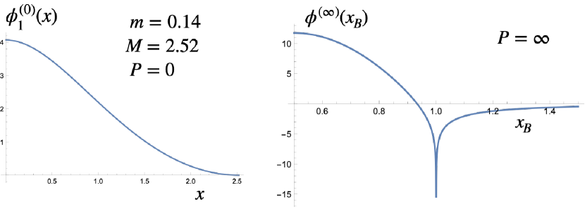
Figure 1: Features of the $\eta_{C}=-1$ ground state, with quark mass $m=0.14$ and bound state mass $M=2.51954$ $(V^{\prime}=1)$.
Left: Plot of rest frame wave function $\phi_{1}^{\scriptscriptstyle(P=0)}(x)$ (III.2) for $0\leq x\leq M$. $\phi^{\scriptscriptstyle{(0)}}_{1}(x\to\infty)$ oscillates according to (III.3).
Right: The IMF wave function $\phi^{\scriptscriptstyle{(\infty)}}({x_{B}})=\phi^{\scriptscriptstyle{(\infty)}}(1-{x_{B}})$ (71) for $0.5\leq{x_{B}}\leq 1.5$. $\phi^{\scriptscriptstyle{(\infty)}}({x_{B}}\to\infty)\simeq-0.40/x_{B}^{2}$.

V.2 Energy projection in the IMF

The spinors (45) simplify in the $P\to\infty$ limit. With $\varepsilon_{q}=1\ (-1)$ for $q>0\ (q<0)$,

$$U^{\scriptscriptstyle{(\infty)}}_{+}(q)=\frac{1}{\sqrt{2}}\Big{(}{\textstyle\begin{array}[]{c}1\\ \varepsilon_{q}\end{array}}\Big{)} \hskip 28.45274ptU^{\scriptscriptstyle{(\infty)}}_{-}(q)=\frac{1}{\sqrt{2}}\Big{(}{\textstyle\begin{array}[]{c}-\varepsilon_{q}\\ 1\end{array}}\Big{)}\hskip 28.45274ptV^{\scriptscriptstyle{(\infty)}}_{+}({\bar{q}})=\frac{1}{\sqrt{2}}\Big{(}{\textstyle\begin{array}[]{c}\varepsilon_{\bar{q}}\\ 1\end{array}}\Big{)}\hskip 28.45274ptV^{\scriptscriptstyle{(\infty)}}_{-}({\bar{q}})=\frac{1}{\sqrt{2}}\Big{(}{\textstyle\begin{array}[]{c}1\\ -\varepsilon_{\bar{q}}\end{array}}\Big{)}$$ (80)

$${U^{\scriptscriptstyle{(\infty)}}_{s}}^{\dagger}(q)(1+\alpha_{1}) =(1+s\varepsilon_{q})(1\ \ 1)\frac{1}{\sqrt{2}}\hskip 85.35826pt(1+\alpha_{1})V^{\scriptscriptstyle{(\infty)}}_{\bar{s}}({\bar{q}})=\frac{1}{\sqrt{2}}\Big{(}{\textstyle\begin{array}[]{c}1\\ 1\end{array}}\Big{)}(1+{\bar{s}}\varepsilon_{\bar{q}})$$ (83)

The energy projected ($s,{\bar{s}}=\pm$) wave function defined in (52) and (V.1) becomes, with $\phi^{\scriptscriptstyle(P\to\infty)}_{s{\bar{s}}}(k)\equiv\phi^{\scriptscriptstyle{(\infty)}}_{s{\bar{s}}}({x_{B}})$,

$$\phi^{\scriptscriptstyle{(\infty)}}_{s{\bar{s}}}({x_{B}}) \equiv\frac{1}{2m}\,\bar{U}_{s}^{\scriptscriptstyle{(\infty)}}(q)\Phi^{\scriptscriptstyle{(\infty)}}({x_{B}})V^{\scriptscriptstyle{(\infty)}}_{{\bar{s}}}(\bar{q})={U^{\scriptscriptstyle{(\infty)}}_{s}}^{\dagger}(p)(1+\alpha_{1})V^{\scriptscriptstyle{(\infty)}}_{\bar{s}}(\bar{p})\,\phi^{\scriptscriptstyle{(\infty)}}({x_{B}})={\textstyle\frac{1}{2}}(1+s\,\varepsilon_{q})(1+{\bar{s}}\,\varepsilon_{\bar{q}})\phi^{\scriptscriptstyle{(\infty)}}({x_{B}})$$ (84)

where $\varepsilon_{q}=\varepsilon_{x_{B}}$ since $q={x_{B}}P$, and similarly $\varepsilon_{\bar{q}}=\varepsilon_{1-{x_{B}}}$. Hence for $0<{x_{B}}<1$ only $\phi^{\scriptscriptstyle{(\infty)}}_{++}({x_{B}})$ is non-vanishing, while for ${x_{B}}<0$ only $\phi^{\scriptscriptstyle{(\infty)}}_{-+}({x_{B}})$ and for ${x_{B}}>1$ only $\phi^{\scriptscriptstyle{(\infty)}}_{+-}({x_{B}})$ are non-zero. The $\phi^{\scriptscriptstyle{(\infty)}}_{--}({x_{B}})$ component vanishes for all ${x_{B}}$ in the $P\to\infty$ limit at fixed $\tau_{P}$.

On the lhs. of the BSE (62) we may approximate $E_{P}=\sqrt{P^{2}+M^{2}}\simeq P+M^{2}/2P$, and similarly for $E_{q}$ and $E_{\bar{q}}$,

$$(E-sE_{q}-{\bar{s}}E_{{\bar{q}}})\phi^{\scriptscriptstyle{(\infty)}}_{s{\bar{s}}}({x_{B}})\simeq\Big{[}(1-s|{x_{B}}|-{\bar{s}}|(1-{x_{B}})|)P+\frac{1}{2P}\Big{(}M^{2}-s\,\frac{m^{2}}{|{x_{B}}|}-{\bar{s}}\,\frac{m^{2}}{|1-{x_{B}}|}\Big{)}\Big{]}\phi^{\scriptscriptstyle{(\infty)}}_{s{\bar{s}}}({x_{B}})$$ (85)

The form of $\phi^{\scriptscriptstyle{(\infty)}}_{s{\bar{s}}}({x_{B}})$ (84) ensures that the ${\cal O}\left(P\right)$ term vanishes in the $P\to\infty$ limit for all $s,{\bar{s}}=\pm$. The rhs. of the BSE (62) is, with $p={y_{B}}P$, $l=({y_{B}}-{\textstyle\frac{1}{2}})P$ and $\phi^{\scriptscriptstyle(P\to\infty)}_{s{\bar{s}}}(l)\equiv\phi^{\scriptscriptstyle{(\infty)}}_{s{\bar{s}}}({y_{B}})$,

$$-\frac{V^{\prime}}{\pi P}\mathchoice{{\vbox{\hbox{$\textstyle-$}}\kern-4.86108pt}}{{\vbox{\hbox{$\scriptstyle-$}}\kern-3.25pt}}{{\vbox{\hbox{$\scriptscriptstyle-$}}\kern-2.29166pt}}{{\vbox{\hbox{$\scriptscriptstyle-$}}\kern-1.875pt}}\!\int_{-\infty}^{\infty}\frac{d{y_{B}}}{({y_{B}}-{x_{B}})^{2}}\Big{[}\sum_{s^{\prime},{\bar{s}}^{\prime}=\pm}\Theta^{\scriptscriptstyle{(\infty)}}_{ss^{\prime}}(q,p)\phi^{\scriptscriptstyle{(\infty)}}_{s^{\prime}{\bar{s}}^{\prime}}({y_{B}})\Theta^{\scriptscriptstyle{(\infty)}}_{{\bar{s}}^{\prime}{\bar{s}}}({\bar{p}},{\bar{q}})-\phi^{\scriptscriptstyle{(\infty)}}_{s{\bar{s}}}({x_{B}})\Big{]}$$ (86)

The factors $\Theta^{\scriptscriptstyle{(\infty)}}_{ss^{\prime}}(q,p)={U^{\scriptscriptstyle{(\infty)}}_{s}}^{\dagger}(q)U^{\scriptscriptstyle{(\infty)}}_{s^{\prime}}(p)$ of (IV.2.2) and (80) in the IMF are,

$$\Theta^{\scriptscriptstyle{(\infty)}}_{++}(q,p) ={\textstyle\frac{1}{2}}(1+\varepsilon_{q}\varepsilon_{p})\hskip 59.75095pt\Theta^{\scriptscriptstyle{(\infty)}}_{+-}(q,p)={\textstyle\frac{1}{2}}(\varepsilon_{q}-\varepsilon_{p})$$

$$\Theta^{\scriptscriptstyle{(\infty)}}_{-+}(q,p) =-\Theta^{\scriptscriptstyle{(\infty)}}_{+-}(q,p)\hskip 56.9055pt\Theta^{\scriptscriptstyle{(\infty)}}_{--}(q,p)=\Theta^{\scriptscriptstyle{(\infty)}}_{++}(q,p)$$ (87)

For $0<{x_{B}}<1$ and $s={\bar{s}}=+$ we have in (85) $\phi^{\scriptscriptstyle{(\infty)}}_{++}({x_{B}})=2\phi^{\scriptscriptstyle{(\infty)}}({x_{B}})$ (84). Since $q>0$ and ${\bar{q}}>0$ the first term in (86) reduces to $2\phi^{\scriptscriptstyle{(\infty)}}({y_{B}})$ for all ${y_{B}}$,

$$\hskip-8.5359pt\sum_{s^{\prime},{\bar{s}}^{\prime}=\pm}\Theta^{\scriptscriptstyle{(\infty)}}_{+s^{\prime}}(q,p)\phi^{\scriptscriptstyle{(\infty)}}_{s^{\prime}{\bar{s}}^{\prime}}({y_{B}})\Theta^{\scriptscriptstyle{(\infty)}}_{{\bar{s}}^{\prime}+}({\bar{p}},{\bar{q}})=\left\{{\textstyle\begin{array}[]{l}\Theta^{\scriptscriptstyle{(\infty)}}_{+-}(q>0,p<0)\phi^{\scriptscriptstyle{(\infty)}}_{-+}({y_{B}}<0)\Theta^{\scriptscriptstyle{(\infty)}}_{++}({\bar{p}}>0,{\bar{q}}>0)=2\phi^{\scriptscriptstyle{(\infty)}}({y_{B}}<0)\\[5.69054pt] \Theta^{\scriptscriptstyle{(\infty)}}_{++}(q>0,p>0)\phi^{\scriptscriptstyle{(\infty)}}_{++}(0<{y_{B}}<1)\Theta^{\scriptscriptstyle{(\infty)}}_{++}({\bar{p}}>0,{\bar{q}}>0)=2\phi^{\scriptscriptstyle{(\infty)}}(0<{y_{B}}<1)\\[5.69054pt] \Theta^{\scriptscriptstyle{(\infty)}}_{++}(q>0,p>0)\phi^{\scriptscriptstyle{(\infty)}}_{+-}({y_{B}}>1)\Theta^{\scriptscriptstyle{(\infty)}}_{-+}({\bar{p}}<0,{\bar{q}}>0)=2\phi^{\scriptscriptstyle{(\infty)}}({y_{B}}>1)\end{array}}\right.$$ (91)

Consequently the BSE for the IMF wave function $\phi^{\scriptscriptstyle{(\infty)}}({x_{B}})$ of (71) is, for $0<{x_{B}}<1$ and $s={\bar{s}}=+$,

$$\Big{(}M^{2}-\frac{m^{2}}{{x_{B}}}-\frac{m^{2}}{1-{x_{B}}}\Big{)}\phi^{\scriptscriptstyle{(\infty)}}({x_{B}})=-\frac{2V^{\prime}}{\pi}\mathchoice{{\vbox{\hbox{$\textstyle-$}}\kern-4.86108pt}}{{\vbox{\hbox{$\scriptstyle-$}}\kern-3.25pt}}{{\vbox{\hbox{$\scriptscriptstyle-$}}\kern-2.29166pt}}{{\vbox{\hbox{$\scriptscriptstyle-$}}\kern-1.875pt}}\!\int_{-\infty}^{\infty}\frac{d{y_{B}}}{({y_{B}}-{x_{B}})^{2}}\,[\phi^{\scriptscriptstyle{(\infty)}}({y_{B}})-\phi^{\scriptscriptstyle{(\infty)}}({x_{B}})]$$ (92)

where $V^{\prime}={\textstyle\frac{1}{2}}g^{2}C_{F}$. This may be compared with Eq. (25) of ’t Hooft ’t Hooft (1974a), which multiplied with $g^{2}/\pi$ reads

$$\Big{(}M^{2}-\frac{m^{2}}{x}-\frac{m^{2}}{1-x}\Big{)}\phi(x)=-\frac{g^{2}}{\pi}\Big{(}\frac{1}{x}+\frac{1}{1-x}\Big{)}\phi(x)-\frac{g^{2}}{\pi}\mathchoice{{\vbox{\hbox{$\textstyle-$}}\kern-4.86108pt}}{{\vbox{\hbox{$\scriptstyle-$}}\kern-3.25pt}}{{\vbox{\hbox{$\scriptscriptstyle-$}}\kern-2.29166pt}}{{\vbox{\hbox{$\scriptscriptstyle-$}}\kern-1.875pt}}\!\int_{0}^{1}\frac{\phi(y)}{(y-x)^{2}}\,dy=-\frac{g^{2}}{\pi}\mathchoice{{\vbox{\hbox{$\textstyle-$}}\kern-4.86108pt}}{{\vbox{\hbox{$\scriptstyle-$}}\kern-3.25pt}}{{\vbox{\hbox{$\scriptscriptstyle-$}}\kern-2.29166pt}}{{\vbox{\hbox{$\scriptscriptstyle-$}}\kern-1.875pt}}\!\int_{0}^{1}\frac{\phi(y)-\phi(x)}{(y-x)^{2}}\,dy$$ (93)

The quark propagator corrections, which give rise to the terms $-(g^{2}/\pi)[1/x+1/(1-x)]\phi(x)$ in (93), decrease the singularity of the integral at $y=x$. There are no quark propagators in present approach, where the less singular form of the integral is a consequence of the Fourier transform (58). Identifying ’t Hooft’s coupling $g^{2}\to g^{2}C_{F}=2V^{\prime}$, $x\to{x_{B}}$ and $y\to{y_{B}}$ (93) agrees with (92), except that the negative energy components $\phi^{\scriptscriptstyle{(\infty)}}_{-+}(y_{B}<0)$ and $\phi^{\scriptscriptstyle{(\infty)}}_{+-}(y_{B}>1)$ extend the integration over ${y_{B}}$ from $[0,1]$ to $[-\infty,\infty]$.

The BSE (92) actually holds for all ${x_{B}}\neq 0,1$, i.e., $-\infty<{x_{B}}<\infty$. For ${x_{B}}<0,\ s=-,\ {\bar{s}}=+$,

$$\hskip-8.5359pt\sum_{s^{\prime},{\bar{s}}^{\prime}=\pm}\Theta^{\scriptscriptstyle{(\infty)}}_{-s^{\prime}}(q,p)\phi^{\scriptscriptstyle{(\infty)}}_{s^{\prime}{\bar{s}}^{\prime}}({y_{B}})\Theta^{\scriptscriptstyle{(\infty)}}_{{\bar{s}}^{\prime}+}({\bar{p}},{\bar{q}})=\left\{{\textstyle\begin{array}[]{l}\Theta^{\scriptscriptstyle{(\infty)}}_{--}(q<0,p<0)\phi^{\scriptscriptstyle{(\infty)}}_{-+}({y_{B}}<0)\Theta^{\scriptscriptstyle{(\infty)}}_{++}({\bar{p}}>0,{\bar{q}}>0)=2\phi^{\scriptscriptstyle{(\infty)}}({y_{B}}<0)\\[5.69054pt] \Theta^{\scriptscriptstyle{(\infty)}}_{-+}(q<0,p>0)\phi^{\scriptscriptstyle{(\infty)}}_{++}(0<{y_{B}}<1)\Theta^{\scriptscriptstyle{(\infty)}}_{++}({\bar{p}}>0,{\bar{q}}>0)=2\phi^{\scriptscriptstyle{(\infty)}}(0<{y_{B}}<1)\\[5.69054pt] \Theta^{\scriptscriptstyle{(\infty)}}_{-+}(q<0,p>0)\phi^{\scriptscriptstyle{(\infty)}}_{+-}({y_{B}}>1)\Theta^{\scriptscriptstyle{(\infty)}}_{-+}({\bar{p}}<0,{\bar{q}}>0)=2\phi^{\scriptscriptstyle{(\infty)}}({y_{B}}>1)\end{array}}\right.$$ (97)

Due to the symmetry $\phi^{\scriptscriptstyle{(\infty)}}({x_{B}})=-\eta_{C}\,\phi^{\scriptscriptstyle{(\infty)}}(1-{x_{B}})$ (V.1) the BSE (92) is unchanged when ${x_{B}}\to 1-{x_{B}}$. The singular behavior of the lhs. as ${x_{B}}\to 1$ is matched by a singularity on the rhs., since $\lim_{\epsilon\to 0}\phi^{\scriptscriptstyle{(\infty)}}({y_{B}}=1-\epsilon)\neq\lim_{\epsilon\to 0}\phi^{\scriptscriptstyle{(\infty)}}({y_{B}}=1+\epsilon)$. Table 1 demonstrates the validity of the BSE for the $\eta_{C}=-1$ ground state of Fig. 1.

Table 1: Numerical results for the BSE (92) at various values of ${x_{B}}$, for the bound state of Fig. 1. The second to fourth columns show the contributions to the right hand side from the indicated integration ranges over ${y_{B}}$. The full result for the rhs. (fifth column) agrees with the lhs. of (92) (last column).

$\ {x_{B}}\$	$\ -\infty<{y_{B}}<0\$	$\ 0<{y_{B}}<1\$	$\ 1<{y_{B}}<\infty\$	$\ -\infty<{y_{B}}<\infty\$	LHS of (92)
$-0.2\$	4.671	$-12.096$	$-0.328$	$-7.754$	$-7.754$
$0.5\$	16.338	41.025	16.335	73.698	73.698
$0.8\$	5.475	7.168	25.291	37.934	37.934
$0.9\$	1.810	$-19.004$	28.440	11.246	11.246
$0.99\$	$-3.051$	$-70.332$	49.712	$-23.672$	$-23.672$
$\ 0.999\$	$-6.043$	$-113.155$	253.917	134.719	134.719
$1.2\$	$-0.328$	$-12.096$	4.671	$-7.754$	$-7.754$
$1.5\$	0.010	$-4.759$	1.727	$-3.022$	$-3.022$

VI Using the temporal gauge constraint to determine $E_{a}$

VI.1 Reproducing the linear potential

The eigenvalue condition $H\left|{M,P}\right\rangle=E\left|{M,P}\right\rangle$ for the states $\left|{M,P}\right\rangle$ (6) of momentum $P$,

$$\left|{M,P}\right\rangle=\int dx_{q}dx_{\bar{q}}\,\bar{\psi}(x_{q})\mathbb{P}\exp\Big{[}ig\int_{x_{\bar{q}}}^{x_{q}}dx\,A_{a}(x)T_{a}\Big{]}\,\exp[iP(x_{q}+x_{\bar{q}})/2]\Phi^{\scriptscriptstyle{(P)}}(x_{q}-x_{\bar{q}})\psi(x_{\bar{q}})\left|{0}\right\rangle$$ (98)

determines the Bound State Equation (BSE) (22) for the wave function $\Phi^{\scriptscriptstyle{(P)}}(x_{q}-x_{\bar{q}})$. In Section II.3 the Hamiltonian $\hat{P}^{0}=H$ (14) was determined canonically from the QCD₂ action in temporal ($A^{0}=0$) gauge,

$$H=\int dx\,\big{[}{\textstyle\frac{1}{2}}(E_{a})^{2}+\psi^{\dagger}(-i\alpha_{1}{\buildrel\rightarrow\over{\partial}}_{x}+\gamma^{0}m-gA_{a}T^{a}\alpha_{1})\psi\big{]}$$ (99)

Physical states are required to be invariant under time-independent gauge transformations, which preserve $A^{0}=0$. Those transformations are generated by Gauss’ operator (4),

$$\mathcal{G}_{a}(t,x)\equiv\frac{\delta\mathcal{S}_{QCD}}{\delta{A_{a}^{0}(t,x)}}=\partial_{x}E_{a}(t,x)+gf_{abc}A_{b}E_{c}(t,x)-g\psi^{\dagger}T^{a}\psi(t,x)$$ (100)

In Section II.1 and Appendix A I verified that $\mathcal{G}_{a}(x)\left|{M,P}\right\rangle=0$. Hence

$$\partial_{x}E_{a}(x)\left|{M,P}\right\rangle=g\big{[}-f_{abc}A_{b}E_{c}(x)+\psi^{\dagger}T^{a}\psi(x)\big{]}\left|{M,P}\right\rangle\equiv g\,\mathcal{E}_{a}(x)\left|{M,P}\right\rangle$$ (101)

Viewed as a differential equation for $E_{a}(x)$ this provides an alternative expression for the $E_{a}^{2}$ contribution to $H$. Recalling that $\partial_{x}^{2}|x-y|=2\delta(x-y)$ we may solve for $E_{a}(x)$,

$$E_{a}(x)={\textstyle\frac{1}{2}}g\,\partial_{x}\int dy\,|x-y|\,\mathcal{E}_{a}(y)$$ (102)

The contribution of the color electric field to the Hamiltonian $H$ (99) is thus

$$H_{V}\equiv{\textstyle\frac{1}{2}}\int dx\,E_{a}^{2}(x) =\frac{g^{2}}{8}\int dx\Big{[}\partial_{x}\int dy\,|x-y|\,\mathcal{E}_{a}(y)\Big{]}\Big{[}\partial_{x}\int dz\,|x-x|\,\mathcal{E}_{a}(z)\Big{]}$$

$$=-\frac{g^{2}}{4}\int dy\,dz\,|y-z|\,\mathcal{E}_{a}(y)\,\mathcal{E}_{a}(z)$$ (103)

The fermion part $\psi^{\dagger}T^{a}\psi(x)$ of $\mathcal{E}_{a}(x)$ acting on the quark fields in $\left|{M,P}\right\rangle$ (98) gives,

$$\left[{\mathcal{E}_{a}(x)},{\bar{\psi}_{A}(x_{q})}\right]=\bar{\psi}_{A^{\prime}}(x_{q})T^{a}_{A^{\prime}A}\delta(x-x_{q})\hskip 56.9055pt\left[{\mathcal{E}_{a}(x)},{\psi_{A}(x_{\bar{q}})}\right]=-T^{a}_{AA^{\prime}}\psi_{A^{\prime}}(x_{\bar{q}})\delta(x-x_{\bar{q}})$$ (104)

The $-f_{abc}A_{b}E_{c}(x)$ term in $\mathcal{E}_{a}(x)$ (101) operating on the gauge link in $\left|{M,P}\right\rangle$ is suppressed by ${\cal O}\left(g\right)$ compared to the fermion contribution. Ignoring the gauge link contribution we have for a (globally) color singlet $q{\bar{q}}$ state,

$$\left|{q(x_{q}){\bar{q}}(x_{\bar{q}})}\right\rangle \equiv\sum_{A}\bar{\psi}_{A}^{\alpha}(x_{q})\psi_{A}^{\beta}(x_{\bar{q}})\left|{0}\right\rangle$$ (105)

$$H_{V}\left|{q(x_{q}){\bar{q}}(x_{\bar{q}})}\right\rangle ={\textstyle\frac{1}{2}}g^{2}|x_{q}-x_{\bar{q}}|\bar{\psi}(x_{q})T^{a}T^{a}\psi(x_{\bar{q}})\left|{0}\right\rangle={\textstyle\frac{1}{2}}g^{2}C_{F}|x_{q}-x_{\bar{q}}|\left|{q(x_{q}){\bar{q}}(x_{\bar{q}})}\right\rangle=V(x_{q}-x_{\bar{q}})\left|{q(x_{q}){\bar{q}}(x_{\bar{q}})}\right\rangle$$

The potential $V(x)={\textstyle\frac{1}{2}}g^{2}C_{F}|x|$ agrees with that previously obtained in (19), where it arose from the commutator of $E_{a}^{2}$ with the gauge link in $\left|{M,P}\right\rangle$.

VI.2 Adding a homogeneous solution to $E_{a}$

The electric fields generated by QED and QCD bound states differ in an important respect. The electric field $E(x)$ of QED₂ is given by (102) without a gauge boson or color matrix $T^{a}$ contribution,

$$E(x)={\textstyle\frac{1}{2}}e\,\partial_{x}\int dy\,|x-y|\,\psi_{e}^{\dagger}(y)\psi_{e}(y)={\textstyle\frac{1}{2}}e\int dy\,\varepsilon(x-y)\,\psi_{e}^{\dagger}(y)\psi_{e}(y)$$ (106)

where $\varepsilon(x)=1\ (-1)$ for $x>1\ (x<1)$. The electric field of an $e^{-}e^{+}$ state $\left|{e^{-}(x_{e})e^{+}(x_{\bar{e}})}\right\rangle\equiv\bar{\psi}_{e}^{\alpha}(x_{e})\psi_{e}^{\beta}(x_{\bar{e}})\left|{0}\right\rangle$ is

$$E(x)\left|{e^{-}(x_{e})e^{+}(x_{\bar{e}})}\right\rangle ={\textstyle\frac{1}{2}}e\big{[}\varepsilon(x-x_{e})-\varepsilon(x-x_{\bar{e}})\big{]}\left|{e^{-}(x_{e})e^{+}(x_{\bar{e}})}\right\rangle$$ (107)

The field is non-vanishing only between the charges. For $x_{e}>x_{\bar{e}}$,

$$\frac{\langle{e^{-}(x_{e})e^{+}(x_{\bar{e}})}|E(x)\left|{e^{-}(x_{e})e^{+}(x_{\bar{e}})}\right\rangle}{\langle{e^{-}(x_{e})e^{+}(x_{\bar{e}})}|e^{-}(x_{e})e^{+}(x_{\bar{e}})\rangle}=\left\{\begin{array}[]{l}-e\ \ \ (x_{\bar{e}}<x<x_{e})\\ \ 0\ \ \ \ \ \mbox{otherwise}\end{array}\right.$$ (110)

In QCD we have instead, from (102) and (104),

$$\langle{q(x_{q}){\bar{q}}(x_{\bar{q}})}|E_{a}(x)\left|{q(x_{q}){\bar{q}}(x_{\bar{q}})}\right\rangle\propto\mathrm{Tr}\,T^{a}=0\hskip 28.45274pt\mbox{for\ all}\ x$$ (111)

External observers see a vanishing color field due to the sum over quark colors. Equivalently, a color singlet state does not give rise to a color octet field. However, there is no sum over colors in the binding of a meson’s $q{\bar{q}}$ constituents. A red quark feels the color octet field generated by its anti-red anti-quark companion in the Fock state, and vice versa.

In $D=3+1$ dimensions Gauss’ law determines the (dipole) electric field of an $e^{+}e^{-}$ state. The solution is unique for fields that vanish at large distances, which is required to avoid long range interactions in QED. For color singlet $q\bar{q}$ states there is no such requirement, since the state does not generate a color octet field at any ${\boldsymbol{x}}$.

This motivates adding a homogeneous solution to (102), for which $\partial_{x}E_{a}(x)=0$,

$$E_{a}(x)=\partial_{x}\int dy\big{[}-\kappa\,x\,y+{\textstyle\frac{1}{2}}g\,|x-y|\big{]}\mathcal{E}_{a}(y)$$ (112)

The normalization $\kappa$ may depend on the state $\left|{M,P}\right\rangle$ that $E_{a}(x)$ acts on. Linearity in $x$ ensures that the homogeneous (sourceless) part of $E_{a}(x)$ is independent of $x$. Linearity in $y$ ensures translation invariance for color singlet states. After partial integrations $H_{V}={\textstyle\frac{1}{2}}\int dx\,E_{a}^{2}(x)$ becomes

$$H_{V}=\int dy\,dz\big{[}yz\big{(}{\textstyle\frac{1}{2}}\kappa^{2}{\textstyle\int}dx+g\kappa\big{)}-{\textstyle\frac{1}{4}}g^{2}|y-z|\big{]}\mathcal{E}_{a}(y)\mathcal{E}_{a}(z)$$ (113)

Acting on the state in (105) gives

$$H_{V}\left|{q(x_{q}){\bar{q}}(x_{\bar{q}})}\right\rangle=\big{[}({\textstyle\frac{1}{2}}\kappa^{2}{\textstyle\int}dx+g\kappa)C_{F}(x_{q}-x_{\bar{q}})^{2}+{\textstyle\frac{1}{2}}g^{2}C_{F}|x_{q}-x_{\bar{q}}|\big{]}\left|{q(x_{q}){\bar{q}}(x_{\bar{q}})}\right\rangle$$ (114)

The coefficient of $\kappa^{2}$ is proportional to the volume of space: the homogeneous contribution has introduced an isotropic vacuum field energy density $E_{\Lambda}$. This energy is irrelevant provided it is universal, i.e., the same for all states. Consequently we must take $\kappa^{2}$ to be inversely proportional to $(x_{q}-x_{\bar{q}})^{2}$. Defining the universal constant $\Lambda$ by

$$\kappa\equiv\frac{\Lambda^{2}}{gC_{F}}\,\frac{1}{|x_{q}-x_{\bar{q}}|}\hskip 56.9055ptE_{\Lambda}=\frac{\Lambda^{4}}{2g^{2}C_{F}}$$ (115)

gives, after subtracting the (infinite but universal) vacuum energy $E_{\Lambda}\int dx$,

$$H_{V}\left|{q(x_{q}){\bar{q}}(x_{\bar{q}})}\right\rangle=\big{(}\Lambda^{2}+{\textstyle\frac{1}{2}}g^{2}C_{F}\big{)}|x_{q}-x_{\bar{q}}|\left|{q(x_{q}){\bar{q}}(x_{\bar{q}})}\right\rangle$$ (116)

Inclusion of the homogeneous solution to $E_{a}(x)$ (112) added $\Lambda^{2}$ to the slope $V^{\prime}$ of the linear potential.

The possibility to include a homogeneous solution is potentially interesting in $D=3+1$ dimensions. It adds a linear term $V^{\prime}|{\boldsymbol{x}}|$ to the $-\alpha_{s}C_{F}/|{\boldsymbol{x}}|$ Coulomb $q{\bar{q}}$ potential, with $V^{\prime}$ related (as above) to the energy density of the vacuum. The corresponding potentials for color singlet $qqq$, $gg$ and $q{\bar{q}}g$ Fock states are also confining, and are correctly related to each other when the coordinates of two constituents coincide Hoyer (2021).

VII Discussion

Color confinement is a central feature of hadron dynamics. Numerical (lattice) calculations have determined that the hadron spectrum of QCD agrees with data Kronfeld (2012), whereas analytic methods remain elusive. Confinement has not been demonstrated using the formally exact Bethe-Salpeter Salpeter and Bethe (1951) approach to bound states. QCD₂ may provide insights since the Coulomb potential is confining in $D=1+1$ dimensions. ’t Hooft found ’t Hooft (1974a) that the Bethe-Salpeter equation of QCD₂ can be solved exactly in the $N_{c}\to\infty$ limit, which inspired many further studies.

The present study of the ’t Hooft model does not use the Bethe-Salpeter approach. This avoids quark propagators, which were found to be singular and to lack Lorentz covariance Bars and Green (1978). Instead, I directly determine the color singlet $\left|{q{\bar{q}}}\right\rangle$ eigenstates (6) of the QCD₂ Hamiltonian (14). Poincaré covariance emerges in an explicit, yet non-trivial way for these equal-time states. The ’t Hooft equation (93) is reproduced (92) with a surprising twist: The wave function $\phi^{\scriptscriptstyle{(\infty)}}({x_{B}})$ (71) has negative energy components even in the Infinite Momentum $(P\to\infty)$ Frame (IMF). Hence $\phi^{\scriptscriptstyle{(\infty)}}({x_{B}})$ does not vanish for ${x_{B}}\to 0,1$ as postulated by ’t Hooft (Fig. 1, right).

Negative energy solutions are familiar from the Dirac equation, but it may seem surprising that they survive in the IMF. Due to Lorentz contraction the potential is of ${\cal O}\left(1/P\right)$ while the kinetic energies are of ${\cal O}\left(P\right)$. However, the kinetic energy contributions to the BSE cancel at ${\cal O}\left(P\right)$ (85), leaving only ${\cal O}\left(1/P\right)$ terms in the ’t Hooft equation. A bound state constituent with negative kinetic energy in the rest frame will be boosted to a large negative energy in the IMF. This allows the energy and momentum ${x_{B}}P$ of a quark to be balanced by that of an anti-quark with $(1-{x_{B}})P$ even if ${x_{B}}>1$.

The reason for the difference with previous studies is not obvious, but could be due to boundary conditions. Feynman diagrams expand around free states with positive energy, whereas the $\left|{q{\bar{q}}}\right\rangle$ states (6) are confined by a linear potential. If the difference is due to boundary conditions this may be a lesson for confinement in $D=3+1$ dimensions. The confinement scale (which is absent from the action) can be introduced through a boundary condition (homogeneous solution) in the the determination of the instantaneous Coulomb potential, as seen above in Section VI.

The negative energy components allow an overlap $\langle{B\,C}|A\rangle$ between bound states $A,B$ and $C$, akin to the intuitive picture of $q{\bar{q}}$ creation in the confining potential (“string breaking”). This reminds of the duality in hadron dynamics, where parent states describe daughter states in an average sense. Since the potential is of leading ${\cal O}\left(g^{2}N_{c}\right)$ the overlap gives finite widths to the bound states even in the $N_{c}\to\infty$ limit.

Appendix A Gauge invariance of the bound states

Here I verify (12), $U_{G}\,\mathbb{P}(x_{\bar{q}}\to x_{q})U_{G}^{\dagger}=V(x_{q})\mathbb{P}(x_{\bar{q}}\to x_{q})V^{\dagger}(x_{\bar{q}})$, by discretizing in $x$ ($t=0$ is understood). For $x_{\bar{q}}\leq x\leq x_{q}$ and $0\leq n\leq N_{\mathbb{P}}$,

$$x\to y_{n} =x_{\bar{q}}+n\Delta{x}\hskip 56.9055pt\Delta{x}=\frac{x_{q}-x_{\bar{q}}}{N_{\mathbb{P}}}\hskip 56.9055pt\int_{x_{\bar{q}}}^{x_{q}}dx\,f(x)\to\Delta{x}\sum_{n=0}^{N_{\mathbb{P}}}f(y_{n})$$

$$\mathbb{P}(x_{\bar{q}}\to x_{q}) \equiv\mathbb{P}\exp\Big{[}ig\int_{x_{\bar{q}}}^{x_{q}}dx\,A_{a}(x)T_{a}\Big{]}=\prod_{n=0}^{N_{\mathbb{P}}}\exp\big{[}ig\Delta{x\,A_{a}(y_{n})T^{a}}\big{]}\hskip 28.45274pt(N_{\mathbb{P}}\to\infty)$$

$$=\prod_{n=l+1}^{N_{\mathbb{P}}}\exp\big{[}ig\Delta{x\,A_{a}(y_{n})T^{a}}\big{]}\Big{[}1+\Delta xigA_{a}(y_{l})T^{a}+{\cal O}\left((\Delta x)^{2}\right)\Big{]}\prod_{n=0}^{l-1}\exp\big{[}ig\Delta{x\,A_{a}(x_{n})T^{a}}\big{]}$$

$$=\mathbb{P}(y_{l}\to x_{q})\big{[}1+\Delta xigA_{a}(y_{l})T^{a}+{\cal O}\left((\Delta x)^{2}\right)\big{]}\mathbb{P}(x_{\bar{q}}\to y_{l})\hskip 28.45274pt(x_{\bar{q}}<y_{l}<x_{q})$$

$$\frac{\partial}{\partial x_{q}}\mathbb{P}(x_{\bar{q}}\to x_{q}) =igA_{a}(x_{q})T^{a}\mathbb{P}(x_{\bar{q}}\to x_{q})\hskip 28.45274pt\frac{\partial}{\partial x_{\bar{q}}}\mathbb{P}(x_{\bar{q}}\to x_{q})=-\mathbb{P}(x_{\bar{q}}\to x_{q})\,igA_{a}(x_{\bar{q}})T^{a}$$ (A.117)

The discretized derivative and the commutation relations (3) are,

$$\frac{\partial}{\partial{y_{k}}}f(y_{k}) =\frac{f(y_{k})-f(y_{k-1})}{\Delta x}$$ (A.118)

$$\left[{E_{a}(y_{k})},{A_{b}(y_{l})}\right]=\frac{i}{\Delta x}\delta_{k,l}\delta_{a,b} \hskip 56.9055pt\big{\{}{\psi^{\dagger}_{\alpha,A}(y_{k})},{\psi_{\beta,B}(y_{l})}\big{\}}=\delta_{\alpha,\beta}\delta_{A,B}\frac{\delta_{k.l}}{\Delta x}$$ (A.119)

The generator of time-independent gauge transformations $\mathcal{G}_{a}(t,x)$ is given in (4), the unitary transformation $U_{G}(t)$ in (10) and the unitary matrix $V_{\Lambda}(x)$ in (II.1). For $x_{\bar{q}}<y_{l},y_{l+1}<x_{q}$, using (A) and up to ${\cal O}\left(\Delta x\right)$ corrections,

$$\hskip-28.45274pt\left[{\frac{\partial}{\partial{y_{l}}}E_{a}(y_{l})},{\mathbb{P}(x_{\bar{q}}\to x_{q})}\right]=$$

$$=\frac{1}{\Delta x}\mathbb{P}(y_{l+2}\to x_{q})\left[{E_{a}(y_{l+1})-E_{a}(y_{l})},{\big{(}1+ig\Delta{x}A_{b}(y_{l+1})T^{b}\big{)}\big{(}1+ig\Delta{x}A_{c}(y_{l})T^{c}\big{)}}\right]\mathbb{P}(x_{\bar{q}}\to y_{l-1})$$

$$=\frac{1}{\Delta x}\mathbb{P}(y_{l+2}\to x_{q})\big{\{}i^{2}gT^{a}\big{(}1+ig\Delta{x}A_{b}(y_{l})T^{b}\big{)}-\big{(}1+ig\Delta{x}A_{b}(y_{l+1})T^{b}\big{)}i^{2}gT^{a}\big{\}}\mathbb{P}(x_{\bar{q}}\to y_{l-1})$$

$$=\mathbb{P}(y_{l}\to x_{q})i^{3}g^{2}A_{b}(y_{l})(T^{a}T^{b}-T^{b}T^{a})\mathbb{P}(x_{\bar{q}}\to y_{l})=\mathbb{P}(y_{l}\to x_{q})\,g^{2}f_{abc}A_{b}(y_{l})T^{c}\,\mathbb{P}(x_{\bar{q}}\to y_{l})$$

$$\hskip-28.45274pt\left[{gf_{abc}A_{b}E_{c}(y_{l})},{{\mathbb{P}(x_{\bar{q}}\to x_{q})}}\right]=\mathbb{P}(y_{l}\to x_{q})i^{2}g^{2}f_{abc}A_{b}(y_{l})T^{c}\,\mathbb{P}(x_{\bar{q}}\to y_{l})$$ (A.120)

The last two lines cancel in $\mathcal{G}_{a}(x)$,

$$\left[{\mathcal{G}_{a}(x)},{\mathbb{P}(x_{\bar{q}}\to x_{q})}\right]=0\hskip 28.45274pt\mathrm{for}\ \ x_{\bar{q}}<x<x_{q})$$ (A.121)

At the endpoints $y_{l}=x_{q}$ and $y_{l}=x_{\bar{q}}$ the derivative of the commutator is discontinuous,

$$\partial_{x_{q}}E_{a}(x_{q})\equiv\frac{E_{a}(x_{q}+\Delta x)-E_{a}(x_{q})}{\Delta x}\hskip 56.9055pt\partial_{x_{\bar{q}}}E_{a}(x_{\bar{q}})\equiv\frac{E_{a}(x_{\bar{q}})-E_{a}(x_{\bar{q}}-\Delta x)}{\Delta x}$$ (A.122)

and $\left[{E_{a}(x_{q}+\Delta x)},{\mathbb{P}(x_{\bar{q}}\to x_{q})}\right]=\left[{E_{a}(x_{\bar{q}}-\Delta x)},{\mathbb{P}(x_{\bar{q}}\to x_{q})}\right]=0$. Hence

$$\left[{\partial_{x_{q}}E_{a}(x_{q})},{\mathbb{P}(x_{\bar{q}}\to x_{q})}\right] =-\frac{1}{\Delta x}\left[{E_{a}(x_{q})},{\mathbb{P}(x_{\bar{q}}\to x_{q})}\right]=-\frac{i^{2}g}{\Delta x}T^{a}\mathbb{P}(x_{\bar{q}}\to x_{q})$$

$$\left[{\partial_{x_{\bar{q}}}E_{a}(x_{\bar{q}})},{\mathbb{P}(x_{\bar{q}}\to x_{q})}\right] =\frac{1}{\Delta x}\left[{E_{a}(x_{\bar{q}})},{\mathbb{P}(x_{\bar{q}}\to x_{q})}\right]=\frac{i^{2}g}{\Delta x}\mathbb{P}(x_{\bar{q}}\to x_{q})T^{a}$$ (A.123)

Analogously $\left[{gf_{abc}A_{b}E_{c}(x_{q}+\Delta x/2)},{\mathbb{P}(x_{\bar{q}}\to x_{q})}\right]=\left[{gf_{abc}A_{b}E_{c}(x_{\bar{q}}-\Delta x/2)},{\mathbb{P}(x_{\bar{q}}\to x_{q})}\right]=0$. Hence (12) is verified in the continuum limit,

$$\left[{\mathcal{G}_{a}(x)},{\mathbb{P}(x_{\bar{q}}\to x_{q})}\right] =\delta(x-x_{q})gT^{a}\,\mathbb{P}(x_{\bar{q}}\to x_{q})-\delta(x-x_{\bar{q}})\,\mathbb{P}(x_{\bar{q}}\to x_{q})gT^{a}$$

$$U_{G}\,\mathbb{P}(x_{\bar{q}}\to x_{q})U_{G}^{\dagger} =\mathbb{P}(x_{\bar{q}}\to x_{q})+i\int dx\,\left[{\mathcal{G}_{a}(x)},{\mathbb{P}(x_{\bar{q}}\to x_{q})}\right]\Lambda_{a}(x)$$

$$=[1+igT^{a}\Lambda_{a}(x_{q})]\mathbb{P}(x_{\bar{q}}\to x_{q})[1-igT^{a}\Lambda_{a}(x_{\bar{q}})]=V(x_{q})\mathbb{P}(x_{\bar{q}}\to x_{q})V^{\dagger}(x_{\bar{q}})$$ (A.124)

Appendix B Poincaré covariance

B.1 General definitions

In $D=1+1$ dimensions we may use a 2-dimensional Dirac algebra with Pauli matrices

$$\gamma^{0}=\sigma_{3}\hskip 56.9055pt\gamma^{1}=i\sigma_{2}\hskip 56.9055pt\gamma^{0}\gamma^{1}\equiv\alpha_{1}=\sigma_{1}$$ (B.125)

The unitary Poincaré operators are related to their generators as

$$U_{x}(\ell) =\exp(-i\ell\hat{P}^{1})\ \ \ \ \ \mbox{Space translation by\ }\ell$$ (B.126)

$$U_{t}(\tau) =\exp(i\tau\hat{P}^{0})\ \ \ \ \ \ \ \mbox{Time translation by\ }\tau$$ (B.127)

$$U_{tx}(\xi) =\exp(-i\xi\hat{M}^{01})\ \ \ \mbox{Boost by\ }\xi$$ (B.128)

The generators satisfy the equal-time Lie algebra

$$\left[{\hat{P}^{0}},{\hat{P}^{1}}\right]=0,\ \hskip 56.9055pt\left[{\hat{P}^{0}},{\hat{M}^{01}}\right]=i\hat{P}^{1},\ \hskip 56.9055pt\left[{\hat{P}^{1}},{\hat{M}^{01}}\right]=i\hat{P}^{0}$$ (B.129)

Infinitesimal translations of a field $\hat{\mathcal{O}}$ are generated by

$$\big{[}{\hat{P}^{1}},{\hat{\cal{O}}}\big{]} =i\partial_{x}\hat{\cal{O}}:\hskip 36.98866ptU_{x}(\delta{x})\hat{\cal{O}}U_{x}^{\dagger}(\delta{x})=\hat{\cal{O}}-i\delta{x}\big{[}{\hat{P}^{1}},{\hat{\cal{O}}}\big{]}=\hat{\cal{O}}+\delta{x}\,\partial_{x}\hat{\cal{O}}=\hat{\cal{O}}(x+\delta{x})$$

$$\big{[}{\hat{P}^{0}},{\hat{\cal{O}}}\big{]} =-i\partial_{t}\hat{\cal{O}}:\hskip 28.45274ptU_{t}(\delta{t})\hat{\cal{O}}U_{t}^{\dagger}(\delta{t})=\hat{\cal{O}}+i\delta{t}\big{[}{\hat{P}^{0}},{\hat{\cal{O}}}\big{]}=\hat{\cal{O}}+\delta{t}\,\partial_{t}\hat{\cal{O}}=\hat{\cal{O}}(t+\delta{t})$$ (B.130)

The Lie algebra ensures that the momentum and energy of a state $\left|{M,P}\right\rangle$, which satisfies $\hat{P}^{1}\left|{M,P}\right\rangle=P\left|{M,P}\right\rangle$ and $\hat{P}^{0}\left|{M,P}\right\rangle=E_{P}\left|{M,P}\right\rangle$, transform correctly under boosts,

$$\hat{P}^{1}(1-i\delta{\xi}\hat{M}^{01})\left|{M,P}\right\rangle =\big{\{}(1-i\delta{\xi}\hat{M}^{01})\hat{P^{1}}-i\delta{\xi}\big{[}{\hat{P^{1}}},{\hat{M}^{01}}\big{]}\big{\}}\left|{M,P}\right\rangle=(P+\delta{\xi}E_{P})(1-i\delta{\xi}\hat{M}^{01})\left|{M,P}\right\rangle$$

$$\hat{P}^{0}(1-i\delta{\xi}\hat{M}^{01})\left|{M,P}\right\rangle =\big{\{}(1-i\delta{\xi}\hat{M}^{01})\hat{P^{0}}-i\delta{\xi}\big{[}{\hat{P^{0}}},{\hat{M}^{01}}\big{]}\big{\}}\left|{M,P}\right\rangle=(E_{P}+\delta{\xi}P)(1-i\delta{\xi}\hat{M}^{01})\left|{M,P}\right\rangle$$ (B.131)

Hence we may identify $U_{tx}(\delta\xi)\left|{M,P}\right\rangle=\left|{M,P+\delta{\xi}E_{P}}\right\rangle$.

B.2 Generators of QCD₂ in temporal gauge

The translation invariance of the action defines the conserved energy-momentum tensor (see, e.g., Sections 7.3 and 7.4 of Weinberg (2005)). For a Lagrangian $\mathcal{L}$ (here given by (I)) depending on fields $\hat{\mathcal{O}}^{\ell}$ (here $A_{a}\equiv A_{a}^{1}$ and $\psi$),

$$T^{\nu}_{\ \mu} \equiv\frac{\partial\mathcal{L}}{\partial(\partial_{\nu}\hat{\mathcal{O}}^{\ell})}\,\partial_{\mu}\hat{\mathcal{O}}^{\ell}-g^{\nu}_{\mu}\,\mathcal{L}\hskip 56.9055pt\partial_{\nu}T^{\nu}_{\ \mu}=0$$ (B.132)

The generators of space and time translations are time independent. With $\alpha_{1}\equiv\gamma^{0}\gamma^{1}$,

$$\hat{P}^{1} \equiv\int dx\,T^{01}=-\int dx\,\frac{\partial\mathcal{L}_{QCD}}{\partial(\partial_{0}\hat{\mathcal{O}}^{\ell})}\partial_{1}\hat{\mathcal{O}}^{\ell}=\int dx\big{[}E_{a}{\buildrel\rightarrow\over{\partial}}_{x}A_{a}+\psi^{\dagger}(-i{\buildrel\rightarrow\over{\partial}}_{x})\psi\big{]}$$

$$\hat{P}^{0}=H \equiv\int dx\,T^{00}=\int dx\Big{[}\frac{\partial\mathcal{L}_{QCD}}{\partial(\partial_{0}\hat{\mathcal{O}}^{\ell})}\partial_{0}\hat{\mathcal{O}}^{\ell}-\mathcal{L}\Big{]}=\int dx\Big{\{}{\textstyle\frac{1}{2}}(E_{a})^{2}+\psi^{\dagger}\big{(}-i\alpha_{1}{\buildrel\rightarrow\over{\partial}}_{x}+\gamma^{0}m-g\alpha_{1}A_{a}T^{a}\big{)}\psi\Big{\}}$$ (B.133)

The boost generator $\hat{M}^{01}$ (B.128) may be expressed in terms of $\hat{P}^{1}$ and the (hermitian) Hamiltonian density $\mathcal{H}$ in (B.2),

$$\hat{M}^{01} =t\hat{P}^{1}-\int dx\,x\,\mathcal{H}=\int dx\Big{\{}t\big{[}E_{a}{\buildrel\rightarrow\over{\partial}}_{x}A_{a}+\psi^{\dagger}(-i{\buildrel\rightarrow\over{\partial}}_{x})\psi\big{]}-x\big{[}{\textstyle\frac{1}{2}}(E_{a})^{2}+\psi^{\dagger}(-i\alpha_{1}{\buildrel\leftrightarrow\over{\partial}}_{x}+\gamma^{0}m-g\alpha_{1}A_{a}T^{a})\psi\big{]}\Big{\}}$$

$$=\int dx\Big{\{}t\big{[}E_{a}{\buildrel\rightarrow\over{\partial}}_{x}A_{a}+\psi^{\dagger}(-i{\buildrel\rightarrow\over{\partial}}_{x})\psi\big{]}-x\big{[}{\textstyle\frac{1}{2}}(E_{a})^{2}+\psi^{\dagger}(-i\alpha_{1}{\buildrel\rightarrow\over{\partial}}_{x}+\gamma^{0}m-g\alpha_{1}A_{a}T^{a}+{\textstyle\frac{1}{2}}i\alpha_{1})\psi\big{]}\Big{\}}$$ (B.134)

where on the first line ${\buildrel\leftrightarrow\over{\partial}}={\textstyle\frac{1}{2}}({\buildrel\rightarrow\over{\partial}}-{\buildrel\leftarrow\over{\partial}})$ acts only on the fermion fields.

The Lie algebra (B.129) may be verified using the canonical commutation relations (3). More generally, all generators are independent of time, and the translation operators satisfy (B.1). Then

$$\big{[}{\hat{P}^{0}},{\hat{P}^{1}}\big{]} =-i\partial_{t}\hat{P}^{1}=0$$

$$\big{[}{\hat{P}^{1}},{\hat{M}^{01}}\big{]} =-\int dx\,x\,i\partial_{x}\mathcal{H}=\int dx\,i\mathcal{H}=i\hat{P}^{0}$$ (B.135)

The explicit time dependence of the boost generator $\hat{M}^{01}$ in (B.2) implies,

$$\frac{d}{dt}\hat{M}^{01} =\partial_{t}^{expl}\hat{M}^{01}+i\big{[}{\hat{P}^{0}},{\hat{M}^{01}}\big{]}=0$$

$$\big{[}{\hat{P}^{0}},{\hat{M}^{01}}\big{]} =i\partial_{t}^{expl}\hat{M}^{01}=i\hat{P}^{1}$$ (B.136)

B.3 Parity and charge conjugation

The fermion field may be expanded in the basis given by the free creation/annihilation operators,

$$\psi(t,x) =\int\frac{dk}{2\pi\,2E_{k}}\big{[}u(k)e^{-itE_{k}+ixk}\,b_{k}+v(k)e^{itE_{k}-ixk}\,d^{\dagger}_{k}\big{]}$$ (B.137)

$$u(k) =\frac{1}{\sqrt{E_{k}+m}}(E_{k}+m+\alpha_{1}k)\Big{(}{\textstyle\begin{array}[]{c}1\\ 0\end{array}}\Big{)}\hskip 91.04872ptE_{k}=\sqrt{k^{2}+m^{2}}$$ (B.140)

$$v(k) =\frac{1}{\sqrt{E_{k}+m}}(E_{k}+m+\alpha_{1}k)\Big{(}{\textstyle\begin{array}[]{c}0\\ 1\end{array}}\Big{)}=\alpha_{1}\,u(k)\hskip 48.36958pt\alpha_{1}=\gamma^{0}\gamma^{1}=\sigma_{1}$$ (B.143)

The parity transformation $(t,x)\to(t,-x)$ is implemented by the operator $\mathcal{P}$, which leaves the action (I) invariant,

$$\mathcal{P}\,b_{k}\,\mathcal{P}^{\dagger}=b_{k}\hskip 113.81102pt\mathcal{P}\,d_{k}\,\mathcal{P}^{\dagger}=-d_{k}$$

$$\mathcal{P}\,\psi(t,x)\,\mathcal{P}^{\dagger}=\gamma^{0}\psi(t,-x) \hskip 56.9055pt\mathcal{P}\,\bar{\psi}(t,x)\,\mathcal{P}^{\dagger}=\bar{\psi}(t,-x)\gamma^{0}\hskip 56.9055pt\mathcal{P}\,A^{1}_{a}(t,x)\,\mathcal{P}^{\dagger}=-A^{1}_{a}(t,-x)$$ (B.144)

For charge conjugation we have correspondingly, with $\gamma^{1}=\sigma_{3}\sigma_{1}=i\sigma_{2}$,

$$\mathcal{C}\,b_{k}\,\mathcal{C}^{\dagger}=d_{k}\hskip 113.81102pt\mathcal{C}\,d_{k}\,\mathcal{C}^{\dagger}=b_{k}$$

$$\mathcal{C}\,\psi(t,x)\,\mathcal{C}^{\dagger}=-\gamma^{1}{\bar{\psi}}^{T}(t,x) \hskip 42.67912pt\mathcal{C}\,\bar{\psi}(t,x)\,\mathcal{C}^{\dagger}=-{\psi}^{T}(t,x)\gamma^{1}\hskip 42.67912pt\mathcal{C}\,A^{1}_{a}(t,x)T^{a}\,\mathcal{C}^{\dagger}=-\big{[}A^{1}_{a}(t,x)T^{a}\big{]}^{T}$$ (B.145)

Appendix C $P$-dependence of $\Phi^{\scriptscriptstyle{(P)}}$ from $\hat{M}^{01}\left|{M,P}\right\rangle$

Here I verify that the $P$-dependence of the wave function determined by the BSE (22) agrees with that given by the boost generator $\hat{M}^{01}$ (B.2). Taking (6) to define $\left|{M,P}\right\rangle$ at $t=0$ I set $t=0$ in the expression (B.2) for $\hat{M}^{01}$,

$$\hat{M}^{01}(t=0)=\int dx\,\Big{\{}-x{\textstyle\frac{1}{2}}(E_{a})^{2}+\psi^{\dagger}\big{[}-x(-i\alpha_{1}{\buildrel\rightarrow\over{\partial}}_{x}+m\gamma^{0}-gA_{a}T^{a}\alpha_{1})+i{\textstyle\frac{1}{2}}\alpha_{1}\big{]}\psi\Big{\}}$$ (C.146)

The generator transforms the operators in $\left|{M,P}\right\rangle$ as follows,

$$\left[{\hat{M}^{01}},{\bar{\psi}_{\alpha}(x_{q})}\right] =\bar{\psi}(x_{q})\big{\{}-x_{q}(-i\alpha_{1}{\buildrel\leftarrow\over{\partial}}_{x_{q}}+m\gamma^{0}+\alpha_{1}gA_{a}(x_{q})T^{a})-{\textstyle\frac{1}{2}}i\alpha_{1}\big{\}}_{\alpha}$$

$$\left[{\hat{M}^{01}},{\psi_{\beta}(x_{\bar{q}})}\right] ={{}_{\beta}\big{\{}}x_{\bar{q}}(-i\alpha_{1}{\buildrel\rightarrow\over{\partial}}_{x_{\bar{q}}}+m\gamma^{0}-\alpha_{1}gA_{a}(x_{\bar{q}})T^{a})-{\textstyle\frac{1}{2}}i\alpha_{1}\big{\}}\psi(x_{\bar{q}})$$ (C.147)

$$\left[{\hat{M}^{01}},{\mathbb{P}(x_{\bar{q}}\to x_{q})}\right] =\int dx\left[{-{\textstyle\frac{1}{2}}xE_{a}^{2}},{\mathbb{P}(x_{\bar{q}}\to x_{q})}\right]=-{\textstyle\frac{1}{2}}\int_{x_{\bar{q}}}^{x_{q}}dx\,xg^{2}C_{F}\,\mathbb{P}(x_{\bar{q}}\to x_{q})=-{\textstyle\frac{1}{2}}(x_{q}^{2}-x_{\bar{q}}^{2})V^{\prime}\,\mathbb{P}(x_{\bar{q}}\to x_{q})$$

where I used (II.3) on the last line, and denoted $V^{\prime}\equiv{\textstyle\frac{1}{2}}g^{2}C_{F}$ (8). Altogether,

$$\hat{M}^{01}\left|{M,P}\right\rangle=\int dx_{q}dx_{\bar{q}}\,\bar{\psi}(x_{q})\Big{\{}$$

$$\big{[}-x_{q}(i\alpha_{1}{\buildrel\rightarrow\over{\partial}}_{x_{q}}+m\gamma^{0}+\alpha_{1}gA_{a}(x_{q})T^{a})-{\textstyle\frac{1}{2}}i\alpha_{1}\big{]}\mathbb{P}(x_{\bar{q}}\to x_{q})\,\exp[iP(x_{q}+x_{\bar{q}})/2]\Phi^{\scriptscriptstyle{(P)}}(x_{q}-x_{\bar{q}})$$

$$-{\textstyle\frac{1}{2}}(x_{q}^{2}-x_{\bar{q}}^{2})V^{\prime}\,\mathbb{P}(x_{\bar{q}}\to x_{q})\,\exp[iP(x_{q}+x_{\bar{q}})/2]\Phi^{\scriptscriptstyle{(P)}}(x_{q}-x_{\bar{q}})$$

$$+\mathbb{P}(x_{\bar{q}}\to x_{q})\,\exp[iP(x_{q}+x_{\bar{q}})/2]\Phi^{\scriptscriptstyle{(P)}}(x_{q}-x_{\bar{q}})\big{[}x_{\bar{q}}(i\alpha_{1}{\buildrel\leftarrow\over{\partial}}_{x_{\bar{q}}}+m\gamma^{0}-\alpha_{1}gA_{a}(x_{\bar{q}})T^{a})-{\textstyle\frac{1}{2}}i\alpha_{1}\big{]}$$

$$\hskip 284.52756pt\Big{\}}\psi(x_{\bar{q}})\left|{0}\right\rangle$$ (C.148)

As in (21) the derivatives acting on $\mathbb{P}(x_{\bar{q}}\to x_{q})$ are cancelled by the $\alpha_{1}gA_{a}T^{a}$ terms. For ${\buildrel\leftarrow\over{\partial}}_{x_{\bar{q}}}$ acting on $x_{\bar{q}}$,

$$-{\textstyle\frac{1}{2}}i\alpha_{1}\Phi^{\scriptscriptstyle{(P)}}+\Phi^{\scriptscriptstyle{(P)}}\big{[}i\alpha_{1}(x_{\bar{q}}{\buildrel\leftarrow\over{\partial}}_{x_{\bar{q}}})-{\textstyle\frac{1}{2}}i\alpha_{1}\big{]}=-{\textstyle\frac{1}{2}}i\left[{\alpha_{1}},{\Phi^{\scriptscriptstyle{(P)}}}\right]$$ (C.149)

With these simplifications,

$$\hat{M}^{01}\left|{M,P}\right\rangle =\int dx_{q}dx_{\bar{q}}\,\bar{\psi}(x_{q})\,\mathbb{P}(x_{\bar{q}}\to x_{q})\Big{\{}$$

$$-x_{q}(i\alpha_{1}{\buildrel\rightarrow\over{\partial}}_{x_{q}}+m\gamma^{0})\,\exp[iP(x_{q}+x_{\bar{q}})/2]\Phi^{\scriptscriptstyle{(P)}}(x_{q}-x_{\bar{q}})$$

$$-{\textstyle\frac{1}{2}}(x_{q}^{2}-x_{\bar{q}}^{2})V^{\prime}\,\exp[iP(x_{q}+x_{\bar{q}})/2]\Phi^{\scriptscriptstyle{(P)}}(x_{q}-x_{\bar{q}})-{\textstyle\frac{1}{2}}i\left[{\alpha_{1}},{\Phi^{\scriptscriptstyle{(P)}}}\right]$$

$$+\exp[iP(x_{q}+x_{\bar{q}})/2]\Phi^{\scriptscriptstyle{(P)}}(x_{q}-x_{\bar{q}})(i\alpha_{1}{\buildrel\leftarrow\over{\partial}}_{x_{\bar{q}}}+m\gamma^{0})x_{\bar{q}}\Big{\}}\psi(x_{\bar{q}})\left|{0}\right\rangle$$ (C.150)

$$\hskip-28.45274pt=\int dx_{q}dx_{\bar{q}}\,\bar{\psi}(x_{q})\,\mathbb{P}(x_{\bar{q}}\to x_{q})\,\exp[iP(x_{q}+x_{\bar{q}})/2]\Big{\{}$$

$$-ix_{q}\alpha_{1}{\buildrel\rightarrow\over{\partial}}_{x_{q}}\Phi^{\scriptscriptstyle{(P)}}(x_{q}-x_{\bar{q}})-ix_{\bar{q}}{\buildrel\rightarrow\over{\partial}}_{x_{q}}\Phi^{\scriptscriptstyle{(P)}}(x_{q}-x_{\bar{q}})\alpha_{1}+{\textstyle\frac{1}{2}}x_{q}P\alpha_{1}\Phi^{\scriptscriptstyle{(P)}}-{\textstyle\frac{1}{2}}x_{\bar{q}}P\Phi^{\scriptscriptstyle{(P)}}\alpha_{1}$$

$$-x_{q}m\gamma^{0}\Phi^{\scriptscriptstyle{(P)}}+x_{\bar{q}}m\Phi^{\scriptscriptstyle{(P)}}\gamma^{0}-{\textstyle\frac{1}{2}}V^{\prime}(x_{q}-x_{\bar{q}})(x_{q}+x_{\bar{q}})\,\Phi^{\scriptscriptstyle{(P)}}-{\textstyle\frac{1}{2}}i\left[{\alpha_{1}},{\Phi^{\scriptscriptstyle{(P)}}}\right]\Big{\}}\psi(x_{\bar{q}})\left|{0}\right\rangle$$ (C.151)

With $x\equiv x_{q}-x_{\bar{q}}$, replace

$$x_{q}={\textstyle\frac{1}{2}}(x_{q}+x_{\bar{q}})+{\textstyle\frac{1}{2}}x\hskip 56.9055ptx_{\bar{q}}={\textstyle\frac{1}{2}}(x_{q}+x_{\bar{q}})-{\textstyle\frac{1}{2}}x\hskip 56.9055pt\partial_{x_{q}}\Phi^{\scriptscriptstyle{(P)}}(x_{q}-x_{\bar{q}})=\partial_{x}\Phi^{\scriptscriptstyle{(P)}}(x)$$ (C.152)

Use the bound state equation (22) on the terms $\propto x_{q}+x_{\bar{q}}$,

$$-{\textstyle\frac{1}{2}}(x_{q}+x_{\bar{q}})\Big{(}i\partial_{x}\left\{{\alpha_{1}},{\Phi^{\scriptscriptstyle{(P)}}(x)}\right\}-{\textstyle\frac{1}{2}}P\left[{\alpha_{1}},{\Phi^{\scriptscriptstyle{(P)}}(x)}\right]+m\left[{\gamma^{0}},{\Phi^{\scriptscriptstyle{(P)}}(x)}\right]+V^{\prime}x\Phi^{\scriptscriptstyle{(P)}}(x)\Big{)}=-{\textstyle\frac{1}{2}}(x_{q}+x_{\bar{q}})E_{P}\Phi^{\scriptscriptstyle{(P)}}(x)$$ (C.153)

giving

$$\hat{M}^{01}\left|{M,P}\right\rangle =\int dx_{q}dx_{\bar{q}}\,\bar{\psi}(x_{q})\,\mathbb{P}(x_{q},x_{\bar{q}})\,\exp[iP(x_{q}+x_{\bar{q}})/2]\Big{\{}$$

$$-{\textstyle\frac{1}{2}}(x_{q}+x_{\bar{q}})E_{P}\Phi^{\scriptscriptstyle{(P)}}-{\textstyle\frac{1}{2}}ix\partial_{x}\left[{\alpha_{1}},{\Phi^{\scriptscriptstyle{(P)}}}\right]+{\textstyle\frac{1}{4}}xP\left\{{\alpha_{1}},{\Phi^{\scriptscriptstyle{(P)}}}\right\}-{\textstyle\frac{1}{2}}xm\left\{{\gamma^{0}},{\Phi^{\scriptscriptstyle{(P)}}}\right\}-{\textstyle\frac{1}{2}}i\left[{\alpha_{1}},{\Phi^{\scriptscriptstyle{(P)}}}\right]\Big{\}}\psi(x_{\bar{q}})\left|{0}\right\rangle$$ (C.154)

According to Eq. (A.93) of Hoyer (2021) the BSE (22) implies

$$-i{\textstyle\frac{1}{2}}x\partial_{x}\left[{\alpha_{1}},{\Phi^{\scriptscriptstyle{(P)}}}\right]+{\textstyle\frac{1}{4}}xP\left\{{\alpha_{1}},{\Phi^{\scriptscriptstyle{(P)}}}\right\}-{\textstyle\frac{1}{2}}xm\left\{{\gamma^{0}},{\Phi^{\scriptscriptstyle{(P)}}}\right\}=\frac{ixP}{E_{P}-V}\partial_{x}\Phi^{\scriptscriptstyle{(P)}}-\frac{iV^{\prime}x}{2(E_{P}-V)}\left[{\alpha_{1}},{\Phi^{\scriptscriptstyle{(P)}}}\right]$$ (C.155)

Use this in (C) to obtain

$$\hat{M}^{01}\left|{M,P}\right\rangle=\int dx_{q}dx_{\bar{q}}\, \bar{\psi}(x_{q})\,\mathbb{P}(x_{q},x_{\bar{q}})\,\exp[iP(x_{q}+x_{\bar{q}})/2]\Big{\{}$$

$$-{\textstyle\frac{1}{2}}(x_{q}+x_{\bar{q}})E_{P}\Phi^{\scriptscriptstyle{(P)}}+\frac{ixP}{E_{P}-V}\partial_{x}\Phi^{\scriptscriptstyle{(P)}}-\frac{iE_{P}}{2(E_{P}-V)}\left[{\alpha_{1}},{\Phi^{\scriptscriptstyle{(P)}}}\right]\Big{\}}\psi(x_{\bar{q}})\left|{0}\right\rangle$$ (C.156)

From the definition of $\hat{M}^{01}$ in (B.128), using $\partial_{\xi}P=E_{P}$,

$$U_{tx}(\delta{\xi})\left|{M,P}\right\rangle= (1-i\delta{\xi}\hat{M}^{01})\left|{M,P}\right\rangle$$ (C.157)

$$-i\hat{M}^{01}\left|{M,P}\right\rangle=\frac{\delta}{\delta{\xi}}\left|{M,P}\right\rangle= \frac{\delta}{\delta{\xi}}\int dx_{q}dx_{\bar{q}}\,\bar{\psi}(x_{q})\mathbb{P}\exp\Big{[}ig\int_{x_{\bar{q}}}^{x_{q}}dx\,A_{a}(x)T_{a}\Big{]}\,\exp[{\textstyle\frac{1}{2}}iP(x_{q}+x_{\bar{q}})]\Phi^{\scriptscriptstyle{(P)}}(x_{q}-x_{\bar{q}})\psi(x_{\bar{q}})\left|{0}\right\rangle$$

$$=\int dx_{q}dx_{\bar{q}}\,\bar{\psi}(x_{q})\mathbb{P}\exp \Big{[}ig\int_{x_{\bar{q}}}^{x_{q}}dx\,A_{a}(x)T_{a}\Big{]}\,\exp[iP(x_{q}+x_{\bar{q}})/2]\Big{\{}{\textstyle\frac{1}{2}}iE_{P}(x_{q}+x_{\bar{q}})\Phi^{\scriptscriptstyle{(P)}}+\partial_{\xi}\Phi^{\scriptscriptstyle{(P)}}\Big{\}}\psi(x_{\bar{q}})\left|{0}\right\rangle$$ (C.158)

Comparing with (C) implies that $\hat{M}^{01}$ generates the following change of $\Phi^{\scriptscriptstyle{(P)}}(x)$,

$$\partial_{\xi}\Phi^{\scriptscriptstyle{(P)}}(x)=\frac{xP}{E_{P}-V}\partial_{x}\Phi^{\scriptscriptstyle{(P)}}-\frac{E_{P}}{2(E_{P}-V)}\left[{\alpha_{1}},{\Phi^{\scriptscriptstyle{(P)}}}\right]$$ (C.159)

This agrees with Eq. (7.32) of Hoyer (2021), which was derived from the $P$-dependence of the solution of the BSE. Hence the $P$-dependence induced by the boost agrees with that implied by the BSE (22), confirming the analysis in Dietrich et al. (2012).

References

- ’t Hooft (1974a) G. ’t Hooft, Nucl. Phys. B 75, 461 (1974a).
- Callan et al. (1976) C. G. Callan, Jr., N. Coote, and D. J. Gross, Phys. Rev. D 13, 1649 (1976).
- Einhorn (1976) M. B. Einhorn, Phys. Rev. D 14, 3451 (1976).
- Einhorn et al. (1977) M. B. Einhorn, S. Nussinov, and E. Rabinovici, Phys. Rev. D 15, 2282 (1977).
- Brower et al. (1977) R. C. Brower, J. R. Ellis, M. G. Schmidt, and J. H. Weis, Nucl. Phys. B 128, 131 (1977).
- ’t Hooft (1974b) G. ’t Hooft, Nucl. Phys. B 72, 461 (1974b).
- Witten (1979) E. Witten, Nucl. Phys. B 160, 57 (1979).
- Bars and Green (1978) I. Bars and M. B. Green, Phys. Rev. D 17, 537 (1978).
- Li et al. (1987) M. Li, L. Wilets, and M. C. Birse, J. Phys. G 13, 915 (1987).
- Jia et al. (2017) Y. Jia, S. Liang, L. Li, and X. Xiong, JHEP 11, 151 (2017), arXiv:1708.09379 [hep-ph] .
- Hamer (1982) C. J. Hamer, Nucl. Phys. B 195, 503 (1982).
- Berruto et al. (2002) F. Berruto, L. Giusti, C. Hoelbling, and C. Rebbi, Phys. Rev. D 65, 094516 (2002), arXiv:hep-lat/0201010 .
- García Pérez et al. (2016) M. García Pérez, A. González-Arroyo, L. Keegan, and M. Okawa, PoS LATTICE2016, 337 (2016), arXiv:1612.07380 [hep-lat] .
- Willemsen (1978) J. F. Willemsen, Phys. Rev. D17, 574 (1978).
- Bjorken (1979) J. D. Bjorken, in Quantum chromodynamics: Proceedings, 7th SLAC Summer Institute on Particle Physics (SSI 79), Stanford, Calif., 9-20 Jul 1979 (1979) p. 219.
- Leibbrandt (1987) G. Leibbrandt, Rev. Mod. Phys. 59, 1067 (1987).
- Strocchi (2013) F. Strocchi, Int. Ser. Monogr. Phys. 158, 1 (2013).
- Christ and Lee (1980) N. H. Christ and T. D. Lee, Phys. Rev. D22, 939 (1980).
- Weinberg (2005) S. Weinberg, The Quantum theory of fields. Vol. 1: Foundations (Cambridge University Press, 2005).
- Salpeter and Bethe (1951) E. E. Salpeter and H. A. Bethe, Phys. Rev. 84, 1232 (1951).
- Chodos et al. (1974) A. Chodos, R. Jaffe, K. Johnson, C. B. Thorn, and V. Weisskopf, Phys. Rev. D 9, 3471 (1974).
- Hoyer (2021) P. Hoyer, Journey to the Bound States, SpringerBriefs in Physics (Springer, 2021) arXiv:2101.06721 [hep-ph] .
- Peskin and Schroeder (1995) M. E. Peskin and D. V. Schroeder, An Introduction to quantum field theory (Addison-Wesley, Reading, USA, 1995).
- Dietrich et al. (2013) D. D. Dietrich, P. Hoyer, and M. Järvinen, Phys. Rev. D87, 065021 (2013), arXiv:1212.4747 [hep-ph] .
- Dietrich et al. (2012) D. D. Dietrich, P. Hoyer, and M. Järvinen, Phys. Rev. D85, 105016 (2012), arXiv:1202.0826 [hep-ph] .
- Plesset (1932) M. S. Plesset, Phys. Rev. 41, 278 (1932).
- Melnitchouk et al. (2005) W. Melnitchouk, R. Ent, and C. Keppel, Phys. Rept. 406, 127 (2005), arXiv:hep-ph/0501217 .
- Kronfeld (2012) A. S. Kronfeld, Ann. Rev. Nucl. Part. Sci. 62, 265 (2012), arXiv:1203.1204 [hep-lat] .