Linear and uniform in time bound for the binary branching model with Moran type interactions

Abstract

In this note, we recall the definition of the binary branching model with Moran type interactions (BBMMI) introduced in [8]. In this interacting particle system, particles evolve, reproduce and die independently and, with a probability that may depend on the configuration of the whole system, the death of a particle may trigger the reproduction of another particle, while a branching event may trigger the death of another particle. We recall its relation to the Feynman-Kac semigroup of the underlying Markov evolution and improve on the $\displaystyle L^{2}$ distance between their normalisations proved in [8], when additional regularity is assumed on the process.

Keywords : interacting particle systems, branching processes, many-to-one, Markov processes, Brownian motion with drift, Moran model.

MSC: 82C22, 82C80, 65C05, 60J25, 92D25, 60J80.

1 Introduction

Branching processes and Moran-type models represent two distinct but complementary approaches to studying population dynamics and related phenomena. Moran-type processes, introduced by Moran [28], are particularly suited for modeling finite populations influenced by mechanisms such as genetic drift, mutation, and natural selection, which can either enhance or diminish genetic diversity. The Moran model describes a system of $\displaystyle N$ genes where, at random exponential intervals, two particles are chosen uniformly: one is removed while the other is duplicated, breaking the independence between particles. For an in-depth exploration of this model and its generalisations, we refer the reader to [17] and references therein. Furthermore, this resampling approach has been employed in various models of particle systems for the numerical solution of Feynman-Kac formulae [6, 14, 13, 32].

On the other hand, branching processes naturally model systems where events such as branching and killing occur independently. These processes arise in contexts such as population size dynamics [22, 23, 26], neutron transport [7], genetic evolution [27], growth-fragmentation phenomena [2, 1], and cell proliferation kinetics [33]. They are also studied for their theoretical properties [22, 10, 19, 20, 21], with a particular focus on their multiplicative behavior, scaling properties, and asymptotic dynamics over long time scales.

In [8], a new model has been proposed, which encompasses both the Moran model and binary branching processes. In this article, the authors consider a particle system with (natural) branching and killing, as well as Moran type interactions. More precisely, when the system is initiated from $\displaystyle N$ particles, each particle evolves according to an independent copy of a given Markov process, $\displaystyle X$, until either a (binary) branching or killing event occurs. Here, binary refers to the fact that the particle is replaced by exactly two independent copies of itself. If such a branching event occurs, with a probability that may depend on the configuration of the whole system, another particle is removed from the system according to a selection mechanism. Similarly, if a killing event occurs, with a probability which may also depend on the configuration of the whole system, another particle is duplicated via a resampling mechanism. We refer to this model as the binary branching model with Moran interactions, or BBMMI for short.

In the present paper, we will, for simplicity, only consider the so called $\displaystyle N_{min}-N_{max}$ model, which is the BBMMI model with a particular choice of selection and resampling mechanisms. Indeed, the $\displaystyle N_{min}-N_{max}$ model is a binary branching process whose population size is constrained to remain in $\displaystyle\{N_{min},\ldots,N_{max}\}$, where $\displaystyle 2\leq N_{min}\leq N_{max}<+\infty$ are fixed. In order to constrain the size of the process, when the size of the population reaches $\displaystyle N_{max}$ (resp. $\displaystyle N_{min}$) and a natural branching (resp. killing) event occurs, we set the probability of selection (resp. resampling) to be $\displaystyle 1$. As will be clear, our results extend to the more general situations under the appropriate regularity assumptions.

The main contributions of [8] are two-fold. First, an explicit relation between the average of the empirical distribution of the particle system and the average of the underlying Markov process $\displaystyle X$. Letting $\displaystyle m_{T}$ denote the empirical distribution of the particle system at time $\displaystyle T$, and $\displaystyle Q_{T}$ denote the first moment of the underlying binary branching process without selection and resampling, the authors show that for any $\displaystyle T\geq 0$,

$$\mathbb{E}\left[\Pi_{T}^{A}\,\Pi_{T}^{B}m_{T}(f)\right]=m_{0}Q_{T}(f),$$ (1)

where $\displaystyle\Pi_{T}^{A}$ and $\displaystyle\Pi_{T}^{B}$ are stochastic weights that compensate for the resampling and selection events that occur up to time $\displaystyle T$. Second, that after normalisation, we can give explicit bounds on the difference between the empirical particle system and the corresponding semigroup:

$$\left\|\frac{m_{0}Q_{T}(f)}{m_{0}Q_{T}(\mathbf{1}_{E})}-\frac{m_{T}(f)}{m_{T}(\mathbf{1}_{E})}\right\|_{2}\leq C\,\exp(c\|b\|_{\infty}T)\frac{\|f\|_{\infty}}{m_{0}Q_{T}(\mathbf{1}_{E})/{N_{0}}}\,\frac{1}{\sqrt{N_{0}}},$$ (2)

where $\displaystyle m_{0}(\mathbf{1}_{E})=N_{0}$ and $\displaystyle C,c$ are positive constants.

As the reader will notice, the above bound is exponential in $\displaystyle T$, which is partly due to the generality of the setting considered in [8]. The aim of the present note is to state and prove that, under suitable regularity condition, this bound can be chosen linear in $\displaystyle T$.

We also mention that bounds for $\displaystyle L^{2}$ norms of the form given above have been studied in detail for interacting particle systems with constant size. We refer the reader to [11, 12, 29, 25] and references therein for further details.

The rest of the article is set out as follows. In section 2, we recall the $\displaystyle N_{min}-N_{max}$ model introduced in [8], along with some useful notation that will be used throughout the rest of the article. In section 3, we give our main result that strengthens the bound (2) obtained in [8], followed by a discussion of the implications of this result. Finally, in section 4 we discuss the case of Brownian motion with drift evolving in a bounded domain with $\displaystyle C^{2}$ boundary. The purpose of this section is to prove that the $\displaystyle L^{2}$ distance between the (normalised) semigroup associated with the branching Brownian motion with drift and the approximating $\displaystyle N_{min}-N_{max}$ model can be optimally bounded by $\displaystyle C/\sqrt{N_{min}}$.

2 Description of the model

Let $\displaystyle(\Omega,\mathcal{F},(X_{t})_{t\in[0,+\infty)})$ be a continuous time progressively measurable Markov process with values in a measurable state space $\displaystyle E$. We denote by $\displaystyle{\mathbf{P}}_{x}$ its law when initiated at $\displaystyle x\in E$ and by $\displaystyle{\mathbf{E}}_{x}$ the corresponding expectation operator. We also allow for the possibility that the Markov process $\displaystyle X$ is absorbed, or killed, in the sense that we consider a cemetery state $\displaystyle\partial\notin E$ such that $\displaystyle X_{t}\in\{\partial\}$ for all $\displaystyle t\geq\tau_{\partial}:=\inf\{t\geq 0:X_{t}\in\{\partial\}\}$. We extend, whenever necessary, any measurable function $\displaystyle f:E\to[0,+\infty)$ by $\displaystyle f\equiv 0$ on $\displaystyle{\partial}$. We call this ‘hard killing’ to distinguish with the notion of ‘soft killing’ introduced below.

We further introduce functions $\displaystyle b:E\to\mathbb{R}_{+}$ and $\displaystyle\kappa:E\to\mathbb{R}_{+}$, that denote the branching and (soft) killing rate of the Markov process. With this notation, we introduce the semigroup

$$\displaystyle Q_{t}f(x) \displaystyle={\mathbf{E}}_{x}\left[f(X_{t})\exp\left(\int_{0}^{t}(b(X_{s})-\kappa(X_{s}))\,{\rm d}s\right){\mathbf{1}}_{t<\tau_{\partial}}\right],$$

defined for all bounded measurable functions $\displaystyle f:E\to\mathbb{R}$, $\displaystyle t\geq 0$ and $\displaystyle x\in E$, This defines a Feynman-Kac semigroup $\displaystyle(Q_{t})_{t\geq 0}$, which is related to the binary branching model where particles move as copies of $\displaystyle X$ that are killed at rate $\displaystyle\kappa$ and branch at rate $\displaystyle b$ resulting in the creation of two independent copies of the original particle. The relation between $\displaystyle Q$ and this process is given by the well-known many-to-one formula, see for instance [18] and references therein, and it has been extended to the BBMMI in [8].

Before describing the interacting particle system associated with the branching process described above, we first introduce the following assumptions.

Assumption 1.

The branching rate $\displaystyle b$ is uniformly bounded.

Assumption 2.

For any $\displaystyle x\in E$ and $\displaystyle t\in[0,+\infty)$, $\displaystyle{\mathbf{P}}_{x}(\tau_{\partial}=t)=0$ and $\displaystyle\inf_{x\in E}{\mathbf{P}}_{x}(\tau_{\partial}>t)>0$.

We now recall the algorithmic description of the dynamics of the BBMMI particle system in the particular setting of the $\displaystyle N_{min}-N_{max}$ model with branching and killing rates $\displaystyle b$ and $\displaystyle\kappa$. The formal construction of the process is a non-trivial task, and is given in the supplementary material [9] of [8]. To this end, let $\displaystyle 2\leq N_{min}\leq N_{max}<\infty$, and fix $\displaystyle{N}_{0}\in\{N_{min},\ldots,N_{max}\}$. We consider the particle system $\displaystyle((X^{i}_{t})_{i\in N_{t}})_{t\in[0,+\infty)}$, where $\displaystyle N_{t}$ is the number of particles in the system at time $\displaystyle t$.

Evolution of the $\displaystyle N_{min}-N_{max}$ model.

1. The particles $\displaystyle X^{i}$, $\displaystyle i\in\{1,\ldots,N_{0}\}$, evolve as independent copies of $\displaystyle X$, and we consider the following times:

   $$\displaystyle\tau^{b,i}_{1}:=\inf\{t\geq 0,\ \int_{0}^{t}b(X^{i}_{s})\,ds\geq e_{1}^{i,b}\},$$

   and

   $$\displaystyle\tau^{\kappa,i}_{1}:=\inf\{t\geq 0,\ \int_{0}^{t}\kappa(X^{i}_{s})\,ds\geq e_{1}^{i,\kappa}\},$$

   and

   $$\displaystyle\tau^{{\partial},i}_{1}:=\inf\{t\geq 0,\ X^{i}_{t}\in{\partial}\},$$

   where $\displaystyle e_{1}^{i,b},e_{1}^{i,\kappa}$, $\displaystyle i=1,\dots,{N}_{0}$ are exponential random variables with parameter $\displaystyle 1$, and are independent of each other and everything else.

2. Denoting by $\displaystyle i_{0}$ the index of the (unique) particle such that $\displaystyle\tau^{b,i_{0}}_{1}\wedge\tau^{\kappa,i_{0}}_{1}\wedge\tau^{\partial,i_{0}}_{1}=\tau_{1}$, where $\displaystyle\tau_{1}=\min_{i\in\bar{S}_{0}}\tau^{b,i}_{1}\wedge\tau^{\kappa,i}_{1}\wedge\tau^{\partial,i}_{1}$, we have $\displaystyle N_{t}=N_{0}$ for all $\displaystyle t<\tau_{1}$ and

   1. if $\displaystyle\tau_{1}=\tau^{b,i_{0}}_{1}$, then a branching event occurs;

   2. if $\displaystyle\tau_{1}=\tau^{\kappa,i_{0}}_{1}$, then a soft killing event occurs;

   3. if $\displaystyle\tau_{1}=\tau^{{\partial},i_{0}}_{1}$, then a hard killing event occurs.

3. Then a resampling or selection event may occur, depending on the following situations.

   1. Killing. If a (soft or hard) killing event occurred at the preceding step, then we say that $\displaystyle i_{0}$ is killed at time $\displaystyle\tau_{1}$ and we consider the following further two cases.

      • If the total number of particles, $\displaystyle N_{0}$, is equal to $\displaystyle N_{min}$, particle $\displaystyle i_{0}$ is removed from the system and a resampling event occurs: choose $\displaystyle j_{0}$ uniformly from $\displaystyle\{1,\ldots,N_{0}\}\setminus\{i_{0}\}$ and set

        $$X^{i_{0}}_{\tau_{1}}:=X^{j_{0}}_{\tau_{1}}.$$

        Observe that the number of particles in the system at time $\displaystyle\tau_{1}$ is then $\displaystyle N_{\tau_{1}}=N_{0}=N_{min}$.

      • If the total number of particles, $\displaystyle N_{0}$, is larger or equal to $\displaystyle N_{min}+1$, then the particle $\displaystyle i_{0}$ is removed from the system and the particles are then enumerated arbitrarily from $\displaystyle 1$ to $\displaystyle N_{\tau_{1}}=N_{0}-1$.

   2. Branching. If a branching event occurred at the preceding step, then we say that $\displaystyle i_{0}$ has branched at time $\displaystyle\tau_{1}$ and we consider the following further two cases.

      • If the total number of particles, $\displaystyle N_{0}$, is equal to $\displaystyle N_{max}$, a new particle is added to the system at position $\displaystyle X^{i_{0}}_{\tau_{1}}$ and a selection event occurs: choose $\displaystyle j_{0}$ at random uniformly from $\displaystyle\{1,\dots,N_{0}+1\}$ and remove particle $\displaystyle j_{0}$ from the system The particles are then enumerated arbitrarily from $\displaystyle 1$ to $\displaystyle N_{\tau_{1}}=N_{0}$.

      • If the total number of particles, $\displaystyle N_{0}$, is less than or equal to $\displaystyle N_{max}-1$, then a new particle is added to the system at position $\displaystyle X^{i_{0}}_{\tau_{1}}$:

        $$X^{N_{0}+1}_{\tau_{1}}=X^{i_{0}}_{\tau_{1}}.$$

After time $\displaystyle\tau_{1}$ the system evolves as independent copies of $\displaystyle X$ until the next killing/branching event, denoted by $\displaystyle\tau_{2}$, and at time $\displaystyle\tau_{2}$ it may undergo a resampling/selection event as above. Iterating, we define the sequence $\displaystyle\tau_{0}:=0<\tau_{1}<\tau_{2}<\cdots<\tau_{n}<\cdots$.

We will also make use of the following assumption, which ensures that the process described above is well defined at any time $\displaystyle t\geq 0$.

Assumption 3.

The sequence $\displaystyle(\tau_{n})_{n\in\mathbb{N}}$ converges to $\displaystyle+\infty$ almost surely.

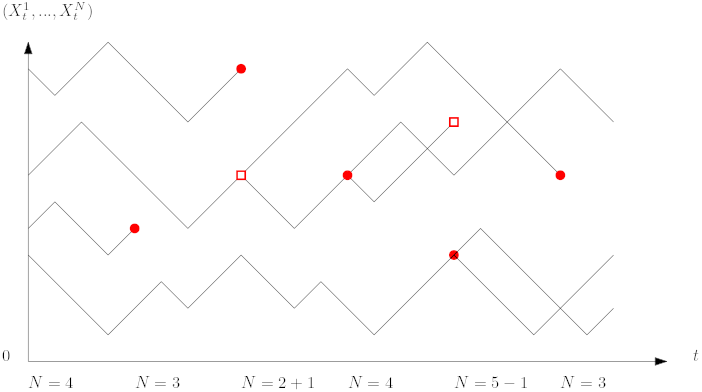
Figure 1: A schematic representation of the $\displaystyle N_{min}-N_{max}$ dynamic with $\displaystyle N_{min}=3$ and $\displaystyle N_{max}=4$. The process starts with $\displaystyle N=4$ particles at time $\displaystyle 0$. The first event is a killing, so that the number of particles goes down to $\displaystyle N=3=N_{min}$. The next event is a killing, so that the number of particles goes down to $\displaystyle 2<N_{min}$, which triggers a resampling event: one of the $\displaystyle 2$ remaining particles (chosen uniformly at random) is duplicated, and the number of particles goes back to $\displaystyle N=2+1=N_{min}$. The next event is a branching, so that the number of particles goes up to $\displaystyle N=4=N_{max}$. The subsequent event is a branching event, so that the number of particles goes up to $\displaystyle 5>N_{max}$, which triggers a selection event, so that one of the $\displaystyle 5$ particles (chosen uniformly at random) is removed from the system, and the number of particles goes back to $\displaystyle N=4=N_{max}$. The next event is a killing, so that the number of particles goes down to $\displaystyle 3=N_{min}$, and so on.

As discussed in [8], the above model and the associated results given in [8] are related to a whole suite of other models in the literature. For example, when $\displaystyle N_{min}=N_{max}$ and $\displaystyle\kappa$ bounded, we recover the standard Moran particle model (see [15, 13, 29, 6] for similar results), where the process is constrained to remain of constant size $\displaystyle N_{0}$.

In addition, our model is reminiscent of the genetic algorithms introduced by Del Moral, see [11, 12] and references therein, and also fits into the more general class of controlled branching processes introduced by Sevastyanov and Zubkov in [30], where the number of reproductive individuals in each generation depends on the size of the previous generation via a control function. We refer the reader to [8] for further discussion and references on these related works.

In the rest of the article we will use the notation

$$m_{t}:=\sum_{i=1}^{N_{t}}\delta_{X_{t}^{i}},\quad t\geq 0,$$

to denote the empirical measure associated with the $\displaystyle N_{min}-N_{max}$ interacting particle system. We will also use $\displaystyle\hat{m}_{t}$ to denote the normalised empirical measure:

$$\hat{m}_{t}:=\frac{1}{N_{t}}\sum_{i=1}^{N_{t}}\delta_{X_{t}^{i}},\quad t\geq 0.$$

The law of the particle system will be denoted by $\displaystyle\mathbb{P}$, with corresponding expectation operator $\displaystyle\mathbb{E}$.

3 Main result

In this section, we present our main result, which improves on the upper bound given in Theorem 1 of [8]. For this, we set

$$h(x)=\inf_{t\geq 1}\frac{\delta_{x}Q_{t}{\mathbf{1}}_{E}}{\|Q_{t-1}{\mathbf{1}}_{E}\|_{\infty}},\ \forall x\in E$$ (3)

and, for all bounded measurable functions $\displaystyle f:E\to\mathbb{R}$,

$$\alpha_{t}(f)=\sup_{x\in E}\left|\frac{\delta_{x}Q_{t}f}{\delta_{x}Q_{t}{\mathbf{1}}_{E}}-\nu_{t}(f)\right|,\ \forall\geq 0,$$ (4)

where $\displaystyle\nu_{t}$ is a (well chosen) probability measure over $\displaystyle E$. We also recall that $\displaystyle Q_{t}$, $\displaystyle m_{t}$ and $\displaystyle\hat{m}_{t}$, $\displaystyle t\geq 0$ were defined in the previous section. We will also use the notation $\displaystyle\mathcal{M}_{1}(E)$ to denote the collection of probability measures on $\displaystyle E$.

Theorem 1.

Under Assumptions 1, 2 and  3, there exists a constant $\displaystyle C>0$ such that, for all $\displaystyle T\geq 1$ and all bounded measurable functions $\displaystyle f:E\to\mathbb{R}$, we have

$$\displaystyle\left\|\frac{\hat{m}_{0}Q_{T}f}{\hat{m}_{0}Q_{T}\mathbf{1}_{E}}-\hat{m}_{T}(f)\right\|_{2} \displaystyle\leq C\sum_{s=0}^{T-1}\alpha_{T-s-1}(f)\mathbb{E}\left(\frac{1}{\sqrt{N_{s}}\hat{m}_{s}(h)}\right).$$ (5)

Remark 2.

After the proof we will consider several examples where $\displaystyle\alpha_{t}$ is bounded by a constant, as well as situations where it decreases exponentially fast with $\displaystyle t$, allowing us to make use of well-known results in the theory of quasi-stationary distribution. In these situations, the right-hand side of (5) is typically linear in $\displaystyle T$ and uniformly bounded over $\displaystyle T\geq 0$ respectively.

However, there are situations where $\displaystyle\alpha_{t}$ may decrease more slowly, for instance in reducible state spaces or in time inhomogeneous settings. Note that these settings are also covered by our result since $\displaystyle\nu_{t}$ is allowed to depend on $\displaystyle t$.

Proof.

We first prove that, for all $\displaystyle\|f\|_{\infty}\leq 1$,

$$\displaystyle\left\|\frac{\hat{m}_{0}Q_{T}f}{\hat{m}_{0}Q_{T}\mathbf{1}_{E}}-\frac{\hat{m}_{1}Q_{T-1}f}{\hat{m}_{1}Q_{T-1}\mathbf{1}_{E}}\right\|_{2}\leq C\frac{\|Q_{T-1}\mathbf{1}_{E}\|_{\infty}\sup_{\mu\in\mathcal{M}_{1}(E)}\left|\frac{\mu Q_{T-1}f}{\mu Q_{T-1}\mathbf{1}_{E}}\right|}{\sqrt{N_{0}}\hat{m}_{0}Q_{T}\mathbf{1}_{E}}.$$ (6)

This is obtained via a modification of the end of the proof of Theorem 2.6 in [8]. Denoting by $\displaystyle A_{t}$ the total number of resampling events up to time $\displaystyle t$, by $\displaystyle B_{t}$ the total number of selection events up to time $\displaystyle t$, and setting

$$\Pi_{t}^{A}\coloneqq\prod_{n=1}^{A_{t}}\left(\frac{N_{min}-1}{N_{min}}\right),\qquad\Pi_{t}^{B}\coloneqq\prod_{i=1}^{B_{t}}\left(\frac{N_{max}+1}{N_{max}}\right),$$ (7)

the authors obtain therein that

$$\mathbb{E}\left[\left(m_{0}Q_{1}f-\Pi_{1}^{A}\Pi_{1}^{B}m_{1}f\right)^{2}\right]\leq c_{1}N_{0}\exp\left(c_{2}\|b\|_{\infty}\right)\left(\sup_{t\in[0,1]}\|Q_{t}f\|_{\infty}\right)^{2},$$

for some constants $\displaystyle c_{1}$ and $\displaystyle c_{2}$. From there, applying this result to $\displaystyle f=Q_{T-1}f$, one deduces that for $\displaystyle T\geq 1$,

$$\displaystyle\left\|m_{0}Q_{T}\mathbf{1}_{E}\,\frac{m_{1}Q_{T-1}f}{m_{1}Q_{T-1}\mathbf{1}_{E}}-m_{0}Q_{T}f\right\|_{2}$$

$$\displaystyle\hskip 56.9055pt\leq\left\|(m_{0}Q_{T}\mathbf{1}_{E}-\Pi_{1}^{A}\Pi_{1}^{B}m_{1}Q_{T-1}\mathbf{1}_{E})\,\frac{m_{1}Q_{T-1}f}{m_{1}Q_{T-1}\mathbf{1}_{E}}\right\|_{2}+\left\|\Pi_{1}^{A}\Pi_{1}^{B}m_{1}Q_{T-1}f-m_{0}Q_{T}f\right\|_{2}$$

$$\displaystyle\hskip 56.9055pt\leq\sqrt{c_{1}N_{0}}\exp\left(c_{2}\|b\|_{\infty}/2\right)\left(\sup_{t\in[0,1]}\|Q_{t+T-1}\mathbf{1}_{E}\|_{\infty}\sup_{\mu\in\mathcal{M}_{1}(E)}\left|\frac{\mu Q_{T-1}f}{\mu Q_{T-1}\mathbf{1}_{E}}\right|+\sup_{t\in[0,1]}\|Q_{t+T-1}f\|_{\infty}\right).$$

We conclude that

$$\left\|\frac{\hat{m}_{0}Q_{T}f}{\hat{m}_{0}Q_{T}\mathbf{1}_{E}}-\frac{\hat{m}_{1}Q_{T-1}f}{\hat{m}_{1}Q_{T-1}\mathbf{1}_{E}}\right\|_{2}\\ \leq C\frac{\sup_{t\in[0,1]}\|Q_{t+T-1}\mathbf{1}_{E}\|_{\infty}\sup_{\mu\in\mathcal{M}_{1}(E)}\left|\frac{\mu Q_{T-1}f}{\mu Q_{T-1}\mathbf{1}_{E}}\right|+\sup_{t\in[0,1]}\|Q_{t+T-1}f\|_{\infty}}{\sqrt{N_{0}}\hat{m}_{0}Q_{T}\mathbf{1}_{E}}.$$

Now note that, for all $\displaystyle\mu\in\mathcal{M}_{1}(E)$,

$$\displaystyle\mu Q_{t+T-1}f\leq\frac{\mu Q_{t+T-1}f}{\mu Q_{t+T-1}\mathbf{1}_{E}}\|Q_{t+T-1}\mathbf{1}_{E}\|_{\infty}$$

Then, since $\displaystyle b$ is assumed bounded, there exists a constant $\displaystyle C>0$ such that

$$\displaystyle\sup_{t\in[0,1]}\|Q_{t+T-1}\mathbf{1}_{E}\|_{\infty}\leq C\|Q_{T-1}\mathbf{1}_{E}\|_{\infty}.$$

Using the last two estimates in the antepenultimate inequality, we deduce that (6) holds true.

Then, using Minkowski’s inequality, the Markov property at each time $\displaystyle s\in\{1,2,\ldots,T-1\}$ and the first step of the proof, we obtain

$$\displaystyle\left\|\frac{\hat{m}_{0}Q_{T}f}{\hat{m}_{0}Q_{T}\mathbf{1}_{E}}-\frac{\hat{m}_{T}(f)}{\hat{m}_{T}(\mathbf{1}_{E})}\right\|_{2} \displaystyle\leq\sum_{s=0}^{T-1}\left\|\frac{\hat{m}_{s}Q_{T-s}f}{\hat{m}_{s}Q_{T-s}\mathbf{1}_{E}}-\frac{\hat{m}_{s+1}Q_{T-s-1}f}{\hat{m}_{s+1}Q_{T-s-1}\mathbf{1}_{E}}\right\|_{2}$$

$$\displaystyle\leq C\sum_{s=0}^{T-1}\mathbb{E}\left(2\wedge\frac{\|Q_{T-s-1}\mathbf{1}_{E}\|_{\infty}\sup_{\mu\in\mathcal{M}_{1}(E)}\left|\frac{\mu Q_{T-s-1}f}{\mu Q_{T-s-1}\mathbf{1}_{E}}\right|}{\sqrt{N_{0}}\hat{m}_{0}Q_{T-s}\mathbf{1}_{E}}\right),$$ (8)

for some constant $\displaystyle C>0$. Replacing $\displaystyle f$ by $\displaystyle f-\nu_{t}(f)$ and using the definitions of $\displaystyle h$ and $\displaystyle\alpha$ yields the result. ∎

Remark 3.

When the function $\displaystyle h$ defined in (3) is bounded away from $\displaystyle 0$, then Theorem 1 entails that there exists a constant $\displaystyle C>0$ such that, for all bounded measurable function $\displaystyle f$ and all time $\displaystyle T>0$,

$$\displaystyle\left\|\frac{\hat{m}_{0}Q_{T}f}{\hat{m}_{0}Q_{T}\mathbf{1}_{E}}-\hat{m}_{T}(f)\right\|_{2} \displaystyle\leq C\frac{T}{\sqrt{N_{min}}}\|f\|_{\infty}.$$ (9)

A similar estimate appeared in [12, Proposition 9.5.6], where the particle system evolves in discrete time with a constant number of particle, under the same assumption on $\displaystyle h$ (transposed to discrete time).

If, in addition, $\displaystyle(\alpha_{t}(f))_{t\in\{1,2,\ldots\}}$ is summable, then there exists a constant $\displaystyle C_{f}>0$ such that, for all $\displaystyle T>0$,

$$\displaystyle\left\|\frac{\hat{m}_{0}Q_{T}f}{\hat{m}_{0}Q_{T}\mathbf{1}_{E}}-\hat{m}_{T}(f)\right\|_{2} \displaystyle\leq\frac{C_{f}}{\sqrt{N_{min}}}.$$ (10)

In the rest of this section, we provide examples that illustrate typical situations where this holds true.

Example 1 (Uniform exponential convergence with bounded soft killing rate).

In [5], it has been proved that there exists a probability measure $\displaystyle\nu_{QS}$ on $\displaystyle E$, constants $\displaystyle C>0$ and $\displaystyle\alpha>0$ such that

$$\displaystyle\left\|\frac{\mu Q_{t}}{\mu Q_{t}{\mathbf{1}}_{E}}-\nu_{QS}\right\|_{TV}\leq Ce^{-\alpha t},\ \forall t\geq 0,\ \forall\mu\in\mathcal{M}_{1}(D),$$

if, and only if, there exist constants $\displaystyle c_{1},c_{2},t_{0}>0$ and $\displaystyle\nu\in\mathcal{M}_{1}(D)$ such the two following conditions are satisfied:

$$\displaystyle\text{(A1).}\qquad\frac{\delta_{x}Q_{t_{0}}}{\delta_{x}Q_{t_{0}}{\mathbf{1}}_{E}}\geq c_{1}\,\nu,\ \forall x\in E,$$

$$\displaystyle\text{(A2).}\qquad\inf_{t\geq 0,\,x\in E}\frac{\nu Q_{t}{\mathbf{1}}_{E}}{\delta_{x}Q_{t}{\mathbf{1}}_{E}}\geq c_{2}.$$

If, in addition, $\displaystyle\inf_{x\in E}\delta_{x}Q_{t_{0}}{\mathbf{1}}_{E}>0$, then this implies that $\displaystyle h$ is uniformly bounded from below and that, for all measurable function $\displaystyle f$, we have $\displaystyle\alpha_{t}(f)\leq Ce^{-\alpha t}\|f\|_{\infty}$, so that the uniform convergence (10) holds true with $\displaystyle C_{f}=C\|f\|_{\infty}$.

The conditions (A1) and (A2) are known to hold true in several situations (see e.g. [15, 11, 12, 5]). In addition, they are easily generalised to the time-inhomogeneous setting, in which case the uniform convergence result follows by taking a time dependent measure in the definition of $\displaystyle\alpha$.

In the particular Moran model setting (that is when $\displaystyle N_{min}=N_{max}$), this uniform convergence result was already known (see e.g. [29, 12, 6]) under additional regularity conditions involving the infinitesimal generator and the carré du champs operator associated to $\displaystyle(Q_{t})_{t\geq 0}$. Our contribution is thus that the uniform convergence holds in a more general setting and without these regularity conditions.

Example 2 (Wasserstein distance).

Consider the case where $\displaystyle E$ is endowed with a bounded metric $\displaystyle d$. Assume that $\displaystyle b-\kappa$ is Lipschitz and that the following assumption holds:

• There exist constants $\displaystyle C,\gamma>0$ such that, for all $\displaystyle x,y\in E$ and $\displaystyle t\geq 0$, there exists a Markovian coupling

  $$\mathbb{E}_{(x,y)}[G_{t}d(X_{t}^{x},X_{t}^{y})]\leq C{\rm e}^{\gamma t}d(x,y),$$

  where $\displaystyle G_{t}^{x}={\rm e}^{-\int_{0}^{t}\beta(X_{s}^{x})-\kappa(X_{s}^{x}){\rm d}s}/\mathbb{E}_{x}[{\rm e}^{-\int_{0}^{t}\beta(X_{s}^{x})-\kappa(X_{s}^{x}){\rm d}s}]$ and $\displaystyle X_{t}^{x}$ denotes $\displaystyle X_{t}$ under $\displaystyle\mathbb{P}_{x}$.

Under these assumptions, it was proved in [4] that there exists a probability measure $\displaystyle\nu_{QS}$ such that for all Lipschitz function $\displaystyle f:E\to\mathbb{R}$, we have

$$\displaystyle\left\|\frac{\mu Q_{t}f}{\mu Q_{t}{\mathbf{1}}_{E}}-\nu_{QS}(f)\right\|_{Lip}\leq Ce^{-\alpha t}W_{d}(\mu,\nu_{QS})\|f\|_{Lip},\ \forall t\geq 0,\ \forall\mu\in\mathcal{M}_{1}(D),$$ (11)

where, for $\displaystyle\mu,\nu\in\mathcal{M}_{1}(D)$, $\displaystyle W_{d}(\mu,\nu)=\sup_{\|f\|_{Lip}\leq 1}|\mu(f)-\nu(f)|$.

In addition, the authors show that $\displaystyle h$ is lower bounded in this case. We refer the reader to [4] for example of processes satisfying this condition.

Under these conditions, we thus obtain that, for all bounded measurable function $\displaystyle f$, (9) holds true, and that, for all Lipschitz function $\displaystyle f$, (10) holds true with $\displaystyle C_{f}=C\,\|f\|_{Lip}$. As far as we know, this result is new, even for the simpler Moran Model (i.e. $\displaystyle N_{min}=N_{max}$).

Example 3 (Counter-example to linear convergence when $\displaystyle h=0$ on some subset).

We consider the case where $\displaystyle E=\{a,b\}$, $\displaystyle a\neq b$, $\displaystyle X$ is the constant continuous Markov chain ($\displaystyle X_{t}=X_{0}$ for all $\displaystyle t\geq 0$, almost surely), $\displaystyle\kappa={\mathbf{1}}_{a}+2\,{\mathbf{1}}_{b}$, and $\displaystyle b=0$. For any $\displaystyle N\geq 2$, define the probability measure $\displaystyle\mu_{N}=\frac{1}{N}\delta_{a}+\frac{N-1}{N}\delta_{b}$, so that

$$\frac{\mu_{N}Q_{t}{\mathbf{1}}_{a}}{\mu_{N}Q_{t}{\mathbf{1}}_{E}}=\frac{\frac{1}{N}\,e^{-t}}{\frac{1}{N}\,e^{-t}+\frac{N-1}{N}\,e^{-2t}}.$$

In particular, for $\displaystyle t=2\ln N$,

$$\frac{\mu_{N}Q_{t}{\mathbf{1}}_{a}}{\mu_{N}Q_{t}{\mathbf{1}}_{E}}=\frac{\frac{1}{N^{3}}}{\frac{1}{N^{3}}+\frac{N-1}{N}\,\frac{1}{N^{4}}}\geq\frac{1}{1+\frac{1}{N}}.$$

Now consider the $\displaystyle N_{min}-N_{max}$ model with $\displaystyle N_{0}=N_{min}=N_{max}$, the same parameters $\displaystyle\kappa$ and $\displaystyle b$, and $\displaystyle X^{1}_{0}=a$ and $\displaystyle X^{i}_{0}=b$ for all $\displaystyle i\geq 2$. Then, with probability $\displaystyle 1/3$, during the first event involving $\displaystyle X^{1}$, the particle jumps to $\displaystyle b$ and there are $\displaystyle 0$ particle at $\displaystyle a$, so that $\displaystyle\hat{m}_{t}(a)=0$ after this event. Since this event happens with rate $\displaystyle 3$, we deduce that

$$\mathbb{E}(\hat{m}_{t}(a))\leq e^{-3t}+(1-e^{-3t})\frac{2}{3},$$

and hence, taking again $\displaystyle t=2\ln N$,

$$\mathbb{E}(\hat{m}_{t}(a))\leq\frac{1}{N^{6}}+\left(1-\frac{1}{N^{6}}\right)\frac{2}{3}.$$

This shows that

$$\mathbb{E}\left(\left|\frac{\mu_{N}Q_{t}{\mathbf{1}}_{a}}{\mu_{N}Q_{t}{\mathbf{1}}_{E}}-\hat{m}_{t}(a)\right|^{2}\right)\geq\frac{1}{1+\frac{1}{N}}-\frac{1}{N^{6}}+(1-\frac{1}{N^{6}})\frac{2}{3}\xrightarrow[N\to+\infty]{}\frac{1}{3},$$

and hence that (9) does not hold true in this setting.

Example 4 (Counter-example to uniform when no uniform convergence of semi-group).

We consider as in the previous example the case where $\displaystyle E=\{a,b\}$, $\displaystyle a\neq b$, and $\displaystyle X$ is the constant continuous time Markov chain ($\displaystyle X_{t}=X_{0}$ for all $\displaystyle t\geq 0$ almost surely), but with $\displaystyle\kappa={\mathbf{1}}_{a}+{\mathbf{1}}_{b}$, and $\displaystyle b=0$. In this case, for any even number $\displaystyle N\geq 2$, we define the probability measure $\displaystyle\mu_{N}=\frac{1}{2}\delta_{a}+\frac{1}{2}\delta_{b}$, so that

$$\frac{\mu_{N}Q_{t}{\mathbf{1}}_{a}}{\mu_{N}Q_{t}{\mathbf{1}}_{E}}=\frac{1}{2}.$$

Now consider the $\displaystyle N_{min}-N_{max}$ model with $\displaystyle N_{0}=N_{min}=N_{max}=N$, the same parameters $\displaystyle\kappa$ and $\displaystyle b$, and $\displaystyle X^{i}_{0}=a$ for all $\displaystyle i\leq N/2$ and $\displaystyle X^{i}_{0}=b$ for all $\displaystyle i\geq N/2+1$. Since the two sets do not communicate with each other, we deduce that there exists $\displaystyle T_{N}\geq 0$ such that $\displaystyle\mathbb{P}(\hat{m}_{T_{N}}(a)=0)\geq 1/4$. We thus deduce that

$$\displaystyle\mathbb{E}\left(\left|\frac{\mu_{N}Q_{T_{N}}{\mathbf{1}}_{a}}{\mu_{N}Q_{T_{N}}{\mathbf{1}}_{E}}-\hat{m}_{T_{N}}(a)\right|^{2}\right)\geq\frac{1}{4}.$$

This shows that, even though $\displaystyle\inf_{E}h>0$, (10) does not hold true.

4 Brownian motion with drift on a bounded $\displaystyle C^{2}$ domain.

In the previous section, we applied our main result to situations where $\displaystyle h$ was uniformly bounded from below. In this section, we consider the more challenging case of a Brownian motion with drift, killed at the boundary of a $\displaystyle C^{2}$-domain. The Fleming-Viot-type particle system with this dynamic has been studied: it is known that, in this case, the empirical distribution converges uniformly in time toward the associated Feynman-Kac semigroup (see e.g. [16], and [24] when the diffusion parameter is sufficiently small) at rate $\displaystyle C/N^{\eta}$ for some $\displaystyle\eta\in(0,1/2)$. The purpose of this section is two-fold: to prove that the $\displaystyle L^{2}$ distance can be (optimally) bounded by $\displaystyle C/\sqrt{N_{min}}$, and to extend the uniform convergence obtained in the Fleming-Viot setting to the more general framework of the $\displaystyle N_{min}-N_{max}$ particle system.

We consider the situation where $\displaystyle X$ is a solution to the SDE

$$dX_{t}=dW_{t}+q(X_{t})\,\mathrm{d}t,\ X_{0}\in D,$$

where $\displaystyle D$ is a bounded domain in $\displaystyle\mathbb{R}^{d}$, $\displaystyle d\geq 2$, with $\displaystyle C^{2}$ boundary, $\displaystyle W$ is a standard $\displaystyle d$-dimensional Brownian motion, and $\displaystyle q:D\to\mathbb{R}^{d}$ is bounded and continuous. We assume that $\displaystyle b$ and $\displaystyle\kappa$ are bounded and that the process is killed upon hitting the boundary at time $\displaystyle\tau_{\partial}=\inf\{t\geq 0,\,X_{t}\notin D\}$.

Theorem 4.

Assumptions 1, 2 and 3 hold true. In addition, there exists a constant $\displaystyle C>0$ such that, for all bounded measurable functions $\displaystyle f:D\to\mathbb{R}$,

$$\displaystyle\left\|\frac{\hat{m}_{0}Q_{T}f}{\hat{m}_{0}Q_{T}\mathbf{1}_{E}}-\hat{m}_{T}(f)\right\|_{2} \displaystyle\leq\frac{C\sqrt{N_{max}}}{N_{min}}\|f\|_{\infty}+\mathbb{E}\left(\frac{C}{\sqrt{N_{0}}\,\hat{m}_{0}(\rho_{D})}\right)\|f\|_{\infty},\ \forall t\geq 0,$$ (12)

where $\displaystyle\rho_{D}:D\to\mathbb{R}_{+}$ denotes the distance to the boundary of $\displaystyle D$.

Proof.

Thanks to equation (3.6) and (A1–A2) of [3] (see also Remark 3 therein), there exists a constant $\displaystyle c_{0}>0$ such that for all $\displaystyle t\geq 1$ and $\displaystyle x\in D$,

$$\displaystyle\frac{\delta_{x}Q_{t}{\mathbf{1}}_{D}}{\sup_{y\in D}\delta_{y}Q_{t-1}{\mathbf{1}}_{D}}\geq c_{0}\rho_{D}(x),$$

where $\displaystyle\rho_{D}$ is the distance to the boundary of $\displaystyle D$. This implies that, for all $\displaystyle t\geq 0$,

$$\mathbb{E}\left(\frac{1}{\sqrt{N_{t}}\hat{m}_{t}(h)}\right)\leq\mathbb{E}\left(\frac{C\sqrt{N_{t}}}{\sum_{i=1}^{N_{t}}\rho_{D}(X^{i}_{t})}\right)\leq\mathbb{E}\left(\frac{C\sqrt{N_{max}}}{\sum_{i=1}^{N_{t}}\rho_{D}(X^{i}_{t})}\right).$$ (13)

It is known that the distance to the boundary for the Fleming-Viot-type system can be stochastically coupled with a system of Brownian motions with drift on $\displaystyle[0,a]$ for some $\displaystyle a>0$, reflected at $\displaystyle 0$ and $\displaystyle a$ (see e.g. [31]). From this coupling for the Fleming-Viot particle system, we derive a new coupling for the $\displaystyle N_{min}-N_{max}$ model.

More precisely, let $\displaystyle a>0$ and $\displaystyle D_{a}=\{x\in D,\ \rho_{D}(x)\leq a\}$ such that the distance to the boundary is $\displaystyle C^{2}$ in $\displaystyle D_{a}$ (such a vicinity of the boundary exists since the boundary is assumed to be of regularity $\displaystyle C^{2}$). Then, when a particle $\displaystyle X^{i}$ is in $\displaystyle D_{a}$, using the fact that $\displaystyle\|\nabla\rho_{D}\|_{2}=1$, Itô’s formula yields

$$\displaystyle\mathrm{d}\rho_{D}(X^{i}_{t})=\mathrm{d}B^{i}_{t}+r(X^{i}_{t})\,\mathrm{d}t,\ i\in\{1,\dots,N_{t}\},$$ (14)

for some independent Brownian motions $\displaystyle B^{i}$, $\displaystyle i=1,\dots,N_{t}$, and some bounded continuous function $\displaystyle r$, up to the next branching or selection or killing or resampling event.

We now construct a family of jumping reflected Brownian motions with drift on $\displaystyle[0,a]$ in such a way that the sum of the positions of these particles is always bounded above by the sum of the distance between a set of $\displaystyle N_{min}$ particles (in the $\displaystyle N_{min}-N_{max}$ process) and the boundary. The construction of such a process follows similar ideas to those presented in [31] and so we leave the details of the construction to the reader. More precisely, for $\displaystyle i\in\{1,\dots,N_{min}\}$, between events, particles move according to the following dynamics,

$$\displaystyle\mathrm{d}R^{i}_{t}=\mathrm{d}B^{i}_{t}-\|r\|_{\infty}\mathrm{d}t+\mathrm{d}L^{i,0}_{t}-\mathrm{d}L^{i,a}_{t},R^{i}_{0}=0,\ i\in\{1,\ldots,N_{min}\},$$

where $\displaystyle L^{x}$ denotes the local time of $\displaystyle R^{i}$ at $\displaystyle x\in\{0,a\}$, where, for each index $\displaystyle i\in\{1,\dots,N_{min}\}$, $\displaystyle B^{i}$ is the same Brownian motion as in (14), and where the processes jump to $\displaystyle 0$ at rate $\displaystyle\|b\|_{\infty}+\|\kappa\|_{\infty}$ independently from each other. In addition, the $\displaystyle R^{i}$ are required to jump according to the following rules.

• When a particle $\displaystyle X_{t}^{i}$, $\displaystyle i=1,\dots,N_{t}$, branches and does not trigger a selection event, we do nothing (so the set of reflected brownian motion does not branch).

• When a particle branches and triggers a selection event,

  • if the selection event removes a particle associated to a reflected Brownian motion $\displaystyle R^{i}$, $\displaystyle i=1,\dots,N_{min}$, this Brownian motion jumps to $\displaystyle 0$ and is associated to the particle newly created (at the branching event);

  • if the selection event removes a particle which is not associated to a reflected Brownian motion, we do nothing.

• When a particle is killed and there is no resampling,

  • if the particle is not associated to a reflected Brownian motion, we do nothing;

  • if the particle is associated to a reflected Brownian motion, then the Brownian motion jumps to $\displaystyle 0$ and is associated to a new particle, not already associated to a Brownian motion.

• When a particle is killed and triggers a resampling event,

  • if the particle is not associated to a reflected Brownian motion, we do nothing;

  • if the particle is associated to a reflected Brownian motion, then the reflected Brownian motion jumps to $\displaystyle 0$ (this is only relevant for soft killing, since in the case of hard killing the associated reflected Brownian motion is already at $\displaystyle 0$) and is now associated to the newly created particle.

The point of this coupling is that it has the following properties:

$$\displaystyle\sum_{i=1}^{N_{t}}\rho_{D}(X^{i}_{t})\geq\sum_{i=1}^{N_{min}}R^{i}_{t},\ \forall t\geq 0,$$

while the $\displaystyle R^{i}$ are independent (the proof is very similar to the one developed in [31] and we leave the details to the reader).

We first remark that, on the event $\displaystyle\lim_{n\to+\infty}\tau_{n}<+\infty$, the distance to the boundary of the particle system accumulates to $\displaystyle 0$ in finite time, and hence that the set of processes $\displaystyle R^{i}$, $\displaystyle i\in\{1,\ldots,N_{min}\}$ accumulates to $\displaystyle 0$. Since this is not possible (by independence of the processes $\displaystyle R^{i}$), we deduce that Assumption 3 holds true. Assumption 2 also holds true since the hitting time of an elliptic diffusion has no atom. Hence the hypotheses of Theorem 1 are satisfied.

We now make use of the following lemma, proved at the end of this section.

Lemma 5.

We have

$$\displaystyle\mathbb{E}\left(\frac{1}{\sum_{i=1}^{N_{min}}R^{i}_{1}}\right)\leq\frac{C}{N_{min}}.$$

for some constant $\displaystyle C>0$.

Using (6) and since, according to [3], we have $\displaystyle\alpha_{t}(f)\leq Ce^{-\gamma t}$ for some $\displaystyle C,\alpha>0$, we deduce from Theorem 1 that (12) holds true. ∎

Proof of Lemma 5.

Assume without loss of generality that $\displaystyle a=1$. Since the random variables $\displaystyle R^{i}_{1}$ have a bounded density $\displaystyle f_{R}$ with respect to the Lebesgue measure on $\displaystyle[0,a]$ and are independent, we have

$$\displaystyle\mathbb{E}\left(\frac{1}{\sum_{i=1}^{N_{min}}R^{i}_{1}}\right) \displaystyle=\int_{0}^{\infty}\mathcal{L}(t)^{N_{min}}\,\mathrm{d}t,$$

where $\displaystyle\mathcal{L}(t)$ is the Laplace transform of $\displaystyle R^{i}_{1}$, that is

$$\displaystyle\mathcal{L}(t)=\int_{0}^{1}e^{-tx}f_{R}(x)\,\mathrm{d}x.$$

Now note that we have

$$\displaystyle\limsup_{t\to+\infty}t\,\mathcal{L}(t) \displaystyle=\limsup_{t\to+\infty}\int_{0}^{1}t\,e^{-tx}f_{R}(x)\,\mathrm{d}x\leq\sup_{[0,1]}f_{R}\,\lim_{t\to+\infty}\int_{0}^{1}t\,e^{-tx}\,\mathrm{d}x=\sup_{[0,1]}f_{R}.$$

Hence there exist constants $\displaystyle c_{\infty},t_{\infty}>0$ such that, for all $\displaystyle t\geq t_{\infty}$,

$$\displaystyle\mathcal{L}(t)\leq\frac{1}{1+c_{\infty}t}.$$

In addition, the derivative of $\displaystyle\mathcal{L}(t)$ is given by

$$\displaystyle\mathcal{L}^{\prime}(t)=-\int_{0}^{1}x\,e^{-tx}f_{R}(x)\,\mathrm{d}x,$$

which is bounded away from $\displaystyle 0$ on compact intervals and hence, for any $\displaystyle t_{0}>0$, there exists a constant $\displaystyle c_{0}>0$ such that, for all $\displaystyle t\in[0,t_{0}]$,

$$\displaystyle\mathcal{L}(t)\leq\frac{1}{1+c_{0}t}.$$

We deduce that there exists $\displaystyle c>0$ such that, for all $\displaystyle t\geq 0$,

$$\displaystyle\mathcal{L}(t)\leq\frac{1}{1+ct}.$$

In particular,

$$\displaystyle\mathbb{E}\left(\frac{1}{\sum_{i=1}^{N_{min}}R^{i}_{1}}\right) \displaystyle\leq\int_{0}^{\infty}\left(\frac{1}{1+ct}\right)^{N_{min}}\,\mathrm{d}t=\frac{1}{c(N_{min}+1)}.$$

∎

References

- [1] J. Bertoin. On a Feynman-Kac approach to growth-fragmentation semigroups and their asymptotic behaviors. Journal of Functional Analysis, 277(11):108270, 2019.
- [2] J. Bertoin et al. Markovian growth-fragmentation processes. Bernoulli, 23(2):1082–1101, 2017.
- [3] N. Champagnat, K. A. Coulibaly-Pasquier, and D. Villemonais. Criteria for Exponential Convergence to Quasi-Stationary Distributions and Applications to Multi-Dimensional Diffusions, pages 165–182. Springer International Publishing, 2018.
- [4] N. Champagnat, E. Strickler, and D. Villemonais. Uniform wasserstein convergence of penalized markov processes. arXiv preprint arXiv:2306.16051, 2023.
- [5] N. Champagnat and D. Villemonais. Exponential convergence to quasi-stationary distribution and Q-process. Probab. Theory Related Fields, 164(1):243–283, 2016.
- [6] B. Cloez and J. Corujo. Uniform in time propagation of chaos for a Moran model. arXiv e-prints, page arXiv:2107.10794, July 2021.
- [7] A. M. Cox, S. C. Harris, E. L. Horton, and A. E. Kyprianou. Multi-species neutron transport equation. Journal of Statistical Physics, 176(2):425–455, 2019.
- [8] A. M. Cox, E. Horton, and D. Villemonais. Binary branching processes with Moran type interactions. Annales de l’Institut Henri Poincare, Probabilites et Statistiques, 2024.
- [9] A. M. G. Cox, E. Horton, and D. Villemonais. Binary branching processes with Moran type interactions: a formal construction of the particle system. Preprint, 2022.
- [10] D. A. Dawson. Measure-valued Markov processes. In École d’Été de Probabilités de Saint-Flour XXI—1991, volume 1541 of Lecture Notes in Math., pages 1–260. Springer, Berlin, 1993.
- [11] P. Del Moral. Feynman-Kac formulae. Probability and its Applications (New York). Springer-Verlag, New York, 2004. Genealogical and interacting particle systems with applications.
- [12] P. Del Moral. Mean field simulation for Monte Carlo integration, volume 126 of Monographs on Statistics and Applied Probability. CRC Press, Boca Raton, FL, 2013.
- [13] P. Del Moral and L. Miclo. Branching and interacting particle systems approximations of Feynman-Kac formulae with applications to non-linear filtering. Springer, 2000.
- [14] P. Del Moral and L. Miclo. A Moran particle system approximation of Feynman–Kac formulae. Stochastic processes and their applications, 86(2):193–216, 2000.
- [15] P. Del Moral and L. Miclo. On the stability of nonlinear Feynman-Kac semigroups. Ann. Fac. Sci. Toulouse Math. (6), 11(2):135–175, 2002.
- [16] P. Del Moral and D. Villemonais. Exponential mixing properties for time inhomogeneous diffusion processes with killing. Bernoulli, 2018.
- [17] A. Etheridge. Some Mathematical Models from Population Genetics: École D’Été de Probabilités de Saint-Flour XXXIX-2009, volume 2012. Springer Science & Business Media, 2011.
- [18] S. C. Harris and M. I. Roberts. The many-to-few lemma and multiple spines. In Annales de l’Institut Henri Poincaré, Probabilités et Statistiques, volume 53, pages 226–242. Institut Henri Poincaré, 2017.
- [19] N. Ikeda, M. Nagasawa, S. Watanabe, et al. Branching Markov processes I. Journal of Mathematics of Kyoto University, 8(2):233–278, 1968.
- [20] N. Ikeda, M. Nagasawa, S. Watanabe, et al. Branching Markov processes II. Journal of Mathematics of Kyoto University, 8(3):365–410, 1968.
- [21] N. Ikeda, M. Nagasawa, S. Watanabe, et al. Branching Markov processes III. Journal of Mathematics of Kyoto University, 9(1):95–160, 1969.
- [22] P. Jagers. General branching processes as Markov fields. Stochastic Processes and their Applications, 32(2):183–212, 1989.
- [23] P. Jagers. Branching processes as population dynamics. Bernoulli, 1(1-2):191–200, 1995.
- [24] L. Journel and P. Monmarché. Uniform convergence of the Fleming-Viot process in a hard killing metastable case. arXiv preprint arXiv:2207.02030, 2022.
- [25] L. Journel and M. Rousset. The particle approximation of quasi-stationary distributions. part˜ i: concentration bounds in the uniform case. arXiv preprint arXiv:2412.15820, 2024.
- [26] A. Lambert. The branching process with logistic growth. Ann. Appl. Probab., 15(2):1506–1535, 2005.
- [27] J. M. Marshall. A branching process for the early spread of a transposable element in a diploid population. Journal of Mathematical Biology, 57(6):811, 2008.
- [28] P. A. P. Moran. Random processes in genetics. In Mathematical proceedings of the cambridge philosophical society, volume 54, pages 60–71. Cambridge University Press, 1958.
- [29] M. Rousset. On the control of an interacting particle estimation of Schrödinger ground states. SIAM J. Math. Anal., 38(3):824–844 (electronic), 2006.
- [30] B. A. Sevastyanov and A. M. Zubkov. Controlled branching processes. Theory of Probability & Its Applications, 19(1):14–24, 1974.
- [31] D. Villemonais. Interacting particle systems and Yaglom limit approximation of diffusions with unbounded drift. Electronic Journal of Probability, 16:1663–1692, 2011.
- [32] D. Villemonais. General approximation method for the distribution of Markov processes conditioned not to be killed. ESAIM Probab. Stat., 18:441–467, 2014.
- [33] N. M. Yanev. Branching processes in cell proliferation kinetics. In Workshop on Branching Processes and Their Applications, pages 159–178. Springer, 2010.