Joint Design and Pricing of Extended Warranties for Multiple Automobiles with Different Price Bands

Abstract

Extended warranties (EWs) are significant source of revenue for capital-intensive products like automobiles. Such products consist of multiple subsystems, providing flexibility in EW customization, for example, bundling a tailored set of subsystems in an EW contract. This, in turn, enables the creation of a service menu with different EW contract options. From the perspective of a third-party EW provider servicing a fleet of automobile brands, we develop a novel model to jointly optimize the design and pricing of EWs in order to maximize the profit. Specifically, the problem is to determine which contracts should be included in the EW menu and identify the appropriate price for each contract. As the complexity of the joint optimization problem increases exponentially with the number of subsystems, two solution approaches are devised to solve the problem. The first approach is based on a mixed-integer second-order cone programming reformulation, which guarantees optimality but is applicable only for a small number of subsystems. The second approach utilizes a two-step iteration process, offering enhanced computational efficiency in scenarios with a large number of subsystems. Through numerical experiments, the effectiveness of our model is validated, particularly in scenarios characterized by high failure rates and a large number of subsystems.

Keywords: Extended warranty; Flexible warranty design; Bundle pricing; Second-order cone programming

1 Introduction

An extended warranty (EW) provides prolonged protection against product failures beyond the manufacturer’s base warranty, which is important for capital-intensive products. Under an EW contract, the provider promises to investigate, assess, and provide compensation if any failure covered in the contract occurs during the extended warranty period (Murthy and Jack, 2014). Unlike base warranties that are an integrated part of product sales and free of charge to customers, EWs have to be bought separately with extra premiums, thus becoming an essential revenue source for providers. Recent years have witnessed substantial growth in the EW market. According to Bias et al. (2024), the global EW market was valued at over $129 billion in the year 2022 and is expected to reach $286 billion by 2032. Among different types of products covered by EW services in the after-sales market, automobiles are particularly prominent due to their high values and extended lifespans. In general, manufacturers provide a base warranty for customers upon automobile delivery, covering a limited use time (e.g., 3 years) and mileage (e.g., 60,000 km). However, the practical service life and mileage of most automobiles exceed those specified in the base warranty, leaving the automobiles unprotected after the base warranty expires. In view of this business opportunity, many EW providers start to offer EW contracts to satisfy customers’ demand of post-warranty protection against automobile failures.

Unlike base warranties regulated by relevant policies, EWs offer greater flexibility in terms of design and pricing, allowing providers to offer more personalized EW contracts. For instance, an EW is allowed to cover a partial set of subsystems in a product, whereas a base warranty generally covers all critical systems as required by most regulation policies. In this sense, a provider can design multiple EW options by bundling different sets of subsystems. As an example, the automobile manufacturer Ford offers four EW options, including PowertrainCARE, BaseCARE, ExtraCARE, and PremiumCARE, which cover 29, 84, 113, and 1000+ components, respectively. However, not all original manufacturers in the market, like Ford, offer EW services to their customers. Consequently, third-party EW providers have emerged to fill this gap to service automobiles produced by different manufacturers and of different functionalities or price bands. For example, Lizhen Company, a leading third-party automobile warranty service provider in China, prescribes the composition of subsystems in their EW contracts based on the power source and the status of base warranty. Specifically, the company roughly categorizes automobiles into three series and offers the corresponding EWs: (1) automobiles under base warranties (T1-T3 series) are offered EW coverage for fixed 16 or 17 major subsystems; (2) automobiles with expired base warranties (T4T5 series) are offered EW coverage for fixed 3 or 4 core subsystems and (3) new energy series are offered EW coverage only for essential electrical systems; see Figure 1 for details. However, this strategy provides the same bundle of subsystems for all automobiles in the same series, with the warranty price depending solely on the automobiles’ price bands, failing to capture the diversity and heterogeneity of subsystems among different automobiles in EW design and pricing.

Figure 1: Current EWs in the after-sales market

In the literature, extensive research efforts have been devoted to the design and pricing of flexible EW menus (Ye et al., 2013; Xie et al., 2017; Wang et al., 2020; Wang, 2023), particularly emphasizing how to specify protection periods for different warranty options and how to price them accordingly. Though such research efforts have significantly contributed to maximizing profits or minimizing costs for EW providers, two main limitations still exist.

First, they typically concentrate on a single automobile brand from a manufacturer’s perspective, which cannot be directly applied to a third-party EW provider. Due to the extensive range of automobile brands and models that third-party providers must service, designing personalized services for each automobile would substantially increase marketing and promotion costs. Second, the EW options in most studies differ only in their protection lengths and prices, but are homogeneous in terms of coverage—that is, the number of systems or services covered (see, e.g., Wang and Ye, 2021; Wang, 2023; Dai et al., 2025). This design does not fully reflect the flexibility of EWs, as it overlooks the difference among various subsystems. To address these two limitations, we categorize automobiles into different groups based on their price bands (e.g., luxury, commercial, and economy) following Chen et al. (2009), thereby simplifying the types of automobiles and reducing promotion costs. Then, we provide a menu of EW contracts consisting of different subsystems for each group of automobiles.

To address the aforementioned issues, we develop a novel methodology to jointly optimize EW contracts from a third-party provider’s perspective. The basic attraction model is adopted to describe customers’ choice probabilities. A bundle pricing approach is used to determine optimal prices for EW contracts covering different numbers of subsystems. Our main focus is on identifying which subsystems should be included in an EW contract, determining the most suitable contracts in the EW menu for each price band of automobiles, and specifying an optimal EW price when bundling different subsystems within each contract. Unfortunately, when fully considering these factors, the joint optimization problem becomes complex due to the following reasons. First, the potential combinations of subsystems in EW contracts grow exponentially as the number of systems increases. Even though the number of contracts in the EW menu for each customer is limited (usually 2 to 5), the specification of optimal compositions for the contracts is still not an easy task. Second, the warranty price is another critical decision variable that affects customers’ utility and the provider’s total profit; jointly optimizing the compositions and prices of EW contracts further increases the difficulty of problem-solving. Finally, the diversity of customers who own automobiles in different price bands leads to variations in their willingness to pay, adding another complication to the optimization process.

In summary, the main contributions of our work include: (1) To the best of our knowledge, this work is the first attempt to jointly optimize the compositions and prices of EW contracts, which is of particular interest to third-party EW providers. (2) We theoretically show that the joint optimization problem is NP-hard. As the complexity of this problem increases exponentially with the number of systems, we propose two solution methods: a mixed-integer second-order cone programming (MISOCP) reformulation method that can ensure optimality but only works for small-scale problems, and a two-step iterative method that can enhance efficiency for large-scale problems. (3) We conduct extensive numerical experiments to verify the proposed two solution approaches. Additionally, we demonstrate the advantages of the joint optimization model over other benchmark models currently used in practice. The impacts of different model parameters on the optimal results and the corresponding managerial insights are also analyzed.

The remainder of this article is organized as follows. Section 2 reviews related literature. Section 3 presents the proposed EW design and pricing model for different automobiles. Section 4 proposes two approaches to solving the joint optimization model. Section 5 presents numerical results for model comparisons and sensitivity analysis. The corresponding management insights are also discussed. Section 6 summarizes the work and points out some future research topics. All proofs and some technical details can be found in Appendix.

2 Literature Review

Warranty services play a significant role in the aftermarket, and the existing literature has paid significant attention to warranty strategy design. Different maintenance strategies such as minimal repair (e.g., Xie and Liao, 2013; Xie et al., 2017), replacement (e.g., Yeh et al., 2005; Park et al., 2016; Liu and Wang, 2023), and preventive maintenance (e.g., Darghouth et al., 2017; Wang et al., 2020; Wu, 2024) have been widely adopted in the base warranty related research. These strategies have also been applied in EW contract design. For example, Su and Shen (2012) studied extended warranty policies under different repair options (namely, minimal, imperfect, and complete) from the manufacturer’s perspective. Li et al. (2023) designed an EW contract for deteriorating products with maintenance duration commitments aiming to maximize manufacturers’ profits. In our work, the replacement strategy is implemented to handle failure claims over the EW period.

Our work builds upon the existing literature on the design and pricing of EW contracts. Hartman and Laksana (2009) proposed a flexible warranty menu for customers, computed their individual optimal choice using dynamic programming, and priced the EW service for each customer. Liu et al. (2020) proposed a flexible post-purchase warranty choice of online registration for customers and optimized the warranty price with heterogeneous customers’ risk attitudes. Wang et al. (2020) and Dai et al. (2025) studied the design and pricing of EW menus under the basic attraction model. In addition, two-dimensional EW services related to the age and mileage of automobiles have been widely discussed in the literature. Wang and Ye (2021) designed a customized EW according to heterogeneous customer usage rates, in which a customer is allowed to choose the age limit of EW based on his/her willingness to pay. Tong et al. (2014) and Wang (2023) focused on two-dimensional EW design based on repair and maintenance services, respectively, and then determined an optimal pricing policy for commercial vehicles. Mitra (2021) focused on optimizing the age and usage limits for a two-dimensional EW incorporating consumer preferences. The existing EW pricing studies focus predominantly on specifying optimal protection lengths and/or prices for EW contracts, provided that the contracts have a homogeneous composition of subsystems. Our work differs from the existing research in the sense that our aim is to seek the optimal compositions and prices for EW contracts under a given protection length.

Furthermore, our paper is also related to the bundle pricing literature. This stream of research can be traced back to the 1960s, when early studies demonstrated that bundling could significantly capture consumer surplus, reduce sales costs, and minimize consumer heterogeneity, thereby playing a crucial role in increasing profits (Stigler, 1963; Adams and Yellen, 1976; Schmalensee, 1984). Guiltinan (1987) proposed a bundle pricing strategy of two or more products or services at a special discount, which extended the economic theory of bundling to encompass various types of complementary relationships. Hanson and Martin (1990) did one of the important prior works to consider multiple components and obtain the optimal bundling prices by mixed integer programming. Bitran and Ferrer (2007) addressed a problem of determining the optimal composition and price for high-tech manufacturers by separating the two decisions: optimizing price through derivative analysis and optimizing composition based on a revenue-by-order criterion. Thereafter, bundle pricing strategies have been widely investigated for complementary products (Giri et al., 2020; Taleizadeh et al., 2020) and competitive products (Lin et al., 2020). Some recent research also considered other important factors such as customers’ behaviors. For example, Nie et al. (2024) discussed the advantages of bundle and add-on sales strategies using game theory considering customer returns in e-commerce. In addition to traditional applications in manufacturing and retail industries, bundle pricing also found its application potential in healthcare management. Proano et al. (2012) focused on how to combine and price different types of vaccines to satisfy the demand of low-income countries. However, the bundle pricing strategy has not yet been applied to EWs for multiple subsystems in automobiles. We contribute to the literature by personalizing the compositions—in terms of subsystems—of EW contracts for multiple automobiles with different price bands, and by implementing optimized bundle pricing strategies to maximize the third-party EW provider’s profit.

3 Joint Optimization Model

In this section, a joint optimization model is developed for the design and pricing of EW contracts for multiple automobiles. Section 3.1 first describes the basic model setting. Section 3.2 then presents a joint optimization model for EW design and pricing from the perspective of a third-party warranty provider. The notation used throughout this paper is summarized in Appendix A.

3.1 Model Setting

In this paper, automobiles are grouped into $m$ price bands such as luxury, commercial, and economy, indexed by $j\in\mathcal{M}:=\{1,2,\dots,m\}$. A customer who owns an automobile in the $j$th group is correspondingly defined as a group-$j$ customer. The proportion of group-$j$ customers is defined as $\lambda_{j}$, with $\sum_{j\in\mathcal{M}}\lambda_{j}=1$. Suppose that there are $w$ subsystems (e.g., engine systems, suspension systems), indexed by $k\in\mathcal{W}:=\{1,2,\dots,w\}$, that are critical to the functioning of automobiles. In total, there are $n=2^{w}-1$ potential system combinations for each contract, which are indexed by $i\in\mathcal{N}:=\{1,2,\dots,n\}$. We use a binary value $\mathbb{I}_{ik}$ to indicate whether system $k$ is included in EW contract $i$. That is, if system $k$ is present in contract $i$, then $\mathbb{I}_{ik}=1$; otherwise, $\mathbb{I}_{ik}=0$. The provider faces a decision on recommending a proper EW contract to each group of customers. To this end, we use the binary variable $x_{ij}$ to indicate whether contract $i$ should be recommended to group-$j$ customers. That is, if contract $i$ is recommended to group-$j$ customers, then $x_{ij}=1$; otherwise, $x_{ij}=0$.

In this work, we consider two cost elements that are incurred to the provider when managing the EW business: warranty cost for servicing customer claims and advertising cost for promoting EWs. We adopt the replacement policy to handle failure claims; that is, the EW provider is obligated to replace the failed systems with new identical ones free of charge to customers. Let $f_{kj}$ represent the failure probability of system $k$ in group-$j$ automobiles over the EW period, and $c_{kj}$ the associated replacement cost. Moreover, since the provider can consolidate the advertising activity for contracts designed for different groups of automobiles as long as the contracts cover the same system combination, we use a binary variable $y_{i}$ to denote whether contract $i$ should be advertised (namely, included in the displayed menu, as shown in Fig. 1). That is, as long as contract $i$ is recommended for any automobile in group $j$ (i.e., $\exists$ $j\in\mathcal{M}$ $|$ $x_{ij}=1$), $y_{i}$ should be set to 1, and the marginal advertising cost $\theta$ should be incurred to the EW provider.

In our context, an EW contract is usually composed of multiple subsystems. As a result, the warranty price should be dependent on the protected subsystems and the price band of the automobiles. Let $p_{ij}$ be the price of EW contract $i$ for automobiles in group $j$. The pricing mechanism is as follows. For each group $j$, an initial price $P_{kj}^{0}$ is predefined for each system $k$, which is proportional to the corresponding failure cost $c_{kj}$. Then, we adopt the pricing strategy proposed by Guiltinan (1987), which is a normative framework for optimizing the different mixed-bundling discounts for the different systems it includes. Compared to an equivalent price promotion strategy, the bundle discount-based strategy shows advantages in attracting consumers (Janiszewski and Cunha Jr, 2004) and enhancing their loyalty in a competitive market (Balachander et al., 2010). In line with the discrete price ladder practice (Cohen et al., 2021), the bundle discount is usually restricted to a finite set of admissible values, defined as ${d_{\mathcal{L}}}=\{d_{1},d_{2},\dots,d_{l}\}$. Without loss of generality, we assume that the discounts are indexed such that

$$d_{1}>d_{2}>\dots>d_{l},$$

where a smaller value of $d_{h}$ ($h\in\mathcal{L}:=\{1,2,\dots,l\}$) indicates a larger discount. We use the binary variable $z_{ih}$ to indicate whether discount level $d_{h}$ should be assigned to contract $i$. If discount $d_{h}$ is selected for contract $i$, then $z_{ih}=1$; otherwise, $z_{ih}=0$. In this manner, the final price of EW contract $i$ shown to group-$j$ customers is expressed as

$$p_{ij}=\left(\sum_{k\in\mathcal{W}}\mathbb{I}_{ik}P_{kj}^{0}\right)\left(\sum_{h\in\mathcal{L}}z_{ih}d_{h}\right),$$ (1)

with $\sum_{h\in\mathcal{L}}z_{ih}=1$, meaning that only one discount level can be assigned to each contract $i$.

Suppose that customers are rational in the sense that they make their purchase choices to maximize their utilities. Let $u_{ij}$ denote the net utility of EW contract $i$ for group-$j$ customers, which is related to the valuation and price of the contract. The average valuation depends on the subsystems covered by the contract. Let $v_{kj}$ represent the average valuation of the protection for system $k$ perceived by a group-$j$ customer. If the valuations of the protections for different subsystems are assumed to be additive, then the valuation of contract $i$ perceived by a group-$j$ customer can be evaluated by $\sum_{k\in\mathcal{W}}\mathbb{I}_{ik}v_{kj}$. Further let $\beta_{j}>0$ denote the price sensitivity of group-$j$ customers. Then, the utility $u_{ij}$ can be denoted as

$$u_{ij}=\sum_{k\in\mathcal{W}}\mathbb{I}_{ik}v_{kj}-\beta_{j}p_{ij}.$$ (2)

Furthermore, let $u_{0j}$ denote the net utility of the no-purchase option for group-$j$ customers.

3.2 Joint EW Design and Pricing Model

Based on the setting described above, we develop a mixed integer programming model to seek optimal compositions and prices of EWs in order to maximize the expected total profit from a third-party EW provider’s perspective.

According to the demand setting in Wang et al. (2020), we employ the basic attraction model to describe customers’ choice among available EW contracts. Based on the customer utility $u_{ij}$ defined in Equation (2), the probability that a group-$j$ customer chooses contract $i$ is given by

$$q_{ij}\left(p_{ij},x_{ij}\right)=\frac{\sum_{k\in\mathcal{W}}\mathbb{I}_{ik}v_{kj}-\beta_{j}p_{ij}}{u_{0j}+\sum_{i\in\mathcal{N}}\left[\sum_{k\in\mathcal{W}}\mathbb{I}_{ik}v_{kj}-\beta_{j}p_{ij}\right]x_{ij}}x_{ij}.$$ (3)

Once a group-$j$ customer chooses an EW contract $i$, the marginal profit for the EW provider can be calculated as the difference between the sales revenue and the warranty cost (i.e., $p_{ij}-\sum_{k\in\mathcal{W}}\mathbb{I}_{ik}f_{kj}c_{kj}$).

Based on the marginal profit and the choice probability of each EW contract, the expected total profit for the EW provider can be evaluated by Equation (4) below. Then, the joint EW design and pricing problem (JDPEW) is defined as

$$\max\quad \sum_{j\in\mathcal{M}}\lambda_{j}\sum_{i\in\mathcal{N}}q_{ij}\left(p_{ij},x_{ij}\right)\left[p_{ij}-\sum_{k\in\mathcal{W}}\mathbb{I}_{ik}f_{kj}c_{kj}\right]-\sum_{i\in\mathcal{N}}\theta y_{i}$$ (4)

s.t. $$x_{ij}\leq y_{i} \forall i\in\mathcal{N},\leavevmode\nobreak\ j\in\mathcal{M}$$ (5)

$$\sum_{i\in\mathcal{N}}\mathbb{I}_{ik}x_{ij}\geq 1\quad \forall k\in\mathcal{W},\leavevmode\nobreak\ j\in\mathcal{M}$$ (6)

$$\sum_{h\in\mathcal{L}}z_{ih}=1 \forall i\in\mathcal{N}$$ (7)

$$\left(\sum_{h\in\mathcal{L}}z_{ih}d_{h}-\sum_{h^{\prime}\in\mathcal{L}}z_{i^{\prime}h^{\prime}}d_{h^{\prime}}\right)\left(\sum_{k\in\mathcal{W}}\mathbb{I}_{ik}-\sum_{k\in\mathcal{W}}\mathbb{I}_{i^{\prime}k}\right)\leq 0 \forall i,\leavevmode\nobreak\ i^{\prime}\in\mathcal{N}$$ (8)

$$p_{ij}=\left(\sum_{k\in\mathcal{W}}\mathbb{I}_{ik}P_{kj}^{0}\right)\left(\sum_{h\in\mathcal{L}}z_{ih}d_{h}\right) \forall i\in\mathcal{N},\leavevmode\nobreak\ j\in\mathcal{M}$$ (9)

$$y_{i}\in\{0,1\},x_{ij}\in\{0,1\},z_{ih}\in\{0,1\},p_{ij}\geq 0 \forall i\in\mathcal{N},\leavevmode\nobreak\ j\in\mathcal{M},\leavevmode\nobreak\ h\in\mathcal{L}.$$ (10)

The objective is to maximize the expected total profit, calculated as the expected revenues minus the warranty servicing and advertising costs for all EWs. Constraint (5) ensures that the recommended EW contracts for each group of automobiles must be advertised to customers. Constraint (6) states that for each group of automobiles, every functional system must appear at least once in the final recommended EWs. In this manner, we guarantee that any system of each group of automobiles can be included in the EW contract to accommodate customers’ specific preferences for particular subsystems. Constraint (7) guarantees that each EW contract has only one price. Constraint (8) indicates that the EW provider offers a larger discount to customers who purchase EWs with a larger number of systems simultaneously so as to stimulate demand. Therefore, the more systems an EW contract includes, the larger discount it has. Constraint (9) represents the bundle pricing mechanism.

We remark that the provider can jointly promote EWs that consist of identical subsystems across multiple groups of automobiles with different price bands so as to reduce advertising costs. The resultant advertising cost $\sum_{i\in\mathcal{N}}\theta y_{i}$ in (4) cannot be decomposed by automobile group $j$. As a result, the optimization problem in (4) cannot be decomposed into several smaller-scale subproblems, each focusing on the EW design and pricing for only one group of automobiles. In essence, the (JDPEW) is a nonlinear program with a large number of decision variables and constraints, which poses significant challenges for problem solving. The following proposition reveals the hardness of this problem.

Proposition 1 (Hardness).

Problem (JDPEW) is NP-hard.

To solve this NP-hard problem, we propose two tractable approaches in the next section.

4 Solution Approaches

In this section, we focus on the solution approaches of Problem (JDPEW), and the optimality and computational complexity are also analyzed. Before proposing the solution, we first substitute Constraint (9) into objective function (4), then define $\hat{V}_{ij}=\sum_{k\in\mathcal{W}}\mathbb{I}_{ik}v_{kj}$, $\hat{P}_{ij}=\sum_{k\in\mathcal{W}}\mathbb{I}_{ik}P^{0}_{kj}$, and $\hat{C}_{ij}=\sum_{k\in\mathcal{W}}\mathbb{I}_{ik}f_{kj}c_{jk}$ to simplify the notations. Based on this reformulation, the objective function in (4) can be rewritten as

$$\max\sum_{j\in\mathcal{M}}\lambda_{j}\frac{\sum_{i\in\mathcal{N}}\left[\hat{V}_{ij}-\beta_{j}\hat{P}_{ij}\left(\sum_{h\in\mathcal{L}}z_{ih}d_{h}\right)\right]\left[\hat{P}_{ij}\left(\sum_{h\in\mathcal{L}}z_{ih}d_{h}\right)-\hat{C}_{ij}\right]x_{ij}}{u_{0j}+\sum_{i\in\mathcal{N}}\left[\hat{V}_{ij}-\beta_{j}\hat{P}_{ij}\left(\sum_{h\in\mathcal{L}}z_{ih}d_{h}\right)\right]x_{ij}}-\sum_{i\in\mathcal{N}}\theta y_{i}.$$ (11)

Based on (11), we propose two solution approaches—that is, MISOCP reformulation and two-step iterations in Sections 4.1 and 4.2, respectively, and analyze their properties.

4.1 Approach 1: MISOCP Reformulation

Letting $\hat{R}_{j}=\max_{i\in\mathcal{N}}\left\{\hat{P}_{ij}-\hat{C}_{ij}\right\}$, the objective (11) can be rewritten as

$$\footnotesize\max\sum_{j\in\mathcal{M}}\lambda_{j}\hat{R}_{j}-\sum_{j\in\mathcal{M}}\lambda_{j}\frac{u_{0j}\hat{R}_{j}+\sum_{i\in\mathcal{N}}\left[\hat{V}_{ij}-\beta_{j}\hat{P}_{ij}\left(\sum_{h\in\mathcal{L}}z_{ih}d_{h}\right)\right]\left[\hat{R}_{j}-\hat{P}_{ij}\left(\sum_{h\in\mathcal{L}}z_{ih}d_{h}\right)+\hat{C}_{ij}\right]x_{ij}}{u_{0j}+\sum_{i\in\mathcal{N}}\left[\hat{V}_{ij}-\beta_{j}\hat{P}_{ij}\left(\sum_{h\in\mathcal{L}}z_{ih}d_{h}\right)\right]x_{ij}}-\sum_{i\in N}\theta y_{i}.$$ (12)

As the term $\sum_{j\in\mathcal{M}}\lambda_{j}\hat{R}_{j}$ is a constant, the profit-maximization problem in (12) is equivalent to the following minimization problem:

$$\footnotesize\min\sum_{j\in\mathcal{M}}\lambda_{j}\frac{u_{0j}\hat{R}_{j}+\sum_{i\in\mathcal{N}}\left[\hat{V}_{ij}-\beta_{j}\hat{P}_{ij}\left(\sum_{h\in\mathcal{L}}z_{ih}d_{h}\right)\right]\left[\hat{R}_{j}-\hat{P}_{ij}\left(\sum_{h\in\mathcal{L}}z_{ih}d_{h}\right)+\hat{C}_{ij}\right]x_{ij}}{u_{0j}+\sum_{i\in\mathcal{N}}\left[\hat{V}_{ij}-\beta_{j}\hat{P}_{ij}\left(\sum_{h\in\mathcal{L}}z_{ih}d_{h}\right)\right]x_{ij}}+\sum_{i\in N}\theta y_{i}.$$ (13)

Let

$$t_{j}=\frac{1}{u_{0j}+\sum_{i\in\mathcal{N}}\left[\hat{V}_{ij}-\beta_{j}\hat{P}_{ij}\left(\sum_{h\in\mathcal{L}}z_{ih}d_{h}\right)\right]x_{ij}}$$

and

$$w_{j}=u_{0j}+\sum_{i\in\mathcal{N}}\left[\hat{V}_{ij}-\beta_{j}\hat{P}_{ij}\left(\sum_{h\in\mathcal{L}}z_{ih}d_{h}\right)\right]x_{ij}.$$

Then, model (JDPEW) can be posed as (JDPEW-1):

$$\min\quad \sum_{j\in\mathcal{M}}\lambda_{j}u_{0j}\hat{R}_{j}t_{j}+\sum_{i\in\mathcal{N}}\theta y_{i}+\sum_{j\in\mathcal{M}}\lambda_{j}\sum_{i\in\mathcal{N}}\left(\hat{V}_{ij}\hat{R}_{j}x_{ij}-\hat{V}_{ij}\hat{P}_{ij}\left(\sum_{h\in\mathcal{L}}z_{ih}x_{ij}d_{h}\right)+\hat{V}_{ij}\hat{C}_{ij}x_{ij}\right)t_{j}+$$

$$\sum_{j\in\mathcal{M}}\lambda_{j}\sum_{i\in\mathcal{N}}\left(-\beta_{j}\hat{R}_{j}\hat{P}_{ij}\left(\sum_{h\in\mathcal{L}}z_{ih}x_{ij}d_{h}\right)+\beta_{j}\hat{P}_{ij}^{2}\left(\sum_{h\in\mathcal{L}}z_{ih}x_{ij}d_{h}^{2}\right)-\beta_{j}\hat{P}_{ij}\left(\sum_{h\in\mathcal{L}}z_{ih}x_{ij}d_{h}\right)\hat{C}_{ij}\right)t_{j}$$ (14)

s.t. $$(\ref{constraint1})-(\ref{constraint6})$$

$$t_{j}w_{j}=1\quad \forall j\in\mathcal{M}\qquad\quad$$ (15)

$$w_{j}=u_{0j}+\sum_{i\in\mathcal{N}}\left[\hat{V}_{ij}x_{ij}-\beta_{j}\hat{P}_{ij}\left(\sum_{h\in\mathcal{L}}z_{ih}x_{ij}d_{h}\right)\right] \forall j\in\mathcal{M}$$ (16)

$$t_{j}\geq 0,w_{j}\geq 0 \forall j\in\mathcal{M}.$$ (17)

Let $s_{ijh}=z_{ih}x_{ij}$. According to McCormick (1976), we can replace constraint $s_{ijh}=z_{ih}x_{ij}$ with the next $4\times m\times n\times l$ constraints:

$$s_{ijh} \geq z_{ih}+\left(x_{ij}-1\right)\quad \forall i\in\mathcal{N},\leavevmode\nobreak\ j\in\mathcal{M},\leavevmode\nobreak\ h\in\mathcal{L}$$ (18)

$$s_{ijh} \geq 0\quad \forall i\in\mathcal{N},\leavevmode\nobreak\ j\in\mathcal{M},\leavevmode\nobreak\ h\in\mathcal{L}$$ (19)

$$s_{ijh} \leq z_{ih}\quad \forall i\in\mathcal{N},\leavevmode\nobreak\ j\in\mathcal{M},\leavevmode\nobreak\ h\in\mathcal{L}\qquad$$ (20)

$$s_{ijh} \leq x_{ij}\quad \forall i\in\mathcal{N},\leavevmode\nobreak\ j\in\mathcal{M},\leavevmode\nobreak\ h\in\mathcal{L}.$$ (21)

Then, model (JDPEW-1) can be posed as (JDPEW-2):

$$\min\quad \sum_{j\in\mathcal{M}}\lambda_{j}u_{0j}\hat{R}_{j}t_{j}+\sum_{i\in\mathcal{N}}\theta y_{i}+\sum_{j\in\mathcal{M}}\lambda_{j}\sum_{i\in\mathcal{N}}\left(\hat{V}_{ij}\hat{R}_{j}x_{ij}-\hat{V}_{ij}\hat{P}_{ij}\left(\sum_{h\in\mathcal{L}}s_{ijh}d_{h}\right)+\hat{V}_{ij}\hat{C}_{ij}x_{ij}\right)t_{j}$$

$$+\sum_{j\in\mathcal{M}}\lambda_{j}\sum_{i\in\mathcal{N}}\left(-\beta_{j}\hat{R}_{j}\hat{P}_{ij}\left(\sum_{h\in\mathcal{L}}s_{ijh}d_{h}\right)+\beta_{j}\hat{P}_{ij}^{2}\left(\sum_{h\in\mathcal{L}}s_{ijh}d_{h}^{2}\right)-\beta_{j}\hat{P}_{ij}\left(\sum_{h\in\mathcal{L}}s_{ijh}d_{h}\right)\hat{C}_{ij}\right)t_{j}$$ (22)

s.t. $$(\ref{constraint1})-(\ref{constraint6}),(\ref{constraint:tw}),\text{and }(\ref{w})-(\ref{s_end})$$

$$w_{j}=u_{0j}+\sum_{i\in\mathcal{N}}\left[\hat{V}_{ij}x_{ij}-\beta_{j}\hat{P}_{ij}\left(\sum_{h\in\mathcal{L}}s_{ijh}d_{h}\right)\right] \forall j\in\mathcal{M}.$$ (23)

Let $g_{ij}=t_{j}x_{ij}$ and $o_{ijh}=\mathrm{s}_{ijh}t_{j}$. Similarly, we can replace these two equalities with constraints (24)-(27) and (28)-(31), respectively, as follows:

$$g_{ij}\geq t_{j}+\left(x_{ij}-1\right)t_{j}^{U}\quad \forall i\in\mathcal{N},\leavevmode\nobreak\ j\in\mathcal{M}$$ (24)

$$g_{ij}\geq x_{ij}t_{j}^{L}\quad \forall i\in\mathcal{N},\leavevmode\nobreak\ j\in\mathcal{M}$$ (25)

$$g_{ij}\leq t_{j}+\left(x_{ij}-1\right)t_{j}^{L}\quad \forall i\in\mathcal{N},\leavevmode\nobreak\ j\in\mathcal{M}$$ (26)

$$g_{ij}\leq x_{ij}t_{j}^{U}\quad \forall i\in\mathcal{N},\leavevmode\nobreak\ j\in\mathcal{M}$$ (27)

$$o_{jih}\geq s_{ijh}t_{j}^{L}\quad \forall i\in\mathcal{N},\leavevmode\nobreak\ j\in\mathcal{M},\leavevmode\nobreak\ h\in\mathcal{L}$$ (28)

$$o_{jih}\geq t_{j}+\left(s_{ijh}-1\right)t_{j}^{U}\quad \forall i\in\mathcal{N},\leavevmode\nobreak\ j\in\mathcal{M},\leavevmode\nobreak\ h\in\mathcal{L}$$ (29)

$$o_{ijh}\leq t_{j}+\left(s_{ijh}-1\right)t_{j}^{L}\quad \forall i\in\mathcal{N},\leavevmode\nobreak\ j\in\mathcal{M},\leavevmode\nobreak\ h\in\mathcal{L}$$ (30)

$$o_{ijh}\leq s_{ijh}t_{j}^{U}\quad \forall i\in\mathcal{N},\leavevmode\nobreak\ j\in\mathcal{M},\leavevmode\nobreak\ h\in\mathcal{L},$$ (31)

where $t_{j}^{L}=1/(u_{0j}+\sum_{i\in\mathcal{N}}\hat{V}_{ij})$ and $t_{j}^{U}=1/u_{0j}$. Observing that $w_{j}\geq 0$, we can state constraint (15) in the rotated cone form:

$$w_{j}t_{j}\geq 1\quad\forall j\in\mathcal{M}.$$ (32)

Finally, we reformulate (JDPEW) as the following model denoted by (JDPEW-MISOCP):

$$\min\quad \sum_{j\in\mathcal{M}}\lambda_{j}u_{0j}\hat{R}_{j}t_{j}+\sum_{i\in\mathcal{N}}\theta y_{i}+\sum_{j\in\mathcal{M}}\lambda_{j}\sum_{i\in\mathcal{N}}\left(\hat{V}_{ij}\hat{R}_{j}g_{ij}-\hat{V}_{ij}\hat{P}_{ij}\left(\sum_{h\in\mathcal{L}}o_{ijh}d_{h}\right)+\hat{V}_{ij}\hat{C}_{ij}g_{ij}\right)+\qquad$$

$$\sum_{j\in\mathcal{M}}\lambda_{j}\sum_{i\in\mathcal{N}}\left(-\beta_{j}\hat{R}_{j}\hat{P}_{ij}\left(\sum_{h\in\mathcal{L}}o_{ijh}d_{h}\right)+\beta_{j}\hat{P}_{ij}^{2}\left(\sum_{h\in\mathcal{L}}o_{ijh}d_{h}^{2}\right)-\beta_{j}\hat{P}_{ij}\left(\sum_{h\in\mathcal{L}}o_{ijh}d_{h}\right)\hat{C}_{ij}\right)$$

s.t. $$x_{ij}\leq y_{i} \forall i\in\mathcal{N},\leavevmode\nobreak\ j\in\mathcal{M}$$

$$\sum_{i\in\mathcal{N}}\mathbb{I}_{ik}x_{ij}\geq 1\quad \forall k\in\mathcal{W},\leavevmode\nobreak\ j\in\mathcal{M}$$

$$\sum_{h\in\mathcal{L}}z_{ih}=1 \forall i\in N$$

$$\left(\sum_{h\in\mathcal{L}}z_{ih}d_{h}-\sum_{h^{\prime}\in L}z_{i^{\prime}h^{\prime}}d_{h^{\prime}}\right)\left(\sum_{k\in\mathcal{W}}\mathbb{I}_{ik}-\sum_{k\in\mathcal{W}}\mathbb{I}_{i^{\prime}k}\right)\leq 0 \forall i,\leavevmode\nobreak\ i^{\prime}\in N$$

$$p_{ij}=\left(\sum_{k\in\mathcal{W}}\mathbb{I}_{ik}P_{kj}^{0}\right)\left(\sum_{h\in\mathcal{L}}z_{ih}d_{h}\right) \forall i\in\mathcal{N},\leavevmode\nobreak\ j\in\mathcal{M}$$

$$w_{j}t_{j}\geq 1\quad \forall j\in\mathcal{M}$$

$$w_{j}=u_{0j}+\sum_{i\in\mathcal{N}}\left[\hat{V}_{ij}x_{ij}-\beta_{j}\hat{P}_{ij}\left(\sum_{h\in\mathcal{L}}s_{ijh}d_{h}\right)\right] \forall j\in\mathcal{M}$$

$$s_{ijh}\geq z_{ih}+\left(x_{ij}-1\right)\quad \forall i\in\mathcal{N},\leavevmode\nobreak\ j\in\mathcal{M},\leavevmode\nobreak\ h\in\mathcal{L}$$

$$s_{ijh}\geq 0\quad \forall i\in\mathcal{N},\leavevmode\nobreak\ j\in\mathcal{M},\leavevmode\nobreak\ h\in\mathcal{L}$$

$$s_{ijh}\leq z_{ih}\quad \forall i\in\mathcal{N},\leavevmode\nobreak\ j\in\mathcal{M},\leavevmode\nobreak\ h\in\mathcal{L}$$

$$s_{ijh}\leq x_{ij}\quad \forall i\in\mathcal{N},\leavevmode\nobreak\ j\in\mathcal{M},\leavevmode\nobreak\ h\in\mathcal{L}$$

$$g_{ij}\geq t_{j}+\left(x_{ij}-1\right)t_{j}^{U}\quad \forall i\in\mathcal{N},\leavevmode\nobreak\ j\in\mathcal{M}$$

$$g_{ij}\geq x_{ij}t_{j}^{L}\quad \forall i\in\mathcal{N},\leavevmode\nobreak\ j\in\mathcal{M}$$

$$g_{ij}\leq t_{j}+\left(x_{ij}-1\right)t_{j}^{L}\quad \forall i\in\mathcal{N},\leavevmode\nobreak\ j\in\mathcal{M}$$

$$g_{ij}\leq x_{ij}t_{j}^{U}\quad \forall i\in\mathcal{N},\leavevmode\nobreak\ j\in\mathcal{M}$$

$$o_{ijh}\geq s_{ijh}t_{j}^{L}\quad \forall i\in\mathcal{N},\leavevmode\nobreak\ j\in\mathcal{M},\leavevmode\nobreak\ h\in\mathcal{L}$$

$$o_{ijh}\geq t_{j}+\left(s_{ijh}-1\right)t_{j}^{U}\quad \forall i\in\mathcal{N},\leavevmode\nobreak\ j\in\mathcal{M},\leavevmode\nobreak\ h\in\mathcal{L}$$

$$o_{ijh}\leq t_{j}+\left(s_{ijh}-1\right)t_{j}^{L}\quad \forall i\in\mathcal{N},\leavevmode\nobreak\ j\in\mathcal{M},\leavevmode\nobreak\ h\in\mathcal{L}$$

$$o_{ijh}\leq s_{ijh}t_{j}^{U}\quad \forall i\in\mathcal{N},\leavevmode\nobreak\ j\in\mathcal{M},\leavevmode\nobreak\ h\in\mathcal{L}$$

$$y_{i}\in\{0,1\},x_{ij}\in\{0,1\},z_{ih}\in\{0,1\},p_{ij}\geq 0\quad \forall i\in\mathcal{N},\leavevmode\nobreak\ j\in\mathcal{M},\leavevmode\nobreak\ h\in\mathcal{L}.$$

After the aforementioned transformation, the original Problem (JDPEW) is simplified as a mixed integer linear programming (JDPEW-MISOCP), which can be solved by Gurobi directly. Indeed, the following proposition confirms that these two problems are equivalent.

Proposition 2.

The optimal solutions $\{x_{ij}^{*},y_{i}^{*},z_{ih}^{*},p^{*}_{ij}\}$ obtained by (JDPEW-MISOCP) are also optimal for (JDPEW).

4.2 Approach 2: Two-step Iterated Approach

Though the MISOCP transformation approach can obtain the optimal solution, it has high computational complexity especially when the number of decision variables and constraints are large. Therefore, as the number of subsystems increases, the computational complexity of Approach 1 grows exponentially, requiring a substantial amount of time to reach the optimal solution.

In this subsection, we propose an alternative approach, named Approach 2, which solves this complex joint optimization problem by a two-step scheme. In the EW design step, subsystems are recommended in EW contracts with a fixed price discount. In the pricing step, the pricing discount is optimized based on the given EW contracts obtained in the design step. These two steps are implemented iteratively until all decision variables are convergent. We detail the sub-optimization problems of these two steps as follows.

Step 1: EW Design. In this step, we focus mainly on the optimization problem to design EW contracts with different subsystems for multiple groups of automobiles from the perspective of EW providers. Given the initial prices of subsystems and discounts, the optimal system recommendation can be obtained based on the following model:

$$\max \sum_{j\in\mathcal{M}}\lambda_{j}\sum_{i\in\mathcal{N}}q_{ij}\left(p_{ij}^{*},x_{ij}\right)\left[p^{*}_{ij}-\sum_{k\in\mathcal{W}}\mathbb{I}_{ik}f_{kj}c_{jk}\right]-\sum_{i\in\mathcal{N}}\theta y_{i}$$

s.t $$x_{ij}\leq y_{i}\hskip 180.00027pt\forall i\in\mathcal{N},\leavevmode\nobreak\ j\in\mathcal{M}$$

$$\sum_{i\in\mathcal{N}}\mathbb{I}_{ik}x_{ij}\geq 1\hskip 152.0002pt\forall k\in\mathcal{W},\leavevmode\nobreak\ j\in\mathcal{M}$$ (Step-1)

$$y_{i}\in\{0,1\},x_{ij}\in\{0,1\}\hskip 115.00017pt\forall i\in\mathcal{N},\leavevmode\nobreak\ j\in\mathcal{M},$$

where $q_{ij}(p_{ij}^{*},x_{ij})$ is the choice probability of a group-$j$ customers for EW contract $i$. The structure of the function remains similar to what is described in Equation (3), with $p_{ij}$ replaced by $p^{*}_{ij}$.

The objective is the same as the original problem in the (JDPEW) model to maximize the profits of EW providers. However, to reduce the computational complexity, the decision variables in this model are only related to EW design, i.e., $x_{ij}$ and $y_{i}$, and the EW price $p_{ij}^{*}$ and discount $z^{*}_{ih}$ are given. Meanwhile, only constraints related to $x_{ij}$ and $y_{i}$ are retained.

Step 2: EW Pricing. In this step, we aim to determine the prices of EW contracts designed in Step 1 by optimizing the discount. The pricing optimization problem can be modeled as follows:

$$\max \sum_{j\in\mathcal{M}}\lambda_{j}\sum_{i\in\mathcal{N}}q_{ij}\left(p_{ij},x_{ij}^{*}\right)\cdot\left[p_{ij}-\sum_{k\in\mathcal{W}}\mathbb{I}_{ik}f_{kj}c_{jk}\right]-\sum_{i\in\mathcal{N}}\theta y_{i}^{*}$$ (Step-2)

s.t $$\sum_{h\in\mathcal{L}}z_{ih}=1\hskip 185.00027pt\forall i\in\mathcal{N}$$

$$\left(\sum_{h\in\mathcal{L}}z_{ih}d_{h}-\sum_{h^{\prime}\in L}z_{i^{\prime}h^{\prime}}d_{h^{\prime}}\right)\left(\sum_{k\in\mathcal{W}}\mathbb{I}_{ik}-\sum_{k\in\mathcal{W}}\mathbb{I}_{i^{\prime}k}\right)\leq 0\hskip 3.00003pt\forall i\in\mathcal{N},\leavevmode\nobreak\ i^{\prime}\in N$$

$$p_{ij}=\left(\sum_{k\in\mathcal{W}}\mathbb{I}_{ik}P_{kj}^{0}\right)\left(\sum_{h\in\mathcal{L}}z_{ih}d_{h}\right)\hskip 88.00015pt\forall i\in\mathcal{N},\leavevmode\nobreak\ j\in\mathcal{M}$$

$$z_{ih}\in\{0,1\},p_{ij}\geq 0\hskip 150.00023pt\forall i\in\mathcal{N},\leavevmode\nobreak\ h\in\mathcal{L},$$

where $q_{ij}(p_{ij},x^{*}_{ij})$ is the choice probability of group-$j$ customers for EW contract $i$. The structure of the function remains similar to what is described in Equation (3), with $x_{ij}$ replaced by $x^{*}_{ij}$. Following the EW design, we only focus on optimizing bundle prices in Step 2, with corresponding decision variables $z_{ih}$ and $p_{ij}$, while $x_{ij}^{*}$ and $y_{i}^{*}$ are obtained from Step 1.

Although we decrease the scale by the two-step separation, the sub-problems in Step 1 and Step 2 also need further equivalent transformation before being directly solved by the existing solver. We provide a more detailed description in Appendix B for the transformation in these two steps.

However, solving the sub-problems sequentially in two steps for the joint optimization problem does not ensure optimal solutions. To achieve further improvement, we employ block coordinate descent (BCD) techniques and iterate through these two steps until convergence is reached for both solutions. More details are presented in Algorithm 1.

Input: Coefficients $\lambda_{j}$, $\mathbb{I}_{ik}$, $P^{0}_{kj}$, $d_{h}$, $f_{kj}$, $c_{jk}$, $\theta$

Output: Solutions $x_{ij}^{*}$, $y_{i}^{*}$, $p_{ij}^{*}$ and $z_{ih}^{*}$

1 Initial price and the corresponding discount of EW contracts $p_{ij}^{0}$, $z_{ih}^{0}$; $\alpha=1$.

2while $x_{ij}^{*}$, $y_{i}^{*}$, $p_{ij}^{*}$ and $z_{ih}^{*}$ not converged do

3    Calculate $x_{ij}^{*}$ and $y_{i}^{*}$ by EW design problem given $p_{ij}^{[\alpha-1]}$ and $z_{ih}^{[\alpha-1]}$   (STEP-1)

4   Set $x_{ij}^{[\alpha]}:=x_{ij}^{*}$ and $y_{i}^{[\alpha]}:=y_{i}^{*}$

5   Calculate $z_{ih}^{*}$ and $p_{ij}^{*}$ by EW pricing problem given $x_{ij}^{[\alpha]}$ and $y_{i}^{[\alpha]}$     (STEP-2)

6   Set $z_{ih}^{[\alpha]}=z_{ih}^{*}$, $p_{ij}^{[\alpha]}=p_{ij}^{*}$, and $\alpha:=\alpha+1$

7 end while

8

Algorithm 1 BCD-based Algorithm for JDPEW

4.3 Computation Complexity of the Two Approaches

We are now in a position to discuss the computation complexities of the proposed solution approaches. As shown in Table 1, we summarize the number of binary variables, constraints, linear constraints, and quadratic constraints during the solving procedures based on Approaches 1 and 2. In particular, we present the complexities of these two steps, respectively. Recall that $m$ is the total number of automobiles, $w$ is the number of subsystems, $n=2^{w}-1$ is the total number of potential EW contracts, and $l$ is the number of discount ladders. As $n$ is much larger than $m$, $w$, and $l$, the two-step approach can significantly reduce computational complexity by decreasing the number of decision variables.

Table 1: Computational Complexity of Different Approaches

Solution Approaches		Num. of Bin. Var.	Num. of Cont. Var.	Num. Linear Constr.	Num. Quadratic Constr.
Approach 1		$mn+n+nl$	$2m+2mnl+2mn$	$6mn+2m+wm+n^{2}+7mnl$	$m$
Approach 2 (each iteration)	Step 1	$mn+n$	$mn+2m$	$5mn+wm+m$	$m$
	Step 2	$nl$	$2m+mn+mnl$	$4mnl+n^{2}+mn+m+n$	$m$
	Total	$mn+n+nl$	$4m+2mn+mnl$	$4mnl+n^{2}+2m+n+wm+6mn$	$2m$

In summary, although the solution of the two-step approach cannot guarantee global optimality, it still has potential advantages especially when the number of subsystems is large. More detailed analyses are presented in Section 5 by numerical studies.

5 Numerical Study

In this section, we present numerical results to verify the performance of the proposed solution approaches. Section 5.1 gives an overview of the tests conducted, and the data setting including different parameters. Section 5.2 compares the performance of our proposed two approaches on solution efficiency and complexity. We further compare them with other three benchmarks in Section 5.3. Finally, Section 5.4 analyzes the effects of factors related to customers and original manufacturers of automobiles, summarizing the managerial insights.

5.1 Overview of Experiments and Data

Throughout this section, we apply the two proposed approaches: the MISOCP reformulation (Approach 1) in Section 4.1 and the two-step iterated approach (Approach 2) in Section 4.2 to solve the joint optimization Problem (JDPEW). Before presenting the solution results, we first provide more details about the data applied and parameter setting.

Data applied. The numerical results in Sections 5.2 to 5.4 are based on randomly generated data sets. If not stated otherwise, parameters are set as follows.

For parameters related to customers, we consider $m=5$ different groups with uniform proportions, that is, $\lambda_{j}=0.2$ for $j\in\{1,2,\dots,5\}$. As high-value customers have less sensitivity to EW price, we distinguish the price-sensitive coefficient as $\beta_{j}$ for different groups of customers. Similarly, suppose that utilities of the no-purchase option of different groups of customers are identical as $u_{0j}$; the utility of subsystem $k$ for customer $j$, defined as $v_{kj}$, follows truncated normal distributions. Table 2 summarizes the specific values of the aforementioned parameters.

Table 2: Parameter Settings on Customer Utility

$j$	Distribution of $v_{kj}$		$u_{0j}$	$\beta_{j}$
	lower bound	upper bound
1	20	25	300	0.05
2	30	35	250	0.04
3	35	40	200	0.02
4	40	45	100	0.005
5	50	55	50	0.0001

For parameters related to EW providers, the failure cost $c_{kj}$ of each subsystem $k$ is presented in Table 3, and we suppose the initial price $P_{kj}$ before the optimization is proportional to $c_{kj}$, that is, $c_{kj}=\gamma P_{kj}$ with $\gamma=6$. Generally, the parameter $\gamma$ is larger than 1; otherwise, customers would prefer to repair the failed item rather than purchasing EWs. The advertising cost for promoting each EW contract is $\theta$. Finally, we suppose that the failure rate of each functional ranges as $f_{0}\in U[0.05,0.2]$.

Table 3: Parameter Setting on System Initial Prices

Groups	System 1	System 2	System 3	System 4	System 5
$j=1$	600	1200	1800	3000	4800
$j=2$	3000	3600	4200	5400	6000
$j=3$	6000	7200	8400	9600	12000
$j=4$	12000	15000	18000	24000	30000
$j=5$	30000	36000	42000	48000	54000

Testbed. For all numerical examples, the number of EWs $n$ and customer groups $m$ are assumed to be identical. All numerical tests were conducted on a Windows 10 64-bit Intel Core i7-5600 with 2.0 gigahertz and 16 gigabytes of memory. The tests are implemented in Python 3.8 to use the GUROBI solver.

5.2 Comparison of the Proposed Two Solution Approaches

In this section, we focus on testing the efficiency of the proposed two approaches. The computational complexity of Problem (JDPEW) is relatively high and increases exponentially with most parameters. For example, if we consider $w$ subsystems, $m$ groups of customers, and $l$ pre-defined discounts, the potential number of feasible solutions is ${(l^{2^{w}-1})}^{m}$. Therefore, analyzing appropriate solving approaches for our model and choosing an efficient one is necessary.

In Approach 1, we propose the reformulation in Section 4.1 and use the state-of-the-art commercial solver Gurobi. The optimal solution of the reformulated MISOCP model can be obtained when the scale of the problem is not large.

In Approach 2, we first denote $z_{ih}^{0}$ and $p_{ij}^{0}$ as the initial value of $z_{ih}^{*}$ and $p_{ij}^{*}$, respectively, where $z_{ih}^{0}$ is calculated as follows:

$$z_{ih}^{0}=\begin{cases}1&\text{ if }h=\operatorname{argmax}_{k\in\mathcal{W}}\left\{k:\mathbb{I}_{ik}=1\right\}\\ 0&\text{ otherwise }\end{cases},$$

and the corresponding $p_{ij}^{0}=(\sum_{k\in\mathcal{W}}\mathbb{I}_{ik}P_{kj}^{0})(\sum_{h\in\mathcal{L}}z_{ih}^{0}d_{h})$. Then, we iterate the design and pricing optimization of EWs based on Algorithm 1. Table 4 presents the average profits of the two solution approaches over 30 replications. Note that we terminate the algorithm execution at 600 seconds for both approaches.

Table 4: Comparison of the Proposed Two Approaches

$w$	Profit Gap	Profit 1 (MISOCP)	Profit 2 (Two-step)
3	1.07%	2076.29	2054.86
4	0.60%	3376.21	3356.56
5	-0.16%	4876.03	4886.03
* Profit Gap = (Profit 1$-$Profit 2)/Profit 2  $\times$ 100%

Although the MISOCP reformulation in Approach 1 can achieve the optimal solution, the number of integer decision variables and constraints will significantly increase with the number of subsystems. In Table 4, as we restrict the computation time to 600 seconds, it is not enough for Approach 1 to achieve optimal solutions. Therefore, the corresponding profit becomes less than Approach 2 as $w$ increases. According to computational complexity analysis in Table 1, Approach 2 can decrease the number of decision variables and constraints by dividing the design and bundle pricing processes and solving them separately in each sub-optimization, thereby leading to more benefits. Therefore, although the optimality of Approach 2 cannot be guaranteed, its performance is better than Approach 1 when $w$ is larger than 5.

Besides the mean profits calculated by two approaches that are presented in Table 4, we also provide the distributions of EW profits based on two approaches with different problem scales in Figure 2.

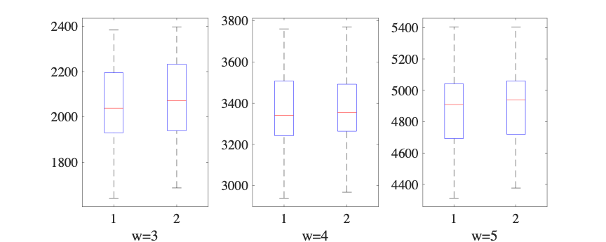
Figure 2: Comparison of profits generated by the two proposed solution approaches

In summary, if the computational scale of the optimization problem is small, i.e., $w$ is less than 5, the MISOCP reformulation approach is preferred. Otherwise, the two-step approach performs significantly better for large-scale optimization problems.

5.3 Comparison with Other Benchmarks

In this section, we validate the effectiveness of the proposed joint optimization model by comparing it with other commonly used benchmarks. Therefore, we first describe the three benchmarks used in practice, with details as follows:

Benchmark 1 (BM-1): Consistent EW design. This approach focuses mainly on the general EW design while ignoring the differences in automobile groups based on their initial prices, which are prevalent in current markets.

Benchmark 2 (BM-2): Personalized EW design. Different from Benchmark 1, this approach fully considers the diversities in different automobile groups. The formulation of this benchmark closely resembles that in Step 1 of the two-step approach. This benchmark is used to emphasize the importance of pricing and the necessity of joint optimization.

Benchmark 3 (BM-3): Bundle pricing with consistent design. This approach also jointly optimizes the EW design and pricing, while different automobile groups are not considered. Compared to our proposed model, using a consistent EW design reduces the complexity of the joint optimization model.

Notably, we provide more details about the model design and the corresponding solutions for these three benchmarks in Appendix C.

5.3.1 Performance Comparison

The performances of different models are evaluated by the mean profit under 30 replications. Specifically, we present different price initialization of each subsystem $P_{kj}$, which is realized by the change of its ratio to warranty cost $c_{kj}$, i.e., $c_{kj}=\gamma P_{kj}$. We use the percentages of profit improvement (denoted by Benefit(%)) to evaluate the performance of different approaches. Table 5 shows the average profits based on our proposed model, three benchmarks, and the corresponding percentage improvements. Notably, the joint optimization model yields the highest profit values between the two proposed solutions (i.e., MISOCP reformulation and two-step approaches) within a computation time of 600 seconds. We also present the corresponding solutions based on the proposed two approaches and three benchmarks in Figure 3. The horizontal axes represent the index of EW contracts, and the vertical axes present the customer groups, advertising list, and price discount ladders for $x_{ij}$, $y_{i}$, and $z_{ih}$, respectively. The EW contract offer to customers and the corresponding discount selected are colored blue. Contracts that are not recommended to customers do not require pricing and are colored gray.

Table 5: Performance comparison with three benchmarks

$w$	$\gamma$	Profit					Benefit(%)
		Joint	BM-1	BM-2	BM-3		BM-1	BM-2	BM-3
3	3	2954.08	2587.06	2642.02	2845.63		14.20	11.83	3.81
	6	2076.29	1742.90	1771.28	2009.86		19.29	17.42	3.33
	9	1213.76	905.37	922.89	1184.25		37.58	34.78	2.54
4	3	4776.09	4000.76	4072.99	4632.51		19.39	17.27	3.10
	6	3381.75	2621.66	2664.64	3284.39		29.09	27.03	2.97
	9	1989.77	1271.10	1320.57	1948.32		57.94	51.62	1.93
5	3	6934.77	5598.22	5598.22	6646.35		26.02	23.89	4.37
	6	4926.63	3516.56	3574.34	4749.31		40.25	38.02	3.80
	9	2964.20	1663.03	1737.39	2890.16		80.33	72.41	2.46
*Benefit(%)=[Profit(Joint)$-$Profit(BM)]/Profit(BM)$\times$ 100

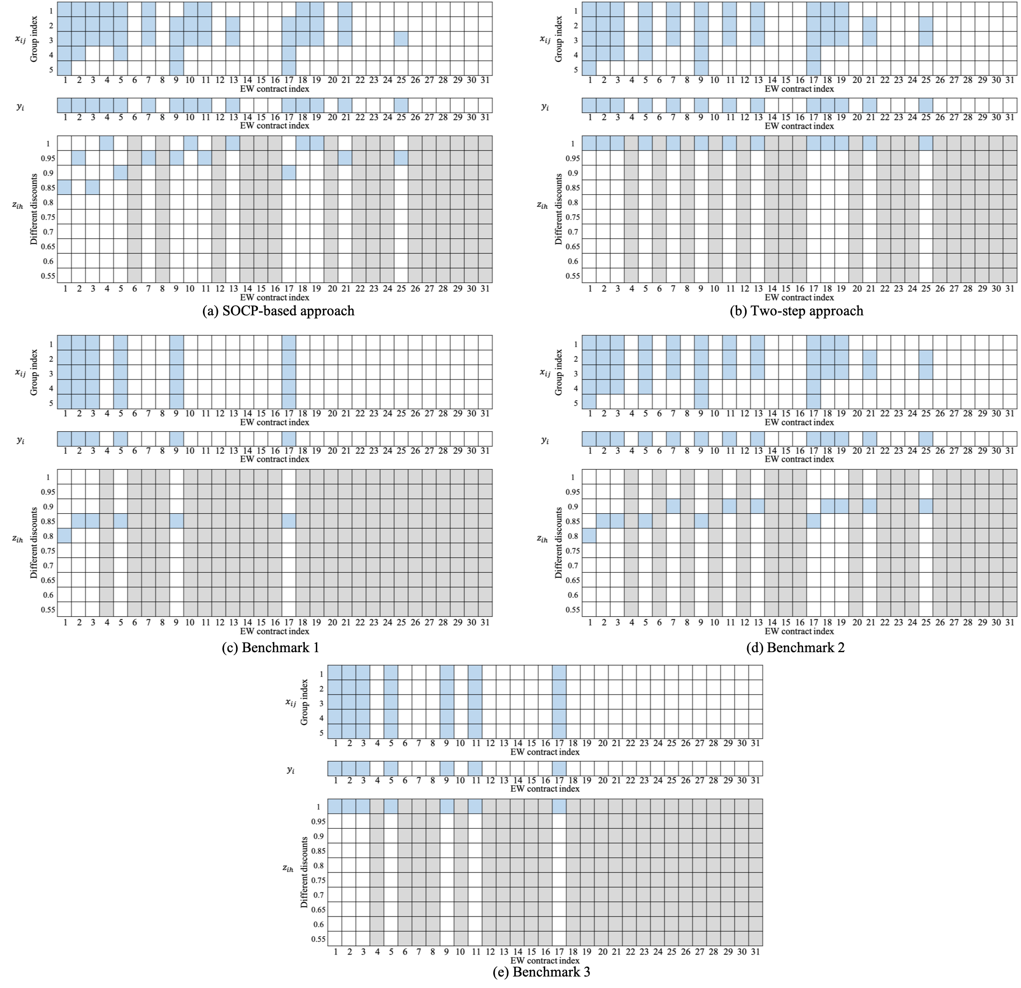
Figure 3: Illustration of solutions based on different approaches

By comparing the profit of the joint model with that in BM-1, BM-2, and BM-3 in Table 5, we can demonstrate the importance of joint optimization of EW design and pricing. In particular, with the increased number of subsystems $w$, the benefits of joint optimization become more significant. Due to the exponential increase in potential optimization choices with the growth in $w$, setting reasonable prices becomes particularly crucial in the optimization of problems involving more systems.

Besides the impact of subsystems, the initial prices also affect the total profit and the percentage of benefits. Figure 4 illustrates the effect of parameter $\gamma$ on the percentage of benefits of our proposed approach compared with three benchmarks. Specifically, the mean and standard errors of the benefit percentage are presented. Given the warranty cost for each subsystem, a larger $\gamma$ corresponds to a lower initial price, which leads significant profit decrease. Therefore, it is advisable for EW providers to slightly increase initial prices for opportunities to offer discounts in bundling pricing.

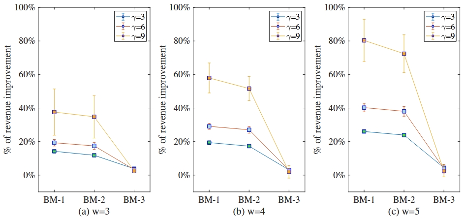
Figure 4: Performances comparison with different benchmarks

In summary, through the performance comparison with three benchmarks, we demonstrate the significant impact of joint design and pricing on total profit and provide the corresponding strategies from the perspective of EW providers. Furthermore, this section also validates the effectiveness of the proposed solution approaches, showing that they can ensure relatively high profits within the given computation time, regardless of the number of subsystems.

5.3.2 Robustness Check of Different Solution Approaches

In this subsection, we test the robustness of our proposed methods based on different distributions of customers’ utility ($v_{kj}$) on subsystems, as it directly influences customers’ purchase probabilities as well as EW providers’ profits. Besides Uniform distribution, we also discuss the profits and their gaps based on different optimization models when the value of $v_{kj}$ follows other distributions such as Power law and Normal distributions.

Table 6 presents the results based on different utility distributions. As shown, the joint optimization model proposed in our work consistently demonstrates significant advantages. Regardless of the distribution type, the profit improvement percentage compared to the other three benchmarks remains stable. This result effectively demonstrates the robustness of the proposed joint optimization approaches.

Table 6: Effect of Utility Distribution on Total Profits

$w$	Uti. Distri.	Profit					Benefit(%)
		Joint	BM-1	BM-2	BM-3		BM-1	BM-2	BM-3
3	Uniform	2104.54	1768.63	1800.40	2038.90		19.14	17.05	3.26
	Normal	2106.08	1768.97	1800.82	2039.56		19.21	17.11	3.30
	Power Law	2355.43	1936.35	1982.21	2269.35		21.79	18.97	3.84
4	Uniform	3407.91	2650.01	2688.97	3308.23		28.71	26.84	3.02
	Normal	3408.88	2650.62	2689.91	3309.28		28.71	26.84	3.01
	Power Law	3742.63	2840.72	2886.65	3603.46		31.87	29.76	3.89
5	Uniform	4972.06	3562.40	3611.09	4790.18		39.85	38.00	3.81
	Normal	4972.55	3560.68	3610.79	4786.13		39.95	38.04	3.99
	Power Law	5409.43	3781.09	3830.93	5206.34		43.43	41.57	4.05
*Benefit(%)=[Profit(Joint)$-$Profit(BM)]/Profit(BM)$\times$ 100

5.4 Effect of Other Factors on Total Profit

We now explore additional factors related to customers and the failure rate to derive relevant managerial insights. Section 5.4.1 addresses the composition of different groups of customers, while Section 5.4.2 examines the impact of the subsystems’ failure rates.

5.4.1 Composition of Customers

Customers who purchase automobiles from different price bands in the market have varying potential values. In this subsection, we consider five groups of customers with different values: the first group has the lowest value, while the fifth group has the highest. As shown in Figure 5, we examine three cases based on different customer compositions. In case 1, each group of customers is equally represented. In case 2, the proportion of customers decreases as their value increases, with the highest proportion being the lowest-value customers. In case 3, the customer distribution is symmetrical, with the highest proportion belonging to medium-value customers, and lower proportions for both high and low-value customers.

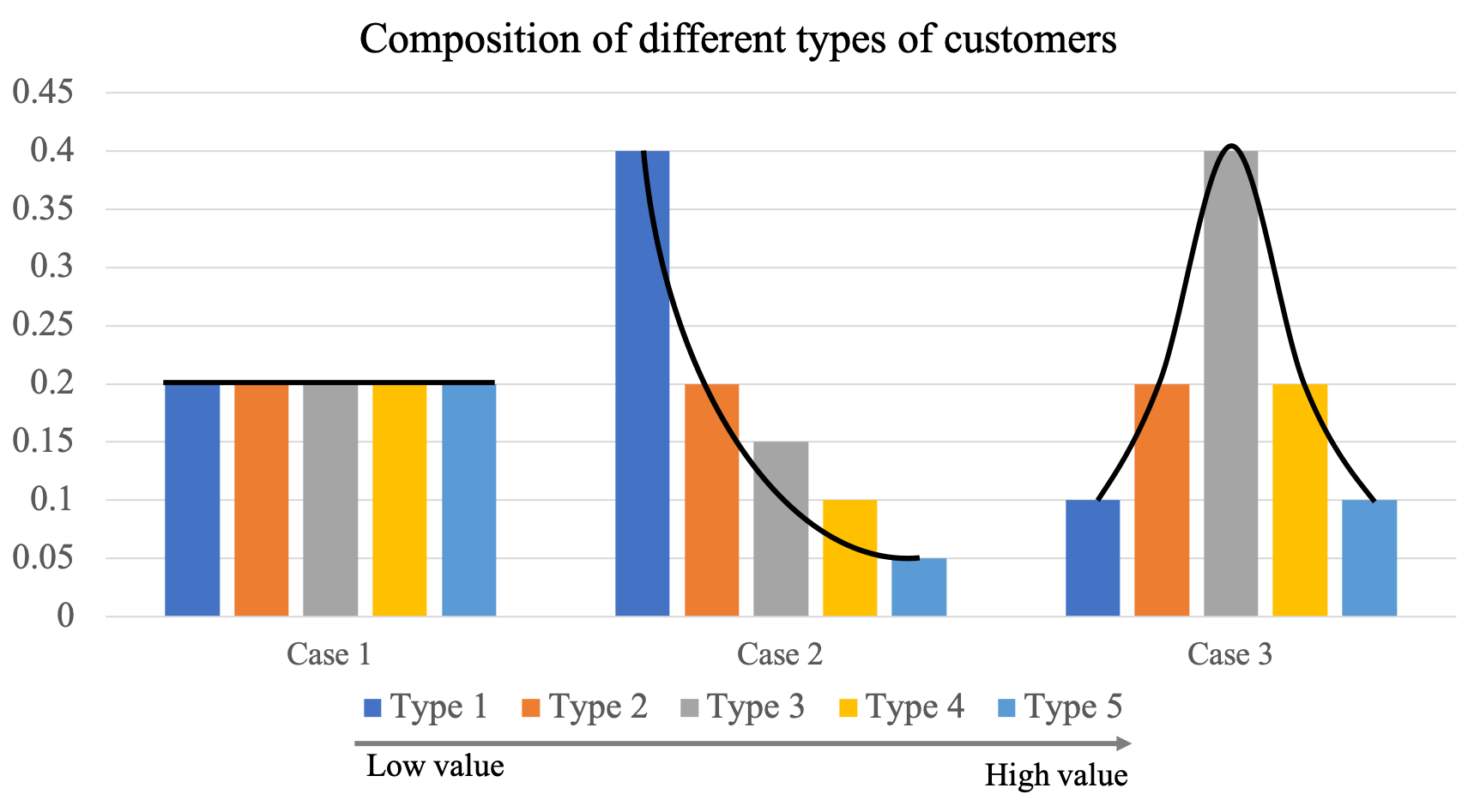
Figure 5: Composition of different groups of customers

Table 7: Effect of Customer Composition on Total Profits

$w$	Cases	Profit					Benefit(%)
		Joint	BM-1	BM-2	BM-3		BM-1	BM-2	BM-3
3	case 1	2076.29	1742.90	1771.28	2009.86		19.29	17.42	3.33
	case 2	730.83	621.96	634.01	705.64		17.56	15.33	3.57
	case 3	1470.21	1253.31	1277.25	1417.63		17.36	15.18	3.70
4	case 1	3381.75	2621.66	2664.64	3284.39		29.09	27.03	2.97
	case 2	1240.38	997.62	1010.04	1211.55		24.39	22.87	2.37
	case 3	2472.64	1966.35	1997.76	2404.73		25.86	23.90	2.82
5	case 1	4926.63	3516.56	3574.34	4749.31		40.25	38.02	3.80
	case 2	1820.51	1372.31	1393.99	1708.69		32.74	30.69	6.65
	case 3	3584.12	2625.48	2672.33	3414.00		36.68	34.31	5.04
*Benefit(%)=[Profit(Joint)$-$Profit(BM)]/Profit(BM) $\times$ 100

Table 7 illustrates the EW profits based on the cases with different compositions of customer groups. We find that the uniform proportion of different groups of customers in case 1 leads to higher profit regardless of $w$. This phenomenon implies the importance of high-value customers, which are the main source of profits for manufacturers. Even replacing low-value and high-value customers with medium-value customers does not result in profit increases compared to a uniform proportion. Therefore, attracting and retaining high-value customers is a crucial consideration for providers in EW promotion. Additionally, we find that when the benchmark methods (particularly BM-1 and BM-2) are applied in case 1, where there is a high proportion of high-value customers, the profit gap becomes larger. This phenomenon further demonstrates the necessity of joint optimization, which provides reasonable prices for customers. Since high-value customers contribute more profit for EW providers, the effectiveness of the joint model becomes increasingly significant as the proportion of high-value customers rises.

5.4.2 Effect of Failure Rate

The failure rate is one of the most important factors that impact the profit of EW providers. Therefore, in this section, we focus mainly on different failure rates of function systems. Table 8 illustrates the profit and the corresponding gaps based on different solution approaches when failure rates follow a uniform distribution with varying parameters. It is obvious that the failure rate significantly decreases the EW providers’ profit.

Table 8: Effect of Failure Rate on Total Profits

$w$	Failure rate	Profit					Benefit(%)
		Joint	BM-1	BM-2	BM-3		BM-1	BM-2	BM-3
3	U(0.01,0.05)	3166.79	2793.49	2857.44	3053.02		13.40	10.86	3.74
	U(0.05,0.10)	2078.83	1742.91	1775.35	2013.81		19.37	17.20	3.24
	U(0.10,0.15)	966.77	663.83	674.70	950.55		48.80	46.09	1.71
4	U(0.01,0.05)	5059.85	4277.58	4361.40	4897.96		18.30	16.03	3.31
	U(0.05,0.10)	3397.43	2636.53	2676.67	3294.78		29.00	27.08	3.13
	U(0.10,0.15)	1429.83	753.79	780.28	1401.62		93.36	86.59	2.02
5	U(0.01,0.05)	7278.56	5865.17	5975.62	6942.29		24.12	21.83	4.88
	U(0.05,0.10)	4919.05	3512.21	3565.57	4731.95		40.12	38.05	4.00
	U(0.10,0.15)	2158.36	969.34	1009.18	2089.11		125.23	115.70	3.41
*Benefit(%)=[Profit(Joint)$-$Profit(BM)]/Profit(BM)$\times$ 100

Interestingly, by comparing the proposed joint optimization with BM-1 and BM-2 methods, we find that the advantages of jointly optimizing design and pricing become significant, especially when the failure rate is high or the number of systems is large. In comparison with BM-3, which is a simplified version of our joint optimization model, recommending the same EW design for different automobile groups, its computational complexity is lower than that of the joint optimization model presented in Section 3. Table 8 reveals that the profit gap between BM-3 and our proposed method decreases with the failure rate but increases with the number of subsystems. This finding suggests that in scenarios with a limited number of systems or a higher occurrence of failures, BM-3 can be regarded as a viable substitute for the joint optimization model.

6 Conclusions

This work addresses a prevalent optimization problem faced by third-party automotive EW providers in the aftermarket, aiming to maximize total profits. We develop a joint optimization model for EW design and pricing based on automobiles with different price bands. Given the computational complexity of the model, we propose two solution approaches, namely, the MISOCP formulation and two-step iterated approaches. We develop corresponding algorithms for each approach to provide detailed procedural descriptions, and the corresponding theoretical properties are also guaranteed. Our numerical experiments demonstrate the advantages of our solution approaches, particularly when the failure rate is high and the number of subsystems is large. We also verify the importance of high-value customers, which is the main source of profits for EW providers.

Our paper is the pioneer work to jointly optimize the EW design and pricing from the perspective of different subsystems. Along with our work, there are several potential directions for future research. First, with the proliferation of intelligent and connected automobiles, considering customers’ personalized driving behaviors in the design and pricing of EW contracts is an important research direction. Second, the design of EW services should consider fairness among different groups of customers to meet the needs of a larger number of customers in the market.

Data Availability Statement

The authors confirm that the data supporting the findings of this study are available within the article.

Supplemental Online Materials to “Joint Design and Pricing of Extended Warranties for Multiple Automobiles with Different Price Bands”

Appendix A Notations

Table 9: Notations

Sets
$\mathcal{M}=\{1,2,\dots,m\}$	: Set of groups of automobiles
$\mathcal{W}=\{1,2,\dots,w\}$	: Set of systems in each automobile
$\mathcal{N}=\{1,2,\dots,n\}$	: Set of EW contracts, with $n=2^{w}-1$
$\mathcal{L}=\{1,2,\dots,l\}$	: Set of discount ladders
Indices
$i\in\mathcal{N}$	: Index of EW contract
$j\in\mathcal{M}$	: Index of automobile groups
$k\in\mathcal{W}$	: Index of subsystems
$h\in\mathcal{L}$	: Index of discounts
Parameters
$d_{h}$	: Discount level of the $h$th ladder
$v_{kj}$	: Net utility of system $k$ for customers in group $j$
$u_{0j}$	: Net utility of the no-purchase option for customers in group $j$
$P_{kj}^{0}$	: Initial selling price of system $k$ in automobiles belonging to group $j$
$\beta_{j}$	: Price sensitivity of customers in group $j$
$\mathbb{I}_{ik}$	: Binary value indicating whether contract $i$ includes system $k$
$\lambda_{j}$	: The proportion of group-$j$ customers
$f_{kj}$	: Failure probability of system $k$ in automobiles belonging to group $j$
$c_{kj}$	: Failure cost of system $k$ in automobiles belonging to group $j$
$\theta$	: Advertising cost of an EW
Decision variables
$p_{ij}$	: Selling price of EW contract $i$ for customers in group $j$
$x_{ij}$	: Binary variable indicating whether EW contract $i$ is recommended to automobiles in group $j$
$y_{i}$	: Binary variable indicating whether EW contract $i$ is in advertising list
$z_{ih}$	: Binary variable indicating whether the discount of contract $i$ is $d_{h}$

Appendix B Reformulations of Problem (JDPEW) Based on the Two-step Iterated Approach

 

B.1 Reformulation of Step 1

Let

$$t_{j}=\frac{1}{u_{0j}+\sum_{i\in\mathcal{N}}\left[\hat{V}_{ij}-\beta_{j}\hat{P}_{ij}\left(\sum_{h\in\mathcal{L}}z_{ih}^{*}d_{h}\right)\right]x_{ij}}$$

and

$$w_{j}=u_{0j}+\sum_{i\in\mathcal{N}}\left[\hat{V}_{ij}-\beta_{j}\hat{P}_{ij}\left(\sum_{h\in\mathcal{L}}z_{ih}^{*}d_{h}\right)\right]x_{ij}.$$

Then, model (JDPEW) can be reformulated as (JDPEW’):

$$\min\quad \sum_{j\in\mathcal{M}}\lambda_{j}u_{0j}\hat{R}_{j}t_{j}+\sum_{i\in\mathcal{N}}\theta y_{i}+\sum_{j\in\mathcal{M}}\lambda_{j}\sum_{i\in\mathcal{N}}\left(\hat{V}_{ij}\hat{R}_{j}x_{ij}-\hat{V}_{ij}\hat{P}_{ij}\left(\sum_{h\in\mathcal{L}}z_{ih}^{*}x_{ij}d_{h}\right)+\hat{V}_{ij}\hat{C}_{ij}x_{ij}\right)t_{j}+$$

$$\sum_{j\in\mathcal{M}}\lambda_{j}\sum_{i\in\mathcal{N}}\left(-\beta_{j}\hat{R}_{j}\hat{P}_{ij}\left(\sum_{h\in\mathcal{L}}z_{ih}^{*}x_{ij}d_{h}\right)+\beta_{j}\hat{P}_{ij}^{2}\left(\sum_{h\in\mathcal{L}}z_{ih}^{*}x_{ij}d_{h}^{2}\right)-\beta_{j}\hat{P}_{ij}\left(\sum_{h\in\mathcal{L}}z_{ih}^{*}x_{ij}d_{h}\right)\hat{C}_{ij}\right)t_{j}$$

s.t $$x_{ij}\leq y_{i}\hskip 180.00027pt\forall i\in\mathcal{N},\leavevmode\nobreak\ j\in\mathcal{M}\hskip 80.00012pt$$

$$\sum_{i\in\mathcal{N}}\mathbb{I}_{ik}x_{ij}\geq 1\hskip 155.00023pt\forall k\in\mathcal{W},\leavevmode\nobreak\ j\in\mathcal{M}\hskip 80.00012pt$$

$$y_{i}\in\{0,1\},x_{ij}\in\{0,1\}\hskip 120.00018pt\forall i\in\mathcal{N},\leavevmode\nobreak\ j\in\mathcal{M}.\hskip 80.00012pt$$

Let $g_{ij}=t_{j}x_{ij}$. Similarly, we can replace this equality with constraints (33)-(36):

$$g_{ij}\geq t_{j}+\left(x_{ij}-1\right)t_{j}^{U}\quad \forall i\in\mathcal{N},\leavevmode\nobreak\ j\in\mathcal{M}$$ (33)

$$g_{ij}\geq x_{ij}t_{j}^{L}\quad \forall i\in\mathcal{N},\leavevmode\nobreak\ j\in\mathcal{M}$$ (34)

$$g_{ij}\leq t_{j}+\left(x_{ij}-1\right)t_{j}^{L}\quad \forall i\in\mathcal{N},\leavevmode\nobreak\ j\in\mathcal{M}$$ (35)

$$g_{ij}\leq x_{ij}t_{j}^{U}\quad \forall i\in\mathcal{N},\leavevmode\nobreak\ j\in\mathcal{M},$$ (36)

where $t_{j}^{L}=1/(u_{0j}+\sum_{i\in\mathcal{N}}\hat{V}_{ij})$ and $t_{j}^{U}=1/u_{0j}$.

Step 1 can finally be transformed into the following model that can be solved directly with existing solvers:

$$\min\quad \sum_{j\in\mathcal{M}}\lambda_{j}u_{0j}\hat{R}_{j}t_{j}+\sum_{i\in\mathcal{N}}\theta y_{i}+\sum_{j\in\mathcal{M}}\lambda_{j}\sum_{i\in\mathcal{N}}\left(\hat{V}_{ij}\hat{R}_{j}g_{ij}-\hat{V}_{ij}\hat{P}_{ij}\left(\sum_{h\in\mathcal{L}}z_{ih}^{*}g_{ij}d_{h}\right)+\hat{V}_{ij}\hat{C}_{ij}g_{ij}\right)+\qquad$$

$$\sum_{j\in\mathcal{M}}\lambda_{j}\sum_{i\in\mathcal{N}}\left(-\beta_{j}\hat{R}_{j}\hat{P}_{ij}\left(\sum_{h\in\mathcal{L}}z_{ih}^{*}g_{ij}d_{h}\right)+\beta_{j}\hat{P}_{ij}^{2}\left(\sum_{h\in\mathcal{L}}z_{ih}^{*}g_{ij}d_{h}^{2}\right)-\beta_{j}\hat{P}_{ij}\left(\sum_{h\in\mathcal{L}}z_{ih}^{*}g_{ij}d_{h}\right)\hat{C}_{ij}\right)$$

s.t $$x_{ij}\leq y_{i} \forall i\in\mathcal{N},\leavevmode\nobreak\ j\in\mathcal{M}\qquad\qquad\qquad\qquad$$

$$\sum_{i\in\mathcal{N}}\mathbb{I}_{ik}x_{ij}\geq 1 \forall k\in\mathcal{W},\leavevmode\nobreak\ j\in\mathcal{M}$$

$$t_{j}w_{j}\geq 1\quad \forall j\in\mathcal{M}$$

$$w_{j}=u_{0j}+\sum_{i\in\mathcal{N}}\left[\hat{V}_{ij}x_{ij}-\beta_{j}\hat{P}_{ij}\left(\sum_{h\in\mathcal{L}}z_{ih}^{*}x_{ij}d_{h}\right)\right] \forall j\in\mathcal{M}$$

$$g_{ij}\geq t_{j}+\left(x_{ij}-1\right)t_{j}^{U}\quad \forall i\in\mathcal{N},\leavevmode\nobreak\ j\in\mathcal{M}$$

$$g_{ij}\geq x_{ij}t_{j}^{L}\quad \forall i\in\mathcal{N},\leavevmode\nobreak\ j\in\mathcal{M}$$

$$g_{ij}\leq t_{j}+\left(x_{ij}-1\right)t_{j}^{L}\quad \forall i\in\mathcal{N},\leavevmode\nobreak\ j\in\mathcal{M}$$

$$g_{ij}\leq x_{ij}t_{j}^{U}\quad \forall i\in\mathcal{N},\leavevmode\nobreak\ j\in\mathcal{M}$$

$$y_{i}\in\{0,1\},x_{ij}\in\{0,1\},t_{j}\geq 0,w_{j}\geq 0 \forall i\in\mathcal{N},\leavevmode\nobreak\ j\in\mathcal{M}.$$

 

B.2 Reformulation of Step 2

Let

$$t_{j}=\frac{1}{u_{0j}+\sum_{i\in\mathcal{N}}\left[\hat{V}_{ij}-\beta_{j}\hat{P}_{ij}\left(\sum_{h\in\mathcal{L}}z_{ih}d_{h}\right)\right]x_{ij}^{*}}$$

and

$$w_{j}=u_{0j}+\sum_{i\in\mathcal{N}}\left[\hat{V}_{ij}-\beta_{j}\hat{P}_{ij}\left(\sum_{h\in\mathcal{L}}z_{ih}d_{h}\right)\right]x_{ij}^{*}.$$

Then, model (JDPEW) can be reformulated as (JDPEW’’):

$$\min\quad \sum_{j\in\mathcal{M}}\lambda_{j}u_{0j}\hat{R}_{j}t_{j}+\sum_{i\in\mathcal{N}}\theta y_{i}^{*}+\sum_{j\in\mathcal{M}}\lambda_{j}\sum_{i\in\mathcal{N}}\left(\hat{V}_{ij}\hat{R}_{j}x_{ij}^{*}-\hat{V}_{ij}\hat{P}_{ij}\left(\sum_{h\in\mathcal{L}}z_{ih}x_{ij}^{*}d_{h}\right)+\hat{V}_{ij}\hat{C}_{ij}x_{ij}^{*}\right)t_{j}+$$

$$\sum_{j\in\mathcal{M}}\lambda_{j}\sum_{i\in\mathcal{N}}\left(-\beta_{j}\hat{R}_{j}\hat{P}_{ij}\left(\sum_{h\in\mathcal{L}}z_{ih}x_{ij}^{*}d_{h}\right)+\beta_{j}\hat{P}_{ij}^{2}\left(\sum_{h\in\mathcal{L}}z_{ih}x_{ij}^{*}d_{h}^{2}\right)-\beta_{j}\hat{P}_{ij}\left(\sum_{h\in\mathcal{L}}z_{ih}x_{ij}^{*}d_{h}\right)\hat{C}_{ij}\right)t_{j}$$

s.t $$\sum_{h\in\mathcal{L}}z_{ih}=1\hskip 190.00029pt\forall i\in\mathcal{N}\hskip 40.00006pt$$

$$\left(\sum_{h\in\mathcal{L}}z_{ih}d_{h}-\sum_{h^{\prime}\in L}z_{i^{\prime}h^{\prime}}d_{h^{\prime}}\right)\left(\sum_{k\in\mathcal{W}}\mathbb{I}_{ik}-\sum_{k\in\mathcal{W}}\mathbb{I}_{i^{\prime}k}\right)\leq 0\hskip 10.00002pt\forall i,\leavevmode\nobreak\ i^{\prime}\in\mathcal{N}\hskip 40.00006pt$$

$$p_{ij}=\left(\sum_{k\in\mathcal{W}}\mathbb{I}_{ik}P_{kj}^{0}\right)\left(\sum_{h\in\mathcal{L}}z_{ih}d_{h}\right)\hskip 93.00017pt\forall i\in\mathcal{N},\leavevmode\nobreak\ j\in\mathcal{M}$$ (37)

$$z_{ih}\in\{0,1\}\hskip 195.00029pt\forall i\in\mathcal{N},\leavevmode\nobreak\ h\in\mathcal{L}.\hskip 70.0001pt$$

Let $g_{ijh}=t_{j}z_{ih}$. Similarly, we can replace this equality with constraints (38)-(41):

$$g_{ijh}\geq t_{j}+\left(z_{ih}-1\right)t_{j}^{U}\quad \forall i\in\mathcal{N},\leavevmode\nobreak\ j\in\mathcal{M}$$ (38)

$$g_{ijh}\geq z_{ih}t_{j}^{L}\quad \forall i\in\mathcal{N},\leavevmode\nobreak\ j\in\mathcal{M}$$ (39)

$$g_{ijh}\leq t_{j}+\left(z_{ih}-1\right)t_{j}^{L}\quad \forall i\in\mathcal{N},\leavevmode\nobreak\ j\in\mathcal{M}$$ (40)

$$g_{ijh}\leq z_{ih}t_{j}^{U}\quad \forall i\in\mathcal{N},\leavevmode\nobreak\ j\in\mathcal{M},$$ (41)

where $t_{j}^{L}=1/(u_{0j}+\sum_{i\in\mathcal{N}}\hat{V}_{ij})$ and $t_{j}^{U}=1/u_{0j}$.

Finally, Step 2 can be transformed into the following model that can be solved directly with existing solvers:

$$\min\quad \sum_{j\in\mathcal{M}}\lambda_{j}u_{0j}\hat{R}_{j}t_{j}+\sum_{i\in\mathcal{N}}\theta y_{i}^{*}+\sum_{j\in\mathcal{M}}\lambda_{j}\sum_{i\in\mathcal{N}}\left(\hat{V}_{ij}\hat{R}_{j}x_{ij}^{*}t_{j}-\hat{V}_{ij}\hat{P}_{ij}\left(\sum_{h\in\mathcal{L}}g_{ijh}x_{ij}^{*}d_{h}\right)+\hat{V}_{ij}\hat{C}_{ij}x_{ij}^{*}t_{j}\right)+\qquad$$

$$\sum_{j\in\mathcal{M}}\lambda_{j}\sum_{i\in\mathcal{N}}\left(-\beta_{j}\hat{R}_{j}\hat{P}_{ij}\left(\sum_{h\in\mathcal{L}}g_{ijh}x_{ij}^{*}d_{h}\right)+\beta_{j}\hat{P}_{ij}^{2}\left(\sum_{h\in\mathcal{L}}g_{ijh}x_{ij}^{*}d_{h}^{2}\right)-\beta_{j}\hat{P}_{ij}\left(\sum_{h\in\mathcal{L}}g_{ijh}x_{ij}^{*}d_{h}\right)\hat{C}_{ij}\right)$$

s.t $$\sum_{h\in\mathcal{L}}z_{ih}=1 \forall i\in\mathcal{N}$$

$$\left(\sum_{h\in\mathcal{L}}z_{ih}d_{h}-\sum_{h^{\prime}\in L}z_{i^{\prime}h^{\prime}}d_{h^{\prime}}\right)\left(\sum_{k\in\mathcal{W}}\mathbb{I}_{ik}-\sum_{k\in\mathcal{W}}\mathbb{I}_{i^{\prime}k}\right)\leq 0 \forall i\in\mathcal{N},i^{\prime}\in N$$

$$p_{ij}=\left(\sum_{k\in\mathcal{W}}\mathbb{I}_{ik}P_{kj}^{0}\right)\left(\sum_{h\in\mathcal{L}}z_{ih}d_{h}\right) \forall i\in\mathcal{N},\leavevmode\nobreak\ j\in\mathcal{M}$$

$$t_{j}w_{j}\geq 1\quad \forall j\in\mathcal{M}$$

$$w_{j}=u_{0j}+\sum_{i\in\mathcal{N}}\left[\hat{V}_{ij}x_{ij}^{*}-\beta_{j}\hat{P}_{ij}\left(\sum_{h\in\mathcal{L}}z_{ih}x_{ij}^{*}d_{h}\right)\right] \forall j\in\mathcal{M}$$

$$g_{ijh}\geq t_{j}+\left(z_{ih}-1\right)t_{j}^{U}\quad \forall i\in\mathcal{N},j\in\mathcal{M},h\in\mathcal{L}$$

$$g_{ijh}\geq z_{ih}t_{j}^{L}\quad \forall i\in\mathcal{N},j\in\mathcal{M},h\in\mathcal{L}$$

$$g_{ijh}\leq t_{j}+\left(z_{ih}-1\right)t_{j}^{L}\quad \forall i\in\mathcal{N},j\in\mathcal{M},h\in\mathcal{L}$$

$$g_{ijh}\leq z_{ih}t_{j}^{U}\quad \forall i\in\mathcal{N},j\in\mathcal{M},h\in\mathcal{L}$$

$$z_{ih}\in\{0,1\} \forall i\in\mathcal{N},h\in\mathcal{L}.$$

 

Appendix C Benchmark Models

 

C.1 Benchmark 1: Consistent EW Design

Let $z_{ih}^{0}$ denote the initial value of $z_{ih}$, where $z_{ih}^{0}$ is calculated as follows:

$$\begin{aligned} &z_{ih}^{0}=\begin{cases}1&\text{ if }h=\operatorname{argmax}_{k\in W}\{k:\mathbb{I}_{ik}=1\}\\ 0&\text{ otherwise }\end{cases}\\ \end{aligned}.$$

The model of the consistent warranty design for all segments is as follows:

$$\max\quad \sum_{j\in\mathcal{M}}\lambda_{j}q_{ij}\left(z_{ih}^{0},x_{i}\right)\cdot\sum_{i\in\mathcal{N}}\left[\left(\sum_{k\in\mathcal{W}}\mathbb{I}_{ik}P_{kj}\right)\left(\sum_{h\in\mathcal{L}}z_{ih}^{0}d_{h}\right)-\sum_{k\in\mathcal{W}}\mathbb{I}_{ik}f_{kj}c_{jk}\right]-\sum_{i\in\mathcal{N}}\theta x_{i}$$

s.t $$\sum_{i\in\mathcal{N}}\mathbb{I}_{ik}x_{i}\geq 1 \forall k\in\mathcal{W}\quad\quad$$

$$x_{i}\in\{0,1\} \forall i\in\mathcal{N},$$

where $q_{ij}\left(z^{0}_{ih},x_{ij}\right)$ is group-$j$ customers’ choice probability of EW contract $i$. The structure of the function remains similar to what is described in Equation (3), with $z_{ih}$ replaced by $z^{0}_{ih}$.

Through a series of transformations of the above model, the final model to be solved after reformulation is as follows:

$$\min\quad \sum_{j\in\mathcal{M}}\lambda_{j}u_{0j}\hat{R}_{j}t_{j}+\sum_{i\in\mathcal{N}}\theta x_{i}+\sum_{j\in\mathcal{M}}\lambda_{j}\sum_{i\in\mathcal{N}}\bigg{[}\hat{V}_{ij}\hat{R}_{j}g_{ij}-\hat{V}_{ij}\hat{P}_{ij}\left(\sum_{h\in\mathcal{L}}z_{ih}^{0}g_{ij}d_{h}\right)+\hat{V}_{ij}\hat{C}_{ij}g_{ij}$$

$$-\beta_{j}\hat{R}_{j}\hat{P}_{ij}\left(\sum_{h\in\mathcal{L}}z_{ih}^{0}g_{ij}d_{h}\right)+\beta_{j}\hat{P}_{ij}^{2}\left(\sum_{h\in\mathcal{L}}z_{ih}^{0}g_{ij}d_{h}^{2}\right)-\beta_{j}\hat{P}_{ij}\left(\sum_{h\in\mathcal{L}}z_{ih}^{0}g_{ij}d_{h}\right)\hat{C}_{ij}\bigg{]}$$

s.t $$\sum_{i\in\mathcal{N}}\mathbb{I}_{ik}x_{i}\geq 1 \forall k\in\mathcal{W}$$

$$t_{j}w_{j}\geq 1 \forall j\in\mathcal{M}$$

$$w_{j}=u_{0j}+\sum_{i\in\mathcal{N}}\left[\hat{V}_{ij}x_{i}-\beta_{j}\hat{P}_{ij}\left(\sum_{h\in\mathcal{L}}z_{ih}^{0}x_{i}d_{h}\right)\right] \forall j\in\mathcal{M}$$

$$g_{ij}\geq t_{j}+\left(x_{i}-1\right)t_{j}^{U} \forall i\in\mathcal{N},j\in\mathcal{M}$$

$$g_{ij}\geq x_{i}t_{j}^{L} \forall i\in\mathcal{N},j\in\mathcal{M}$$

$$g_{ij}\leq t_{j}+\left(x_{i}-1\right)t_{j}^{L} \forall i\in\mathcal{N},j\in\mathcal{M}$$

$$g_{ij}\leq x_{i}t_{j}^{U} \forall i\in\mathcal{N},j\in\mathcal{M}$$

$$x_{i}\in\{0,1\},t_{j}\geq 0,w_{j}\geq 0 \forall i\in\mathcal{N},j\in\mathcal{M}.$$

C.2 Benchmark 2: Personalized EW Design

This model is the same as Step 1 in Section 4.2.

$$\max\quad \sum_{j\in\mathcal{M}}\lambda_{j}\sum_{i\in\mathcal{N}}q_{ij}\left(z_{ih}^{0},x_{ij}\right)\left[\left(\sum_{k\in\mathcal{W}}\mathbb{I}_{ik}P_{kj}\right)\left(\sum_{h\in\mathcal{L}}z_{ih}^{0}d_{h}\right)-\sum_{k\in\mathcal{W}}\mathbb{I}_{ik}f_{kj}c_{jk}\right]-\sum_{i\in\mathcal{N}}\theta y_{i}$$

s.t $$x_{ij}\leq y_{i}\hskip 180.00027pt\forall i\in\mathcal{N},j\in\mathcal{M}$$

$$\sum_{i\in\mathcal{N}}\mathbb{I}_{ik}x_{ij}\geq 1\hskip 155.00023pt\forall k\in\mathcal{W},j\in\mathcal{M}$$

$$y_{i}\in\{0,1\},x_{ij}\in\{0,1\}\hskip 120.00018pt\forall i\in\mathcal{N},j\in\mathcal{M}.$$

Through a series of transformation of the above model, the final model to be solved after reformulation is as follows:

$$\min\quad \sum_{j\in\mathcal{M}}\lambda_{j}u_{0j}\hat{R}_{j}t_{j}+\sum_{i\in\mathcal{N}}\theta y_{i}+\sum_{j\in\mathcal{M}}\lambda_{j}\sum_{i\in\mathcal{N}}\left(\hat{V}_{ij}\hat{R}_{j}g_{ij}-\hat{V}_{ij}\hat{P}_{ij}\left(\sum_{h\in\mathcal{L}}z_{ih}^{*}g_{ij}d_{h}\right)+\hat{V}_{ij}\hat{C}_{ij}g_{ij}\right)+\qquad$$

$$\sum_{j\in\mathcal{M}}\lambda_{j}\sum_{i\in\mathcal{N}}\left(-\beta_{j}\hat{R}_{j}\hat{P}_{ij}\left(\sum_{h\in\mathcal{L}}z_{ih}^{*}g_{ij}d_{h}\right)+\beta_{j}\hat{P}_{ij}^{2}\left(\sum_{h\in\mathcal{L}}z_{ih}^{*}g_{ij}d_{h}^{2}\right)-\beta_{j}\hat{P}_{ij}\left(\sum_{h\in\mathcal{L}}z_{ih}^{*}g_{ij}d_{h}\right)\hat{C}_{ij}\right)$$

s.t $$x_{ij}\leq y_{i} \forall i\in\mathcal{N},j\in\mathcal{M}\qquad\qquad\qquad\qquad$$

$$\sum_{i\in\mathcal{N}}\mathbb{I}_{ik}x_{ij}\geq 1 \forall k\in\mathcal{W},j\in\mathcal{M}$$

$$t_{j}w_{j}\geq 1\quad \forall j\in\mathcal{M}$$

$$w_{j}=u_{0j}+\sum_{i\in\mathcal{N}}\left[\hat{V}_{ij}x_{ij}-\beta_{j}\hat{P}_{ij}\left(\sum_{h\in\mathcal{L}}z_{ih}^{*}x_{ij}d_{h}\right)\right] \forall j\in\mathcal{M}$$

$$g_{ij}\geq t_{j}+\left(x_{ij}-1\right)t_{j}^{U}\quad \forall i\in\mathcal{N},j\in\mathcal{M}$$

$$g_{ij}\geq x_{ij}t_{j}^{L}\quad \forall i\in\mathcal{N},j\in\mathcal{M}$$

$$g_{ij}\leq t_{j}+\left(x_{ij}-1\right)t_{j}^{L}\quad \forall i\in\mathcal{N},j\in\mathcal{M}$$

$$g_{ij}\leq x_{ij}t_{j}^{U}\quad \forall i\in\mathcal{N},j\in\mathcal{M}$$

$$y_{i}\in\{0,1\},x_{ij}\in\{0,1\},t_{j}\geq 0,w_{j}\geq 0 \forall i\in\mathcal{N},j\in\mathcal{M}.$$

 

C.3 Benchmark 3: Bundle Pricing with Consistent Design

This is a commonly used method in reality to recommend the same contract for all different groups of automobiles. This means that $x_{ij}=x_{ij^{\prime}}$ for all $j\neq j^{\prime}$. For convenience, we will denote it as $x_{i}$. Here, the decision variables are the contracts recommended for automobiles $x_{i}$, as well as the discount prices for each contract $z_{ih}$. The model of the same warranty design for all segments is as follows:

$$\max\quad\sum_{j\in\mathcal{M}}\lambda_{j}q_{ij}\left(z_{ih},x_{i}\right)\cdot\sum_{i\in\mathcal{N}}\left[\left(\sum_{k\in\mathcal{W}}\mathbb{I}_{ik}P_{kj}\right)\left(\sum_{h\in\mathcal{L}}z_{ih}d_{h}\right)-\sum_{k\in\mathcal{W}}\mathbb{I}_{ik}f_{kj}c_{jk}\right]-\sum_{i\in\mathcal{N}}\theta x_{i}$$

s.t $$\sum_{i\in\mathcal{N}}\mathbb{I}_{ik}x_{i}\geq 1 \forall k\in\mathcal{W}$$

$$\sum_{h\in\mathcal{L}}z_{ih}=1 \forall i\in\mathcal{N}$$

$$\left(\sum_{h\in\mathcal{L}}z_{ih}d_{h}-\sum_{h^{\prime}\in L}z_{i^{\prime}h^{\prime}}d_{h^{\prime}}\right)\left(\sum_{k\in\mathcal{W}}\mathbb{I}_{ik}-\sum_{k\in\mathcal{W}}\mathbb{I}_{i^{\prime}k}\right)\leq 0 \forall i\in\mathcal{N},\leavevmode\nobreak\ i\in\mathcal{N}$$

$$p_{ij}=\left(\sum_{k\in\mathcal{W}}\mathbb{I}_{ik}P_{kj}^{0}\right)\left(\sum_{h\in\mathcal{L}}z_{ih}d_{h}\right) \forall i\in\mathcal{N},\leavevmode\nobreak\ j\in\mathcal{M}$$

$$x_{i}\in\{0,1\},z_{ih}\in\{0,1\} \forall i\in\mathcal{N},h\in\mathcal{L}.$$

Through a series of transformations of the above model, the final model to be solved after reformulation is as follows:

$$\min\quad \sum_{j\in\mathcal{M}}\lambda_{j}u_{0j}\hat{R}_{j}t_{j}+\sum_{i\in\mathcal{N}}\theta x_{i}+\sum_{j\in\mathcal{M}}\lambda_{j}\sum_{i\in\mathcal{N}}\bigg{[}\hat{V}_{ij}\hat{R}_{j}g_{ij}-\hat{V}_{ij}\hat{P}_{ij}\left(\sum_{h\in\mathcal{L}}o_{ijh}d_{h}\right)+\hat{V}_{ij}\hat{C}_{ij}g_{ij}\qquad\quad$$

$$-\beta_{j}\hat{R}_{j}\hat{P}_{ij}\left(\sum_{h\in\mathcal{L}}o_{ijh}d_{h}\right)+\beta_{j}\hat{P}_{ij}^{2}\left(\sum_{h\in\mathcal{L}}o_{ijh}d_{h}^{2}\right)-\beta_{j}\hat{P}_{ij}\left(\sum_{h\in\mathcal{L}}o_{ijh}d_{h}\right)\hat{C}_{ij}\bigg{]}$$

s.t $$\sum_{i\in\mathcal{N}}\mathbb{I}_{ik}x_{i}\geq 1 \forall k\in\mathcal{W}$$

$$\sum_{h\in\mathcal{L}}z_{ih}=1 \forall i\in\mathcal{N}$$

$$\left(\sum_{h\in\mathcal{L}}z_{ih}d_{h}-\sum_{h^{\prime}\in L}z_{i^{\prime}h^{\prime}}d_{h^{\prime}}\right)\left(\sum_{k\in\mathcal{W}}\mathbb{I}_{ik}-\sum_{k^{\prime}\in W}\mathbb{I}_{ik^{\prime}}\right)\leq 0 \forall i,i^{\prime}\in N$$

$$p_{ij}=\left(\sum_{k\in\mathcal{W}}\mathbb{I}_{ik}P_{kj}^{0}\right)\left(\sum_{h\in\mathcal{L}}z_{ih}d_{h}\right) \forall i\in\mathcal{N},\leavevmode\nobreak\ j\in\mathcal{M}$$

$$t_{j}w_{j}\geq 1 \forall j\in\mathcal{M}$$

$$w_{j}=u_{0j}+\sum_{i\in\mathcal{N}}\left[\hat{V}_{ij}x_{i}-\beta_{j}\hat{P}_{ij}\left(\sum_{h\in\mathcal{L}}s_{ih}d_{h}\right)\right] \forall j\in\mathcal{M}$$

$$s_{ih}\geq z_{ih}+\left(x_{i}-1\right) \forall i\in\mathcal{N},h\in\mathcal{L}$$

$$s_{ih}\geq 0 \forall i\in\mathcal{N},h\in\mathcal{L}$$

$$s_{ih}\leq z_{ih} \forall i\in\mathcal{N},h\in\mathcal{L}$$

$$s_{ih}\leq x_{i} \forall i\in\mathcal{N},h\in\mathcal{L}$$

$$g_{ij}\geq t_{j}+\left(x_{i}-1\right)t_{j}^{U} \forall i\in\mathcal{N},j\in\mathcal{M}$$

$$g_{ij}\geq x_{i}t_{j}^{L} \forall i\in\mathcal{N},j\in\mathcal{M}$$

$$g_{ij}\leq t_{j}+\left(x_{i}-1\right)t_{j}^{L} \forall i\in\mathcal{N},j\in\mathcal{M}$$

$$g_{ij}\leq x_{i}t_{j}^{U} \forall i\in\mathcal{N},j\in\mathcal{M}$$

$$o_{ijh}\geq s_{ih}t_{j}^{L} \forall i\in\mathcal{N},j\in\mathcal{M},h\in\mathcal{L}$$

$$o_{ijh}\geq t_{j}+\left(s_{ih}-1\right)t_{j}^{U} \forall i\in\mathcal{N},j\in\mathcal{M},h\in\mathcal{L}$$

$$o_{ijh}\leq t_{j}+\left(s_{ih}-1\right)t_{j}^{L} \forall i\in\mathcal{N},j\in\mathcal{M},h\in\mathcal{L}$$

$$o_{ijh}\leq s_{ih}t_{j}^{U} \forall i\in\mathcal{N},j\in\mathcal{M},h\in\mathcal{L}$$

$$x_{i}\in\{0,1\},z_{ih}\in\{0,1\},t_{j}\geq 0,w_{j}\geq 0 \forall i\in\mathcal{N},j\in\mathcal{M},h\in\mathcal{L}.$$

Appendix D Proofs

  

Proof of Proposition 1.

To demonstrate the complexity of the original Problem (JDPEW), we first simplify it to a simpler problem. If the simpler problem is NP-hard, then the original problem is also NP-hard. Specifically, when the pricing decision is ignored, the original problem can be simplified to a simpler problem as follows:

$$\max\quad \sum_{j\in M}\lambda_{j}\frac{\sum_{i\in N}r_{ij}u_{ij}x_{ij}}{u_{0j}+\sum_{i\in N}u_{ij}x_{ij}}-\sum_{i\in N}\theta_{i}y_{i}$$

s.t. $$x_{ij}\leq y_{i}\hskip 92.0001pt\forall i\in N,j\in M\quad\text{ (CAP) }$$

$$x_{ij}\in\{0,1\},y_{i}\in\{0,1\}\hskip 30.00005pt\forall i\in N,j\in M.$$

Then we show that Problem (CAP) is NP-hard even though there are only two automobile groups. Let $m=2$, $\lambda_{1}=\lambda_{2}=\frac{1}{2}$ , Problem (CAP) equals to:

$$\max\quad \frac{1}{2}\frac{\sum_{i\in N}u_{i1}r_{i1}x_{i1}}{u_{01}+\sum_{i\in N}u_{i1}x_{i1}}+\frac{1}{2}\frac{\sum_{i\in N}u_{i2}r_{i2}x_{i2}}{u_{02}+\sum_{i\in N}u_{i2}x_{i2}}-\sum_{i\in N}\theta_{i}y_{i}$$

s.t. $$x_{i1}\leq y_{i}\hskip 130.0002pt\forall i\in N$$

$$x_{i2}\leq y_{i}\hskip 130.0002pt\forall i\in N$$

$$x_{i1}\in\{0,1\},x_{i2}\in\{0,1\},y_{i}\in\{0,1\}\hskip 16.00008pt\forall i\in N.$$

Then, we transform an arbitrary instance of Partition problem, which is a well-known NP-complete problem (see, e.g., Garey and Johnson, 1979), and is equivalent (CAP) problem. The Partition problem is defined as follows.

INPUTS: Set of items indexed by $1,2,\cdots,n$ and the size $c_{i}\in Z_{+}$ associated with each item $i$

Questions: Is there a subset $S\subseteq\{1,2,\cdots,n\}$ such $\sum_{i\in S}c_{i}=\sum_{i\in\{1,2,\cdots,n\}\backslash S}c_{i}?$

Let $C=\frac{1}{2}\sum_{i\in N}c_{i}$. Note that $\sum_{i\in S}c_{i}=\sum_{j\in\{1,2,\cdots,n\}\backslash S}c_{i}$ if and only if $\sum_{i\in S}c_{i}=C$. Therefore, we assume that $C\in Z_{+}$ without loss of generality, and construct an instance of the (CAP) problem with parameter realizations as follows:

$$r_{i1}=1\text{ and }r_{i2}=3\text{ for all }i\in N$$

$$u_{01}=1,u_{02}=2,u_{i1}=c_{i}\text{ and }u_{i2}=2c_{i}\text{ for all }i\in N$$ (42)

$$\theta_{i}=\frac{(C+1)^{2}}{2}c_{i}\text{ for all }i\in N.$$

First, we show that if $x_{i1}^{*},x_{i2}^{*}$ and $y_{i}^{*}$ is the optimal solution of CAP specified as in Equation (42), then $x_{i1}^{*}=x_{i2}^{*}=y_{i}^{*}$. We will use proof by contradiction, and three cases should be considered as follows.

• Case 1: We assume that there exists an $i^{\prime}\in N$, such that $y_{i^{\prime}1}^{*}=1,x_{i^{\prime}1}^{*}=0$ and $x_{i^{\prime}2}^{*}=1$. Let $\pi^{*}$ represent the objective function value corresponding to the optimal solution, and let $\pi^{\prime}$ represent the objective function value when $x_{i^{\prime}1}^{*}=0$ is changed to $x_{i^{\prime}1}=1$, while the values of the other solutions remain unchanged. Let $\Delta_{1}$ represent the difference between the two objective function values $\pi^{\prime}$ and $\pi^{*}$. Then, we have:

  $$\Delta_{1} =\pi^{\prime}-\pi^{*}$$

  $$=\frac{1}{2}\frac{\sum_{i\in N\backslash\{i^{\prime}\}}u_{i1}x_{i1}^{*}+u_{i^{\prime}1}}{u_{01}+\sum_{i\in N\left\{\left\{{}_{i}\right\}\right.}u_{i1}x_{i1}^{*}+u_{i^{\prime}1}}-\frac{1}{2}\frac{\sum_{i\in N\{\{i\}}u_{i1}x_{i1}^{*}}{u_{01}+\sum_{i\in N\backslash\{i^{\prime}\}}u_{i1}x_{i1}^{*}}$$

  $$=\frac{1}{2}\frac{u_{i^{\prime}1}u_{01}}{\left(u_{01}+\sum_{i\in N\backslash\{i^{\prime}\}}u_{i1}x_{i1}^{*}+u_{i^{\prime}1}\right)\left(u_{01}+\sum_{i\in N\backslash\{i^{\prime}\}}u_{i1}x_{i1}^{*}\right)}\geq 0.$$

  This contradicts the fact that $x_{i1}^{*},x_{i2}^{*}$ and $y_{i}^{*}$ is the optimal solution of problem (CAP) specified as in Equation (42).

• Case 2: We assume that there exists an $i^{\prime}\in N$, such that $y_{i^{\prime}1}^{*}=1,x_{i\prime 1}^{*}=1$ and $x_{i^{\prime}2}^{*}=0$. Similar to the proof in Case 1, if we change $x_{i^{\prime}2}^{*}=0$ to $x_{i^{\prime}2}^{*}=1$, we can obtain a larger objective function value.

• Case 3: We assume that there exists $i^{\prime},i^{\prime\prime}\in N$, such that $y_{i^{\prime}1}^{*}=y_{i^{\prime\prime}1}^{*}=1,x_{i^{\prime}1}^{*}=0$, and $x_{i^{\prime\prime}2}^{*}=0$. Let $\pi^{**}$ represent the objective function value corresponding to the optimal solution. Let $\pi^{\prime\prime}$ represent the objective function value when $x_{i^{\prime}1}^{*}=0$ is changed to $x_{i^{\prime}1}=1$ and $x_{i^{\prime\prime}2}^{*}=0$ is changed to $x_{i^{\prime\prime}2}^{*}=1$, while the values of other solutions remain unchanged. Let $\Delta_{2}$ represent the difference between the two objective function values $\pi^{\prime\prime}$ and $\pi^{**}$. Then, we have:

  $$\Delta_{2} =\pi^{*}-\pi^{**}$$

  $$=\frac{1}{2}\frac{\sum_{i\in N\backslash\{i^{\prime}\}}u_{i1}x_{i1}^{*}+u_{i^{\prime}1}}{u_{01}+\sum_{i\in N\backslash\{i^{\prime}\}}u_{i1}x_{i1}^{*}+u_{i^{\prime}1}}-\frac{1}{2}\frac{\sum_{i\in N\backslash\{i^{\prime}\}}u_{i1}x_{i1}^{*}}{u_{01}+\sum_{i\in N\backslash\{i^{\prime}\}}u_{i1}x_{i1}^{*}}$$

  $$\quad+\frac{1}{2}\frac{\sum_{i\in N\backslash\{i^{\prime\prime}\}}3u_{i2}x_{i2}^{*}+3u_{i^{\prime\prime}2}}{u_{02}+\sum_{i\in N\backslash\{i^{\prime\prime}\}}u_{i2}x_{i2}^{*}+u_{i^{\prime\prime}2}}-\frac{1}{2}\frac{\sum_{i\in N\backslash\{i^{\prime\prime}\}}3u_{i2}x_{i2}^{*}}{u_{02}+\sum_{i\in N\backslash\{i^{\prime\prime}\}}u_{i2}x_{i2}^{*}}$$

  $$=\frac{1}{2}\frac{u_{i^{\prime}1}u_{01}}{\left(u_{01}+\sum_{i\in N\backslash\{i^{\prime}\}}u_{i1}x_{i1}^{*}+u_{i^{\prime}1}\right)\left(u_{01}+\sum_{i\in N\backslash\{i^{\prime}\}}u_{i1}x_{i1}^{*}\right)}$$

  $$\quad+\frac{1}{2}\frac{3u_{i^{\prime\prime}2}u_{02}}{\left(u_{02}+\sum_{i\in N\backslash\{i^{\prime\prime}\}}u_{i2}x_{i2}^{*}+u_{i^{\prime\prime}2}\right)\left(u_{02}+\sum_{i\in N\backslash\{i^{\prime\prime}\}}u_{i2}x_{i2}^{*}\right)}\geq 0.$$

  This contradicts the fact that $x_{i1}^{*},x_{i2}^{*}$ and $y_{i}^{*}$ is the optimal solution of Problem (CAP) specified as in (42). In summary, we obtain that if $x_{i1}^{*},x_{i2}^{*}$ and $y_{i}^{*}$ is the optimal solution of (CAP) specified as in (42), then $x_{i1}^{*}=x_{i2}^{*}=y_{i}^{*}$. Therefore, we can express the instance of (CAP) specified as in (42) as follows:

  $$\max \quad\frac{1}{2}\frac{\sum_{i\in N}u_{i1}y_{i}}{u_{01}+\sum_{i\in N}c_{i}y_{i}}+\frac{1}{2}\frac{\sum_{i\in N}3u_{i2}y_{i}}{u_{02}+\sum_{i\in N}2u_{i2}y_{i}}-\sum_{i\in N}\theta_{i}y_{i}$$

  s.t. $$\quad y_{i}\in\{0,1\}\hskip 100.00015pt\text{ for all }i\in N.$$

Next, we set the target profit as $K=(2C^{2}-2C)/(C+1)^{2}$, and show the Partition problem has a solution if and only if the optimal value of the instance of (CAP) specified as in Equation (42) is $K$. Let

$$F(z):=\frac{1}{2}\frac{z}{1+z}+\frac{1}{2}\frac{6z}{2+2z}-\frac{2z}{(C+1)^{2}}.$$

Then, we obtain that

$$\max\left\{\left.\frac{1}{2}\frac{\sum_{i\in N}u_{i1}y_{i}}{u_{01}+\sum_{i\in N}u_{i1}y_{i}}+\frac{1}{2}\frac{\sum_{i\in N}3u_{i2}y_{i}}{u_{02}+\sum_{i\in N}u_{i2}y_{i}}-\sum_{i\in N}\theta_{i}y_{i}\right\rvert\,\begin{array}[]{l}y_{i}\in\{0,1\}\quad\text{ for all }i\in N\end{array}\right\}$$

$$=\max\left\{F(z)\left\lvert\,\begin{array}[]{l}z=\sum_{i\in N}c_{i}y_{i}\\ y_{i}\in\{0,1\}\quad\text{ for all }i\in N\text{ and }j\in\{1,2\}\end{array}\right.\right\}.$$

The derivative of $F(z)$ is given as follows,

$$F^{\prime}(z)=\frac{2}{(1+z)^{2}}-\frac{2}{(C+1)^{2}},$$

which is strictly positive over $[0,\mathrm{C})$ and $(C,\infty)$. Therefore, $F(\cdot)$ has a unique maximum at $C$, that is,

$$F(z)\leq F(C)=\frac{2C^{2}-2C}{(C+1)^{2}}\text{ for }z\in[0,C]\cup(C,\infty).$$

Hence, we obtain

$$\max\left\{\left.\frac{1}{2}\frac{\sum_{i\in N}u_{i1}y_{i}}{u_{01}+\sum_{i\in N}u_{i1}y_{i}}+\frac{1}{2}\frac{\sum_{i\in N}3u_{i2}y_{i}}{u_{02}+\sum_{i\in N}u_{i2}y_{i}}-\sum_{i\in N}\theta_{i}y_{i}\right\rvert\,y_{i}\in\{0,1\}\quad\text{ for all }i\in N\right\}$$

$$=\max\left\{F(z)\left\lvert\,\begin{array}[]{l}z=\sum_{i\in N}c_{i}y_{i}\\ y_{i}\in\{0,1\}\quad\text{ for all }i\in N\text{ and }j\in\{1,2\}\end{array}\right.\right\}\leq F(C)=K.$$

In other words, there exists assortment $S=\left\{i\mid y_{i}=1,i\in N\right\}$ whose objective value is K if and only if the inequality holds as equality, where the latter is equivalent to that there exists a subset $S$ of $\{1,2,\cdots,n\}$ such that $\sum_{i\in S}c_{i}=C$. This completes the proof.

∎

Proof of Proposition 2.

This is obvious based on the transformation process in Section 4.1.

∎

References

- Adams and Yellen (1976) Adams, W. J. and J. L. Yellen (1976). Commodity bundling and the burden of monopoly. The Quarterly Journal of Economics 90(3), 475–498.
- Balachander et al. (2010) Balachander, S., B. Ghosh, and A. Stock (2010). Why bundle discounts can be a profitable alternative to competing on price promotions. Marketing Science 29(4), 624–638.
- Bias et al. (2024) Bias, D., D. Shruti, and S. Onkar (2024). Extended warranty market size, share, competitive landscape and trend analysis report, by coverage, by distribution channel, by application, by end-users, by sales type : Global opportunity analysis and industry forecast, 2023-2032. https://www.alliedmarketresearch.com/extended-warranty-market.
- Bitran and Ferrer (2007) Bitran, G. R. and J.-C. Ferrer (2007). On pricing and composition of bundles. Production and Operations Management 16(1), 93–108.
- Chen et al. (2009) Chen, T., A. Kalra, and B. Sun (2009). Why do consumers buy extended service contracts? Journal of Consumer Research 36(4), 611–623.
- Cohen et al. (2021) Cohen, M. C., J. J. Kalas, and G. Perakis (2021). Promotion optimization for multiple items in supermarkets. Management Science 67(4), 2340–2364.
- Dai et al. (2025) Dai, A., X. Yang, D. Yang, T. Li, X. Wang, and S. He (2025). Optimizing extended warranty options with preventive maintenance service under multinomial logit model. European Journal of Operational Research 321(2), 600–613.
- Darghouth et al. (2017) Darghouth, M., D. Aït-Kadi, and A. Chelbi (2017). Joint optimization of design, warranty and price for products sold with maintenance service contracts. Reliability Engineering & System Safety 165, 197–208.
- Garey and Johnson (1979) Garey, M. R. and D. S. Johnson (1979). Computers and Intractability, Volume 174. Freeman San Francisco.
- Giri et al. (2020) Giri, R. N., S. K. Mondal, and M. Maiti (2020). Bundle pricing strategies for two complementary products with different channel powers. Annals of Operations Research 287, 701–725.
- Guiltinan (1987) Guiltinan, J. P. (1987). The price bundling of services: A normative framework. Journal of Marketing 51(2), 74–85.
- Hanson and Martin (1990) Hanson, W. and R. K. Martin (1990). Optimal bundle pricing. Management Science 36(2), 155–174.
- Hartman and Laksana (2009) Hartman, J. C. and K. Laksana (2009). Designing and pricing menus of extended warranty contracts. Naval Research Logistics 56(3), 199–214.
- Janiszewski and Cunha Jr (2004) Janiszewski, C. and M. Cunha Jr (2004). The influence of price discount framing on the evaluation of a product bundle. Journal of Consumer Research 30(4), 534–546.
- Li et al. (2023) Li, T., S. He, X. Zhao, and B. Liu (2023). Warranty service contracts design for deteriorating products with maintenance duration commitments. International Journal of Production Economics 264, 108982.
- Lin et al. (2020) Lin, X., Y.-W. Zhou, W. Xie, Y. Zhong, and B. Cao (2020). Pricing and product-bundling strategies for e-commerce platforms with competition. European Journal of Operational Research 283(3), 1026–1039.
- Liu et al. (2020) Liu, B., L. Shen, J. Xu, and X. Zhao (2020). A complimentary extended warranty: Profit analysis and pricing strategy. International Journal of Production Economics 229, 107860.
- Liu and Wang (2023) Liu, P. and G. Wang (2023). Generalized non-renewing replacement warranty policy and an age-based post-warranty maintenance strategy. European Journal of Operational Research 311(2), 567–580.
- McCormick (1976) McCormick, G. P. (1976). Computability of global solutions to factorable nonconvex programs: Part i—convex underestimating problems. Mathematical Programming 10(1), 147–175.
- Mitra (2021) Mitra, A. (2021). Warranty parameters for extended two-dimensional warranties incorporating consumer preferences. European Journal of Operational Research 291(2), 525–535.
- Murthy and Jack (2014) Murthy, D. N. P. and N. Jack (2014). Extended Warranties, Maintenance Service and Lease Contracts: Modeling and Analysis for Decision-making. London, UK: Springer.
- Nie et al. (2024) Nie, T., B. Song, and J. Zhang (2024). Sales pricing models based on returns: Bundling vs. add-on. Omega 125, 103038.
- Park et al. (2016) Park, M., K. M. Jung, and D. H. Park (2016). Optimal warranty policies considering repair service and replacement service under the manufacturer’s perspective. Annals of Operations Research 244(1), 117–132.
- Proano et al. (2012) Proano, R. A., S. H. Jacobson, and W. Zhang (2012). Making combination vaccines more accessible to low-income countries: The antigen bundle pricing problem. Omega 40(1), 53–64.
- Schmalensee (1984) Schmalensee, R. (1984). Gaussian demand and commodity bundling. Journal of Business, S211–S230.
- Stigler (1963) Stigler, G. J. (1963). United states v. loew’s inc.: A note on block-booking. The Supreme Court Review 1963, 152–157.
- Su and Shen (2012) Su, C. and J. Shen (2012). Analysis of extended warranty policies with different repair options. Engineering Failure Analysis 25, 49–62.
- Taleizadeh et al. (2020) Taleizadeh, A. A., M. S. Babaei, S. T. A. Niaki, and M. Noori-Daryan (2020). Bundle pricing and inventory decisions on complementary products. Operational Research 20, 517–541.
- Tong et al. (2014) Tong, P., Z. Liu, F. Men, and L. Cao (2014). Designing and pricing of two-dimensional extended warranty contracts based on usage rate. International Journal of Production Research 52(21), 6362–6380.
- Wang et al. (2020) Wang, X., L. Li, and M. Xie (2020). An unpunctual preventive maintenance policy under two-dimensional warranty. European Journal of Operational Research 282(1), 304–318.
- Wang and Ye (2021) Wang, X. and Z.-S. Ye (2021). Design of customized two-dimensional extended warranties considering use rate and heterogeneity. IISE Transactions 53(3), 341–351.
- Wang et al. (2020) Wang, X., X. Zhao, and B. Liu (2020). Design and pricing of extended warranty menus based on the multinomial logit choice model. European Journal of Operational Research 287(1), 237–250.
- Wang (2023) Wang, X.-L. (2023). Design and pricing of usage-driven customized two-dimensional extended warranty menus. IISE Transactions 55(9), 873–885.
- Wu (2024) Wu, S. (2024). A copula-based approach to modelling the failure process of items under two-dimensional warranty and applications. European Journal of Operational Research 314(3), 854–866.
- Xie and Liao (2013) Xie, W. and H. Liao (2013). Some aspects in estimating warranty and post-warranty repair demands. Naval Research Logistics 60(6), 499–511.
- Xie et al. (2017) Xie, W., L. Shen, and Y. Zhong (2017). Two-dimensional aggregate warranty demand forecasting under sales uncertainty. IISE Transactions 49(5), 553–565.
- Ye et al. (2013) Ye, Z.-S., D. P. Murthy, M. Xie, and L.-C. Tang (2013). Optimal burn-in for repairable products sold with a two-dimensional warranty. IIE Transactions 45(2), 164–176.
- Yeh et al. (2005) Yeh, R. H., G.-C. Chen, and M.-Y. Chen (2005). Optimal age-replacement policy for nonrepairable products under renewing free-replacement warranty. IEEE Transactions on Reliability 54(1), 92–97.