Power of $(L_{0},L_{1})$-Smoothness in Stochastic Convex Optimization: First- and Zero-Order Algorithms

Abstract

This paper is devoted to the study of stochastic optimization problems under the generalized smoothness assumption. By considering the unbiased gradient oracle in Stochastic Gradient Descent, we provide strategies to achieve the desired accuracy with linear rate. Moreover, in the case of the strong growth condition for smoothness ($L_{0}=0$), we obtain in the convex setup the iteration complexity: ${N=\mathcal{O}\left(L_{1}R\log\frac{1}{\varepsilon}+\frac{L_{1}cR^{2}}{\varepsilon}\right)}$ for Clipped Stochastic Gradient Descent and $N=\mathcal{O}\left(L_{1}R\log\frac{1}{\varepsilon}\right)$ for Normalized Stochastic Gradient Descent. Furthermore, we generalize the convergence results to the case with a biased gradient oracle, and show that the power of $(L_{0},L_{1})$-smoothness extends to zero-order algorithms. Finally, we validate our theoretical results with a numerical experiment, which has aroused some interest in the machine learning community.

1 Introduction

In many real-world scenarios, systems are often noisy and complex, making deterministic optimization infeasible. Therefore, this work focuses on a stochastic optimization problem:

$$\min_{x\in\mathbb{R}^{d}}\left\{f(x):=\mathbb{E}_{\xi\sim\mathcal{D}}\left[f(x,\xi)\right]\right\},$$ (1)

where $f:\mathbb{R}^{d}\rightarrow\mathbb{R}$ is a smooth function and where we assume that optimization algorithms only have access to the gradient oracle $\mathbf{g}:\mathbb{R}^{d}\times\mathcal{D}\rightarrow\mathbb{R}^{d}$ with stochastic gradient $\mathbb{E}\left[\nabla f(x,\xi)\right]=\nabla f(x)$ and bias $\mathbf{b}(x)$ terms:

$$\mathbf{g}(x,\xi)=\nabla f(x,\xi)+\mathbf{b}(x).$$ (2)

Frequently, to solve problem (1) one uses what is likely already a classic optimization algorithm, namely Stochastic Gradient Descent (SGD) Bottou (1998) or its variations, which have demonstrated their effectiveness in different settings, for instance, federated learning Yuan & Ma (2020); Kairouz et al. (2021); Woodworth et al. (2021), deep learning Dean et al. (2012); Zhang et al. (2015); Dimlioglu & Choromanska (2024), reinforcement learning Bello et al. (2017); Lee et al. (2024) and others.

Among the variants of SGD, it is worth noting the Normalized Stochastic Gradient Descent (NSGD) Hazan et al. (2015); Zhao et al. (2024) which has received widely attention from the community because it addresses challenges in optimization for machine learning Bengio et al. (1994). And it’s also worth noting the Clipped Stochastic Gradient Descent (ClipSGD) Goodfellow (2016), which is commonly used to stabilize the training of deep learning models Pascanu et al. (2013); Gorbunov et al. (2020).

Many standard literatures analyze stochastic optimization algorithms with unbiased gradient oracle (2). In particular, SGD Lacoste-Julien et al. (2012); Bottou et al. (2018), NSGD Zhao et al. (2021); Hübler et al. (2024a), ClipSGD Gorbunov et al. (2020); Koloskova et al. (2023). However, there are a number of applications where gradient oracle (2) is biased. For example, sparsified SGD Alistarh et al. (2018), delayed SGD Stich & Karimireddy (2019), etc.

Zero-order algorithms Nesterov & Spokoiny (2017); Demidovich et al. (2023) occupy a special place in the class of stochastic methods with biased gradient oracle (2). They are motivated by various applications, including multi-armed bandit Shamir (2017); Lattimore & Gyorgy (2021), online optimization Agarwal et al. (2010); Bach & Perchet (2016); Akhavan et al. (2022), hyperparameter tuning Hernández-Lobato et al. (2014); Nguyen & Balasubramanian (2022).

In our work, we investigate the convergence of first-order algorithms: SGD, NSGD, ClipSGD, and zero-order algorithms: ZO-SGD, ZO-NSGD, ZO-ClipSGD, assuming (strong) convexity and $(L_{0},L_{1})$-smoothness.

Table 1: Comparison of iteration complexity of SGD (Algorithm 1), NSGD (Algorithm 2) and ClipSGD (Algorithm 3) under strong growth condition for smoothness ($(L_{0},L_{1})$-smoothness with $L_{0}=0$). Notation: $\eta_{k}>0$ – step size; $c>0$ – clipping radius; $M=\max_{k}\{\|\nabla f(x^{k})\|\}$; $R=\left\|x^{0}-x^{*}\right\|$; $\varepsilon=$ desired accuracy; LCR $=$ linear convergence rate; CSS $=$ constant step size.

Reference	Algorithm	Iteration Complexity	Step Size	Convex?	LCR?	CSS?
		$\#N$		$(\mu=0)$
Theorem 3.1	SGD	$\mathcal{O}\left(\frac{L_{1}MR^{2}}{\varepsilon}\right)$	$\eta_{k}=\eta\leq(L_{1}M)^{-1}$	✓	✗	✓
Theorem 3.3	SGD	$\mathcal{O}\left(L_{1}R\log\frac{1}{\varepsilon}\right)$	$\eta_{k}\leq(L_{1}\left\|\nabla f(x^{k},\xi^{k})\right\|)^{-1}$	✓	✓	✗
Theorem 3.4	SGD	$\mathcal{O}\left(\frac{L_{1}M}{\mu}\log\frac{1}{\varepsilon}\right)$	$\eta_{k}=\eta\leq(L_{1}M)^{-1}$	✗	✓	✓
Theorem 3.5	NSGD	$\mathcal{O}\left(L_{1}R\log\frac{1}{\varepsilon}\right)$	$\eta_{k}=\eta\leq(2L_{1})^{-1}$	✓	✓	✓
Theorem 4.1	ClipSGD	$\mathcal{O}\left(L_{1}R\log\frac{1}{\varepsilon}+\frac{L_{1}cR^{2}}{\varepsilon}\right)$	$\eta_{k}=\eta\leq(4L_{1}c)^{-1}$	✓	✓	✓

We emphasize the following points:

Algorithm step size. Zero-order algorithms do not have access to the exact (stochastic) gradient in particular, as well as every algorithm with a biased gradient oracle, so we focus on creating first-order methods whose step size does not depend on knowledge of the gradient at a given point. We use the developed first-order algorithms as a basis for creating zero-order methods Gasnikov et al. (2023).

Linear convergence. Historically Nesterov (2013), stochastic optimization algorithms have achieved the desired accuracy with a linear rate of convergence only in strongly convex case and under assumption of standard smoothness. However, work of Lobanov et al. (2024b) showed that use of generalized smoothness can achieve linear convergence rate in convex deterministic optimization problem. Whereas our work answers the following question:

Can linear convergence rate in stochastic convex optimization be achieved
for first- and zero-order algorithms with constant step size?

1.1 Main Contributions

More specifically, our contributions are the following:

• We provide strategies for achieving linear convergence rate of Stochastic Gradient Descent, including convex setup.

• We provide improved convergence results for SGD, NSGD, ClipSGD with the unbiased gradient oracle (2) in the convex setting assuming $(L_{0},L_{1})$-smoothness. We show (see Table 1) that under the strong growth condition for smoothness ($(L_{0},L_{1})$-smoothness with $L_{0}=0$), the algorithms significantly improve the iteration complexities $N$ in the convex setting compared to all previous work.

• We generalize the convergence results of SGD, NSGD, and ClipSGD to the case of a biased gradient oracle, showing how the bias accumulates over iterations.

• We provide the first convergence results for the zero-order algorithms ZO-SGD (Algorithm 4), ZO-NSGD (Algorithm 5), and ZO-ClipSGD (Algorithm 6) in the convex and $(L_{0},L_{1})$-smooth setting. We show that the power of generalized smoothness extends to zero-order methods as well, achieving a linear convergence rate.

• We confirm our theoretical results with a numerical experiment, which arouses some interest of the ML community and also satisfies the strong growth condition for smoothness.

1.2 Formal Setting and Assumptions

In this subsection, we introduce and discuss the main assumptions and notations used throughout the paper.

Notations.

We use $\left\langle x,y\right\rangle:=\sum_{i=1}^{d}x_{i}y_{i}$ to denote standard inner product of $x,y\in\mathbb{R}^{d}$. We denote Euclidean norm in $\mathbb{R}^{d}$ as $\|x\|:=\sqrt{\sum_{i=1}^{d}x_{i}^{2}}$. In particular, this norm ${\|x\|:=\sqrt{\left\langle x,x\right\rangle}}$ is related to the inner product. We use $\mathcal{P}[\cdot]$ to define probability measure which is always known from the context, $\mathbb{E}[\cdot]$ denotes mathematical expectation. We use the following notation $B^{d}(r):=\left\{x\in\mathbb{R}^{d}:\|x\|\leq r\right\}$ to denote Euclidean ball ($l_{2}$-ball) and $S^{d}(r):=\left\{x\in\mathbb{R}^{d}:\|x\|=r\right\}$ to denote Euclidean sphere. We denote $M:=\max_{k}\left\{\|\nabla f(x^{k})\|\right\}$ and $f^{*}:=f(x^{*})$. We use $\tilde{O}(\cdot)$ to hide the logarithmic coefficients.

Assumptions on objective function.

Throughout this paper, we refer to the standard $L$-smoothness assumption, which is widely used in the literature (e.g. Polyak, 1987) and has the following form:

Assumption 1.1 ($L$-smoothness).

Function $f$ is $L$-smooth if the following inequality is satisfied for any $x,y\in\mathbb{R}^{d}$ :

$$\left\|\nabla f(y)-\nabla f(x)\right\|\leq L\left\|y-x\right\|.$$

Despite the widespread use of Assumption 1.1, our work focuses on the more general smoothness assumption, which has recently attracted increased interest. In particular, in Zhang et al. (2019) it was shown that norm of Hesse matrix correlates with norm of gradient function when training neural networks, and in Lobanov et al. (2024b) it was shown that using generalized smoothness it is possible to significantly improve the convergence of algorithms. $(L_{0},L_{1})$-smoothness Zhang et al. (2019, 2020) has been proposed as a natural relaxation of standard smoothness assumption.

Assumption 1.2 ($(L_{0},L_{1})$-smoothness).

A function ${f:\mathbb{R}^{d}\rightarrow\mathbb{R}}$ is $(L_{0},L_{1})$-smooth if the following inequality is satisfied for any $x,y\in\mathbb{R}^{d}$ with $\left\|y-x\right\|\leq\frac{1}{L_{1}}$:

$$\left\|\nabla f(y)-\nabla f(x)\right\|\leq\left(L_{0}+L_{1}\left\|\nabla f(x)\right\|\right)\left\|y-x\right\|.$$

Assumption 1.2 in the case $L_{1}=0$ covers the standard Assumption 1.1. Furthermore, we call Assumption 1.2 in the case $L_{0}=0$ the strong growth condition for smoothness by analogy Vaswani et al. (2019) for the variance.

Also we assume that the function $f$ is ($\mu$-strongly) convex:

Assumption 1.3.

A function $f:\mathbb{R}^{d}\rightarrow\mathbb{R}$ is $\mu\geq 0$ strongly convex if for any ${x,y\in\mathbb{R}^{d}}$ the following inequality holds:

$$f(y)\geq f(x)+\left\langle\nabla f(x),y-x\right\rangle+\frac{\mu}{2}\left\|y-x\right\|^{2}.$$

Along with Assumption 1.1, Assumption 1.3 is widely used in the literature and is standard (see, e.g. Boyd, 2004; Nesterov, 2013). In our paper we mainly focus on convex case $\mu=0$, but we also use strongly convex case ($\mu>0$).

Assumptions on gradient oracle.

In our analysis, we consider the cases with both unbiased and biased gradient oracle (2). Therefore, we assume that the bias and variance of gradient oracle (2) are bounded:

Assumption 1.4 (Bounded bias).

There exists constant ${\zeta\geq 0}$ such that the bias is bounded if $\forall x\in\mathbb{R}^{d}$:

$$\left\|\mathbf{b}(x)\right\|\leq\zeta.$$

Assumption 1.5 (Bounded variance).

There exists constant $\sigma^{2}\geq 0$ such that the variance is bounded if $\forall x\in\mathbb{R}^{d}$:

$$\mathbb{E}\left[\left\|\mathbf{g}(x,\xi)-\mathbb{E}\left[\mathbf{g}(x,\xi)\right]\right\|^{2}\right]\leq\sigma^{2}.$$

Assumption 1.4 is organic (see, e.g. Lobanov et al., 2024a), and the case $\zeta=0$ corresponds to the unbiased gradient oracle (2). Assumption 1.5 is often used by the community (e.g. Juditsky & Nemirovski, 2010; Lan, 2012), and is sometimes called heavy-tailed noise Gorbunov et al. (2020).

1.3 Paper Organization

Next, our paper has the following structure. In Section 2, we discuss related work. In Section 3, we start to present the main results of our work, in particular, we provide different strategies to achieve linear convergence rate for SGD. In Section 4, we analyze ClipSGD in the convex setting. We provide a first analysis of zero-order algorithms under $(L_{0},L_{1})$-smoothness in Section 5. In Section 6, we discuss the results obtained. While, in Section 7, we validate our theoretical results through experiment. Finally, Section 8 concludes our paper. All missing proofs are provided in Appendix (including additional experiments in Appendix H).

2 Related Works

In this section, we will discuss the most related works.

Algorithms under $(L_{0},L_{1})$-smoothness.

Generalized smoothness was first introduced in Zhang et al. (2019), which analyzed ClipSGD in the non-convex setting. A number of works Wang et al. (2023); Li et al. (2023); Faw et al. (2023) followed that also focused on the non-convex setup, including ClipSGD Zhang et al. (2020); Koloskova et al. (2023), NSGD Zhao et al. (2021); Hübler et al. (2024b). After that, there was interest in research on algorithms in the convex deterministic setting: Clipped Gradient Descent Koloskova et al. (2023), Normalized Gradient Descent Chen et al. (2023), Gradient Descent with Polyak step size $\eta_{k}=\frac{f(x^{k})-f^{*}}{\|\nabla f(x^{k})\|^{2}}$ Takezawa et al. (2024), and $\eta_{k}=\frac{1}{L_{0}+L_{1}\|\nabla f(x^{k})\|}$ Gorbunov et al. (2024); Vankov et al. (2024). Moreover, in Lobanov et al. (2024b), it was theoretically shown that it is possible to significantly improve the convergence of algorithms in the (strongly) convex setting by achieving linear convergence rate. However, much less attention has been paid to the stochastic convex setting. Perhaps the only result is Gorbunov et al. (2024), which considers Assumption 1.5 ($\sigma=0$) and SGD only achieves a sublinear convergence rate. In our work, we focus on the stochastic convex setup, showing that existing convergence results can be significantly improved.

Zero-order algorithms.

The work of Gasnikov et al. (2022) showed that to achieve optimal estimates of iteration $N$ and oracle $T$ complexity in zero-order algorithms, one should base it on a first-order algorithm using a gradient approximation as the biased gradient oracle (2), which uses only information about the objective function $f$. Using this technique a number of works have achieved the best convergence results in various settings including distributed optmization Akhavan et al. (2021), federated optimization Patel et al. (2022), overparameterization Lobanov & Gasnikov (2023), Polyak-Lojasiewicz condition Gasnikov et al. (2024), etc. However, all these works assumed standard smoothness (Assumption 1.1) and achieved only sublinear convergence rates. In our work, we present convergence results for zero-order algorithms under $(L_{0},L_{1})$-smoothness.

3 Strategies for Achieving Linear Convergence Rate

In this section we begin to present the main results of our work. In particular, we analyze the convergence of SGD under convexity and $(L_{0},L_{1})$-smoothness with step size independent of the gradient norm. Further, we show in which regimes SGD can achieve linear convergence, including stochastic gradient normalization.

In this section, we assume that the gradient oracle (2) is unbiased $\zeta=0$, i.e., Assumption 1.5 takes the following:

$$\mathbb{E}\left[\left\|\nabla f(x,\xi)-\nabla f(x)\right\|^{2}\right]\leq\sigma^{2}.$$

3.1 Stochastic Gradient Descent

Stochastic Gradient Descent is the first algorithm we consider in our work and has the following form.

 Input: initial point $x_{0}\in\mathbb{R}^{d}$, iterations number $N$, batch size $B$, step size $\eta_{k}>0$

 for $k=0$ to $N-1$ do

  1. Draw fresh i.i.d. samples $\xi^{k}_{1},...,\xi^{k}_{B}$

  2. $\nabla f(x^{k},\bm{\xi}^{k})=\frac{1}{B}\sum_{i=1}^{B}\nabla f(x^{k},\xi^{k}_{i})$

  3. $x^{k+1}\leftarrow x^{k}-\eta_{k}\cdot\nabla f(x^{k},\bm{\xi}^{k})$

 end for

 Return: $x^{N}$

Algorithm 1 Stochastic Gradient Descent Method (SGD)

It is worth noting that on the second line of Algorithm 1, we introduce a batched stochastic gradient $\nabla f(x,\bm{\xi})$, which we use in our analysis. Then next theorem shows a convergence result for SGD under $(L_{0},L_{1})$-smoothness.

Theorem 3.1 shows SOTA oracle complexity under the assumption of $L$-smoothness $T=\mathcal{O}\left(\frac{\sigma^{2}R^{2}}{\varepsilon^{2}}\right)$. Given that $L_{0}+L_{1}M\leq L$, the first summand improves, thereby improving the iteration complexity, compared to SGD under standard smoothness (Assumption 1.1). In addition, the advantage of this result is the step size, which is constant and arbitrary on the interval. For prove, see Appendix B.1.

However, Theorem 3.1 does not show the regimes under which linear convergence will be observed. Therefore, we next consider various scenarios in which SGD (Algorithm 1) can achieve linear convergence.

Stochastic $(L_{0},L_{1})$-Smoothness.

Following the Gorbunov et al. (2024), we also assume that Assumption 1.2 is satisfied on each realization of $\xi$. Then the stochastic generalization of Assumption 1.2 is as follows.

Assumption 3.2 (Stochastic $(L_{0},L_{1})$-smoothness).

A function ${f:\mathbb{R}^{d}\times\mathcal{D}\rightarrow\mathbb{R}}$ is $(L_{0},L_{1})$-smooth if the following inequality is satisfied for any $x,y\in\mathbb{R}^{d}$ with $\left\|y-x\right\|\leq\frac{1}{L_{1}}$:

$$\left\|\nabla f(y,\xi)-\nabla f(x,\xi)\right\|\leq\left(L_{0}+L_{1}\left\|\nabla f(x,\xi)\right\|\right)\left\|y-x\right\|.$$

Using this assumption, and taking $\sigma^{2}=0$ for simplicity, we obtain the following convergence results.

The first summand of Theorem 3.3 improves the convergence analysis of the algorithm, compared to Gorbunov et al. (2024). Moreover, when $L_{0}=0$, SGD converges to the desired accuracy with a linear convergence rate (significantly outperforming SGD under standard $L$-smoothness). For a detailed proof of the Theorem 3.3, see Appendix B.2.

However, this strategy has a small drawback: the step size depends directly on the stochastic gradient. Therefore, we propose to consider an alternative strategy.

Strongly Convexity.

If Assumption 1.3 is satisfied about a function with parameter $\mu>0$, then the following convergence result for SGD is true.

Similar to Theorem 3.1, Theorem 3.4 improves the SOTA estimates for iteration and oracle complexities due to more general smoothness. In addition to linear convergence, the advantage of this strategy is that the step size is constant, defined on the interval and independent of the gradient norm. For a detailed proof of the Theorem 3.4, see Appendix B.3.

The two strategies discussed above have shown that it is possible to achieve linear convergence, but the constraints (stochastic $(L_{0},L_{1})$-smoothness and strong convexity) may seem too strict. Nevertheless, there is another strategy to achieve linear convergence without using these constraints: normalizing the stochastic gradient. This strategy modifies SGD into normalized stochastic gradient descent, the analysis of which is considered in the next subsection.

3.2 Normalized Stochastic Gradient Descent

A variant of SGD that uses stochastic gradient normalization at each iteration has the following form.

 Input: initial point $x_{0}\in\mathbb{R}^{d}$, iterations number $N$, batch size $B$, step size $\eta_{k}>0$ and hyperparameter $\lambda>0$

 for $k=0$ to $N-1$ do

  1. Draw fresh i.i.d. samples $\xi^{k}_{1},...,\xi^{k}_{B}$

  2. $\nabla f(x^{k},\bm{\xi}^{k})=\frac{1}{B}\sum_{i=1}^{B}\nabla f(x^{k},\xi^{k}_{i})$

  3. $x^{k+1}\leftarrow x^{k}-\eta_{k}\cdot\frac{\nabla f(x^{k},\bm{\xi}^{k})}{\left\|\nabla f(x^{k},\bm{\xi}^{k})\right\|}$

 end for

 Return: $x^{N}$

Algorithm 2 Normalized Stochastic Gradient Descent Method (NSGD)

The following theorem provides a convergence result for Algorithm 2.

Theorem 3.5 shows that in order to achieve the desired accuracy $\varepsilon$ (by function), one must choose $\lambda\sim\varepsilon$. Otherwise, the NSGD converges to the error floor $\lambda R$. Moreover, the first summand in the strong growth condition for smoothness exhibits linear convergence and requires $N=\tilde{\mathcal{O}}\left(L_{1}R\right)$ iterations to achieve $\varepsilon$ accuracy, which is superior to all known results. However, in order to achieve this iteration complexity, NSGD needs to use a batch size $B=\mathcal{O}\left(\frac{\sigma^{2}MR}{\varepsilon^{3}}\right)$. In spite of this, Theorem 3.5 is highly likely to be able to help explain why the adaptive algorithm ADAM Duchi et al. (2011) (which uses normalization) demonstrates its efficiency. For a detailed proof of the Theorem 3.5, see Appendix C.

4 Clipped Stochastic Gradient Descent

In the previous section, two extreme results in the strong growth condition for smoothness with constant step size were obtained: Theorem 3.1 (SGD with ${N=\mathcal{O}\left(\frac{L_{1}MR^{2}}{\varepsilon}\right)}$ and ${T=\mathcal{O}\left(\frac{\sigma^{2}R^{2}}{\varepsilon^{2}}\right)}$) and Theorem 3.5 (NSGD with ${N=\mathcal{O}\left(L_{1}R\log\frac{1}{\varepsilon}\right)}$ and ${T=\tilde{\mathcal{O}}\left(\frac{ML_{1}\sigma^{2}R^{2}}{\varepsilon^{3}}\right)}$). In this section, we propose a “golden mean”: Clipped Stochastic Gradient Descent, which is a combination of SGD and NSGD and has the following form (Algorithm 3).

 Input: initial point $x_{0}\in\mathbb{R}^{d}$, iterations number $N$, batch size $B$, step size $\eta_{k}>0$ and clipping radius $c>0$

 for $k=0$ to $N-1$ do

  1. Draw fresh i.i.d. samples $\xi^{k}_{1},...,\xi^{k}_{B}$

  2. $\nabla f(x^{k},\bm{\xi}^{k})=\frac{1}{B}\sum_{i=1}^{B}\nabla f(x^{k},\xi^{k}_{i})$

  3. ${\text{clip}_{c}(\nabla f(x^{k},\bm{\xi}^{k}))=\min\{1,\frac{c}{\|\nabla f(x^{k},\bm{\xi}^{k})\|}\}\nabla f(x^{k},\bm{\xi}^{k})}$

  4. $x^{k+1}\leftarrow x^{k}-\eta_{k}\cdot\text{clip}_{c}(\nabla f(x^{k},\bm{\xi}^{k}))$

 end for

 Return: $x^{N}$

Algorithm 3 Clipped Stochastic Gradient Descent Method (ClipSGD)

Algorithm 3 uses the clipped stochastic gradient $\text{clip}_{c}(\nabla f(x,\bm{\xi}))$, which normalizes the gradient only if $\left\|\nabla f(x,\bm{\xi})\right\|>c$. Next theorem provides the convergence result for ClipSGD.

To the best of our knowledge, this is the first result for ClipSGD showing linear convergence (the first summand in Theorem 4.1), thereby improving the iteration and oracle complexities. The second and third summands are standard in $L$-smooth optimization, however, given that $L_{0}+L_{1}\left\|\nabla f(x)\right\|\leq L$ (where $L$ from Assumption 1.1), also improves all known results for ClipSGD under the assumption of $L$-smoothness.

Moreover, Theorem 4.1 outperforms the most related work Gorbunov et al. (2024) not only by the presence of first summand, but also by fact that $c$ is an arbitrary clipping radius, and also step size $\eta$ is constant and arbitrary on interval. For a detailed proof of the Theorem 4.1, see Appendix D.

5 Zero-Order Algorithms

In this section, we consider another class of algorithms: optimization algorithms that have access only to an objective function value $f$ possibly with some bounded adversarial noise $|\delta(x)|\leq\Delta$:

$$\tilde{f}(x,\xi)=f(x,\xi)+\delta(x).$$ (3)

In (3), $\Delta$ means the maximum possible allowable noise level at which the desired accuracy can still be achieved. In Anonymous (2025), the importance of considering $\Delta$ as a third optimality criterion for zero-order algorithms was shown. In particular, in some applications Bogolubsky et al. (2016), the larger $\Delta$ is, the cheaper the call to the inexact oracle $\tilde{f}$ in (3).

Since this class of algorithms does not have access to the stochastic gradient $\nabla f(x,\xi)$, the gradient oracle (2) will be the gradient approximation with $L_{2}$ randomization:

$$\mathbf{g}(x,\{e,\xi\})=\frac{d}{2\gamma}\left(\tilde{f}(x+\gamma e,\xi)-\tilde{f}(x-\gamma e,\xi)\right)e,$$ (4)

where $\gamma>0$ is a smoothing parameter , $e$ is a random vector uniformly distributed in $S^{d}(1)$.

Due to the fact that the gradient approximation is the biased gradient oracle (2), in order to create zero-order algorithms by basing on the results in Sections 3 and 4, it is necessary to first generalize the results of Theorems 3.1,3.4, 3.5, 4.1 (since in these regimes there is no need to know the (stochastic) gradient norm) to the case of gradient oracle with bias.

Next, we present convergence results for three zero-order algorithms: ZO-SGD (Algprithm 4), ZO-NSGD (Algorithm 5) and ZO-ClipSGD (Algorithm 6).

5.1 ZO-SGD Method

The first algorithm we consider in this section is ZO-SGD. This method is a modification of SGD (Algorithm 1), where a gradient approximation (4) is used as a gradient oracle (2). It is in the gradient approximation that the zero-order oracle (3) is utilized. ZO-SGD has the following form.

 Input: initial point $x_{0}\in\mathbb{R}^{d}$, iterations number $N$, batch size $B$, step size $\eta_{k}>0$, smoothing parameter $\gamma>0$

 for $k=0$ to $N-1$ do

  1. Draw fresh i.i.d. samples $\xi^{k}_{1},...,\xi^{k}_{B}$ and $e^{k}_{1},...,e^{k}_{B}$

  2. $\mathbf{g}(x^{k},\{\mathbf{e}^{k},\bm{\xi}^{k}\})=\frac{1}{B}\sum_{i=1}^{B}\mathbf{g}(x^{k},\{e^{k}_{i},\xi^{k}_{i}\})$ via (4)

  3. $x^{k+1}\leftarrow x^{k}-\eta_{k}\cdot\mathbf{g}(x^{k},\{\mathbf{e}^{k},\bm{\xi}^{k}\})$

 end for

 Return: $x^{N}$

Algorithm 4 Zero-Order Stochastic Gradient Descent Method (ZO-SGD)

Algorithm 4 uses a batched gradient approximation on both the random variable $\xi$ and $e$. Next, we consider 2 regimes of ZO-SGD: convex setting and strongly convex setting.

Convex setting.

Before proceeding directly to the convergence results of Algorithm 4, we first generalize Theorem 3.1 to the case of a biased gradient oracle.

Lemma 5.1.

Let function $f$ satisfy Assumption 1.2 ($(L_{0},L_{1})$-smoothness) and Assumption 1.3 (convexity, ${\mu=0}$) and biased gradient oracle (2) ($\zeta>0$) satisfy Assumption 1.5 (bounded variance), then Algorithm 1 with constant step size ${\eta_{k}=\eta\leq(L_{0}+L_{1}M)^{-1}}$ guarantees:

$$\mathbb{E}\left[f(x^{N})\right]-f^{*}\leq\frac{R^{2}}{2\eta N}+\eta\left(\frac{\sigma^{2}}{B}+\zeta^{2}\right)+\zeta R,$$

where $R=\left\|x^{0}-x^{*}\right\|$.

Lemma 5.1 shows how the bias accumulates over iterations, thus converging to the error floor. Applying this lemma we obtain convergence results for Algorithm 4.

Theorem 5.2 shows that ZO-SGD preserves the iteration complexity of the first-order algorithm, and expectedly worse the oracle complexity by a factor of $d$ (this is due to the specificity of oracle (3). Given that $L_{0}+L_{1}M\leq L$, the maximum noise level $\Delta$ shows a positive trend compared to the standard smoothness.

Strongly convex setting.

The following lemma provides the convergence of Algorithm 1 with biased gradient oracle.

Lemma 5.3.

Let function $f$ satisfy Assumption 1.2 ($(L_{0},L_{1})$-smoothness) and Assumption 1.3 (strongly convexity, ${\mu>0}$) and biased gradient oracle (2) ($\zeta>0$) satisfy Assumption 1.5 (bounded variance), Algorithm 1 with step size ${\eta_{k}=\eta\leq(L_{0}+L_{1}M)^{-1}}$ guarantees:

$$\mathbb{E}\left[f(x^{N})\right]-f^{*}\leq\left(1-\eta\mu\right)^{N}F_{0}+\frac{1}{2\mu}\left(\frac{\sigma^{2}}{B}+\zeta^{2}\right),$$

where $F_{0}=f(x^{0})-f^{*}$.

Lemma 5.3 shows an improved dependence on the bias accumulation, compared to Lemma 5.1, since there is no linear $\zeta R$ term. Using Lemma 5.3, we provide convergence results for Algorithm 4 in a strongly convex setting.

Theorem 5.4 improves the convergence estimates of Algorithm 4 (ZO-SGD) due to the strong convexity assumption. It is worth noting that not only the iteration $N$ and oracle $T$ complexity are improved, but also the maximum noise level $\Delta$ estimate is better by a factor of $\varepsilon$.

The results of this section show improved estimates compared to the results under standard smoothness (for all three criteria). For detailed proofs of all Lemmas and Theorems discussed in this section, see Appendix E.

5.2 ZO-NSGD Method

Similar to the first-order algorithms, in this subsection we answer the question whether linear convergence can be achieved by the zero-order method in a convex setup. To answer this question, we consider the ZO-NSGD algorithm.

 Input: initial point $x_{0}\in\mathbb{R}^{d}$, iterations number $N$, batch size $B$, step size $\eta_{k}>0$ and parameters $\lambda>0$ and $\gamma>0$

 for $k=0$ to $N-1$ do

  1. Draw fresh i.i.d. samples $\xi^{k}_{1},...,\xi^{k}_{B}$ and $e^{k}_{1},...,e^{k}_{B}$

  2. $\mathbf{g}(x^{k},\{\mathbf{e}^{k},\bm{\xi}^{k}\})=\frac{1}{B}\sum_{i=1}^{B}\mathbf{g}(x^{k},\{e^{k}_{i},\xi^{k}_{i}\})$ via (4)

  3. $x^{k+1}\leftarrow x^{k}-\eta_{k}\cdot\frac{\mathbf{g}(x^{k},\{\mathbf{e}^{k},\bm{\xi}^{k}\})}{\left\|\mathbf{g}(x^{k},\{\mathbf{e}^{k},\bm{\xi}^{k}\})\right\|}$

 end for

 Return: $x^{N}$

Algorithm 5 Zero-Order Normalized Stochastic Gradient Descent Method (ZO-NSGD)

A generalization of Theorem 3.5 to the case with a biased gradient oracle is given in the following lemma.

Lemma 5.5.

Let function $f$ satisfy Assumption 1.2 ($(L_{0},L_{1})$-smoothness) and Assumption 1.3 (convexity, ${\mu=0}$) and biased gradient oracle (2) $(\zeta>0)$ satisfy Assumption 1.5 (bounded variance), then Algorithm 5 (ZO-NSGD) with hyperparameter $\lambda>0$ and constant step size ${\eta_{k}=\eta\leq\lambda/\left[2(L_{0}+L_{1}\lambda)\right]}$ guarantees:

$$F_{N}\lesssim\left(1-\frac{\eta}{R}\right)^{N} F_{0}+\frac{MR}{\lambda^{2}}\left(\frac{\sigma^{2}}{B}+\zeta^{2}\right)+\lambda R,$$

where $F_{k}=\mathbb{E}\left[f(x^{k})\right]-f^{*}$.

Based on Lemma 5.5, we obtain the following convergence results for Algorithm 5 (ZO-NSGD).

In the case where the strong growth condition for smoothness is satisfied, Theorem 5.6 shows that Algorithm 5 achieves the desired accuracy with linear rate. This is an amazing result among zero-order algorithms in the convex setting. However, this rate must be paid for with oracle calls, just as Algorithm 2 does. The opposite case $L_{1}=0$ shows already sublinear convergence, but still outperforms methods under $L$-smoothness, since $L_{0}<\!\!<L$. See Appendix F.

5.3 ZO-ClipSGD Method

To improve the iteration complexity in ZO-SGD and oracle complexity in ZO-NSGD we consider Algorithm 6.

 Input: initial point $x_{0}\in\mathbb{R}^{d}$, iterations number $N$, batch size $B$, step size $\eta_{k}>0$ and clipping radius $c>0$

 for $k=0$ to $N-1$ do

  1. Draw fresh i.i.d. samples $\xi^{k}_{1},...,\xi^{k}_{B}$ and $e^{k}_{1},...,e^{k}_{B}$

  2. $\mathbf{g}^{k}=\frac{1}{B}\sum_{i=1}^{B}\mathbf{g}(x^{k},\{e^{k}_{i},\xi^{k}_{i}\})$ via (4)

  3. ${\text{clip}_{c}(\mathbf{g}^{k})=\min\{1,\frac{c}{\|\mathbf{g}^{k}\|}\}\mathbf{g}^{k}}$

  4. $x^{k+1}\leftarrow x^{k}-\eta_{k}\cdot\text{clip}_{c}(\mathbf{g}^{k})$

 end for

 Return: $x^{N}$

Algorithm 6 Zero-Order Clipped Stochastic Gradient Descent Method (ZO-ClipSGD)

In Algorithm 6, for brevity, we introduced notation $\mathbf{g}^{k}$, which means same as $\mathbf{g}(x^{k},\{\mathbf{e}^{k},\bm{\xi}^{k}\})$ in Algorithms 4, 5.

Lemma 5.7.

Let function $f$ satisfy Assumption 1.2 and Assumption 1.3 (${\mu=0}$) and biased gradient oracle (2) (${\zeta>0}$) satisfy Assumption 1.5, then Algorithm 3 with constant step size ${\eta_{k}=\eta\leq\left[4(L_{0}+L_{1}c)\right]^{-1}}$ and arbitrary clipping radius $c$ guarantees error:

$$F_{N}\lesssim\left(1-\frac{\eta c}{R}\right)^{K}F_{0}+\frac{R^{2}}{\eta(N-K)}+\mathcal{R}\cdot\left(\frac{\sigma^{2}}{B}+\zeta^{2}\right)+R\zeta,$$

where $F_{k}=\mathbb{E}\left[f(x^{k})\right]-f^{*}$, $\mathcal{R}=\left(\eta+\frac{MR}{c^{2}}+\frac{R}{c}\right)$, $R=\left\|x^{0}-x^{*}\right\|$, $0\leq K<N$ is the number of iterations for which the condition $\|\nabla f(x^{k})\|\leq\frac{c}{3}$ is satisfied.

Using Lemma 5.7 we provide results for Algorithm 6.

Theorem 5.8 outperforms in general both Theorem 5.2, 5.6 and all existing zero-order algorithms. For a detailed proof of Lemma 5.7 and Theorem 5.8, see Appendix G.

6 Discussion and Future Works

The (ZO-)NSGD algorithm demonstrates linear convergence if the strong growth condition for smoothness is satisfied, but due to $\lambda\sim\varepsilon$, it requires a large batch size. This problem is solved by the (ZO-)ClipSGD, which switches between (ZO-)NSGD and (ZO-)SGD depending on the clipping radius. Working out the maximum noise level $\Delta$ in Section 5 allows us to adaptively deal with adversarial attacks on the oracle in case the noise size is within our range.

Moreover, our work opens a wide range of open directions: improving convergence estimates of Algorithm 3 and 6, reaching $N\sim L_{1}R\log 1/\varepsilon$, and it is also interesting to see if similar effects are found in accelerated algorithms, adaptive algorithms, variational inequalities, distributed learning problems, nonsmooth (or increased smoothness) problems, overparameterization condition, online optimization, etc.

7 Numerical Experiments

In this section, we study the performance of the proposed algorithms, in particular SGD, NSGD and CLipSGD on logistic regression on w1a dataset Platt (1998). This function satisfies the strong growth condition for smoothness Gorbunov et al. (2024).

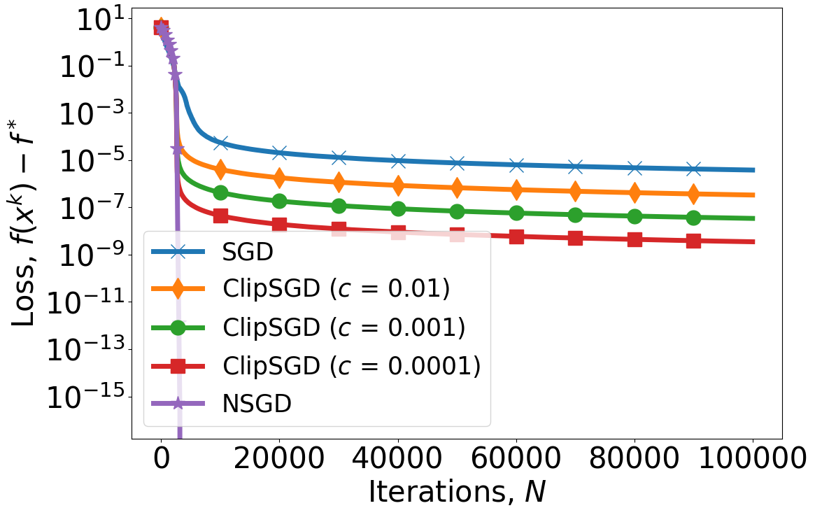
Figure 1: Comparison of convergence of SGD, NSGD and ClipSGD on w1a dataset $(B=1000)$

In Figure 1, we see that SGD (see Theorem 3.1) converges sublinearly, but using ClipSGD we can significantly improve the number of iterations to achieve the desired accuracy by varying $c$. However, if we take too small $c$, the convergence will be the same as NSGD, thus confirming our theoretical results.

8 Conclusion

In this paper, we considered a stochastic optimization problem assuming that the function is $(L_{0},L_{1})$-smooth. In Sections 3 and 4, we have shown in which regimes we can achieve linear convergence rate, thereby significantly improving all previous work. Moreover, we extend this advantage and show in Section 5 that zero-order algorithms can also achieve linear convergence rates in the convex setting. In addition, we show that generalized smoothness improves not only the iteration and oracle complexities, but also the maximum allowable noise level. We confirmed our results by numerical experiment of interest in the field of machine learning. Finally, we discussed future work, thereby showing that our work opens a series of directions for research.

Appendix A Auxiliary Results

In this section we provide auxiliary materials that are used in the proof of Theorems.

A.1 Basic inequalities and assumptions

Basic inequalities.

For all $a,b\in\mathbb{R}^{d}$ ($d\geq 1$) the following equality holds:

$$2\left\langle a,b\right\rangle-\|b\|^{2}=\|a\|^{2}-\|a-b\|^{2},$$ (5)

$$\left\langle a,b\right\rangle\leq\|a\|\cdot\|b\|.$$ (6)

Squared norm of the sum

For all $a_{1},...,a_{n}\in\mathbb{R}^{d}$, where $n=\{2,3\}$

$$\|a_{1}+...+a_{n}\|_{2}^{2}\leq n\|a_{1}\|_{2}^{2}+...+n\|a_{n}\|_{2}^{2}.$$ (7)

Generalized-Lipschitz-smoothness.

Throughout this paper, we assume that the $(L_{0},L_{1})$-smoothness condition (Assumption 1.2) is satisfied. This inequality can be represented in the equivalent form for any $x,y\in\mathbb{R}^{d}$:

$$f(y)-f(x)\leq\left\langle\nabla f(x),y-x\right\rangle+\frac{L_{0}+L_{1}\left\|\nabla f(x)\right\|}{2}\left\|y-x\right\|^{2},$$ (8)

where $L_{0},L_{1}\geq 0$ for any $x\in\mathbb{R}^{d}$ and $\left\|y-x\right\|\leq\frac{1}{L_{1}}$.

Variance decomposition.

If $\xi$ is random vector in $\mathbb{R}^{d}$ with bounded second moment, then

$$\mathbb{E}\left[\left\|\xi+a\right\|^{2}\right]=\mathbb{E}\left[\left\|\xi-\mathbb{E}\left[\xi\right]\right\|^{2}\right]+\mathbb{E}\left[\left\|\mathbb{E}\left[\xi\right]-a\right\|^{2}\right],$$ (9)

for any deterministic vector $a\in\mathbb{R}^{d}$.

A.2 Auxiliary Lemma about Generalized Smoothness

If Assumption 1.2 holds, then it also holds that $\forall x\in\mathbb{R}^{d}$:

$$\left\|\nabla f(x)\right\|^{2}\leq 2(L_{0}+L_{1}\left\|\nabla f(x)\right\|)(f(x)-f^{*}),$$ (10)

where $f^{*}=\inf_{x}f(x)$.

Proof.

We start the proof by applying (8) for $y=x-\frac{1}{L_{0}+L_{1}\left\|\nabla f(x)\right\|}\nabla f(x)$, where $\left\|y-x\right\|=\frac{\left\|\nabla f(x)\right\|}{L_{0}+L_{1}\left\|\nabla f(x)\right\|}\leq\frac{1}{L_{1}}$. Then we can obtain:

$$f^{*}\leq f\left(x-\frac{1}{L_{0}+L_{1}\left\|\nabla f(x)\right\|}\nabla f(x)\right)\overset{\eqref{eq:ass_smooth}}{\leq}f(x)-\frac{1}{2(L_{0}+L_{1}\left\|\nabla f(x)\right\|)}\left\|\nabla f(x)\right\|^{2}.$$

∎

A.3 Wirtinger-Poincare inequality

Let $f$ is differentiable, then for all $x\in\mathbb{R}^{d}$, $\gamma e\in S^{d}(\gamma)$:

$$\mathbb{E}\left[f(x+\gamma e)^{2}\right]\leq\frac{\gamma^{2}}{d}\mathbb{E}\left[\left\|\nabla f(x+\gamma e)\right\|^{2}\right].$$ (11)

Appendix B Stochastic Gradient Descent

B.1 SGD under Deterministic $(L_{0},L_{1})$-Smoothness (Assumption 1.2)

We start by using $(L_{0},L_{1})$-smoothness (see Assumption 1.2):

$$\mathbb{E}\left[f(x^{k+1})\right]-f(x^{k}) \overset{\eqref{eq:ass_smooth}}{\leq}\left\langle\nabla f(x^{k}),\mathbb{E}\left[x^{k+1}\right]-x^{k}\right\rangle+\frac{L_{0}+L_{1}\left\|\nabla f(x^{k})\right\|}{2}\mathbb{E}\left[\left\|x^{k+1}-x^{k}\right\|^{2}\right]$$

$$=-\eta\left\langle\nabla f(x^{k}),\mathbb{E}\left[\nabla f(x^{k},\bm{\xi}^{k})\right]\right\rangle+\frac{\eta^{2}(L_{0}+L_{1}\left\|\nabla f(x^{k})\right\|)}{2}\left\|\mathbb{E}\left[\nabla f(x^{k},\bm{\xi}^{k})\right]\right\|^{2}.$$ (12)

Let’s evaluate the first summand of (12)

$$-\eta\left\langle\nabla f(x^{k}),\mathbb{E}\left[\nabla f(x^{k},\bm{\xi}^{k})\right]\right\rangle =-\frac{\eta}{2}\left\|\nabla f(x^{k})\right\|^{2}-\frac{\eta}{2}\mathbb{E}\left[\left\|\nabla f(x^{k},\bm{\xi}^{k})\right\|^{2}\right]+\frac{\eta}{2}\mathbb{E}\left[\left\|\nabla f(x^{k},\bm{\xi}^{k})-\nabla f(x^{k})\right\|^{2}\right]$$

$$\leq-\frac{\eta}{2}\left\|\nabla f(x^{k})\right\|^{2}-\frac{\eta}{2}\mathbb{E}\left[\left\|\nabla f(x^{k},\bm{\xi}^{k})\right\|^{2}\right]+\frac{\eta\sigma^{2}}{2B}.$$

Plugging this into (12) and choosing $\eta\leq\frac{1}{L_{0}+L_{1}M}$ we have:

$$\mathbb{E}\left[f(x^{k+1})\right]-f(x^{k}) \overset{\eqref{eq:det_SGD_smooth}}{\leq}-\frac{\eta}{2}\left\|\nabla f(x^{k})\right\|^{2}-\frac{\eta}{2}\mathbb{E}\left[\left\|\nabla f(x^{k},\bm{\xi}^{k})\right\|^{2}\right]+\frac{\eta\sigma^{2}}{2B}$$

$$\quad\quad+\frac{\eta^{2}(L_{0}+L_{1}\left\|\nabla f(x^{k})\right\|)}{2}\mathbb{E}\left[\left\|\nabla f(x^{k},\bm{\xi}^{k})\right\|^{2}\right]$$

$$=-\frac{\eta}{2}\left\|\nabla f(x^{k})\right\|^{2}-\frac{\eta}{2}\mathbb{E}\left[\left\|\nabla f(x^{k},\bm{\xi}^{k})\right\|^{2}\right]\left(1-\eta(L_{0}+L_{1}M)\right)+\frac{\eta\sigma^{2}}{2B}$$

$$\leq-\frac{\eta}{2}\left\|\nabla f(x^{k})\right\|^{2}+\frac{\eta\sigma^{2}}{2B}.$$

Rearrange the summands, then we have

$$\left\|\nabla f(x^{k})\right\|^{2}\leq 2\frac{f(x^{k})-\mathbb{E}\left[f(x^{k+1})\right]}{\eta}+\sigma^{2}.$$ (13)

Let $r_{k+1}=\mathbb{E}\left[\left\|x^{k+1}-x^{*}\right\|\right]$ and $F_{k+1}=\mathbb{E}\left[f(x^{k+1})-f^{*}\right]$, then we get:

$$r_{k+1}^{2} =r_{k}^{2}-2\eta\left\langle\mathbb{E}\left[\nabla f(x^{k},\bm{\xi}^{k})\right],x^{k}-x^{*}\right\rangle+\eta^{2}\mathbb{E}\left[\left\|\nabla f(x^{k},\bm{\xi}^{k})\right\|^{2}\right]$$

$$\overset{\eqref{eq:Variance_decomposition}}{=}r_{k}^{2}-2\eta\left\langle\nabla f(x^{k}),x^{k}-x^{*}\right\rangle+\eta^{2}\mathbb{E}\left[\left\|\nabla f(x^{k},\bm{\xi}^{k})-\nabla f(x^{k})\right\|^{2}\right]+\eta^{2}\left\|\nabla f(x^{k})\right\|^{2}$$

$$\overset{\text{\char 172}}{\leq}r_{k}^{2}-2\eta F_{k}+\eta^{2}\mathbb{E}\left[\left\|\nabla f(x^{k},\bm{\xi}^{k})-\nabla f(x^{k})\right\|^{2}\right]+\eta^{2}\left\|\nabla f(x^{k})\right\|^{2}$$

$$\leq r_{k}^{2}-2\eta F_{k}+\eta^{2}\mathbb{E}\left[\left\|\nabla f(x^{k},\bm{\xi}^{k})-\nabla f(x^{k})\right\|^{2}\right]+\eta^{2}\left\|\nabla f(x^{k})\right\|^{2}$$

$$\leq r_{k}^{2}-2\eta F_{k}+\frac{2\eta^{2}\sigma^{2}}{B}+2\eta^{2}\left\|\nabla f(x^{k})\right\|^{2}$$

$$\overset{\eqref{det_SGD_case_2_norm_gradient}}{\leq}r_{k}^{2}-2\eta F_{k}+\frac{2\eta^{2}\sigma^{2}}{B}+2\eta F_{k}-2\eta F_{k+1}+\frac{2\eta^{2}\sigma^{2}}{B}$$

$$\leq r_{k}^{2}+\frac{4\eta^{2}\sigma^{2}}{B}-2\eta F_{k+1},$$

where in ① we use Assumption 1.3 with $\mu=0$.

Rearranging and summing over all $k=0,1,2,...,N-1$, we obtain

$$2\eta NF_{N}\leq 2\eta\sum_{k=0}^{N-1}F_{k+1}\leq\sum_{k=0}^{N-1}\left(r_{k}^{2}-r_{k+1}^{2}\right)+\sum_{k=0}^{N-1}\frac{4\eta^{2}\sigma^{2}}{B}=r_{0}^{2}-r_{N}^{2}+\frac{4\eta^{2}\sigma^{2}N}{B}\leq r_{0}^{2}+\frac{4\eta^{2}\sigma^{2}N}{B}.$$

Hence we obtain:

$$\mathbb{E}\left[f(x^{N})\right]-f^{*}\leq\frac{R^{2}}{2\eta N}+\frac{2\eta\sigma^{2}}{B}.$$

B.2 SGD under Stochastic $(L_{0},L_{1})$-Smoothness (Assumption 3.2)

We start by using $(L_{0},L_{1})$-smoothness (see Assumption 3.2):

$$f(x^{k+1},\xi^{k})-f(x^{k},\xi^{k}) \overset{\eqref{eq:ass_smooth}}{\leq}\left\langle\nabla f(x^{k},\xi^{k}),x^{k+1}\right\rangle-x^{k}+\frac{L_{0}+L_{1}\left\|\nabla f(x^{k},\xi^{k})\right\|}{2}\left\|x^{k+1}-x^{k}\right\|^{2}$$

$$=-\eta\left\langle\nabla f(x^{k},\xi^{k}),\nabla{f(x^{k},\xi^{k})}\right\rangle+\frac{\eta^{2}(L_{0}+L_{1}\left\|\nabla f(x^{k},\xi^{k})\right\|)}{2}\left\|\nabla f(x^{k},\xi^{k})\right\|^{2}.$$ (14)

Choosing $\eta=\frac{1}{L_{0}+L_{1}\left\|\nabla f(x^{k},\xi^{k})\right\|}$ we consider two cases:

• In the case $\left\|\nabla f(x^{k},\xi^{k})\right\|\geq\frac{L_{0}}{L_{1}}$ we have

  $$f(x^{k+1},\xi^{k})-f(x^{k},\xi^{k}) \overset{\eqref{eq:stoch_SGD_smooth}}{\leq}-\eta\left\|\nabla{f(x^{k},\xi^{k})}\right\|^{2}+\frac{\eta}{2}\left\|\nabla f(x^{k},\xi^{k})\right\|^{2}$$

  $$=-\frac{\eta}{2}\left\|\nabla f(x^{k},\xi^{k})\right\|^{2}$$

  $$\leq\frac{1}{4L_{1}}\left\|\nabla f(x^{k},\xi^{k})\right\|.$$ (15)

  Using the convexity assumption of the function (see Assumption 1.3, $\mu=0$), we have the following:

  $$f(x^{k},\xi^{k})-f(x^{*},\xi^{k}) \leq\left\langle\nabla f(x^{k},\xi^{k}),x^{k}-x^{*}\right\rangle$$

  $$\overset{\eqref{eq:scalar_product_bound}}{\leq}\left\|\nabla f(x^{k},\xi^{k})\right\|\left\|x^{k}-x^{*}\right\|$$

  $$\leq\left\|\nabla f(x^{k},\xi^{k})\right\|\underbrace{\left\|x^{0}-x^{*}\right\|}_{R}.$$

  Hence we have:

  $$\left\|\nabla f(x^{k},\xi^{k})\right\|\geq\frac{f(x^{k},\xi^{k})-f(x^{*},\xi^{k})}{R}.$$ (16)

  Then substituting (16) into (15) we obtain:

  $$\mathbb{E}\left[f(x^{k+1},\xi^{k})-f(x^{k},\xi^{k})\right]\leq-\frac{1}{4L_{1}}\mathbb{E}\left[\left\|\nabla f(x^{k},\xi^{k})\right\|\right]\leq-\frac{1}{4L_{1}R}\mathbb{E}\left[f(x^{k},\xi^{k})-f(x^{*},\xi^{k})\right].$$

  Rearrange the summands, then we have

  $$\mathbb{E}\left[f(x^{k+1})\right]-f^{*} \leq\left(1-\frac{1}{4L_{1}R}\right)(f(x^{k})-f^{*}).$$

  Let $\mathcal{T}_{1}=\left\{m^{\mathcal{T}_{1}}_{0},m^{\mathcal{T}_{1}}_{1},m^{\mathcal{T}_{1}}_{2},...,m^{\mathcal{T}_{1}}_{K-1}\right\}=\left\{k\in\{0,1,2,...,N-1\}|\left\|\nabla f(x^{k},\xi^{k})\right\|\geq\frac{L_{0}}{L_{1}}\right\}$, where $K=|\mathcal{T}_{1}|$. Then for $k\in\mathcal{T}_{1}$ SGD shows linear convergence:

  $$F_{N}\cdot\mathds{1}\left[\mathcal{T}_{1}\right]\leq\left(1-\frac{1}{4L_{1}R}\right)F_{N}\leq\left(1-\frac{1}{4L_{1}R}\right)F_{m^{\mathcal{T}_{1}}_{K-1}}\leq...\leq\left(1-\frac{1}{4L_{1}R}\right)^{K}F_{m_{0}^{\mathcal{T}_{1}}}\leq\left(1-\frac{1}{4L_{1}R}\right)^{K}F_{0},$$

  where $F_{k}=\mathbb{E}\left[f(x^{k})\right]-f^{*}$, and we used that $F_{k}\leq F_{k-1}$.

• In the case $\left\|\nabla f(x^{k},\xi^{k})\right\|<\frac{L_{0}}{L_{1}}$ we have

  $$f(x^{k+1},\xi^{k})-f(x^{k},\xi^{k}) \leq-\eta\left\|\nabla{f(x^{k},\xi^{k})}\right\|^{2}+\frac{\eta}{2}\left\|\nabla f(x^{k},\xi^{k})\right\|^{2}$$

  $$=-\frac{\eta}{2}\left\|\nabla f(x^{k},\xi^{k})\right\|^{2}.$$

  Rearrange the summands, then we have

  $$\mathbb{E}\left[\left\|\nabla f(x^{k},\xi^{k})\right\|^{2}\right]\leq 2\frac{f(x^{k})-\mathbb{E}\left[f(x^{k+1})\right]}{\eta}\leq\frac{f(x^{k})-\mathbb{E}\left[f(x^{k+1})\right]}{\eta}.$$

  Let $r_{k+1}=\mathbb{E}\left[\left\|x^{k+1}-x^{*}\right\|\right]$ and $F_{k+1}=\mathbb{E}\left[f(x^{k+1})-f^{*}\right]$, then we get:

  $$r_{k+1}^{2} =r_{k}^{2}-2\eta\left\langle\mathbb{E}\left[\nabla f(x^{k},\xi^{k})\right],x^{k}-x^{*}\right\rangle+\eta^{2}\mathbb{E}\left[\left\|\nabla f(x^{k},\xi^{k})\right\|^{2}\right]$$

  $$\leq r_{k}^{2}-2\eta F_{k}+2\eta F_{k}-2\eta F_{k+1}$$

  $$\leq r_{k}^{2}-2\eta F_{k+1}$$

  $$\leq r_{k}^{2}-\frac{F_{k+1}}{L_{0}}.$$

Let $\mathcal{T}_{2}=\left\{m^{\mathcal{T}_{2}}_{0},m^{\mathcal{T}_{2}}_{1},m^{\mathcal{T}_{2}}_{2},...,m^{\mathcal{T}_{2}}_{N-K}\right\}=\left\{k\in\{0,1,2,...,N-1\}|\left\|\nabla f(x^{k},\xi^{k})\right\|<\frac{L_{0}}{L_{1}}\right\}$, where $|\mathcal{T}_{2}|=N-K$. Then rearranging and summing over all $k\in\mathcal{T}_{2}$ we obtain

$$F_{N}\cdot\mathds{1}\left[\mathcal{T}_{2}\right]\leq\frac{1}{N-K+1}\sum_{k\in\mathcal{T}_{2}}F_{k+1}\leq\frac{L_{0}}{N-K+1}\sum_{k\in\mathcal{T}_{2}}\left(r_{k}^{2}-r_{k+1}^{2}\right)=\frac{L_{0}(r_{0}^{2}-r_{N}^{2})}{N-K}\leq\frac{L_{0}r_{0}^{2}}{N-K}.$$

Hence we obtain:

$$F_{N}\cdot\mathds{1}\left[\mathcal{T}_{2}\right]\leq\frac{L_{0}R^{2}}{N}.$$

Combining the two cases we have:

$$\mathbb{E}\left[f(x^{N})\right]-f^{*}\leq F_{N}\cdot\mathds{1}\left[\mathcal{T}_{1}\right]+F_{N}\cdot\mathds{1}\left[\mathcal{T}_{2}\right]\leq\left(1-\frac{1}{4L_{1}R}\right)^{K}(f(x^{0})-f^{*})+\frac{L_{0}R^{2}}{N-K}.$$

B.3 SGD under Strongly Convexity (Assumption 1.3, $\mu>0$)

We start by using $(L_{0},L_{1})$-smoothness (see Assumption 1.2):

$$\mathbb{E}\left[f(x^{k+1})\right]-f(x^{k}) \overset{\eqref{eq:ass_smooth}}{\leq}\left\langle\nabla f(x^{k}),\mathbb{E}\left[x^{k+1}\right]-x^{k}\right\rangle+\frac{L_{0}+L_{1}\left\|\nabla f(x^{k})\right\|}{2}\mathbb{E}\left[\left\|x^{k+1}-x^{k}\right\|^{2}\right]$$

$$=-\eta\left\langle\nabla f(x^{k}),\mathbb{E}\left[\nabla f(x^{k},\bm{\xi}^{k})\right]\right\rangle+\frac{\eta^{2}(L_{0}+L_{1}\left\|\nabla f(x^{k})\right\|)}{2}\left\|\mathbb{E}\left[\nabla f(x^{k},\bm{\xi}^{k})\right]\right\|^{2}.$$ (17)

Let’s evaluate the first summand of (17)

$$-\eta\left\langle\nabla f(x^{k}),\mathbb{E}\left[\nabla f(x^{k},\bm{\xi}^{k})\right]\right\rangle =-\frac{\eta}{2}\left\|\nabla f(x^{k})\right\|^{2}-\frac{\eta}{2}\mathbb{E}\left[\left\|\nabla f(x^{k},\bm{\xi}^{k})\right\|^{2}\right]+\frac{\eta}{2}\mathbb{E}\left[\left\|\nabla f(x^{k},\bm{\xi}^{k})-\nabla f(x^{k})\right\|^{2}\right]$$

$$\leq-\frac{\eta}{2}\left\|\nabla f(x^{k})\right\|^{2}-\frac{\eta}{2}\mathbb{E}\left[\left\|\nabla f(x^{k},\bm{\xi}^{k})\right\|^{2}\right]+\frac{\eta\sigma^{2}}{2B}.$$

Plugging this into (17) and choosing $\eta\leq\frac{1}{L_{0}+L_{1}M}$ we have:

$$\mathbb{E}\left[f(x^{k+1})\right]-f(x^{k}) \overset{\eqref{eq:Strongly_SGD_smooth}}{\leq}-\frac{\eta}{2}\left\|\nabla f(x^{k})\right\|^{2}-\frac{\eta}{2}\mathbb{E}\left[\left\|\nabla f(x^{k},\bm{\xi}^{k})\right\|^{2}\right]+\frac{\eta\sigma^{2}}{2B}$$

$$\quad\quad+\frac{\eta^{2}(L_{0}+L_{1}\left\|\nabla f(x^{k})\right\|)}{2}\mathbb{E}\left[\left\|\nabla f(x^{k},\bm{\xi}^{k})\right\|^{2}\right]$$

$$=-\frac{\eta}{2}\left\|\nabla f(x^{k})\right\|^{2}-\frac{\eta}{2}\mathbb{E}\left[\left\|\nabla f(x^{k},\bm{\xi}^{k})\right\|^{2}\right]\left(1-\eta(L_{0}+L_{1}M)\right)+\frac{\eta\sigma^{2}}{2B}$$

$$\leq-\frac{\eta}{2}\left\|\nabla f(x^{k})\right\|^{2}+\frac{\eta\sigma^{2}}{2B}.$$ (18)

Using the strongly convexity assumption of the function (see Assumption 1.3, $\mu>0$), we have the following:

$$f(x^{k})-f^{*} \leq\left\langle\nabla f(x^{k}),x^{k}-x^{*}\right\rangle-\frac{\mu}{2}\left\|x^{k}-x^{*}\right\|^{2}$$

$$=\frac{1}{2\mu}\left\|\nabla f(x^{k})\right\|^{2}-\left\|\sqrt{\frac{\mu}{2}}(x^{k}-x^{*})-\sqrt{\frac{1}{2\mu}}\nabla f(x^{k})\right\|^{2}$$

$$\leq\frac{1}{2\mu}\left\|\nabla f(x^{k})\right\|^{2}.$$

Hence we have:

$$\left\|\nabla f(x^{k})\right\|^{2}\geq 2\mu(f(x^{k})-f^{*}).$$ (19)

Then substituting (19) into (18) we obtain:

$$\mathbb{E}\left[f(x^{k+1})\right]-f(x^{k})\leq-\frac{\eta}{2}\left\|\nabla f(x^{k})\right\|^{2}+\frac{\eta\sigma^{2}}{2B}\leq-\eta\mu(f(x^{k},\xi^{k})-f^{*})+\frac{\eta\sigma^{2}}{2B}.$$

Rearrange the summands, then we have

$$\mathbb{E}\left[f(x^{k+1})\right]-f^{*} \leq\left(1-\eta\mu\right)(f(x^{k})-f^{*})+\frac{\eta\sigma^{2}}{2B}.$$

Then for $k=0,1,2,...,N-1$ iterations SGD shows linear convergence:

$$\mathbb{E}\left[f(x^{N})\right]-f^{*}\leq\left(1-\eta\mu\right)^{N}(f(x^{0})-f^{*})+\frac{\sigma^{2}}{2\mu B}.$$

Appendix C Normalized Stochastic Gradient Descent

Let’s introduce the notation $G(x^{k},\bm{\xi}^{k})=\frac{\nabla f(x^{k},\bm{\xi}^{k})}{\left\|\nabla f(x^{k},\bm{\xi}^{k})\right\|}$, then using $(L_{0},L_{1})$-smoothness (see Assumption 1.2):

$$f(x^{k+1})-f(x^{k}) \overset{\eqref{eq:ass_smooth}}{\leq}\left\langle\nabla f(x^{k}),x^{k+1}-x^{k}\right\rangle+\frac{L_{0}+L_{1}\left\|\nabla f(x^{k})\right\|}{2}\left\|x^{k+1}-x^{k}\right\|^{2}$$

$$=-\eta\left\langle\nabla f(x^{k}),G(x^{k},\bm{\xi}^{k})\right\rangle+\frac{\eta^{2}(L_{0}+L_{1}\left\|\nabla f(x^{k})\right\|)}{2}\left\|G(x^{k},\bm{\xi}^{k})\right\|^{2}.$$ (20)

Next, we consider 4 cases of the relation $\left\|\nabla f(x^{k})\right\|$ and $\left\|\nabla f(x^{k},\bm{\xi}^{k})\right\|$ with respect to the hyperparameter $\lambda$.

C.1 First case: $\left\|\nabla f(x^{k})\right\|\geq\lambda$ and $\|\nabla f(x^{k},\bm{\xi}^{k})\|\geq\lambda$

Let us evaluate first summand of (20) with $\alpha=\left\|\nabla f(x^{k})\right\|^{-1}$:

$$-\eta\left\langle\nabla f(x^{k}),G(x^{k},\bm{\xi}^{k})\right\rangle \overset{\eqref{eq:qudrat_raznosti}}{=}-\frac{\alpha\eta}{2}\left\|\nabla f(x^{k})\right\|^{2}-\frac{\eta}{2\alpha}\left\|G(x^{k},\bm{\xi}^{k})\right\|^{2}+\frac{\eta}{2\alpha}\left\|G(x^{k},\bm{\xi}^{k})-\alpha\nabla f(x^{k})\right\|^{2}$$

$$=-\frac{\eta}{2}\left\|\nabla f(x^{k})\right\|-\frac{\eta}{2\alpha}\left\|G(x^{k},\bm{\xi}^{k})\right\|^{2}+\frac{\eta}{2\lambda^{2}\alpha}\left\|\lambda G(x^{k},\bm{\xi}^{k})-\lambda\alpha\nabla f(x^{k})\right\|^{2}$$

$$=-\frac{\eta}{2}\left\|\nabla f(x^{k})\right\|-\frac{\eta}{2\alpha}\left\|G(x^{k},\bm{\xi}^{k})\right\|^{2}+\frac{\eta}{2\lambda^{2}\alpha}\left\|\text{clip}_{\lambda}\left(\nabla f(x^{k},\bm{\xi}^{k})\right)-\text{clip}_{\lambda}\left(\nabla f(x^{k})\right)\right\|^{2}$$

Using that clipping is a projection on onto a convex set, namely ball with radius $\lambda$, and thus is Lipshitz operator with Lipshitz constant $1$, we can obtain:

$$-\eta\left\langle\nabla f(x^{k}),\mathbb{E}\left[G(x^{k},\bm{\xi}^{k})\right]\right\rangle \leq-\frac{\eta}{2}\left\|\nabla f(x^{k})\right\|-\frac{\eta}{2\alpha}\mathbb{E}\left[\left\|G(x^{k},\bm{\xi}^{k})\right\|^{2}\right]+\frac{\eta}{2\lambda^{2}\alpha}\mathbb{E}\left[\left\|\nabla f(x^{k},\bm{\xi}^{k})-\nabla f(x^{k})\right\|^{2}\right].$$ (21)

In the case: $0\leq\sigma\leq\frac{\lambda}{\sqrt{2}}$.

Using this in (21), we have the following with $\eta_{k}\leq\frac{\left\|\nabla f(x^{k})\right\|}{2(L_{0}+L_{1}\left\|\nabla f(x^{k})\right\|)}$:

$$\mathbb{E}\left[f(x^{k+1})\right]-f(x^{k}) \overset{\eqref{eq:NSGD_smooth}}{\leq}-\eta\left\langle\nabla f(x^{k}),\mathbb{E}\left[G(x^{k},\bm{\xi}^{k})\right]\right\rangle+\frac{\eta^{2}(L_{0}+L_{1}\left\|\nabla f(x^{k})\right\|)}{2}\mathbb{E}\left[\left\|G(x^{k},\bm{\xi}^{k})\right\|^{2}\right]$$

$$\overset{\eqref{eq:NSGD1_main}}{\leq}-\frac{\eta}{2}\left\|\nabla f(x^{k})\right\|-\frac{\eta}{2\alpha}\mathbb{E}\left[\left\|G(x^{k},\bm{\xi}^{k})\right\|^{2}\right]+\frac{\eta}{2\lambda^{2}\alpha}\mathbb{E}\left[\left\|\nabla f(x^{k},\bm{\xi})-\nabla f(x^{k})\right\|^{2}\right]$$

$$\quad\quad\quad+\frac{\eta^{2}(L_{0}+L_{1}\left\|\nabla f(x^{k})\right\|)}{2}\mathbb{E}\left[\left\|G(x^{k},\bm{\xi}^{k})\right\|^{2}\right]$$

$$=-\frac{\eta}{2}\left\|\nabla f(x^{k})\right\|+\frac{\eta}{2\lambda^{2}\alpha}\mathbb{E}\left[\left\|\nabla f(x^{k},\bm{\xi}^{k})-\nabla f(x^{k})\right\|^{2}\right]$$

$$\quad\quad\quad-\frac{\eta}{2}\mathbb{E}\left[\left\|G(x^{k},\bm{\xi}^{k})\right\|^{2}\right]\left(1-\frac{\eta(L_{0}+L_{1}\left\|\nabla f(x^{k})\right\|)}{\left\|\nabla f(x^{k})\right\|}\right)$$

$$\leq-\frac{\eta}{2}\left\|\nabla f(x^{k})\right\|+\frac{\eta\sigma^{2}}{2\lambda^{2}\alpha}$$

$$\leq-\frac{\eta}{2}\left\|\nabla f(x^{k})\right\|+\frac{\eta}{4}\left\|\nabla f(x^{k})\right\|$$

$$=-\frac{\eta}{4}\left\|\nabla f(x^{k})\right\|.$$ (22)

The step size will be constant, depending on the hyperparameter $\lambda$:

$$\frac{\left\|\nabla f(x^{k})\right\|}{2\left(L_{0}+L_{1}\left\|\nabla f(x^{k})\right\|\right)}=\frac{1}{2\left(L_{0}\frac{1}{\left\|\nabla f(x^{k})\right\|}+L_{1}\right)}=\frac{\lambda}{2\left(L_{0}\frac{\lambda}{\left\|\nabla f(x^{k})\right\|}+L_{1}\lambda\right)}\geq\frac{\lambda}{2\left(L_{0}+L_{1}\lambda\right)}.$$

Thus, $\eta_{k}=\eta\leq\frac{\lambda}{2(L_{0}+L_{1}\lambda)}$.

Using the convexity assumption of the function (see Assumption 1.3, $\mu=0$), we have the following:

$$f(x^{k})-f^{*} \leq\left\langle\nabla f(x^{k}),x^{k}-x^{*}\right\rangle$$

$$\overset{\eqref{eq:scalar_product_bound}}{\leq}\left\|\nabla f(x^{k})\right\|\left\|x^{k}-x^{*}\right\|$$

$$\leq\left\|\nabla f(x^{k})\right\|\underbrace{\left\|x^{0}-x^{*}\right\|}_{R}.$$

Hence we have:

$$\left\|\nabla f(x^{k})\right\|\geq\frac{f(x^{k})-f^{*}}{R}.$$ (23)

Then substituting (23) into (22) we obtain:

$$\mathbb{E}\left[f(x^{k+1})\right]-f(x^{k})\leq-\frac{\eta}{4}\left\|\nabla f(x^{k})\right\|\leq-\frac{\eta}{4R}(f(x^{k})-f^{*}).$$

This inequality is equivalent to the trailing inequality:

$$\mathbb{E}\left[f(x^{k+1})\right]-f^{*}\leq\left(1-\frac{\eta}{4R}\right)\left(f(x^{k})-f^{*}\right).$$

Then for $k=0,1,2,...,N-1$ iterations that satisfy the conditions $\left\|\nabla f(x^{k},\bm{\xi}^{k})\right\|\geq\sqrt{2}\sigma$ and $\left\|\nabla f(x^{k})\right\|\geq\sqrt{2}\sigma$ NSGD shows linear convergence:

$$\mathbb{E}\left[f(x^{N})\right]-f^{*}\leq\left(1-\frac{\eta}{4R}\right)^{N}(f(x^{0})-f^{*}).$$

In the case: $\frac{\lambda}{\sqrt{2}}\leq\sigma$.

Using this in (21), we have the following with $\eta_{k}\leq\frac{\left\|\nabla f(x^{k})\right\|}{2(L_{0}+L_{1}\left\|\nabla f(x^{k})\right\|)}$:

$$\mathbb{E}\left[f(x^{k+1})\right]-f(x^{k}) \overset{\eqref{eq:NSGD_smooth}}{\leq}-\eta\left\langle\nabla f(x^{k}),\mathbb{E}\left[G(x^{k},\bm{\xi}^{k})\right]\right\rangle+\frac{\eta^{2}(L_{0}+L_{1}\left\|\nabla f(x^{k})\right\|)}{2}\mathbb{E}\left[\left\|G(x^{k},\bm{\xi}^{k})\right\|^{2}\right]$$

$$\overset{\eqref{eq:NSGD1_main}}{\leq}-\frac{\eta}{2}\left\|\nabla f(x^{k})\right\|-\frac{\eta}{2\alpha}\mathbb{E}\left[\left\|G(x^{k},\bm{\xi}^{k})\right\|^{2}\right]+\frac{\eta}{2\lambda^{2}\alpha}\mathbb{E}\left[\left\|\nabla f(x^{k},\bm{\xi}^{k})-\nabla f(x^{k})\right\|^{2}\right]$$

$$\quad\quad\quad+\frac{\eta^{2}(L_{0}+L_{1}\left\|\nabla f(x^{k})\right\|)}{2}\mathbb{E}\left[\left\|G(x^{k},\bm{\xi}^{k})\right\|^{2}\right]$$

$$=-\frac{\eta}{2}\left\|\nabla f(x^{k})\right\|+\frac{\eta}{2\lambda^{2}\alpha}\mathbb{E}\left[\left\|\nabla f(x^{k},\bm{\xi}^{k})-\nabla f(x^{k})\right\|^{2}\right]$$

$$\quad\quad\quad-\frac{\eta}{2}\mathbb{E}\left[\left\|G(x^{k},\bm{\xi}^{k})\right\|^{2}\right]\left(1-\frac{\eta(L_{0}+L_{1}\left\|\nabla f(x^{k})\right\|)}{\left\|\nabla f(x^{k})\right\|}\right)$$

$$\leq-\frac{\eta}{2}\left\|\nabla f(x^{k})\right\|+\frac{\eta\sigma^{2}}{2\lambda^{2}\alpha B}$$

$$\leq-\frac{\eta}{2}\left\|\nabla f(x^{k})\right\|+\frac{\eta\sigma^{2}M}{2\lambda^{2}B}.$$ (24)

The step size will be constant, depending on the hyperparameter $\lambda$:

$$\frac{\left\|\nabla f(x^{k})\right\|}{2\left(L_{0}+L_{1}\left\|\nabla f(x^{k})\right\|\right)}=\frac{1}{2\left(L_{0}\frac{1}{\left\|\nabla f(x^{k})\right\|}+L_{1}\right)}=\frac{\lambda}{2\left(L_{0}\frac{\lambda}{\left\|\nabla f(x^{k})\right\|}+L_{1}\lambda\right)}\geq\frac{\lambda}{2\left(L_{0}+L_{1}\lambda\right)}.$$

Thus, $\eta_{k}=\eta\leq\frac{\lambda}{2(L_{0}+L_{1}\lambda)}$.

Using the convexity assumption of the function (see Assumption 1.3, $\mu=0$), we have the following:

$$f(x^{k})-f^{*} \leq\left\langle\nabla f(x^{k}),x^{k}-x^{*}\right\rangle$$

$$\overset{\eqref{eq:scalar_product_bound}}{\leq}\left\|\nabla f(x^{k})\right\|\left\|x^{k}-x^{*}\right\|$$

$$\leq\left\|\nabla f(x^{k})\right\|\underbrace{\left\|x^{0}-x^{*}\right\|}_{R}.$$

Hence we have:

$$\left\|\nabla f(x^{k})\right\|\geq\frac{f(x^{k})-f^{*}}{R}.$$ (25)

Then substituting (25) into (24) we obtain:

$$\mathbb{E}\left[f(x^{k+1})\right]-f(x^{k})\leq-\frac{\eta}{2}\left\|\nabla f(x^{k})\right\|+\frac{\eta\sigma^{2}M}{2\lambda^{2}B}\leq-\frac{\eta}{2R}(f(x^{k})-f^{*})+\frac{\eta\sigma^{2}M}{2\lambda^{2}B}.$$

This inequality is equivalent to the trailing inequality:

$$\mathbb{E}\left[f(x^{k+1})\right]-f^{*}\leq\left(1-\frac{\eta}{2R}\right)\left(f(x^{k})-f^{*}\right)+\frac{\eta\sigma^{2}M}{2\lambda^{2}B}.$$

Then for $k=0,1,2,...,N-1$ iterations that satisfy the conditions $\left\|\nabla f(x^{k},\bm{\xi}^{k})\right\|\geq\lambda$ and $\left\|\nabla f(x^{k})\right\|\geq\lambda$ and $\sigma\geq\sqrt{2}\lambda$ NSGD shows linear convergence:

$$\mathbb{E}\left[f(x^{N})\right]-f^{*}\leq\left(1-\frac{\eta}{2R}\right)^{N}(f(x^{0})-f^{*})+\frac{\sigma^{2}MR}{\lambda^{2}B}.$$

C.2 Second case: $\left\|\nabla f(x^{k})\right\|\leq\lambda$ and $\left\|\nabla f(x^{k},\bm{\xi}^{k})\right\|\geq\lambda$

Let us evaluate first summand of (20) with $\alpha=\lambda^{-1}$:

$$-\eta\left\langle\nabla f(x^{k}),G(x^{k},\bm{\xi}^{k})\right\rangle \overset{\eqref{eq:qudrat_raznosti}}{=}-\frac{\alpha\eta}{2}\left\|\nabla f(x^{k})\right\|^{2}-\frac{\eta}{2\alpha}\left\|G(x^{k},\bm{\xi}^{k})\right\|^{2}+\frac{\eta}{2\alpha}\left\|G(x^{k},\bm{\xi}^{k})-\alpha\nabla f(x^{k})\right\|^{2}$$

$$\leq-\frac{\eta}{2}\left\|\nabla f(x^{k})\right\|-\frac{\eta}{2\alpha}\left\|G(x^{k},\bm{\xi}^{k})\right\|^{2}+\frac{\eta}{2\lambda}\left\|\lambda G(x^{k},\bm{\xi}^{k})-\nabla f(x^{k})\right\|^{2}$$

$$=-\frac{\eta}{2}\left\|\nabla f(x^{k})\right\|-\frac{\eta}{2\alpha}\left\|G(x^{k},\bm{\xi}^{k})\right\|^{2}+\frac{\eta}{2\lambda}\left\|\text{clip}_{\lambda}\left(\nabla f(x^{k},\bm{\xi}^{k})\right)-\text{clip}_{\lambda}\left(\nabla f(x^{k})\right)\right\|^{2}$$

Using that clipping is a projection on onto a convex set, namely ball with radius $\lambda$, and thus is Lipshitz operator with Lipshitz constant $1$, we can obtain:

$$-\eta\left\langle\nabla f(x^{k}),\mathbb{E}\left[G(x^{k},\bm{\xi}^{k})\right]\right\rangle \leq-\frac{\eta}{2}\left\|\nabla f(x^{k})\right\|-\frac{\eta}{2\alpha}\mathbb{E}\left[\left\|G(x^{k},\bm{\xi}^{k})\right\|^{2}\right]+\frac{\eta}{2\lambda}\mathbb{E}\left[\left\|\nabla f(x^{k},\bm{\xi}^{k})-\nabla f(x^{k})\right\|^{2}\right].$$ (26)

Using this, we have the following with $\eta_{k}\leq\frac{\left\|\nabla f(x^{k})\right\|}{2(L_{0}+L_{1}\left\|\nabla f(x^{k})\right\|)}$:

$$\mathbb{E}\left[f(x^{k+1})\right]-f(x^{k}) \overset{\eqref{eq:NSGD_smooth}}{\leq}-\eta\left\langle\nabla f(x^{k}),\mathbb{E}\left[G(x^{k},\bm{\xi}^{k})\right]\right\rangle+\frac{\eta^{2}(L_{0}+L_{1}\left\|\nabla f(x^{k})\right\|)}{2}\mathbb{E}\left[\left\|G(x^{k},\bm{\xi}^{k})\right\|^{2}\right]$$

$$\overset{\eqref{eq:NSGD2_main}}{\leq}-\frac{\eta}{2}\left\|\nabla f(x^{k})\right\|-\frac{\eta}{2\alpha}\mathbb{E}\left[\left\|G(x^{k},\bm{\xi}^{k})\right\|^{2}\right]+\frac{\eta}{2\lambda}\mathbb{E}\left[\left\|\nabla f(x^{k},\bm{\xi}^{k})-\nabla f(x^{k})\right\|^{2}\right]$$

$$\quad\quad\quad+\frac{\eta^{2}(L_{0}+L_{1}\left\|\nabla f(x^{k})\right\|)}{2}\mathbb{E}\left[\left\|G(x^{k},\bm{\xi}^{k})\right\|^{2}\right]$$

$$=-\frac{\eta}{2}\left\|\nabla f(x^{k})\right\|+\frac{\eta}{2\lambda}\mathbb{E}\left[\left\|\nabla f(x^{k},\bm{\xi}^{k})-\nabla f(x^{k})\right\|^{2}\right]$$

$$\quad\quad\quad-\frac{\eta}{2}\mathbb{E}\left[\left\|G(x^{k},\bm{\xi}^{k})\right\|^{2}\right]\left(1-\frac{\eta(L_{0}+L_{1}\left\|\nabla f(x^{k})\right\|)}{\left\|\nabla f(x^{k})\right\|}\right)$$

$$\leq-\frac{\eta}{2}\left\|\nabla f(x^{k})\right\|+\frac{\eta\sigma^{2}}{2\lambda B}$$

$$\leq-\frac{\eta}{2}\left\|\nabla f(x^{k})\right\|+\frac{\eta\sigma^{2}}{2\lambda B}.$$ (27)

The step size will be constant, depending on the hyperparameter $\lambda$:

$$\frac{\left\|\nabla f(x^{k})\right\|}{2\left(L_{0}+L_{1}\left\|\nabla f(x^{k})\right\|\right)}=\frac{1}{2\left(L_{0}\frac{1}{\left\|\nabla f(x^{k})\right\|}+L_{1}\right)}=\frac{\lambda}{2\left(L_{0}\frac{\lambda}{\left\|\nabla f(x^{k})\right\|}+L_{1}\lambda\right)}\geq\frac{\lambda}{2\left(L_{0}+L_{1}\lambda\right)}.$$

Thus, $\eta_{k}=\eta\leq\frac{\lambda}{2(L_{0}+L_{1}\lambda)}$.

Using the convexity assumption of the function (see Assumption 1.3, $\mu=0$), we have the following:

$$f(x^{k})-f^{*} \leq\left\langle\nabla f(x^{k}),x^{k}-x^{*}\right\rangle$$

$$\overset{\eqref{eq:scalar_product_bound}}{\leq}\left\|\nabla f(x^{k})\right\|\left\|x^{k}-x^{*}\right\|$$

$$\leq\left\|\nabla f(x^{k})\right\|\underbrace{\left\|x^{0}-x^{*}\right\|}_{R}.$$

Hence we have:

$$\left\|\nabla f(x^{k})\right\|\geq\frac{f(x^{k})-f^{*}}{R}.$$ (28)

Then substituting (28) into (27) we obtain:

$$\mathbb{E}\left[f(x^{k+1})\right]-f(x^{k})\leq-\frac{\eta}{2}\left\|\nabla f(x^{k})\right\|+\frac{\eta\sigma^{2}}{2\lambda B}\leq-\frac{\eta}{2R}(f(x^{k})-f^{*})+\frac{\eta\sigma^{2}}{2\lambda B}.$$

This inequality is equivalent to the trailing inequality:

$$\mathbb{E}\left[f(x^{k+1})\right]-f^{*}\leq\left(1-\frac{\eta}{2R}\right)\left(f(x^{k})-f^{*}\right)+\frac{\eta\sigma^{2}}{2\lambda B}.$$

Then for $k=0,1,2,...,N-1$ iterations that satisfy the conditions $\left\|\nabla f(x^{k})\right\|\leq\lambda$ and $\left\|\nabla f(x^{k},\bm{\xi}^{k})\right\|\geq\lambda$ NSGD shows linear convergence:

$$\mathbb{E}\left[f(x^{N})\right]-f^{*}\leq\left(1-\frac{\eta}{2R}\right)^{N}(f(x^{0})-f^{*})+\frac{\sigma^{2}R}{\lambda B}.$$

C.3 Third case: $\left\|\nabla f(x^{k})\right\|\leq\lambda$ and $\left\|\nabla f(x^{k},\bm{\xi}^{k})\right\|\leq\lambda$

Using this in (20), we have the following with $\eta_{k}\leq\frac{\left\|\nabla f(x^{k})\right\|}{2(L_{0}+L_{1}\left\|\nabla f(x^{k})\right\|)}$ and $\alpha=\left\|\nabla f(x^{k})\right\|^{-1}$:

$$\mathbb{E}\left[f(x^{k+1})\right]-f(x^{k}) \overset{\eqref{eq:NSGD_smooth}}{\leq}-\eta\left\langle\nabla f(x^{k}),\mathbb{E}\left[G(x^{k},\bm{\xi}^{k})\right]\right\rangle+\frac{\eta^{2}(L_{0}+L_{1}\left\|\nabla f(x^{k})\right\|)}{2}\mathbb{E}\left[\left\|G(x^{k},\bm{\xi}^{k})\right\|^{2}\right]$$

$$=-\frac{\eta\alpha}{2}\left\|\nabla f(x^{k})\right\|^{2}-\frac{\eta}{2\alpha}\mathbb{E}\left[\left\|G(x^{k},\bm{\xi}^{k})\right\|^{2}\right]+\frac{\eta}{2\alpha}\mathbb{E}\left[\left\|G(x^{k},\bm{\xi}^{k})-\alpha\nabla f(x^{k})\right\|^{2}\right]$$

$$\quad\quad\quad+\frac{\eta^{2}(L_{0}+L_{1}\left\|\nabla f(x^{k})\right\|)}{2}\mathbb{E}\left[\left\|G(x^{k},\bm{\xi}^{k})\right\|^{2}\right]$$

$$=-\frac{\eta}{2}\left\|\nabla f(x^{k})\right\|+\frac{\eta}{2\alpha}\mathbb{E}\left[\left\|G(x^{k},\bm{\xi}^{k})-\alpha\nabla f(x^{k})\right\|^{2}\right]$$

$$\quad\quad\quad-\frac{\eta}{2}\mathbb{E}\left[\left\|G(x^{k},\bm{\xi}^{k})\right\|^{2}\right]\left(1-\frac{\eta(L_{0}+L_{1}\left\|\nabla f(x^{k})\right\|)}{\left\|\nabla f(x^{k})\right\|}\right)$$

$$\leq-\frac{\eta}{2}\left\|\nabla f(x^{k})\right\|+\frac{\eta}{2\alpha}\mathbb{E}\left[\left\|G(x^{k},\bm{\xi}^{k})-\alpha\nabla f(x^{k})\right\|^{2}\right]$$

$$\leq-\frac{\eta}{2}\left\|\nabla f(x^{k})\right\|+\frac{\eta}{\alpha}\mathbb{E}\left[\left\|G(x^{k},\bm{\xi}^{k})\right\|^{2}+\left\|\alpha\nabla f(x^{k})\right\|^{2}\right]$$

$$=-\frac{\eta}{2}\left\|\nabla f(x^{k})\right\|+\frac{\eta}{\alpha}\mathbb{E}\left[\left\|\frac{\nabla f(x^{k},\bm{\xi}^{k})}{\left\|\nabla f(x^{k},\bm{\xi}^{k})\right\|}\right\|^{2}+\left\|\frac{\nabla f(x^{k})}{\left\|\nabla f(x^{k})\right\|}\right\|^{2}\right]$$

$$=-\frac{\eta}{2}\left\|\nabla f(x^{k})\right\|+\frac{2\eta\lambda\left\|\nabla f(x^{k})\right\|}{\lambda}$$

$$\leq-\frac{\eta}{2}\left\|\nabla f(x^{k})\right\|+2\eta\lambda.$$ (29)

The step size will be constant, depending on the hyperparameter $\lambda$:

$$\frac{\left\|\nabla f(x^{k})\right\|}{2\left(L_{0}+L_{1}\left\|\nabla f(x^{k})\right\|\right)}=\frac{1}{2\left(L_{0}\frac{1}{\left\|\nabla f(x^{k})\right\|}+L_{1}\right)}=\frac{\lambda}{2\left(L_{0}\frac{\lambda}{\left\|\nabla f(x^{k})\right\|}+L_{1}\lambda\right)}\geq\frac{\lambda}{2\left(L_{0}+L_{1}\lambda\right)}.$$

Thus, $\eta_{k}=\eta\leq\frac{\lambda}{2(L_{0}+L_{1}\lambda)}$.

Using the convexity assumption of the function (see Assumption 1.3, $\mu=0$), we have the following:

$$f(x^{k})-f^{*} \leq\left\langle\nabla f(x^{k}),x^{k}-x^{*}\right\rangle$$

$$\overset{\eqref{eq:scalar_product_bound}}{\leq}\left\|\nabla f(x^{k})\right\|\left\|x^{k}-x^{*}\right\|$$

$$\leq\left\|\nabla f(x^{k})\right\|\underbrace{\left\|x^{0}-x^{*}\right\|}_{R}.$$

Hence we have:

$$\left\|\nabla f(x^{k})\right\|\geq\frac{f(x^{k})-f^{*}}{R}.$$ (30)

Then substituting (30) into (29) we obtain:

$$\mathbb{E}\left[f(x^{k+1})\right]-f(x^{k})\leq-\frac{\eta}{2}\left\|\nabla f(x^{k})\right\|+2\eta\lambda\leq-\frac{\eta}{2R}(f(x^{k})-f^{*})+2\eta\lambda.$$

This inequality is equivalent to the trailing inequality:

$$\mathbb{E}\left[f(x^{k+1})\right]-f^{*}\leq\left(1-\frac{\eta}{2R}\right)\left(f(x^{k})-f^{*}\right)+2\eta\lambda.$$

Then for $k=0,1,2,...,N-1$ iterations that satisfy the conditions $\left\|\nabla f(x^{k})\right\|\leq\lambda$ NSGD shows linear convergence:

$$\mathbb{E}\left[f(x^{N})\right]-f^{*}\leq\left(1-\frac{\eta}{2R}\right)^{N}(f(x^{0})-f^{*})+\lambda R.$$

C.4 Fourth case: $\left\|\nabla f(x^{k})\right\|\geq\lambda$ and $\left\|\nabla f(x^{k},\bm{\xi}^{k})\right\|\leq\lambda$

Using this in (20), we have the following with $\eta_{k}\leq\frac{\left\|\nabla f(x^{k})\right\|}{2(L_{0}+L_{1}\left\|\nabla f(x^{k})\right\|)}$ and $\alpha=\lambda^{-1}$:

$$\mathbb{E}\left[f(x^{k+1})\right]-f(x^{k}) \overset{\eqref{eq:NSGD_smooth}}{\leq}-\eta\left\langle\nabla f(x^{k}),\mathbb{E}\left[G(x^{k},\bm{\xi}^{k})\right]\right\rangle+\frac{\eta^{2}(L_{0}+L_{1}\left\|\nabla f(x^{k})\right\|)}{2}\mathbb{E}\left[\left\|G(x^{k},\bm{\xi}^{k})\right\|^{2}\right]$$

$$=-\frac{\eta\alpha}{2}\left\|\nabla f(x^{k})\right\|^{2}-\frac{\eta}{2\alpha}\left\|\mathbb{E}\left[G(x^{k},\bm{\xi}^{k})\right]\right\|^{2}+\frac{\eta}{2\alpha}\left\|\mathbb{E}\left[G(x^{k},\bm{\xi}^{k})\right]-\alpha\nabla f(x^{k})\right\|^{2}$$

$$\quad\quad\quad+\frac{\eta^{2}(L_{0}+L_{1}\left\|\nabla f(x^{k})\right\|)}{2}\mathbb{E}\left[\left\|G(x^{k},\bm{\xi}^{k})\right\|^{2}\right]$$

$$=-\frac{\eta}{2\lambda}\left\|\nabla f(x^{k})\right\|^{2}+\frac{\eta}{2\lambda}\left\|\mathbb{E}\left[\lambda G(x^{k},\bm{\xi}^{k})\right]-\nabla f(x^{k})\right\|^{2}+\frac{\eta^{2}(L_{0}+L_{1}\left\|\nabla f(x^{k})\right\|)}{2}$$

$$=-\frac{\eta}{2\lambda}\left\|\nabla f(x^{k})\right\|^{2}+\frac{\eta}{2\lambda}\left\|\mathbb{E}\left[\frac{\lambda\nabla f(x^{k},\bm{\xi}^{k})}{\left\|\nabla f(x^{k},\bm{\xi}^{k})\right\|}-\nabla f(x^{k},\bm{\xi}^{k})\right]\right\|^{2}+\frac{\eta^{2}(L_{0}+L_{1}\left\|\nabla f(x^{k})\right\|)}{2}$$

$$=-\frac{\eta}{2\lambda}\left\|\nabla f(x^{k})\right\|^{2}+\frac{\eta}{2\lambda}\left\|\mathbb{E}\left[\left(\frac{\lambda}{\left\|\nabla f(x^{k},\bm{\xi}^{k})\right\|}-1\right)\nabla f(x^{k},\bm{\xi}^{k})\right]\right\|^{2}+\frac{\eta^{2}(L_{0}+L_{1}\left\|\nabla f(x^{k})\right\|)}{2}$$

$$\leq-\frac{\eta}{2\lambda}\left\|\nabla f(x^{k})\right\|^{2}+\frac{\eta}{2\lambda}\mathbb{E}\left[\left(\frac{\lambda}{\left\|\nabla f(x^{k},\bm{\xi}^{k})\right\|}-1\right)^{2}\left\|\nabla f(x^{k},\bm{\xi}^{k})\right\|^{2}\right]+\frac{\eta^{2}(L_{0}+L_{1}\left\|\nabla f(x^{k})\right\|)}{2}$$

$$\leq-\frac{\eta}{2\lambda}\left\|\nabla f(x^{k})\right\|^{2}+\frac{\eta}{2\lambda}\mathbb{E}\left[\frac{\lambda^{2}}{\left\|\nabla f(x^{k},\bm{\xi}^{k})\right\|^{2}}\left\|\nabla f(x^{k},\bm{\xi}^{k})\right\|^{2}\right]+\frac{\eta^{2}(L_{0}+L_{1}\left\|\nabla f(x^{k})\right\|)}{2}$$

$$=-\frac{\eta}{2\lambda}\left\|\nabla f(x^{k})\right\|^{2}+\frac{\eta^{2}(L_{0}+L_{1}\left\|\nabla f(x^{k})\right\|)}{2}+\frac{\eta\lambda}{2}$$

$$\leq-\frac{\eta}{2}\left\|\nabla f(x^{k})\right\|+\frac{\eta^{2}(L_{0}+L_{1}\left\|\nabla f(x^{k})\right\|)}{2}+\frac{\eta\lambda}{2}$$

$$=-\frac{\eta}{2}\left\|\nabla f(x^{k})\right\|\left(1-\frac{\eta(L_{0}+L_{1}\left\|\nabla f(x^{k})\right\|)}{\left\|\nabla f(x^{k})\right\|}\right)+\frac{\eta\lambda}{2}$$

$$\leq-\frac{\eta}{4}\left\|\nabla f(x^{k})\right\|+\frac{\eta\lambda}{2}.$$ (31)

The step size will be constant, depending on the hyperparameter $\lambda$:

$$\frac{\left\|\nabla f(x^{k})\right\|}{2\left(L_{0}+L_{1}\left\|\nabla f(x^{k})\right\|\right)}=\frac{1}{2\left(L_{0}\frac{1}{\left\|\nabla f(x^{k})\right\|}+L_{1}\right)}=\frac{\lambda}{2\left(L_{0}\frac{\lambda}{\left\|\nabla f(x^{k})\right\|}+L_{1}\lambda\right)}\geq\frac{\lambda}{2\left(L_{0}+L_{1}\lambda\right)}.$$

Thus, $\eta_{k}=\eta\leq\frac{\lambda}{2(L_{0}+L_{1}\lambda)}$.

Using the convexity assumption of the function (see Assumption 1.3, $\mu=0$), we have the following:

$$f(x^{k})-f^{*} \leq\left\langle\nabla f(x^{k}),x^{k}-x^{*}\right\rangle$$

$$\overset{\eqref{eq:scalar_product_bound}}{\leq}\left\|\nabla f(x^{k})\right\|\left\|x^{k}-x^{*}\right\|$$

$$\leq\left\|\nabla f(x^{k})\right\|\underbrace{\left\|x^{0}-x^{*}\right\|}_{R}.$$

Hence we have:

$$\left\|\nabla f(x^{k})\right\|\geq\frac{f(x^{k})-f^{*}}{R}.$$ (32)

Then substituting (32) into (31) we obtain:

$$\mathbb{E}\left[f(x^{k+1})\right]-f(x^{k})\leq-\frac{\eta}{4}\left\|\nabla f(x^{k})\right\|+\frac{\eta\lambda}{2}\leq-\frac{\eta}{4R}(f(x^{k})-f^{*})+\frac{\eta\lambda}{2}.$$

This inequality is equivalent to the trailing inequality:

$$\mathbb{E}\left[f(x^{k+1})\right]-f^{*}\leq\left(1-\frac{\eta}{4R}\right)\left(f(x^{k})-f^{*}\right)+\frac{\eta\lambda}{2}.$$

Then for $k=0,1,2,...,N-1$ iterations that satisfy the conditions $\left\|\nabla f(x^{k})\right\|\geq\lambda$ and $\left\|\nabla f(x^{k},\bm{\xi}^{k})\right\|\leq\lambda$ NSGD shows linear convergence:

$$\mathbb{E}\left[f(x^{N})\right]-f^{*}\leq\left(1-\frac{\eta}{4R}\right)^{N}(f(x^{0})-f^{*})+2\lambda R.$$

Combining all the cases considered, we obtain the convergence rate of NSGD:

$$\mathbb{E}\left[f(x^{N})\right]-f^{*}\lesssim\left(1-\frac{\eta}{R}\right)^{N}(f(x^{0})-f^{*}))+\frac{\sigma^{2}MR}{B\lambda^{2}}+\lambda R.$$

Appendix D Clipped Stochastic Gradient Descent

We start by using $(L_{0},L_{1})$-smoothness (see Assumption 1.2):

$$f(x^{k+1})-f(x^{k}) \overset{\eqref{eq:ass_smooth}}{\leq}\left\langle\nabla f(x^{k}),x^{k+1}-x^{k}\right\rangle+\frac{L_{0}+L_{1}\left\|\nabla f(x^{k})\right\|}{2}\left\|x^{k+1}-x^{k}\right\|^{2}$$

$$=-\eta\left\langle\nabla f(x^{k}),\text{clip}_{c}\left(\nabla f(x^{k},\bm{\xi}^{k})\right)\right\rangle+\frac{\eta^{2}(L_{0}+L_{1}\left\|\nabla f(x^{k})\right\|)}{2}\left\|\text{clip}_{c}\left(\nabla f(x^{k},\bm{\xi}^{k})\right)\right\|^{2}.$$ (33)

Next, we consider three cases depending on the gradient norm: $\left\|\nabla f(x^{k})\right\|\geq c$ – the full gradient is clipped and ${\frac{c}{2}\leq\left\|\nabla f(x^{k})\right\|\leq c}$ and $\left\|\nabla f(x^{k})\right\|\leq\frac{c}{2}$ – the full gradient is not clipped.

D.1 First case: $\left\|\nabla f(x^{k})\right\|\geq c$.

In this case $\alpha\nabla f(x^{k})=\text{clip}_{c}\left(\nabla f(x^{k})\right)$ with $\alpha=\min\left\{1,\frac{c}{\left\|\nabla f(x^{k})\right\|}\right\}=\frac{c}{\left\|\nabla f(x^{k})\right\|}$, therefore we have the following

$$-\eta\left\langle\nabla f(x^{k}),\text{clip}_{c}\left(f(x^{k},\bm{\xi}^{k})\right)\right\rangle \overset{\eqref{eq:qudrat_raznosti}}{=}-\frac{\alpha\eta}{2}\left\|\nabla f(x^{k})\right\|^{2}-\frac{\eta}{2\alpha}\left\|\text{clip}_{c}\left(\nabla f(x^{k},\bm{\xi}^{k})\right)\right\|^{2}+\frac{\eta}{2\alpha}\left\|\text{clip}_{c}\left(\nabla f(x^{k},\bm{\xi}^{k})\right)-\alpha\nabla f(x^{k})\right\|^{2}$$

$$=-\frac{\alpha\eta}{2}\left\|\nabla f(x^{k})\right\|^{2}-\frac{\eta}{2\alpha}\left\|\text{clip}_{c}\left(\nabla f(x^{k},\bm{\xi}^{k})\right)\right\|^{2}+\frac{\eta}{2\alpha}\left\|\text{clip}_{c}\left(\nabla f(x^{k},\bm{\xi}^{k})\right)-\text{clip}_{c}\left(\nabla f(x^{k})\right)\right\|^{2}$$

$$=-\frac{c\eta}{2}\left\|\nabla f(x^{k})\right\|-\frac{\eta}{2\alpha}\left\|\text{clip}_{c}\left(\nabla f(x^{k},\bm{\xi}^{k})\right)\right\|^{2}+\frac{\eta}{2\alpha}\left\|\text{clip}_{c}\left(\nabla f(x^{k},\bm{\xi}^{k})\right)-\text{clip}_{c}\left(\nabla f(x^{k})\right)\right\|^{2}.$$

Using that clipping is a projection on onto a convex set, namely ball with radius $c$, and thus is Lipshitz operator with Lipshitz constant $1$, we can obtain:

$$-\eta\left\langle\nabla f(x^{k}),\mathbb{E}\left[\text{clip}_{c}\left(f(x^{k},\bm{\xi}^{k})\right)\right]\right\rangle \leq-\frac{c\eta}{2}\left\|\nabla f(x^{k})\right\|-\frac{\eta}{2\alpha}\mathbb{E}\left[\left\|\text{clip}_{c}\left(\nabla f(x^{k},\bm{\xi}^{k})\right)\right\|^{2}\right]+\frac{\eta}{2\alpha}\mathbb{E}\left[\left\|\nabla f(x^{k},\bm{\xi}^{k})-\nabla f(x^{k})\right\|^{2}\right]$$

$$\leq-\frac{c\eta}{2}\left\|\nabla f(x^{k})\right\|-\frac{\eta}{2\alpha}\mathbb{E}\left[\left\|\text{clip}_{c}\left(\nabla f(x^{k},\bm{\xi}^{k})\right)\right\|^{2}\right]+\frac{\eta\sigma^{2}}{2\alpha B}$$

$$=-\frac{c\eta}{2}\left\|\nabla f(x^{k})\right\|-\frac{\eta}{2\alpha}\mathbb{E}\left[\left\|\text{clip}_{c}\left(\nabla f(x^{k},\bm{\xi}^{k})\right)\right\|^{2}\right]+\frac{\eta\left\|\nabla f(x^{k})\right\|\sigma^{2}}{2cB}.$$ (34)

We now consider the cases depending on the relation between $c$ and $\sigma$:

In the case $c\geq\sqrt{2}\sigma$

We have in (34):

$$-\eta\left\langle\nabla f(x^{k}),\mathbb{E}\left[\text{clip}_{c}\left(\nabla f(x^{k},\bm{\xi}^{k})\right)\right]\right\rangle \overset{\eqref{eq:clipSGD_case1_noise}}{\leq}-\frac{c\eta}{2}\left\|\nabla f(x^{k})\right\|-\frac{\eta}{2\alpha}\mathbb{E}\left[\left\|\text{clip}_{c}\left(\nabla f(x^{k},\bm{\xi}^{k})\right)\right\|^{2}\right]+\frac{\eta\left\|\nabla f(x^{k})\right\|\sigma^{2}}{2cB}$$

$$=-\frac{\eta}{2\alpha}\mathbb{E}\left[\left\|\text{clip}_{c}\left(\nabla f(x^{k},\bm{\xi}^{k})\right)\right\|^{2}\right]-\frac{c\eta}{2}\left\|\nabla f(x^{k})\right\|\left(1-\frac{\sigma^{2}}{c^{2}B}\right)$$

$$\leq-\frac{\eta}{2\alpha}\mathbb{E}\left[\left\|\text{clip}_{c}\left(\nabla f(x^{k},\bm{\xi}^{k})\right)\right\|^{2}\right]-\frac{c\eta}{4}\left\|\nabla f(x^{k})\right\|$$

$$=-\frac{\eta\left\|\nabla f(x^{k})\right\|}{2c}\mathbb{E}\left[\left\|\text{clip}_{c}\left(\nabla f(x^{k},\bm{\xi}^{k})\right)\right\|^{2}\right]-\frac{c\eta}{4}\left\|\nabla f(x^{k})\right\|.$$

Plugging this into (33) and choosing $\eta\leq\frac{1}{4(L_{0}+L_{1}c)}$ we have:

$$\mathbb{E}\left[\nabla f(x^{k+1})\right]-f(x^{k}) \overset{\eqref{eq:clipSGD_smooth}}{\leq}-\frac{\eta\left\|\nabla f(x^{k})\right\|}{2c}\mathbb{E}\left[\left\|\text{clip}_{c}\left(\nabla f(x^{k},\bm{\xi}^{k})\right)\right\|^{2}\right]-\frac{c\eta}{4}\left\|\nabla f(x^{k})\right\|$$

$$\quad\quad+\frac{\eta^{2}(L_{0}+L_{1}\left\|\nabla f(x^{k})\right\|)}{2}\mathbb{E}\left[\left\|\text{clip}_{c}\left(\nabla f(x^{k},\bm{\xi}^{k})\right)\right\|^{2}\right]$$

$$=-\frac{\eta\left\|\nabla f(x^{k})\right\|}{2c}\mathbb{E}\left[\left\|\text{clip}_{c}\left(\nabla f(x^{k},\bm{\xi}^{k})\right)\right\|^{2}\right](1-\eta L_{1}c)-\frac{c\eta}{4}\left\|\nabla f(x^{k})\right\|$$

$$\quad\quad+\frac{\eta^{2}L_{0}}{2}\mathbb{E}\left[\left\|\text{clip}_{c}\left(\nabla f(x^{k},\bm{\xi}^{k})\right)\right\|^{2}\right]$$

$$\leq-\frac{c\eta}{4}\left\|\nabla f(x^{k})\right\|-\frac{\eta}{2}\mathbb{E}\left[\left\|\text{clip}_{c}\left(\nabla f(x^{k},\bm{\xi}^{k})\right)\right\|^{2}\right]\left(1-\eta(L_{0}+L_{1}c)\right)$$

$$\leq-\frac{c\eta}{4}\left\|\nabla f(x^{k})\right\|.$$ (35)

Using the convexity assumption of the function (see Assumption 1.3, $\mu=0$), we have the following:

$$f(x^{k})-f^{*} \leq\left\langle\nabla f(x^{k}),x^{k}-x^{*}\right\rangle$$

$$\overset{\eqref{eq:scalar_product_bound}}{\leq}\left\|\nabla f(x^{k})\right\|\left\|x^{k}-x^{*}\right\|$$

$$\leq\left\|\nabla f(x^{k})\right\|\underbrace{\left\|x^{0}-x^{*}\right\|}_{R}.$$

Hence we have:

$$\left\|\nabla f(x^{k})\right\|\geq\frac{f(x^{k})-f^{*}}{R}.$$ (36)

Then substituting (36) into (35) we obtain:

$$\mathbb{E}\left[f(x^{k+1})\right]-f(x^{k})\leq-\frac{\eta c}{4}\left\|\nabla f(x^{k})\right\|\leq-\frac{\eta c}{4R}(f(x^{k})-f^{*}).$$

This inequality is equivalent to the trailing inequality:

$$\mathbb{E}\left[f(x^{k+1})\right]-f^{*}\leq\left(1-\frac{\eta c}{4R}\right)\left(f(x^{k})-f^{*}\right).$$

Then for $k=0,1,2,...,N-1$ iterations that satisfy the conditions $\left\|\nabla f(x^{k})\right\|\geq c\geq\sqrt{2}\sigma$, then ClipSGD has linear convergence

$$\mathbb{E}\left[f(x^{N})\right]-f^{*}\leq\left(1-\frac{\eta}{2R}\right)^{N}\left(f(x^{0})-f^{*}\right).$$

In the case $c\leq\sqrt{2}\sigma$

We have in (34):

$$-\eta\left\langle\nabla f(x^{k}),\mathbb{E}\left[\text{clip}_{c}\left(f(x^{k},\bm{\xi}^{k})\right)\right]\right\rangle \overset{\eqref{eq:clipSGD_case1_noise}}{\leq}-\frac{c\eta}{2}\left\|\nabla f(x^{k})\right\|-\frac{\eta}{2\alpha}\mathbb{E}\left[\left\|\text{clip}_{c}\left(\nabla f(x^{k},\bm{\xi}^{k})\right)\right\|^{2}\right]+\frac{\eta\left\|\nabla f(x^{k})\right\|\sigma^{2}}{2cB}$$

$$=-\frac{c\eta}{2}\left\|\nabla f(x^{k})\right\|-\frac{\eta}{2\alpha}\mathbb{E}\left[\left\|\text{clip}_{c}\left(\nabla f(x^{k},\bm{\xi}^{k})\right)\right\|^{2}\right]+\frac{\eta M\sigma^{2}}{2cB}.$$

Plugging this into (33) and choosing $\eta\leq\frac{1}{4(L_{0}+L_{1}c)}$ we have:

$$\mathbb{E}\left[f(x^{k+1})\right]-f(x^{k}) \overset{\eqref{eq:clipSGD_smooth}}{\leq}-\frac{c\eta}{2}\left\|\nabla f(x^{k})\right\|-\frac{\eta\left\|\nabla f(x^{k})\right\|}{2c}\mathbb{E}\left[\left\|\text{clip}_{c}\left(\nabla f(x^{k},\bm{\xi}^{k})\right)\right\|^{2}\right]$$

$$\quad\quad+\frac{\eta^{2}(L_{0}+L_{1}\left\|\nabla f(x^{k})\right\|)}{2}\mathbb{E}\left[\left\|\text{clip}_{c}\left(\nabla f(x^{k},\bm{\xi}^{k})\right)\right\|^{2}\right]+\frac{\eta M\sigma^{2}}{2cB}$$

$$=-\frac{c\eta}{2}\left\|\nabla f(x^{k})\right\|-\frac{\eta\left\|\nabla f(x^{k})\right\|}{2c}\mathbb{E}\left[\left\|\text{clip}_{c}\left(\nabla f(x^{k},\bm{\xi}^{k})\right)\right\|^{2}\right](1-\eta L_{1}c)$$

$$\quad\quad+\frac{\eta^{2}L_{0}}{2}\mathbb{E}\left[\left\|\text{clip}_{c}\left(\nabla f(x^{k},\bm{\xi}^{k})\right)\right\|^{2}\right]+\frac{\eta M\sigma^{2}}{2cB}$$

$$\leq-\frac{c\eta}{2}\left\|\nabla f(x^{k})\right\|-\frac{\eta}{2}\mathbb{E}\left[\left\|\text{clip}_{c}\left(\nabla f(x^{k},\bm{\xi}^{k})\right)\right\|^{2}\right]\left(1-\eta(L_{0}+L_{1}c)\right)+\frac{\eta M\sigma^{2}}{2cB}$$

$$\leq-\frac{c\eta}{2}\left\|\nabla f(x^{k})\right\|+\frac{\eta M\sigma^{2}}{2cB}.$$ (37)

Using the convexity assumption of the function (see Assumption 1.3, $\mu=0$), we have the following:

$$f(x^{k})-f^{*} \leq\left\langle\nabla f(x^{k}),x^{k}-x^{*}\right\rangle$$

$$\overset{\eqref{eq:scalar_product_bound}}{\leq}\left\|\nabla f(x^{k})\right\|\left\|x^{k}-x^{*}\right\|$$

$$\leq\left\|\nabla f(x^{k})\right\|\underbrace{\left\|x^{0}-x^{*}\right\|}_{R}.$$

Hence we have:

$$\left\|\nabla f(x^{k})\right\|\geq\frac{f(x^{k})-f^{*}}{R}.$$ (38)

Then substituting (38) into (37) we obtain:

$$\mathbb{E}\left[f(x^{k+1})\right]-f(x^{k})\leq-\frac{\eta c}{2}\left\|\nabla f(x^{k})\right\|+\frac{\eta M\sigma^{2}}{2cB}\leq-\frac{\eta c}{2R}(f(x^{k})-f^{*})+\frac{\eta M\sigma^{2}}{2cB}.$$

This inequality is equivalent to the trailing inequality:

$$\mathbb{E}\left[f(x^{k+1})\right]-f^{*}\leq\left(1-\frac{\eta c}{2R}\right)\left(f(x^{k})-f^{*}\right)+\frac{\eta M\sigma^{2}}{2cB}.$$

Then for $k=0,1,2,...,N-1$ iterations that satisfy the conditions $\left\|\nabla f(x^{k})\right\|\geq c$ and $c\leq\sqrt{2}\sigma$, then ClipSGD has linear convergence

$$\mathbb{E}\left[f(x^{N})\right]-f^{*}\leq\left(1-\frac{\eta c}{2R}\right)^{N}\left(f(x^{0})-f^{*}\right)+\frac{MR\sigma^{2}}{c^{2}B}.$$

D.2 Second case: $\frac{c}{2}\leq\left\|\nabla f(x^{k})\right\|\leq c$.

In this case $\nabla f(x^{k})=\text{clip}_{c}\left(\nabla f(x^{k})\right)$ with $\alpha=\min\left\{1,\frac{c}{\left\|\nabla f(x^{k})\right\|}\right\}=1$, therefore we have the following

$$-\eta\left\langle\nabla f(x^{k}),\text{clip}_{c}\left(\nabla f(x^{k},\bm{\xi}^{k})\right)\right\rangle \overset{\eqref{eq:qudrat_raznosti}}{=}-\frac{\alpha\eta}{2}\left\|\nabla f(x^{k})\right\|^{2}-\frac{\eta}{2\alpha}\left\|\text{clip}_{c}\left(\nabla f(x^{k},\bm{\xi}^{k})\right)\right\|^{2}+\frac{\eta}{2\alpha}\left\|\text{clip}_{c}\left(\nabla f(x^{k},\bm{\xi}^{k})\right)-\alpha\nabla f(x^{k})\right\|^{2}$$

$$=-\frac{\eta}{2}\left\|\nabla f(x^{k})\right\|^{2}-\frac{\eta}{2}\left\|\text{clip}_{c}\left(\nabla f(x^{k},\bm{\xi}^{k})\right)\right\|^{2}+\frac{\eta}{2}\left\|\text{clip}_{c}\left(\nabla f(x^{k},\bm{\xi}^{k})\right)-\text{clip}_{c}\left(\nabla f(x^{k})\right)\right\|^{2}$$

$$\leq-\frac{c\eta}{4}\left\|\nabla f(x^{k})\right\|-\frac{\eta}{2}\left\|\text{clip}_{c}\left(\nabla f(x^{k},\bm{\xi}^{k})\right)\right\|^{2}+\frac{\eta}{2}\left\|\text{clip}_{c}\left(\nabla f(x^{k},\bm{\xi}^{k})\right)-\text{clip}_{c}\left(\nabla f(x^{k})\right)\right\|^{2}.$$

Using that clipping is a projection on onto a convex set, namely ball with radius $c$, and thus is Lipshitz operator with Lipshitz constant $1$, we can obtain:

$$-\eta\left\langle\nabla f(x^{k}),\mathbb{E}\left[\text{clip}_{c}\left(\nabla f(x^{k},\bm{\xi}^{k})\right)\right]\right\rangle \leq-\frac{c\eta}{4}\left\|\nabla f(x^{k})\right\|-\frac{\eta}{2}\mathbb{E}\left[\left\|\text{clip}_{c}\left(\nabla f(x^{k},\bm{\xi}^{k})\right)\right\|^{2}\right]+\frac{\eta}{2}\mathbb{E}\left[\left\|\nabla f(x^{k},\bm{\xi}^{k})-\nabla f(x^{k})\right\|^{2}\right]$$

$$\leq-\frac{c\eta}{4}\left\|\nabla f(x^{k})\right\|-\frac{\eta}{2}\mathbb{E}\left[\left\|\text{clip}_{c}\left(\nabla f(x^{k},\bm{\xi}^{k})\right)\right\|^{2}\right]+\frac{\eta\sigma^{2}}{2B}$$

$$=-\frac{c\eta}{4}\left\|\nabla f(x^{k})\right\|-\frac{\eta}{2}\mathbb{E}\left[\left\|\text{clip}_{c}\left(\nabla f(x^{k},\bm{\xi}^{k})\right)\right\|^{2}\right]+\frac{\eta\sigma^{2}}{2B}.$$

Plugging this into (33) and choosing $\eta\leq\frac{1}{4(L_{0}+L_{1}c)}$ we have:

$$\mathbb{E}\left[f(x^{k+1})\right]-f(x^{k}) \overset{\eqref{eq:clipSGD_smooth}}{\leq}-\frac{c\eta}{4}\left\|\nabla f(x^{k})\right\|-\frac{\eta}{2}\mathbb{E}\left[\left\|\text{clip}_{c}\left(\nabla f(x^{k},\bm{\xi}^{k})\right)\right\|^{2}\right]$$

$$\quad\quad+\frac{\eta^{2}(L_{0}+L_{1}\left\|\nabla f(x^{k})\right\|)}{2}\mathbb{E}\left[\left\|\text{clip}_{c}\left(\nabla f(x^{k},\bm{\xi}^{k})\right)\right\|^{2}\right]+\frac{\eta\sigma^{2}}{2B}$$

$$=-\frac{c\eta}{4}\left\|\nabla f(x^{k})\right\|-\frac{\eta}{2}\mathbb{E}\left[\left\|\text{clip}_{c}\left(\nabla f(x^{k},\bm{\xi}^{k})\right)\right\|^{2}\right]\left(1-\eta(L_{0}+L_{1}\left\|\nabla f(x^{k})\right\|)\right)+\frac{\eta\sigma^{2}}{2B}$$

$$\leq-\frac{c\eta}{4}\left\|\nabla f(x^{k})\right\|+\frac{\eta\sigma^{2}}{2B}.$$ (39)

Using the convexity assumption of the function (see Assumption 1.3, $\mu=0$), we have the following:

$$f(x^{k})-f^{*} \leq\left\langle\nabla f(x^{k}),x^{k}-x^{*}\right\rangle$$

$$\overset{\eqref{eq:scalar_product_bound}}{\leq}\left\|\nabla f(x^{k})\right\|\left\|x^{k}-x^{*}\right\|$$

$$\leq\left\|\nabla f(x^{k})\right\|\underbrace{\left\|x^{0}-x^{*}\right\|}_{R}.$$

Hence we have:

$$\left\|\nabla f(x^{k})\right\|\geq\frac{f(x^{k})-f^{*}}{R}.$$ (40)

Then substituting (40) into (39) we obtain:

$$\mathbb{E}\left[f(x^{k+1})\right]-f(x^{k})\leq-\frac{\eta c}{4}\left\|\nabla f(x^{k})\right\|+\frac{\eta\sigma^{2}}{2B}\leq-\frac{\eta c}{4R}(f(x^{k})-f^{*})+\frac{\eta\sigma^{2}}{2B}.$$

This inequality is equivalent to the trailing inequality:

$$\mathbb{E}\left[f(x^{k+1})\right]-f^{*}\leq\left(1-\frac{\eta c}{4R}\right)\left(f(x^{k})-f^{*}\right)+\frac{\eta\sigma^{2}}{2B}.$$

Then for $k=0,1,2,...,N-1$ iterations that satisfy the conditions $\frac{c}{2}\leq\left\|\nabla f(x^{k})\right\|\leq c$, then ClipSGD has linear convergence

$$\mathbb{E}\left[f(x^{N})\right]-f^{*}\leq\left(1-\frac{\eta c}{4R}\right)^{N}\left(f(x^{0})-f^{*}\right)+\frac{2\sigma^{2}R}{cB}.$$

Let $\mathcal{T}_{1}=\left\{m^{\mathcal{T}_{1}}_{0},m^{\mathcal{T}_{1}}_{1},m^{\mathcal{T}_{1}}_{2},...,m^{\mathcal{T}_{1}}_{K-1}\right\}=\left\{k\in\{0,1,2,...,N-1\}|\left\|\nabla f(x^{k},\xi^{k})\right\|\geq\frac{c}{2}\right\}$, where $K=|\mathcal{T}_{1}|$. Then for $k\in\mathcal{T}_{1}$ ClipSGD shows linear convergence:

$$F_{N}\cdot\mathds{1}\left[\mathcal{T}_{1}\right] \leq\left(1-\frac{1}{4L_{1}R}\right)F_{N}\leq\left(1-\frac{1}{4L_{1}R}\right)F_{m^{\mathcal{T}_{1}}_{K-1}}+\frac{\eta M\sigma^{2}}{2cB}+\frac{\eta\sigma^{2}}{2B}\leq...\leq\left(1-\frac{1}{4L_{1}R}\right)^{K}F_{m_{0}^{\mathcal{T}_{1}}}+\frac{MR\sigma^{2}}{c^{2}B}+\frac{2\sigma^{2}R}{cB}$$

$$\leq\left(1-\frac{1}{4L_{1}R}\right)^{K}F_{0}+\frac{MR\sigma^{2}}{c^{2}B}+\frac{2\sigma^{2}R}{cB},$$

where $F_{k}=\mathbb{E}\left[f(x^{k})\right]-f^{*}$, and we used that $F_{k}\leq F_{k-1}$.

D.3 Third case: $\left\|\nabla f(x^{k})\right\|\leq\frac{c}{2}$

We introduce an indicative function:

$$\aleph_{k}=\mathds{1}\left\{\left\|\nabla f(x^{k},\bm{\xi}^{k})\right\|>c\right\}.$$ (41)

Then the following is true:

$$\mathbb{E}\left[\aleph_{k}\right]=\mathbb{E}\left[\aleph_{k}^{2}\right]=\mathcal{P}\left[\left\|\nabla f(x^{k},\bm{\xi}^{k})\right\|>c\right]\overset{\text{\char 172}}{\leq}\mathcal{P}\left[\left\|\nabla f(x^{k},\bm{\xi}^{k})-\nabla f(x^{k})\right\|>\frac{c}{2}\right]\overset{\text{\char 173}}{\leq}\frac{4\sigma^{2}}{c^{2}B},$$ (42)

where in ① we used $\left\|\nabla f(x^{k},\bm{\xi}^{k})\right\|\leq\left\|\nabla f(x^{k},\bm{\xi}^{k})-\nabla f(x^{k})\right\|+\left\|\nabla f(x^{k})\right\|\leq\left\|\nabla f(x^{k},\bm{\xi}^{k})-\nabla f(x^{k})\right\|+\frac{c}{2}$, and in ② we used Markov’s inequality.

Let $r_{k+1}=\mathbb{E}\left[\left\|x^{k+1}-x^{*}\right\|\right]$ and $F_{k+1}=\mathbb{E}\left[f(x^{k+1})-f^{*}\right]$, then given that

$$\text{clip}_{c}\left(\nabla f(x^{k},\bm{\xi}^{k})\right) =\nabla f(x^{k},\bm{\xi}^{k})(1-\aleph_{k})+\frac{c}{\left\|\nabla f(x^{k},\bm{\xi}^{k})\right\|}\nabla f(x^{k},\bm{\xi}^{k})\aleph_{k}$$

$$=\nabla f(x^{k},\bm{\xi}^{k})+\left(\frac{c}{\left\|\nabla f(x^{k},\bm{\xi}^{k})\right\|}-1\right)\nabla f(x^{k},\bm{\xi}^{k})\aleph_{k}$$

we get with $\eta\leq\frac{1}{4(L_{0}+L_{1}c)}$:

$$r_{k+1}^{2} =r_{k}^{2}-2\eta\left\langle\mathbb{E}\left[\text{clip}_{c}\left(\nabla f(x^{k},\bm{\xi}^{k})\right)\right],x^{k}-x^{*}\right\rangle+\eta^{2}\mathbb{E}\left[\left\|\text{clip}_{c}\left(\nabla f(x^{k},\bm{\xi}^{k})\right)\right\|^{2}\right]$$

$$=r_{k}^{2}-2\eta\left\langle\nabla f(x^{k}),x^{k}-x^{*}\right\rangle-2\eta\left\langle\mathbb{E}\left[\left(\frac{c}{\left\|\nabla f(x^{k},\bm{\xi}^{k})\right\|}-1\right)\nabla f(x^{k},\bm{\xi}^{k})\aleph_{k}\right],x^{k}-x^{*}\right\rangle$$

$$\quad\quad\quad+\eta^{2}\mathbb{E}\left[\left\|\text{clip}_{c}\left(\nabla f(x^{k},\bm{\xi}^{k})\right)\right\|^{2}\right]$$

$$\overset{\eqref{eq:scalar_product_bound}}{\leq}r_{k}^{2}-2\eta\left\langle\nabla f(x^{k}),x^{k}-x^{*}\right\rangle+2\eta\left\|\mathbb{E}\left[\left(\frac{c}{\left\|\nabla f(x^{k},\bm{\xi}^{k})\right\|}-1\right)\nabla f(x^{k},\bm{\xi}^{k})\aleph_{k}\right]\right\|\left\|x^{k}-x^{*}\right\|$$

$$\quad\quad\quad+\eta^{2}\mathbb{E}\left[\left\|\text{clip}_{c}\left(\nabla f(x^{k},\bm{\xi}^{k})\right)\right\|^{2}\right]$$

$$\overset{\text{\char 172}}{\leq}r_{k}^{2}-2\eta F_{k}+2\eta\left\|\mathbb{E}\left[\left(\frac{c}{\left\|\nabla f(x^{k},\bm{\xi}^{k})\right\|}-1\right)\nabla f(x^{k},\bm{\xi}^{k})\aleph_{k}\right]\right\|\left\|x^{0}-x^{*}\right\|$$

$$\quad\quad\quad+\eta^{2}\mathbb{E}\left[\left\|\text{clip}_{c}\left(\nabla f(x^{k},\bm{\xi}^{k})\right)\right\|^{2}\right]$$

$$\overset{\eqref{eq:Squared_norm_of_the_sum}}{\leq}r_{k}^{2}-2\eta F_{k}+2\eta\left\|\mathbb{E}\left[\left(\frac{c}{\left\|\nabla f(x^{k},\bm{\xi}^{k})\right\|}-1\right)\nabla f(x^{k},\bm{\xi}^{k})\aleph_{k}\right]\right\|\left\|x^{0}-x^{*}\right\|$$

$$\quad\quad\quad+2\eta^{2}\mathbb{E}\left[\left\|\text{clip}_{c}\left(\nabla f(x^{k},\bm{\xi}^{k})\right)-\nabla f(x^{k})\right\|^{2}\right]+2\eta^{2}\left\|\nabla f(x^{k})\right\|^{2}$$

$$=r_{k}^{2}-2\eta F_{k}+2\eta\left\|\mathbb{E}\left[\left(\frac{c}{\left\|\nabla f(x^{k},\bm{\xi}^{k})\right\|}-1\right)\nabla f(x^{k},\bm{\xi}^{k})\aleph_{k}\right]\right\|R$$

$$\quad\quad\quad+2\eta^{2}\mathbb{E}\left[\left\|\text{clip}_{c}\left(\nabla f(x^{k},\bm{\xi}^{k})\right)-\text{clip}_{c}\left(\nabla f(x^{k})\right)\right\|^{2}\right]+2\eta^{2}\left\|\nabla f(x^{k})\right\|^{2}$$

$$\overset{\text{\char 173}}{\leq}r_{k}^{2}-2\eta F_{k}+2\eta\left\|\mathbb{E}\left[\left(\frac{c}{\left\|\nabla f(x^{k},\bm{\xi}^{k})\right\|}-1\right)\nabla f(x^{k},\bm{\xi}^{k})\aleph_{k}\right]\right\|R$$

$$\quad\quad\quad+2\eta^{2}\mathbb{E}\left[\left\|\nabla f(x^{k},\bm{\xi}^{k})-\nabla f(x^{k})\right\|^{2}\right]+2\eta^{2}\left\|\nabla f(x^{k})\right\|^{2}$$

$$\leq r_{k}^{2}-2\eta F_{k}+2\eta\left\|\mathbb{E}\left[\left(\frac{c}{\left\|\nabla f(x^{k},\bm{\xi}^{k})\right\|}-1\right)\nabla f(x^{k},\bm{\xi}^{k})\aleph_{k}\right]\right\|R$$

$$\quad\quad\quad+\frac{2\eta^{2}\sigma^{2}}{B}+2\eta^{2}\left\|\nabla f(x^{k})\right\|^{2}$$

$$\overset{\eqref{eq:lemma_smoothness}}{\leq}r_{k}^{2}-2\eta F_{k}+2\eta\left\|\mathbb{E}\left[\left(\frac{c}{\left\|\nabla f(x^{k},\bm{\xi}^{k})\right\|}-1\right)\nabla f(x^{k},\bm{\xi}^{k})\aleph_{k}\right]\right\|R$$

$$\quad\quad\quad+\frac{2\eta^{2}\sigma^{2}}{B}+4\eta^{2}\left(L_{0}+L_{1}\left\|\nabla f(x^{k})\right\|\right)F_{k}$$

$$\leq r_{k}^{2}-2\eta F_{k}+2\eta\left\|\mathbb{E}\left[\left(\frac{c}{\left\|\nabla f(x^{k},\bm{\xi}^{k})\right\|}-1\right)\nabla f(x^{k},\bm{\xi}^{k})\aleph_{k}\right]\right\|R$$

$$\quad\quad\quad+\frac{2\eta^{2}\sigma^{2}}{B}+4\eta^{2}\left(L_{0}+L_{1}c\right)F_{k}$$

$$=r_{k}^{2}-2\eta F_{k}\left(1-2\eta\left(L_{0}+L_{1}c\right)\right)+\frac{2\eta^{2}\sigma^{2}}{B}$$

$$\quad\quad\quad+2\eta\left\|\mathbb{E}\left[\left(\frac{c}{\left\|\nabla f(x^{k},\bm{\xi}^{k})\right\|}-1\right)\nabla f(x^{k},\bm{\xi}^{k})\aleph_{k}\right]\right\|R$$

$$\leq r_{k}^{2}-\eta F_{k}+\frac{2\eta^{2}\sigma^{2}}{B}+2\eta\left\|\mathbb{E}\left[\left(\frac{c}{\left\|\nabla f(x^{k},\bm{\xi}^{k})\right\|}-1\right)\nabla f(x^{k},\bm{\xi}^{k})\aleph_{k}\right]\right\|R.$$ (43)

Let’s find the upper bound of the last summand:

$$2\eta R\left\|\mathbb{E}\left[\left(\frac{c}{\left\|\nabla f(x^{k},\bm{\xi}^{k})\right\|}-1\right)\nabla f(x^{k},\bm{\xi}^{k})\aleph_{k}\right]\right\| \overset{\eqref{eq:indicator_function}}{\leq}2\eta R\mathbb{E}\left[\left\|\nabla f(x^{k},\bm{\xi}^{k})\right\|\cdot\left(1-\frac{c}{\left\|\nabla f(x^{k},\bm{\xi}^{k})\right\|}\right)\aleph_{k}\right]$$

$$\leq 2\eta R\mathbb{E}\left[\left\|\nabla f(x^{k},\bm{\xi}^{k})\right\|\cdot\aleph_{k}\right]$$

$$\leq 2\eta R\left(\mathbb{E}\left[\left\|\nabla f(x^{k},\bm{\xi}^{k})-\nabla f(x^{k})\right\|\cdot\aleph_{k}\right]+\left\|\nabla f(x^{k})\right\|\mathbb{E}\left[\aleph_{k}\right]\right)$$

$$\leq 2\eta R\left(\sqrt{\mathbb{E}\left[\left\|\nabla f(x^{k},\bm{\xi}^{k})-\nabla f(x^{k})\right\|^{2}\right]\cdot\mathbb{E}\left[\aleph_{k}^{2}\right]}+\left\|\nabla f(x^{k})\right\|\mathbb{E}\left[\aleph_{k}\right]\right)$$

$$\overset{\eqref{eq:prob_indicator}}{\leq}2\eta R\left(\frac{2\sigma^{2}}{cB}+\frac{c}{2}\cdot\frac{4\sigma^{2}}{c^{2}B}\right)$$

$$=\frac{8\eta\sigma^{2}R}{cB}.$$ (44)

Substituting into the initial formula and rearrange the summands, we obtain

$$\eta F_{k} \overset{\eqref{eq:clipSGD3_case1_1}}{\leq}r_{k}^{2}-r_{k+1}^{2}+\frac{2\eta^{2}\sigma^{2}}{B}+2\eta\left\|\mathbb{E}\left[\left(\frac{c}{\left\|\nabla f(x^{k},\bm{\xi}^{k})\right\|}-1\right)\nabla f(x^{k},\bm{\xi}^{k})\aleph_{k}\right]\right\|R$$

$$\overset{\eqref{eq:clipSGD3_case1_2}}{\leq}r_{k}^{2}-r_{k+1}^{2}+\frac{2\eta^{2}\sigma^{2}}{B}+\frac{8\eta\sigma^{2}R}{cB}$$

Let $\mathcal{T}_{2}=\left\{m^{\mathcal{T}_{2}}_{0},m^{\mathcal{T}_{2}}_{1},m^{\mathcal{T}_{2}}_{2},...,m^{\mathcal{T}_{2}}_{N-K}\right\}=\left\{k\in\{0,1,2,...,N-1\}|\left\|\nabla f(x^{k})\right\|<\frac{c}{2}\right\}$, where $|\mathcal{T}_{2}|=N-K$. Then rearranging and summing over all $k\in\mathcal{T}_{2}$ we obtain

$$F_{N}\cdot\mathds{1}\left[\mathcal{T}_{2}\right] \leq\frac{1}{N-K}\sum_{k\in\mathcal{T}_{2}}F_{k}\leq\frac{1}{\eta(N-K)}\sum_{k\in\mathcal{T}_{2}}\left(r_{k}^{2}-r_{k+1}^{2}\right)+\frac{1}{N-K}\sum_{k\in\mathcal{T}_{2}}\left(\frac{2\eta\sigma^{2}}{B}+\frac{8\sigma^{2}R}{cB}\right)$$

$$=\frac{r_{0}^{2}-r_{N}^{2}}{\eta(N-K)}+\frac{2\eta\sigma^{2}}{B}+\frac{8\sigma^{2}R}{cB}\leq\frac{r_{0}^{2}}{\eta(N-K)}+\frac{2\eta\sigma^{2}}{B}+\frac{8\sigma^{2}R}{cB}.$$

Hence we obtain:

$$F_{N}\cdot\mathds{1}\left[\mathcal{T}_{2}\right]\leq\frac{R^{2}}{\eta(N-K)}+\frac{2\eta\sigma^{2}}{B}+\frac{8\sigma^{2}R}{cB}.$$

Combining all cases we have:

$$\mathbb{E}\left[f(x^{N})\right]-f^{*}\leq F_{N}\cdot\mathds{1}\left[\mathcal{T}_{1}\right]+F_{N}\cdot\mathds{1}\left[\mathcal{T}_{2}\right]\leq\left(1-\frac{\eta c}{2R}\right)^{K}F_{0}+\frac{R^{2}}{\eta(N-K)}+\frac{\sigma^{2}MR}{c^{2}B}+\frac{2\eta\sigma^{2}}{B}+\frac{8\sigma^{2}R}{cB}.$$

Appendix E Zero-Order Stochastic Gradient Descent Method

This section consists of two parts: 1) a generalization of the convergence result of SGD (Algorithm 1) to the biased gradient oracle $\mathbf{g}(x^{k},\bm{\xi}^{k})=\nabla f(x^{k},\bm{\xi}^{k})+\mathbf{b}(x^{k})$, where $\mathbf{b}(x^{k})$ is biased bounded by $\zeta\geq 0:\left\|\mathbf{b}(x^{k})\right\|\leq\zeta$; 2) deriving convergence estimates of ZO-SGD directly.

E.1 Biased Stochastic Gradient Descent Method

E.1.1 Convex case

Let $r_{k+1}=\mathbb{E}\left[\left\|x^{k+1}-x^{*}\right\|\right]$ and $F_{k+1}=\mathbb{E}\left[f(x^{k+1})-f^{*}\right]$, then with $\eta\leq(L_{0}+L_{1}M)^{-1}$we get:

$$r_{k+1}^{2} =r_{k}^{2}-2\eta\left\langle\mathbb{E}\left[\mathbf{g}(x^{k},\bm{\xi}^{k})\right],x^{k}-x^{*}\right\rangle+\eta^{2}\mathbb{E}\left[\left\|\mathbf{g}(x^{k},\bm{\xi}^{k})\right\|^{2}\right]$$

$$=r_{k}^{2}-2\eta\left\langle\nabla f(x^{k},\bm{\xi}^{k}),x^{k}-x^{*}\right\rangle+\eta^{2}\mathbb{E}\left[\left\|\mathbf{g}(x^{k},\bm{\xi}^{k})\right\|^{2}\right]-2\eta\left\langle\mathbf{b}(x^{k}),x^{k}-x^{*}\right\rangle$$

$$\overset{\text{\char 172}}{\leq}r_{k}^{2}-2\eta F_{k}+\eta^{2}\mathbb{E}\left[\left\|\mathbf{g}(x^{k},\bm{\xi}^{k})\right\|^{2}\right]-2\eta\left\langle\mathbf{b}(x^{k}),x^{k}-x^{*}\right\rangle$$

$$\overset{\eqref{eq:scalar_product_bound}}{\leq}r_{k}^{2}-2\eta F_{k}+\eta^{2}\mathbb{E}\left[\left\|\mathbf{g}(x^{k},\bm{\xi}^{k})\right\|^{2}\right]+2\eta\zeta R$$

$$\overset{\eqref{eq:Variance_decomposition}}{=}r_{k}^{2}-2\eta F_{k}+\eta^{2}\mathbb{E}\left[\left\|\mathbf{g}(x^{k},\bm{\xi}^{k})-\mathbb{E}\left[\mathbf{g}(x^{k},\bm{\xi}^{k})\right]\right\|^{2}\right]+\eta^{2}\left\|\nabla f(x^{k})+\mathbf{b}(x^{k})\right\|^{2}+2\eta\zeta R$$

$$\overset{\eqref{eq:Squared_norm_of_the_sum}}{\leq}r_{k}^{2}-2\eta F_{k}+\frac{\eta^{2}\sigma^{2}}{B}+2\eta^{2}\left\|\nabla f(x^{k})\right\|^{2}+2\eta^{2}\zeta^{2}+2\eta\zeta R$$

$$\overset{\eqref{eq:lemma_smoothness}}{\leq}r_{k}^{2}-2\eta F_{k}\left(1-2\eta\left(L_{0}+L_{1}\left\|\nabla f(x^{k})\right\|\right)\right)+\frac{\eta^{2}\sigma^{2}}{B}+2\eta^{2}\zeta^{2}+2\eta\zeta R$$

$$\leq r_{k}^{2}-2\eta F_{k}\left(1-2\eta\left(L_{0}+L_{1}M\right)\right)+\frac{\eta^{2}\sigma^{2}}{B}+2\eta^{2}\zeta^{2}+2\eta\zeta R$$

$$\leq r_{k}^{2}-2\eta F_{k}+\frac{\eta^{2}\sigma^{2}}{B}+2\eta^{2}\zeta^{2}+2\eta\zeta R,$$

where in ① we use Assumption 1.3 with $\mu=0$.

Rearranging and summing over all $k=0,1,2,...,N-1$, we obtain

$$2\eta NF_{N}\leq 2\eta\sum_{k=0}^{N-1}F_{k} \leq\sum_{k=0}^{N-1}\left(r_{k}^{2}-r_{k+1}^{2}\right)+\sum_{k=0}^{N-1}\left(\frac{\eta^{2}\sigma^{2}}{B}+2\eta^{2}\zeta^{2}+2\eta\zeta R\right)$$

$$=r_{0}^{2}-r_{N}^{2}+\frac{\eta^{2}\sigma^{2}N}{B}+2\eta^{2}\zeta^{2}N+2\eta\zeta RN$$

$$\leq r_{0}^{2}+\frac{\eta^{2}\sigma^{2}N}{B}+2\eta^{2}\zeta^{2}N+2\eta\zeta RN.$$

Hence we obtain:

$$\mathbb{E}\left[f(x^{N})\right]-f^{*}\leq\frac{R^{2}}{2\eta N}+\frac{\eta\sigma^{2}}{2B}+\zeta R+\eta\zeta^{2}.$$ (45)

E.1.2 Strongly convex case

We start by using $(L_{0},L_{1})$-smoothness (see Assumption 1.2):

$$\mathbb{E}\left[f(x^{k+1})\right]-f(x^{k}) \overset{\eqref{eq:ass_smooth}}{\leq}\left\langle\nabla f(x^{k}),\mathbb{E}\left[x^{k+1}-x^{k}\right]\right\rangle+\frac{L_{0}+L_{1}\left\|\nabla f(x^{k})\right\|}{2}\mathbb{E}\left[\left\|x^{k+1}-x^{k}\right\|^{2}\right]$$

$$=-\eta\left\langle\nabla f(x^{k}),\mathbb{E}\left[\mathbf{g}(x^{k},\bm{\xi}^{k})\right]\right\rangle+\frac{\eta^{2}(L_{0}+L_{1}\left\|\nabla f(x^{k})\right\|)}{2}\mathbb{E}\left[\left\|\mathbf{g}(x^{k},\bm{\xi}^{k})\right\|^{2}\right]$$

$$\overset{\eqref{eq:Variance_decomposition}}{=}-\eta\left\langle\nabla f(x^{k}),\mathbb{E}\left[\nabla f(x^{k},\bm{\xi}^{k})\right]\right\rangle+\frac{\eta^{2}(L_{0}+L_{1}\left\|\nabla f(x^{k})\right\|)}{2}\mathbb{E}\left[\left\|\mathbf{g}(x^{k},\bm{\xi}^{k})-\mathbb{E}\left[\mathbf{g}(x^{k},\bm{\xi}^{k})\right]\right\|^{2}\right]$$

$$\quad\quad\quad-\eta\left\langle\nabla f(x^{k}),\mathbf{b}(x^{k})\right\rangle+\frac{\eta^{2}(L_{0}+L_{1}\left\|\nabla f(x^{k})\right\|)}{2}\mathbb{E}\left[\left\|\nabla f(x^{k})+\mathbf{b}(x^{k})\right\|^{2}\right]$$

$$\leq-\eta\left\|\nabla f(x^{k})\right\|^{2}+\frac{\eta^{2}(L_{0}+L_{1}\left\|\nabla f(x^{k})\right\|)\sigma^{2}}{2B}$$

$$\quad\quad\quad-\frac{\eta}{2}\left(2\left\langle\nabla f(x^{k}),\mathbf{b}(x^{k})\right\rangle-\left\|\nabla f(x^{k})+\mathbf{b}(x^{k})\right\|^{2}\right)$$

$$=-\eta\left\|\nabla f(x^{k})\right\|^{2}+\frac{\eta^{2}(L_{0}+L_{1}\left\|\nabla f(x^{k})\right\|)\sigma^{2}}{2B}+\frac{\eta}{2}\left\|\nabla f(x^{k})\right\|^{2}+\frac{\eta}{2}\left\|\mathbf{b}(x^{k})\right\|^{2}$$

$$\leq-\frac{\eta}{2}\left\|\nabla f(x^{k})\right\|^{2}+\frac{\eta}{2}\zeta^{2}+\frac{\eta\sigma^{2}}{2B}.$$ (46)

Using the strongly convexity assumption of the function (see Assumption 1.3, $\mu>0$), we have the following:

$$f(x^{k})-f^{*} \leq\left\langle\nabla f(x^{k}),x^{k}-x^{*}\right\rangle-\frac{\mu}{2}\left\|x^{k}-x^{*}\right\|^{2}$$

$$=\frac{1}{2\mu}\left\|\nabla f(x^{k})\right\|^{2}-\left\|\sqrt{\frac{\mu}{2}}(x^{k}-x^{*})-\sqrt{\frac{1}{2\mu}}\nabla f(x^{k})\right\|^{2}$$

$$\leq\frac{1}{2\mu}\left\|\nabla f(x^{k})\right\|^{2}.$$

Hence we have:

$$\left\|\nabla f(x^{k})\right\|^{2}\geq 2\mu(f(x^{k})-f^{*}).$$ (47)

Then substituting (47) into (46) we obtain the following:

$$\mathbb{E}\left[f(x^{k+1})\right]-f(x^{k}) \overset{\eqref{eq:Biased_SGD2_1}}{\leq}-\frac{\eta}{2}\left\|\nabla f(x^{k})\right\|^{2}+\frac{\eta}{2}\zeta^{2}+\frac{\eta\sigma^{2}}{2B}$$

$$\overset{\eqref{eq:Biased_SGD2_2}}{\leq}-\eta\mu\left(f(x^{k})-f^{*}\right)+\frac{\eta}{2}\zeta^{2}+\frac{\eta\sigma^{2}}{2B}.$$

Rearranging summands, we obtain:

$$\mathbb{E}\left[f(x^{k+1})\right]-f^{*}\leq\left(1-\eta\mu\right)\left(f(x^{k})-f^{*}\right)+\frac{\eta}{2}\zeta^{2}+\frac{\eta\sigma^{2}}{2B}.$$

Then for $k=0,1,2,...,N-1$ iterations SGD with biased gradient oracle shows linear convergence:

$$\mathbb{E}\left[f(x^{N})\right]-f^{*}\leq\left(1-\eta\mu\right)^{N}(f(x^{0})-f^{*})+\frac{1}{2\mu}\zeta^{2}+\frac{\sigma^{2}}{2\mu B}.$$ (48)

E.2 Convergence Results for ZO-SGD

In order to obtain convergence results for ZO-SGD it is necessary to estimate the bias and variance of the gradient approximation (4).

Bias of gradient approximation

Using the variational representation of the Euclidean norm, and definition of gradient approximation (4) we can write:

$$\left\|\mathbb{E}\left[\mathbf{g}(x,\{\xi,e\})\right]-\nabla f(x)\right\| =\left\|\mathbb{E}\left[\frac{d}{2\gamma}\left(\tilde{f}(x+\gamma e,\xi)-\tilde{f}(x-\gamma e,\xi)\right)e\right]-\nabla f(x)\right\|$$

$$\overset{\text{\char 172}}{=}\left\|\mathbb{E}\left[\frac{d}{\gamma}\left(f(x+\gamma e,\xi)+\delta(x+\gamma e)\right)e\right]-\nabla f(x)\right\|$$

$$\overset{\text{\char 173}}{\leq}\left\|\mathbb{E}\left[\frac{d}{\gamma}f(x+\gamma e,\xi)e\right]-\nabla f(x)\right\|+\frac{d\Delta}{\gamma}$$

$$\overset{\text{\char 174}}{=}\left\|\mathbb{E}\left[\nabla f(x+\gamma u,\xi)\right]-\nabla f(x)\right\|+\frac{d\Delta}{\gamma}$$

$$=\sup_{z\in S^{d}(1)}\mathbb{E}\left[\left\|\nabla_{z}f(x+\gamma u,\xi)-\nabla_{z}f(x)\right\|\right]+\frac{d\Delta}{\gamma}$$

$$\overset{\eqref{eq:ass_smooth}}{\leq}\left(L_{0}+L_{1}\left\|\nabla f(x^{k})\right\|\right)\gamma\mathbb{E}\left[\left\|u\right\|\right]+\frac{d\Delta}{\gamma}$$

$$\leq\left(L_{0}+L_{1}M\right)\gamma+\frac{d\Delta}{\gamma},$$ (49)

where $u\in B^{d}(1)$, $\text{\char 172}=$ the equality is obtained from the fact, namely, distribution of $e$ is symmetric, $\text{\char 173}=$ the inequality is obtain from bounded noise $|\delta(x)|\leq\Delta$, $\text{\char 174}=$ the equality is obtained from a version of Stokes’ theorem (see Section 13.3.5, Exercise 14a, Zorich & Paniagua, 2016).

Bounding second moment (variance) of gradient approximation

By definition gradient approximation (4) and Wirtinger-Poincare inequality (11) we have

$$\mathbb{E}\left[\left\|\mathbf{g}(x,\{\xi,e\})-\mathbb{E}\left[\mathbf{g}(x,\{\xi,e\})\right]\right\|^{2}\right] \leq\mathbb{E}\left[\left\|\mathbf{g}(x,\{\xi,e\})\right\|^{2}\right]$$

$$=\frac{d^{2}}{4\gamma^{2}}\mathbb{E}\left[\left\|\left(\tilde{f}(x+\gamma e,\xi)-\tilde{f}(x-\gamma e,\xi)\right)e\right\|^{2}\right]$$

$$=\frac{d^{2}}{4\gamma^{2}}\mathbb{E}\left[\left(f(x+\gamma e,\xi)-f(x-\gamma e,\xi)+\delta(x+\gamma e)-\delta(x-\gamma e)\right)^{2}\right]$$

$$\overset{\eqref{eq:Squared_norm_of_the_sum}}{\leq}\frac{d^{2}}{2\gamma^{2}}\left(\mathbb{E}\left[\left(f(x+\gamma e,\xi)-f(x-\gamma e,\xi)\right)^{2}\right]+2\Delta^{2}\right)$$

$$\overset{\eqref{eq:Wirtinger_Poincare}}{\leq}\frac{d^{2}}{2\gamma^{2}}\left(\frac{\gamma^{2}}{d}\mathbb{E}\left[\left\|\nabla f(x+\gamma e,\xi)+\nabla f(x-\gamma e,\xi)\right\|^{2}\right]+2\Delta^{2}\right)$$

$$=\frac{d^{2}}{2\gamma^{2}}\left(\frac{\gamma^{2}}{d}\mathbb{E}\left[\left\|\nabla f(x+\gamma e,\xi)+\nabla f(x-\gamma e,\xi)\pm 2\nabla f(x,\xi)\right\|^{2}\right]+2\Delta^{2}\right)$$

$$\overset{\eqref{eq:ass_smooth}}{\leq}4d\mathbb{E}\left[\left\|\nabla f(x,\xi)\right\|^{2}\right]+4dL^{2}\gamma^{2}\mathbb{E}\left[\left\|e\right\|^{2}\right]+\frac{d^{2}\Delta^{2}}{\gamma^{2}}$$

$$\overset{\text{\char 172}}{\leq}4d\tilde{\sigma}^{2}+4d\left(L_{0}+L_{1}\left\|\nabla f(x^{k})\right\|\right)^{2}\gamma^{2}\mathbb{E}\left[\left\|e\right\|^{2}\right]+\frac{d^{2}\Delta^{2}}{\gamma^{2}}$$

$$\leq 4d\tilde{\sigma}^{2}+4d\left(L_{0}+L_{1}M\right)^{2}\gamma^{2}+\frac{d^{2}\Delta^{2}}{\gamma^{2}},$$ (50)

where $\text{\char 172}=$ the inequality is obtain from $\mathbb{E}\left[\left\|\nabla f(x,\xi)\right\|^{2}\right]\leq\tilde{\sigma}^{2}$.

E.2.1 Proof of Theorem 5.2.

In order to obtain the convergence rate of ZO-SGD in the convex setting, we need to substitute the obtained estimates (49) and (50) into the convergence rate of SGD (45) instead of $\zeta$ and $\sigma^{2}$, respectively. Then the convergence of ZO-SGD in the convex setup is as follows:

$$\mathbb{E}\left[f(x^{N})\right]-f^{*} \leq\underbrace{\frac{R^{2}}{2\eta N}}_{\text{\char 172}}+\underbrace{\frac{2\eta d\tilde{\sigma}^{2}}{B}}_{\text{\char 173}}+\underbrace{\frac{2\eta d\left(L_{0}+L_{1}M\right)^{2}\gamma^{2}}{B}}_{\text{\char 174}}+\underbrace{\frac{\eta d^{2}\Delta^{2}}{2B\gamma^{2}}}_{\text{\char 175}}+\underbrace{\left(L_{0}+L_{1}M\right)\gamma R}_{\text{\char 176}}$$

$$\quad\quad\quad+\underbrace{\frac{d\Delta R}{\gamma}}_{\text{\char 177}}+\underbrace{\eta\left(L_{0}+L_{1}M\right)^{2}\gamma^{2}}_{\text{\char 178}}+\underbrace{\frac{d^{2}\Delta^{2}\eta}{\gamma^{2}}}_{\text{\char 179}}.$$

From term ①, we find the number of iterations $N$ required for Algorithm 4 in convex setup to achieve $\varepsilon$-accuracy:

$$\text{\char 172}:\quad\frac{R^{2}}{2\eta N}\leq\varepsilon\quad \Rightarrow\quad N\geq\frac{R^{2}}{2\eta\varepsilon};$$

$$N =\mathcal{O}\left(\frac{R^{2}}{\eta\varepsilon}\right).$$ (51)

From terms ②, we find the batch size $B$:

$$\text{\char 173}:\quad\frac{2\eta d\tilde{\sigma}^{2}}{B}\leq\varepsilon\quad \Rightarrow\quad B\geq\frac{2\eta d\tilde{\sigma}^{2}}{\varepsilon};$$

$$B =\mathcal{O}\left(\frac{d\eta\tilde{\sigma}^{2}}{\varepsilon}\right).$$ (52)

From terms ③, ⑤ and ⑦ we find the smoothing parameter $\gamma$:

$$\text{\char 174}:\quad\frac{2\eta d\left(L_{0}+L_{1}M\right)^{2}\gamma^{2}}{B}\leq\varepsilon\quad\Rightarrow\quad\gamma\leq\sqrt{\frac{\varepsilon B}{2\eta d\left(L_{0}+L_{1}M\right)^{2}}}\overset{\eqref{eq:ZO_SGD_iterations_batch_size}}{=}\frac{\tilde{\sigma}}{\left(L_{0}+L_{1}M\right)};$$

$$\text{\char 176}:\quad\left(L_{0}+L_{1}M\right)\gamma R\leq\varepsilon\quad\Rightarrow\quad\gamma\leq\frac{\varepsilon}{\left(L_{0}+L_{1}M\right)R};$$

$$\text{\char 178}:\quad\eta\left(L_{0}+L_{1}M\right)^{2}\gamma^{2}\leq\varepsilon\quad\Rightarrow\quad\gamma\leq\frac{\sqrt{\varepsilon}}{\sqrt{\eta}\left(L_{0}+L_{1}M\right)};$$

$$\quad\quad\quad\gamma\leq\frac{1}{\left(L_{0}+L_{1}M\right)}\min\left\{\tilde{\sigma},\frac{\varepsilon}{R},\sqrt{\frac{\varepsilon}{\eta}}\right\}=\frac{\varepsilon}{\left(L_{0}+L_{1}M\right)R}.$$ (53)

From the remaining terms ④, ⑥, and ⑧, we find the maximum allowable level of adversarial noise $\Delta$ that still guarantees the convergence of the ZO-SGD to desired accuracy $\varepsilon$ in convex setup:

$$\text{\char 175}:\quad\frac{\eta d^{2}\Delta^{2}}{2B\gamma^{2}}\leq\varepsilon\quad\Rightarrow\quad\Delta\leq\frac{\sqrt{\varepsilon}\gamma\sqrt{B}}{d\sqrt{\eta}}\overset{\eqref{eq:ZO_SGD_iterations_batch_size},\eqref{eq:ZO_SGD_smoothing_parameter}}{=}\frac{\varepsilon\tilde{\sigma}}{\sqrt{d}\left(L_{0}+L_{1}M\right)R};$$

$$\text{\char 177}:\quad\frac{d\Delta R}{\gamma}\leq\varepsilon\quad\Rightarrow\quad\Delta\leq\frac{\varepsilon\gamma}{dR}\overset{\eqref{eq:ZO_SGD_smoothing_parameter}}{=}\frac{\varepsilon^{2}}{d\left(L_{0}+L_{1}M\right)R};$$

$$\text{\char 179}:\quad\frac{d^{2}\Delta^{2}\eta}{\gamma^{2}}\leq\varepsilon\quad\Rightarrow\quad\Delta\leq\sqrt{\frac{\gamma^{2}\varepsilon}{d^{2}\eta}}\overset{\eqref{eq:ZO_SGD_smoothing_parameter}}{=}\frac{\varepsilon^{3/2}}{d\left(L_{0}+L_{1}M\right)R};$$

$$\quad\quad\quad\Delta\leq\frac{\varepsilon}{\sqrt{d}\left(L_{0}+L_{1}M\right)R}\min\left\{\tilde{\sigma},\frac{\varepsilon}{\sqrt{d}},\sqrt{\frac{\varepsilon}{d}}\right\}=\frac{\varepsilon}{\sqrt{d}\left(L_{0}+L_{1}M\right)R}\min\left\{\tilde{\sigma},\frac{\varepsilon}{\sqrt{d}}\right\}.$$ (54)

In this way, the ZO-SGD achieves $\varepsilon$-accuracy: $\mathbb{E}\left[f(x^{N})-f^{*}\right]\leq\varepsilon$ in convex setup after

$$N\overset{\eqref{eq:ZO_SGD_iterations}}{=}\mathcal{O}\left(\frac{R^{2}}{\eta\varepsilon}\right),\quad T=N\cdot B\overset{\eqref{eq:ZO_SGD_iterations},\eqref{eq:ZO_SGD_iterations_batch_size}}{=}\mathcal{O}\left(\frac{d\tilde{\sigma}^{2}R^{2}}{\varepsilon^{2}}\right)$$

number of iterations, total number of zero-order oracle calls and at

$$\Delta\overset{\eqref{eq:ZO_SGD_noise_level}}{\lesssim}\frac{\varepsilon}{\sqrt{d}\left(L_{0}+L_{1}M\right)R}\min\left\{\tilde{\sigma},\frac{\varepsilon}{\sqrt{d}}\right\}$$

the maximum level of noise with smoothing parameter $\gamma=\frac{\varepsilon}{\left(L_{0}+L_{1}M\right)R}$ (53).

E.2.2 Proof of Theorem 5.4.

In order to obtain the convergence rate of ZO-SGD in the strongly convex setting, we need to substitute the obtained estimates (49) and (50) into the convergence rate of SGD (48) instead of $\zeta$ and $\sigma^{2}$, respectively. Then the convergence of ZO-SGD in the strongly convex setup is as follows:

$$\mathbb{E}\left[f(x^{N})\right]-f^{*}\leq\underbrace{\left(1-\eta\mu\right)^{N}(f(x^{0})-f^{*})}_{\text{\char 172}}+\underbrace{\frac{d\tilde{\sigma}^{2}}{2\mu B}}_{\text{\char 173}}+\underbrace{\frac{d\left(L_{0}+L_{1}M\right)^{2}\gamma^{2}}{2\mu B}}_{\text{\char 174}}+\underbrace{\frac{d^{2}\Delta^{2}}{2\mu\gamma^{2}B}}_{\text{\char 175}}+\underbrace{\frac{\left(L_{0}+L_{1}M\right)^{2}\gamma^{2}}{2\mu}}_{\text{\char 176}}+\underbrace{\frac{d^{2}\Delta^{2}}{2\mu\gamma^{2}}}_{\text{\char 177}}.$$

From term ①, we find the number of iterations $N$ required for Algorithm 4 in strongly setup to achieve $\varepsilon$-accuracy:

$$\text{\char 172}:\quad\left(1-\eta\mu\right)^{N}(f(x^{0})-f^{*})\leq\varepsilon\quad \Rightarrow\quad N\geq\frac{1}{\eta\mu}\log\frac{(f(x^{0})-f^{*})}{\varepsilon};$$

$$N =\mathcal{O}\left(\frac{1}{\eta\mu}\log\frac{1}{\varepsilon}\right).$$ (55)

From terms ②, we find the batch size $B$:

$$\text{\char 173}:\quad\frac{d\tilde{\sigma}^{2}}{B\mu}\leq\varepsilon\quad \Rightarrow\quad B\geq\frac{d\tilde{\sigma}^{2}}{\mu\varepsilon};$$

$$B =\mathcal{O}\left(\frac{d\tilde{\sigma}^{2}}{\mu\varepsilon}\right).$$ (56)

From terms ③ and ⑤ we find the smoothing parameter $\gamma$:

$$\text{\char 174}:\quad\frac{d\left(L_{0}+L_{1}M\right)^{2}\gamma^{2}}{\mu B}\leq\varepsilon\quad\Rightarrow\quad\gamma\leq\sqrt{\frac{\mu\varepsilon B}{d\left(L_{0}+L_{1}M\right)^{2}}}\overset{\eqref{eq:ZO_SGD_strongly_batch_size}}{=}\frac{\tilde{\sigma}}{\left(L_{0}+L_{1}M\right)};$$

$$\text{\char 176}:\quad\frac{\left(L_{0}+L_{1}M\right)^{2}\gamma^{2}}{\mu}\leq\varepsilon\quad\Rightarrow\quad\gamma\leq\frac{\sqrt{\mu\varepsilon}}{\left(L_{0}+L_{1}M\right)};$$

$$\quad\quad\quad\gamma\leq\frac{1}{\left(L_{0}+L_{1}M\right)}\min\left\{\tilde{\sigma},\sqrt{\varepsilon\mu}\right\}=\frac{\sqrt{\varepsilon\mu}}{\left(L_{0}+L_{1}M\right)}.$$ (57)

From the remaining terms ④ and ⑥, we find the maximum allowable level of adversarial noise $\Delta$ that still guarantees the convergence of the ZO-SGD to desired accuracy $\varepsilon$ in strongly convex setup:

$$\text{\char 175}:\quad\frac{d^{2}\Delta^{2}}{\mu B\gamma^{2}}\leq\varepsilon\quad\Rightarrow\quad\Delta\leq\frac{\sqrt{\varepsilon\mu}\gamma\sqrt{B}}{d}\overset{\eqref{eq:ZO_SGD_strongly_batch_size},\eqref{eq:ZO_SGD_strongly_smoothing_parameter}}{=}\frac{\sqrt{\varepsilon\mu}\tilde{\sigma}}{\sqrt{d}\left(L_{0}+L_{1}M\right)};$$

$$\text{\char 177}:\quad\frac{d^{2}\Delta^{2}}{\mu\gamma^{2}}\leq\varepsilon\quad\Rightarrow\quad\Delta\leq\sqrt{\frac{\gamma^{2}\varepsilon\mu}{d^{2}}}\overset{\eqref{eq:ZO_SGD_strongly_smoothing_parameter}}{=}\frac{\varepsilon\mu}{d\left(L_{0}+L_{1}M\right)};$$

$$\quad\quad\quad\Delta\leq\frac{\sqrt{\varepsilon\mu}}{\sqrt{d}\left(L_{0}+L_{1}M\right)}\min\left\{\tilde{\sigma},\sqrt{\frac{\varepsilon\mu}{d}}\right\}=\frac{\sqrt{\varepsilon\mu}}{\sqrt{d}\left(L_{0}+L_{1}M\right)}\min\left\{\tilde{\sigma},\sqrt{\frac{\varepsilon\mu}{d}}\right\}.$$ (58)

In this way, the ZO-SGD achieves $\varepsilon$-accuracy: $\mathbb{E}\left[f(x^{N})-f^{*}\right]\leq\varepsilon$ in strongly convex setup after

$$N\overset{\eqref{eq:ZO_SGD_strongly_iterations}}{=}\tilde{\mathcal{O}}\left(\frac{L_{0}+L_{1}M}{\mu}\right),\quad T=N\cdot B\overset{\eqref{eq:ZO_SGD_strongly_iterations},\eqref{eq:ZO_SGD_strongly_batch_size}}{=}\tilde{\mathcal{O}}\left(\frac{d\tilde{\sigma}^{2}(L_{0}+L_{1}M)}{\varepsilon\mu}\right)$$

number of iterations, total number of zero-order oracle calls and at

$$\Delta\overset{\eqref{eq:ZO_SGD_strongly_noise_level}}{\lesssim}\frac{\sqrt{\varepsilon\mu}}{\sqrt{d}\left(L_{0}+L_{1}M\right)}\min\left\{\tilde{\sigma},\sqrt{\frac{\varepsilon\mu}{d}}\right\}$$

the maximum level of noise with smoothing parameter $\gamma=\frac{\sqrt{\varepsilon\mu}}{\left(L_{0}+L_{1}M\right)}$ (57).

Appendix F Zero-Order Normalized Stochastic Gradient Descent Method

This section consists of two parts: 1) a generalization of the convergence result of NSGD (Algorithm 2) to the biased gradient oracle $\mathbf{g}(x^{k},\bm{\xi}^{k})=\nabla f(x^{k},\bm{\xi}^{k})+\mathbf{b}(x^{k})$, where $\mathbf{b}(x^{k})$ is biased bounded by $\zeta\geq 0:\left\|\mathbf{b}(x^{k})\right\|\leq\zeta$; 2) deriving convergence estimates of ZO-NSGD directly.

F.1 Biased Normalized Stochastic Gradient Descent Method

Let’s introduce the notation $G(x^{k},\bm{\xi}^{k})=\frac{\mathbf{g}(x^{k},\bm{\xi}^{k})}{\left\|\mathbf{g}(x^{k},\bm{\xi}^{k})\right\|}$, then using $(L_{0},L_{1})$-smoothness (see Assumption 1.2):

$$f(x^{k+1})-f(x^{k}) \overset{\eqref{eq:ass_smooth}}{\leq}\left\langle\nabla f(x^{k}),x^{k+1}-x^{k}\right\rangle+\frac{L_{0}+L_{1}\left\|\nabla f(x^{k})\right\|}{2}\left\|x^{k+1}-x^{k}\right\|^{2}$$

$$=-\eta\left\langle\nabla f(x^{k}),G(x^{k},\bm{\xi}^{k})\right\rangle+\frac{\eta^{2}(L_{0}+L_{1}\left\|\nabla f(x^{k})\right\|)}{2}\left\|G(x^{k},\bm{\xi}^{k})\right\|^{2}.$$ (59)

Next, we consider 4 cases of the relation $\left\|\nabla f(x^{k})\right\|$ and $\left\|\mathbf{g}(x^{k},\bm{\xi}^{k})\right\|$ with respect to the hyperparameter $\lambda$.

F.1.1 First case: $\left\|\nabla f(x^{k})\right\|\geq\lambda$ and $\left\|\mathbf{g}(x^{k},\bm{\xi}^{k})\right\|\geq\lambda$

Let us evaluate first summand of (59) with $\alpha=\left\|\nabla f(x^{k})\right\|^{-1}$:

$$-\eta\left\langle\nabla f(x^{k}),G(x^{k},\bm{\xi}^{k})\right\rangle \overset{\eqref{eq:qudrat_raznosti}}{=}-\frac{\alpha\eta}{2}\left\|\nabla f(x^{k})\right\|^{2}-\frac{\eta}{2\alpha}\left\|G(x^{k},\bm{\xi}^{k})\right\|^{2}+\frac{\eta}{2\alpha}\left\|G(x^{k},\bm{\xi}^{k})-\alpha\nabla f(x^{k})\right\|^{2}$$

$$=-\frac{\eta}{2}\left\|\nabla f(x^{k})\right\|-\frac{\eta}{2\alpha}\left\|G(x^{k},\bm{\xi}^{k})\right\|^{2}+\frac{\eta}{2\lambda^{2}\alpha}\left\|\lambda G(x^{k},\bm{\xi}^{k})-\lambda\alpha\nabla f(x^{k})\right\|^{2}$$

$$=-\frac{\eta}{2}\left\|\nabla f(x^{k})\right\|-\frac{\eta}{2\alpha}\left\|G(x^{k},\bm{\xi}^{k})\right\|^{2}+\frac{\eta}{2\lambda^{2}\alpha}\left\|\text{clip}_{\lambda}\left(\mathbf{g}(x^{k},\bm{\xi}^{k})\right)-\text{clip}_{\lambda}\left(\nabla f(x^{k})\right)\right\|^{2}$$

Using that clipping is a projection on onto a convex set, namely ball with radius $\lambda$, and thus is Lipshitz operator with Lipshitz constant $1$, we can obtain:

$$-\eta\left\langle\nabla f(x^{k}),\mathbb{E}\left[G(x^{k},\bm{\xi}^{k})\right]\right\rangle \leq-\frac{\eta}{2}\left\|\nabla f(x^{k})\right\|-\frac{\eta}{2\alpha}\mathbb{E}\left[\left\|G(x^{k},\bm{\xi}^{k})\right\|^{2}\right]+\frac{\eta}{2\lambda^{2}\alpha}\mathbb{E}\left[\left\|\mathbf{g}(x^{k},\bm{\xi}^{k})-\nabla f(x^{k})\right\|^{2}\right].$$ (60)

In the case: $0\leq\zeta\leq\frac{\lambda}{\sqrt{2}}$.

Using this in (60), we have the following with $\eta_{k}\leq\frac{\left\|\nabla f(x^{k})\right\|}{2(L_{0}+L_{1}\left\|\nabla f(x^{k})\right\|)}$:

$$\mathbb{E}\left[f(x^{k+1})\right]-f(x^{k}) \overset{\eqref{eq:Biased_NSGD_smooth}}{\leq}-\eta\left\langle\nabla f(x^{k}),\mathbb{E}\left[G(x^{k},\bm{\xi}^{k})\right]\right\rangle+\frac{\eta^{2}(L_{0}+L_{1}\left\|\nabla f(x^{k})\right\|)}{2}\mathbb{E}\left[\left\|G(x^{k},\bm{\xi}^{k})\right\|^{2}\right]$$

$$\overset{\eqref{eq:Biased_NSGD1_main}}{\leq}-\frac{\eta}{2}\left\|\nabla f(x^{k})\right\|-\frac{\eta}{2\alpha}\mathbb{E}\left[\left\|G(x^{k},\bm{\xi}^{k})\right\|^{2}\right]+\frac{\eta}{2\lambda^{2}\alpha}\mathbb{E}\left[\left\|\mathbf{g}(x^{k},\bm{\xi}^{k})-\nabla f(x^{k})\right\|^{2}\right]$$

$$\quad\quad\quad+\frac{\eta^{2}(L_{0}+L_{1}\left\|\nabla f(x^{k})\right\|)}{2}\mathbb{E}\left[\left\|G(x^{k},\bm{\xi}^{k})\right\|^{2}\right]$$

$$=-\frac{\eta}{2}\left\|\nabla f(x^{k})\right\|+\frac{\eta}{2\lambda^{2}\alpha}\mathbb{E}\left[\left\|\mathbf{g}(x^{k},\bm{\xi}^{k})-\nabla f(x^{k})\right\|^{2}\right]$$

$$\quad\quad\quad-\frac{\eta}{2}\mathbb{E}\left[\left\|G(x^{k},\bm{\xi}^{k})\right\|^{2}\right]\left(1-\frac{\eta(L_{0}+L_{1}\left\|\nabla f(x^{k})\right\|)}{\left\|\nabla f(x^{k})\right\|}\right)$$

$$\leq-\frac{\eta}{2}\left\|\nabla f(x^{k})\right\|+\frac{\eta}{2\lambda^{2}\alpha}\mathbb{E}\left[\left\|\mathbf{g}(x^{k},\bm{\xi}^{k})-\nabla f(x^{k})\right\|^{2}\right]$$

$$\overset{\eqref{eq:Variance_decomposition}}{=}-\frac{\eta}{2}\left\|\nabla f(x^{k})\right\|+\frac{\eta}{2\lambda^{2}\alpha}\mathbb{E}\left[\left\|\mathbf{g}(x^{k},\bm{\xi}^{k})-\mathbb{E}\left[\mathbf{g}(x^{k},\bm{\xi}^{k})\right]\right\|\right]+\frac{\eta}{2\lambda^{2}\alpha}\left\|\mathbf{b}(x^{k})\right\|^{2}$$

$$\leq-\frac{\eta}{2}\left\|\nabla f(x^{k})\right\|+\frac{\eta\sigma^{2}}{2\lambda^{2}\alpha B}+\frac{\eta\zeta^{2}}{2\lambda^{2}\alpha}$$

$$\leq-\frac{\eta}{2}\left\|\nabla f(x^{k})\right\|+\frac{\eta}{4}\left\|\nabla f(x^{k})\right\|+\frac{\eta\sigma^{2}M}{2\lambda^{2}B}$$

$$=-\frac{\eta}{4}\left\|\nabla f(x^{k})\right\|+\frac{\eta\sigma^{2}M}{2\lambda^{2}B}.$$ (61)

The step size will be constant, depending on the hyperparameter $\lambda$:

$$\frac{\left\|\nabla f(x^{k})\right\|}{2\left(L_{0}+L_{1}\left\|\nabla f(x^{k})\right\|\right)}=\frac{1}{2\left(L_{0}\frac{1}{\left\|\nabla f(x^{k})\right\|}+L_{1}\right)}=\frac{\lambda}{2\left(L_{0}\frac{\lambda}{\left\|\nabla f(x^{k})\right\|}+L_{1}\lambda\right)}\geq\frac{\lambda}{2\left(L_{0}+L_{1}\lambda\right)}.$$

Thus, $\eta_{k}=\eta\leq\frac{\lambda}{2(L_{0}+L_{1}\lambda)}$.

Using the convexity assumption of the function (see Assumption 1.3, $\mu=0$), we have the following:

$$f(x^{k})-f^{*} \leq\left\langle\nabla f(x^{k}),x^{k}-x^{*}\right\rangle\overset{\eqref{eq:scalar_product_bound}}{\leq}\left\|\nabla f(x^{k})\right\|\left\|x^{k}-x^{*}\right\|\leq\left\|\nabla f(x^{k})\right\|\underbrace{\left\|x^{0}-x^{*}\right\|}_{R}.$$

Hence we have:

$$\left\|\nabla f(x^{k})\right\|\geq\frac{f(x^{k})-f^{*}}{R}.$$ (62)

Then substituting (62) into (61) we obtain:

$$\mathbb{E}\left[f(x^{k+1})\right]-f(x^{k})\leq-\frac{\eta}{4}\left\|\nabla f(x^{k})\right\|+\frac{\eta\sigma^{2}M}{2\lambda^{2}B}\leq-\frac{\eta}{4R}(f(x^{k})-f^{*})+\frac{\eta\sigma^{2}M}{2\lambda^{2}B}.$$

This inequality is equivalent to the trailing inequality:

$$\mathbb{E}\left[f(x^{k+1})\right]-f^{*}\leq\left(1-\frac{\eta}{4R}\right)\left(f(x^{k})-f^{*}\right)+\frac{\eta\sigma^{2}M}{2\lambda^{2}B}.$$

Then for $k=0,1,2,...,N-1$ iterations that satisfy the conditions $\left\|\mathbf{g}(x^{k},\bm{\xi}^{k})\right\|\geq\sqrt{2}\zeta$ and $\left\|\nabla f(x^{k})\right\|\geq\sqrt{2}\zeta$ NSGD with biased gradient oracle shows linear convergence:

$$\mathbb{E}\left[f(x^{N})\right]-f^{*}\leq\left(1-\frac{\eta}{4R}\right)^{N}(f(x^{0})-f^{*})+\frac{2\sigma^{2}MR}{\lambda^{2}B}.$$

In the case: $\frac{\lambda}{\sqrt{2}}\leq\zeta$.

Using this in (60), we have the following with $\eta_{k}\leq\frac{\left\|\nabla f(x^{k})\right\|}{2(L_{0}+L_{1}\left\|\nabla f(x^{k})\right\|)}$:

$$\mathbb{E}\left[f(x^{k+1})\right]-f(x^{k}) \overset{\eqref{eq:Biased_NSGD_smooth}}{\leq}-\eta\left\langle\nabla f(x^{k}),\mathbb{E}\left[G(x^{k},\bm{\xi}^{k})\right]\right\rangle+\frac{\eta^{2}(L_{0}+L_{1}\left\|\nabla f(x^{k})\right\|)}{2}\mathbb{E}\left[\left\|G(x^{k},\bm{\xi}^{k})\right\|^{2}\right]$$

$$\overset{\eqref{eq:Biased_NSGD1_main}}{\leq}-\frac{\eta}{2}\left\|\nabla f(x^{k})\right\|-\frac{\eta}{2\alpha}\mathbb{E}\left[\left\|G(x^{k},\bm{\xi}^{k})\right\|^{2}\right]+\frac{\eta}{2\lambda^{2}\alpha}\mathbb{E}\left[\left\|\mathbf{g}(x^{k},\bm{\xi}^{k})-\nabla f(x^{k})\right\|^{2}\right]$$

$$\quad\quad\quad+\frac{\eta^{2}(L_{0}+L_{1}\left\|\nabla f(x^{k})\right\|)}{2}\mathbb{E}\left[\left\|G(x^{k},\bm{\xi}^{k})\right\|^{2}\right]$$

$$=-\frac{\eta}{2}\left\|\nabla f(x^{k})\right\|+\frac{\eta}{2\lambda^{2}\alpha}\mathbb{E}\left[\left\|\mathbf{g}(x^{k},\bm{\xi}^{k})-\nabla f(x^{k})\right\|^{2}\right]$$

$$\quad\quad\quad-\frac{\eta}{2}\mathbb{E}\left[\left\|G(x^{k},\bm{\xi}^{k})\right\|^{2}\right]\left(1-\frac{\eta(L_{0}+L_{1}\left\|\nabla f(x^{k})\right\|)}{\left\|\nabla f(x^{k})\right\|}\right)$$

$$\leq-\frac{\eta}{2}\left\|\nabla f(x^{k})\right\|+\frac{\eta}{2\lambda^{2}\alpha}\mathbb{E}\left[\left\|\mathbf{g}(x^{k},\bm{\xi}^{k})-\nabla f(x^{k})\right\|^{2}\right]$$

$$\overset{\eqref{eq:Variance_decomposition}}{=}-\frac{\eta}{2}\left\|\nabla f(x^{k})\right\|+\frac{\eta}{2\lambda^{2}\alpha}\mathbb{E}\left[\left\|\mathbf{g}(x^{k},\bm{\xi}^{k})-\mathbb{E}\left[\mathbf{g}(x^{k},\bm{\xi}^{k})\right]\right\|\right]+\frac{\eta}{2\lambda^{2}\alpha}\left\|\mathbf{b}(x^{k})\right\|^{2}$$

$$\leq-\frac{\eta}{2}\left\|\nabla f(x^{k})\right\|+\frac{\eta\sigma^{2}}{2\lambda^{2}\alpha B}+\frac{\eta\zeta^{2}}{2\lambda^{2}\alpha}$$

$$\leq-\frac{\eta}{2}\left\|\nabla f(x^{k})\right\|+\frac{\eta\sigma^{2}M}{2\lambda^{2}B}+\frac{\eta\zeta^{2}M}{2\lambda^{2}}$$

$$=-\frac{\eta}{2}\left\|\nabla f(x^{k})\right\|+\frac{\eta\sigma^{2}M}{2\lambda^{2}B}+\frac{\eta\zeta^{2}M}{2\lambda^{2}}.$$ (63)

The step size will be constant, depending on the hyperparameter $\lambda$:

$$\frac{\left\|\nabla f(x^{k})\right\|}{2\left(L_{0}+L_{1}\left\|\nabla f(x^{k})\right\|\right)}=\frac{1}{2\left(L_{0}\frac{1}{\left\|\nabla f(x^{k})\right\|}+L_{1}\right)}=\frac{\lambda}{2\left(L_{0}\frac{\lambda}{\left\|\nabla f(x^{k})\right\|}+L_{1}\lambda\right)}\geq\frac{\lambda}{2\left(L_{0}+L_{1}\lambda\right)}.$$

Thus, $\eta_{k}=\eta\leq\frac{\lambda}{2(L_{0}+L_{1}\lambda)}$.

Using the convexity assumption of the function (see Assumption 1.3, $\mu=0$), we have the following:

$$f(x^{k})-f^{*} \leq\left\langle\nabla f(x^{k}),x^{k}-x^{*}\right\rangle\overset{\eqref{eq:scalar_product_bound}}{\leq}\left\|\nabla f(x^{k})\right\|\left\|x^{k}-x^{*}\right\|\leq\left\|\nabla f(x^{k})\right\|\underbrace{\left\|x^{0}-x^{*}\right\|}_{R}.$$

Hence we have:

$$\left\|\nabla f(x^{k})\right\|\geq\frac{f(x^{k})-f^{*}}{R}.$$ (64)

Then substituting (64) into (63) we obtain:

$$\mathbb{E}\left[f(x^{k+1})\right]-f(x^{k})\leq-\frac{\eta}{2}\left\|\nabla f(x^{k})\right\|+\frac{\eta\sigma^{2}M}{2\lambda^{2}B}+\frac{\eta\zeta^{2}M}{2\lambda^{2}}\leq-\frac{\eta}{2R}(f(x^{k})-f^{*})+\frac{\eta\sigma^{2}M}{2\lambda^{2}B}+\frac{\eta\zeta^{2}M}{2\lambda^{2}}.$$

This inequality is equivalent to the trailing inequality:

$$\mathbb{E}\left[f(x^{k+1})\right]-f^{*}\leq\left(1-\frac{\eta}{2R}\right)\left(f(x^{k})-f^{*}\right)+\frac{\eta\sigma^{2}M}{2\lambda^{2}B}+\frac{\eta\zeta^{2}M}{2\lambda^{2}}.$$

Then for $k=0,1,2,...,N-1$ iterations that satisfy the conditions $\left\|\mathbf{g}(x^{k},\bm{\xi}^{k})\right\|\geq\lambda$ and $\left\|\nabla f(x^{k})\right\|\geq\lambda$ and $\zeta\geq\sqrt{2}\lambda$ NSGD with biased gradient oracle shows linear convergence:

$$\mathbb{E}\left[f(x^{N})\right]-f^{*}\leq\left(1-\frac{\eta}{2R}\right)^{N}(f(x^{0})-f^{*})+\frac{\sigma^{2}MR}{\lambda^{2}B}+\frac{\zeta^{2}MR}{\lambda^{2}}.$$

F.1.2 Second case: $\left\|\nabla f(x^{k})\right\|\leq\lambda$ and $\left\|\mathbf{g}(x^{k},\bm{\xi}^{k})\right\|\geq\lambda$

Let us evaluate first summand of (59) with $\alpha=\lambda^{-1}$:

$$-\eta\left\langle\nabla f(x^{k}),G(x^{k},\bm{\xi}^{k})\right\rangle \overset{\eqref{eq:qudrat_raznosti}}{=}-\frac{\alpha\eta}{2}\left\|\nabla f(x^{k})\right\|^{2}-\frac{\eta}{2\alpha}\left\|G(x^{k},\bm{\xi}^{k})\right\|^{2}+\frac{\eta}{2\alpha}\left\|G(x^{k},\bm{\xi}^{k})-\alpha\nabla f(x^{k})\right\|^{2}$$

$$\leq-\frac{\eta}{2}\left\|\nabla f(x^{k})\right\|-\frac{\eta}{2\alpha}\left\|G(x^{k},\bm{\xi}^{k})\right\|^{2}+\frac{\eta}{2\lambda}\left\|\lambda G(x^{k},\bm{\xi}^{k})-\nabla f(x^{k})\right\|^{2}$$

$$=-\frac{\eta}{2}\left\|\nabla f(x^{k})\right\|-\frac{\eta}{2\alpha}\left\|G(x^{k},\bm{\xi}^{k})\right\|^{2}+\frac{\eta}{2\lambda}\left\|\text{clip}_{\lambda}\left(\mathbf{g}(x^{k},\bm{\xi}^{k})\right)-\text{clip}_{\lambda}\left(\nabla f(x^{k})\right)\right\|^{2}$$

Using that clipping is a projection on onto a convex set, namely ball with radius $\lambda$, and thus is Lipshitz operator with Lipshitz constant $1$, we can obtain:

$$-\eta\left\langle\nabla f(x^{k}),\mathbb{E}\left[G(x^{k},\bm{\xi}^{k})\right]\right\rangle \leq-\frac{\eta}{2}\left\|\nabla f(x^{k})\right\|-\frac{\eta}{2\alpha}\mathbb{E}\left[\left\|G(x^{k},\bm{\xi}^{k})\right\|^{2}\right]+\frac{\eta}{2\lambda}\mathbb{E}\left[\left\|\mathbf{g}(x^{k},\bm{\xi}^{k})-\nabla f(x^{k})\right\|^{2}\right].$$ (65)

Using this, we have the following with $\eta_{k}\leq\frac{\left\|\nabla f(x^{k})\right\|}{2(L_{0}+L_{1}\left\|\nabla f(x^{k})\right\|)}$:

$$\mathbb{E}\left[f(x^{k+1})\right]-f(x^{k}) \overset{\eqref{eq:Biased_NSGD_smooth}}{\leq}-\eta\left\langle\nabla f(x^{k}),\mathbb{E}\left[G(x^{k},\bm{\xi}^{k})\right]\right\rangle+\frac{\eta^{2}(L_{0}+L_{1}\left\|\nabla f(x^{k})\right\|)}{2}\mathbb{E}\left[\left\|G(x^{k},\bm{\xi}^{k})\right\|^{2}\right]$$

$$\overset{\eqref{eq:Biased_NSGD2_main}}{\leq}-\frac{\eta}{2}\left\|\nabla f(x^{k})\right\|-\frac{\eta}{2\alpha}\mathbb{E}\left[\left\|G(x^{k},\bm{\xi}^{k})\right\|^{2}\right]+\frac{\eta}{2\lambda}\mathbb{E}\left[\left\|\mathbf{g}(x^{k},\bm{\xi}^{k})-\nabla f(x^{k})\right\|^{2}\right]$$

$$\quad\quad\quad+\frac{\eta^{2}(L_{0}+L_{1}\left\|\nabla f(x^{k})\right\|)}{2}\mathbb{E}\left[\left\|G(x^{k},\bm{\xi}^{k})\right\|^{2}\right]$$

$$\overset{\eqref{eq:Variance_decomposition}}{=}-\frac{\eta}{2}\left\|\nabla f(x^{k})\right\|+\frac{\eta}{2\lambda}\mathbb{E}\left[\left\|\mathbf{g}(x^{k},\bm{\xi}^{k})-\mathbb{E}\left[\mathbf{g}(x^{k},\bm{\xi}^{k})\right]\right\|^{2}\right]+\frac{\eta}{2\lambda}\left\|\mathbf{b}(x^{k})\right\|^{2}$$

$$\quad\quad\quad-\frac{\eta}{2}\mathbb{E}\left[\left\|G(x^{k},\bm{\xi}^{k})\right\|^{2}\right]\left(1-\frac{\eta(L_{0}+L_{1}\left\|\nabla f(x^{k})\right\|)}{\left\|\nabla f(x^{k})\right\|}\right)$$

$$\leq-\frac{\eta}{2}\left\|\nabla f(x^{k})\right\|+\frac{\eta\sigma^{2}}{2\lambda B}+\frac{\eta\zeta^{2}}{2\lambda}.$$ (66)

The step size will be constant, depending on the hyperparameter $\lambda$:

$$\frac{\left\|\nabla f(x^{k})\right\|}{2\left(L_{0}+L_{1}\left\|\nabla f(x^{k})\right\|\right)}=\frac{1}{2\left(L_{0}\frac{1}{\left\|\nabla f(x^{k})\right\|}+L_{1}\right)}=\frac{\lambda}{2\left(L_{0}\frac{\lambda}{\left\|\nabla f(x^{k})\right\|}+L_{1}\lambda\right)}\geq\frac{\lambda}{2\left(L_{0}+L_{1}\lambda\right)}.$$

Thus, $\eta_{k}=\eta\leq\frac{\lambda}{2(L_{0}+L_{1}\lambda)}$.

Using the convexity assumption of the function (see Assumption 1.3, $\mu=0$), we have the following:

$$f(x^{k})-f^{*} \leq\left\langle\nabla f(x^{k}),x^{k}-x^{*}\right\rangle\overset{\eqref{eq:scalar_product_bound}}{\leq}\left\|\nabla f(x^{k})\right\|\left\|x^{k}-x^{*}\right\|\leq\left\|\nabla f(x^{k})\right\|\underbrace{\left\|x^{0}-x^{*}\right\|}_{R}.$$

Hence we have:

$$\left\|\nabla f(x^{k})\right\|\geq\frac{f(x^{k})-f^{*}}{R}.$$ (67)

Then substituting (67) into (66) we obtain:

$$\mathbb{E}\left[f(x^{k+1})\right]-f(x^{k})\leq-\frac{\eta}{2}\left\|\nabla f(x^{k})\right\|+\frac{\eta\sigma^{2}}{2\lambda B}+\frac{\eta\zeta^{2}}{2\lambda}\leq-\frac{\eta}{2R}(f(x^{k})-f^{*})+\frac{\eta\sigma^{2}}{2\lambda B}+\frac{\eta\zeta^{2}}{2\lambda}.$$

This inequality is equivalent to the trailing inequality:

$$\mathbb{E}\left[f(x^{k+1})\right]-f^{*}\leq\left(1-\frac{\eta}{2R}\right)\left(f(x^{k})-f^{*}\right)+\frac{\eta}{2\lambda}\left(\frac{\sigma^{2}}{B}+\zeta^{2}\right).$$

Then for $k=0,1,2,...,N-1$ iterations that satisfy the conditions $\left\|\nabla f(x^{k})\right\|\leq\lambda$ and $\left\|\mathbf{g}(x^{k},\bm{\xi}^{k})\right\|\geq\lambda$ NSGD with biased gradient oracle shows linear convergence:

$$\mathbb{E}\left[f(x^{N})\right]-f^{*}\leq\left(1-\frac{\eta}{2R}\right)^{N}(f(x^{0})-f^{*})+\frac{R}{\lambda}\left(\frac{\sigma^{2}}{B}+\zeta^{2}\right).$$

F.1.3 Third case: $\left\|\nabla f(x^{k})\right\|\leq\lambda$ and $\left\|\mathbf{g}(x^{k},\bm{\xi}^{k})\right\|\leq\lambda$

Using this in (59), we have the following with $\eta_{k}\leq\frac{\left\|\nabla f(x^{k})\right\|}{2(L_{0}+L_{1}\left\|\nabla f(x^{k})\right\|)}$ and $\alpha=\left\|\nabla f(x^{k})\right\|^{-1}$:

$$\mathbb{E}\left[f(x^{k+1})\right]-f(x^{k}) \overset{\eqref{eq:Biased_NSGD_smooth}}{\leq}-\eta\left\langle\nabla f(x^{k}),\mathbb{E}\left[G(x^{k},\bm{\xi}^{k})\right]\right\rangle+\frac{\eta^{2}(L_{0}+L_{1}\left\|\nabla f(x^{k})\right\|)}{2}\mathbb{E}\left[\left\|G(x^{k},\bm{\xi}^{k})\right\|^{2}\right]$$

$$\overset{\eqref{eq:qudrat_raznosti}}{=}-\frac{\eta\alpha}{2}\left\|\nabla f(x^{k})\right\|^{2}-\frac{\eta}{2\alpha}\mathbb{E}\left[\left\|G(x^{k},\bm{\xi}^{k})\right\|^{2}\right]+\frac{\eta}{2\alpha}\mathbb{E}\left[\left\|G(x^{k},\bm{\xi}^{k})-\alpha\nabla f(x^{k})\right\|^{2}\right]$$

$$\quad\quad\quad+\frac{\eta^{2}(L_{0}+L_{1}\left\|\nabla f(x^{k})\right\|)}{2}\mathbb{E}\left[\left\|G(x^{k},\bm{\xi}^{k})\right\|^{2}\right]$$

$$=-\frac{\eta}{2}\left\|\nabla f(x^{k})\right\|+\frac{\eta}{2\alpha}\mathbb{E}\left[\left\|G(x^{k},\bm{\xi}^{k})-\alpha\nabla f(x^{k})\right\|^{2}\right]$$

$$\quad\quad\quad-\frac{\eta}{2}\mathbb{E}\left[\left\|G(x^{k},\bm{\xi}^{k})\right\|^{2}\right]\left(1-\frac{\eta(L_{0}+L_{1}\left\|\nabla f(x^{k})\right\|)}{\left\|\nabla f(x^{k})\right\|}\right)$$

$$\leq-\frac{\eta}{2}\left\|\nabla f(x^{k})\right\|+\frac{\eta}{2\alpha}\mathbb{E}\left[\left\|G(x^{k},\bm{\xi}^{k})-\alpha\nabla f(x^{k})\right\|^{2}\right]$$

$$\leq-\frac{\eta}{2}\left\|\nabla f(x^{k})\right\|+\frac{\eta}{\alpha}\mathbb{E}\left[\left\|G(x^{k},\bm{\xi}^{k})\right\|^{2}+\left\|\alpha\nabla f(x^{k})\right\|^{2}\right]$$

$$=-\frac{\eta}{2}\left\|\nabla f(x^{k})\right\|+\frac{\eta}{\alpha}\mathbb{E}\left[\left\|\frac{\mathbf{g}(x^{k},\bm{\xi}^{k})}{\left\|\mathbf{g}(x^{k},\bm{\xi}^{k})\right\|}\right\|^{2}+\left\|\frac{\nabla f(x^{k})}{\left\|\nabla f(x^{k})\right\|}\right\|^{2}\right]$$

$$=-\frac{\eta}{2}\left\|\nabla f(x^{k})\right\|+\frac{2\eta\lambda\left\|\nabla f(x^{k})\right\|}{\lambda}$$

$$\leq-\frac{\eta}{2}\left\|\nabla f(x^{k})\right\|+2\eta\lambda.$$ (68)

The step size will be constant, depending on the hyperparameter $\lambda$:

$$\frac{\left\|\nabla f(x^{k})\right\|}{2\left(L_{0}+L_{1}\left\|\nabla f(x^{k})\right\|\right)}=\frac{1}{2\left(L_{0}\frac{1}{\left\|\nabla f(x^{k})\right\|}+L_{1}\right)}=\frac{\lambda}{2\left(L_{0}\frac{\lambda}{\left\|\nabla f(x^{k})\right\|}+L_{1}\lambda\right)}\geq\frac{\lambda}{2\left(L_{0}+L_{1}\lambda\right)}.$$

Thus, $\eta_{k}=\eta\leq\frac{\lambda}{2(L_{0}+L_{1}\lambda)}$.

Using the convexity assumption of the function (see Assumption 1.3, $\mu=0$), we have the following:

$$f(x^{k})-f^{*} \leq\left\langle\nabla f(x^{k}),x^{k}-x^{*}\right\rangle\overset{\eqref{eq:scalar_product_bound}}{\leq}\left\|\nabla f(x^{k})\right\|\left\|x^{k}-x^{*}\right\|\leq\left\|\nabla f(x^{k})\right\|\underbrace{\left\|x^{0}-x^{*}\right\|}_{R}.$$

Hence we have:

$$\left\|\nabla f(x^{k})\right\|\geq\frac{f(x^{k})-f^{*}}{R}.$$ (69)

Then substituting (69) into (68) we obtain:

$$\mathbb{E}\left[f(x^{k+1})\right]-f(x^{k})\leq-\frac{\eta}{2}\left\|\nabla f(x^{k})\right\|+2\eta\lambda\leq-\frac{\eta}{2R}(f(x^{k})-f^{*})+2\eta\lambda.$$

This inequality is equivalent to the trailing inequality:

$$\mathbb{E}\left[f(x^{k+1})\right]-f^{*}\leq\left(1-\frac{\eta}{2R}\right)\left(f(x^{k})-f^{*}\right)+2\eta\lambda.$$

Then for $k=0,1,2,...,N-1$ iterations that satisfy the conditions $\left\|\nabla f(x^{k})\right\|\leq\lambda$ NSGD with biased gradient oracle shows linear convergence:

$$\mathbb{E}\left[f(x^{N})\right]-f^{*}\leq\left(1-\frac{\eta}{2R}\right)^{N}(f(x^{0})-f^{*})+\lambda R.$$

F.1.4 Fourth case: $\left\|\nabla f(x^{k})\right\|\geq\lambda$ and $\left\|\mathbf{g}(x^{k},\bm{\xi}^{k})\right\|\leq\lambda$

Using this in (59), we have the following with $\eta_{k}\leq\frac{\left\|\nabla f(x^{k})\right\|}{2(L_{0}+L_{1}\left\|\nabla f(x^{k})\right\|)}$ and $\alpha=\lambda^{-1}$:

$$\mathbb{E}\left[f(x^{k+1})\right]-f(x^{k}) \overset{\eqref{eq:Biased_NSGD_smooth}}{\leq}-\eta\left\langle\nabla f(x^{k}),\mathbb{E}\left[G(x^{k},\bm{\xi}^{k})\right]\right\rangle+\frac{\eta^{2}(L_{0}+L_{1}\left\|\nabla f(x^{k})\right\|)}{2}\mathbb{E}\left[\left\|G(x^{k},\bm{\xi}^{k})\right\|^{2}\right]$$

$$\overset{\eqref{eq:qudrat_raznosti}}{=}-\frac{\eta\alpha}{2}\left\|\nabla f(x^{k})\right\|^{2}-\frac{\eta}{2\alpha}\left\|\mathbb{E}\left[G(x^{k},\bm{\xi}^{k})\right]\right\|^{2}+\frac{\eta}{2\alpha}\left\|\mathbb{E}\left[G(x^{k},\bm{\xi}^{k})\right]-\alpha\nabla f(x^{k})\right\|^{2}$$

$$\quad\quad\quad+\frac{\eta^{2}(L_{0}+L_{1}\left\|\nabla f(x^{k})\right\|)}{2}\mathbb{E}\left[\left\|G(x^{k},\bm{\xi}^{k})\right\|^{2}\right]$$

$$=-\frac{\eta}{2\lambda}\left\|\nabla f(x^{k})\right\|^{2}+\frac{\eta}{2\lambda}\left\|\mathbb{E}\left[\lambda G(x^{k},\bm{\xi}^{k})\right]-\nabla f(x^{k})\right\|^{2}+\frac{\eta^{2}(L_{0}+L_{1}\left\|\nabla f(x^{k})\right\|)}{2}$$

$$=-\frac{\eta}{2\lambda}\left\|\nabla f(x^{k})\right\|^{2}+\frac{\eta}{\lambda}\left\|\mathbb{E}\left[\frac{\lambda\mathbf{g}(x^{k},\bm{\xi}^{k})}{\left\|\mathbf{g}(x^{k},\bm{\xi}^{k})\right\|}-\mathbf{g}(x^{k},\bm{\xi}^{k})\right]\right\|^{2}$$

$$\quad\quad\quad+\frac{\eta}{\lambda}\left\|\mathbf{b}(x^{k})\right\|^{2}+\frac{\eta^{2}(L_{0}+L_{1}\left\|\nabla f(x^{k})\right\|)}{2}$$

$$=-\frac{\eta}{2\lambda}\left\|\nabla f(x^{k})\right\|^{2}+\frac{\eta}{2\lambda}\left\|\mathbb{E}\left[\left(\frac{\lambda}{\left\|\mathbf{g}(x^{k},\bm{\xi}^{k})\right\|}-1\right)\mathbf{g}(x^{k},\bm{\xi}^{k})\right]\right\|^{2}$$

$$\quad\quad\quad+\frac{\eta}{\lambda}\left\|\mathbf{b}(x^{k})\right\|^{2}+\frac{\eta^{2}(L_{0}+L_{1}\left\|\nabla f(x^{k})\right\|)}{2}$$

$$\leq-\frac{\eta}{2\lambda}\left\|\nabla f(x^{k})\right\|^{2}+\frac{\eta}{2\lambda}\mathbb{E}\left[\left(\frac{\lambda}{\left\|\mathbf{g}(x^{k},\bm{\xi}^{k})\right\|}-1\right)^{2}\left\|\mathbf{g}(x^{k},\bm{\xi}^{k})\right\|^{2}\right]$$

$$\quad\quad\quad+\frac{\eta}{\lambda}\left\|\mathbf{b}(x^{k})\right\|^{2}+\frac{\eta^{2}(L_{0}+L_{1}\left\|\nabla f(x^{k})\right\|)}{2}$$

$$\leq-\frac{\eta}{2\lambda}\left\|\nabla f(x^{k})\right\|^{2}+\frac{\eta}{2\lambda}\mathbb{E}\left[\frac{\lambda^{2}}{\left\|\mathbf{g}(x^{k},\bm{\xi}^{k})\right\|^{2}}\left\|\mathbf{g}(x^{k},\bm{\xi}^{k})\right\|^{2}\right]$$

$$\quad\quad\quad+\frac{\eta}{\lambda}\left\|\mathbf{b}(x^{k})\right\|^{2}+\frac{\eta^{2}(L_{0}+L_{1}\left\|\nabla f(x^{k})\right\|)}{2}$$

$$=-\frac{\eta}{2\lambda}\left\|\nabla f(x^{k})\right\|^{2}+\frac{\eta^{2}(L_{0}+L_{1}\left\|\nabla f(x^{k})\right\|)}{2}+\frac{\eta\lambda}{2}+\frac{\eta}{\lambda}\left\|\mathbf{b}(x^{k})\right\|^{2}$$

$$\leq-\frac{\eta}{2}\left\|\nabla f(x^{k})\right\|+\frac{\eta^{2}(L_{0}+L_{1}\left\|\nabla f(x^{k})\right\|)}{2}+\frac{\eta\lambda}{2}+\frac{\eta}{\lambda}\left\|\mathbf{b}(x^{k})\right\|^{2}$$

$$=-\frac{\eta}{2}\left\|\nabla f(x^{k})\right\|\left(1-\frac{\eta(L_{0}+L_{1}\left\|\nabla f(x^{k})\right\|)}{\left\|\nabla f(x^{k})\right\|}\right)+\frac{\eta\lambda}{2}+\frac{\eta}{\lambda}\left\|\mathbf{b}(x^{k})\right\|^{2}$$

$$\leq-\frac{\eta}{4}\left\|\nabla f(x^{k})\right\|+\frac{\eta\lambda}{2}+\frac{\eta\zeta^{2}}{\lambda}.$$ (70)

The step size will be constant, depending on the hyperparameter $\lambda$:

$$\frac{\left\|\nabla f(x^{k})\right\|}{2\left(L_{0}+L_{1}\left\|\nabla f(x^{k})\right\|\right)}=\frac{1}{2\left(L_{0}\frac{1}{\left\|\nabla f(x^{k})\right\|}+L_{1}\right)}=\frac{\lambda}{2\left(L_{0}\frac{\lambda}{\left\|\nabla f(x^{k})\right\|}+L_{1}\lambda\right)}\geq\frac{\lambda}{2\left(L_{0}+L_{1}\lambda\right)}.$$

Thus, $\eta_{k}=\eta\leq\frac{\lambda}{2(L_{0}+L_{1}\lambda)}$.

Using the convexity assumption of the function (see Assumption 1.3, $\mu=0$), we have the following:

$$f(x^{k})-f^{*} \leq\left\langle\nabla f(x^{k}),x^{k}-x^{*}\right\rangle\overset{\eqref{eq:scalar_product_bound}}{\leq}\left\|\nabla f(x^{k})\right\|\left\|x^{k}-x^{*}\right\|\leq\left\|\nabla f(x^{k})\right\|\underbrace{\left\|x^{0}-x^{*}\right\|}_{R}.$$

Hence we have:

$$\left\|\nabla f(x^{k})\right\|\geq\frac{f(x^{k})-f^{*}}{R}.$$ (71)

Then substituting (71) into (70) we obtain:

$$\mathbb{E}\left[f(x^{k+1})\right]-f(x^{k})\leq-\frac{\eta}{4}\left\|\nabla f(x^{k})\right\|+\frac{\eta\lambda}{2}+\frac{\eta\zeta^{2}}{\lambda}\leq-\frac{\eta}{4R}(f(x^{k})-f^{*})+\frac{\eta\lambda}{2}+\frac{\eta\zeta^{2}}{\lambda}.$$

This inequality is equivalent to the trailing inequality:

$$\mathbb{E}\left[f(x^{k+1})\right]-f^{*}\leq\left(1-\frac{\eta}{4R}\right)\left(f(x^{k})-f^{*}\right)+\frac{\eta\lambda}{2}+\frac{\eta\zeta^{2}}{\lambda}.$$

Then for $k=0,1,2,...,N-1$ iterations that satisfy the conditions $\left\|\nabla f(x^{k})\right\|\geq\lambda$ and $\left\|\mathbf{g}(x^{k},\bm{\xi}^{k})\right\|\leq\lambda$ NSGD with biased gradient oracle shows linear convergence:

$$\mathbb{E}\left[f(x^{N})\right]-f^{*}\leq\left(1-\frac{\eta}{4R}\right)^{N}(f(x^{0})-f^{*})+2\lambda R+\frac{2\zeta^{2}R}{\lambda}.$$

Combining all the cases considered, we obtain the convergence rate of NSGD with biased gradient oracle:

$$\mathbb{E}\left[f(x^{N})\right]-f^{*}\lesssim\left(1-\frac{\eta}{R}\right)^{N}(f(x^{0})-f^{*})+\frac{MR}{\lambda^{2}}\left(\frac{\sigma^{2}}{B}+\zeta^{2}\right)+\lambda R.$$ (72)

F.2 Convergence Results for ZO-NSGD

In order to obtain the convergence rate of ZO-NSGD in the convex setting, we need to substitute the obtained estimates (49) and (50) into the convergence rate of NSGD (72) instead of $\zeta$ and $\sigma^{2}$, respectively. Then the convergence of ZO-NSGD in the convex setup is as follows:

$$\mathbb{E}\left[f(x^{N})\right]-f^{*} \lesssim\underbrace{\left(1-\frac{\eta}{R}\right)^{N}(f(x^{0})-f^{*})}_{\text{\char 172}}+\underbrace{\frac{dMR\tilde{\sigma}^{2}}{\lambda^{2}B}}_{\text{\char 173}}+\underbrace{\frac{dMR\left(L_{0}+L_{1}M\right)^{2}\gamma^{2}}{\lambda^{2}B}}_{\text{\char 174}}+\underbrace{\frac{d^{2}MR\Delta^{2}}{\lambda^{2}B\gamma^{2}}}_{\text{\char 175}}$$

$$\quad\quad\quad+\underbrace{\frac{MR\left(L_{0}+L_{1}M\right)^{2}\gamma^{2}}{\lambda^{2}}}_{\text{\char 176}}+\underbrace{\frac{d^{2}MR\Delta^{2}}{\lambda^{2}\gamma^{2}}}_{\text{\char 177}}+\underbrace{\lambda R}_{\text{\char 178}}.$$

From term ⑦, we find the hyperparameter $\lambda$:

$$\text{\char 172}:\quad\lambda R\leq\varepsilon\quad \Rightarrow\quad\lambda\leq\frac{\varepsilon}{R}.$$ (73)

From term ①, we find the number of iterations $N$ required for Algorithm 5 in convex setup to achieve $\varepsilon$-accuracy:

$$\text{\char 172}:\quad\left(1-\frac{\eta}{R}\right)^{N}(f(x^{0})-f^{*})\leq\varepsilon\quad \Rightarrow\quad N\geq\frac{R}{\eta}\log\frac{(f(x^{0})-f^{*})}{\varepsilon};$$

$$N =\tilde{\mathcal{O}}\left(\frac{R}{\eta}\right).$$ (74)

From terms ②, we find the batch size $B$:

$$\text{\char 173}:\quad\frac{dMR\tilde{\sigma}^{2}}{\lambda^{2}B}\leq\varepsilon\quad \Rightarrow\quad B\overset{\eqref{eq:ZO_NSGD_lambda}}{\geq}\frac{dMR^{3}\tilde{\sigma}^{2}}{\varepsilon^{3}};$$

$$B =\mathcal{O}\left(\frac{dMR^{3}\tilde{\sigma}^{2}}{\varepsilon^{3}}\right).$$ (75)

From terms ③ and ⑤ we find the smoothing parameter $\gamma$:

$$\text{\char 174}:\quad\frac{dMR\left(L_{0}+L_{1}M\right)^{2}\gamma^{2}}{\lambda^{2}B}\leq\varepsilon\quad\Rightarrow\quad\gamma\leq\sqrt{\frac{\varepsilon\lambda^{2}B}{dMR\left(L_{0}+L_{1}M\right)^{2}}}\overset{\eqref{eq:ZO_NSGD_batch_size},\eqref{eq:ZO_NSGD_lambda}}{=}\frac{\tilde{\sigma}}{\left(L_{0}+L_{1}M\right)};$$

$$\text{\char 176}:\quad\frac{MR\left(L_{0}+L_{1}M\right)^{2}\gamma^{2}}{\lambda^{2}}\leq\varepsilon\quad\Rightarrow\quad\gamma\leq\frac{\sqrt{\varepsilon^{3}}}{\sqrt{M}R^{3/2}\left(L_{0}+L_{1}M\right)};$$

$$\quad\quad\quad\gamma\leq\frac{1}{\left(L_{0}+L_{1}M\right)}\min\left\{\tilde{\sigma},\frac{\varepsilon^{3/2}}{\sqrt{M}R^{3/2}}\right\}=\frac{\varepsilon^{3/2}}{\left(L_{0}+L_{1}M\right)\sqrt{M}R^{3/2}}.$$ (76)

From the remaining terms ④ and ⑥, we find the maximum allowable level of adversarial noise $\Delta$ that still guarantees the convergence of the ZO-NSGD to desired accuracy $\varepsilon$ in convex setup:

$$\text{\char 175}:\quad\frac{d^{2}MR\Delta^{2}}{\lambda^{2}B\gamma^{2}}\leq\varepsilon\quad\Rightarrow\quad\Delta\leq\frac{\sqrt{\varepsilon}\lambda\gamma\sqrt{B}}{d\sqrt{MR}}\overset{\eqref{eq:ZO_NSGD_batch_size},\eqref{eq:ZO_NSGD_smoothing_parameter},\eqref{eq:ZO_NSGD_lambda}}{=}\frac{\varepsilon^{3/2}\tilde{\sigma}}{\sqrt{d}\left(L_{0}+L_{1}M\right)R^{3/2}};$$

$$\text{\char 177}:\quad\frac{d^{2}MR\Delta^{2}}{\gamma^{2}\lambda^{2}}\leq\varepsilon\quad\Rightarrow\quad\Delta\leq\sqrt{\frac{\gamma^{2}\lambda^{2}\varepsilon}{d^{2}MR}}\overset{\eqref{eq:ZO_NSGD_lambda},\eqref{eq:ZO_NSGD_smoothing_parameter}}{=}\frac{\varepsilon^{3}}{d\left(L_{0}+L_{1}M\right)R^{3}};$$

$$\quad\quad\quad\Delta\leq\frac{\varepsilon^{3/2}}{\sqrt{d}\left(L_{0}+L_{1}M\right)R^{3/2}}\min\left\{\tilde{\sigma},\frac{\varepsilon^{3/2}}{\sqrt{d}R^{3/2}}\right\}.$$ (77)

In this way, the ZO-NSGD achieves $\varepsilon$-accuracy: $\mathbb{E}\left[f(x^{N})-f^{*}\right]\leq\varepsilon$ in convex setup after

$$N\overset{\eqref{eq:ZO_NSGD_iterations}}{=}\tilde{\mathcal{O}}\left(\frac{R}{\eta}\right),\quad T=N\cdot B\overset{\eqref{eq:ZO_NSGD_iterations},\eqref{eq:ZO_NSGD_batch_size}}{=}\mathcal{O}\left(\frac{d\tilde{\sigma}^{2}MR^{4}}{\varepsilon^{3}\eta}\right)$$

number of iterations, total number of zero-order oracle calls and at

$$\Delta\overset{\eqref{eq:ZO_NSGD_noise_level}}{\lesssim}\frac{\varepsilon^{3/2}}{\sqrt{d}\left(L_{0}+L_{1}M\right)R^{3/2}}\min\left\{\tilde{\sigma},\frac{\varepsilon^{3/2}}{\sqrt{d}R^{3/2}}\right\}$$

the maximum level of noise with smoothing parameter $\frac{\varepsilon^{3/2}}{\left(L_{0}+L_{1}M\right)\sqrt{M}R^{3/2}}$ (76).

Appendix G Zero-Order Clipped Stochastic Gradient Descent Method

This section consists of two parts: 1) a generalization of the convergence result of ClipSGD (Algorithm 3) to the biased gradient oracle $\mathbf{g}(x^{k},\bm{\xi}^{k})=\nabla f(x^{k},\bm{\xi}^{k})+\mathbf{b}(x^{k})$, where $\mathbf{b}(x^{k})$ is biased bounded by $\zeta\geq 0:\left\|\mathbf{b}(x^{k})\right\|\leq\zeta$; 2) deriving convergence estimates of ZO-ClipSGD directly.

G.1 Biased Clipped Stochastic Gradient Descent Method

We start by using $(L_{0},L_{1})$-smoothness (see Assumption 1.2):

$$f(x^{k+1})-f(x^{k}) \overset{\eqref{eq:ass_smooth}}{\leq}\left\langle\nabla f(x^{k}),x^{k+1}-x^{k}\right\rangle+\frac{L_{0}+L_{1}\left\|\nabla f(x^{k})\right\|}{2}\left\|x^{k+1}-x^{k}\right\|^{2}$$

$$=-\eta\left\langle\nabla f(x^{k}),\text{clip}_{c}\left(\mathbf{g}(x^{k},\bm{\xi}^{k})\right)\right\rangle+\frac{\eta^{2}(L_{0}+L_{1}\left\|\nabla f(x^{k})\right\|)}{2}\left\|\text{clip}_{c}\left(\mathbf{g}(x^{k},\bm{\xi}^{k})\right)\right\|^{2}.$$ (78)

Next, we consider three cases depending on the gradient norm: $\left\|\nabla f(x^{k})\right\|\geq c$ – the full gradient is clipped and ${\frac{c}{3}\leq\left\|\nabla f(x^{k})\right\|\leq c}$ and $\left\|\nabla f(x^{k})\right\|\leq\frac{c}{3}$ – the full gradient is not clipped.

G.1.1 First case: $\left\|\nabla f(x^{k})\right\|\geq c$.

In this case $\alpha\nabla f(x^{k})=\text{clip}_{c}\left(\nabla f(x^{k})\right)$ with $\alpha=\min\left\{1,\frac{c}{\left\|\nabla f(x^{k})\right\|}\right\}=\frac{c}{\left\|\nabla f(x^{k})\right\|}$, therefore we have the following

$$-\eta\left\langle\nabla f(x^{k}),\text{clip}_{c}\left(\mathbf{g}(x^{k},\bm{\xi}^{k})\right)\right\rangle \overset{\eqref{eq:qudrat_raznosti}}{=}-\frac{\alpha\eta}{2}\left\|\nabla f(x^{k})\right\|^{2}-\frac{\eta}{2\alpha}\left\|\text{clip}_{c}\left(\mathbf{g}(x^{k},\bm{\xi}^{k})\right)\right\|^{2}+\frac{\eta}{2\alpha}\left\|\text{clip}_{c}\left(\mathbf{g}(x^{k},\bm{\xi}^{k})\right)-\alpha\nabla f(x^{k})\right\|^{2}$$

$$=-\frac{\alpha\eta}{2}\left\|\nabla f(x^{k})\right\|^{2}-\frac{\eta}{2\alpha}\left\|\text{clip}_{c}\left(\mathbf{g}(x^{k},\bm{\xi}^{k})\right)\right\|^{2}+\frac{\eta}{2\alpha}\left\|\text{clip}_{c}\left(\mathbf{g}(x^{k},\bm{\xi}^{k})\right)-\text{clip}_{c}\left(\nabla f(x^{k})\right)\right\|^{2}$$

$$=-\frac{c\eta}{2}\left\|\nabla f(x^{k})\right\|-\frac{\eta}{2\alpha}\left\|\text{clip}_{c}\left(\mathbf{g}(x^{k},\bm{\xi}^{k})\right)\right\|^{2}+\frac{\eta}{2\alpha}\left\|\text{clip}_{c}\left(\mathbf{g}(x^{k},\bm{\xi}^{k})\right)-\text{clip}_{c}\left(\nabla f(x^{k})\right)\right\|^{2}.$$

Using that clipping is a projection on onto a convex set, namely ball with radius $c$, and thus is Lipshitz operator with Lipshitz constant $1$, we can obtain:

$$-\eta\left\langle\nabla f(x^{k}),\mathbb{E}\left[\text{clip}_{c}\left(\mathbf{g}(x^{k},\bm{\xi}^{k})\right)\right]\right\rangle \leq-\frac{c\eta}{2}\left\|\nabla f(x^{k})\right\|-\frac{\eta}{2\alpha}\mathbb{E}\left[\left\|\text{clip}_{c}\left(\mathbf{g}(x^{k},\bm{\xi}^{k})\right)\right\|^{2}\right]+\frac{\eta}{2\alpha}\mathbb{E}\left[\left\|\mathbf{g}(x^{k},\bm{\xi}^{k})-\nabla f(x^{k})\right\|^{2}\right]$$

$$\overset{\eqref{eq:Variance_decomposition}}{=}-\frac{c\eta}{2}\left\|\nabla f(x^{k})\right\|-\frac{\eta}{2\alpha}\mathbb{E}\left[\left\|\text{clip}_{c}\left(\mathbf{g}(x^{k},\bm{\xi}^{k})\right)\right\|^{2}\right]$$

$$\quad\quad\quad+\frac{\eta}{2\alpha}\mathbb{E}\left[\left\|\mathbf{g}(x^{k},\bm{\xi}^{k})-\mathbb{E}\left[\mathbf{g}(x^{k},\bm{\xi}^{k})\right]\right\|^{2}\right]+\frac{\eta}{2\alpha}\left\|\mathbf{b}(x^{k})\right\|$$

$$\leq-\frac{c\eta}{2}\left\|\nabla f(x^{k})\right\|-\frac{\eta}{2\alpha}\mathbb{E}\left[\left\|\text{clip}_{c}\left(\nabla f(x^{k},\bm{\xi}^{k})\right)\right\|^{2}\right]+\frac{\eta\sigma^{2}M}{2cB}+\frac{\eta\left\|\nabla f(x^{k})\right\|\zeta^{2}}{2c}.$$ (79)

We now consider the cases depending on the relation between $c$ and $\zeta$:

In the case $c\geq\sqrt{2}\zeta$

We have in (79):

$$-\eta\left\langle\nabla f(x^{k}),\mathbb{E}\left[\text{clip}_{c}\left(\mathbf{g}(x^{k},\bm{\xi}^{k})\right)\right]\right\rangle \overset{\eqref{eq:Biased_clipSGD_case1_noise}}{\leq}-\frac{c\eta}{2}\left\|\nabla f(x^{k})\right\|-\frac{\eta}{2\alpha}\mathbb{E}\left[\left\|\text{clip}_{c}\left(\mathbf{g}(x^{k},\bm{\xi}^{k})\right)\right\|^{2}\right]+\frac{\eta\sigma^{2}M}{2cB}+\frac{\eta\left\|\nabla f(x^{k})\right\|\zeta^{2}}{2c}$$

$$=-\frac{\eta}{2\alpha}\mathbb{E}\left[\left\|\text{clip}_{c}\left(\mathbf{g}(x^{k},\bm{\xi}^{k})\right)\right\|^{2}\right]-\frac{c\eta}{2}\left\|\nabla f(x^{k})\right\|\left(1-\frac{\zeta^{2}}{c^{2}}\right)+\frac{\eta\sigma^{2}M}{2cB}$$

$$\leq-\frac{\eta}{2\alpha}\mathbb{E}\left[\left\|\text{clip}_{c}\left(\mathbf{g}(x^{k},\bm{\xi}^{k})\right)\right\|^{2}\right]-\frac{c\eta}{4}\left\|\nabla f(x^{k})\right\|+\frac{\eta\sigma^{2}M}{2cB}$$

$$=-\frac{\eta\left\|\nabla f(x^{k})\right\|}{2c}\mathbb{E}\left[\left\|\text{clip}_{c}\left(\nabla f(x^{k},\bm{\xi}^{k})\right)\right\|^{2}\right]-\frac{c\eta}{4}\left\|\nabla f(x^{k})\right\|+\frac{\eta\sigma^{2}M}{2cB}.$$

Plugging this into (78) and choosing $\eta\leq\frac{1}{4(L_{0}+L_{1}c)}$ we have:

$$\mathbb{E}\left[\nabla f(x^{k+1})\right]-f(x^{k}) \overset{\eqref{eq:clipSGD_smooth}}{\leq}-\frac{\eta\left\|\nabla f(x^{k})\right\|}{2c}\mathbb{E}\left[\left\|\text{clip}_{c}\left(\mathbf{g}(x^{k},\bm{\xi}^{k})\right)\right\|^{2}\right]-\frac{c\eta}{4}\left\|\nabla f(x^{k})\right\|+\frac{\eta\sigma^{2}M}{2cB}$$

$$\quad\quad+\frac{\eta^{2}(L_{0}+L_{1}\left\|\nabla f(x^{k})\right\|)}{2}\mathbb{E}\left[\left\|\text{clip}_{c}\left(\mathbf{g}(x^{k},\bm{\xi}^{k})\right)\right\|^{2}\right]$$

$$=-\frac{\eta\left\|\nabla f(x^{k})\right\|}{2c}\mathbb{E}\left[\left\|\text{clip}_{c}\left(\mathbf{g}(x^{k},\bm{\xi}^{k})\right)\right\|^{2}\right](1-\eta L_{1}c)-\frac{c\eta}{4}\left\|\nabla f(x^{k})\right\|$$

$$\quad\quad+\frac{\eta^{2}L_{0}}{2}\mathbb{E}\left[\left\|\text{clip}_{c}\left(\mathbf{g}(x^{k},\bm{\xi}^{k})\right)\right\|^{2}\right]+\frac{\eta\sigma^{2}M}{2cB}$$

$$\leq-\frac{c\eta}{4}\left\|\nabla f(x^{k})\right\|-\frac{\eta}{2}\mathbb{E}\left[\left\|\text{clip}_{c}\left(\mathbf{g}(x^{k},\bm{\xi}^{k})\right)\right\|^{2}\right]\left(1-\eta(L_{0}+L_{1}c)\right)+\frac{\eta\sigma^{2}M}{2cB}$$

$$\leq-\frac{c\eta}{4}\left\|\nabla f(x^{k})\right\|+\frac{\eta\sigma^{2}M}{2cB}.$$ (80)

Using the convexity assumption of the function (see Assumption 1.3, $\mu=0$), we have the following:

$$f(x^{k})-f^{*} \leq\left\langle\nabla f(x^{k}),x^{k}-x^{*}\right\rangle\overset{\eqref{eq:scalar_product_bound}}{\leq}\left\|\nabla f(x^{k})\right\|\left\|x^{k}-x^{*}\right\|\leq\left\|\nabla f(x^{k})\right\|\underbrace{\left\|x^{0}-x^{*}\right\|}_{R}.$$

Hence we have:

$$\left\|\nabla f(x^{k})\right\|\geq\frac{f(x^{k})-f^{*}}{R}.$$ (81)

Then substituting (81) into (80) we obtain:

$$\mathbb{E}\left[f(x^{k+1})\right]-f(x^{k})\leq-\frac{\eta c}{4}\left\|\nabla f(x^{k})\right\|+\frac{\eta\sigma^{2}M}{2cB}\leq-\frac{\eta c}{4R}(f(x^{k})-f^{*})+\frac{\eta\sigma^{2}M}{2cB}.$$

This inequality is equivalent to the trailing inequality:

$$\mathbb{E}\left[f(x^{k+1})\right]-f^{*}\leq\left(1-\frac{\eta c}{4R}\right)\left(f(x^{k})-f^{*}\right)+\frac{\eta\sigma^{2}M}{2cB}.$$

Then for $k=0,1,2,...,N-1$ iterations that satisfy the conditions $\left\|\nabla f(x^{k})\right\|\geq c\geq\sqrt{2}\zeta$, then ClipSGD with biased gradient oracle has linear convergence

$$\mathbb{E}\left[f(x^{N})\right]-f^{*}\leq\left(1-\frac{\eta}{2R}\right)^{N}\left(f(x^{0})-f^{*}\right)+\frac{\sigma^{2}MR}{cB}.$$

In the case $c\leq\sqrt{2}\zeta$

We have in (79):

$$-\eta\left\langle\nabla f(x^{k}),\mathbb{E}\left[\text{clip}_{c}\left(\mathbf{g}(x^{k},\bm{\xi}^{k})\right)\right]\right\rangle \overset{\eqref{eq:Biased_clipSGD_case1_noise}}{\leq}-\frac{c\eta}{2}\left\|\nabla f(x^{k})\right\|-\frac{\eta}{2\alpha}\mathbb{E}\left[\left\|\text{clip}_{c}\left(\mathbf{g}(x^{k},\bm{\xi}^{k})\right)\right\|^{2}\right]+\frac{\eta\sigma^{2}M}{2cB}+\frac{\eta\left\|\nabla f(x^{k})\right\|\zeta^{2}}{2c}$$

$$=-\frac{c\eta}{2}\left\|\nabla f(x^{k})\right\|-\frac{\eta}{2\alpha}\mathbb{E}\left[\left\|\text{clip}_{c}\left(\mathbf{g}(x^{k},\bm{\xi}^{k})\right)\right\|^{2}\right]+\frac{\eta M}{2c}\left(\frac{\sigma^{2}}{B}+\zeta^{2}\right).$$

Plugging this into (78) and choosing $\eta\leq\frac{1}{4(L_{0}+L_{1}c)}$ we have:

$$\mathbb{E}\left[f(x^{k+1})\right]-f(x^{k}) \overset{\eqref{eq:Biased_clipSGD_smooth}}{\leq}-\frac{c\eta}{2}\left\|\nabla f(x^{k})\right\|-\frac{\eta\left\|\nabla f(x^{k})\right\|}{2c}\mathbb{E}\left[\left\|\text{clip}_{c}\left(\mathbf{g}(x^{k},\bm{\xi}^{k})\right)\right\|^{2}\right]$$

$$\quad\quad+\frac{\eta^{2}(L_{0}+L_{1}\left\|\nabla f(x^{k})\right\|)}{2}\mathbb{E}\left[\left\|\text{clip}_{c}\left(\mathbf{g}(x^{k},\bm{\xi}^{k})\right)\right\|^{2}\right]+\frac{\eta M}{2c}\left(\frac{\sigma^{2}}{B}+\zeta^{2}\right)$$

$$=-\frac{c\eta}{2}\left\|\nabla f(x^{k})\right\|-\frac{\eta\left\|\nabla f(x^{k})\right\|}{2c}\mathbb{E}\left[\left\|\text{clip}_{c}\left(\mathbf{g}(x^{k},\bm{\xi}^{k})\right)\right\|^{2}\right](1-\eta L_{1}c)$$

$$\quad\quad+\frac{\eta^{2}L_{0}}{2}\mathbb{E}\left[\left\|\text{clip}_{c}\left(\mathbf{g}(x^{k},\bm{\xi}^{k})\right)\right\|^{2}\right]+\frac{\eta M}{2c}\left(\frac{\sigma^{2}}{B}+\zeta^{2}\right)$$

$$\leq-\frac{c\eta}{2}\left\|\nabla f(x^{k})\right\|-\frac{\eta}{2}\mathbb{E}\left[\left\|\text{clip}_{c}\left(\mathbf{g}(x^{k},\bm{\xi}^{k})\right)\right\|^{2}\right]\left(1-\eta(L_{0}+L_{1}c)\right)+\frac{\eta M}{2c}\left(\frac{\sigma^{2}}{B}+\zeta^{2}\right)$$

$$\leq-\frac{c\eta}{2}\left\|\nabla f(x^{k})\right\|+\frac{\eta M}{2c}\left(\frac{\sigma^{2}}{B}+\zeta^{2}\right).$$ (82)

Using the convexity assumption of the function (see Assumption 1.3, $\mu=0$), we have the following:

$$f(x^{k})-f^{*} \leq\left\langle\nabla f(x^{k}),x^{k}-x^{*}\right\rangle\overset{\eqref{eq:scalar_product_bound}}{\leq}\left\|\nabla f(x^{k})\right\|\left\|x^{k}-x^{*}\right\|\leq\left\|\nabla f(x^{k})\right\|\underbrace{\left\|x^{0}-x^{*}\right\|}_{R}.$$

Hence we have:

$$\left\|\nabla f(x^{k})\right\|\geq\frac{f(x^{k})-f^{*}}{R}.$$ (83)

Then substituting (83) into (82) we obtain:

$$\mathbb{E}\left[f(x^{k+1})\right]-f(x^{k})\leq-\frac{\eta c}{2}\left\|\nabla f(x^{k})\right\|+\frac{\eta M}{2c}\left(\frac{\sigma^{2}}{B}+\zeta^{2}\right)\leq-\frac{\eta c}{2R}(f(x^{k})-f^{*})+\frac{\eta M}{2c}\left(\frac{\sigma^{2}}{B}+\zeta^{2}\right).$$

This inequality is equivalent to the trailing inequality:

$$\mathbb{E}\left[f(x^{k+1})\right]-f^{*}\leq\left(1-\frac{\eta c}{2R}\right)\left(f(x^{k})-f^{*}\right)+\frac{\eta M}{2c}\left(\frac{\sigma^{2}}{B}+\zeta^{2}\right).$$

Then for $k=0,1,2,...,N-1$ iterations that satisfy the conditions $\left\|\nabla f(x^{k})\right\|\geq c$ and $c\leq\sqrt{2}\zeta$, then ClipSGD has linear convergence

$$\mathbb{E}\left[f(x^{N})\right]-f^{*}\leq\left(1-\frac{\eta c}{2R}\right)^{N}\left(f(x^{0})-f^{*}\right)+\frac{MR}{c^{2}}\left(\frac{\sigma^{2}}{B}+\zeta^{2}\right).$$

G.1.2 Second case: $\frac{c}{3}\leq\left\|\nabla f(x^{k})\right\|\leq c$.

In this case $\nabla f(x^{k})=\text{clip}_{c}\left(\nabla f(x^{k})\right)$ with $\alpha=\min\left\{1,\frac{c}{\left\|\nabla f(x^{k})\right\|}\right\}=1$, therefore we have the following

$$-\eta\left\langle\nabla f(x^{k}),\text{clip}_{c}\left(\mathbf{g}(x^{k},\bm{\xi}^{k})\right)\right\rangle \overset{\eqref{eq:qudrat_raznosti}}{=}-\frac{\alpha\eta}{2}\left\|\nabla f(x^{k})\right\|^{2}-\frac{\eta}{2\alpha}\left\|\text{clip}_{c}\left(\mathbf{g}(x^{k},\bm{\xi}^{k})\right)\right\|^{2}+\frac{\eta}{2\alpha}\left\|\text{clip}_{c}\left(\mathbf{g}(x^{k},\bm{\xi}^{k})\right)-\alpha\nabla f(x^{k})\right\|^{2}$$

$$=-\frac{\eta}{2}\left\|\nabla f(x^{k})\right\|^{2}-\frac{\eta}{2}\left\|\text{clip}_{c}\left(\mathbf{g}(x^{k},\bm{\xi}^{k})\right)\right\|^{2}+\frac{\eta}{2}\left\|\text{clip}_{c}\left(\mathbf{g}(x^{k},\bm{\xi}^{k})\right)-\text{clip}_{c}\left(\nabla f(x^{k})\right)\right\|^{2}$$

$$\leq-\frac{c\eta}{6}\left\|\nabla f(x^{k})\right\|-\frac{\eta}{2}\left\|\text{clip}_{c}\left(\mathbf{g}(x^{k},\bm{\xi}^{k})\right)\right\|^{2}+\frac{\eta}{2}\left\|\text{clip}_{c}\left(\mathbf{g}(x^{k},\bm{\xi}^{k})\right)-\text{clip}_{c}\left(\nabla f(x^{k})\right)\right\|^{2}.$$

Using that clipping is a projection on onto a convex set, namely ball with radius $c$, and thus is Lipshitz operator with Lipshitz constant $1$, we can obtain:

$$-\eta\left\langle\nabla f(x^{k}),\mathbb{E}\left[\text{clip}_{c}\left(\mathbf{g}(x^{k},\bm{\xi}^{k})\right)\right]\right\rangle \leq-\frac{c\eta}{6}\left\|\nabla f(x^{k})\right\|-\frac{\eta}{2}\mathbb{E}\left[\left\|\text{clip}_{c}\left(\mathbf{g}(x^{k},\bm{\xi}^{k})\right)\right\|^{2}\right]+\frac{\eta}{2}\mathbb{E}\left[\left\|\mathbf{g}(x^{k},\bm{\xi}^{k})-\nabla f(x^{k})\right\|^{2}\right]$$

$$\overset{\eqref{eq:Variance_decomposition}}{=}-\frac{c\eta}{6}\left\|\nabla f(x^{k})\right\|-\frac{\eta}{2}\mathbb{E}\left[\left\|\text{clip}_{c}\left(\mathbf{g}(x^{k},\bm{\xi}^{k})\right)\right\|^{2}\right]+\frac{\eta}{2}\mathbb{E}\left[\left\|\mathbf{g}(x^{k},\bm{\xi}^{k})-\mathbb{E}\left[\mathbf{g}(x^{k},\bm{\xi}^{k})\right]\right\|^{2}\right]$$

$$\quad\quad\quad+\frac{\eta}{2}\left\|\mathbf{b}(x^{k})\right\|^{2}$$

$$\leq-\frac{c\eta}{6}\left\|\nabla f(x^{k})\right\|-\frac{\eta}{2}\mathbb{E}\left[\left\|\text{clip}_{c}\left(\mathbf{g}(x^{k},\bm{\xi}^{k})\right)\right\|^{2}\right]+\frac{\eta}{2}\left(\frac{\sigma^{2}}{B}+\zeta^{2}\right)$$

$$=-\frac{c\eta}{6}\left\|\nabla f(x^{k})\right\|-\frac{\eta}{2}\mathbb{E}\left[\left\|\text{clip}_{c}\left(\mathbf{g}(x^{k},\bm{\xi}^{k})\right)\right\|^{2}\right]+\frac{\eta}{2}\left(\frac{\sigma^{2}}{B}+\zeta^{2}\right).$$

Plugging this into (78) and choosing $\eta\leq\frac{1}{4(L_{0}+L_{1}c)}$ we have:

$$\mathbb{E}\left[f(x^{k+1})\right]-f(x^{k}) \overset{\eqref{eq:Biased_clipSGD_smooth}}{\leq}-\frac{c\eta}{6}\left\|\nabla f(x^{k})\right\|-\frac{\eta}{2}\mathbb{E}\left[\left\|\text{clip}_{c}\left(\mathbf{g}(x^{k},\bm{\xi}^{k})\right)\right\|^{2}\right]$$

$$\quad\quad+\frac{\eta^{2}(L_{0}+L_{1}\left\|\nabla f(x^{k})\right\|)}{2}\mathbb{E}\left[\left\|\text{clip}_{c}\left(\mathbf{g}(x^{k},\bm{\xi}^{k})\right)\right\|^{2}\right]+\frac{\eta}{2}\left(\frac{\sigma^{2}}{B}+\zeta^{2}\right)$$

$$=-\frac{c\eta}{6}\left\|\nabla f(x^{k})\right\|-\frac{\eta}{2}\mathbb{E}\left[\left\|\text{clip}_{c}\left(\mathbf{g}(x^{k},\bm{\xi}^{k})\right)\right\|^{2}\right]\left(1-\eta(L_{0}+L_{1}\left\|\nabla f(x^{k})\right\|)\right)+\frac{\eta}{2}\left(\frac{\sigma^{2}}{B}+\zeta^{2}\right)$$

$$\leq-\frac{c\eta}{6}\left\|\nabla f(x^{k})\right\|+\frac{\eta}{2}\left(\frac{\sigma^{2}}{B}+\zeta^{2}\right).$$ (84)

Using the convexity assumption of the function (see Assumption 1.3, $\mu=0$), we have the following:

$$f(x^{k})-f^{*} \leq\left\langle\nabla f(x^{k}),x^{k}-x^{*}\right\rangle\overset{\eqref{eq:scalar_product_bound}}{\leq}\left\|\nabla f(x^{k})\right\|\left\|x^{k}-x^{*}\right\|\leq\left\|\nabla f(x^{k})\right\|\underbrace{\left\|x^{0}-x^{*}\right\|}_{R}.$$

Hence we have:

$$\left\|\nabla f(x^{k})\right\|\geq\frac{f(x^{k})-f^{*}}{R}.$$ (85)

Then substituting (85) into (84) we obtain:

$$\mathbb{E}\left[f(x^{k+1})\right]-f(x^{k})\leq-\frac{\eta c}{6}\left\|\nabla f(x^{k})\right\|+\frac{\eta}{2}\left(\frac{\sigma^{2}}{B}+\zeta^{2}\right)\leq-\frac{\eta c}{6R}(f(x^{k})-f^{*})+\frac{\eta}{2}\left(\frac{\sigma^{2}}{B}+\zeta^{2}\right).$$

This inequality is equivalent to the trailing inequality:

$$\mathbb{E}\left[f(x^{k+1})\right]-f^{*}\leq\left(1-\frac{\eta c}{6R}\right)\left(f(x^{k})-f^{*}\right)+\frac{\eta}{2}\left(\frac{\sigma^{2}}{B}+\zeta^{2}\right).$$

Then for $k=0,1,2,...,N-1$ iterations that satisfy the conditions $\frac{c}{2}\leq\left\|\mathbf{g}(x^{k},\bm{\xi}^{k})\right\|\leq c$, then ClipSGD with biased gradient oracle has linear convergence

$$\mathbb{E}\left[f(x^{N})\right]-f^{*}\leq\left(1-\frac{\eta c}{6R}\right)^{N}\left(f(x^{0})-f^{*}\right)+\frac{3R}{c}\left(\frac{\sigma^{2}}{B}+\zeta^{2}\right).$$

Let $\mathcal{T}_{1}=\left\{m^{\mathcal{T}_{1}}_{0},m^{\mathcal{T}_{1}}_{1},m^{\mathcal{T}_{1}}_{2},...,m^{\mathcal{T}_{1}}_{K-1}\right\}=\left\{k\in\{0,1,2,...,N-1\}|\left\|\nabla f(x^{k},\xi^{k})\right\|\geq\frac{c}{3}\right\}$, where $K=|\mathcal{T}_{1}|$. Then for $k\in\mathcal{T}_{1}$ ClipSGD with biased gradient oracle shows linear convergence:

$$F_{N}\cdot\mathds{1}\left[\mathcal{T}_{1}\right] \lesssim\left(1-\frac{\eta c}{R}\right)F_{N}\leq\left(1-\frac{\eta c}{6R}\right)F_{m^{\mathcal{T}_{1}}_{K-1}}+\left(\frac{\eta M}{c}+\eta\right)\cdot\left(\frac{\sigma^{2}}{B}+\zeta^{2}\right)\leq...\leq$$

$$\leq\left(1-\frac{\eta c}{R}\right)^{K}F_{m_{0}^{\mathcal{T}_{1}}}+\left(\frac{MR}{c^{2}}+\frac{R}{c}\right)\cdot\left(\frac{\sigma^{2}}{B}+\zeta^{2}\right)$$

$$\leq\left(1-\frac{\eta c}{R}\right)^{K}F_{0}+\left(\frac{MR}{c^{2}}+\frac{R}{c}\right)\cdot\left(\frac{\sigma^{2}}{B}+\zeta^{2}\right),$$

where $F_{k}=\mathbb{E}\left[f(x^{k})\right]-f^{*}$, and we used that $F_{k}\leq F_{k-1}$.

G.1.3 Third case: $\left\|\nabla f(x^{k})\right\|\leq\frac{c}{3}$

We introduce an indicative function:

$$\aleph_{k}=\mathds{1}\left\{\left\|\mathbf{g}(x^{k},\bm{\xi}^{k})\right\|>c\right\}.$$ (86)

Then the following is true:

$$\mathbb{E}\left[\aleph_{k}\right]=\mathbb{E}\left[\aleph_{k}^{2}\right]=\mathcal{P}\left[\left\|\mathbf{g}(x^{k},\bm{\xi}^{k})\right\|>c\right]\overset{\text{\char 172}}{\leq}\mathcal{P}\left[\left\|\mathbf{g}(x^{k},\bm{\xi}^{k})-\mathbb{E}\left[\mathbf{g}(x^{k},\bm{\xi}^{k})\right]\right\|>\frac{c}{3}\right]\overset{\text{\char 173}}{\leq}\frac{9\sigma^{2}}{c^{2}B},$$ (87)

where in ① we used $\left\|\mathbf{g}(x^{k},\bm{\xi}^{k})\right\|\leq\left\|\mathbf{g}(x^{k},\bm{\xi}^{k})-\mathbb{E}\left[\mathbf{g}(x^{k},\bm{\xi}^{k})\right]\right\|+\mathbb{E}\left[\mathbf{g}(x^{k},\bm{\xi}^{k})\right]\leq\left\|\mathbf{g}(x^{k},\bm{\xi}^{k})-\mathbb{E}\left[\mathbf{g}(x^{k},\bm{\xi}^{k})\right]\right\|+\frac{c}{2}$, where assume that $\zeta\leq\frac{c}{3}$: and in ② we used Markov’s inequality.

Let $r_{k+1}=\mathbb{E}\left[\left\|x^{k+1}-x^{*}\right\|\right]$ and $F_{k+1}=\mathbb{E}\left[f(x^{k+1})-f^{*}\right]$, then given that

$$\text{clip}_{c}\left(\mathbf{g}(x^{k},\bm{\xi}^{k})\right) =\mathbf{g}(x^{k},\bm{\xi}^{k})(1-\aleph_{k})+\frac{c}{\left\|\mathbf{g}(x^{k},\bm{\xi}^{k})\right\|}\mathbf{g}(x^{k},\bm{\xi}^{k})\aleph_{k}$$

$$=\mathbf{g}(x^{k},\bm{\xi}^{k})+\left(\frac{c}{\left\|\mathbf{g}(x^{k},\bm{\xi}^{k})\right\|}-1\right)\mathbf{g}(x^{k},\bm{\xi}^{k})\aleph_{k}$$

we get with $\eta\leq\frac{1}{4(L_{0}+L_{1}c)}$:

$$r_{k+1}^{2} =r_{k}^{2}-2\eta\left\langle\mathbb{E}\left[\text{clip}_{c}\left(\mathbf{g}(x^{k},\bm{\xi}^{k})\right)\right],x^{k}-x^{*}\right\rangle+\eta^{2}\mathbb{E}\left[\left\|\text{clip}_{c}\left(\mathbf{g}(x^{k},\bm{\xi}^{k})\right)\right\|^{2}\right]$$

$$=r_{k}^{2}-2\eta\left\langle\nabla f(x^{k}),x^{k}-x^{*}\right\rangle-2\eta\left\langle\mathbb{E}\left[\left(\frac{c}{\left\|\mathbf{g}(x^{k},\bm{\xi}^{k})\right\|}-1\right)\mathbf{g}(x^{k},\bm{\xi}^{k})\aleph_{k}\right],x^{k}-x^{*}\right\rangle$$

$$\quad\quad\quad+\eta^{2}\mathbb{E}\left[\left\|\text{clip}_{c}\left(\mathbf{g}(x^{k},\bm{\xi}^{k})\right)\right\|^{2}\right]+2\eta\left\langle\mathbf{b}(x^{k}),x^{k}-x^{*}\right\rangle$$

$$\overset{\eqref{eq:scalar_product_bound}}{\leq}r_{k}^{2}-2\eta\left\langle\nabla f(x^{k}),x^{k}-x^{*}\right\rangle+2\eta\left\|\mathbb{E}\left[\left(\frac{c}{\left\|\mathbf{g}(x^{k},\bm{\xi}^{k})\right\|}-1\right)\mathbf{g}(x^{k},\bm{\xi}^{k})\aleph_{k}\right]\right\|\left\|x^{k}-x^{*}\right\|$$

$$\quad\quad\quad+\eta^{2}\mathbb{E}\left[\left\|\text{clip}_{c}\left(\mathbf{g}(x^{k},\bm{\xi}^{k})\right)\right\|^{2}\right]+2\eta\left\|\mathbf{b}(x^{k})\right\|\left\|x^{k}-x^{*}\right\|$$

$$\overset{\text{\char 172}}{\leq}r_{k}^{2}-2\eta F_{k}+2\eta\left\|\mathbb{E}\left[\left(\frac{c}{\left\|\mathbf{g}(x^{k},\bm{\xi}^{k})\right\|}-1\right)\mathbf{g}(x^{k},\bm{\xi}^{k})\aleph_{k}\right]\right\|\left\|x^{0}-x^{*}\right\|$$

$$\quad\quad\quad+\eta^{2}\mathbb{E}\left[\left\|\text{clip}_{c}\left(\mathbf{g}(x^{k},\bm{\xi}^{k})\right)\right\|^{2}\right]+2\eta\left\|\mathbf{b}(x^{k})\right\|\left\|x^{0}-x^{*}\right\|$$

$$\overset{\eqref{eq:Squared_norm_of_the_sum}}{\leq}r_{k}^{2}-2\eta F_{k}+2\eta\left\|\mathbb{E}\left[\left(\frac{c}{\left\|\mathbf{g}(x^{k},\bm{\xi}^{k})\right\|}-1\right)\mathbf{g}(x^{k},\bm{\xi}^{k})\aleph_{k}\right]\right\|\left\|x^{0}-x^{*}\right\|$$

$$\quad\quad\quad+2\eta^{2}\mathbb{E}\left[\left\|\text{clip}_{c}\left(\mathbf{g}(x^{k},\bm{\xi}^{k})\right)-\nabla f(x^{k})\right\|^{2}\right]+2\eta^{2}\left\|\nabla f(x^{k})\right\|^{2}+2\eta\zeta\left\|x^{0}-x^{*}\right\|$$

$$=r_{k}^{2}-2\eta F_{k}+2\eta\left\|\mathbb{E}\left[\left(\frac{c}{\left\|\mathbf{g}(x^{k},\bm{\xi}^{k})\right\|}-1\right)\mathbf{g}(x^{k},\bm{\xi}^{k})\aleph_{k}\right]\right\|R$$

$$\quad\quad\quad+2\eta^{2}\mathbb{E}\left[\left\|\text{clip}_{c}\left(\mathbf{g}(x^{k},\bm{\xi}^{k})\right)-\text{clip}_{c}\left(\nabla f(x^{k})\right)\right\|^{2}\right]+2\eta^{2}\left\|\nabla f(x^{k})\right\|^{2}+2\eta\zeta R$$

$$\overset{\text{\char 173}}{\leq}r_{k}^{2}-2\eta F_{k}+2\eta\left\|\mathbb{E}\left[\left(\frac{c}{\left\|\mathbf{g}(x^{k},\bm{\xi}^{k})\right\|}-1\right)\mathbf{g}(x^{k},\bm{\xi}^{k})\aleph_{k}\right]\right\|R$$

$$\quad\quad\quad+2\eta^{2}\mathbb{E}\left[\left\|\mathbf{g}(x^{k},\bm{\xi}^{k})-\nabla f(x^{k})\right\|^{2}\right]+2\eta^{2}\left\|\nabla f(x^{k})\right\|^{2}+2\eta\zeta R$$

$$\overset{\eqref{eq:Variance_decomposition}}{=}r_{k}^{2}-2\eta F_{k}+2\eta\left\|\mathbb{E}\left[\left(\frac{c}{\left\|\mathbf{g}(x^{k},\bm{\xi}^{k})\right\|}-1\right)\mathbf{g}(x^{k},\bm{\xi}^{k})\aleph_{k}\right]\right\|R$$

$$\quad\quad\quad+2\eta^{2}\mathbb{E}\left[\left\|\mathbf{g}(x^{k},\bm{\xi}^{k})-\mathbb{E}\left[\mathbf{g}(x^{k},\bm{\xi}^{k})\right]\right\|^{2}\right]+2\eta^{2}\left\|\nabla f(x^{k})\right\|^{2}+2\eta\zeta R+2\eta^{2}\left\|\mathbf{b}(x^{k})\right\|$$

$$\leq r_{k}^{2}-2\eta F_{k}+2\eta\left\|\mathbb{E}\left[\left(\frac{c}{\left\|\mathbf{g}(x^{k},\bm{\xi}^{k})\right\|}-1\right)\mathbf{g}(x^{k},\bm{\xi}^{k})\aleph_{k}\right]\right\|R$$

$$\quad\quad\quad+\frac{2\eta^{2}\sigma^{2}}{B}+2\eta^{2}\left\|\nabla f(x^{k})\right\|^{2}+2\eta\zeta R+2\eta^{2}\zeta^{2}$$

$$\overset{\eqref{eq:lemma_smoothness}}{\leq}r_{k}^{2}-2\eta F_{k}+2\eta\left\|\mathbb{E}\left[\left(\frac{c}{\left\|\mathbf{g}(x^{k},\bm{\xi}^{k})\right\|}-1\right)\mathbf{g}(x^{k},\bm{\xi}^{k})\aleph_{k}\right]\right\|R$$

$$\quad\quad\quad+\frac{2\eta^{2}\sigma^{2}}{B}+4\eta^{2}\left(L_{0}+L_{1}\left\|\nabla f(x^{k})\right\|\right)F_{k}+2\eta\zeta R+2\eta^{2}\zeta^{2}$$

$$\leq r_{k}^{2}-2\eta F_{k}+2\eta\left\|\mathbb{E}\left[\left(\frac{c}{\left\|\mathbf{g}(x^{k},\bm{\xi}^{k})\right\|}-1\right)\mathbf{g}(x^{k},\bm{\xi}^{k})\aleph_{k}\right]\right\|R$$

$$\quad\quad\quad+\frac{2\eta^{2}\sigma^{2}}{B}+4\eta^{2}\left(L_{0}+L_{1}c\right)F_{k}+2\eta\zeta R+2\eta^{2}\zeta^{2}$$

$$=r_{k}^{2}-2\eta F_{k}\left(1-2\eta\left(L_{0}+L_{1}c\right)\right)+\frac{2\eta^{2}\sigma^{2}}{B}+2\eta\zeta R+2\eta^{2}\zeta^{2}$$

$$\quad\quad\quad+2\eta\left\|\mathbb{E}\left[\left(\frac{c}{\left\|\mathbf{g}(x^{k},\bm{\xi}^{k})\right\|}-1\right)\mathbf{g}(x^{k},\bm{\xi}^{k})\aleph_{k}\right]\right\|R$$

$$\leq r_{k}^{2}-\eta F_{k}+\frac{2\eta^{2}\sigma^{2}}{B}+2\eta\zeta R+2\eta^{2}\zeta^{2}+2\eta\left\|\mathbb{E}\left[\left(\frac{c}{\left\|\mathbf{g}(x^{k},\bm{\xi}^{k})\right\|}-1\right)\mathbf{g}(x^{k},\bm{\xi}^{k})\aleph_{k}\right]\right\|R.$$ (88)

Let’s find the upper bound of the last summand:

$$2\eta R\left\|\mathbb{E}\left[\left(\frac{c}{\left\|\mathbf{g}(x^{k},\bm{\xi}^{k})\right\|}-1\right)\mathbf{g}(x^{k},\bm{\xi}^{k})\aleph_{k}\right]\right\| \overset{\eqref{eq:Biased_indicator_function}}{\leq}2\eta R\mathbb{E}\left[\left\|\mathbf{g}(x^{k},\bm{\xi}^{k})\right\|\cdot\left(1-\frac{c}{\left\|\mathbf{g}(x^{k},\bm{\xi}^{k})\right\|}\right)\aleph_{k}\right]$$

$$\leq 2\eta R\mathbb{E}\left[\left\|\mathbf{g}(x^{k},\bm{\xi}^{k})\right\|\cdot\aleph_{k}\right]$$

$$\leq 2\eta R\left(\mathbb{E}\left[\left\|\mathbf{g}(x^{k},\bm{\xi}^{k})-\mathbb{E}\left[\mathbf{g}(x^{k},\bm{\xi}^{k})\right]\right\|\cdot\aleph_{k}\right]\right)$$

$$\quad\quad\quad+2\eta R\left(\left\|\nabla f(x^{k})\right\|\mathbb{E}\left[\aleph_{k}\right]+\left\|\mathbf{b}(x^{k})\right\|\mathbb{E}\left[\aleph_{k}\right]\right)$$

$$\leq 2\eta R\left(\sqrt{\mathbb{E}\left[\left\|\mathbf{g}(x^{k},\bm{\xi}^{k})-\mathbb{E}\left[\mathbf{g}(x^{k},\bm{\xi}^{k})\right]\right\|^{2}\right]\cdot\mathbb{E}\left[\aleph_{k}^{2}\right]}+\frac{2c}{3}\mathbb{E}\left[\aleph_{k}\right]\right)$$

$$\overset{\eqref{eq:Biased_prob_indicator}}{\leq}2\eta R\left(\frac{3\sigma^{2}}{cB}+\frac{2c}{3}\cdot\frac{9\sigma^{2}}{c^{2}B}\right)$$

$$=\frac{18\eta\sigma^{2}R}{cB}.$$ (89)

Substituting into the initial formula and rearrange the summands, we obtain

$$\eta F_{k} \overset{\eqref{eq:Biased_clipSGD3_case1_1}}{\leq}r_{k}^{2}-r_{k+1}^{2}+\frac{2\eta^{2}\sigma^{2}}{B}+2\eta\zeta R+2\eta^{2}\zeta^{2}+2\eta\left\|\mathbb{E}\left[\left(\frac{c}{\left\|\nabla f(x^{k},\bm{\xi}^{k})\right\|}-1\right)\nabla f(x^{k},\bm{\xi}^{k})\aleph_{k}\right]\right\|R$$

$$\overset{\eqref{eq:Biased_clipSGD3_case1_2}}{\leq}r_{k}^{2}-r_{k+1}^{2}+\frac{2\eta^{2}\sigma^{2}}{B}+\frac{18\eta\sigma^{2}R}{cB}+2\eta\zeta R+2\eta^{2}\zeta^{2}$$

Let $\mathcal{T}_{2}=\left\{m^{\mathcal{T}_{2}}_{0},m^{\mathcal{T}_{2}}_{1},m^{\mathcal{T}_{2}}_{2},...,m^{\mathcal{T}_{2}}_{N-K}\right\}=\left\{k\in\{0,1,2,...,N-1\}|\left\|\nabla f(x^{k})\right\|<\frac{c}{3}\right\}$, where $|\mathcal{T}_{2}|=N-K$. Then rearranging and summing over all $k\in\mathcal{T}_{2}$ we obtain

$$F_{N}\cdot\mathds{1}\left[\mathcal{T}_{2}\right] \leq\frac{1}{N-K}\sum_{k\in\mathcal{T}_{2}}F_{k}\leq\frac{1}{\eta(N-K)}\sum_{k\in\mathcal{T}_{2}}\left(r_{k}^{2}-r_{k+1}^{2}\right)+\frac{1}{N-K}\sum_{k\in\mathcal{T}_{2}}\left[\eta\left(\frac{\sigma^{2}}{B}+\zeta^{2}\right)+2R\left(\frac{9\sigma^{2}}{cB}+\zeta\right)\right]$$

$$=\frac{r_{0}^{2}-r_{N}^{2}}{\eta(N-K)}\eta\left(\frac{\sigma^{2}}{B}+\zeta^{2}\right)+2R\left(\frac{9\sigma^{2}}{cB}+\zeta\right)\leq\frac{r_{0}^{2}}{\eta(N-K)}\eta\left(\frac{\sigma^{2}}{B}+\zeta^{2}\right)+2R\left(\frac{9\sigma^{2}}{cB}+\zeta\right).$$

Hence we obtain:

$$F_{N}\cdot\mathds{1}\left[\mathcal{T}_{2}\right]\leq\frac{R^{2}}{\eta(N-K)}\eta\left(\frac{\sigma^{2}}{B}+\zeta^{2}\right)+2R\left(\frac{9\sigma^{2}}{cB}+\zeta\right).$$

Combining all the cases considered, we obtain the convergence rate of ClipSGD with biased gradient oracle:

$$\mathbb{E}\left[f(x^{N})\right]-f^{*}\leq F_{N}\cdot\mathds{1}\left[\mathcal{T}_{1}\right]+F_{N}\cdot\mathds{1}\left[\mathcal{T}_{2}\right]\lesssim\left(1-\frac{\eta c}{R}\right)^{K}F_{0}+\frac{R^{2}}{\eta(N-K)}+\left(\frac{MR}{c^{2}}+\frac{R}{c}+\eta\right)\cdot\left(\frac{\sigma^{2}}{B}+\zeta^{2}\right)+R\zeta.$$ (90)

G.2 Convergence Results for ZO-ClipSGD

In order to obtain the convergence rate of ZO-ClipSGD in the convex setting, we need to substitute the obtained estimates (49) and (50) into the convergence rate of ClipSGD (90) instead of $\zeta$ and $\sigma^{2}$, respectively. Given that $\frac{MR}{c^{2}}+\frac{R}{c}+\eta\lesssim\frac{MR}{c^{2}}$ at small $c$, then the convergence of ZO-ClipSGD in the convex setup is as follows:

$$\mathbb{E}\left[f(x^{N})\right]-f^{*} \lesssim\underbrace{\left(1-\frac{\eta}{R}\right)^{K}(f(x^{0})-f^{*})}_{\text{\char 172}}+\underbrace{\frac{R^{2}}{\eta(N-K)}}_{\text{\char 173}}+\underbrace{\frac{dMR\tilde{\sigma}^{2}}{c^{2}B}}_{\text{\char 174}}+\underbrace{\frac{dMR\left(L_{0}+L_{1}M\right)^{2}\gamma^{2}}{c^{2}B}}_{\text{\char 175}}+\underbrace{\frac{d^{2}MR\Delta^{2}}{c^{2}B\gamma^{2}}}_{\text{\char 176}}$$

$$\quad\quad\quad+\underbrace{\frac{MR\left(L_{0}+L_{1}M\right)^{2}\gamma^{2}}{c^{2}}}_{\text{\char 177}}+\underbrace{\frac{d^{2}MR\Delta^{2}}{c^{2}\gamma^{2}}}_{\text{\char 178}}+\underbrace{\left(L_{0}+L_{1}M\right)\gamma R}_{\text{\char 179}}+\underbrace{\frac{d\Delta R}{\gamma}}_{\text{\char 180}}.$$

From term ①, we find the $K$:

$$\text{\char 172}:\quad\left(1-\frac{\eta c}{R}\right)^{K}(f(x^{0})-f^{*})\leq\varepsilon\quad \Rightarrow\quad K\geq\frac{R}{\eta c}\log\frac{f(x^{0})-f^{*}}{\varepsilon}.$$ (91)

From term ②, we find the number of iterations $N$ required for Algorithm 6 in convex setup to achieve $\varepsilon$-accuracy:

$$\text{\char 173}:\quad\frac{R^{2}}{\eta(N-K)}\leq\varepsilon\quad \Rightarrow\quad N\overset{\eqref{eq:ZO_ClipSGD_KKKKK}}{\geq}\frac{R^{2}}{\eta\varepsilon}+\frac{R}{\eta c}\log\frac{f(x^{0})-f^{*}}{\varepsilon};$$

$$N =\mathcal{O}\left(\frac{R^{2}}{\eta\varepsilon}+\frac{R}{\eta c}\log\frac{1}{\varepsilon}\right).$$ (92)

From terms ③, we find the batch size $B$:

$$\text{\char 174}:\quad\frac{dMR\tilde{\sigma}^{2}}{c^{2}B}\leq\varepsilon\quad \Rightarrow\quad B\geq\frac{dMR\tilde{\sigma}^{2}}{\varepsilon c^{2}};$$

$$B =\mathcal{O}\left(\frac{dMR\tilde{\sigma}^{2}}{\varepsilon c^{2}}\right).$$ (93)

From terms ④, ⑥ and ⑧ we find the smoothing parameter $\gamma$:

$$\text{\char 175}:\quad\frac{dMR\left(L_{0}+L_{1}M\right)^{2}\gamma^{2}}{c^{2}B}\leq\varepsilon\quad\Rightarrow\quad\gamma\leq\sqrt{\frac{\varepsilon c^{2}B}{dMR\left(L_{0}+L_{1}M\right)^{2}}}\overset{\eqref{eq:ZO_ClipSGD_batch_size}}{=}\frac{\tilde{\sigma}}{\left(L_{0}+L_{1}M\right)};$$

$$\text{\char 177}:\quad\frac{MR\left(L_{0}+L_{1}M\right)^{2}\gamma^{2}}{c^{2}}\leq\varepsilon\quad\Rightarrow\quad\gamma\leq\frac{\sqrt{\varepsilon}c}{\sqrt{MR}\left(L_{0}+L_{1}M\right)};$$

$$\text{\char 179}:\quad\left(L_{0}+L_{1}M\right)R\gamma\leq\varepsilon\quad\Rightarrow\quad\gamma\leq\frac{\varepsilon}{R\left(L_{0}+L_{1}M\right)};$$

$$\quad\quad\quad\gamma\leq\frac{1}{\left(L_{0}+L_{1}M\right)}\min\left\{\tilde{\sigma},\frac{\sqrt{\varepsilon}c}{\sqrt{MR}},\frac{\varepsilon}{R}\right\}=\frac{\varepsilon}{R\left(L_{0}+L_{1}M\right)}.$$ (94)

From the remaining terms ⑤, ⑦ and ⑨, we find the maximum allowable level of adversarial noise $\Delta$ that still guarantees the convergence of the ZO-ClipSGD to desired accuracy $\varepsilon$ in convex setup:

$$\text{\char 176}:\quad\frac{d^{2}MR\Delta^{2}}{c^{2}B\gamma^{2}}\leq\varepsilon\quad\Rightarrow\quad\Delta\leq\frac{\sqrt{\varepsilon}c\gamma\sqrt{B}}{d\sqrt{MR}}\overset{\eqref{eq:ZO_ClipSGD_batch_size},\eqref{eq:ZO_ClipSGD_smoothing_parameter}}{=}\frac{\varepsilon\tilde{\sigma}}{\sqrt{d}\left(L_{0}+L_{1}M\right)R};$$

$$\text{\char 178}:\quad\frac{d^{2}MR\Delta^{2}}{\gamma^{2}c^{2}}\leq\varepsilon\quad\Rightarrow\quad\Delta\leq\sqrt{\frac{\gamma^{2}c^{2}\varepsilon}{d^{2}MR}}\overset{\eqref{eq:ZO_ClipSGD_smoothing_parameter}}{=}\frac{\varepsilon^{3/2}c}{d\left(L_{0}+L_{1}M\right)\sqrt{M}R^{3/2}};$$

$$\text{\char 180}:\quad\frac{d\Delta R}{\gamma}\leq\varepsilon\quad\Rightarrow\quad\Delta\leq\sqrt{\frac{\gamma\varepsilon}{dR}}\overset{\eqref{eq:ZO_ClipSGD_smoothing_parameter}}{=}\frac{\varepsilon^{2}}{d\left(L_{0}+L_{1}M\right)R^{2}};$$

$$\quad\quad\quad\Delta\leq\frac{\varepsilon}{\sqrt{d}\left(L_{0}+L_{1}M\right)R}\min\left\{\tilde{\sigma},\frac{\sqrt{\varepsilon}c}{\sqrt{d}\sqrt{MR}},\frac{\varepsilon}{\sqrt{d}R}\right\}=\frac{\varepsilon}{\sqrt{d}\left(L_{0}+L_{1}M\right)R}\min\left\{\tilde{\sigma},\frac{\varepsilon}{\sqrt{d}R}\right\}.$$ (95)

In this way, the ZO-ClipSGD achieves $\varepsilon$-accuracy: $\mathbb{E}\left[f(x^{N})-f^{*}\right]\leq\varepsilon$ in convex setup after

$$N\overset{\eqref{eq:ZO_ClipSGD_iterations}}{=}\mathcal{O}\left(\frac{R^{2}}{\eta\varepsilon}+\frac{R}{\eta c}\log\frac{1}{\varepsilon}\right),\quad T=N\cdot B\overset{\eqref{eq:ZO_ClipSGD_iterations},\eqref{eq:ZO_ClipSGD_batch_size}}{=}\mathcal{O}\left(\frac{d\tilde{\sigma}^{2}MR^{2}}{\varepsilon c^{2}\eta}\left(\frac{1}{c}\log\frac{1}{\varepsilon}+\frac{R}{\varepsilon}\right)\right)$$

number of iterations, total number of zero-order oracle calls and at

$$\Delta\overset{\eqref{eq:ZO_ClipSGD_noise_level}}{\lesssim}\frac{\varepsilon}{\sqrt{d}\left(L_{0}+L_{1}M\right)R}\min\left\{\tilde{\sigma},\frac{\varepsilon}{\sqrt{d}R}\right\}$$

the maximum level of noise with smoothing parameter $\frac{\varepsilon}{\left(L_{0}+L_{1}M\right)R}$ (94).

Appendix H Additional Experiments and Clarification

In this section, we provide additional experiments on logistic regression on w1a dataset. We analyze the convergence behavior of the first-order algorithms depending on the parameters, and confirm the superiority of the proposed algorithms over the algorithms under standard smoothness.

Before proceeding to additional experiments, we would like to clarify the convergence to the strong growth condition for smoothness (in particular, on the logistic regression function). As previously stated, logistic regression satisfies the strong growth condition, However, this problem does not reach a minimum (hence $R=\operatorname*{arg\,inf}f(x)=+\infty$). Therefore, we exemplify the special case of NSGD (when $\left\|\nabla f(x^{k},\bm{\xi}^{k})\right\|\geq\sqrt{2}\sigma$ and $\left\|\nabla f(x^{k})\right\|\geq\sqrt{2}\sigma$), shows that it is possible to achieve the desired accuracy $\varepsilon$ in a finite number of iterations.

Let’s introduce the notation $G(x^{k},\bm{\xi}^{k})=\frac{\nabla f(x^{k},\bm{\xi}^{k})}{\left\|\nabla f(x^{k},\bm{\xi}^{k})\right\|}$, then using $(L_{0},L_{1})$-smoothness (see Assumption 1.2):

$$f(x^{k+1})-f(x^{k}) \overset{\eqref{eq:ass_smooth}}{\leq}\left\langle\nabla f(x^{k}),x^{k+1}-x^{k}\right\rangle+\frac{L_{0}+L_{1}\left\|\nabla f(x^{k})\right\|}{2}\left\|x^{k+1}-x^{k}\right\|^{2}$$

$$=-\eta\left\langle\nabla f(x^{k}),G(x^{k},\bm{\xi}^{k})\right\rangle+\frac{\eta^{2}(L_{0}+L_{1}\left\|\nabla f(x^{k})\right\|)}{2}\left\|G(x^{k},\bm{\xi}^{k})\right\|^{2}.$$ (96)

Let us evaluate first summand of (96) with $\alpha=\left\|\nabla f(x^{k})\right\|^{-1}$:

$$-\eta\left\langle\nabla f(x^{k}),G(x^{k},\bm{\xi}^{k})\right\rangle \overset{\eqref{eq:qudrat_raznosti}}{=}-\frac{\alpha\eta}{2}\left\|\nabla f(x^{k})\right\|^{2}-\frac{\eta}{2\alpha}\left\|G(x^{k},\bm{\xi}^{k})\right\|^{2}+\frac{\eta}{2\alpha}\left\|G(x^{k},\bm{\xi}^{k})-\alpha\nabla f(x^{k})\right\|^{2}$$

$$=-\frac{\eta}{2}\left\|\nabla f(x^{k})\right\|-\frac{\eta}{2\alpha}\left\|G(x^{k},\bm{\xi}^{k})\right\|^{2}+\frac{\eta}{2\lambda^{2}\alpha}\left\|\lambda G(x^{k},\bm{\xi}^{k})-\lambda\alpha\nabla f(x^{k})\right\|^{2}$$

$$=-\frac{\eta}{2}\left\|\nabla f(x^{k})\right\|-\frac{\eta}{2\alpha}\left\|G(x^{k},\bm{\xi}^{k})\right\|^{2}+\frac{\eta}{2\lambda^{2}\alpha}\left\|\text{clip}_{\lambda}\left(\nabla f(x^{k},\bm{\xi}^{k})\right)-\text{clip}_{\lambda}\left(\nabla f(x^{k})\right)\right\|^{2}$$

Using that clipping is a projection on onto a convex set, namely ball with radius $\lambda$, and thus is Lipshitz operator with Lipshitz constant $1$, we can obtain:

$$-\eta\left\langle\nabla f(x^{k}),\mathbb{E}\left[G(x^{k},\bm{\xi}^{k})\right]\right\rangle \leq-\frac{\eta}{2}\left\|\nabla f(x^{k})\right\|-\frac{\eta}{2\alpha}\mathbb{E}\left[\left\|G(x^{k},\bm{\xi}^{k})\right\|^{2}\right]+\frac{\eta}{2\lambda^{2}\alpha}\mathbb{E}\left[\left\|\nabla f(x^{k},\bm{\xi}^{k})-\nabla f(x^{k})\right\|^{2}\right].$$ (97)

Using this in (97), we have the following with $\eta_{k}\leq\frac{\left\|\nabla f(x^{k})\right\|}{2(L_{0}+L_{1}\left\|\nabla f(x^{k})\right\|)}$:

$$\mathbb{E}\left[f(x^{k+1})\right]-f(x^{k}) \overset{\eqref{eq:NSGD_smooth_additional}}{\leq}-\eta\left\langle\nabla f(x^{k}),\mathbb{E}\left[G(x^{k},\bm{\xi}^{k})\right]\right\rangle+\frac{\eta^{2}(L_{0}+L_{1}\left\|\nabla f(x^{k})\right\|)}{2}\mathbb{E}\left[\left\|G(x^{k},\bm{\xi}^{k})\right\|^{2}\right]$$

$$\overset{\eqref{eq:NSGD1_main_additional}}{\leq}-\frac{\eta}{2}\left\|\nabla f(x^{k})\right\|-\frac{\eta}{2\alpha}\mathbb{E}\left[\left\|G(x^{k},\bm{\xi}^{k})\right\|^{2}\right]+\frac{\eta}{2\lambda^{2}\alpha}\mathbb{E}\left[\left\|\nabla f(x^{k},\bm{\xi})-\nabla f(x^{k})\right\|^{2}\right]$$

$$\quad\quad\quad+\frac{\eta^{2}(L_{0}+L_{1}\left\|\nabla f(x^{k})\right\|)}{2}\mathbb{E}\left[\left\|G(x^{k},\bm{\xi}^{k})\right\|^{2}\right]$$

$$=-\frac{\eta}{2}\left\|\nabla f(x^{k})\right\|+\frac{\eta}{2\lambda^{2}\alpha}\mathbb{E}\left[\left\|\nabla f(x^{k},\bm{\xi}^{k})-\nabla f(x^{k})\right\|^{2}\right]$$

$$\quad\quad\quad-\frac{\eta}{2}\mathbb{E}\left[\left\|G(x^{k},\bm{\xi}^{k})\right\|^{2}\right]\left(1-\frac{\eta(L_{0}+L_{1}\left\|\nabla f(x^{k})\right\|)}{\left\|\nabla f(x^{k})\right\|}\right)$$

$$\leq-\frac{\eta}{2}\left\|\nabla f(x^{k})\right\|+\frac{\eta\sigma^{2}}{2\lambda^{2}\alpha}$$

$$\leq-\frac{\eta}{2}\left\|\nabla f(x^{k})\right\|+\frac{\eta}{4}\left\|\nabla f(x^{k})\right\|$$

$$=-\frac{\eta}{4}\left\|\nabla f(x^{k})\right\|.$$ (98)

The step size will be constant, depending on the hyperparameter $\lambda$:

$$\frac{\left\|\nabla f(x^{k})\right\|}{2\left(L_{0}+L_{1}\left\|\nabla f(x^{k})\right\|\right)}=\frac{1}{2\left(L_{0}\frac{1}{\left\|\nabla f(x^{k})\right\|}+L_{1}\right)}=\frac{\lambda}{2\left(L_{0}\frac{\lambda}{\left\|\nabla f(x^{k})\right\|}+L_{1}\lambda\right)}\geq\frac{\lambda}{2\left(L_{0}+L_{1}\lambda\right)}.$$

Thus, $\eta_{k}=\eta\leq\frac{\lambda}{2(L_{0}+L_{1}\lambda)}$.

We introduce the hyperparameter of the algorithm $s:f(s)-f^{*}\leq\varepsilon$. Then using the convexity assumption of the function (see Assumption 1.3, $\mu=0$), we have the following:

$$f(x^{k})-f(s) \leq\left\langle\nabla f(x^{k}),x^{k}-s\right\rangle$$

$$\overset{\eqref{eq:scalar_product_bound}}{\leq}\left\|\nabla f(x^{k})\right\|\left\|x^{k}-s\right\|$$

$$\leq\left\|\nabla f(x^{k})\right\|\underbrace{\left\|x^{0}-s\right\|}_{R_{s}}.$$

Hence we have:

$$\left\|\nabla f(x^{k})\right\|\geq\frac{f(x^{k})-f(s)}{R_{s}}.$$ (99)

Then substituting (99) into (98) we obtain:

$$\mathbb{E}\left[f(x^{k+1})\right]-f(x^{k})\leq-\frac{\eta}{4}\left\|\nabla f(x^{k})\right\|\leq-\frac{\eta}{4R_{s}}(f(x^{k})-f(s)).$$

This inequality is equivalent to the trailing inequality:

$$\mathbb{E}\left[f(x^{k+1})\right]-f^{*}\leq\left(1-\frac{\eta}{4R_{s}}\right)\left(f(x^{k})-f^{*}\right)+\frac{\eta}{4R_{s}}(f(s)-f^{*}).$$

Then for $k=0,1,2,...,N-1$ iterations that satisfy the conditions $\left\|\nabla f(x^{k},\bm{\xi}^{k})\right\|\geq\sqrt{2}\sigma$ and $\left\|\nabla f(x^{k})\right\|\geq\sqrt{2}\sigma$ NSGD shows linear convergence:

$$\mathbb{E}\left[f(x^{N})\right]-f^{*}\leq\left(1-\frac{\eta}{4R}\right)^{N}(f(x^{0})-f^{*})+\underbrace{(f(s)-f^{*})}_{\varepsilon}.$$

Thus, we have shown that it is indeed possible to converge to a linear rate of convergence on logistic regression using the hyperparameter $R_{s}$.

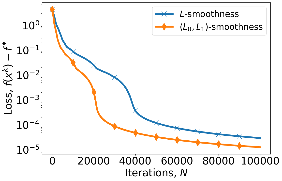
Figure 2: Comparison of SGD convergence behavior depending on the type of smoothness. Here we optimize $f$ with the parameters: $d=300$ (dimensional of problem), $B=1000$ (batch size).

02

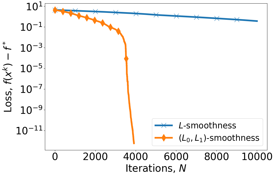
Figure 3: Comparison of NSGD convergence behavior depending on the type of smoothness. Here we optimize $f$ with the parameters: $d=300$ (dimensional of problem), $B=600$ (batch size), $\lambda=0.01$ (hyperparameter).

In Figure 3, we confirm our theoretical results for SGD (Algorithm 1), in particular Theorem 3.1. We see that there is an advantage in using generalized smoothness as claimed. However, a more significant advantage in convergence over iterations is observed for the Algorithm 2 (NSGD, see Figure 3). Indeed, we observe a significant improvement in iteration complexity, confirming our theoretical estimates (see Theorem 3.5).

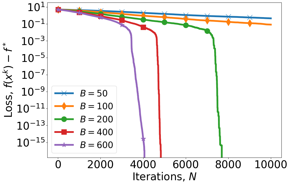
Figure 4: Comparison of NSGD convergence behavior depending on the batch size $B$. Here we optimize $f$ with the parameters: $d=300$ (dimensional of problem), $B=\{50,100,200,400,600\}$ (batch size), $\lambda=0.01$ (hyperparameter).

02

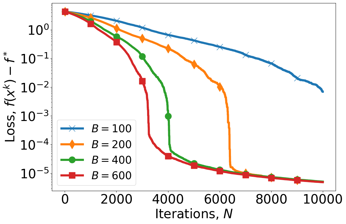
Figure 5: Comparison of ClipSGD convergence behavior depending on the batch size $B$. Here we optimize $f$ with the parameters: $d=300$ (dimensional of problem), $B=\{100,200,400,600\}$ (batch size), $c=0.01$ (clipping radius).

Analyzing the effect of the batch size we see on Figure 5 that increasing the batch size improves the iteration complexity $N$ of NSGD, which follows from the theoretical results. A similar dependence is observed for ClipSGD (Algorithm 3, see Figure 5). However, unlike NSGD, we see that CLipSGD improves the ’error floor’ convergence that follows due to switching to SGD regime $c>\left\|\mathbf{g}(x,\bm{\xi})\right\|$. To improve not only rate but also accuracy, it is necessary to decrease the size of the clipping radius $c$, as shown in Figure 1.

References

- Agarwal et al. (2010) Agarwal, A., Dekel, O., and Xiao, L. Optimal algorithms for online convex optimization with multi-point bandit feedback. In Colt, pp. 28–40. Citeseer, 2010.
- Akhavan et al. (2021) Akhavan, A., Pontil, M., and Tsybakov, A. Distributed zero-order optimization under adversarial noise. Advances in Neural Information Processing Systems, 34:10209–10220, 2021.
- Akhavan et al. (2022) Akhavan, A., Chzhen, E., Pontil, M., and Tsybakov, A. A gradient estimator via l1-randomization for online zero-order optimization with two point feedback. Advances in Neural Information Processing Systems, 35:7685–7696, 2022.
- Alistarh et al. (2018) Alistarh, D., Hoefler, T., Johansson, M., Konstantinov, N., Khirirat, S., and Renggli, C. The convergence of sparsified gradient methods. Advances in Neural Information Processing Systems, 31, 2018.
- Anonymous (2025) Anonymous, A. Maximum noise level as third optimality criterion in black-box optimization problem, 2025. URL https://openreview.net/forum?id=SWg72N2ky1.
- Bach & Perchet (2016) Bach, F. and Perchet, V. Highly-smooth zero-th order online optimization. In Conference on Learning Theory, pp. 257–283. PMLR, 2016.
- Bello et al. (2017) Bello, I., Zoph, B., Vasudevan, V., and Le, Q. V. Neural optimizer search with reinforcement learning. In International Conference on Machine Learning, pp. 459–468. PMLR, 2017.
- Bengio et al. (1994) Bengio, Y., Simard, P., and Frasconi, P. Learning long-term dependencies with gradient descent is difficult. IEEE transactions on neural networks, 5(2):157–166, 1994.
- Bogolubsky et al. (2016) Bogolubsky, L., Dvurechenskii, P., Gasnikov, A., Gusev, G., Nesterov, Y., Raigorodskii, A. M., Tikhonov, A., and Zhukovskii, M. Learning supervised pagerank with gradient-based and gradient-free optimization methods. Advances in neural information processing systems, 29, 2016.
- Bottou (1998) Bottou, L. Online algorithms and stochastic approximations. Online learning in neural networks, 1998.
- Bottou et al. (2018) Bottou, L., Curtis, F. E., and Nocedal, J. Optimization methods for large-scale machine learning. SIAM review, 60(2):223–311, 2018.
- Boyd (2004) Boyd, S. Convex optimization. Cambridge UP, 2004.
- Chen et al. (2023) Chen, Z., Zhou, Y., Liang, Y., and Lu, Z. Generalized-smooth nonconvex optimization is as efficient as smooth nonconvex optimization. In International Conference on Machine Learning, pp. 5396–5427. PMLR, 2023.
- Dean et al. (2012) Dean, J., Corrado, G., Monga, R., Chen, K., Devin, M., Mao, M., Ranzato, M., Senior, A., Tucker, P., Yang, K., et al. Large scale distributed deep networks. Advances in neural information processing systems, 25, 2012.
- Demidovich et al. (2023) Demidovich, Y., Malinovsky, G., Sokolov, I., and Richtárik, P. A guide through the zoo of biased sgd. Advances in Neural Information Processing Systems, 36:23158–23171, 2023.
- Dimlioglu & Choromanska (2024) Dimlioglu, T. and Choromanska, A. Grawa: Gradient-based weighted averaging for distributed training of deep learning models. In International Conference on Artificial Intelligence and Statistics, pp. 2251–2259. PMLR, 2024.
- Duchi et al. (2011) Duchi, J., Hazan, E., and Singer, Y. Adaptive subgradient methods for online learning and stochastic optimization. Journal of machine learning research, 12(7), 2011.
- Faw et al. (2023) Faw, M., Rout, L., Caramanis, C., and Shakkottai, S. Beyond uniform smoothness: A stopped analysis of adaptive sgd. In The Thirty Sixth Annual Conference on Learning Theory, pp. 89–160. PMLR, 2023.
- Gasnikov et al. (2022) Gasnikov, A., Novitskii, A., Novitskii, V., Abdukhakimov, F., Kamzolov, D., Beznosikov, A., Takac, M., Dvurechensky, P., and Gu, B. The power of first-order smooth optimization for black-box non-smooth problems. In International Conference on Machine Learning, pp. 7241–7265. PMLR, 2022.
- Gasnikov et al. (2023) Gasnikov, A., Dvinskikh, D., Dvurechensky, P., Gorbunov, E., Beznosikov, A., and Lobanov, A. Randomized gradient-free methods in convex optimization. In Encyclopedia of Optimization, pp. 1–15. Springer, 2023.
- Gasnikov et al. (2024) Gasnikov, A., Lobanov, A., and Stonyakin, F. Highly smooth zeroth-order methods for solving optimization problems under the pl condition. Computational Mathematics and Mathematical Physics, 64(4):739–770, 2024.
- Goodfellow (2016) Goodfellow, I. Deep learning, 2016.
- Gorbunov et al. (2020) Gorbunov, E., Danilova, M., and Gasnikov, A. Stochastic optimization with heavy-tailed noise via accelerated gradient clipping. Advances in Neural Information Processing Systems, 33:15042–15053, 2020.
- Gorbunov et al. (2024) Gorbunov, E., Tupitsa, N., Choudhury, S., Aliev, A., Richtárik, P., Horváth, S., and Takáč, M. Methods for convex -smooth optimization: Clipping, acceleration, and adaptivity. arXiv preprint arXiv:2409.14989, 2024.
- Hazan et al. (2015) Hazan, E., Levy, K., and Shalev-Shwartz, S. Beyond convexity: Stochastic quasi-convex optimization. Advances in neural information processing systems, 28, 2015.
- Hernández-Lobato et al. (2014) Hernández-Lobato, J. M., Hoffman, M. W., and Ghahramani, Z. Predictive entropy search for efficient global optimization of black-box functions. Advances in neural information processing systems, 27, 2014.
- Hübler et al. (2024a) Hübler, F., Fatkhullin, I., and He, N. From gradient clipping to normalization for heavy tailed sgd. arXiv preprint arXiv:2410.13849, 2024a.
- Hübler et al. (2024b) Hübler, F., Yang, J., Li, X., and He, N. Parameter-agnostic optimization under relaxed smoothness. In International Conference on Artificial Intelligence and Statistics, pp. 4861–4869. PMLR, 2024b.
- Juditsky & Nemirovski (2010) Juditsky, A. B. and Nemirovski, A. S. First order methods for nonsmooth convex large-scale optimization, i: General purpose methods. Optimization for Machine Learning, pp. 1–28, 2010.
- Kairouz et al. (2021) Kairouz, P., McMahan, H. B., Avent, B., Bellet, A., Bennis, M., Bhagoji, A. N., Bonawitz, K., Charles, Z., Cormode, G., Cummings, R., et al. Advances and open problems in federated learning. Foundations and trends® in machine learning, 14(1–2):1–210, 2021.
- Koloskova et al. (2023) Koloskova, A., Hendrikx, H., and Stich, S. U. Revisiting gradient clipping: Stochastic bias and tight convergence guarantees. In International Conference on Machine Learning, pp. 17343–17363. PMLR, 2023.
- Lacoste-Julien et al. (2012) Lacoste-Julien, S., Schmidt, M., and Bach, F. A simpler approach to obtaining an o (1/t) convergence rate for the projected stochastic subgradient method. arXiv preprint arXiv:1212.2002, 2012.
- Lan (2012) Lan, G. An optimal method for stochastic composite optimization. Mathematical Programming, 133(1):365–397, 2012.
- Lattimore & Gyorgy (2021) Lattimore, T. and Gyorgy, A. Improved regret for zeroth-order stochastic convex bandits. In Conference on Learning Theory, pp. 2938–2964. PMLR, 2021.
- Lee et al. (2024) Lee, H., Cho, H., Kim, H., Gwak, D., Kim, J., Choo, J., Yun, S.-Y., and Yun, C. Plastic: Improving input and label plasticity for sample efficient reinforcement learning. Advances in Neural Information Processing Systems, 36, 2024.
- Li et al. (2023) Li, H., Rakhlin, A., and Jadbabaie, A. Convergence of adam under relaxed assumptions. Advances in Neural Information Processing Systems, 36:52166–52196, 2023.
- Lobanov & Gasnikov (2023) Lobanov, A. and Gasnikov, A. Accelerated zero-order sgd method for solving the black box optimization problem under “overparametrization” condition. In International Conference on Optimization and Applications, pp. 72–83. Springer, 2023.
- Lobanov et al. (2024a) Lobanov, A., Bashirov, N., and Gasnikov, A. The “black-box” optimization problem: Zero-order accelerated stochastic method via kernel approximation. Journal of Optimization Theory and Applications, pp. 1–36, 2024a.
- Lobanov et al. (2024b) Lobanov, A., Gasnikov, A., Gorbunov, E., and Takác, M. Linear convergence rate in convex setup is possible! gradient descent method variants under -smoothness. arXiv preprint arXiv:2412.17050, 2024b.
- Nesterov (2013) Nesterov, Y. Introductory lectures on convex optimization: A basic course, volume 87. Springer Science & Business Media, 2013.
- Nesterov & Spokoiny (2017) Nesterov, Y. and Spokoiny, V. Random gradient-free minimization of convex functions. Foundations of Computational Mathematics, 17(2):527–566, 2017.
- Nguyen & Balasubramanian (2022) Nguyen, A. and Balasubramanian, K. Stochastic zeroth-order functional constrained optimization: Oracle complexity and applications. INFORMS Journal on Optimization, 2022.
- Pascanu et al. (2013) Pascanu, R., Mikolov, T., and Bengio, Y. On the difficulty of training recurrent neural networks. In Dasgupta, S. and McAllester, D. (eds.), Proceedings of the 30th International Conference on Machine Learning, volume 28 of Proceedings of Machine Learning Research, pp. 1310–1318, Atlanta, Georgia, USA, 17–19 Jun 2013. PMLR. URL https://proceedings.mlr.press/v28/pascanu13.html.
- Patel et al. (2022) Patel, K. K., Saha, A., Wang, L., and Srebro, N. Distributed online and bandit convex optimization. In OPT 2022: Optimization for Machine Learning (NeurIPS 2022 Workshop), 2022.
- Platt (1998) Platt, J. C. Fast training of support vector machines using sequential minimal optimization. Advances in Kernel Methods - Support Vector Learning, MIT Press, 1998.
- Polyak (1987) Polyak, B. T. Introduction to optimization. Optimization Software, Inc. Publications Division, New York, 1987.
- Shamir (2017) Shamir, O. An optimal algorithm for bandit and zero-order convex optimization with two-point feedback. The Journal of Machine Learning Research, 18(1):1703–1713, 2017.
- Stich & Karimireddy (2019) Stich, S. U. and Karimireddy, S. P. The error-feedback framework: Better rates for sgd with delayed gradients and compressed communication. arXiv preprint arXiv:1909.05350, 2019.
- Takezawa et al. (2024) Takezawa, Y., Bao, H., Sato, R., Niwa, K., and Yamada, M. Parameter-free clipped gradient descent meets polyak. In The Thirty-eighth Annual Conference on Neural Information Processing Systems, 2024.
- Vankov et al. (2024) Vankov, D., Rodomanov, A., Nedich, A., Sankar, L., and Stich, S. U. Optimizing -smooth functions by gradient methods. arXiv preprint arXiv:2410.10800, 2024.
- Vaswani et al. (2019) Vaswani, S., Bach, F., and Schmidt, M. Fast and faster convergence of sgd for over-parameterized models and an accelerated perceptron. In The 22nd international conference on artificial intelligence and statistics, pp. 1195–1204. PMLR, 2019.
- Wang et al. (2023) Wang, B., Zhang, H., Ma, Z., and Chen, W. Convergence of adagrad for non-convex objectives: Simple proofs and relaxed assumptions. In The Thirty Sixth Annual Conference on Learning Theory, pp. 161–190. PMLR, 2023.
- Woodworth et al. (2021) Woodworth, B. E., Bullins, B., Shamir, O., and Srebro, N. The min-max complexity of distributed stochastic convex optimization with intermittent communication. In Conference on Learning Theory, pp. 4386–4437. PMLR, 2021.
- Yuan & Ma (2020) Yuan, H. and Ma, T. Federated accelerated stochastic gradient descent. Advances in Neural Information Processing Systems, 33:5332–5344, 2020.
- Zhang et al. (2019) Zhang, J., He, T., Sra, S., and Jadbabaie, A. Why gradient clipping accelerates training: A theoretical justification for adaptivity. In International Conference on Learning Representations, 2019.
- Zhang et al. (2020) Zhang, J., Karimireddy, S. P., Veit, A., Kim, S., Reddi, S., Kumar, S., and Sra, S. Why are adaptive methods good for attention models? Advances in Neural Information Processing Systems, 33:15383–15393, 2020.
- Zhang et al. (2015) Zhang, S., Choromanska, A. E., and LeCun, Y. Deep learning with elastic averaging sgd. Advances in neural information processing systems, 28, 2015.
- Zhao et al. (2021) Zhao, S.-Y., Xie, Y.-P., and Li, W.-J. On the convergence and improvement of stochastic normalized gradient descent. Science China Information Sciences, 64:1–13, 2021.
- Zhao et al. (2024) Zhao, S.-Y., Shi, C.-W., Xie, Y.-P., and Li, W.-J. Stochastic normalized gradient descent with momentum for large-batch training. Science China Information Sciences, 67(11):212101, 2024.
- Zorich & Paniagua (2016) Zorich, V. A. and Paniagua, O. Mathematical analysis II, volume 220. Springer, 2016.
APPENDIX