Fits of $\alpha_{s}$ from event-shapes in the three-jet region: extension to all energies

Abstract

This work is an extension of a previous publication Nason:2023asn where we fitted the strong coupling $\alpha_{s}$ together with the non-perturbative parameter $\alpha_{0}$ from event-shape and jet-shape distributions using power corrections computed in the three-jet region. In ref. Nason:2023asn only ALEPH data at the $Z$-pole were used in the fit. Here, instead, we include a large data sample from various $e^{+}e^{-}$ experiments at energies ranging from 22 to 207 GeV and revisited the treatment of theoretical uncertainties. We find that the inclusion of different energies, while not changing the central fit result considerably, helps to disentangle the dependence of perturbative and non-perturbative corrections. Our best fit result is $\alpha_{s}(M_{Z})=0.1181\begin{subarray}{c}+0.0002\\ -0.0005\end{subarray}\begin{subarray}{c}+0.0018\\ -0.0021\end{subarray}$, where the first error includes experimental uncertianties and the second one includes uncertainties associated with scale variation, mass effects, fit limits, non-perturbative schemes and non-perturbative uncertainties.

1 Introduction

The determination of the strong coupling $\alpha_{s}$ from shape variables in the three-jet region in $e^{+}e^{-}$-annihilation has always been considered the simplest context where to perform such measurement, since the observables are dominated by terms of order $\alpha_{s}$. In spite of the long history of $e^{+}e^{-}$ QCD studies, this determination is controversial at present. On one side, these analyses show clearly the validity of QCD predictions. On the other, when requiring higher theoretical precision by including higher order in pertubation theory, different determinations do not seem consistent with each other, and some show a clear discrepancy with the world average (see e.g. the discussion in the 2024 Particle Data Group review on QCD ParticleDataGroup:2024cfk ).

Part of the problem is due to the fact that the most precise measurements of shape variables are carried out at the $Z$ peak, where the energy is not large enough for non-perturbative corrections to be negligible. In some analyses these effects are estimated using Monte Carlo models, while others use analytic approaches. One pitfall of the all analytic models used in the past is that they were obtained by extrapolating non-perturbative corrections calculated in the two-jet region to the regime of three-jets. This problem was addressed in refs. Luisoni:2020efy ; Caola:2021kzt ; Caola:2022vea and Nason:2023asn where ways were found to estimate the power corrections in the three-jet region. In particular, in ref. Nason:2023asn a fit of shape variables relying on the new calculation of power corrections was performed, leading to $\alpha_{s}$ values that were larger than those obtained using the previous method, and well compatible with the world average. Subsequent work on the subject Benitez:2024nav has to some extend addressed the issues raised in refs.Luisoni:2020efy ; Caola:2021kzt ; Caola:2022vea ; Nason:2023asn by restricting the fit-range to the two-jet region. Ref. Bell:2023dqs has instead addressed the question of whether theoretical uncertainties in the di-jet factorized predictions can have a sizeable impact on the $\alpha_{s}$ determination. The resummation of power-suppressed but logarithmically enhanced terms has recently been studies in ref. Dasgupta:2024znl .

A further concern, that was pointed out in ref. Nason:2023asn is the impact of resummed predictions in regions dominated by three well separated jets, where its validity is questionable. In spite of the fact that procedures to switch off resummation effects outside their region of validity are well established (e.g. through the use of modified logarithms or shape functions), it is often seen in practice that resummation effects lead to an increase of differential distributions by an amount which does not vanish even close ot the kinematic upper limit of the distributions, and instead amounts to a nearly constant factor larger than one. Given the availabity of more precise perturbative calculations, these resummed predictions can end up outside the fixed-order uncertainty band in the region where it should be most reliable. It is clear that larger theoretical predictions will typically lead to smaller values of the strong coupling, at times incompatible with the world average ParticleDataGroup:2024cfk .

A last issue, first pointed out in ref. Salam:2001bd , and which emerged in particular in the analyses of ref. Nason:2023asn , is the intrinsic ambiguity in shape variable definitions due to the finite values of hadron masses. In ref. Salam:2001bd three alternative schemes were proposed that lead to different results in shape variable distributions. Perturbative calculations deal with massless partons, and as such are not affected by such ambiguities, while the experimentally measured distributions are. It is however possible to use Monte Carlo generators to infer the shape variable distributions in these alternative schemes, starting from the distributions measured by the experiments in their standard scheme. This was found to be the largest source of uncertainties in ref. Nason:2023asn , suggesting that all determinations of the strong coupling from shape varibales should include this uncertainty. If one instead believes that non-perturbative hadron-mass effects can be absored into a re-parametrization of power-suppressed effects, one needs to verify that, when using these alternative schemes, all mass effects are absorbed into the non-perturbative function and that the $\alpha_{s}$ determimnations obtained are fully compatible. If this is not the case, a further uncertainty should be added.

The present work is a follow-up of ref. Nason:2023asn where we fitted the thrust, the $C$-parameter and the three-jet resolution variable $y_{3}$ in terms of the strong coupling constant $\alpha_{S}(M_{Z})$ and a non-perturbative parameter $\alpha_{0}$. The work of ref. Nason:2023asn was based upon two ingredients: the fixed-order calculation of shape-variable distributions at order $\alpha_{s}^{3}$ Gehrmann-DeRidder:2007foh ; Gehrmann-DeRidder:2007vsv ; Gehrmann-DeRidder:2008qsl ; DelDuca:2016csb , and a calculation of non-perturbative corrections based upon the findings of ref. Caola:2022vea . In ref. Nason:2023asn we used only ALEPH data taken on the $Z$ peak, while in the present work we use a much larger data-set with energies spanning from 22 to 207 GeV, available from different experiments, thus including a total of about 1400 data points.

A number of improvements have been implemented in our fit procedure. First, we now use a dynamical scale in the perturbative calculations, obtained by computing at leading order the average value of the transverse momentum of the perturbative gluon giving rise to the third jet for each value of the observable. A second improvement regards the inclusion, in the previous fits Nason:2023asn , of a theoretical error in the $\chi^{2}$ definition. This led to very small $\chi^{2}$ values, probably due to the fact that we did not include bin-by-bin theoretical error correlations. In this paper, we do not include a theoretical error in the $\chi^{2}$ definition, and obtain more reasonable values of $\chi^{2}$. The theoretical error is instead included as usual by performing suitable variations on the setup of the theory predictions. Third, we developed a procedure to determine the fit-range in an automated way which is valid for different observables and at different energies. Next, we developed an improved, adaptive procedure to find the minimum $\chi^{2}$ point in the ($\alpha_{s}$-$\alpha_{0}$)-plane that is fast enough also when using a large data set.

Since in the previous paper we considered a single energy, we found considerable degeneracy between the value of the strong coupling and the non-perturbative parameter, that was lifted in part by fitting simultaneously the three different observables. The inclusion of different energies lifts this degeneracy even further, allowing sensible fits also to single observables.

The paper is organised as follows. In Sec. 2 we present our theoretical framework and detail all changes compared to the previous setup. Sec. 2.2 recalls results and formulae for the non-perturbative corrections and discusses a few changes compared to ref. Nason:2023asn . In Sec. 3 we illustrate the dataset included in the fit. In Sec. 4 we explain our fit procedure. In Sec. 5 we present and discuss in detail our new fit result. In Sec. 5.4 we discuss the inclusion of the heavy-hemisphere mass and hemisphere mass difference in our fits. Our conclusions are presented in Sec. 6.

2 Theoretical framework and changes compared to previous methods

The variables of choice for our main fit are the thrust $T$ (or $\tau=1-T$), the $C$-parameter $C$, and three-jet resolution, $y_{23}$. As discussed in ref. Nason:2023asn we do not include in the main fit the heavy-jet mass $M_{H}^{2}$ and the jet-mass difference $M_{D}^{2}$, since for them the non-perturbative corrections have some undesirable features in the two-jet limit. We do however discuss them in Sec. 5.4, and perform a fit including them, showing that to some extent our calculation of power corrections describes them better than the previous (2-jet based) one.

All the variables that we consider in this work are defined in Sec. 2 of ref. Nason:2023asn , and we will not repeat the definition here. Similarly, ambiguities related to hadron masses are discussed in Sec. 3 of the same reference. Here we adopt the same default scheme choice (i.e. the $E$-scheme) and consider the $p$, $D$ and standard scheme as variations. As in the previous work, heavy-quark mass-effects are corrected for using Monte Carlos (see Sec. 6.2 of ref. Nason:2023asn ).

2.1 Calculation of the differential distributions

Our perturbative description of a shape-variable distribution $v$ relies on the perturbative computation of $e^{+}e^{-}\to 3$ jets at NNLO, performed using the public EERAD3 code Gehrmann-DeRidder:2007foh ; Gehrmann-DeRidder:2007vsv ; Gehrmann-DeRidder:2008qsl , which is based on the antenna subtraction formalism Gehrmann-DeRidder:2005btv .

The starting point is the cumulative distribution at center-of-mass energy $Q$ and renormalization scale $\mu_{R}$, which can be written as

$$\bar{\Sigma}_{\rm NNLO}(v,\mu_{R},Q)=\int_{v}^{1}dv^{\prime}\left[\frac{1}{\sigma_{\rm\scriptscriptstyle NNLO}}\frac{d\sigma_{\rm\scriptscriptstyle NNLO}(v^{\prime},\mu_{R},Q)}{dv^{\prime}}\right]_{\rm trunc}\,,$$ (1)

where the suffix “trunc” indicates that the ratio in the square bracket is expanded and truncated at NNLO order (see Eq.(5.2) of ref. Nason:2023asn ). We have

$$\bar{\Sigma}_{\rm NNLO}(v,\mu_{R},Q)+\Sigma_{\rm NNLO}(v,\mu_{R},Q)=1\,,$$ (2)

where $\Sigma_{\rm NNLO}(v,\mu_{R},Q)$ is given in Eq. (5.1) of ref. Nason:2023asn . Using $\bar{\Sigma}_{\rm NNLO}$ rather than $\Sigma_{\rm NNLO}$ (as was done in ref. Nason:2023asn ), avoids the need to specify how to handle the (divergent) $v\to 0$ region.

Here, at variance with ref. Nason:2023asn , we evaluate eq. (1) using a dynamical scale $\mu_{R}$, that is a function of the integration limit $v$. To obtain the contribution to a bin of the shape variable, we take the difference between $\bar{\Sigma}(v,\mu_{R}(v),Q)$ evaluated at the endpoints of the bin.

Our choice for the dynamical scale is the average transverse momentum for a given value of $v$ relative to the thrust axis computed at Born level. It is obtained by first histogramming the average transverse momentum as a function of $v$ computed at Born level. The result is then fitted with a simple parametrization of the form $\langle k_{t}\rangle=a\cdot v^{b}$. This average transverse momentum is taken to be our central scale choice $\mu_{0}$. As usual, we will consider variations by a factor two above and below this value.

The second ingredient for the computation of the distributions is the implementation of the non-perturbative corrections. We implemented a few modifications with respect to ref. Nason:2023asn . In particular we now separate variations associated with how the non-perturbative shift is implemented (schemes a, b, and c) and with the effect of estimated quadratic power corrections. We discuss these aspects in detail in the following section.

2.2 Non-perturbative corrections schemes and uncertainties

We compute the non-perturbative cross section to the cumulative distributions of a shape variable $v$ using formulae (4.29) through (4.32) of ref. Nason:2023asn , which make use of the function $h_{v}(\eta,\phi)$, defined in eq. (4.6) of the same reference.. In practice, in our calculation, rather than using the definition of $H_{\rm NP}$ given in Eq. (4.32) we use the value that can be inferred from Eq. (4.29) and (5.5), that is commonly adopted in dispersive models Akhoury:1995sp ; Dokshitzer:1995qm ; Dokshitzer:1997iz ; Dokshitzer:1998pt .

In order to estimate quadratic power suppressed effects we now define $h_{v}(\eta,\phi)$ in the following way:

$${h}_{v}(\eta,\phi)=\lim_{l_{\perp}\to 0}\tilde{h}_{v}\left(\eta,\phi,\frac{|l_{\perp}|}{Q}\right)\,,$$ (3)

with

$$\tilde{h}_{v}\left(\eta,\phi,\frac{|l_{\perp}|}{Q}\right)=\frac{Q}{|l_{\perp}|}\left[v(\{P\},l)-v(\{p\})\right].$$ (4)

Furthermore, we introduce the following functions

$$\tilde{\zeta}_{1}\left(v,\frac{|l_{\perp}|}{Q}\right)=\sum_{\rm dip}\frac{C_{\rm dip}}{C_{F}}\left(\frac{\mathrm{d}\sigma_{B}}{\mathrm{d}v}\right)^{-1}\int\mathrm{d}\sigma_{B}(\Phi_{B})\int\mathrm{d}\eta\frac{\mathrm{d}\phi}{2\pi}\frac{\theta\left(v(\{P\},l)-v\right)-\theta(v(\{p\})-v)}{|l_{\perp}|/Q},$$ (5)

and

$$\tilde{\zeta}_{2}\left(v,\frac{|l_{\perp}|}{Q}\right)=\sum_{\rm dip}\frac{C_{\rm dip}}{C_{F}}\left(\frac{\mathrm{d}\sigma_{B}}{\mathrm{d}v}\right)^{-1}\int\mathrm{d}\sigma_{B}(\Phi_{B})\,\delta\left(v(\{p\})-v\right)\int\mathrm{d}\eta\frac{\mathrm{d}\phi}{2\pi}\tilde{h}_{v}\left(\eta,\phi,\frac{|l_{\perp}|}{Q}\right)\,,$$ (6)

where the second one is obtained from the first one by Taylor expanding the first $\theta$-function in eq. (5). Both expressions are modifications of the $\zeta(v)$ function that differ from it by terms of order $|l_{\perp}|$, and thus have the expansion

$$\tilde{\zeta}_{1/2}\left(v,\frac{|l_{\perp}|}{Q}\right))=\zeta(v)\left[1+\frac{|l_{\perp}|}{Q}\cdot c_{1/2}\left(v,\frac{|l_{\perp}|}{Q}\right)\right]\,,$$ (7)

where $c_{1/2}$ have a well defined limit for $|l_{\perp}|\to 0$. We compute the functions $\tilde{\zeta}_{1/2}$ numerically, by setting up a generator for $q\bar{q}g$ production plus an extra radiation with a fixed transverse momentum $|l_{\perp}|$ in the radiating dipole rest frame, including all recoil effects, as described in Sec. 4.4 of ref. Nason:2023asn . We choose $|l_{\perp}|/{Q}=0.01$, which we assume to be small enough to be close to the $|l_{\perp}|\to 0$ limit. The functions $c_{1/2}$ are then extracted using eq. (7). We thus define

$$K_{1/2}(v)=C\cdot c_{1/2}(v)\cdot H_{\rm NP},$$ (8)

where $C$ is a coefficient of order 1 that we take equal to 1, and in our implementation of the non-perturbative correction we use as default the shift

$$\delta_{\rm NP}(v)=\zeta(v)\cdot H_{\rm NP}\cdot\left(1+K_{1}(v)\right).$$ (9)

The cumulative distribution including non-perturbative corrections is then given by

$$\Sigma^{\rm(a)}(v)=\Sigma_{\rm NNLO}(v-\delta_{\rm NP}(v)).$$ (10)

This defines our default scheme for the calculation of non-perturbative corrections, which we denote as (a). As alternatives we also propose schemes (b) and (c) defined as

$$\Sigma^{\rm(b)}(v) = \Sigma_{\rm LO}(v-\delta_{\rm NP}(v))+\Sigma_{\rm NNLO}(v)-\Sigma_{\rm LO}(v)\,,$$ (11)

$$\Sigma^{\rm(c)}(v) = \Sigma_{\rm NNLO}(v)-\delta_{\rm NP}(v)\frac{\mathrm{d}\Sigma_{\rm LO}(v)}{\mathrm{d}v}.$$ (12)

In ref. Nason:2023asn we also considered a scheme (d), that is as scheme (a) but without including the $K(v)$ term. In the present work instead we prefer to include explicitly separate variations associated with missing higher order power corrections in the $\zeta$ functions. We define for this purpose

$$\delta\Sigma_{\rm NP}(v)=|\Sigma^{\rm(a)}(v)-\Sigma_{\rm NNLO}(v)|\cdot\max(|K_{1}(v)|,|K_{2}(v)|).$$ (13)

The variations labeled npup (npdn) in the results presented in this paper are obtained by adding (subtracting) $\delta\Sigma_{\rm NP}(v)$ to the cumulants computed according to our default method (a).

2.3 Determination of fit ranges

We first compute the lower limit of the fit range as the peak position in the data multiplied by a factor $C_{ll}$, that we set by default equal to two. This choice guarantees that one is sufficiently far away from the region where resummation effects become important. The peak position is loosely fitted with a simple parametrization of the form $v_{\rm peak}(E)=v_{0}\cdot(91.2/E)^{a}$, where $v_{0}$ is the position of the peak at energy 91.2 GeV. In the case of $y_{3}$ we freeze the lower limit that at the $Z$-pole for energies above $M_{Z}$. The reason to do this is that at higher energies the peak position reaches very low $y_{3}$ values. Furthermore, we also determine a lower limit by imposing that the running renormalization scale never falls below 4 GeV. The final lower limit is taken equal to the maximum of the limits found with the two methods.

The upper limits of the fit-ranges are taken close to the kinematical bound for three parton production, and are set to 0.6 for the $C$-parameter and 0.3 for $\tau$ and $y_{3}$.

3 Description of data set used

To perform our fits, we used data collected at energies between 22 and 207 GeV from the ALEPH ALEPH:2003obs , DELPHI DELPHI:1999vbd ; DELPHI:2000uri ; DELPHI:2003yqh , JADE MovillaFernandez:1997fr , L3 L3:1992nwf ; L3:2002oql ; L3:2004cdh , OPAL OPAL:1992dnu ; OPAL:1993pnw ; OPAL:2004wof , SLD SLD:1994idb and TRISTAN TOPAZ:1993vyh experiments, as well as the combined analysis of $y_{3}$ using data from JADE and OPAL JADE:1999zar , which we refer to as JADE-OPAL. The available energies and the observables used, for each experiment, are listed in Table 1. We have omitted data on $y_{3}$ by JADE and OPAL, for energies that are already included in JADE-OPAL. With this set of data, available in the HEPData database Maguire:2017ypu , taking into account our fit range, we include up to 915 data points in the fit.

Obs.	Experiment	Energies in GeV
$C$	ALEPH ALEPH:2003obs	91.2 133 161 172 183 189 200 206
$C$	DELPHI DELPHI:1999vbd ; DELPHI:2000uri ; DELPHI:2003yqh	45 66 76 91.2 133 161 172 183 189 192 196 200 202 205 207
$C$	JADE MovillaFernandez:1997fr	35 44
$C$	L3 L3:1992nwf ; L3:2002oql ; L3:2004cdh	91.2 130.1 136.1 161.3 172.3 182.8 188.6 194.4 200
$C$	OPAL OPAL:1992dnu ; OPAL:1993pnw ; OPAL:2004wof	91.2 133 177 197
$C$	SLD SLD:1994idb	91.2
$T$	ALEPH ALEPH:2003obs	91.2 133 161 172 183 189 200 206
$T$	DELPHI DELPHI:1999vbd ; DELPHI:2000uri ; DELPHI:2003yqh	45 66 76 91.2 133 161 172 183 189 192 196 200 202 205 207
$T$	JADE MovillaFernandez:1997fr	35 44
$T$	L3 L3:1992nwf ; L3:2002oql ; L3:2004cdh	41.4 55.3 65.4 75.7 82.3 85.1 91.2 130.1 136.1 161.3 172.3
		182.8 188.6 194.4 200
$T$	OPAL OPAL:1992dnu ; OPAL:1993pnw ; OPAL:2004wof	91.2 133 177 197
$T$	SLD SLD:1994idb	91.2
$T$	TRISTAN TOPAZ:1993vyh	58
$y_{3}$	ALEPH ALEPH:2003obs	91.2 133 161 172 183 189 200 206
$y_{3}$	JADE MovillaFernandez:1997fr	22
$y_{3}$	JADE-OPAL JADE:1999zar	35 44 91.2 133 161 172 183 189
$y_{3}$	OPAL OPAL:1992dnu ; OPAL:1993pnw ; OPAL:2004wof	177 197
$y_{3}$	TRISTAN TOPAZ:1993vyh	58

Table 1: Summary of observables, experiments and energies used in the fit.

4 Fit procedure

We consider together all histogram bins of all shape variables from all experiments and at all energies that we include in the fit and label them with a single index. The $\chi^{2}$ is then defined as

$$\chi^{2}=\sum_{ij}\left(v_{i}-v_{i}^{(\rm th)}\right)V^{-1}_{ij}\left(v_{j}-v_{j}^{(\rm th)}\right),$$ (14)

where the covariance matrix is defined as

$$V_{ij}=\delta_{ij}R_{i}^{2}+(1-\delta_{ij})C_{ij}R_{i}R_{j}+{\rm Cov}^{(\rm Sys)}_{ij}\,,$$ (15)

where $R_{i}$ is the statistical error, $S_{i}$ the systematic error, $C_{ij}$ the statistical correlation matrix, and ${\rm Cov}^{(\rm Sys)}_{ij}$ the covariance matrix for the systematic errors. When systematic uncertainties are asymmetric we take the maximum of the two. For the calculation of the statistical and systematic covariance matrix we refer to ref. Nason:2023asn , Eq. (6.2) and (6.3), respectively.

In order to find the minimum $\chi^{2}$, as function of $\alpha_{s}$ and $\alpha_{0}$, we compute the $\chi^{2}$ on a rectangular grid of $\alpha_{s}$ and $\alpha_{0}$ points, and find the minimum value on the grid. The true minimum value of $\alpha_{s}$ ($\alpha_{0}$) is estimated using a quadratic interpolation of the three points on the grid: the grid minimum-point and its two neighboring points in the $\alpha_{s}$ ($\alpha_{0}$) direction. The $\chi^{2}$ value is taken as the average of the two interpolated values. While in ref. Nason:2023asn we could easily use grids with a large number of points to obtain an accurate result with this method, this is no longer feasible in the present case because of the very large number of data points. Therefore, we start the procedure with a grid with a modest number of points, find a minimum and iterate the procedure taking the minimum as the new center of the grid, reducing the grid range while keeping the same number of grid points. In practice, we typically start with a grid centered around $\alpha_{s}=0.12$ and $\alpha_{0}=0.5$, we use a grids which has 11 by 11 points, such that the maximum variation in $\alpha_{s}$ is $|\Delta\alpha_{s}|=0.01$ and $|\Delta\alpha_{0}|=0.5$. At each iteration we half the maximum variation. In general we perform four iterations. We have checked that performing more iterations the result remains stable. Once we have found the minimum, we compute $\chi^{2}$ values around the minimum on a relatively fine but sufficiently large grid, in order to compute the $\Delta\chi^{2}$ contours.

5 Results

We begin by presenting the simultaneous fit of the three shape variables $T$, $C$ and $y_{3}$, which we refer to as the CTy3 fit, using the full data set described in Sec. 3. We use our default central setup. The minimum $\chi^{2}$ and the contours for one and two units of $\chi^{2}$ above the minimum are shown in fig. 1.

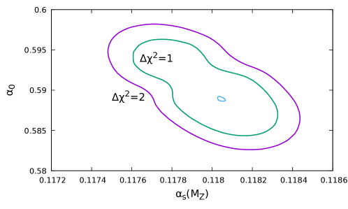
Figure 1: Fit central point and constant $\Delta\chi^{2}$ contours, for the simultaneous fit using $C$, $\tau$ and $y_{3}$.

This fit includes $N_{\rm deg}=895$ bins and has $\chi^{2}/N_{\rm deg}=1.26$. The central value of $\alpha_{s}$ is in good agreement with the world average and the value of the non-perturbative parameter agrees well with previous determinations (see e.g. Dasgupta:2003iq ).

The result of the fits performed using each observable separately and using the $C$-parameter and $\tau$ simultaneously are presented in Figs. 2,

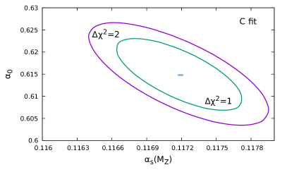
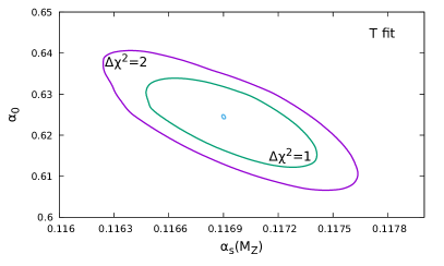
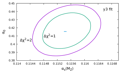
Figure 2: Fit central point and Constant $\Delta\chi^{2}$ contours for the fit of the $C$-parameter (left top) , $\tau$ (right top), y3 (left bottom) and CT (right bottom)

where C, T, y3 and CT label the $C$-parameter, $\tau$, $y_{3}$ and the simultaneous fits of $C$ and $\tau$, respectively. In fig. 3

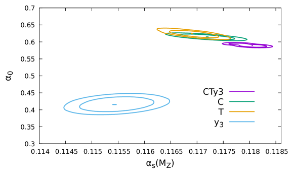
Figure 3: Fit central point and Constant $\Delta\chi^{2}$ contours for the CTy3, C, T and y3 fits reported on the same plot for comparison.

we report the CTy3, C, T and y3 fit on the same plot for comparison.

In table 2

Fit name	d.o.f.	$\chi^{2}$	$\chi^{2}/{\rm d.o.f.}$	$\alpha_{s}(M_{Z})$	$\alpha_{0}$
CTy3	895	1125.6	1.26	0.1181	0.5902
CT	744	952.6	1.28	0.1173	0.6089
C	292	269.0	0.921	0.1172	0.6148
T	452	651.7	1.44	0.1169	0.6245
y3	151	71.6	0.47	0.1155	0.4151

Table 2: Results for all fits.

we summarise the results of all fits. In table 3

Obs.	d.o.f.	$\chi^{2}$	$\chi^{2}/{\rm d.o.f.}$
$C$	292	278.2	0.95
$\tau$	452	659.7	1.465
$y_{3}$	151	132.7	0.879

Table 3: Individual $\chi^{2}$ contribution of each observable to the combined CTy3fit.

we present the $\chi^{2}$ and $\chi^{2}/{\rm d.o.f.}$ values computed for each separate observable at the $\alpha_{s}$ and $\alpha_{0}$ values determined with the CTy3 fit.

We observe that the $\chi^{2}/{\rm d.o.f.}$ value are quite acceptable for all fits. The T fit yields the largest $\chi^{2}/{\rm d.o.f.}$, and the y3 fit the smallest, both as individual fits and as contributions to the CTy3 fit. The individual fit to $y_{3}$ leads to a $\chi^{2}/{\rm d.o.f.}$ value that is very small (0.47), and to an $\alpha_{0}$ value that is not consistent with the other two determinations. However, due to the very low $\chi^{2}/{\rm d.o.f.}$ value, the $\chi^{2}$ for $y_{3}$ obtained using the $\alpha_{0}$ and $\alpha_{s}$ values of the CTy3 is still very reasonable.

Notice that the $\alpha_{s}(M_{Z})$ result of the CTy3 fit is larger than all individual determinations. This is not surprising if we look at the correlation between $\alpha_{s}(M_{Z})$ and $\alpha_{0}$ in fig. 2. In order to accommodate all observables with a single fit the value of $\alpha_{0}$ should be higher than the preferred $y_{3}$ value, and lower for the C and T fits, which implies larger values of $\alpha(M_{Z})$ in both cases.

5.1 Scale variations

Next, we consider the impact of performing a renormalizaton scale variation by factor 2 up and down in the theory predictions. The result is shown in Table 4.

Observable	scale	$\alpha_{s}(M_{Z})$	$\alpha_{0}$	$N_{\rm bins}$	$\chi^{2}/N_{\rm deg}$
	$\mu_{0}/2$	0.1167	0.67	816	2.38
CTy3	$\mu_{0}$	0.1181	0.59	895	1.26
	$2\mu_{0}$	0.1167	0.58	915	1.60
	$\mu_{0}/2$	0.1146	0.75	705	1.38
CT	$\mu_{0}$	0.1175	0.61	744	1.28
	$2\mu_{0}$	0.1211	0.50	744	1.34
	$\mu_{0}/2$	0.1141	0.76	285	0.99
C	$\mu_{0}$	0.1169	0.62	292	0.92
	$2\mu_{0}$	0.1212	0.51	292	0.95
	$\mu_{0}/2$	0.1159	0.71	420	1.52
T	$\mu_{0}$	0.1168	0.63	452	1.44
	$2\mu_{0}$	0.1208	0.53	452	1.52
	$\mu_{0}/2$	0.1122	0.03	111	0.53
y3	$\mu_{0}$	0.1155	0.42	151	0.47
	$2\mu_{0}$	0.1157	0.52	171	1.61

Table 4: Impact of scale variations on the results for all fits.

We see that in the CTy3 fit the value of $\alpha_{s}$ decreases slightly (by about 1.2%) both when varying the scale up or down. We find, however, larger values of $\chi^{2}$, especially when using a scale $\mu_{0}/2$. This result is better understood by examining the effect of scale variations in the individual C, T and y3 fits. In these cases we obtain much more reasonable $\chi^{2}$ values, although always worse than the central value. However the $\alpha(M_{Z})$ and $\alpha_{0}$ value obtained in the y3 fit for the scale choice $\mu_{0}/2$ is not compatible with that of the other determinations, which leads to the large $\chi^{2}/{\rm d.o.f.}$ value in the CTy3 fit. Some discrepancies of the fitted parameters in the C and T fits alone is also observed, but is not quite as strong, so that in the CT fit the increase in $\chi^{2}$ due to scale variations is not so large.

In conclusion, if we consider fits using individual variables, or the combined CT fit, we find large scale variations, of the order of 2-3%, while in the combined CTy3 fit the scale uncertainty amounts to about 1% on $\alpha_{s}s(M_{Z})$. This is in part due to the correlation between $\alpha_{s}(M_{Z})$ and $\alpha_{0}$. In fact, when the scale increases $\alpha_{s}(M_{Z})$ increases and $\alpha_{0}$ decreases for the C, T and CT fits, while for the y3 fit both $\alpha_{s}(M_{Z})$ and $\alpha_{0}$ increase.

5.2 Variations of other theory setting

When considering only scale variations, the extracted value of $\alpha_{s}(M_{Z})$ is confined in a range of 1.2%, suggesting that perhaps an extraction of $\alpha_{s}$ with a 0.6% accuracy may be possible. Unfortunately, by considering the other sources of uncertainties that were studied in ref. Nason:2023asn , this does not seem to be the case. All the considered uncertainties for the CTy3 fit are reported in table 5.

Variation	$\alpha_{s}(M_{Z})$	$\alpha_{0}$	$\chi^{2}$	$\chi^{2}/{\rm d.o.f.}$	d.o.f.
default	0.1181	0.5902	1125.6463	1.2577	895
$\mu_{R}=\mu_{0}/2$	0.1167	0.6683	1940.0007	2.3775	816
$\mu_{R}=2\mu_{0}$	0.1167	0.5846	1465.9393	1.6021	915
std scheme	0.1173	0.5347	1090.8732	1.2202	894
p scheme	0.1160	0.5624	1051.1005	1.1757	894
D scheme	0.1199	0.7252	747.3571	0.8350	895
$C_{\rm ll}=1.5$	0.1165	0.6260	1579.9496	1.6073	983
$C_{\rm ll}=3$	0.1177	0.5673	947.3134	1.2498	758
non-pert scheme (b)	0.1193	0.5923	1249.1436	1.3957	895
non-pert scheme (c)	0.1189	0.5825	1232.5919	1.3772	895
minus non-pert error	0.1187	0.5865	1122.1407	1.2538	895
plus non-pert error	0.1189	0.5649	1228.4413	1.3726	895

Table 5: Central fit result and variations of the results of the CTy3 fit, as described in the text. We indicate in boldface the central, highest and lowest values.

These include the scale variations, that we already discussed; the use of different mass schemes for the definition of the shape variables; variations on the lower limit of the fit range for each shape variable; three alternative different schemes for the calculation of the non-perturbative corrections; and the addition or subtraction of the non-perturbative error to the central value of the non-perturbative correction. In the following we describe them in turn.

5.2.1 Mass scheme dependence

It is easy to realise that there are alternative definitions of the same shape variable that yield the same results for massless final state particles, but not for massive ones. For example, in the definitions, the energy and the modulus of the momentum can be used interchangeably when dealing with massless particles, but this can makes a difference for massive ones. It thus turns out that for the family of schemes that agree in the massless case, the theoretical result is the same, while the measurements may differ Salam:2001bd . We stress that our calculation of the linear non-perturbative correction is also insensitive to mass effects, since at the end it always deals with massless particles in the final state, typically the particles that arise from the splitting of the soft gluon.

In ref. Salam:2001bd , besides the standard schemes commonly used by the experimental collaborations (reported in Sec. 2 of ref. Nason:2023asn ), three alternative schemes, dubbed E, p and D, where proposed. We assess the effect of the use of different schemes using a Monte Carlo generator, i.e. we generate a large sample of $e^{+}e^{-}\to{\rm hadrons}$ events using Pythia8  Sjostrand:2014zea , and for each measured distribution, we compute a migration matrix that can be used to convert from the standard scheme experimental data to the E, p or D scheme. More in detail for each generated event and for each measured binned event shape distribution, we compute the bin $i$ where the shape variable falls when using the standard scheme, and the bin $j$ where the shape variable falls when using the alternative scheme $S=$E, p or D. A corresponding migration matrix $T^{(S)}_{i,j}$ is then increased by one unit. At the end, the following equation holds

$$n_{j}^{(S)}=\sum_{i}n_{i}^{(\rm Std)}\frac{T^{(S)}_{i,j}}{\sum_{k}T^{(S)}_{ik}},$$ (16)

where $n_{i}^{(S)}$ is the number of events such that the observable computed in the scheme $S$ falls in bin $i$. We use the right hand side of eq. (16) using instead of the $n_{i}^{(\rm Std)}$ obtained with the Monte Carlo the one from data, so as to obtain the corrected data for the $S$ scheme.

By inspecting the table, we see that the effect of the mass scheme change yields the largest variation for the value of $\alpha_{s}$ both in the upper and lower directions. For this reason they are in boldface characters in the table. Furthermore, we find in all cases very reasonable values of $\chi^{2}$, so that we do not have a-posteriori reasons to exclude any scheme.

5.2.2 Fit range

The computation of the fit range is discussed in section 2.3, and is controlled by a parameter $C_{ll}$ that is set to two by default. We set $C_{ll}$ to 1.5 and 3 to assess the effect of lowering/rising the lower limit. We know that our calculation must fail for very low lower limits, due to the raising importance of Sudakov logarithms. We thus expect that the $\chi^{2}$ should become worse as we lower the lower limit, and be nearly constant as we raise it. This is in fact what we observe. By raising the limit the change in $\chi^{2}/{\rm d.o.f.}$ is very small, and the fitted values of $\alpha(M_{Z})$ and $\alpha_{0}$ change roughly by 0.3% and 4% respectively. On the other hand, when lowering the limit we get a variation in $\alpha(M_{Z})$ and $\alpha_{0}$ of 1.4% and 6% respectively, accompanied by a sharp increase in $\chi^{2}/{\rm d.o.f.}$, warning us not to venture further in that direction.

5.2.3 Implementation of the non-perturbative correction

A general summary of the calculation of non-perturbative correction is given in Sec. 2.2. Following the definitions given there, besides giving the value in our default scheme, we also present variations when using schemes (b) and (c).

5.2.4 Plus or minus the non-perturbative error

An estimate of missing corrections suppressed by more than one power of the non-perturbative scale, we follow the procedure illustrated in Sec. 2.2, that defines the npup and npdn variations.

5.2.5 General consideration on uncertainties

The variations reported in table 5 are of the order of 1%. The most prominent ones are those arising from changing the scheme for the treatment of light hadron masses, being equal to to +1.6-1.7%. Variation of the range lower limit leads also sizeable effect (1.3%). However, in this case we also observe a noticeable increase in $\chi^{2}$, which is not the case when varying the mass schemes.

The problem of ambiguities related to the hadron mass scheme is particularly severe. This is because they are sizeable, but also because the non-perturbative corrections due to light hadron masses cannot be studied in the large $n_{f}$ framework, since they always end up considering final states made up of massless partons. We remark that not many $\alpha_{s}$ fits in the context of $e^{+}e^{-}$ shape variables have considered the mass scheme ambiguities, while we find that they lead to dominant uncertainties.

On the other hand, we find that uncertainties related to how the non-perturbative corrections are included, and to possible higher-order non-perturbative corrections, are small, of the order of half a percent.

5.3 Comparison to previous parametrization of non-perturbative effects

Older studies of non-perturbative corrections were making use of the large $b_{0}$ approximate power corrections evaluate in the 2-jet region extrapolated to the full phase space. In our framework, this amounts to setting $\zeta(v)\to\zeta(0)$. We have performed such fits and report the result (including variations) in table 6.

Variation	$\alpha_{s}(M_{Z})$	$\alpha_{0}$	$\chi^{2}$	$\chi^{2}/{\rm d.o.f.}$	d.o.f.
default	0.1161	0.5389	1149.9394	1.2848	895
$\mu_{R}=\mu_{0}/2$	0.1155	0.6061	1523.6604	1.8672	816
$\mu_{R}=2\mu_{0}$	0.1150	0.5181	1830.6507	2.0007	915
std scheme	0.1153	0.4989	1106.6396	1.2379	894
p scheme	0.1141	0.5119	1125.7113	1.2592	894
D scheme	0.1173	0.6465	923.2022	1.0315	895
$C_{\rm ll}=1.5$	0.1143	0.5658	1510.5800	1.5367	983
$C_{\rm ll}=3$	0.1159	0.5325	977.2551	1.2893	758
non-pert scheme (b)	0.1163	0.5603	1281.1125	1.4314	895
non-pert scheme (c)	0.1167	0.5305	1312.8618	1.4669	895
minus non-pert error	0.1161	0.5390	1150.0007	1.2849	895
plus non-pert error	0.1161	0.5389	1149.8783	1.2848	895

Table 6: Results for the CTy3 fit using $\zeta(v)\to\zeta(0)$, and performing all variations that we have considered.

We find that in general the $\chi^{2}$ values that we obtain are as acceptable as for our standard fits. However, the value of $\alpha_{s}(M_{Z})$ that we obtained are systematically lower by two units in the third digit.

This trend holds also for the fits CT, and C, T, y3 as we can see in table 7.

	$\alpha_{s}(M_{Z})$
	CTy3		C		T		$y_{3}$
Variation	$\zeta(v)$	$\zeta(0)$	$\zeta(v)$	$\zeta(0)$	$\zeta(v)$	$\zeta(0)$	$\zeta(v)$	$\zeta(0)$
default	0.1181	0.1161	0.1169	0.1139	0.1168	0.1158	0.1155	0.1154
$\mu_{R}=\mu_{0}/2$	0.1167	0.1155	0.1141	0.1105	0.1159	0.1128	0.1122	0.1131
$\mu_{R}=2\mu_{0}$	0.1167	0.1150	0.1212	0.1184	0.1208	0.1191	0.1157	0.1161
std scheme	0.1173	0.1153	0.1164	0.1118	0.1152	0.1148	0.1150	0.1149
p scheme	0.1160	0.1141	0.1164	0.1118	0.1152	0.1148	0.1137	0.1135
D scheme	0.1199	0.1173	0.1190	0.1153	0.1205	0.1170	0.1168	0.1166
$C_{\rm ll}=1.5$	0.1165	0.1143	0.1151	0.1116	0.1154	0.1133	0.1142	0.1142
$C_{\rm ll}=3$	0.1177	0.1159	0.1221	0.1116	0.1180	0.1172	0.1156	0.1154
non-pert scheme (b)	0.1193	0.1163	0.1191	0.1176	0.1185	0.1184	0.1154	0.1154
non-pert scheme (c)	0.1189	0.1167	0.1195	0.1172	0.1192	0.1191	0.1154	0.1154
minus non-pert error	0.1187	0.1161	0.1173	0.1139	0.1165	0.1158	0.1157	0.1154
plus non-pert error	0.1189	0.1161	0.1172	0.1139	0.1172	0.1158	0.1153	0.1154

Table 7: Summary of $\alpha_{s}(M_{Z})$ results for all fits and variations considered.

5.4 Including the heavy-jet mass and the jet-mass difference in the fits

In ref. Nason:2023asn it was shown that the $\zeta$ functions for the heavy jet mass and for the jet mass difference undergo very sharp variations near the two jet limit configuration. We then preferred not to include them in our fit. Nevertheless, we were able to show that their behaviour in the three-jet region is in nice agreement with our calculation of non-perturbative corrections, that for these observables are in fact negative. It is thus interesting to see what happens if one attempts to include also these observables in the fits. In order to do this, we face an immediate problem, namely that the DELPHI data seem to be inconsistent with data from other experiments. Since the ALEPH experiment provides very precise data, which are in agreement with all other experiments, in the following, we show comparisons of DELPHI to ALEPH data at the $Z$-peak as an illustration. Since the two experiments use a very different binning, to illustrate the comparison, it is useful to take as a reference the theoretical prediction, which we show both including and omitting the non-perturbative correction. This comparison is displayed in Fig. 4 and 5 left and central panels.

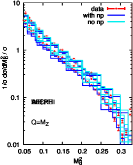
Figure 4: Comparison of ALEPH, DELPHI and WICKE data for $M_{h}^{2}$ distribution at $Q=M_{Z}$.

Figure 5: Same as Fig. 4 for the $M_{d}^{2}$ distribution.

It is clear that ALEPH data, which use a much finer binning than the DELPHI ones, are in excellent agreement with the theory prediction which includes the non-perturbative correction. Instead, the DELPHI data is considerably above both predictions. This is the case for both mass distributions. This is a clear indication that the experimental data are not consistent with each other. On the other hand, DELPHI data have been also re-analysed at $Q=M_{Z}$ in ref. Wicke:1999zz . These data, that we label “WICKE” in the following, are shown in the right panels of Figs. 4 and 5. We notice that these data are in good agreement with theory predictions including non-perturbative corrections, and therefore are compatible with ALEPH (and all other) data. For this reason, in the following, we have decided to omit in the fit all DELPHI data on $\rm M_{h}^{2}$ and $\rm M_{d}^{2}$ and to include instead data from ref. Wicke:1999zz , that we denote as “WICKE”.

In Table 8 we show all additional data that we have included in the fit. We use as upper limits for the fit ranges 0.33 in both cases, while the lower limits are set as described before. In Table 9 we show the results of our fit.

Obs.	Experiment	Energies in GeV
$M_{d}^{2}$	ALEPH ALEPH:2003obs	91.2 133 161 172 183 189 200 206
$M_{h}^{2}$	WICKE Wicke:1999zz	91.2
$M_{h}^{2}$	ALEPH ALEPH:2003obs	91.2 133 161 172 183 189 200 206
$M_{h}^{2}$	JADE MovillaFernandez:1997fr	35 44
$M_{h}^{2}$	L3 L3:1992nwf ; L3:2002oql ; L3:2004cdh	41.4 55.3 65.4 75.7 82.3 85.1 91.2 130.1 136.1 161.3 172.3
		182.8 188.6 194.4 200
$M_{h}^{2}$	OPAL OPAL:1992dnu ; OPAL:1993pnw ; OPAL:2004wof	91.2 133 177 197
$M_{h}^{2}$	SLD SLD:1994idb	91.2
$M_{h}^{2}$	TRISTAN TOPAZ:1993vyh	58
$M_{h}^{2}$	WICKE Wicke:1999zz	91.2

Table 8: Summary of data for $M_{h}^{2}$ and $M_{d}^{2}$ used in the section.

Variation	$\alpha_{s}(M_{Z})$	$\alpha_{0}$	$\chi^{2}$	$\chi^{2}/{\rm d.o.f.}$	d.o.f.
default	0.1214	0.5214	2737.0665	2.1267	1287
$\mu_{R}=\mu_{0}/2$	0.1200	0.5140	4602.1494	3.8968	1181
$\mu_{R}=2\mu_{0}$	0.1205	0.5380	4056.9046	3.1040	1307
std scheme	0.1221	0.4649	6032.3920	4.7055	1282
p scheme	0.1189	0.5007	2540.5896	1.9756	1286
D scheme	0.1253	0.6041	3605.6129	2.8016	1287
$C_{\rm ll}=1.5$	0.1224	0.5252	4238.7596	3.0191	1404
$C_{\rm ll}=3$	0.1199	0.5239	2076.6755	1.8692	1111
non-pert scheme (b)	0.1220	0.4810	4494.4234	3.4922	1287
non-pert scheme (c)	0.1221	0.4914	4148.3055	3.2232	1287
minus non-pert error	0.1216	0.5186	2769.4522	2.1519	1287
plus non-pert error	0.1212	0.5243	2710.8829	2.1064	1287

Table 9: As Table 5 but including also the data for $M_{h}^{2}$ and $M_{d}^{2}$ listed in Table 8.

We find that the inclusion of the masses in the fits increases the central value of $\alpha_{s}$ by about 2.8% and worsens in general all fits, yielding considerably larger $\chi^{2}$/d.o.f. values. Both features are mitigated when raising the lower limit of the fit range. This finding supports the view that perhaps the sharp variation of the $\zeta$ functions near the two-jet limit, found in ref. Nason:2023asn , introduces further uncertainty in the result near the two-jet region.

In Table 10 we show the same fit including mass-distributions, but now using the non-perturbative corrections computed in the two-jet limit. We find a reduction in the value of the fitted $\alpha_{s}(M_{Z})$, and considerably larger $\chi^{2}$ values, inidicating that constant non-perturbative corrections are incompatible with data.

Variation	$\alpha_{s}(M_{Z})$	$\alpha_{0}$	$\chi^{2}$	$\chi^{2}/{\rm d.o.f.}$	d.o.f.
default	0.1145	0.5769	6576.4898	5.1099	1287
$\mu_{R}=\mu_{0}/2$	0.1163	0.5983	3801.7747	3.2191	1181
$\mu_{R}=2\mu_{0}$	0.1068	0.6053	11697.8542	8.9502	1307
std scheme	0.1174	0.5225	5616.3416	4.3809	1282
p scheme	0.1110	0.5633	6437.6362	5.0059	1286
D scheme	0.1158	0.6806	10599.5174	8.2358	1287
$C_{\rm ll}=1.5$	0.1138	0.5865	6971.5191	4.9655	1404
$C_{\rm ll}=3$	0.1159	0.5735	5808.1213	5.2278	1111
non-pert scheme (b)	0.1170	0.5693	8415.0241	6.5385	1287
non-pert scheme (c)	0.1167	0.5491	8300.0328	6.4491	1287
minus non-pert error	0.1145	0.5770	6576.7989	5.1102	1287
plus non-pert error	0.1145	0.5769	6576.1813	5.1097	1287

Table 10: As Tables 9 but with power corrections computed in the two-jet limit.

We stress that, for the mass distributions, we have not included resummation effects in the two-jet limit, consistenly with what is done in the rest of the paper, nor all-order effects close to the symmetric three-particle limit ($M_{h}^{2}=M_{d}^{2}=1/3$), as studied in ref. Bhattacharya:2023qet . We find however that lowering the upper limit in our fit does not change the results in a noticeable way.

6 Conclusions

In this work, we have presented an extension of an analysis carried out in ref. Nason:2023asn , where we have fitted $e^{+}e^{-}$ shape-variable data using newly found results on power-corrections in the three-jet region Caola:2022vea . While in ref. Nason:2023asn only data collected at the $Z$ peak were considered, here we consider instead a large set of experiments and energies. We find results that are consistent with ref. Nason:2023asn , characterized by a value of $\alpha_{s}(M_{Z})$ well compatible with the world average but with sizeable uncertainties. Consistently with what observed in ref. Nason:2023asn also here we find that the dominant uncertainty is to due the ambiguity in the mass scheme.

A nice feature of this new analysis is that now, unlike in ref. Nason:2023asn , if we fit each variable individually, we also find reasonable determinations of the strong coupling, since the availability of different energies allows one to disentangle perturbative and non-perturbative effects. However, the associated errors for the individual fits are much larger than the one for the combined fit.

One feature of the newly found three-jet power corrections is that they are negative for the heavy-jet mass and jet-mass difference. Experimental data support this finding, as already remarked in ref. Nason:2023asn . Here we have shown that if we include the heavy-jet mass and jet-mass difference in the fits, in general we obtain large $\chi^{2}$ values, that are however much worse if we use as non-perturbative input the 2-jet determinations extrapolated to the three-jet region, as was done in earlier works.

In general, we stress that variations in the theory predictions lead to values of $\alpha_{s}$ that differ by up to three percent. This suggests that, once all relevant uncertainties are taken into account, a fit of $\alpha_{s}$ with an uncertainty below a percent seems out of reach.

We emphasize that our implementation of non-perturbative effects is the minimal and most straighforward one to verify the impact of non-perturbative corrections away from the two-jet limit. A further development of our work could be the inclusion of resummmation effects, together with a better treatment of the interplay between soft radiation and non-perturbative corrections.

References

- (1) P. Nason and G. Zanderighi, Fits of s using power corrections in the three-jet region, JHEP 06 (2023) 058, [arXiv:2301.03607].
- (2) Particle Data Group Collaboration, S. Navas et al., Review of particle physics, Phys. Rev. D 110 (2024), no. 3 030001.
- (3) G. Luisoni, P. F. Monni, and G. P. Salam, -parameter hadronisation in the symmetric 3-jet limit and impact on fits, Eur. Phys. J. C 81 (2021), no. 2 158, [arXiv:2012.00622].
- (4) F. Caola, S. Ferrario Ravasio, G. Limatola, K. Melnikov, and P. Nason, On linear power corrections in certain collider observables, JHEP 01 (2022) 093, [arXiv:2108.08897].
- (5) F. Caola, S. Ferrario Ravasio, G. Limatola, K. Melnikov, P. Nason, and M. A. Ozcelik, Linear power corrections to shape variables in the three-jet region, arXiv:2204.02247.
- (6) M. A. Benitez, A. H. Hoang, V. Mateu, I. W. Stewart, and G. Vita, On Determining from Dijets in Thrust, arXiv:2412.15164.
- (7) G. Bell, C. Lee, Y. Makris, J. Talbert, and B. Yan, Effects of renormalon scheme and perturbative scale choices on determinations of the strong coupling from e+e- event shapes, Phys. Rev. D 109 (2024), no. 9 094008, [arXiv:2311.03990].
- (8) M. Dasgupta and F. Hounat, Exploring soft anomalous dimensions for power corrections, arXiv:2411.16867.
- (9) G. P. Salam and D. Wicke, Hadron masses and power corrections to event shapes, JHEP 05 (2001) 061, [hep-ph/0102343].
- (10) A. Gehrmann-De Ridder, T. Gehrmann, E. W. N. Glover, and G. Heinrich, Infrared structure of e+ e- — 3 jets at NNLO, JHEP 11 (2007) 058, [arXiv:0710.0346].
- (11) A. Gehrmann-De Ridder, T. Gehrmann, E. W. N. Glover, and G. Heinrich, NNLO corrections to event shapes in e+ e- annihilation, JHEP 12 (2007) 094, [arXiv:0711.4711].
- (12) A. Gehrmann-De Ridder, T. Gehrmann, E. W. N. Glover, and G. Heinrich, Jet rates in electron-positron annihilation at O(alpha(s)**3) in QCD, Phys. Rev. Lett. 100 (2008) 172001, [arXiv:0802.0813].
- (13) V. Del Duca, C. Duhr, A. Kardos, G. Somogyi, and Z. Trócsányi, Three-Jet Production in Electron-Positron Collisions at Next-to-Next-to-Leading Order Accuracy, Phys. Rev. Lett. 117 (2016), no. 15 152004, [arXiv:1603.08927].
- (14) A. Gehrmann-De Ridder, T. Gehrmann, and E. W. N. Glover, Antenna subtraction at NNLO, JHEP 09 (2005) 056, [hep-ph/0505111].
- (15) R. Akhoury and V. I. Zakharov, On the universality of the leading, 1/Q power corrections in QCD, Phys. Lett. B 357 (1995) 646–652, [hep-ph/9504248].
- (16) Y. L. Dokshitzer, G. Marchesini, and B. R. Webber, Dispersive approach to power behaved contributions in QCD hard processes, Nucl. Phys. B 469 (1996) 93–142, [hep-ph/9512336].
- (17) Y. L. Dokshitzer, A. Lucenti, G. Marchesini, and G. P. Salam, Universality of 1/Q corrections to jet-shape observables rescued, Nucl. Phys. B 511 (1998) 396–418, [hep-ph/9707532]. [Erratum: Nucl.Phys.B 593, 729–730 (2001)].
- (18) Y. L. Dokshitzer, A. Lucenti, G. Marchesini, and G. P. Salam, On the universality of the Milan factor for 1 / Q power corrections to jet shapes, JHEP 05 (1998) 003, [hep-ph/9802381].
- (19) ALEPH Collaboration, A. Heister et al., Studies of QCD at e+ e- centre-of-mass energies between 91-GeV and 209-GeV, Eur. Phys. J. C 35 (2004) 457–486.
- (20) DELPHI Collaboration, P. Abreu et al., Energy dependence of event shapes and of alpha(s) at LEP-2, Phys. Lett. B 456 (1999) 322–340.
- (21) DELPHI Collaboration, P. Abreu et al., Consistent measurements of alpha(s) from precise oriented event shape distributions, Eur. Phys. J. C 14 (2000) 557–584, [hep-ex/0002026].
- (22) DELPHI Collaboration, J. Abdallah et al., A Study of the energy evolution of event shape distributions and their means with the DELPHI detector at LEP, Eur. Phys. J. C 29 (2003) 285–312, [hep-ex/0307048].
- (23) JADE Collaboration, P. A. Movilla Fernandez, O. Biebel, S. Bethke, S. Kluth, and P. Pfeifenschneider, A Study of event shapes and determinations of alpha-s using data of e+ e- annihilations at s**(1/2) = 22-GeV to 44-GeV, Eur. Phys. J. C 1 (1998) 461–478, [hep-ex/9708034].
- (24) L3 Collaboration, B. Adeva et al., Studies of hadronic event structure and comparisons with QCD models at the Z0 resonance, Z. Phys. C 55 (1992) 39–62.
- (25) L3 Collaboration, P. Achard et al., Determination of from hadronic event shapes in annihilation at 192-GeV = = 208-GeV, Phys. Lett. B 536 (2002) 217–228, [hep-ex/0206052].
- (26) L3 Collaboration, P. Achard et al., Studies of hadronic event structure in annihilation from 30-GeV to 209-GeV with the L3 detector, Phys. Rept. 399 (2004) 71–174, [hep-ex/0406049].
- (27) OPAL Collaboration, P. D. Acton et al., A Global determination of (M(z0) ) at LEP, Z. Phys. C 55 (1992) 1–24.
- (28) OPAL Collaboration, P. D. Acton et al., A Determination of alpha-s (M (Z0)) at LEP using resummed QCD calculations, Z. Phys. C 59 (1993) 1–20.
- (29) OPAL Collaboration, G. Abbiendi et al., Measurement of event shape distributions and moments in e+ e- — hadrons at 91-GeV - 209-GeV and a determination of alpha(s), Eur. Phys. J. C 40 (2005) 287–316, [hep-ex/0503051].
- (30) SLD Collaboration, K. Abe et al., Measurement of alpha-s (M(Z)**2) from hadronic event observables at the Z0 resonance, Phys. Rev. D 51 (1995) 962–984, [hep-ex/9501003].
- (31) TOPAZ Collaboration, Y. Ohnishi et al., Measurements of alpha-s in e+ e- annihilation at TRISTAN, Phys. Lett. B 313 (1993) 475–482.
- (32) JADE, OPAL Collaboration, P. Pfeifenschneider et al., QCD analyses and determinations of alpha(s) in e+ e- annihilation at energies between 35-GeV and 189-GeV, Eur. Phys. J. C 17 (2000) 19–51, [hep-ex/0001055].
- (33) E. Maguire, L. Heinrich, and G. Watt, HEPData: a repository for high energy physics data, J. Phys. Conf. Ser. 898 (2017), no. 10 102006, [arXiv:1704.05473].
- (34) M. Dasgupta and G. P. Salam, Event shapes in e+ e- annihilation and deep inelastic scattering, J. Phys. G 30 (2004) R143, [hep-ph/0312283].
- (35) T. Sjöstrand, S. Ask, J. R. Christiansen, R. Corke, N. Desai, P. Ilten, S. Mrenna, S. Prestel, C. O. Rasmussen, and P. Z. Skands, An introduction to PYTHIA 8.2, Comput. Phys. Commun. 191 (2015) 159–177, [arXiv:1410.3012].
- (36) D. Wicke, Energieabhängigkeit von Ereignisformobservablen und der starken Kopplung. PhD thesis, Wuppertal U., 1999.
- (37) A. Bhattacharya, J. K. L. Michel, M. D. Schwartz, I. W. Stewart, and X. Zhang, NNLL resummation of Sudakov shoulder logarithms in the heavy jet mass distribution, JHEP 11 (2023) 080, [arXiv:2306.08033].