Spacetime profile of electromagnetic fields in intermediate-energy heavy-ion collisions

Abstract

We numerically estimate the spacetime profile of the electromagnetic fields produced in intermediate-energy heavy-ion collisions $\sqrt{s_{{}_{\;\!\!N\;\!\!\;\!\!N}}}=2.4\,\mathchar 45\relax\,7.7\;{\rm GeV}$ for a wide range of impact parameters $b=0\,\mathchar 45\relax\,9\;{\rm fm}$, using a hadronic cascade model JAM (Jet AA Microscopic transport model). We demonstrate that (1) the produced electromagnetic fields are as strong as $eE,eB={\mathcal{O}}((50\;{\rm MeV})^{2})$; (2) that the produced fields extend in spacetime about $V_{4}={\mathcal{O}}((10\;{\rm fm})^{4})$; (3) that the magnetic field dominates around the collision point, while the other broad regions of spacetime are dominated by the electric field; and (4) that a topological electromagnetic-field configuration such that ${\bm{E}}\cdot{\bm{B}}\neq 0$ is realized.

I Introduction

The possibility of generating strong electromagnetic field in heavy-ion collisions has been discussed intensively over the past decade for the RHIC and LHC energy scale, where the collision energy $\sqrt{s_{{}_{\;\!\!N\;\!\!\;\!\!N}}}$ (i.e., the center-of-mass energy per a nucleon pair) is $\sqrt{s_{{}_{\;\!\!N\;\!\!\;\!\!N}}}={\mathcal{O}}(100\,\mathchar 45\relax\,5000\;{\rm GeV})$ [1]. Various transport-model simulations have been carried out, and it has been established that a very strong magnetic field is created in non-central collisions due to the Ampère law [2, 3, 4]. The magnitude of the magnetic field can reach $eB={\mathcal{O}}((0.1\,\mathchar 45\relax\,1\;{\rm GeV})^{2})$, which is the strongest field known in the present Universe, but it is at the same time extremely short-lived with lifetime of the order of ${\mathcal{O}}(0.01\,\mathchar 45\relax\,0.1\;{\rm fm}/c)$ (although there are discussions that the lifetime can be made longer by including finite electric conductivity [5, 6, 7, 8, 9, 10]). The generation of such a strong magnetic field has attracted a great deal of attention, in connection to, e.g., the chiral magnetic effect [11, 12], the phase diagram of quantum chromodynamics (QCD) in magnetic field [13, 14, 15], and non-linear quantum electrodynamics (QED) [16, 17]. The strong magnetic field can also leave intriguing experimental signatures. Such signatures have been observed in actual experiments recently, e.g., the first observations of the light-by-light scattering [18] and the linear Breit-Wheeler process [19, 20] and the charged directed flow [7, 21, 22, 23].

The past study of the strong electromagnetic field in heavy-ion collisions was motivated by the high-energy experiments, i.e., RHIC and the LHC. It is, however, one of the research trends of heavy-ion physics to lower the energy scale to investigate the intermediate energy regime such that $\sqrt{s_{{}_{\;\!\!N\;\!\!\;\!\!N}}}={\mathcal{O}}(2\,\mathchar 45\relax\,10\;{\rm GeV})$. Compared to the high-energy regime, which is suitable for creating a hot baryon-less matter, such an intermediate-energy regime is advantageous for creating a dense baryonic matter [24]. To explorer such a dense baryonic matter, or dense QCD physics broadly speaking, various experimental programs of intermediate-energy heavy-ion collisions are now being conducted (e.g., the Beam-Energy Scan (BES) program at RHIC [25] and NA61/SHINE at SPS [26]) and will be done worldwide (e.g., NICA [27], FAIR [28], HIAF [29], and J-PARC-HI [30]) [31].

Given the increasing interest to intermediate-energy heavy-ion collisions, it is natural to ask what the electromagnetic-field profile looks like in this energy regime. Compared to high-energ collisions, relatively few studies have explored this topic [32, 33, 34, 35, 36, 37]. Indeed, physical processes are much more involved due to the baryon stopping, while the system is almost transparent in the high-energy limit, meaning that intermediate-energy heavy-ion collisions require a more sophisticated microscopic treatment of heavy-ion reactions.

Understanding the electromagnetic-field profile is interesting not only because it has potential to induce novel QED/QCD/hadronic processes due to the field but also because it can contaminate signals of dense QCD physics. In fact, electromagnetic observables such as dileptons and photons can in principle be clean probes of the dense QCD physics, since they are transparent to the strong interaction. It is, thus, natural to look for such electromagnetic signatures of the dense QCD physics such as the color superconductor phase transition or the conjectured QCD critical point [38, 39, 40, 41]. However, these electromagnetic observables are expected to be modified by the presence of strong electromagnetic field and hence would blur the signals of the dense QCD physics (cf. the impact of the electromagetic field for the extraction of the symmetry energy [34]).

In addition to the motivation in heavy-ion physics, understanding of the strong electromagnetic field in intermediate-energy heavy-ion collisions is also of interest to the area of strong-field QED. In strong-field QED, there is an experimental difficulty that strong electromagnetic field beyond the critical field strength $eE_{\rm cr}:=m_{e}\approx(0.5\;{\rm MeV})^{2}$, where $e>0$ is the elementary charge and $m_{e}$ is the electron mass, cannot be achieved in laboratory experiments. The current strongest electromagnetic field is realized with intense laser, whose focused intensity is $I=1\times 10^{23}\;{\rm W/cm^{2}}$, corresponding to $E\approx 10^{-3}\,E_{\rm cr}$ [42]. The laser intensity is growing rapidly and continuously. Hence, the current intensity is envisaged to be surpassed by the latest and future facilities such as Extreme Light Infrastructure (ELI) $I={\mathcal{O}}(10^{25}\;{\rm W/cm^{2}})$ [43], which however is still far below the critical field strength $E_{\rm cr}$. Therefore, a novel method to create a strong electromagnetic field, other than intense laser, is highly appreciated. The strong electromagnetic field in intermediate-energy heavy-ion collisions can be a natural candidate to this.

The purpose of this paper is to investigate the spacetime profile of the electromagnetic field produced in intermediate-energy heavy-ion collisions with finite impact parameter. This work is an extension of the author’s previous paper [35], which focused on central collisions. By introducing finite impact parameter, we have an interplay between the electric and magnetic fields, which is what we want to understand in the present paper. Namely, in central collisions, the produced field is dominated by the Coulomb field emanating from the collisions remnants, and thus is purely electric. By increasing the impact parameter, we have additional electric current flowing circularly on the reaction plane, which in turn produces a magnetic field in the perpendicular direction with respect to the reaction plane via the Ampère law. Thus, the electric and magnetic fields coexist in non-central collisions, and how they coexist and evolve heavily depends on the dynamics, investigation of which requires a realistic transport-model simulation.

This paper is organized as follow: In Sec. II, we explain the numerical strategy adopted in this work. In Sec. III, we present our numerical results and discuss their physical meanings. Sec. IV is devoted to summary and discussion. We have one Appendix A, where additional plots are presented.

Notation.— Our beam axis is taken along the $z$-direction. We adopt the natural unit $\hbar=c=1$.

II Numerical scheme

We estimate the spacetime profile of the electromagnetic field in intermediate-energy heavy-ion collisions at finite impact parameter by using the numerical procedure performed in Ref. [35]. In this section, we briefly review this procedure.

We use an event generator, JAM, to calculate the electric current from the phase-space distributions of charged particles produced in collisions. JAM is a hadronic cascade model [44, 45] and has a feature that it includes resonances, string excitation, and mini-jet as basic inelastic particle production mechanisms to cover the broad collision energy range from a few GeV to more than one hundred GeV (see Ref. [46] for more on various model comparisons). We ran JAM with the default setting (i.e., no mean field nor hydro phase, which can be included as advanced options) in order to present a baseline result before taking into account such non-trivial physical effects.

From the spacetime positions obtained by JAM, we can calculate the electric current $J^{\mu}$ at position $(t,{\bm{x}})$ in a single event as

$$J(t,{\bm{x}})=\sum_{i\in{\rm all\ charged\ hadrons}}\frac{p^{\mu}_{i}}{p^{0}_{i}}q_{i}f(t,{\bm{x}})\;,$$ (1)

where $p^{\mu}_{i}$ and $q_{i}$ are the four-momentum and charge of $i$-th charged hadron at time $t$, respectively, and $f$ is a smearing function to convert the charge $q_{i}$ to the charge density $q_{i}f$. We adopt the relativistic Gaussian smearing function,

$$f(t,{\bm{x}}):=\frac{\gamma_{i}}{(\sqrt{2\pi}\sigma)^{3}}{\rm e}^{-\frac{|{\bm{x}}-{\bm{x}}_{i}|^{2}+\gamma_{i}^{2}\left({\bm{v}}_{i}\cdot({\bm{x}}-{\bm{x}}_{i})\right)^{2}}{2\sigma^{2}}}\;,$$ (2)

where ${\bm{x}}_{i},{\bm{v}}_{i}$, and $\gamma_{i}:=1/\sqrt{1-({\bm{v}}_{i})^{2}}$ are the position, velocity, and the gamma factor of the $i$-th charged hadron, respectively, and $\sigma$ is the smearing width, which we fix as 1 fm.

Once the electric current (1) is obtained, can we calculate the electromagnetic field from the retarded potential,

$$A^{\mu}(t,{\bm{x}}):=\frac{1}{4\pi}\int{\rm d}^{3}{\bm{x}}^{\prime}\frac{J^{\mu}(t-|{\bm{x}}-{\bm{x}}^{\prime}|,{\bm{x}}^{\prime})}{|{\bm{x}}-{\bm{x}}^{\prime}|}\;,$$ (3)

as

$${\bm{E}}_{n}:=-\partial_{t}{\bm{A}}-{\bm{\nabla}}A^{0}\ \ {\rm and}\ \ {\bm{B}}_{n}:={\bm{\nabla}}\times{\bm{A}}\;,$$ (4)

where we have added the subscript $n$ to emphasize that it is a single-event result at the $n$-th event. We carry out the integration in Eq. (3) numerically via the Gauss-Legendre quadrature method and the differentiation in Eq. (4) via the center differentiation, and confirmed that both are converging well with the numerical parameters used in the simulation.

In this paper, we are interested in an event-averaged value, rather than a single-event value obtained in Eq. (4). Therefore, we take the event averaging of the electromagnetic fields as

$${\bm{E}}:=\frac{1}{N}\sum_{n=1}^{N}{\bm{E}}_{n}\ \ {\rm and}\ \ {\bm{B}}:=\frac{1}{N}\sum_{n=1}^{N}{\bm{B}}_{n}\;,$$ (5)

where $N$ is the total number of events. Due to computational constraints, we chose a relatively small event number $N=100$. While this number is not large enough to completely eliminate event-by-event fluctuations, we have verified that it is sufficient for achieving a well-smoothed electromagnetic-field distribution in spacetime (see Sec. III) and for that the sensitivity to the choice of the smearing width $\sigma$ becomes negligible after the event averaging.

III Numerical results

We present the numerical results obtained by the program outlined in Sec. II and discuss the electromagnetic field generated in non-central collisions of gold ions at intermediate energies. Our main findings in this section are (1) that the produced electromagnetic fields are as strong as $eE,eB={\mathcal{O}}((50\;{\rm MeV})^{2})$; (2) that the produced fields extend in spacetime about $V_{4}={\mathcal{O}}((10\;{\rm fm})^{4})$; (3) that the magnetic field dominates only around the collision point, while the other broad regions of spacetime are dominated by the electric field; and (4) that a topological electromagnetic-field configuration such that ${\bm{E}}\cdot{\bm{B}}\neq 0$ is realized.

III.1 Spacetime profile

To develop a basic understanding of the electromagnetic field generated in intermediate-energy non-central heavy-ion collisions, we first discuss the spacetime profile of the produced field qualitatively by presenting some density plots. For demonstration purpose, the collision energy and impact parameter are fixed here as $\sqrt{s_{{}_{\;\!\!N\;\!\!\;\!\!N}}}=4.5\;{\rm GeV}$ and $b=6\;{\rm fm}$, but the qualitative features remain the same in other collision energies and impact parameters.

Fig. LABEL:fig:1 shows the spacetime evolution of an electromagnetic Lorentz invariant,

$${\mathcal{F}}:={\bm{E}}^{2}-{\bm{B}}^{2}\;.$$ (6)

See Appendix A for the same plots for each electromagnetic component $E_{x},E_{y},E_{z},B_{x},B_{y},$ and $B_{z}$.

Before observing the figure, we notice that the sign of the invariant ${\mathcal{F}}$ is important. It indicates whether the electric or magnetic component of the electromagnetic field at a spacetime point dominates, i.e., ${\mathcal{F}}>0$ means the field is electric, while ${\mathcal{F}}<0$ then magnetic. In the figure, ${\mathcal{F}}>0$ and ${\mathcal{F}}<0$ are represented by red and blue colors, respectively.

Observing Fig. LABEL:fig:1, we understand that the red region occupies the majority of the spacetime, while the blue region is confined to a small area near the center. This indicates that the produced electromagnetic fields are primarily dominated by the electric component throughout most of the spacetime, with the magnetic component becoming significant only in the central region. The majority of the electric field is simply the consequence of the long-range nature of the Coulomb law.

We also observe that the produced electromagnetic field is highly anisotropic: the spatial distribution is strongly squeezed in the beam $z$-direction. This is a direct consequence of the relativistic Lorentz contraction. It is notable that such a relativistic effect cannot be dismissed even at the intermediate-energy regime.

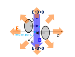
Figure 2: A schematic picture of how nonzero ${\mathcal{G}}$ emerges.

Next, we turn to consider another electromangetic Lorentz invariant,

$${\mathcal{G}}:={\bm{E}}\cdot{\bm{B}}\;,$$ (7)

which is shown in Fig. LABEL:fig:3

It is an interesting feature that ${\mathcal{G}}$ can be non-vanishing at intermediate-energy non-central heavy-ion collisions. An intuitive explanation of how ${\mathcal{G}}$ emerges is provided in Fig. 2. There are two physical processes contributing to the emergence of ${\mathcal{G}}$. First, the Coulomb electric field is generated by the charged matter formed by the collision participants. The resulting electric field emanates (roughly) radially from the collision point. Second, the magnetic field is produced according to Ampère’s law. The charged matter is not static but “rotates” due to the net angular momentum supplied by the finite impact parameter [47]. As a result, a circulating electric current exists around the $y$-axis, producing a magnetic field along the $-y$ direction. The resulting field directions are shown in Fig. 2. Clearly, the electric and magnetic fields are not orthogonal to each other, and hence ${\mathcal{G}}\neq 0$ is concluded. As a side note, it is also evident from the figure that (i) the magnitude of ${\mathcal{G}}$ becomes the largest (vanishes) on the $y$-axis (at $y=0$), where the Coulomb electric field aligns entirely with the $y$-axis (the $y$-component of the Coulomb field vanishes), and that (ii) the sign of ${\mathcal{G}}$ flips with the sign of $y$.

Fig. LABEL:fig:3 shows the spacetime evolution of ${\mathcal{G}}$. We observe the generation of nonzero ${\mathcal{G}}$ and that the sign of ${\mathcal{G}}$ is consistent with our expectation given in Fig. 2. Note that we have tiny non-vanishing ${\mathcal{G}}$ at $y=0$ (the bottom of Fig. LABEL:fig:3), which comes from residual event-by-event fluctuations (e.g., sourced by fluctuations of the initial positions of nucleons on the colliding ions) and we expect that they will vanish as the event number $N$ increases.

Comparing Fig. LABEL:fig:3 with Fig. LABEL:fig:1, we notice that the order of the magnitudes of the strength and area of ${\mathcal{G}}$ do not change significantly from those of ${\mathcal{F}}$. This means that, for a realistic description of the electromagnetic-field physics in intermediate-energy heavy-ion collisions, it is necessary to take into account not only ${\mathcal{F}}$ but also ${\mathcal{G}}$, and simple electromagnetic-field models like a purely magnetic-field background or constant crossed-field are insufficient.

III.2 Time evolution

We turn to discuss more detailed aspects of the time evolution of the produced electromagnetic field. For this purpose, we calculate the maximum and minimum of the Lorentz invariants, ${\mathcal{F}}$ and ${\mathcal{G}}$, over the space at each time step. The result is shown in Fig. LABEL:fig:4. For demonstration purpose, we only pick up four collision energies, $\sqrt{s_{{}_{\;\!\!N\;\!\!\;\!\!N}}}=3.0,4.5,6.2$, and $7.2\;{\rm GeV}$ in Fig. LABEL:fig:4.

Before proceeding, we note that, since for ${\mathcal{F}}={\bm{E}}^{2}-{\bm{B}}^{2}$ to be maximized (minimized) the first (second) term must be large, we may roughly interpret that $\max{\mathcal{F}}\approx\max{\bm{E}}^{2}$ measures the maximum magnitude of the electric field and that $\min{\mathcal{F}}\approx-\max{\bm{B}}^{2}$ measures the maximum magnitude of the magnetic field over the space.

The top panel of Fig. LABEL:fig:4 shows the time evolution of $\max{\mathcal{F}}$ (solid) and $\min{\mathcal{F}}$ (dashed). At central collision $b=0$, $\max{\mathcal{F}}$ is positive finite, while $\min{\mathcal{F}}$ is zero for all the collision energies. As increasing the impact parameter, both $\max{\mathcal{F}}$ and $\min{\mathcal{F}}$ decrease. These are simply because the electric field is the strongest at the central collision ($b=0$) and decreases, with developing magnetic field, by moving to non-central collisions ($b>0$). We also notice that, as increasing the impact parameter, the magnitude of $\min{\mathcal{F}}$ grows gradually and eventually overwhelms that of $\max{\mathcal{F}}$ around $b=6\;{\rm fm}$. This means that the magnetic field can be stronger than the electric field only for relatively large impact parameters $b\gtrsim 6\;{\rm fm}$. Note that, even for $b\gtrsim 6\;{\rm fm}$ where the magnitude of the magnetic field becomes larger than that of the electric field, the system is not necessarily dominated by the magnetic field and the electric field is still important because the spacetime volume of the magnetic field stays much smaller than that of the electric field (see also discussions in Fig. LABEL:fig:1 and Fig. 6).

The time of the peaks of $\max{\mathcal{F}}$ and $\min{\mathcal{F}}$ indicate when the electric and magnetic fields become the strongest. Our results indicate that both become the strongest simultaneously at the time of the collision (i.e., when the colliding ion maximally overlap with each other), where the charge density becomes the highest. As charge diffuses after the collision, the electromagnetic field decays. The decay speed increases with the collision energy but remains slow due to the baryon stopping for the intermediate-energy regime. Consequently, the produced field is much more long-lived ${\mathcal{O}}(1\,\mathchar 45\relax\,10\;{\rm fm}/c)$, compared to high-energy collisions. Note that $t=0$ is not defined to be the time of collision but is just a starting time of a JAM simulation. The starting time of JAM is defined in the default setting as the time when the longitudinal distance between the colliding ions becomes $z_{0}=3\;{\rm fm}$. This means that the centers of the colliding ions at $t=0$ are $z=\pm(z_{0}/2+R/\gamma)$, where $R\approx 6.4\;{\rm fm}$ is the radius of the colliding gold ions and $\gamma$ is the beam gamma factor, and hence the time of collision can roughly be estimated as $t_{\rm coll}=(1.5+12.8m_{N}/\sqrt{s_{{}_{\;\!\!N\;\!\!\;\!\!N}}})\;{\rm fm}/c$, where $m_{N}\approx 0.94\;{\rm GeV}$ is the nucleon mass.

We can make similar observations to $\max{\mathcal{G}}$ and $\min{\mathcal{G}}$, which are shown in the bottom panel of Fig. LABEL:fig:4. The magnitudes of $\max{\mathcal{G}}$ and $\min{\mathcal{G}}$ are also maximized at the time of collision, and then slowly decays with the lifetime ${\mathcal{O}}(1\,\mathchar 45\relax\,10\;{\rm fm}/c)$.

III.3 Peak field-strength

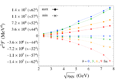
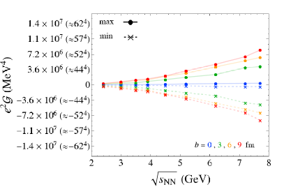
Figure 5: The collision-energy $\sqrt{s_{{}_{\;\!\!N\;\!\!\;\!\!N}}}$ dependence of the maximum (solid) and minimum (dashed) over the spacetime of the Lorentz invariants, ${\mathcal{F}}={\bm{E}}^{2}-{\bm{B}}^{2}$ (left) and ${\mathcal{G}}={\bm{E}}\cdot{\bm{B}}$ (right) for various impact parameters $b$.

To get a quantitative insight, we extract the maximum and minimum values of the Lorentz invariants, ${\mathcal{F}}$ and ${\mathcal{G}}$, over the whole spacetime, and plot them as a function of the collision energy for various values of the impact parameter in Fig. 5.

Fig. 5 indicates that the typical magnitudes of the maxima and minima of ${\mathcal{F}}$ and ${\mathcal{G}}$ are of the order of ${\mathcal{O}}((50\;{\rm MeV})^{4})$. This immediately means that the typical magnitudes of the produced electromagnetic fields, ${\bm{E}}$ and ${\bm{B}}$, are of the order of ${\mathcal{O}}((50\;{\rm MeV})^{2})$. This scale ${\mathcal{O}}(50\;{\rm MeV})^{2}$ is strong in a sense that it goes beyond the critical field strength of QED, $m_{e}^{2}\approx(0.5\;{\rm MeV})^{2}$, and is non-negligibly large even compared to the QCD/hadronic scale $m_{\pi}\approx(140\;{\rm MeV})^{2}$, where $m_{\pi}$ is the pion mass.

The magnitudes of the maxima and minima of ${\mathcal{F}}$ and ${\mathcal{G}}$ are monotonically increasing with the collision energy. In other words, both electric and magnetic fields become stronger, as the collision energy increases. This is essentially because the charge density becomes higher with larger collision energies due to the Lorentz contraction. Note that it does not necessarily mean that high-energy collisions are more advantageous for the observations of strong-field effects. In fact, one must also care about the spacetime volume because it can leave nothing if the spacetime volume is tiny, no matter how strong it is [35]. We will come back to this issue of spacetime in the next subsection.

At the quantitative level, we can numerically fit $\max{\mathcal{F}}$ well with a simple function of the form, ${\rm const}.\times(\sqrt{s_{{}_{\;\!\!N\;\!\!\;\!\!N}}})^{2}$, as

$$\max e^{2}{\mathcal{F}}(b=0\;{\rm fm}) \approx(23\;{\rm MeV})^{4}\times\left(\frac{\sqrt{s_{{}_{\;\!\!N\;\!\!\;\!\!N}}}}{1\;{\rm GeV}}\right)^{2}\;,$$ (8a)

$$\max e^{2}{\mathcal{F}}(b=3\;{\rm fm}) \approx(22\;{\rm MeV})^{4}\times\left(\frac{\sqrt{s_{{}_{\;\!\!N\;\!\!\;\!\!N}}}}{1\;{\rm GeV}}\right)^{2}\;,$$ (8b)

$$\max e^{2}{\mathcal{F}}(b=6\;{\rm fm}) \approx(20\;{\rm MeV})^{4}\times\left(\frac{\sqrt{s_{{}_{\;\!\!N\;\!\!\;\!\!N}}}}{1\;{\rm GeV}}\right)^{2}\;,$$ (8c)

$$\max e^{2}{\mathcal{F}}(b=9\;{\rm fm}) \approx(18\;{\rm MeV})^{4}\times\left(\frac{\sqrt{s_{{}_{\;\!\!N\;\!\!\;\!\!N}}}}{1\;{\rm GeV}}\right)^{2}\;.$$ (8d)

For $\min{\mathcal{F}},\max{\mathcal{G}}$, and $\min{\mathcal{G}}$, we find that the simple function, ${\rm const}.\times(\sqrt{s_{{}_{\;\!\!N\;\!\!\;\!\!N}}})^{2}$, is not sufficient to fit the data but the addition of a constant term makes it working well, ${\rm const}.+{\rm const}.\times(\sqrt{s_{{}_{\;\!\!N\;\!\!\;\!\!N}}})^{2}$. We find

$$\min e^{2}{\mathcal{F}}(b=3\;{\rm fm})$$

$$\quad\approx(21\;{\rm MeV})^{4}-(14\;{\rm MeV})^{4}\times\left(\frac{\sqrt{s_{{}_{\;\!\!N\;\!\!\;\!\!N}}}}{1\;{\rm GeV}}\right)^{2}\;,$$ (9a)

$$\min e^{2}{\mathcal{F}}(b=6\;{\rm fm})$$

$$\quad\approx(29\;{\rm MeV})^{4}-(18\;{\rm MeV})^{4}\times\left(\frac{\sqrt{s_{{}_{\;\!\!N\;\!\!\;\!\!N}}}}{1\;{\rm GeV}}\right)^{2}\;,$$ (9b)

$$\min e^{2}{\mathcal{F}}(b=9\;{\rm fm})$$

$$\quad\approx(35\;{\rm MeV})^{4}-(22\;{\rm MeV})^{4}\times\left(\frac{\sqrt{s_{{}_{\;\!\!N\;\!\!\;\!\!N}}}}{1\;{\rm GeV}}\right)^{2}\;.$$ (9c)

and

$$\max e^{2}{\mathcal{G}}(b=3\;{\rm fm})\approx-\min e^{2}{\mathcal{G}}(b=3\;{\rm fm})$$

$$\quad\approx(-25\;{\rm MeV})^{4}+(17\;{\rm MeV})^{4}\times\left(\frac{\sqrt{s_{{}_{\;\!\!N\;\!\!\;\!\!N}}}}{1\;{\rm GeV}}\right)^{2}\;,$$ (10a)

$$\max e^{2}{\mathcal{G}}(b=6\;{\rm fm})\approx-\min e^{2}{\mathcal{G}}(b=6\;{\rm fm})$$

$$\quad\approx(-25\;{\rm MeV})^{4}+(19\;{\rm MeV})^{4}\times\left(\frac{\sqrt{s_{{}_{\;\!\!N\;\!\!\;\!\!N}}}}{1\;{\rm GeV}}\right)^{2}\;,$$ (10b)

$$\max e^{2}{\mathcal{G}}(b=9\;{\rm fm})\approx-\min e^{2}{\mathcal{G}}(b=9\;{\rm fm})$$

$$\quad\approx(-28\;{\rm MeV})^{4}+(20\;{\rm MeV})^{4}\times\left(\frac{\sqrt{s_{{}_{\;\!\!N\;\!\!\;\!\!N}}}}{1\;{\rm GeV}}\right)^{2}\;,$$ (10c)

where $b=0\;{\rm fm}$ is omitted, for which $\min{\mathcal{F}},\max{\mathcal{G}}$, and $\min{\mathcal{G}}$ are simply vanishing within the residual event-by-event fluctuations.

III.4 Spacetime volume

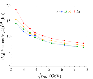
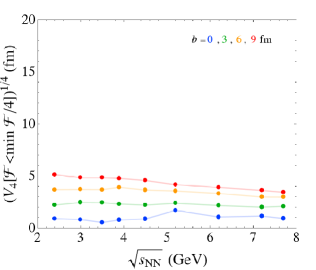
Figure 6: The spacetime four volume $V_{4}$ of the Lorentz invariant ${\mathcal{F}}={\bm{E}}^{2}-{\bm{B}}^{2}$, defined as the region that satisfies ${\mathcal{F}}>\max{\mathcal{F}}/4$ (top) and ${\mathcal{F}}<\min{\mathcal{F}}/4$ (bottom).

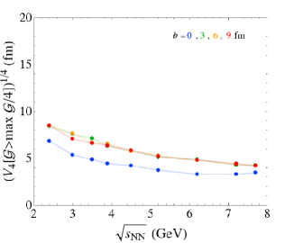
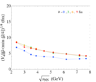
Figure 7: A similar plot to Fig. 6, showing the spacetime four volume $V_{4}$ of the Lorentz invariant ${\mathcal{G}}={\bm{E}}\cdot{\bm{B}}$, defined as the region such that ${\mathcal{G}}>\max{\mathcal{G}}/4$ (top) and ${\mathcal{G}}<\min{\mathcal{G}}/4$ (bottom).

Finally, we quantitatively discuss the spacetime volume of the produced electromagnetic field. We measure the volume by the region that satisfies some threshold conditions. We consider four thresholds and, accordingly, define four kinds of spacetime volumes $V_{4}$ as

$$V_{4}[{\mathcal{F}}>\max{\mathcal{F}}/4]:=\int_{{\mathcal{F}}>\max{\mathcal{F}}/4}{\rm d}^{4}x\;,$$ (11a)

$$V_{4}[{\mathcal{F}}<\min{\mathcal{F}}/4]:=\int_{{\mathcal{F}}<\min{\mathcal{F}}/4}{\rm d}^{4}x\;,$$ (11b)

$$V_{4}[{\mathcal{G}}>\max{\mathcal{G}}/4]:=\int_{{\mathcal{G}}>\max{\mathcal{F}}/4}{\rm d}^{4}x\;,$$ (11c)

$$V_{4}[{\mathcal{G}}<\min{\mathcal{G}}/4]:=\int_{{\mathcal{G}}<\min{\mathcal{F}}/4}{\rm d}^{4}x\;,$$ (11d)

where $\max$ and $\min$ mean to take the maximum and minimum over the whole spacetime, respectively. The physical meaning of these volumes are evident. For example, $V_{4}[{\mathcal{F}}>\max{\mathcal{F}}/4]$ and $V_{4}[{\mathcal{F}}<\min{\mathcal{F}}/4]$, respectively, measure the volumes of the strong electric- and magnetic-field regions such that ${\mathcal{F}}>\max{\mathcal{F}}/4\approx\max{\bm{E}}^{2}/4$ and ${\mathcal{F}}<\min{\mathcal{F}}/4\approx-\max{\bm{B}}^{2}/4$. Note that ${\mathcal{F}}$ and ${\mathcal{G}}$ are roughly the squares of the electromagnetic fields, ${\bm{E}}$ and ${\bm{B}}$, and hence the denominators “4” amounts to consider the half maxima of ${\bm{E}}$ and ${\bm{B}}$.

The results are shown in Fig. 6 for ${\mathcal{F}}$ and in Fig. 7 for ${\mathcal{G}}$. We first observe that the typical magnitude of $V_{4}$ is much larger in the top panel of Fig. 6 compared to the other three panels, i.e., $V_{4}[{\mathcal{F}}>\max{\mathcal{F}}/4]\gg V_{4}[({\rm others})]$. This reflects the fact that the electric field occupies majority of the spacetime, as we have seen in Fig. LABEL:fig:1. It is remarkable that even at the most non-central case $b=9\;{\rm fm}$, we find $V_{4}[{\mathcal{F}}>\max{\mathcal{F}}/4]\approx(10\;{\rm fm})^{4}\gg V_{4}[{\mathcal{F}}<\min{\mathcal{F}}/4]\approx(5\;{\rm fm})^{4}$. In other words, the region dominated by the magnetic field $V_{4}[{\mathcal{F}}<\min{\mathcal{F}}/4]$ is always smaller than that dominated by the electric field $V_{4}[{\mathcal{F}}>\max{\mathcal{F}}/4]$ in intermediate-energy heavy-ion collisions.

Among the four $V_{4}$’s, we find that $V_{4}[{\mathcal{F}}>\max{\mathcal{F}}/4]$ has the strongest collision energy dependence. It scales with $1/\sqrt{s_{{}_{\;\!\!N\;\!\!\;\!\!N}}}$ due to the Lorentz contraction. Quantitatively, we can fit $V_{4}[{\mathcal{F}}>\max{\mathcal{F}}/4]$ well with a function of the form ${\rm const}.+{\rm const.}/\sqrt{s_{{}_{\;\!\!N\;\!\!\;\!\!N}}}$. The numerical coefficients are found to be

$$V_{4}[{\mathcal{F}}>\max{\mathcal{F}}/4](b=0\;{\rm fm})$$

$$\quad\approx(2.7\;{\rm fm})+(27\;{\rm fm})\times\left(\frac{\sqrt{s_{{}_{\;\!\!N\;\!\!\;\!\!N}}}}{1\;{\rm GeV}}\right)^{-1}\;,$$ (12a)

$$V_{4}[{\mathcal{F}}>\max{\mathcal{F}}/4](b=3\;{\rm fm})$$

$$\quad\approx(2.5\;{\rm fm})+(28\;{\rm fm})\times\left(\frac{\sqrt{s_{{}_{\;\!\!N\;\!\!\;\!\!N}}}}{1\;{\rm GeV}}\right)^{-1}\;,$$ (12b)

$$V_{4}[{\mathcal{F}}>\max{\mathcal{F}}/4](b=6\;{\rm fm})$$

$$\quad\approx(2.8\;{\rm fm})+(30\;{\rm fm})\times\left(\frac{\sqrt{s_{{}_{\;\!\!N\;\!\!\;\!\!N}}}}{1\;{\rm GeV}}\right)^{-1}\;,$$ (12c)

$$V_{4}[{\mathcal{F}}>\max{\mathcal{F}}/4](b=9\;{\rm fm})$$

$$\quad\approx(2.3\;{\rm fm})+(37\;{\rm fm})\times\left(\frac{\sqrt{s_{{}_{\;\!\!N\;\!\!\;\!\!N}}}}{1\;{\rm GeV}}\right)^{-1}\;.$$ (12d)

We can apply the same function to fit the other $V_{4}$’s. We find (we omit the uninterested $b=0$ case)

$$V_{4}[{\mathcal{F}}<\min{\mathcal{F}}/4](b=3\;{\rm fm})$$

$$\quad\approx(2.0\;{\rm fm})+(0.88\;{\rm fm})\times\left(\frac{\sqrt{s_{{}_{\;\!\!N\;\!\!\;\!\!N}}}}{1\;{\rm GeV}}\right)^{-1}\;,$$ (13a)

$$V_{4}[{\mathcal{F}}<\min{\mathcal{F}}/4](b=6\;{\rm fm})$$

$$\quad\approx(2.9\;{\rm fm})+(2.5\;{\rm fm})\times\left(\frac{\sqrt{s_{{}_{\;\!\!N\;\!\!\;\!\!N}}}}{1\;{\rm GeV}}\right)^{-1}\;,$$ (13b)

$$V_{4}[{\mathcal{F}}<\min{\mathcal{F}}/4](b=9\;{\rm fm})$$

$$\quad\approx(2.3\;{\rm fm})+(5.9\;{\rm fm})\times\left(\frac{\sqrt{s_{{}_{\;\!\!N\;\!\!\;\!\!N}}}}{1\;{\rm GeV}}\right)^{-1}\;,$$ (13c)

and

$$V_{4}[{\mathcal{G}}>\max{\mathcal{G}}/4](b=3\;{\rm fm})\approx V_{4}[{\mathcal{G}}<\min{\mathcal{G}}/4](b=3\;{\rm fm})$$

$$\quad\approx(2.2\;{\rm fm})+(15\;{\rm fm})\times\left(\frac{\sqrt{s_{{}_{\;\!\!N\;\!\!\;\!\!N}}}}{1\;{\rm GeV}}\right)^{-1}\;,$$ (14a)

$$V_{4}[{\mathcal{G}}>\max{\mathcal{G}}/4](b=6\;{\rm fm})\approx V_{4}[{\mathcal{G}}<\min{\mathcal{G}}/4](b=6\;{\rm fm})$$

$$\quad\approx(2.3\;{\rm fm})+(15\;{\rm fm})\times\left(\frac{\sqrt{s_{{}_{\;\!\!N\;\!\!\;\!\!N}}}}{1\;{\rm GeV}}\right)^{-1}\;,$$ (14b)

$$V_{4}[{\mathcal{G}}>\max{\mathcal{G}}/4](b=9\;{\rm fm})\approx V_{4}[{\mathcal{G}}<\min{\mathcal{G}}/4](b=9\;{\rm fm})$$

$$\quad\approx(2.4\;{\rm fm})+(15\;{\rm fm})\times\left(\frac{\sqrt{s_{{}_{\;\!\!N\;\!\!\;\!\!N}}}}{1\;{\rm GeV}}\right)^{-1}\;.$$ (14c)

It is interesting that $V_{4}$ appears to be insensitive to the impact parameter for ${\mathcal{G}}$, which we do not have a simple explanation.

IV Summary

We have numerically estimated the electromagnetic field produced in intermediate-energy heavy-ion collisions with finite impact parameter, by using a hadron transport model JAM.

Our main findings are (1) that the produced electromagnetic field is strong $eE,eB={\mathcal{O}}((50\;{\rm MeV})^{2})$, which goes beyond the critical field strength of QED, $m_{e}^{2}\approx(0.5\;{\rm MeV})^{2}$, and is non-negligibly large even compared to the QCD/hadronic scale $m_{\pi}^{2}\approx(140\;{\rm MeV})^{2}$; (2) that the produced fields extend in spacetime about $V_{4}={\mathcal{O}}((10\;{\rm fm})^{4})$, which is larger than the typical spacetime volume of the fireball created in heavy-ion collisions [24] and is also large in terms of the nonlinearity parameters of QED [48, 35, 37]; (3) that the majority of the spacetime is occupied by the electric field and the magnetic field dominates only around the collision point; and (4) that a topological electromagnetic-field configuration such that ${\bm{E}}\cdot{\bm{B}}\neq 0$ is realized, which may induce nontrivial chiral phenomena such as chirality production [49, 50, 51, 52] and chiral plasma instability [53].

Our results represent a first step toward quantifying electromagnetic-field effects in intermediate-energy heavy-ion collisions. The next step is to use the electromagnetic-field profile obtained in this study as input for predicting nontrivial observable signatures, such as the dilepton production in the low-momentum regime and the charged directed flow. We leave this for future work.

Appendix A Spacetime profile of electric and magnetic fields

In the main text, we have focused on the spacetime evolution of the electromagnetic Lorentz invariants, ${\mathcal{F}}$ and ${\mathcal{G}}$, rather than each of the electric and magnetic components, ${\bm{E}}$ and ${\bm{B}}$, in order to make the figures and discussions simpler. Here, for interested readers, we display the correspondence of Fig. LABEL:fig:1 for ${\bm{E}}$ and ${\bm{B}}$.

References

- Hattori and Huang [2017] K. Hattori and X.-G. Huang, Novel quantum phenomena induced by strong magnetic fields in heavy-ion collisions, Nucl. Sci. Tech. 28, 26 (2017), arXiv:1609.00747 [nucl-th] .
- Voronyuk et al. [2011] V. Voronyuk, V. D. Toneev, W. Cassing, E. L. Bratkovskaya, V. P. Konchakovski, and S. A. Voloshin, (Electro-)Magnetic field evolution in relativistic heavy-ion collisions, Phys. Rev. C 83, 054911 (2011), arXiv:1103.4239 [nucl-th] .
- Bzdak and Skokov [2012] A. Bzdak and V. Skokov, Event-by-event fluctuations of magnetic and electric fields in heavy ion collisions, Phys. Lett. B 710, 171 (2012), arXiv:1111.1949 [hep-ph] .
- Deng and Huang [2012] W.-T. Deng and X.-G. Huang, Event-by-event generation of electromagnetic fields in heavy-ion collisions, Phys. Rev. C 85, 044907 (2012), arXiv:1201.5108 [nucl-th] .
- Tuchin [2010] K. Tuchin, Synchrotron radiation by fast fermions in heavy-ion collisions, Phys. Rev. C 82, 034904 (2010), [Erratum: Phys.Rev.C 83, 039903 (2011)], arXiv:1006.3051 [nucl-th] .
- McLerran and Skokov [2014] L. McLerran and V. Skokov, Comments About the Electromagnetic Field in Heavy-Ion Collisions, Nucl. Phys. A 929, 184 (2014), arXiv:1305.0774 [hep-ph] .
- Gursoy et al. [2014] U. Gursoy, D. Kharzeev, and K. Rajagopal, Magnetohydrodynamics, charged currents and directed flow in heavy ion collisions, Phys. Rev. C 89, 054905 (2014), arXiv:1401.3805 [hep-ph] .
- Tuchin [2016] K. Tuchin, Initial value problem for magnetic fields in heavy ion collisions, Phys. Rev. C 93, 014905 (2016), arXiv:1508.06925 [hep-ph] .
- Li et al. [2016] H. Li, X.-l. Sheng, and Q. Wang, Electromagnetic fields with electric and chiral magnetic conductivities in heavy ion collisions, Phys. Rev. C 94, 044903 (2016), arXiv:1602.02223 [nucl-th] .
- Stewart and Tuchin [2021] E. Stewart and K. Tuchin, Continuous evolution of electromagnetic field in heavy-ion collisions, Nucl. Phys. A 1016, 122308 (2021), arXiv:2106.09124 [nucl-th] .
- Kharzeev et al. [2008] D. E. Kharzeev, L. D. McLerran, and H. J. Warringa, The Effects of topological charge change in heavy ion collisions: ’Event by event P and CP violation’, Nucl. Phys. A 803, 227 (2008), arXiv:0711.0950 [hep-ph] .
- Fukushima et al. [2008] K. Fukushima, D. E. Kharzeev, and H. J. Warringa, The Chiral Magnetic Effect, Phys. Rev. D 78, 074033 (2008), arXiv:0808.3382 [hep-ph] .
- Andersen et al. [2016] J. O. Andersen, W. R. Naylor, and A. Tranberg, Phase diagram of QCD in a magnetic field: A review, Rev. Mod. Phys. 88, 025001 (2016), arXiv:1411.7176 [hep-ph] .
- D’Elia et al. [2022] M. D’Elia, L. Maio, F. Sanfilippo, and A. Stanzione, Phase diagram of QCD in a magnetic background, Phys. Rev. D 105, 034511 (2022), arXiv:2111.11237 [hep-lat] .
- Adhikari et al. [2024] P. Adhikari et al., Strongly interacting matter in extreme magnetic fields, (2024), arXiv:2412.18632 [nucl-th] .
- Di Piazza et al. [2012] A. Di Piazza, C. Muller, K. Z. Hatsagortsyan, and C. H. Keitel, Extremely high-intensity laser interactions with fundamental quantum systems, Rev. Mod. Phys. 84, 1177 (2012), arXiv:1111.3886 [hep-ph] .
- Fedotov et al. [2023] A. Fedotov, A. Ilderton, F. Karbstein, B. King, D. Seipt, H. Taya, and G. Torgrimsson, Advances in QED with intense background fields, Phys. Rept. 1010, 1 (2023), arXiv:2203.00019 [hep-ph] .
- Aaboud et al. [2017] M. Aaboud et al. (ATLAS), Evidence for light-by-light scattering in heavy-ion collisions with the ATLAS detector at the LHC, Nature Phys. 13, 852 (2017), arXiv:1702.01625 [hep-ex] .
- Adam et al. [2021] J. Adam et al. (STAR), Measurement of Momentum and Angular Distributions from Linearly Polarized Photon Collisions, Phys. Rev. Lett. 127, 052302 (2021), arXiv:1910.12400 [nucl-ex] .
- Brandenburg et al. [2023] J. D. Brandenburg, J. Seger, Z. Xu, and W. Zha, Report on progress in physics: observation of the Breit–Wheeler process and vacuum birefringence in heavy-ion collisions, Rept. Prog. Phys. 86, 083901 (2023), arXiv:2208.14943 [hep-ph] .
- Gürsoy et al. [2018] U. Gürsoy, D. Kharzeev, E. Marcus, K. Rajagopal, and C. Shen, Charge-dependent Flow Induced by Magnetic and Electric Fields in Heavy Ion Collisions, Phys. Rev. C 98, 055201 (2018), arXiv:1806.05288 [hep-ph] .
- Abdulhamid et al. [2024] M. I. Abdulhamid et al. (STAR), Observation of the electromagnetic field effect via charge-dependent directed flow in heavy-ion collisions at the Relativistic Heavy Ion Collider, Phys. Rev. X 14, 011028 (2024), arXiv:2304.03430 [nucl-ex] .
- Dash [2024] A. P. Dash, Exploring Electromagnetic Field Effects and Constraining Transport Parameters of QGP using STAR BES-II data, (2024), arXiv:2401.04838 [nucl-ex] .
- Taya et al. [2024a] H. Taya, A. Jinno, M. Kitazawa, and Y. Nara, Optimal collision energy for realizing macroscopic high baryon-density matter, (2024a), arXiv:2409.07685 [hep-ph] .
- Aparin [2023] A. Aparin (STAR Collaboration), STAR Experiment Results From Beam Energy Scan Program, Phys. Atom. Nucl. 86, 758 (2023).
- NA [6] https://shine.web.cern.ch/.
- [27] https://nica.jinr.ru/.
- [28] https://fair-center.de/.
- [29] https://english.imp.cas.cn/research/facilities/HIAF/.
- [30] https://asrc.jaea.go.jp/soshiki/gr/hadron/jparc-hi/index.html.
- Galatyuk [2019] T. Galatyuk, Future facilities for high physics, Nucl. Phys. A 982, 163 (2019).
- Ou and Li [2011] L. Ou and B.-A. Li, Magnetic effects in heavy-ion collisions at intermediate energies, Phys. Rev. C 84, 064605 (2011), arXiv:1107.3192 [nucl-th] .
- Sun et al. [2019] Y. Sun, Y. Wang, Q. Li, and F. Wang, Effect of internal magnetic field on collective flow in heavy ion collisions at intermediate energies, Phys. Rev. C 99, 064607 (2019), arXiv:1905.12492 [nucl-th] .
- Wei et al. [2021] G.-F. Wei, C. Liu, X.-W. Cao, Q.-J. Zhi, W.-J. Xiao, C.-Y. Long, and Z.-W. Long, Necessity of self-consistent calculations for the electromagnetic field in probing the nuclear symmetry energy using pion observables in heavy-ion collisions, Phys. Rev. C 103, 054607 (2021), arXiv:2105.01866 [nucl-th] .
- Taya et al. [2024b] H. Taya, T. Nishimura, and A. Ohnishi, Estimation of electric field in intermediate-energy heavy-ion collisions, Phys. Rev. C 110, 014901 (2024b), arXiv:2402.17136 [hep-ph] .
- Panda et al. [2024] A. K. Panda, P. Bagchi, H. Mishra, and V. Roy, Electromagnetic fields in low-energy heavy-ion collisions with baryon stopping, Phys. Rev. C 110, 024902 (2024), arXiv:2404.08431 [nucl-th] .
- Siddique et al. [2025] I. Siddique, A. Huang, M. Huang, and M. A. Wasaye, Dynamical Electromagnetic fields and Dynamical Electromagnetic Anomaly in heavy ion collisions at intermediate energies (2025), arXiv:2501.11328 [nucl-th] .
- Nishimura et al. [2022] T. Nishimura, M. Kitazawa, and T. Kunihiro, Anomalous enhancement of dilepton production as a precursor of color superconductivity, PTEP 2022, 093D02 (2022), arXiv:2201.01963 [hep-ph] .
- Savchuk et al. [2023] O. Savchuk, A. Motornenko, J. Steinheimer, V. Vovchenko, M. Bleicher, M. Gorenstein, and T. Galatyuk, Enhanced dilepton emission from a phase transition in dense matter, J. Phys. G 50, 125104 (2023), arXiv:2209.05267 [nucl-th] .
- Nishimura et al. [2023a] T. Nishimura, M. Kitazawa, and T. Kunihiro, Enhancement of dilepton production rate and electric conductivity around the QCD critical point, PTEP 2023, 053D01 (2023a), arXiv:2302.03191 [hep-ph] .
- Nishimura et al. [2023b] T. Nishimura, Y. Nara, and J. Steinheimer, Enhanced Dilepton production near the color superconducting phase and the QCD critical point, (2023b), arXiv:2311.14135 [hep-ph] .
- Yoon et al. [2021] J. W. Yoon, Y. G. Kim, I. W. Choi, J. H. Sung, H. W. Lee, S. K. Lee, and C. H. Nam, Realization of laser intensity over , Optica 8, 630 (2021).
- [43] The white paper of ELI can be find at https://www.eli-np.ro/whitebook.php.
- Nara et al. [2000] Y. Nara, N. Otuka, A. Ohnishi, K. Niita, and S. Chiba, Study of relativistic nuclear collisions at AGS energies from p + Be to Au + Au with hadronic cascade model, Phys. Rev. C 61, 024901 (2000), arXiv:nucl-th/9904059 .
- [45] The latest version of JAM (JAM2) is publically available at https://gitlab.com/transportmodel/jam2.
- Wolter et al. [2022] H. Wolter et al. (TMEP), Transport model comparison studies of intermediate-energy heavy-ion collisions, Prog. Part. Nucl. Phys. 125, 103962 (2022), arXiv:2202.06672 [nucl-th] .
- Deng et al. [2020] X.-G. Deng, X.-G. Huang, Y.-G. Ma, and S. Zhang, Vorticity in low-energy heavy-ion collisions, Phys. Rev. C 101, 064908 (2020), arXiv:2001.01371 [nucl-th] .
- Taya et al. [2014] H. Taya, H. Fujii, and K. Itakura, Finite pulse effects on pair creation from strong electric fields, Phys. Rev. D 90, 014039 (2014), arXiv:1405.6182 [hep-ph] .
- Fukushima et al. [2010] K. Fukushima, D. E. Kharzeev, and H. J. Warringa, Real-time dynamics of the Chiral Magnetic Effect, Phys. Rev. Lett. 104, 212001 (2010), arXiv:1002.2495 [hep-ph] .
- Warringa [2012] H. J. Warringa, Dynamics of the Chiral Magnetic Effect in a weak magnetic field, Phys. Rev. D 86, 085029 (2012), arXiv:1205.5679 [hep-th] .
- Copinger et al. [2018] P. Copinger, K. Fukushima, and S. Pu, Axial Ward identity and the Schwinger mechanism – Applications to the real-time chiral magnetic effect and condensates, Phys. Rev. Lett. 121, 261602 (2018), arXiv:1807.04416 [hep-th] .
- Taya [2020] H. Taya, Dynamically assisted Schwinger mechanism and chirality production in parallel electromagnetic field, Phys. Rev. Res. 2, 023257 (2020), arXiv:2003.08948 [hep-ph] .
- Akamatsu and Yamamoto [2013] Y. Akamatsu and N. Yamamoto, Chiral Plasma Instabilities, Phys. Rev. Lett. 111, 052002 (2013), arXiv:1302.2125 [nucl-th] .