Faster Convergence of Riemannian Stochastic Gradient Descent
with Increasing Batch Size

Abstract

Many models used in machine learning have become so large that even computer computation of the full gradient of the loss function is impractical. This has made it necessary to efficiently train models using limited available information, such as batch size and learning rate. We have theoretically analyzed the use of Riemannian stochastic gradient descent (RSGD) and found that using an increasing batch size leads to faster RSGD convergence than using a constant batch size not only with a constant learning rate but also with a decaying learning rate, such as cosine annealing decay and polynomial decay. In particular, RSGD has a better convergence rate $O(\frac{1}{\sqrt{T}})$ than the existing rate $O(\frac{\sqrt{\log T}}{\sqrt[4]{T}})$ with a diminishing learning rate, where $T$ is the number of iterations. The results of experiments on principal component analysis and low-rank matrix completion problems confirmed that, except for the MovieLens dataset and a constant learning rate, using a polynomial growth batch size or an exponential growth batch size results in better performance than using a constant batch size.

1 Introduction

Reference and Theorem	Additional Assumption(s)	Batch Size	Learning Rate	Convergence Analysis
Bonnabel (2013)	Several	–	s.a.r.	$\underset{t\to\infty}{\lim}\mathbb{E}[\mathrm{grad}f(x_{t})]=0\text{ a.s.}$
Zhang & Sra (2016)	Several	–	$\eta_{t}=O(\frac{1}{L_{r}+\sqrt{t}})$	$\mathbb{E}[f(\bar{x}_{T})-f^{\star}]=O(\frac{\sqrt{T}}{C+T})$
Tripuraneni et al. (2018)	Several	Constant	$\eta_{t}=O(\frac{1}{t^{\alpha}})$	$\mathbb{E}\|\tilde{\Delta}_{T}\|=O(\frac{1}{\sqrt{T}})$
Hosseini & Sra (2020)	Bounded Gradient	Constant	$\eta_{t}=O(\frac{1}{\sqrt{T}})$	$\mathbb{E}\|\mathrm{grad}f(x_{T})\|=O(\frac{1}{\sqrt[4]{T}})$
Durmus et al. (2021)	Several	Constant	Constant	$\mathbb{E}[f(x_{T})-f^{\star}]=O(C_{1}^{T}+C_{2})$
Sakai & Iiduka (2024)	Several	Constant	$\eta_{t}=\frac{1}{\sqrt{t+1}}$	$\mathbb{E}\|\mathrm{grad}f(x_{T})\|=O(\frac{\sqrt{\log T}}{\sqrt[4]{T}})$
Sakai & Iiduka (2025)	Bounded Gradient	Increasing	Constant	$\mathbb{E}\|\mathrm{grad}f(x_{T})\|=O(\frac{1}{\sqrt{T}})$
Theorem 4.1	–	Constant	Constant and Decay	$\mathbb{E}\|\mathrm{grad}f(x_{T})\|=O(\sqrt{\frac{1}{T}+C})$
Theorem 4.2	–	Increasing	Constant and Decay	$\mathbb{E}\|\mathrm{grad}f(x_{T})\|=O(\frac{1}{\sqrt{T}})$
Theorem 4.3	–	Increasing	Warm-up	$\mathbb{E}\|\mathrm{grad}f(x_{T})\|=O(\frac{1}{\sqrt{T-T_{w}}})$
Theorem 4.4	–	Constant	Warm-up	$\mathbb{E}\|\mathrm{grad}f(x_{T})\|=O(\sqrt{\frac{1}{T-T_{w}}+C})$

Table 1: Comparison of RSGD convergence analyses, where $\alpha\in(\frac{1}{2},1),C_{1}\in(0,1),C_{2}$ and $C$ are constants. For $\tilde{x}_{t}\coloneq R_{\tilde{x}_{t-1}}(\frac{1}{t}R_{\tilde{x}_{t-1}}^{-1}(x_{t}))$, $\tilde{\Delta}_{t}\coloneq R_{x^{\star}}^{-1}(\tilde{x}_{t})$. In particular, $\bar{x}_{t}$ denotes $\tilde{x}_{t}$ with $R\coloneq\mathrm{Exp}$. In Euclidean space, $\tilde{x}_{t}$ is represented by $\tilde{x}_{t}:=\tilde{x}_{t-1}+\frac{1}{t}(x_{t}-\tilde{x}_{t-1})$ (see Tripuraneni et al. (2018) for details). The usual stochastic approximation learning rate rule (s.a.r.) is defined as $\sum_{t=0}^{\infty}\eta_{t}=\infty,\sum_{t=0}^{\infty}\eta_{t}^{2}<\infty$ (Robbins & Monro, 1951). $T$ is the total number of iterations, and $T_{w}$ is the number of warm-up iterations (see Section 4.3). The upper bound of $\min_{t\in\{0,\cdots,T-1\}}\mathbb{E}[\|\mathrm{grad}f(x_{t})\|_{x_{t}}]$ is represented by $\mathbb{E}\|\mathrm{grad}f(x_{T})\|$ or $\|G_{T}\|$.

Stochastic gradient descent (SGD) (Robbins & Monro, 1951) is a basic algorithm in stochastic optimization theory. It and its derivations are widely used in machine learning (Liu et al., 2021; He et al., 2016; Krizhevsky et al., 2012). Riemannian stochastic gradient descent (RSGD) was proposed in Bonnabel (2013). RSGD is the algorithm on a Riemannian manifold corresponding to SGD on a Euclidean space. Riemannian optimization (Absil et al., 2008; Boumal, 2023), which studies RSGD and its derivations, has been attracting attention for its use in many machine learning tasks. For example, it has been used in principal components analysis (Breloy et al., 2021; Liu & Boumal, 2020; Roy et al., 2018), low-rank matrix completion (Vandereycken, 2013; Nguyen et al., 2019; Boumal & Absil, 2015; Kasai & Mishra, 2016), convolutional neural networks (Wang et al., 2020; Huang et al., 2017; Chen et al., 2017), graph neural networks (Zhu et al., 2020; Chami et al., 2019; Liu et al., 2019), and language model tasks (Bécigneul & Ganea, 2019; Yun & Yang, 2023) and has been used in applications of optimal transportation theory (Lin et al., 2020a; Weber & Sra, 2023) and applications of computer vision (Chen et al., 2024; He et al., 2024). An advantage of Riemannian optimization is that notions difficult to handle in Euclidean space are easier to treat. For example, there exists a nonconvex function on a Euclidean space that becomes geodesically convex on a Riemannian manifold (Zhang & Sra, 2016; Hu et al., 2020; Fei et al., 2023; Zhang et al., 2016). Note that the notion of geodesically convex functions corresponds to the notion of convex functions in Euclidean space, so we can use the convex function paradigm for several nonconvex functions. This advantage has been applied to nonconvex problems (e.g., Cai et al. (2022); Wang et al. (2020); Sun et al. (2017); Vandereycken (2013); Hosseini & Sra (2015); Liu et al. (2015)). Another example is that there exists a constrained optimization problem in Euclidean space that becomes an unconstrained optimization problem in Riemannian manifold (Boumal, 2023; Hu et al., 2020; Fei et al., 2023). By utilizing the geometric structure of manifolds in optimization, additional useful results can be obtained (see Fei et al. (2023) for details).

However, Riemannian optimization is relatively unexplored compared with Euclidean optimization. Since the models used in many machine learning tasks are huge, computing the full gradient of the loss function can be difficult, which makes it necessary to efficiently train models using limited available information. Therefore, the batch size (BS) and learning rate (LR) are important RSGD settings for the efficient training. In previous work by Ji et al. (2023); Bonnabel (2013); Kasai et al. (2019, 2018); Sakai & Iiduka (2024), the BS was treated as a constant, while in previous work by Sakai & Iiduka (2025); Han & Gao (2022), it was treated as adaptive (although the latter did not treat RSGD). Sato & Iiduka (2024); Keskar et al. (2017); Lin et al. (2020b); McCandlish et al. (2018); You et al. (2020); Hoffer et al. (2017) found that, in the Euclidean case, using a large constant BS led to a poor minima. Sato & Iiduka (2024) found that using an increasing BS or a decaying LR led to a better minima, and Umeda & Iiduka (2024) found that it accelerated the convergence of SGD. Inspired by these findings, we have developed a faster convergence rate of RSGD with an increasing BS and several types of a decaying LR that have not been analyzed for Riemannian optimization. Many decaying LR types have been devised, including cosine annealing (Loshchilov & Hutter, 2017), polynomial decay (Chen et al., 2018), cosine power annealing (Hundt et al., 2019), exponential decay (Wu et al., 2014), ABEL (Lewkowycz, 2021), and linear decay (Liu et al., 2020).

1.1 Previous Results and Contributions

Table 1 summarizes the settings and results of convergence analysis of previous theoretical studies on RSGD. Bonnabel (2013); Zhang & Sra (2016); Durmus et al. (2021); Sakai & Iiduka (2024) used a Riemannian manifold with certain conditions for their analyses while Sakai & Iiduka (2024) used an Hadamard manifold, which is a complete simply connected Riemannian manifold with non-positive sectional curvature. Durmus et al. (2021) used a constrained set, which is a subset of an Hadamard manifold that is closed geodesically convex with a nonempty interior. Therefore, their condition was tighter than Sakai & Iiduka (2024). Bonnabel (2013) performed convergence analyses on a Riemannian manifold with a bounded diameter and the similar proposition with this on an Hadamard manifold. Zhang & Sra (2016) used the same conditions appear in Bonnabel (2013). An Hadamard manifold is important for using an exponential map as a retraction since the manifold ensures the existence of an inverse exponential map (the Cartan-Hadamard theorem). Our condition contains an Hadamard manifold as one example. Whereas Zhang & Sra (2016); Tripuraneni et al. (2018); Durmus et al. (2021); Sakai & Iiduka (2025) assumed the existence of the Hessian with certain conditions or bounded gradient condition, our analyses did not. Furthermore, our analyses contain strongly convex objective function and smooth retraction, which is often used (see Section 2 for details). Most of the studies listed in Table 1 treat used a constant BS and a constant or diminishing type LR. Tripuraneni et al. (2018) achieved a convergence rate of $O(\frac{1}{\sqrt{T}})$; however, they assumed tight conditions, as described above. Hosseini & Sra (2020) achieved a convergence rate of $O(\frac{1}{\sqrt[4]{T}})$ using assumptions more general than Tripuraneni et al. (2018); however, using the constant LR $\eta_{t}=O(\frac{1}{\sqrt{T}})$ needs to set the number of iterations $T$ before implementing RSGD. Since we cannot diverge the $T$, the upper bound $O(\frac{1}{\sqrt[4]{T}})$ in Hosseini & Sra (2020) cannot converge to $0$. Sakai & Iiduka (2025) used an increasing BS and a constant or diminishing LR and achieved $O(\frac{1}{\sqrt{T}})$ under more general conditions than in the other previous studies listed in Table 1. Our analyses achieved $O(\frac{1}{\sqrt{T}})$ without using tight conditions including the bounded gradient condition and with using a cosine annealing LR, a polynomial decay LR, and warm-up LRs that were not analyzed in previous work. Furthermore, the BSs we used are applicable to many useful and practical examples (see Section 4). Our study has three main novelties.

• We used not only a constant BS but also an increasing BS and demonstrated that using an increasing BS leads to faster convergence of RSGD. With a diminishing LR (2), a convergence rate of $O(\frac{\sqrt{\log T}}{\sqrt[4]{T}})$ can be achieved with a constant BS (Theorem 4.1), whereas a convergence rate of $O(\frac{1}{\sqrt[4]{T}})$ can be achieved with an increasing BS (Theorem 4.2). Moreover, with the other LRs (1), (3) and (4), a convergence rate of $O(\sqrt{\frac{1}{T}+\frac{\sigma^{2}}{b}})$ can be achieved with a constant BS (Theorem 4.1), a convergence rate of $O(\frac{1}{\sqrt{T}})$ can be achieved with an increasing BS (Theorem 4.2). Additionally, even with a warm-up LR, using an increasing BS (Theorem 4.3) results in a better convergence rate than using a constant BS (Theorem 4.4).

• Using a more general assumption than in the previous studies listed in Table 1, we achieved a convergence rate of $O(\frac{1}{\sqrt{T}})$ with decaying type LRs that were not used in previous analyses, including a cosine annealing LR (3) and a polynomial decay LR (4), as well as with a warm-up LR (see Section 4.3). Furthermore, we also used a constant LR (1) and a diminishing LR (2).

• Our analyses of using constant and increasing BSs and several LR types should serve as a theoretical framework for RSGD. Additionally, our numerical results in Section 5 support our convergence analyses.

The intuition for why an increasing BS leads to faster convergence of RSGD: As proven in Theorems 4.1 and 4.4 and by Hosseini & Sra (2020); Sakai & Iiduka (2024, 2025), many convergence analyses have shown that using a constant BS can result in a convergence rate of $O(\sqrt{\frac{1}{T}+\frac{1}{b}})$. Since $\lim_{b\to\infty}b^{-1}=0$, this theoretical result suggests that using an increasing BS improves the RSGD convergence rate. Theorems 4.2 and 4.3 support this intuition.

2 Preliminaries

2.1 Basic Notions for Riemannian Optimization

Let $\mathbb{R}^{d}$ be a $d$ dimensional Euclidean space with $\langle x,y\rangle_{2}\coloneq x^{\top}y$. For a manifold $\mathcal{M}$, $T\mathcal{M}$ denotes the tangent bundle of $\mathcal{M}$, and $T_{x}\mathcal{M}$ denotes the tangent space at $x\in\mathcal{M}$. In particular, when $\mathrm{dim}\mathcal{M}=d$, $T_{x}\mathcal{M}$ equals the vector space spanned by $\{(\frac{\partial}{\partial y_{j}})_{x}\}_{j=1,\ldots,d}$. For a smooth map $F\colon\mathcal{M}\to\mathcal{N}$, we denote the differential of $F$ by $DF$. For all $x\in\mathcal{M}$, we suppose that there exists an inner product $g_{x}\colon T_{x}\mathcal{M}\times T_{x}\mathcal{M}\rightarrow\mathbb{R}$ and define $g(x)\coloneq g_{x}$ $(x\in\mathcal{M})$ as the Riemannian metric. If $g$ is smooth, $(\mathcal{M},g)$ is referred to as a Riemannian manifold. We simply write a Riemannian manifold $(\mathcal{M},g)$ as $\mathcal{M}$. Given that $\mathcal{M}$ is a Riemannian manifold, $T_{x}\mathcal{M}$ has a norm induced by the Riemannian metric: $\|v\|_{x}\coloneq\sqrt{\langle v,v\rangle_{x}}\coloneq\sqrt{g_{x}(v,v)}$ $(v\in T_{x}\mathcal{M})$. For a smooth map $f\colon\mathcal{M}\rightarrow\mathbb{R}$ and each $x\in\mathcal{M}$, we define gradient $\mathrm{grad}f(x)$ as a unique tangent vector that satisfies $\forall v\in T_{x}\mathcal{M}\colon Df(x)v=\langle\mathrm{grad}f(x),v\rangle_{x}$. One can easily observe the existence and uniqueness of $\mathrm{grad}f(x)$ (see Lee (1997)).

Iterative methods in Euclidean space $\mathbb{R}^{d}$ are generally represented in the form $x_{t+1}=x_{t}+\eta_{t}d_{t}$ with LR $\eta_{t}\in\mathbb{R}$ and search direction $d_{t}\in\mathbb{R}^{d}$, where addition on $\mathbb{R}^{d}$ is used to update the points generated by the algorithms. However, Riemannian manifolds are not usually equipped with addition, so a method for updating procedure on Riemannian manifolds needs to be defined.

Definition 2.1 (Retraction).

Let $0_{x}$ be a zero element of $T_{x}\mathcal{M}$. When a map $R\colon T\mathcal{M}\ni(x,v)\mapsto R_{x}(v)\in\mathcal{M}$ satisfies the following conditions, $R$ is referred to as a retraction on $\mathcal{M}$.

1. $R_{x}(0_{x})=x$,

2. With the canonical identification $T_{0_{x}}T_{x}\mathcal{M}\simeq T_{x}\mathcal{M}$, $DR_{x}(0_{x})=\mathrm{id}_{T_{x}\mathcal{M}}$ for all $x\in\mathcal{M}$,

where $\mathrm{id}_{T_{x}\mathcal{M}}\colon T_{x}\mathcal{M}\to T_{x}\mathcal{M}$ is the identity mapping.

For instance, if $\mathcal{M}=\mathbb{R}^{d}$, then $R_{x}(v)\coloneq x+v$ is a retraction on $\mathbb{R}^{d}$ (see Absil et al. (2008, Section 4.1.1)). Hence, the updating procedure in Euclidean space can be rewritten as $x_{t+1}=R_{x_{t}}(\eta_{t}d_{t})$. This means that retractions are an extension of the updating procedure in Euclidean space. Exponential maps are often used as retractions for moving points along the search direction on Riemannian manifolds. The following assumption plays a central role in Lemma 3.1.

Assumption 2.2 (Retraction Smoothness).

Let $f\colon\mathcal{M}\rightarrow\mathbb{R}$ be a smooth map. Then there exists $L_{r}>0$ such that, for all $x\in\mathcal{M}$ and all $v\in T_{x}\mathcal{M}$,

$$f(R_{x}(v))\leq f(x)+\langle\mathrm{grad}f(x),v\rangle_{x}+\frac{L_{r}}{2}\|v\|_{x}^{2}.$$

In the Euclidean space setting, $L$-smoothness implies a property similar to retraction smoothness. The property corresponding to $L$-smoothness in Euclidean space is defined for $f\colon\mathcal{M}\rightarrow\mathbb{R}$ as

$$\exists L>0,\forall x,y\in\mathcal{M}\colon$$

$$\quad\|\mathrm{grad}f(x)-\Gamma^{x}_{y}\mathrm{grad}f(y)\|_{x}\leq Ld(x,y),$$

where $\Gamma$ is the parallel transport from $T_{y}\mathcal{M}$ to $T_{x}\mathcal{M}$, and $d(\cdot,\cdot)$ is the Riemannian distance. This is a necessary condition for Assumption 2.2 with $L_{r}\coloneq L$ and $R\coloneq\mathrm{Exp}$ (see Boumal (2023, Corollary 10.54)). This case is frequently used (e.g., Zhang & Sra (2016); Criscitiello & Boumal (2023); Kim & Yang (2022); Liu et al. (2017)). Other necessary conditions for Assumption 2.2 were identified by Kasai et al. (2018, Lemma 3.5) and Sakai & Iiduka (2025, Proposition 3.2). As with parallel transport, a mapping that transports a tangent vector from one tangent space to another is generally called vector transport (see Absil et al. (2008, Section 8.1) for details).

2.2 Riemannian Stochastic Gradient Descent

In machine learning, an empirical loss function is used as the objective function of an optimization problem. It is represented by

$$f(x)\coloneq\frac{1}{N}\sum_{j=1}^{N}f_{j}(x),$$

where every $f_{j}\colon\mathcal{M}\rightarrow\mathbb{R}$ is a mapping. We suppose that every $f_{j}$ is smooth and lower bounded. Therefore, $f$ satisfies the same conditions. This assumption is often made for both Euclidean space and Riemannian space. The lower boundedness of $f$ is essential for analyses using optimization theory since unbounded $f$ may not have optimizers. We denote an optimizer of $f$ as $x^{\star}$ ($f^{\star}\coloneq f(x^{\star})$) and denote $N$ is the size of a dataset. Since the dimension of model parameters $x$ will be a large number, it is not practical to compute the gradient of $f$ using all data. Hence, the mini batch gradient defined as follows is frequently used.

$$\mathrm{grad}f_{B}(x)\coloneq\frac{1}{b}\sum_{j=1}^{b}\mathrm{grad}f_{\xi_{j}}(x),$$

where $B$ represents a minibatch with size $b$, and $(\xi_{j})_{j}$ is a $\{1,\cdots,N\}$-valued i.i.d. copy. Namely, the gradient of $f_{B}(x)=\frac{1}{b}\sum_{j=1}^{b}f_{\xi_{j}}(x)$ is used instead of $\mathrm{grad}f(x)$. The following assumption is reasonable given this situation.

Assumption 2.3 (Bounded Variance Estimator).

The stochastic gradient given by a distribution $\Pi$ is an unbiased estimator and has a bounded variance:

1. $\forall x\in\mathcal{M}\colon\mathbb{E}_{\xi\sim\Pi}\left[\mathrm{grad}f_{\xi}(x)\right]=\mathrm{grad}f(x)$,

2. $\exists\sigma>0,\forall x\in\mathcal{M}\colon\mathbb{V}_{\xi\sim\Pi}(\mathrm{grad}f_{\xi}(x))\leq\sigma^{2}.$

Remark 2.4.

Note that, from 1, $\mathbb{V}_{\xi\sim\Pi}(\mathrm{grad}f_{\xi}(x))=\mathbb{E}_{\xi\sim\Pi}\left[\|\mathrm{grad}f_{\xi}(x)-\mathrm{grad}f(x)\|_{x}^{2}\right]$ holds.

For example, if $f$ being lower bounded satisfies Assumption 2.2 and one takes the uniform distribution as $\Pi$, then Assumption 2.3 holds. In contrast, as stated in Section 2.1, iterative methods on a Riemannian manifold are generally represented as $x_{t+1}=R_{x_{t}}(\eta_{t}d_{t})$ $(\eta_{t}\geq 0,d_{t}\in T_{x_{t}}\mathcal{M})$. The case in which $d_{t}=-\mathrm{grad}f_{B_{t}}(x_{t})$ corresponds to RSGD (Bonnabel, 2013):

$$x_{t+1}=R_{x_{t}}(-\eta_{t}\mathrm{grad}f_{B_{t}}(x_{t})).$$

Additionally, the case in which $d_{t}=-\mathrm{grad}f(x_{t})$ is said to be gradient descent on a Riemannian manifold. We suppose that the sequence $(x_{t})_{t}$ generated by RSGD is independent of random variables $(\xi_{j,t})_{j,t}$ for the minibatch gradient. Note that the BS $(b_{t})_{t}$ is variable at each step.

2.3 Notations

Let $\mathbb{N}$ be the set of positive integers and $\mathbb{N}_{0}\coloneq\mathbb{N}\cup\{0\}$. For a probability space $(\Omega,\mathcal{F},\mathbb{P})$ and a measurable function $f$, $\mathbb{E}[f]\coloneq\int_{\Omega}fd\mathbb{P}$ and $\mathbb{V}(f)\coloneq\mathbb{E}[(f-\mathbb{E}[f])^{2}]$. In particular, for a distribution $\Pi$ on $(\Omega,\mathcal{F})$, an $\{1,\ldots,N\}$-valued measurable function $\xi$, and $f_{\xi}(x)\coloneq f(x;\xi)$, $\mathbb{E}_{\xi\sim\Pi}[f_{\xi}(x)]$ denotes $\int_{\{1,\ldots,N\}}f_{\xi}(x)\Pi(d\xi)$. We define $\mathcal{F}_{t}\coloneq\sigma[x_{0},(\xi_{j,0})_{j},(\xi_{j,1})_{j},\ldots,(\xi_{j,t-1})_{j}]$, so $(\mathcal{F}_{t})_{t\in\mathbb{N}_{0}}$ becomes a filtration, where $x_{0}$ is the initial point of RSGD. For measurable function $f$, $\mathbb{E}[f|\mathcal{F}_{t}]$ denotes the conditional expectation of $\mathcal{F}_{t}$. $\mathrm{St}(r,n)\coloneq\{U\in\mathbb{R}^{r\times n}\mid U^{\top}U=I_{n}\}(r\leq n)$ becomes a Riemannian manifold called the Stiefel manifold (Tagare, 2011). For $n,r\in\mathbb{N}$ s.t. $r\leq n$, a set of all $r$ dimensional subspaces of $\mathbb{R}^{n}$ becomes a Grassmann manifold, denoted as $\mathrm{Gr}(r,n)$. We define $\sim$ on $\mathbb{R}^{n\times r}$ as $A\sim B:\Leftrightarrow\mathrm{col}A=\mathrm{col}B$, where $\mathrm{col}A$ denotes the vector space spanned by columns of matrix $A$. Then, $\mathrm{Gr}(r,n)$ can be identified with $\mathrm{St}(r,n)/\sim$ (Absil et al., 2008). The definition of $\|G_{T}\|$ is in the caption of Table 1.

3 Underlying Analysis

Lemma 3.2 plays a central role here, and Lemma 3.1 is used in the proof of Lemma 3.2.

Lemma 3.1 (Descent Lemma).

Let $(x_{t})_{t}$ be a sequence generated by RSGD and $(\eta_{t})_{t}$ be a positive valued sequence. Then, under Assumptions 2.2 and 2.3, we obtain

$$\mathbb{E}[f(x_{t+1})] \leq\mathbb{E}[f(x_{t})]+\frac{L_{r}\sigma^{2}\eta_{t}^{2}}{2b_{t}}$$

$$\quad-\eta_{t}\left(1-\frac{L_{r}\eta_{t}}{2}\right)\mathbb{E}[\|\mathrm{grad}f(x_{t})\|_{x_{t}}^{2}].$$

Lemma 3.1 implies the following lemma. The proofs of both lemmas are given in Appendices A.1 and A.2.

Lemma 3.2 (Underlying Analysis).

Let $(x_{t})_{t}$ be a sequence generated by RSGD and $\eta_{\max}>0$. We consider a positive valued sequence $(\eta_{t})_{t}$ such that $\eta_{t}\in[0,\eta_{\max}]\subset[0,\frac{2}{L_{r}})$. Then, under Assumptions 2.2 and 2.3, we obtain

$$\min_{t\in\{0,\cdots,T-1\}}\mathbb{E}[\|\mathrm{grad}f(x_{t})\|_{x_{t}}^{2}]$$

$$\leq\frac{2(f(x_{0})-f^{\star})}{2-L_{r}\eta_{\max}}\frac{1}{\sum_{t=0}^{T-1}\eta_{t}}+\frac{L_{r}\sigma^{2}}{2-L_{r}\eta_{\max}}\frac{\sum_{t=0}^{T-1}\eta_{t}^{2}b_{t}^{-1}}{\sum_{t=0}^{T-1}\eta_{t}}.$$

4 Convergence Analysis

4.1 Case (i): Constant BS, Constant or Decaying LR

In this case, we consider a BS $(b_{t})_{t}$ and a LR $(\eta_{t})_{t}$ such that $b_{t}=b$ and $\eta_{t+1}\leq\eta_{t}$. In particular, we set the following examples with constant or decaying LRs.

$$\text{Constant LR:}\quad\eta_{t}=\eta_{\max},$$ (1)

$$\text{Diminishing LR:}\quad\eta_{t}=\frac{\eta_{\max}}{\sqrt{t+1}},$$ (2)

Cosine Annealing LR:

$$\qquad\eta_{t}\coloneq\eta_{\min}+\frac{\eta_{\max}-\eta_{\min}}{2}\left(1+\cos\frac{t}{T}\pi\right),$$ (3)

Polynomial Decay LR:

$$\qquad\eta_{t}\coloneq\eta_{\min}+(\eta_{\max}-\eta_{\min})\left(1-\frac{t}{T}\right)^{p},$$ (4)

where $\eta_{\max}$ and $\eta_{\min}$ are positive values satisfying $0\leq\eta_{\min}\leq\eta_{\max}<\frac{2}{Lr}$. Note that $\eta_{\max}$ (resp. $\eta_{\min}$) becomes the maximum (resp. minimum) of $\eta_{t}$; namely, $\eta_{t}\in[\eta_{\min},\eta_{\max}]\subset[0,\frac{2}{L_{r}})$.

Theorem 4.1.

We consider LRs (1), (2), (3), and (4) and a constant BS $b_{t}=b>0$ under the assumptions of Lemma 3.2. Then, we obtain

• Diminishing LR (2)

  $$\min_{t\in\{0,\cdots,T-1\}}\mathbb{E}[\|\mathrm{grad}f(x_{t})\|_{x_{t}}^{2}] \leq\frac{Q_{1}+Q_{2}\sigma^{2}b^{-1}\log T}{\sqrt{T}},$$

• Otherwise (1), (3), (4)

  $$\min_{t\in\{0,\cdots,T-1\}}\mathbb{E}[\|\mathrm{grad}f(x_{t})\|_{x_{t}}^{2}] \leq\frac{\tilde{Q}_{1}}{T}+\frac{\tilde{Q}_{2}\sigma^{2}}{b},$$

where $Q_{1},Q_{2},\tilde{Q}_{1}$, and $\tilde{Q}_{2}$ are constants independent of $T$.

Therefore, a diminishing LR (2) has $\|G_{T}\|=O\left(\frac{\sqrt{\log T}}{\sqrt[4]{T}}\right)$, whereas (1), (3), and (4) have $\|G_{T}\|=O\left(\sqrt{\frac{1}{T}+\frac{\sigma^{2}}{b}}\right)$. The proof is in Appendix A.3.

4.2 Case (ii): Increasing BS, Constant or Decaying LR

In this case, we consider a BS $(b_{t})_{t}$ and a LR $(\eta_{t})_{t}$ such that $b_{t}\leq b_{t+1}$ and $\eta_{t+1}\leq\eta_{t}$. We use the four examples with constant or decaying LRs $\eqref{eq:const_lr},\cdots,\eqref{eq:poly_dec_lr}$ in Case (i) (Section 4.1) and a BS that increases every $K$ $(\in\mathbb{N})$ steps. We let $T$ be the total number of iterations and define $M\coloneq\lfloor\frac{T}{K}\rfloor$ to represent the number of times the BS is increased. The BS, which takes the form of $\gamma^{m}b_{0}$ or $(am+b_{0})^{p}$ every $K$ steps, serves as an example of an increasing BS. We can formalize the resulting BSs: for every $m\in\{0,\ldots,M-1\},t\in S_{m}\coloneq[mK,(m+1)K)\cap\mathbb{N}$ $(S_{0}\coloneq[0,K))$

$$\text{Exponential Growth BS: }b_{t}\coloneq b_{0}\gamma^{m\left\lceil\frac{t}{(m+1)K}\right\rceil},$$ (5)

$$\text{Polynomial Growth BS: }b_{t}\coloneq\left(am\left\lceil\frac{t}{(m+1)K}\right\rceil+b_{0}\right)^{c},$$ (6)

where $\gamma,c>1$, and $a>0$. One can easily check this. (For example, $\frac{m}{m+1}\leq\left\lceil\frac{t}{(m+1)K}\right\rceil<1$ $(\forall t\in S_{m})$ holds.)

Theorem 4.2.

We consider BSs (5) and (6) and LRs (1), (2), (3), and (4) under the assumptions of Lemma 3.2. Then, the following holds for both constant and increasing BSs.

• Diminishing LR (2)

  $$\min_{t\in\{0,\cdots,T-1\}}\mathbb{E}[\|\mathrm{grad}f(x_{t})\|_{x_{t}}^{2}] \leq\frac{Q_{1}+Q_{2}\sigma^{2}b_{0}^{-1}}{\sqrt{T}},$$

• Otherwise (1), (3), (4)

  $$\min_{t\in\{0,\cdots,T-1\}}\mathbb{E}[\|\mathrm{grad}f(x_{t})\|_{x_{t}}^{2}] \leq\frac{\tilde{Q}_{1}+\tilde{Q}_{2}\sigma^{2}b_{0}^{-1}}{T},$$

where $Q_{1},Q_{2},\tilde{Q}_{1}$, and $\tilde{Q}_{2}$ are constants independent of $T$.

Therefore, the diminishing LR (2) has $\|G_{T}\|=O(\frac{1}{\sqrt[4]{T}})$, and the other LRs (1), (3), and (4) have $\|G_{T}\|=O(\frac{1}{\sqrt{T}})$. The proof is in Appendix A.4.

4.3 Case (iii): Increasing BS and Warm-up Decaying LR

In this case, we consider a BS $(b_{t})_{t}$ and a LR $(\eta_{t})_{t}$ such that $b_{t}\leq b_{t+1}$ and $\eta_{t}\leq\eta_{t+1}$ $(t\leq T_{w}-1),\eta_{t+1}\leq\eta_{t}$ $(t\geq T_{w})$. As examples of an increasing warm-up LR, we use an exponentially increasing LR and a polynomially increasing LR, both increasing every $K^{\prime}$ steps. We set $K$, which was defined in Case (ii) (Section 4.2), as $lK^{\prime}$, where $l\in\mathbb{N}$ (thus, $K>K^{\prime}$). Namely, we consider a setting in which the BS is increased every $l$ times the LR is increased. To formulate examples of an increasing LR, we define $M^{\prime}\coloneq\lfloor\frac{T}{K^{\prime}}\rfloor$ and formalize the LR: for every $m\in\{0,\ldots,M^{\prime}-1\},t\in S^{\prime}_{m}\coloneq[mK^{\prime},(m+1)K^{\prime})\cap\mathbb{N}$ $(S^{\prime}_{0}\coloneq[0,K^{\prime}))$,

$$\text{Exponential Growth LR:}\eta_{t}\coloneq\eta_{0}\delta^{m\left\lceil\frac{t}{(m+1)K^{\prime}}\right\rceil},$$ (7)

$$\text{Polynomial Growth LR:}\eta_{t}\coloneq\left(sm\left\lceil\frac{t}{(m+1)K^{\prime}}\right\rceil+\eta_{0}\right)^{q},$$ (8)

where $s>0$ and $q>1$. Furthermore, we choose $\gamma,\delta>1$, and $l\in\mathbb{N}$ such that $\delta^{2l}<\gamma$ holds. Additionally, we set $l_{w}\in\mathbb{N}$ such that $T\geq T_{w}\coloneq l_{w}K^{\prime}\geq lK^{\prime}$. The examples of an increasing BS used in this case are an exponential growth BS (5) and a polynomial growth BS (6). As examples of a warm-up LR, we consider LRs that are increased using exponential growth LR (7) and polynomial growth LR (8) corresponding to the exponential and polynomial growth BSs for the first $T_{w}$ steps and then decreased using a constant LR (1), a diminishing LR (2), a cosine annealing LR (3), and a polynomial decay LR (4) for the remaining $T-T_{w}$ steps. Note that $\eta_{\max}\coloneq\eta_{T_{w}-1}$.

Theorem 4.3.

We consider BSs (5) and (6) and warm-up LRs (7) and (8) with decay parts (1), (2), (3), and (4) under the assumptions of Lemma 3.2. Then, the following holds for both constant and increasing BSs.

• Decay part: Diminishing (2)

  $$\min_{t\in\{T_{w},\cdots,T-1\}}\mathbb{E}[\|\mathrm{grad}f(x_{t})\|_{x_{t}}^{2}] \leq\frac{Q_{1}+Q_{2}\sigma^{2}b_{0}^{-1}}{\sqrt{T+1}-\sqrt{T_{w}+1}},$$

• Decay part: Otherwise (1), (3), (4)

  $$\min_{t\in\{T_{w},\cdots,T-1\}}\mathbb{E}[\|\mathrm{grad}f(x_{t})\|_{x_{t}}^{2}] \leq\frac{\tilde{Q}_{1}+\tilde{Q}_{2}\sigma^{2}b_{0}^{-1}}{T-T_{w}},$$

where $Q_{1},Q_{2},\tilde{Q}_{1}$, and $\tilde{Q}_{2}$ are constants independent of $T$.

Therefore, the diminishing LR (2) has $\|G_{T}\|=O(\frac{1}{\sqrt{\sqrt{T+1}-\sqrt{T_{w}+1}}})$, and the other LRs (1), (3), and (4) have $\|G_{T}\|=O(\frac{1}{\sqrt{T-T_{w}}})$. The proof is in Appendix A.5.

4.4 Case (iv): Constant BS and Warm-up Decaying LR

In this case, we consider a BS $(b_{t})_{t}$ and a LR $(\eta_{t})_{t}$ such that $b_{t}=b$ and $\eta_{t}\leq\eta_{t+1}$ $(t\leq T_{w}-1),\eta_{t+1}\leq\eta_{t}$ $(t\geq T_{w})$. As examples of a warm-up LR, we use an exponential growth LR (7) and a polynomial growth LR (8) for the first $T_{w}$ steps and then a constant LR (1), diminishing LR (2), cosine annealing LR (3), or polynomial decay LR (4) for the remaining $T-T_{w}$ steps. The other conditions are the same as in Case (iii) (Section 4.3).

Theorem 4.4.

We consider a constant BS $b_{t}=b>0$ and warm-up LRs (7) and (8) with decay parts (1), (2), (3), or (4) under the assumptions of Lemma 3.2. Then, we obtain

• Decay part: Diminishing (2)

  $$\min_{t\in\{T_{w},\cdots,T-1\}}\mathbb{E}[\|\mathrm{grad}f(x_{t})\|_{x_{t}}^{2}]$$

  $$\leq(Q_{1}+\frac{Q_{2}\sigma^{2}}{b}\log\frac{T}{T_{w}})\frac{1}{\sqrt{T+1}-\sqrt{T_{w}+1}},$$

• Decay part: Otherwise (1), (3), (4)

  $$\min_{t\in\{T_{w},\cdots,T-1\}}\mathbb{E}[\|\mathrm{grad}f(x_{t})\|_{x_{t}}^{2}]\leq\frac{\tilde{Q}_{1}}{T-T_{w}}+\frac{\tilde{Q}_{2}\sigma^{2}}{b},$$

where $Q_{1},Q_{2},\tilde{Q}_{1}$, and $\tilde{Q}_{2}$ are constants independent of $T$.

Therefore, the diminishing LR (2) has $\|G_{T}\|=O\left(\sqrt{\frac{\log T-\log T_{w}}{\sqrt{T+1}-\sqrt{T_{w}+1}}}\right)$, and the other LRs (1), (3), and (4) have $\|G_{T}\|=O\left(\sqrt{\frac{1}{T-T_{w}}+\frac{\sigma^{2}}{b}}\right)$. The proof is in Appendix A.6.

5 Numerical Experiment

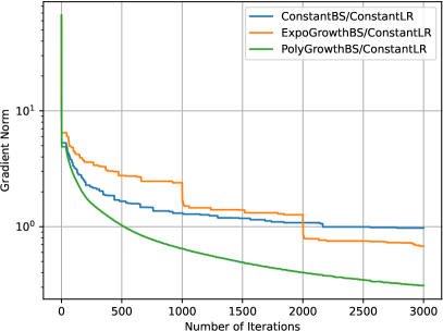
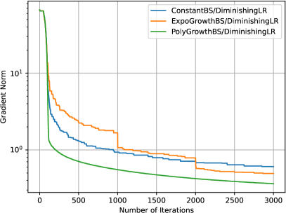
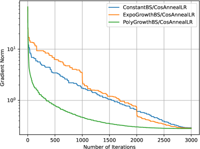
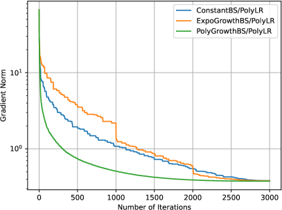
Figure 1: Norm of the gradient of the objective function against number of iterations for LRs (1), (2), (3), and (4) on COIL100 dataset.

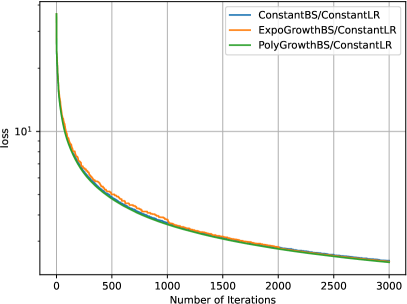
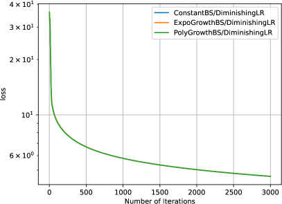
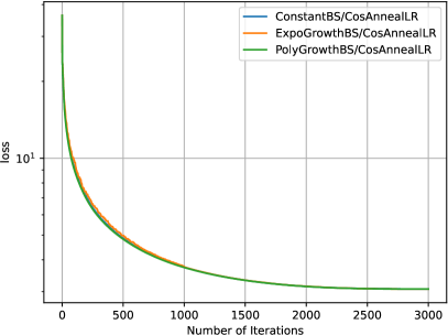
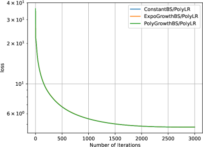
Figure 2: Objective function value against number of iterations for LRs (1), (2), (3), and (4) on COIL100 dataset.

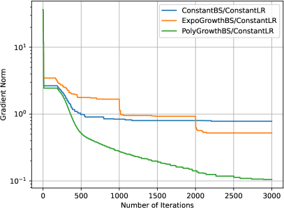
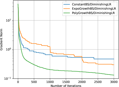
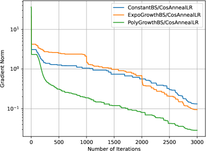
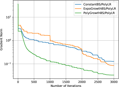
Figure 3: Norm of the gradient of the objective function against number of iterations for LRs (1), (2), (3), and (4) on MNIST dataset.

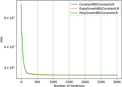
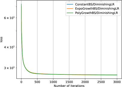
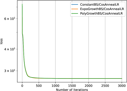
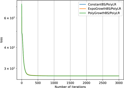
Figure 4: Objective function value against number of iterations for LRs (1), (2), (3), and (4) on MNIST dataset.

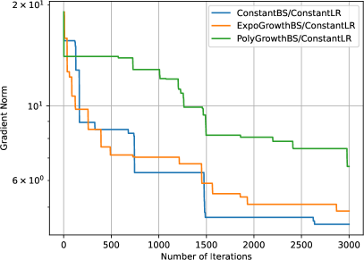
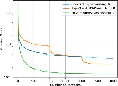
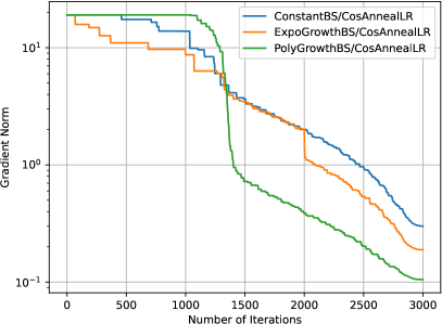
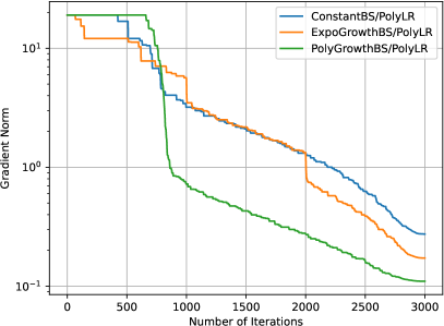
Figure 5: Norm of the gradient of the objective function against number of iterations for LRs (1), (2), (3), and (4) on MovieLens-1M dataset.

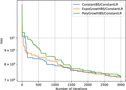
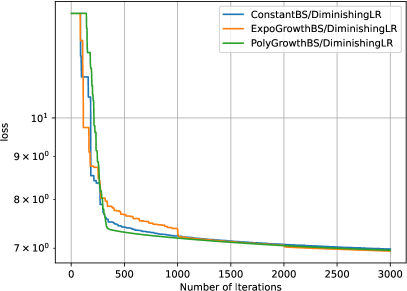
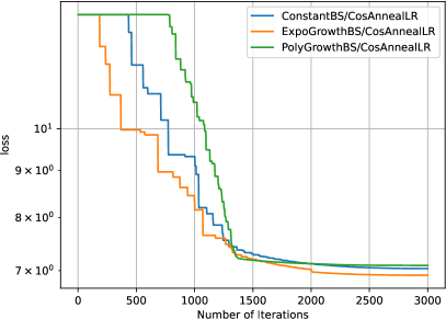
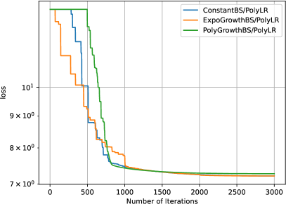
Figure 6: Objective function value against number of iterations for LRs (1), (2), (3), and (4) on MovieLens-1M dataset.

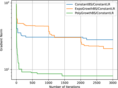
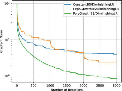
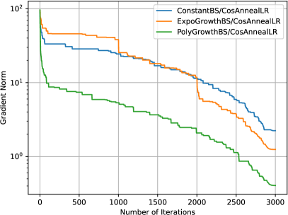
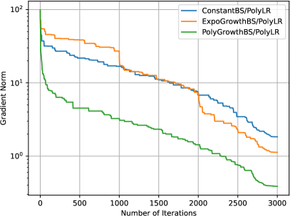
Figure 7: Norm of the gradient of the objective function against number of iterations for LRs (1), (2), (3), and (4) on Jester dataset.

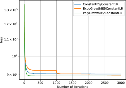
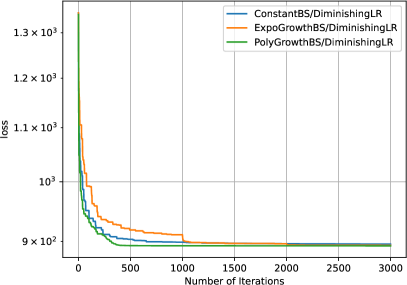
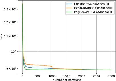
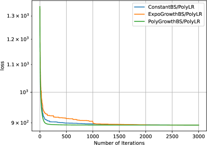
Figure 8: Objective function value against number of iterations for LRs (1), (2), (3), and (4) on Jester dataset.

We experimentally evaluated the performance of RSGD for the two types of BSs and various types of LRs introduced in Section 4. The experiments were based on those of Kasai et al. (2019) and Sakai & Iiduka (2025). They were run on an iMac (Intel Core i5, 2017) running the macOS Venture operating system (ver. 13.7.1). The algorithms were written in Python (3.12.7) using the NumPy (1.26.0) and Matplotlib (3.9.1) packages in accordance with the work of Sakai & Iiduka (2025). The Python codes are available https://anonymous.4open.science/r/202501-fastrsgd-DD56.

We set $p=2.0$ in (4) and $\eta_{\min}:=0$. In Cases (i) and (ii), we used an initial LR $\eta_{\max}$ selected from $\{0.5,0.1,0.05,0.01,0.005\}$. In Case (ii), we set $K=1000,\gamma=3.0$ and $a=c=2.0$. The details for Cases (iii) and (iv) are given in Appendix B.

5.1 Principal Component Analysis

We can formulate the principal component analysis (PCA) problem as an optimization problem on the Stiefel manifold (Kasai et al., 2019; Breloy et al., 2021); for a given dataset $\{x_{j}\}_{j=1,\ldots,N}\subset\mathbb{R}^{n}$ and $r$ $(\leq n)$,

minimize $$f(U)\coloneq\frac{1}{N}\sum_{j=1}^{N}\|x_{j}-UU^{\top}x_{j}\|^{2},$$

subject to $$U\in\mathrm{St}(r,n).$$

We set $r=10$ and used the COIL100 (Nene et al., 1996) and MNIST (LeCun et al., 1998) datasets. The Columbia Object Image Library (COIL100) dataset contains $7200$ color camera images of $100$ objects ($72$ poses per object) taken from different angles. As in previous work (Kasai et al., 2019; Sakai & Iiduka, 2025), we resized the images to $32\times 32$ pixels and transformed each one into a $1024(=32^{2})$ dimensional vector. Hence, we set $(N,n,r)=(7200,1024,10)$. The MNIST dataset contains $60,000$ $28\times 28$-pixel gray-scale images of handwritten numbers $0$ to $9$. As in previous work (Sakai & Iiduka, 2025), we transformed each image into a $784(=28^{2})$ dimensional vector and normalized each pixel to the range $[0,1]$. Hence, we set $(N,n,r)=(60000,784,10)$. Furthermore, we used a constant BS with $b_{t}\coloneq 2^{10}$ and an increasing BS with an initial value $b_{0}\coloneq 3^{5}$.

5.2 Low-rank Matrix Completion

The low-rank matrix completion (LRMC) problem involves completing an incomplete matrix $Z=(z_{1},\ldots,z_{N})\in\mathbb{R}^{n\times N}$; $\Omega$ denotes a set of indices for which we know the entries in $Z$. For $a\in\mathbb{R}^{n}$, we define $P_{\Omega_{i}}(a)$ such that the $j$-th element is $a_{j}$ if $(i,j)\in\Omega$ and $0$ otherwise. For $U\in\mathbb{R}^{n\times r},z\in\mathbb{R}^{n}$, $q_{j}(U,z):=\mathrm{argmin}_{a\in\mathbb{R}^{r}}\|P_{\Omega_{j}}(Ua-z)\|$. We can now formulate the LRMC problem as the following optimization problem on the Grassmann manifold (Boumal & Absil, 2015);

minimize $$f(U)\coloneq\frac{1}{N}\sum_{j=1}^{N}\|P_{\Omega_{j}}(Uq_{j}(U,z_{j})-z_{j})\|^{2},$$

subject to $$U\in\mathrm{Gr}(r,n).$$

We set $r=10$ and used the MovieLens-1M (Harper & Konstan, 2016) and Jester datasets (Goldberg et al., 2001). The MovieLens-1M dataset contains $1,000,209$ ratings given by $6040$ users on $3952$ movies. Every rating lies in $[0,5]$. As in previous work (Sakai & Iiduka, 2025), we normalized each rating to the range $[0,1]$. Hence, we set $(N,n,r)=(3952,6040,10)$. The Jester dataset contains ratings of $100$ jokes from $24,983$ users. Every rating lies in the range $[-10,10]$. Hence, we set $(N,n,r)=(24983,100,10)$. Furthermore, we used a constant BS with $b_{t}\coloneq 2^{8}$ and an increasing BS with an initial value $b_{0}\coloneq 3^{4}$.

The performance in terms of the gradient norm of the objective function against the number of iterations for LRs (1), (2), (3), and (4) on the COIL100, MNIST, MovieLens-1M, and Jester datasets are plotted in Figures 1, 3, 5, and 7, respectively. The performance in terms of the objective function value against the number of iterations for LRs (1), (2), (3), and (4) on the COIL100, MNIST, MovieLens-1M, and Jester datasets are shown in Figures 2, 4, 6, and 8, respectively. For the PCA problem, performance in terms of the gradient norm was better with an increasing BS than with a constant BS. However, the differences in the objective function values are small. One possible reason is that the objective function may be flat around the optimal solution. For the LRMC problem, performance in terms of the gradient norm was better with an increasing BS than with a constant BS, except for a constant BS and a constant LR on the MovieLens-1M dataset. Furthermore, performance in terms of the objective function value tended to be good with an increasing BS.

6 Conclusion and Future Direction

Our theoretical analysis using several learning rates, including cosine annealing and polynomial decay, demonstrated that using an increasing batch size rather than a constant batch size improves the convergence rate, and the results of our experiments support our theoretical results.

However, we did not analyze the use of adaptive methods such as RAdam and RAMSGrad (Bécigneul & Ganea, 2019; Kasai et al., 2019). In the Euclidean case, adaptive methods are empirically known to exhibit high performance on various tasks, including natural language processing. Therefore, applying our analysis to such algorithms would be an interesting and important direction for future work. Such extensions should improve convergence rates.

Appendix A Proof of The Propositions

A.1 Proof of Lemma 3.1

Proof.

Considering Assumption 2.2, we start with

$$f(x_{t+1}) \leq f(x_{t})-\eta_{t}\langle\mathrm{grad}f(x_{t}),\mathrm{grad}f_{B_{t}}(x_{t})\rangle_{x_{t}}+\frac{\eta_{t}^{2}}{2}L_{r}\|\mathrm{grad}f_{B_{t}}(x_{t})\|_{x_{t}}^{2},$$

$$\mathbb{E}[\|\mathrm{grad}f_{B_{t}}(x_{t})\|_{x_{t}}^{2}|\mathcal{F}_{t+1}] =\mathbb{E}[\|\mathrm{grad}f_{B_{t}}(x_{t})-\mathrm{grad}f(x_{t})+\mathrm{grad}f(x_{t})\|_{x_{t}}^{2}|\mathcal{F}_{t+1}]$$

$$\leq\mathbb{E}[\|\mathrm{grad}f_{B_{t}}(x_{t})-\mathrm{grad}f(x_{t})\|_{x_{t}}^{2}|\mathcal{F}_{t+1}]+\mathbb{E}[\|\mathrm{grad}f(x_{t})\|_{x_{t}}^{2}|\mathcal{F}_{t+1}]$$

$$\quad+2\mathbb{E}[\langle\mathrm{grad}f_{B_{t}}(x_{t})-\mathrm{grad}f(x_{t}),\mathrm{grad}f(x_{t})\rangle_{x_{t}}|\mathcal{F}_{t+1}]$$

$$=\mathbb{E}[\|\mathrm{grad}f_{B_{t}}(x_{t})-\mathrm{grad}f(x_{t})\|_{x_{t}}^{2}|\mathcal{F}_{t+1}]+\mathbb{E}[\|\mathrm{grad}f(x_{t})\|_{x_{t}}^{2}|\mathcal{F}_{t+1}]$$

$$\quad+2\langle\mathbb{E}[\mathrm{grad}f_{B_{t}}(x_{t})|\mathcal{F}_{t+1}]-\mathrm{grad}f(x_{t}),\mathrm{grad}f(x_{t})\rangle_{x_{t}}$$

$$\leq\frac{\sigma^{2}}{b_{t}}+\mathbb{E}[\|\mathrm{grad}f(x_{t})\|_{x_{t}}^{2}|\mathcal{F}_{t+1}]\qquad\text{a.s.},$$

and

$$\mathbb{E}[\langle\mathrm{grad}f(x_{t}),\mathrm{grad}f_{B_{t}}(x_{t})\rangle_{x_{t}}|\mathcal{F}_{t+1}]=\langle\mathrm{grad}f(x_{t}),\mathbb{E}[\mathrm{grad}f_{B_{t}}(x_{t})|\mathcal{F}_{t+1}]\rangle_{x_{t}}=\|\mathrm{grad}f(x_{t})\|_{x_{t}}^{2}\qquad\text{a.s.}$$

Taking the total expectation for the above equations, we have

$$\mathbb{E}[f(x_{t+1})] \leq\mathbb{E}[f(x_{t})]-\eta_{t}\mathbb{E}[\langle\mathrm{grad}f(x_{t}),\mathrm{grad}f_{B_{t}}(x_{t})\rangle_{x_{t}}]+\frac{\eta_{t}^{2}}{2}L_{r}\mathbb{E}[\|\mathrm{grad}f_{B_{t}}(x_{t})\|_{x_{t}}^{2}]$$

$$=\mathbb{E}[f(x_{t})]-\eta_{t}\mathbb{E}[\mathbb{E}[\langle\mathrm{grad}f(x_{t}),\mathrm{grad}f_{B_{t}}(x_{t})\rangle_{x_{t}}|\mathcal{F}_{t+1}]]+\frac{\eta_{t}^{2}}{2}L_{r}\mathbb{E}[\mathbb{E}[\|\mathrm{grad}f_{B_{t}}(x_{t})\|_{x_{t}}^{2}|\mathcal{F}_{t+1}]]$$

$$\leq\mathbb{E}[f(x_{t})]-\eta_{t}\mathbb{E}[\|\mathrm{grad}f(x_{t})\|_{x_{t}}^{2}]+\frac{\eta_{t}^{2}L_{r}}{2}\left(\frac{\sigma^{2}}{b_{t}}+\mathbb{E}[\|\mathrm{grad}f(x_{t})\|_{x_{t}}^{2}]\right)$$

$$=\mathbb{E}[f(x_{t})]+\frac{L_{r}\sigma^{2}\eta_{t}^{2}}{2b_{t}}-\eta_{t}\left(1-\frac{L_{r}\eta_{t}}{2}\right)\mathbb{E}[\|\mathrm{grad}f(x_{t})\|_{x_{t}}^{2}].$$

∎

A.2 Proof of Lemma 3.2

Proof.

Taking $\eta_{\max}<\frac{2}{L_{r}}$ into consideration, we start with

$$\sum_{t=0}^{T-1}\eta_{t}\left(1-\frac{L_{r}\eta_{t}}{2}\right)\mathbb{E}[\|\mathrm{grad}f(x_{t})\|_{x_{t}}^{2}]\geq\left(1-\frac{L_{r}\eta_{\max}}{2}\right)\min_{t\in\{0,\cdots,T-1\}}\mathbb{E}[\|\mathrm{grad}f(x_{t})\|_{x_{t}}^{2}]\sum_{t=0}^{T-1}\eta_{t}.$$

By taking the summation on both sides of the inequality for Lemma 3.1 and evaluating it using the above inequality, we obtain

$$\left(1-\frac{L_{r}\eta_{\max}}{2}\right)\min_{t\in\{0,\cdots,T-1\}}\mathbb{E}[\|\mathrm{grad}f(x_{t})\|_{x_{t}}^{2}]\sum_{t=0}^{T-1}\eta_{t}$$

$$\quad\leq\sum_{t=0}^{T-1}\eta_{t}\left(1-\frac{L_{r}\eta_{t}}{2}\right)\mathbb{E}[\|\mathrm{grad}f(x_{t})\|_{x_{t}}^{2}]$$

$$\quad\leq\sum_{t=0}^{T-1}(\mathbb{E}[f(x_{t})]-\mathbb{E}[f(x_{t+1})])+\sum_{t=0}^{T-1}\frac{L_{r}\sigma^{2}\eta_{t}^{2}}{2b_{t}}=\mathbb{E}[f(x_{0})-f(x_{T})]+\sum_{t=0}^{T-1}\frac{L_{r}\sigma^{2}\eta_{t}^{2}}{2b_{t}}.$$

$(\mathbb{E}[f(x_{t})])_{t\in\{0,\cdots,T\}}$ being a decreasing sequence implies

$$\mathbb{E}[f(x_{0})-f(x_{T})]\leq\mathbb{E}[f(x_{0})-f^{\star}]=f(x_{0})-f^{\star}.$$

Therefore,

$$\min_{t\in\{0,\cdots,T-1\}}\mathbb{E}[\|\mathrm{grad}f(x_{t})\|_{x_{t}}^{2}] \leq\frac{2(f(x_{0})-f^{\star})}{2-L_{r}\eta_{\max}}\frac{1}{\sum_{t=0}^{T-1}\eta_{t}}+\frac{L_{r}\sigma^{2}}{2-L_{r}\eta_{\max}}\frac{1}{\sum_{t=0}^{T-1}\eta_{t}}\sum_{t=0}^{T-1}\frac{\eta_{t}^{2}}{b_{t}}.$$

∎

A.3 Proof of Theorem 4.1

Proof.

We set $b_{t}=b$ in Lemma 3.2.
[Constant LR (1)]
From Lemma 3.2, we have

$$\sum_{t=0}^{T-1}\eta_{t}=\sum_{t=0}^{T-1}\eta_{\max}=\eta_{\max}T$$

and

$$\sum_{t=0}^{T-1}\frac{\eta_{t}^{2}}{b_{t}}=\frac{1}{\sum_{t=0}^{T-1}\eta_{\max}}\sum_{t=0}^{T-1}\frac{\eta_{\max}^{2}}{b}=\frac{\eta_{\max}^{2}}{b}T,$$

which imply

$$\min_{t\in\{0,\cdots,T-1\}}\mathbb{E}[\|\mathrm{grad}f(x_{t})\|_{x_{t}}^{2}]\leq\frac{2(f(x_{0})-f^{\star})}{(2-L_{r}\eta_{\max})\eta_{\max}T}+\frac{L_{r}\eta_{\max}}{2-L_{r}\eta_{\max}}\frac{\sigma^{2}}{b}.$$

[Diminishing LR (2)]
From Lemma 3.2, we have

$$\sum_{t=0}^{T-1}\eta_{t}=\eta_{\max}\sum_{t=0}^{T-1}\frac{1}{\sqrt{t+1}}\geq\eta_{\max}\sum_{t=0}^{T-1}\frac{1}{\sqrt{T}}=\eta_{\max}\frac{T}{\sqrt{T}}=\eta_{\max}\sqrt{T}$$

and

$$\sum_{t=0}^{T-1}\frac{\eta_{t}^{2}}{b_{t}}=\frac{\eta_{\max}^{2}}{b}\sum_{t=0}^{T-1}\frac{1}{t+1}\leq\frac{\eta_{\max}^{2}}{b}\left(1+\int_{1}^{T}\frac{dt}{t}\right)=\frac{\eta_{\max}^{2}}{b}+\frac{\eta_{\max}^{2}}{b}\log T,$$

which imply

$$\min_{t\in\{0,\cdots,T-1\}}\mathbb{E}[\|\mathrm{grad}f(x_{t})\|_{x_{t}}^{2}] \leq\frac{f(x_{0})-f^{\star}}{(2-L_{r}\eta_{\max})\eta_{\max}}\frac{1}{\sqrt{T}}+\frac{L_{r}\eta_{\max}}{2-L_{r}\eta_{\max}}\frac{\sigma^{2}}{b}\frac{1+\log T}{\sqrt{T}}.$$

[Cosine Annealing LR (3)]
From Lemma 3.2, we have

$$\sum_{t=0}^{T-1}\eta_{t} \geq\int_{0}^{T}\eta_{t}dt=\frac{\eta_{\max}+\eta_{\min}}{2}T+\frac{\eta_{\max}-\eta_{\min}}{2}\int_{0}^{T}\cos\left(\frac{t}{T}\pi\right)dt$$

$$=\frac{\eta_{\max}+\eta_{\min}}{2}T$$

and

$$\sum_{t=0}^{T-1}\eta_{t}^{2} =\frac{(\eta_{\max}+\eta_{\min})^{2}}{4}T+\frac{\eta_{\max}^{2}+\eta_{\min}^{2}}{2}\sum_{t=0}^{T-1}\cos\frac{t}{T}\pi+\frac{(\eta_{\max}-\eta_{\min})^{2}}{4}\sum_{t=0}^{T-1}\cos^{2}\frac{t}{T}\pi$$

$$\leq\frac{(\eta_{\max}+\eta_{\min})^{2}}{4}T+\frac{\eta_{\max}^{2}-\eta_{\min}^{2}}{2}T+\frac{(\eta_{\max}-\eta_{\min})^{2}}{4}T$$

$$=\eta_{\max}^{2}T,$$

which imply

$$\min_{t\in\{0,\cdots,T-1\}}\mathbb{E}[\|\mathrm{grad}f(x_{t})\|_{x_{t}}^{2}] \leq\frac{4(f(x_{0})-f^{\star})}{(2-L_{r}\eta_{\max})(\eta_{\max}+\eta_{\min})}\frac{1}{T}+\frac{2L_{r}\eta_{\max}^{2}}{(2-L_{r}\eta_{\max})(\eta_{\max}+\eta_{\min})}\frac{\sigma^{2}}{b}.$$

[Polynomial Decay LR (4)]
We start by recalling the Riemann integral (e.g., Rudin (1976)) of $g(t)\coloneq(1-t)^{p}\geq 0(0\leq t\leq 1)$. $U(P_{T})\coloneq\sum_{t=0}^{T-1}\frac{1}{T}(1-\frac{t}{T})^{p}$ is an upper Riemann sum with the function $g$ and a partition $P_{T}\coloneq\{0,\frac{1}{T},\cdots,\frac{T-1}{T},1\}$ due to $g$ being monotone decreasing. From the definition of an Riemann integral (e.g., Rudin (1976, Section 6)), if $\int_{0}^{1}g(t)dt$ exists, then

$$\inf_{P:\text{Partitions of [0,1]}}U(P)=\int_{0}^{1}g(t)dt.$$

In fact, the integral value exists. Thus, we obtain

$$\sum_{t=0}^{T-1}\frac{1}{T}\left(1-\frac{t}{T}\right)^{p}=U(P_{T})\geq\inf_{P:\text{Partitions of [0,1]}}U(P)=\int_{0}^{1}(1-t)^{p}dt=\frac{1}{p+1}.$$

Similarly, if we define $L(P_{T})$ as $\sum_{t=1}^{T}\frac{1}{T}\left(1-\frac{t}{T}\right)^{p}$, then $L(P_{T})$ is a lower Riemann sum with the function $g$ and a partition $P_{T}$, and the supremum of $L(P_{T})$ equals $\int_{0}^{1}g(t)dt$. Considering

$$\sum_{t=0}^{T-1}\frac{1}{T}\left(1-\frac{t}{T}\right)^{p}=L(P_{T})+\frac{1}{T},$$

we have

$$\sum_{t=0}^{T-1}\frac{1}{T}\left(1-\frac{t}{T}\right)^{p}=L(P_{T})+\frac{1}{T}\leq\sup_{P:\text{Partitions of [0,1]}}L(P)+\frac{1}{T}=\int_{0}^{1}(1-t)^{p}dt+\frac{1}{T}=\frac{1}{p+1}+\frac{1}{T}.$$

Hence,

$$\frac{T}{p+1}\leq\sum_{t=0}^{T-1}\left(1-\frac{t}{T}\right)^{p}\leq\frac{T}{p+1}+1$$

holds. By replacing $g$ with $(1+t)^{2p}(0\leq t\leq 1)$ and using the same logic, we obtain

$$\sum_{t=0}^{T-1}\frac{1}{T}\left(1-\frac{t}{T}\right)^{2p}\leq\int_{0}^{1}(1-t)^{2p}dt+\frac{1}{T}=\frac{1}{2p+1}+\frac{1}{T}.$$

Therefore, considering Lemma 3.2,

$$\sum_{t=0}^{T-1}\eta_{t} =\eta_{\min}T+(\eta_{\max}-\eta_{\min})\sum_{t=0}^{T-1}\left(1-\frac{t}{T}\right)^{p}$$

$$\geq\eta_{\min}T+(\eta_{\max}-\eta_{\min})\frac{T}{p+1}=\frac{\eta_{\max}+p\eta_{\min}}{p+1}T,$$

and

$$\sum_{t=0}^{T-1}\eta_{t}^{2} =\eta_{\min}T+2\eta_{\min}(\eta_{\max}-\eta_{\min})\sum_{t=0}^{T-1}\left(1-\frac{t}{T}\right)^{p}+(\eta_{\max}-\eta_{\min})^{2}\sum_{t=0}^{T-1}\left(1-\frac{t}{T}\right)^{2p}$$

$$\leq\eta_{\min}T+2\eta_{\min}(\eta_{\max}-\eta_{\min})\left(1+\frac{T}{p+1}\right)+(\eta_{\max}-\eta_{\min})^{2}\left(1+\frac{T}{2p+1}\right)$$

$$=\eta_{\max}^{2}-\eta_{\min}^{2}+\left(\eta_{\min}+\frac{2\eta_{\min}(\eta_{\max}-\eta_{\min})}{p+1}+\frac{(\eta_{\max}-\eta_{\min})^{2}}{2p+1}\right)T,$$

we have

$$\min_{t\in\{0,\cdots,T-1\}}\mathbb{E}[\|\mathrm{grad}f(x_{t})\|_{x_{t}}^{2}]$$

$$\leq\frac{p+1}{(2-L_{r}\eta_{\max})(\eta_{\max}+p\eta_{\min})}\left\{2(f(x_{0})-f^{\star})+\frac{L_{r}(\eta_{\max}^{2}-\eta_{\min}^{2})\sigma^{2}}{b}\right\}\frac{1}{T}$$

$$\quad+\frac{L_{r}(p+1)(\eta_{\max}^{2}-\eta_{\min}^{2})}{(2-L_{r}\eta_{\max})(\eta_{\max}+p\eta_{\min})}\left(\eta_{\min}+\frac{2\eta_{\min}(\eta_{\max}-\eta_{\min})}{p+1}+\frac{(\eta_{\max}-\eta_{\min})^{2}}{2p+1}\right)\frac{\sigma^{2}}{b}.$$

∎

A.4 Proof of Theorem 4.2

Proof.

The evaluations in all these cases are based on Lemma 3.2 and use estimations of $\sum_{t=0}^{T-1}\eta_{t}$ in the proof of Theorem 4.1.
[Exponential Growth BS (5) and Constant LR (1)]
From the fact that sums of positive term series are the supremum of their finite sums, we have

$$\sum_{t=0}^{T-1}\frac{1}{b_{t}}=\sum_{m=0}^{M-1}\frac{K}{b_{0}\gamma^{m}}+\frac{T-KM}{b_{0}\gamma^{M}}\leq\sum_{m=0}^{M}\frac{K}{b_{0}\gamma^{m}}\leq\frac{K}{b_{0}}\sum_{m=0}^{\infty}\frac{1}{\gamma^{m}}=\frac{K\gamma}{b_{0}(\gamma-1)},$$ (9)

which implies

$$\sum_{t=0}^{T-1}\frac{\eta_{\max}^{2}}{b_{t}}=\eta_{\max}^{2}\sum_{t=0}^{T-1}\frac{1}{b_{t}}\leq\frac{\eta_{\max}^{2}K\gamma}{b_{0}(\gamma-1)}.$$

Therefore,

$$\min_{t\in\{0,\cdots,T-1\}}\mathbb{E}[\|\mathrm{grad}f(x_{t})\|_{x_{t}}^{2}]\leq\frac{1}{(2-L_{r}\eta_{\max})\eta_{\max}}\left\{2(f(x_{0})-f^{\star})+\frac{L_{r}\eta_{\max}^{2}K\gamma}{\gamma-1}\frac{\sigma^{2}}{b_{0}}\right\}\frac{1}{T}.$$

[Exponential Growth BS (5) and Diminishing LR (2)]
Using (9), we have

$$\sum_{t=0}^{T-1}\frac{\eta_{t}^{2}}{b_{t}}=\eta_{\max}^{2}\sum_{t=0}^{T-1}\frac{1}{(t+1)b_{t}}\leq\eta_{\max}^{2}\sum_{t=0}^{T-1}\frac{1}{b_{t}}\leq\frac{\eta_{\max}^{2}K\gamma}{b_{0}(\gamma-1)},$$

which implies

$$\min_{t\in\{0,\cdots,T-1\}}\mathbb{E}[\|\mathrm{grad}f(x_{t})\|_{x_{t}}^{2}]\leq\frac{1}{(2-L_{r}\eta_{\max})\eta_{\max}}\left\{2(f(x_{0})-f^{\star})+\frac{L_{r}\eta_{\max}^{2}K\gamma}{\gamma-1}\frac{\sigma^{2}}{b_{0}}\right\}\frac{1}{\sqrt{T}}.$$

[Exponential Growth BS (5) and Cosine Annealing LR (3)]
From (9) and $|\cos x|\leq 1$, we have

$$\sum_{t=0}^{T-1}\frac{\eta_{t}^{2}}{b_{t}} =\sum_{t=0}^{T-1}\frac{1}{b_{t}}\left(\frac{(\eta_{\max}+\eta_{\min})^{2}}{4}+\frac{(\eta_{\max}-\eta_{\min})^{2}}{4}\cos^{2}\frac{t}{T}\pi+\frac{\eta_{\max}^{2}-\eta_{\min}^{2}}{2}\cos\frac{t}{T}\pi\right)$$

$$\leq\eta_{\max}^{2}\sum_{t=0}^{T-1}\frac{1}{b_{t}}\leq\frac{\eta_{\max}^{2}K\gamma}{b_{0}(\gamma-1)},$$

which implies

$$\min_{t\in\{0,\cdots,T-1\}}\mathbb{E}[\|\mathrm{grad}f(x_{t})\|_{x_{t}}^{2}]\leq\frac{2}{(2-L_{r}\eta_{\max})(\eta_{\max}+\eta_{\min})}\left\{2(f(x_{0})-f^{\star})+\frac{L_{r}\eta_{\max}^{2}K\gamma}{\gamma-1}\frac{\sigma^{2}}{b_{0}}\right\}\frac{1}{T}.$$

[Exponential Growth BS (5) and Polynomial Decay LR (4)]
From (9) and $t\leq T$, we have

$$\sum_{t=0}^{T-1}\frac{\eta_{t}^{2}}{b_{t}} =\sum_{t=0}^{T-1}\frac{1}{b_{t}}\left\{\eta_{\min}^{2}+(\eta_{\max}-\eta_{\min})^{2}\left(1-\frac{t}{T}\right)^{2p}+2\eta_{\min}(\eta_{\max}-\eta_{\min})\left(1-\frac{t}{T}\right)^{p}\right\}$$

$$\leq\eta_{\max}^{2}\sum_{t=0}^{T-1}\frac{1}{b_{t}}\leq\frac{\eta_{\max}^{2}K\gamma}{b_{0}(\gamma-1)},$$

which implies

$$\min_{t\in\{0,\cdots,T-1\}}\mathbb{E}[\|\mathrm{grad}f(x_{t})\|_{x_{t}}^{2}] \leq\frac{p+1}{(2-L_{r}\eta_{\max})(\eta_{\max}+p\eta_{\min})}\left\{2(f(x_{0})-f^{\star})+\frac{L_{r}\eta_{\max}^{2}K\gamma}{\gamma-1}\frac{\sigma^{2}}{b_{0}}\right\}\frac{1}{T}.$$

[Polynomial Growth BS (6) and Constant LR (1)]
We set $\underline{a}\coloneq a\land b_{0}$. Considering $c>1$, we have

$$\sum_{t=0}^{T-1}\frac{1}{b_{t}} =\sum_{m=0}^{M-1}\frac{K}{(am+b_{0})^{c}}+\frac{T-KM}{(aM+b_{0})^{c}}\leq\sum_{m=0}^{M}\frac{K}{(am+b_{0})^{c}}\leq\frac{K}{\underline{a}^{\lfloor c\rfloor}}\sum_{m=0}^{M}\frac{1}{(m+1)^{c}}$$

$$=\frac{K}{\underline{a}^{\lfloor c\rfloor}}\sum_{m=1}^{\infty}\frac{1}{m^{c}}=\frac{K\zeta(c)}{\underline{a}^{\lfloor c\rfloor}},$$ (10)

which implies

$$\sum_{t=0}^{T-1}\frac{\eta_{t}^{2}}{b_{t}}=\eta_{\max}^{2}\sum_{t=0}^{T-1}\frac{1}{b_{t}}\leq\frac{\eta_{\max}^{2}K\zeta(c)}{\underline{a}^{\lfloor c\rfloor}}.$$

Therefore,

$$\min_{t\in\{0,\cdots,T-1\}}\mathbb{E}[\|\mathrm{grad}f(x_{t})\|_{x_{t}}^{2}]\leq\frac{1}{(2-L_{r}\eta_{\max})\eta_{\max}}\left(2(f(x_{0})-f^{\star})+\frac{L_{r}\eta_{\max}^{2}K\zeta(c)\sigma^{2}}{\underline{a}^{\lfloor c\rfloor}}\right)\frac{1}{T},$$

where, for $c>1$, Riemann zeta function $\zeta(c)<\infty$; $\zeta(c)$ is monotone decreasing on $c\in(1,\infty)$ and $\underset{c\to\infty}{\lim}\zeta(c)=1$.

[Polynomial Growth BS (6) and Diminishing LR (2)]
From (A.4), we have

$$\sum_{t=0}^{T-1}\frac{\eta_{t}^{2}}{b_{t}}=\eta_{\max}^{2}\sum_{t=0}^{T-1}\frac{1}{(t+1)b_{t}}\leq\eta_{\max}^{2}\sum_{t=0}^{T-1}\frac{1}{b_{t}}\leq\frac{\eta_{\max}^{2}K\zeta(c)}{\underline{a}^{\lfloor c\rfloor}},$$

which implies

$$\min_{t\in\{0,\cdots,T-1\}}\mathbb{E}[\|\mathrm{grad}f(x_{t})\|_{x_{t}}^{2}]\leq\frac{1}{(2-L_{r}\eta_{\max})\eta_{\max}}\left(2(f(x_{0})-f^{\star})+\frac{L_{r}\eta_{\max}^{2}K\zeta(c)\sigma^{2}}{\underline{a}^{\lfloor c\rfloor}}\right)\frac{1}{\sqrt{T}}.$$

[Polynomial Growth BS (6) and Cosine Annealing LR (3)]
From (A.4) and the previous analysis for Cosine Annealing LR (3), we have

$$\sum_{t=0}^{T-1}\frac{\eta_{t}^{2}}{b_{t}}\leq\eta_{\max}^{2}\sum_{t=0}^{T-1}\frac{1}{b_{t}}\leq\frac{\eta_{\max}^{2}K\zeta(c)}{\underline{a}^{\lfloor c\rfloor}},$$

which implies

$$\min_{t\in\{0,\cdots,T-1\}}\mathbb{E}[\|\mathrm{grad}f(x_{t})\|_{x_{t}}^{2}]\quad\leq\frac{2}{(2-L_{r}\eta_{\max})(\eta_{\max}+\eta_{\min})}\left(2(f(x_{0})-f^{\star})+\frac{L_{r}\eta_{\max}^{2}K\zeta(c)\sigma^{2}}{\underline{a}^{\lfloor c\rfloor}}\right)\frac{1}{T}.$$

[Polynomial Growth BS (6) and Polynomial Decay LR (4)]
From (A.4) and the previous analysis for Polynomial Decay LR (4), we have

$$\sum_{t=0}^{T-1}\frac{\eta_{t}^{2}}{b_{t}}\leq\eta_{\max}^{2}\sum_{t=0}^{T-1}\frac{1}{b_{t}}\leq\frac{\eta_{\max}^{2}K\zeta(c)}{\underline{a}^{\lfloor c\rfloor}},$$

which implies

$$\min_{t\in\{0,\cdots,T-1\}}\mathbb{E}[\|\mathrm{grad}f(x_{t})\|_{x_{t}}^{2}]\quad\leq\frac{p+1}{(2-L_{r}\eta_{\max})(\eta_{\max}+p\eta_{\min})}\left(2(f(x_{0})-f^{\star})+\frac{L_{r}\eta_{\max}^{2}K\zeta(c)\sigma^{2}}{\underline{a}^{\lfloor c\rfloor}}\right)\frac{1}{T}.$$

∎

A.5 Proof of Theorem 4.3

Proof.

The evaluations in all these cases are based on Lemma 3.2. We start with an exponential growth BS and a warm-up LR. From $l,l_{w}\in\mathbb{N}$ and $l_{w}\geq l$, there exist $\alpha,\beta\in\mathbb{N}\cup\{0\}$ such that $l_{w}=\alpha l+\beta$. Note that we define summations from $0$ to $-1$ as $0$. Furthermore, from $\forall u,v>0:0\leq u^{2}+v^{2}+uv$ holds.
[LR Decay Part: Constant (1)]
Considering $T_{w}=l_{w}K^{\prime}=\alpha(lK^{\prime})+\beta K^{\prime}$, we have

$$\sum_{t=T_{w}}^{T-1}\eta_{t} =\sum_{t=T_{w}}^{T-1}\eta_{\max}=(T-T_{w})\eta_{\max}$$

and

$$\sum_{t=T_{w}}^{T-1}\frac{\eta_{t}^{2}}{b_{t}}=\sum_{t=l_{w}K^{\prime}}^{(\alpha+1)l-1}\frac{\eta_{\max}^{2}}{b_{t}}+\sum_{t=(\alpha+1)l}^{T-1}\frac{\eta_{\max}^{2}}{b_{t}}=\sum_{t=T_{w}}^{T-1}\frac{\eta_{\max}^{2}}{b_{t}}\leq\frac{\eta_{\max}^{2}K}{b_{0}}\sum_{m=0}^{M}\frac{1}{\gamma^{m}}\leq\frac{\eta_{\max}^{2}K}{b_{0}}\sum_{m=0}^{\infty}\frac{1}{\gamma^{m}}=\frac{\eta_{\max}^{2}\gamma K}{(\gamma-1)b_{0}},$$

which imply

$$\min_{t\in\{T_{w},\cdots,T-1\}}\mathbb{E}[\|\mathrm{grad}f(x_{t})\|_{x_{t}}^{2}]\leq\frac{1}{(2-L_{r}\eta_{\max})\eta_{\max}}\left(2(f(x_{0})-f^{\star})+\frac{L_{r}\eta_{\max}^{2}K\gamma}{\gamma-1}\frac{\sigma^{2}}{b_{0}}\right)\frac{1}{T-T_{w}}.$$

[LR Decay Part: Diminishing (2)]
Similarly, we have

$$\sum_{t=T_{w}}^{T-1}\eta_{t} =\sum_{t=T_{w}}^{T-1}\frac{\eta_{\max}}{\sqrt{t+1}}\geq\eta_{\max}\int_{T_{w}}^{T}\frac{dt}{\sqrt{t+1}}=2\eta_{\max}(\sqrt{T+1}-\sqrt{T_{w}+1})$$

and

$$\sum_{t=0}^{T-1}\frac{\eta_{t}^{2}}{b_{t}}\leq\sum_{t=T_{w}}^{T-1}\frac{\eta_{\max}^{2}}{b_{t}(t+1)}\leq\sum_{t=T_{w}}^{T-1}\frac{\eta_{\max}^{2}}{b_{t}}\leq\frac{\eta_{\max}^{2}\gamma K}{(\gamma-1)b_{0}},$$

which imply

$$\min_{t\in\{T_{w},\cdots,T-1\}}\mathbb{E}[\|\mathrm{grad}f(x_{t})\|_{x_{t}}^{2}]\leq\frac{1}{2(2-L_{r}\eta_{\max})\eta_{\max}}\left(2(f(x_{0})-f^{\star})+\frac{L_{r}\eta_{\max}^{2}K\gamma}{\gamma-1}\frac{\sigma^{2}}{b_{0}}\right)\frac{1}{\sqrt{T+1}-\sqrt{T_{w}+1}}.$$

[LR Decay Part: Cosine Annealing (3)]
We have

$$\sum_{t=T_{w}}^{T-1}\eta_{t} =\sum_{t=T_{w}}^{T-1}\left(\frac{\eta_{\max}+\eta_{\min}}{2}+\frac{\eta_{\max}-\eta_{\min}}{2}\cos\frac{t-T_{w}}{T-T_{w}}\pi\right)$$

$$=\frac{\eta_{\max}+\eta_{\min}}{2}(T-T_{w})+\frac{\eta_{\max}-\eta_{\min}}{2}\sum_{t=T_{w}}^{T-1}\cos\frac{t-T_{w}}{T-T_{w}}\pi$$

$$\geq\frac{\eta_{\max}+\eta_{\min}}{2}(T-T_{w})+\frac{\eta_{\max}-\eta_{\min}}{2}\int_{T_{w}}^{T}\cos\left(\frac{t-T_{w}}{T-T_{w}}\pi\right)dt=\frac{\eta_{\max}+\eta_{\min}}{2}(T-T_{w})$$

and

$$\sum_{t=T_{w}}^{T-1}\frac{\eta_{t}^{2}}{b_{t}} \leq\sum_{t=T_{w}}^{T-1}\frac{1}{b_{t}}\left(\frac{(\eta_{\max}+\eta_{\min})^{2}}{4}+\frac{\eta_{\max}^{2}-\eta_{\min}^{2}}{2}\cos\frac{t-T_{w}}{T-T_{w}}\pi+\frac{(\eta_{\max}-\eta_{\min})^{2}}{4}\cos^{2}\frac{t-T_{w}}{T-T_{w}}\pi\right)$$

$$\leq\sum_{t=0}^{T-1}\frac{1}{b_{t}}\left(\frac{(\eta_{\max}+\eta_{\min})^{2}}{4}+\frac{\eta_{\max}^{2}-\eta_{\min}^{2}}{2}+\frac{(\eta_{\max}-\eta_{\min})^{2}}{4}\right)=\sum_{t=0}^{T-1}\frac{\eta_{\max}^{2}}{b_{t}}\leq\frac{\eta_{\max}^{2}\gamma K}{(\gamma-1)b_{0}},$$

which imply

$$\min_{t\in\{T_{w},\cdots,T-1\}}\mathbb{E}[\|\mathrm{grad}f(x_{t})\|_{x_{t}}^{2}]\leq\frac{2}{(2-L_{r}\eta_{\max})(\eta_{\max}+\eta_{\min})}\left(2(f(x_{0})-f^{\star})+\frac{L_{r}\eta_{\max}^{2}K\gamma}{\gamma-1}\frac{\sigma^{2}}{b_{0}}\right)\frac{1}{T-T_{w}}.$$

[LR Decay Part: Polynomial Decay (4)]
As with the proof of polynomial decay LR (4) in Theorem 4.1, we have

$$\sum_{t=T_{w}}^{T-1}\eta_{t} =\sum_{t=T_{w}}^{T-1}\left\{\eta_{\min}+(\eta_{\max}-\eta_{\min})\left(1-\frac{t-T_{w}}{T-T_{w}}\right)^{p}\right\}$$

$$\geq\eta_{\min}(T-T_{w})+(\eta_{\max}-\eta_{\min})\frac{T-T_{w}}{p+1}=\frac{\eta_{\max}+p\eta_{\min}}{p+1}(T-T_{w})$$

and

$$\sum_{t=T_{w}}^{T-1}\frac{\eta_{t}^{2}}{b_{t}} \leq\sum_{t=T_{w}}^{T-1}\frac{1}{b_{t}}\left(\eta_{\min}^{2}+(\eta_{\max}-\eta_{\min})^{2}\left(1-\frac{t-T_{w}}{T-T_{w}}\right)^{2p}+2\eta_{\min}(\eta_{\max}-\eta_{\min})\left(1-\frac{t-T_{w}}{T-T_{w}}\right)^{p}\right)$$

$$\leq\sum_{t=T_{w}}^{T-1}\frac{\eta_{\max}^{2}}{b_{t}}\leq\frac{\eta_{\max}^{2}\gamma K}{(\gamma-1)b_{0}},$$

which imply

$$\min_{t\in\{T_{w},\cdots,T-1\}}\mathbb{E}[\|\mathrm{grad}f(x_{t})\|_{x_{t}}^{2}]\leq\frac{p+1}{(2-L_{r}\eta_{\max})(\eta_{\max}+p\eta_{\min})}\left(2(f(x_{0})-f^{\star})+\frac{L_{r}\eta_{\max}^{2}K\gamma}{\gamma-1}\frac{\sigma^{2}}{b_{0}}\right)\frac{1}{T-T_{w}}.$$

On the other hand, we consider a polynomial growth BS and a warm-up LR.
[LR Decay Part: Constant (1)]
We have

$$\sum_{t=T_{w}}^{T-1}\eta_{t}=\sum_{t=T_{w}}^{T-1}\eta_{\max}=\eta_{\max}(T-T_{w})$$

and

$$\sum_{t=T_{w}}^{T-1}\frac{\eta_{t}^{2}}{b_{t}} =\sum_{t=l_{w}K^{\prime}}^{(\alpha+1)l-1}\frac{\eta_{\max}^{2}}{b_{t}}+\sum_{(\alpha+1)l}^{T-1}\frac{\eta_{\max}^{2}}{b_{t}}=\sum_{t=T_{w}}^{T-1}\frac{\eta_{\max}^{2}}{b_{t}}\leq\frac{\eta_{\max}^{2}K}{\underline{a}^{\lfloor c\rfloor}}\sum_{m=0}^{M-1}\frac{1}{(m+1)^{c}}\leq\frac{\eta_{\max}^{2}K}{\underline{a}^{\lfloor c\rfloor}}\sum_{m=1}^{\infty}\frac{1}{m^{c}}=\frac{\eta_{\max}^{2}K\zeta(c)}{\underline{a}^{\lfloor c\rfloor}},$$

which imply

$$\min_{t\in\{T_{w},\cdots,T-1\}}\mathbb{E}[\|\mathrm{grad}f(x_{t})\|_{x_{t}}^{2}]\leq\frac{1}{(2-L_{r}\eta_{\max})\eta_{\max}}\left(2(f(x_{0})-f^{\star})+\frac{L_{r}\eta_{\max}^{2}K\zeta(c)\sigma^{2}}{\underline{a}^{\lfloor c\rfloor}}\right)\frac{1}{T-T_{w}}.$$

[LR Decay Part: Diminishing (2)]
Similarly, we have

$$\sum_{t=T_{w}}^{T-1}\eta_{t}=\sum_{t=T_{w}}^{T-1}\frac{\eta_{\max}}{\sqrt{t+1}}\geq\eta_{\max}\int_{T_{w}}^{T}\frac{dt}{\sqrt{t+1}}=2\eta_{\max}(\sqrt{T+1}-\sqrt{T_{w}+1})$$

and

$$\sum_{t=T_{w}}^{T-1}\frac{\eta_{t}^{2}}{b_{t}}=\sum_{t=T_{w}}^{T-1}\frac{\eta_{\max}^{2}}{b_{t}(t+1)}\leq\sum_{t=T_{w}}^{T-1}\frac{\eta_{\max}^{2}}{b_{t}}\leq\frac{\eta_{\max}^{2}K\zeta(c)}{\underline{a}^{\lfloor c\rfloor}},$$

which imply

$$\min_{t\in\{T_{w},\cdots,T-1\}}\mathbb{E}[\|\mathrm{grad}f(x_{t})\|_{x_{t}}^{2}]\leq\frac{1}{2(2-L_{r}\eta_{\max})\eta_{\max}}\left(2(f(x_{0})-f^{\star})+\frac{L_{r}\eta_{\max}^{2}K\zeta(c)\sigma^{2}}{\underline{a}^{\lfloor c\rfloor}}\right)\frac{1}{\sqrt{T+1}-\sqrt{T_{w}+1}}.$$

[LR Decay Part: Cosine Annealing (3)]
We have

$$\sum_{t=T_{w}}^{T-1}\eta_{t} =\sum_{t=T_{w}}^{T-1}\left(\frac{\eta_{\max}+\eta_{\min}}{2}+\frac{\eta_{\max}-\eta_{\min}}{2}\cos\frac{t-T_{w}}{T-T_{w}}\pi\right)$$

$$\geq\frac{\eta_{\max}+\eta_{\min}}{2}(T-T_{w})+\frac{\eta_{\max}-\eta_{\min}}{2}\int_{T_{w}}^{T}\cos\left(\frac{t-T_{w}}{T-T_{w}}\pi\right)dt=\frac{\eta_{\max}+\eta_{\min}}{2}(T-T_{w})$$

and

$$\sum_{t=T_{w}}^{T-1}\frac{\eta_{t}^{2}}{b_{t}} =\sum_{t=T_{w}}^{T-1}\frac{1}{b_{t}}\left(\frac{(\eta_{\max}+\eta_{\min})^{2}}{4}+\frac{\eta_{\max}^{2}-\eta_{\min}^{2}}{2}\cos\frac{t-T_{w}}{T-T_{w}}\pi+\frac{(\eta_{\max}-\eta_{\min})^{2}}{4}\cos^{2}\frac{t-T_{w}}{T-T_{w}}\pi\right)$$

$$\leq\sum_{t=T_{w}}^{T-1}\frac{1}{b_{t}}\left(\frac{(\eta_{\max}+\eta_{\min})^{2}}{4}+\frac{\eta_{\max}^{2}-\eta_{\min}^{2}}{2}+\frac{(\eta_{\max}-\eta_{\min})^{2}}{4}\right)=\sum_{t=T_{w}}^{T-1}\frac{\eta_{\max}^{2}}{b_{t}}\leq\frac{\eta_{\max}^{2}K\zeta(c)}{\underline{a}^{\lfloor c\rfloor}},$$

which imply

$$\min_{t\in\{T_{w},\cdots,T-1\}}\mathbb{E}[\|\mathrm{grad}f(x_{t})\|_{x_{t}}^{2}]\leq\frac{2}{(2-L_{r}\eta_{\max})(\eta_{\max}+\eta_{\min})}\left(2(f(x_{0})-f^{\star})+\frac{L_{r}\eta_{\max}^{2}K\zeta(c)\sigma^{2}}{\underline{a}^{\lfloor c\rfloor}}\right)\frac{1}{T-T_{w}}.$$

[LR Decay Part: Polynomial Decay (4)]
Considering the proof of Polynomial Decay LR (4) in Theorem 4.1, we have

$$\sum_{t=T_{w}}^{T-1}\eta_{t} =\sum_{t=T_{w}}^{T-1}\left(\eta_{\min}+(\eta_{\max}-\eta_{\min})\left(1-\frac{t-T_{w}}{T-T_{w}}\right)^{p}\right)\geq\eta_{\min}(T-T_{w})+(\eta_{\max}-\eta_{\min})\frac{T-T_{w}}{p+1}$$

$$=\frac{\eta_{\max}+p\eta_{\min}}{p+1}(T-T_{w})$$

and

$$\sum_{t=T_{w}}^{T-1}\frac{\eta_{t}^{2}}{b_{t}} =\sum_{t=T_{w}}^{T-1}\frac{1}{b_{t}}\left(\eta_{\min}^{2}+(\eta_{\max}^{2}-\eta_{\min})^{2}\left(1-\frac{t-T_{w}}{T-T_{w}}\right)^{2p}+2\eta_{\min}(\eta_{\max}-\eta_{\min})\left(1-\frac{t-T_{w}}{T-T_{w}}\right)^{p}\right)$$

$$\leq\sum_{t=T_{w}}^{T-1}\frac{\eta_{\max}^{2}}{b_{t}}\leq\frac{\eta_{\max}^{2}K\zeta(c)}{\underline{a}^{\lfloor c\rfloor}},$$

which imply

$$\min_{t\in\{T_{w},\cdots,T-1\}}\mathbb{E}[\|\mathrm{grad}f(x_{t})\|_{x_{t}}^{2}]\leq\frac{p+1}{(2-L_{r}\eta_{\max})(\eta_{\max}+p\eta_{\min})}\left(2(f(x_{0})-f^{\star})+\frac{L_{r}\eta_{\max}^{2}K\zeta(c)\sigma^{2}}{\underline{a}^{\lfloor c\rfloor}}\right)\frac{1}{T-T_{w}}.$$

∎

A.6 Proof of Theorem 4.4

Proof.

[LR Decay Part: Constant (1)]
Considering A.5, we have

$$\sum_{t=T_{w}}^{T-1}\frac{\eta_{t}^{2}}{b_{t}}=\frac{\eta_{\max}^{2}}{b}(T-T_{w}),$$

which implies

$$\min_{t\in\{T_{w},\cdots,T-1\}}\mathbb{E}[\|\mathrm{grad}f(x_{t})\|_{x_{t}}^{2}]\leq\frac{2(f(x_{0})-f^{\star})}{(2-L_{r}\eta_{\max})\eta_{\max}}\frac{1}{T-T_{w}}+\frac{L_{r}\eta_{\max}}{2-L_{r}\eta_{\max}}\frac{\sigma^{2}}{b}.$$

[LR Decay Part: Diminishing (2)]
Similarly, we have

$$\sum_{t=T_{w}}^{T-1}\frac{\eta_{t}^{2}}{b_{t}}=\frac{\eta_{\max}^{2}}{b}\sum_{t=T_{w}}^{T-1}\frac{1}{t+1}\leq\frac{\eta_{\max}^{2}}{b}\left(1+\int_{T_{w}}^{T}\frac{dt}{t}\right)=\frac{\eta_{\max}^{2}}{b}+\frac{\eta_{\max}^{2}}{b}\log\frac{T}{T_{w}},$$

which implies

$$\min_{t\in\{T_{w},\cdots,T-1\}}\mathbb{E}[\|\mathrm{grad}f(x_{t})\|_{x_{t}}^{2}]\leq\frac{f(x_{0})-f^{\star}}{(2-L_{r}\eta_{\max})\eta_{\max}}\frac{1}{\sqrt{T+1}-\sqrt{T_{w}+1}}+\frac{L_{r}\eta_{\max}}{2(2-L_{r}\eta_{\max})}\frac{\sigma^{2}}{b}\frac{1+\log\frac{T}{T_{w}}}{\sqrt{T+1}-\sqrt{T_{w}+1}}.$$

[LR Decay Part: Cosine Annealing (3)]
Doing the same with A.5, we have

$$\sum_{t=T_{w}}^{T-1}\frac{\eta_{t}^{2}}{b_{t}} =\frac{1}{b}\sum_{t=T_{w}}^{T-1}\left(\frac{(\eta_{\max}+\eta_{\min})^{2}}{4}+\frac{\eta_{\max}^{2}-\eta_{\min}^{2}}{2}\cos\frac{t-T_{w}}{T-T_{w}}\pi+\frac{(\eta_{\max}-\eta_{\min})^{2}}{4}\cos^{2}\frac{t-T_{w}}{T-T_{w}}\pi\right)$$

$$\leq\frac{1}{b}\sum_{t=T_{w}}^{T-1}\left(\frac{(\eta_{\max}+\eta_{\min})^{2}}{4}+\frac{\eta_{\max}^{2}-\eta_{\min}^{2}}{2}+\frac{(\eta_{\max}-\eta_{\min})^{2}}{4}\right)=\frac{\eta_{\max}^{2}}{b}(T-T_{w}),$$

which implies

$$\min_{t\in\{T_{w},\cdots,T-1\}}\mathbb{E}[\|\mathrm{grad}f(x_{t})\|_{x_{t}}^{2}]\leq\frac{4(f(x_{0})-f^{\star})}{(2-L_{r}\eta_{\max})(\eta_{\max}+\eta_{\min})}\frac{1}{T-T_{w}}+\frac{2L_{r}\eta_{\max}^{2}}{(2-L_{r}\eta_{\max})(\eta_{\max}+\eta_{\min})}\frac{\sigma^{2}}{b}.$$

[LR Decay Part: Polynomial Decay (4)]
Similarly, we have

$$\sum_{t=T_{w}}^{T-1}\frac{\eta_{t}^{2}}{b_{t}} =\frac{1}{b}\sum_{t=T_{w}}^{T-1}\left(\eta_{\min}^{2}+(\eta_{\max}^{2}-\eta_{\min})^{2}\left(1-\frac{t-T_{w}}{T-T_{w}}\right)^{2p}+2\eta_{\min}(\eta_{\max}-\eta_{\min})\left(1-\frac{t-T_{w}}{T-T_{w}}\right)^{p}\right)$$

$$\leq\sum_{t=T_{w}}^{T-1}\frac{\eta_{\max}^{2}}{b_{t}}=\frac{\eta_{\max}^{2}}{b}(T-T_{w}),$$

which implies

$$\min_{t\in\{T_{w},\cdots,T-1\}}\mathbb{E}[\|\mathrm{grad}f(x_{t})\|_{x_{t}}^{2}]\leq\frac{2(f(x_{0})-f^{\star})(p+1)}{(2-L_{r}\eta_{\max})(\eta_{\max}+p\eta_{\min})}\frac{1}{T-T_{w}}+\frac{2L_{r}(p+1)\eta_{\max}^{2}}{(2-L_{r}\eta_{\max})(\eta_{\max}+p\eta_{\min})}\frac{\sigma^{2}}{b}.$$

∎

Appendix B Additional Numerical Results

This section presents the numerical results for the warm-up LR. We used a constant BS, an exponential growth BS (5), a polynomial growth BS (6), and a warm-up LR with an increasing part (exponential growth LR) and a decaying part (a constant LR (1), a diminishing LR (2), a cosine annealing LR (3), or a polynomial decay LR (4)). We set $K^{\prime}=200$. When we used an exponential growth LR, a polynomial growth BS was not required to satisfy $\delta^{2l}<\gamma$, but an exponential growth BS was required to satisfy it (see Section 4.3). For comparison, even when using a polynomial growth BS, we used a setting that satisfies this condition. Furthermore, we chose $\eta_{\max}$ (initial value of decaying part) from $\{0.5,0.05,0.005\}$ and set initial batch size $b_{0}\coloneq 3^{4}$ in Cases A, B, $b_{0}\coloneq 3^{3}$ in Cases C, D. From the definition of exponential growth LR (7), we can represent the part after warm-up as $\eta_{T_{w}-1}=\eta_{0}\delta^{l_{w}}$. Consequently, we chose hyperparameters $(l,l_{w},\gamma,\eta_{\max},\eta_{0})$ satisfying $\eta_{0}\delta^{l_{w}}=\eta_{\max}$ and $\delta^{2l}<\gamma$; i.e., $\delta=(\frac{\eta_{\max}}{\eta_{0}})^{\frac{1}{l_{w}}}<\gamma^{\frac{1}{2l}}$. Hence, when $l=l_{w}=3$ and $\gamma=3.0$, we set $\eta_{\max}=0.5,0.05,0.005$ and $\eta_{0}=\frac{5}{17},\frac{5}{170},\frac{5}{1700}$ respectively. In this setting, $\delta=\sqrt[3]{\frac{\eta_{\max}}{\eta_{0}}}=\sqrt[3]{1.7}<\sqrt[6]{3}=\sqrt[6]{\gamma}=\gamma^{\frac{1}{2l}}$ holds. And, when $l=3,l_{w}=8,\gamma=3$, we set $\eta_{\max}=0.5,0.05,0.005$, $\eta_{0}=\frac{1}{8},\frac{1}{80},\frac{1}{800}$ respectively. In this setting, $\delta=\sqrt[8]{\frac{\eta_{\max}}{\eta_{0}}}=\sqrt[8]{4}<\sqrt[6]{3}=\sqrt[6]{\gamma}=\gamma^{\frac{1}{2l}}$ holds. Since we terminated RSGD after the $3000$th iteration and set $K^{\prime}=200$, $l=l_{w}=3$ (resp. $l=3,l_{w}=8$). Those settings mean 5 times BS increasing and 3 times LR increasing (resp. 5 times BS increasing and 8 times LR increasing).

B.1 Principle Components Analysis

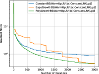
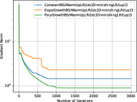
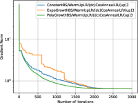
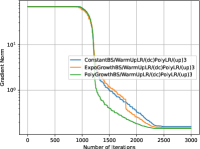
Figure 9: Norm of the gradient of the objective function against number of iterations for warm-up LRs that have an increasing part with three increments on COIL100 dataset.

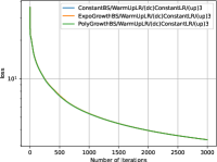
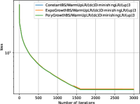
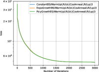
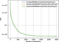
Figure 10: Objective function value against number of iterations for warm-up LRs that have an increasing part with three increments on COIL100 dataset.

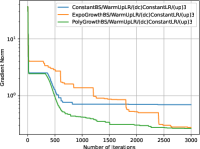
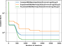
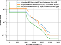
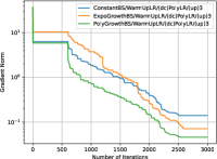
Figure 11: Norm of the gradient of the objective function against number of iterations for warm-up LRs that have an increasing part with three increments on MNIST dataset.

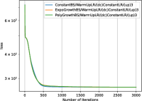
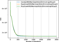
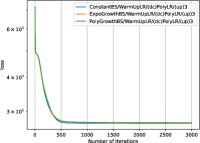
Figure 12: Objective function value against number of iterations for warm-up LRs that have an increasing part with three increments on MNIST dataset.

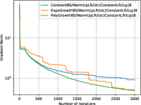
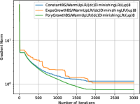
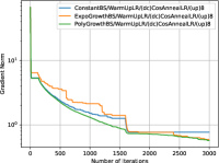
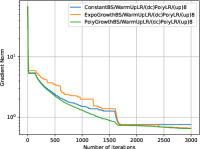
Figure 13: Norm of the gradient of the objective function against number of iterations for warm-up LRs that have an increasing part with eight increments on COIL100 dataset.

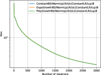
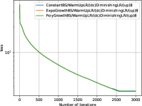
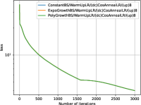
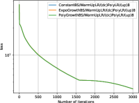
Figure 14: Objective function value against number of iterations for warm-up LRs that have an increasing part with eight increments on COIL100 dataset.

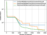
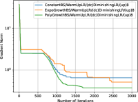
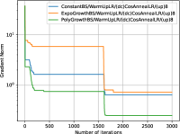
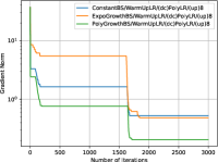
Figure 15: Norm of the gradient of the objective function against number of iterations for warm-up LRs that have an increasing part with eight increments on MNIST dataset.

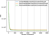
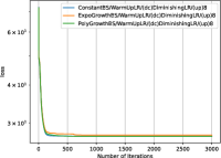
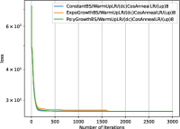
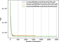
Figure 16: Objective function value against number of iterations for warm-up LRs that have an increasing part with eight increments on MNIST dataset.

$\textbf{[Case A:]}\quad l=l_{w}=3$
Figures 9 and 11 plot performance in terms of the gradient norm of the objective function against the number of iterations for a warm-up LR with decay parts (1), (2), (3), and (4) on the COIL100 and MNIST datasets, respectively. Figures 10 and 12 plot performance in terms of the objective function value against the number of iterations for a warm-up LR with decay parts (1), (2), (3), and (4) for the COIL100 and MNIST datasets, respectively. Figures 9 and 11 show that using an increasing batch size accelerates RSGD convergence. However, as shown in Figures 10 and 12, the differences in the objective function values are small. As mentioned in Section 5, this may be because the objective function is flat around the optimal solution.

$\textbf{[Case B:]}\quad l=3,l_{w}=8$
Figures 13 and 15 plot the performance in terms of the gradient norm of the objective function against the number of iterations for a warm-up LR with decay parts (1), (2), (3), and (4) for the COIL100 and MNIST datasets, respectively. Figures 14 and 16 plot the performance in terms of the objective function value against the number of iterations of a warm-up LR with decay parts (1), (2), (3), and (4) for the COIL100 and MNIST datasets, respectively. Figures 13 and 15 show that using an increasing batch size accelerates RSGD convergence. However, as shown in Figures 14 and 16, the differences in the objective function values are small. As mentioned in Section 5, this may be because the objective function is flat around the optimal solution.

B.2 Low-rank Matrix Completion

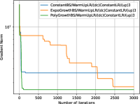
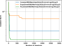
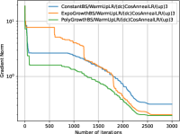
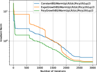
Figure 17: Norm of the gradient of the objective function against number of iterations for warm-up LRs that have an increasing part with three increments on MovieLens-1M dataset.

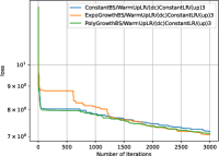
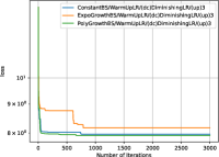
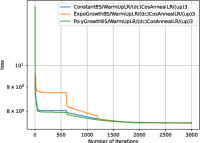
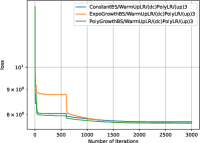
Figure 18: Objective function value against number of iterations for warm-up LRs that have an increasing part with three increments on MovieLens-1M dataset.

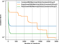
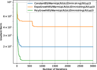
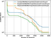
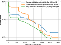
Figure 19: Norm of the gradient of the objective function against number of iterations for warm-up LRs that have an increasing part with three increments on Jester dataset.

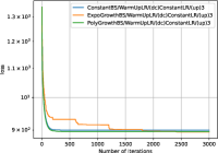
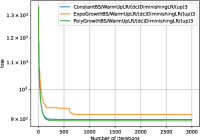
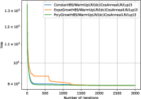
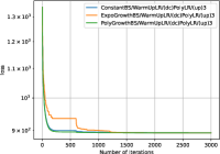
Figure 20: Objective function value against number of iterations for warm-up LRs that have an increasing part with three increments on Jester dataset.

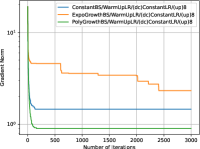
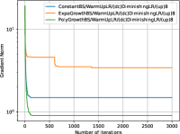
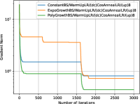
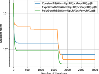
Figure 21: Norm of the gradient of the objective function against number of iterations for warm-up LRs that have an increasing part with eight increments on MovieLens-1M dataset.

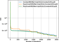
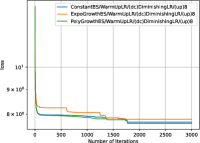
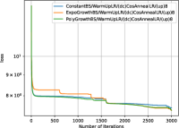
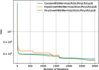
Figure 22: Objective function value against number of iterations for warm-up LRs that have an increasing part with eight increments on MovieLens-1M dataset.

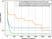
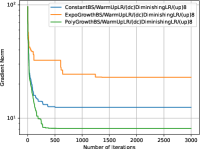
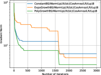
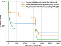
Figure 23: Norm of the gradient of the objective function against number of iterations for warm-up LRs that have an increasing part with eight increments on Jester dataset.

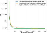
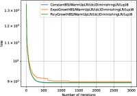
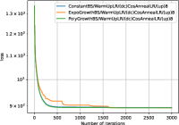
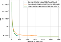
Figure 24: Objective function value against number of iterations for warm-up LRs that have an increasing part with eight increments on Jester dataset.

$\textbf{[Case C:]}\quad l=l_{w}=3$
Figures 17 and 19 plot the performance in terms of the gradient norm of the objective function against the number of iterations for a warm-up LR with decay parts (1), (2), (3), and (4) on the MovieLens-1M and Jester datasets, respectively. Figures 17 and 20 plot the performance in terms of the objective function value against the number of iterations for a warm-up LR with decay parts (1), (2), (3), and (4) on the MovieLens-1M and Jester datasets, respectively. Figures 17 and 19 show that using an increasing batch size accelerates RSGD convergence. As shown in Figures 18 and 20, the objective function value was slightly lower when using an increasing batch size compared with using a constant batch size.

$\textbf{[Case D:]}\quad l=3,l_{w}=8$
Figures 21 and 23 plot the performance in terms of the gradient norm of the objective function against the number of iterations for a warm-up LR with decay parts (1), (2), (3), and (4) on the MovieLens-1M and Jester datasets, respectively. Figures 21 and 24 plot the performance in terms of the objective function value against the number of iterations for a warm-up LR with decay parts (1), (2), (3), and (4) on the MovieLens-1M and Jester datasets, respectively. Figures 21 and 23 show that using an increasing batch size accelerates RSGD convergence. As shown in Figures 22 and 24, the objective function value was slightly lower when using an increasing batch size compared with using a constant batch size.

The results of experiments on the COIL100 and MNIST datasets (Cases A, B) and the MovieLens-1M and Jester datasets (Cases C, D) show that using an exponential growth BS tends to be less effective with a diminishing LR. From Figure 6, as mentioned in Section 5, using an increasing batch size tends to be less effective. However, with the MovieLens-1M dataset in Case C, using an increasing batch size resulted in better performance than using a constant batch size. Moreover, when using a warm-up LR, unlike with the other LRs, using an exponential growth BS resulted in more stable and better performance compared with using a constant BS.

References

• Absil et al. (2008) Absil, P.-A., Mahony, R., and Sepulchre., R. Optimization Algorithms on Matrix Manifolds. Princeton University Press, 2008.
• Bécigneul & Ganea (2019) Bécigneul, G. and Ganea, O. Riemannian adaptive optimization methods. In International Conference on Learning Representations, 2019.
• Bonnabel (2013) Bonnabel, S. Stochastic gradient descent on riemannian manifolds. IEEE Transactions on Automatic Control, 58(9):2217–2229, 2013.
• Boumal (2023) Boumal, N. An introduction to optimization on smooth manifolds. Cambridge University Press, 2023.
• Boumal & Absil (2015) Boumal, N. and Absil, P.-A. Low-rank matrix completion via preconditioned optimization on the grassmann manifold. Linear Algebla and its Applications, 475:200–239, 2015.
• Breloy et al. (2021) Breloy, A., Kumar, S., Sun, Y., and Palomar, D. P. Majorization-minimization on the stiefel manifold with application to robust sparse pca. IEEE Transactions on Signal Processing,, 69:1507–1520, 2021.
• Cai et al. (2022) Cai, J. F., Li, J., and Xia, D. Generalized low-rank plus sparse tensor estimation by fast riemannian optimization. Journal of the American Statistical Association, 2022.
• Chami et al. (2019) Chami, I., Ying, Z., Ré, C., and Leskovec, J. Hyperbolic graph convolutional neural networks. In Advances in Neural Information Processing Systems, 2019.
• Chen et al. (2018) Chen, L., Papandreou, G., Kokkinos, I., Murphy, K., and Yuille, A. L. Deeplab: Semantic image segmentation with deep convolutional nets, atrous convolution, and fully connected crfs. IEEE Trans. Pattern Anal. Mach. Intell., 40(4):834–848, 2018.
• Chen et al. (2017) Chen, X., Weng, J., Lu, W., Xu, J., and Weng, J. Deep manifold learning combined with convolutional neural networks for action recognition. IEEE transactions on neural networks and learning systems, 29(9):3938–3952, 2017.
• Chen et al. (2024) Chen, Z., Song, Y., Liu, G., Kompella, R. R., Wu, X., and Sebe, N. Riemannian multinomial logistics regression for SPD neural networks. In IEEE/CVF Conference on Computer Vision and Pattern Recognition, pp.  17086–17096. IEEE, 2024.
• Criscitiello & Boumal (2023) Criscitiello, C. and Boumal, N. Curvature and complexity: Better lower bounds for geodesically convex optimization. In The Thirty Sixth Annual Conference on Learning Theory, 2023.
• Durmus et al. (2021) Durmus, A., Jiménez, P., Moulines, E., and Said, S. On riemannian stochastic approximation schemes with fixed step-size. In The 24th International Conference on Artificial Intelligence and Statistics, 2021.
• Fei et al. (2023) Fei, Y., Wei, X., Liu, Y., Li, Z., and Chen, M. A survey of geometric optimization for deep learning: From euclidean space to riemannian manifold. arXiv, 2023.
• Goldberg et al. (2001) Goldberg, K. Y., Roeder, T., Gupta, D., and Perkins, C. Eigentaste: A constant time collaborative filtering algorithm. Inf. Retr., 4(2):133–151, 2001.
• Han & Gao (2022) Han, A. and Gao, J. Improved variance reduction methods for riemannian non-convex optimization. IEEE Transactions on Pattern Analysis and Machine Intelligence, 44(11):7610–7623, 2022.
• Harper & Konstan (2016) Harper, F. M. and Konstan, J. A. The movielens datasets: History and context. ACM Trans. Interact. Intell. Syst., 5(4):19:1–19:19, 2016.
• He et al. (2016) He, K., Zhang, X., Ren, S., and Sun, J. Deep residual learning for image recognition. In 2016 IEEE Conference on Computer Vision and Pattern Recognition, pp.  770–778. IEEE Computer Society, 2016.
• He et al. (2024) He, Y., Tiwari, G., Birdal, T., Lenssen, J. E., and Pons-Moll, G. NRDF: neural riemannian distance fields for learning articulated pose priors. In IEEE/CVF Conference on Computer Vision and Pattern Recognition, pp.  1661–1671. IEEE, 2024.
• Hoffer et al. (2017) Hoffer, E., Hubara, I., and Soudry, D. Train longer, generalize better: closing the generalization gap in large batch training of neural networks. In Advances in Neural Information Processing Systems, 2017.
• Hosseini & Sra (2015) Hosseini, R. and Sra, S. Matrix manifold optimization for gaussian mixtures. In Advances in Neural Information Processing Systems, pp.  910–918, 2015.
• Hosseini & Sra (2020) Hosseini, R. and Sra, S. An alternative to EM for gaussian mixture models: batch and stochastic riemannian optimization. Math. Program., 181(1):187–223, 2020.
• Hu et al. (2020) Hu, J., Liu, X., Wen, Z.-W., and Yuan, Y.-X. A brief introduction to manifold optimization. Journal of the Operations Research Society of China, 8(2):199–248, 2020.
• Huang et al. (2017) Huang, Z., Wan, C., Probst, T., and Van Gool, L. Deep learning on lie groups for skeleton-based action recognition. In Proceedings of the IEEE conference on computer vision and pattern recognition, 2017.
• Hundt et al. (2019) Hundt, A., Jain, V., and Hager, G. D. sharpdarts: Faster and more accurate differentiable architecture search. arXiv, 2019.
• Ji et al. (2023) Ji, C., Fu, Y., and He, P. Adaptive riemannian stochastic gradient descent and reparameterization for gaussian mixture model fitting. In Asian Conference on Machine Learning, 2023.
• Kasai & Mishra (2016) Kasai, H. and Mishra, B. Low-rank tensor completion: a riemannian manifold preconditioning approach. In Proceedings of the 33nd International Conference on Machine Learning, 2016.
• Kasai et al. (2018) Kasai, H., Sato, H., and Mishra, B. Riemannian stochastic recursive gradient algorithm. In Proceedings of the 35th International Conference on Machine Learning, 2018.
• Kasai et al. (2019) Kasai, H., Jawanpuria, P., and Mishra, B. Riemannian adaptive stochastic gradient algorithms on matrix manifolds. In the 36th International Conference on Machine Learning, 2019.
• Keskar et al. (2017) Keskar, N. S., Mudigere, D., Nocedal, J., Smelyanskiy, M., and Tang, P. T. P. On large-batch training for deep learning: Generalization gap and sharp minima. In International Conference on Learning Representations, 2017.
• Kim & Yang (2022) Kim, J. and Yang, I. Nesterov acceleration for riemannian optimization. arXiv, 2022.
• Krizhevsky et al. (2012) Krizhevsky, A., Sutskever, I., and Hinton, G. E. Imagenet classification with deep convolutional neural networks. In Advances in Neural Information Processing Systems, 2012.
• LeCun et al. (1998) LeCun, Y., Cortes, C., and Burges, C. The mnist database of handwritten digits. http://yann.lecun.com/exdb/mnist, 1998.
• Lee (1997) Lee, J. M. Riemannian Manifolds: An Introduction to Curvature. Springer-Verlag New York, 1997.
• Lewkowycz (2021) Lewkowycz, A. How to decay your learning rate. arXiv, 2021.
• Lin et al. (2020a) Lin, T., Fan, C., Ho, N., Cuturi, M., and Jordan, M. Projection robust wasserstein distance and riemannian optimization. In Advances in Neural Information Processing Systems, 2020a.
• Lin et al. (2020b) Lin, T., Stich, S. U., Patel, K. K., and Jaggi, M. Don’t use large mini-batches, use local SGD. In 8th International Conference on Learning Representations, 2020b.
• Liu & Boumal (2020) Liu, C. and Boumal, N. Simple algorithms for optimization on riemannian manifolds with constraints. Applied Mathematics & Optimization, 2020.
• Liu et al. (2020) Liu, L., Jiang, H., He, P., Chen, W., Liu, X., Gao, J., and Han, J. On the variance of the adaptive learning rate and beyond. In International Conference on Learning Representations, 2020.
• Liu et al. (2019) Liu, Q., Nickel, M., and Kiela, D. Hyperbolic graph neural networks. In Advances in Neural Information Processing Systems, 2019.
• Liu et al. (2015) Liu, X., Wang, X., and Wang, W. Maximization of matrix trace function of product stiefel manifolds. SIAM J. Matrix Anal. Appl., 36(4):1489–1506, 2015.
• Liu et al. (2017) Liu, Y., Shang, F., Cheng, J., Cheng, H., and Jiao, L. Accelerated first-order methods for geodesically convex optimization on riemannian manifolds. In Advances in Neural Information Processing Systems, 2017.
• Liu et al. (2021) Liu, Z., Lin, Y., Cao, Y., Hu, H., Wei, Y., Zhang, Z., Lin, S., and Guo, B. Swin transformer: Hierarchical vision transformer using shifted windows. In IEEE/CVF International Conference on Computer Vision, pp.  9992–10002. IEEE, 2021.
• Loshchilov & Hutter (2017) Loshchilov, I. and Hutter, F. SGDR: Stochastic gradient descent with warm restarts. In International Conference on Learning Representations, 2017.
• McCandlish et al. (2018) McCandlish, S., Kaplan, J., Amodei, D., and Team, O. D. An empirical model of large-batch training. arXiv, 2018.
• Nene et al. (1996) Nene, S. A., Nayar, S. K., Murase, H., and et al. Columbia object image library (coil-100). Technical report, Columbia University, 1996. CUCS-006-96.
• Nguyen et al. (2019) Nguyen, L. T., Kim, J., and Shim, B. Low-rank matrix completion: A contemporary survey. IEEE Access, 7:94215–94237, 2019.
• Robbins & Monro (1951) Robbins, H. and Monro, S. A stochastic approximation method. The Annals of Mathematical Statistics, 22(3):400–407, 1951.
• Roy et al. (2018) Roy, S. K., Mhammedi, Z., and Harandi, M. Geometry aware constrained optimization techniques for deep learning. In Proceedings of the IEEE/CVF Conference on Computer Vision and Pattern Recognition, 2018.
• Rudin (1976) Rudin, W. Principles of Mathematical Analysis (3rd Ed). McGraw Hill Higher Education, 1976.
• Sakai & Iiduka (2024) Sakai, H. and Iiduka, H. Convergence of riemannian stochastic gradient descent on hadamard manifold. Pacific Journal of Optimization, 20(4):743–767, 2024.
• Sakai & Iiduka (2025) Sakai, H. and Iiduka, H. A general framework of riemannian adaptive optimization methods with a convergence analysis. Transactions on Machine Learning Research, 2025. ISSN 2835-8856.
• Sato & Iiduka (2024) Sato, N. and Iiduka, H. Using stochastic gradient descent to smooth nonconvex functions: Analysis of implicit graduated optimization. arXiv, 2024.
• Sun et al. (2017) Sun, J., Qu, Q., and Wright, J. Complete dictionary recovery over the sphere II: recovery by riemannian trust-region method. IEEE Trans. Inf. Theory, 63(2):885–914, 2017.
• Tagare (2011) Tagare, H. D. Notes on stiefel manifolds, 2011. URL https://noodle.med.yale.edu/hdtag/notes/steifel_notes.pdf.
• Tripuraneni et al. (2018) Tripuraneni, N., Flammarion, N., Bach, F., and Jordan, M. I. Averaging stochastic gradient descent on Riemannian manifolds. In Proceedings of the 31st Conference On Learning Theory, 2018.
• Umeda & Iiduka (2024) Umeda, H. and Iiduka, H. Increasing both batch size and learning rate accelerates stochastic gradient descent. arXiv, 2024.
• Vandereycken (2013) Vandereycken, B. Low-rank matrix completion by riemannian optimization. SIAM J. Optim., 23(2):1214–1236, 2013.
• Wang et al. (2020) Wang, J., Chen, Y., Chakraborty, R., and Yu, S. X. Orthogonal convolutional neural networks. In Proceedings of the IEEE/CVF conference on computer vision and pattern recognition, 2020.
• Weber & Sra (2023) Weber, M. and Sra, S. Riemannian optimization via frank-wolfe methods. Math. Program., 199(1):525–556, 2023.
• Wu et al. (2014) Wu, Y., Holland, D. J., Mantle, M. D., Wilson, A. G., Nowozin, S., Blake, A., and Gladden, L. F. A bayesian method to quantifying chemical composition using NMR: application to porous media systems. In European Signal Processing Conference, 2014.
• You et al. (2020) You, Y., Li, J., Reddi, S. J., Hseu, J., Kumar, S., Bhojanapalli, S., Song, X., Demmel, J., Keutzer, K., and Hsieh, C. Large batch optimization for deep learning: Training BERT in 76 minutes. In International Conference on Learning Representations, 2020.
• Yun & Yang (2023) Yun, J. and Yang, E. Riemannian SAM: sharpness-aware minimization on riemannian manifolds. In Advances in Neural Information Processing Systems, 2023.
• Zhang & Sra (2016) Zhang, H. and Sra, S. First-order methods for geodesically convex optimization. In Proceedings of the 29th Conference on Learning Theory, 2016.
• Zhang et al. (2016) Zhang, H., J. Reddi, S., and Sra, S. Riemannian svrg: Fast stochastic optimization on riemannian manifolds. In Advances in Neural Information Processing Systems, 2016.
• Zhu et al. (2020) Zhu, S., Pan, S., Zhou, C., Wu, J., Cao, Y., and Wang, B. Graph geometry interaction learning. Advances in Neural Information Processing Systems, 2020.