There is Room at the Top: Fundamental Quantum Limits for Detecting Ultra-high Frequency Gravitational Waves

Abstract

The sky of astrophysical gravitational waves is expected to be quiet above $\sim 10{\rm kHz}$, which is the upper limit of characteristic frequencies of dynamical processes involving astrophysical black holes and neutron stars. Therefore, the ultrahigh ($\geq 10{\rm kHz}$) frequency window is particularly promising for detecting primordial gravitational waves, as isolating the contribution from the astrophysical foreground has always been a challenging problem for gravitational wave background detection at ${\rm nHz,mHz}$ and the audio band studied so far. While there are various types of detectors proposed targeting the ultra-high frequency gravitational waves, they have to satisfy the (loss-constrained) fundamental limits of quantum measurements. We develop a universal framework for the quantum limit under different measurement schemes and input quantum states, and apply them to several plausible detector configurations. The fundamental limits are expressed as the strength of gravitational wave background at different frequencies, which should serve as a lower limit for ultra-high frequency gravitational wave signal possibly detectable, to probe early-universe phase transitions, and/or other primordial gravitational wave sources. We discover that a GUT-motivated phase transition from $10^{7}-10^{10}\,\rm{GeV}$ can naturally lead to possibly detectable GW signals within the band of $\rm{kHz-MHz}$. For phase transition above $10^{10}\,\rm{GeV}$, the signals are however below the quantum limit and are thus not detectable. Ultra-high frequency GWs also provide a window to test topological defects such as domain walls and cosmic strings generated close to the GUT scale.

I Introduction

Since the first detection of the binary black hole merger event GW150914 [1], the LIGO-Virgo and KAGRA collaboration has achieved tremendous success in detecting more than 100 compact binary mergers in the audio band [2]. The most recent Pulsar Timing Array measurements also show promising tentative evidence of gravitational wave background in the ${\rm n}$Hz band [3, 4, 5, 6]. In the next decade, spaceborne detectors such as LISA (Laser Interferometer Space Antenna), Taiji, and Tianqin [7, 8, 9], are likely to detect gravitational waves in the ${\rm m}$Hz range. This is a good time for the astronomy community to consider the science potential of probing gravitational waves in other frequency bands and the best observation technique(s).

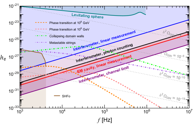
Figure 1: Fundamental quantum limits for different experimental setups at frequency range $10^{3}{\rm Hz}-10^{7}{\rm Hz}$, with integration time of $10$ year and frequency bin width of $1{\rm k}$Hz. A representative astrophysical foreground from binary neutron star mergers is also included (assuming the equation of state SHFo [10], data extracted from [11]), which decays rapidly over $4{\rm k}$Hz. At ultra-high frequency, there is minimal contribution of astrophysical sources, clearing the way to detect effects of GUT-induced phase transitions (B1 at $10^{8}$ GeV, B2 at $10^{9}$ GeV), collapsing domain walls (B3) or metastable strings (B4).

In order to produce higher frequency gravitational waves, we generally require astronomical objects with higher curvatures, i.e. more massive neutron stars and lighter black holes. According to their astrophysical formation channels through supernovae explosions, accretion, and binary mergers, together with neutron star equation-of-state constraints, the maximum mass of a neutron star and a minimum mass of an astrophysical black hole are likely in the $2-3M_{\odot}$ range [12, 13, 14], with the corresponding major dynamical frequencies $\leq 10{\rm k}$Hz. Above this frequency, the foreground astrophysical gravitational wave, which effectively sets the final detection limits for primordial waves in the audio band [15], is greatly suppressed. Therefore this ultra-high frequency band becomes a “golden window” to probe gravitational waves from the early universe, phase transitions, topological defects, and/or other origins [16].

Laser interferometers have reached quantum-limited measurement accuracy and have proven extremely successful in detecting gravitational waves in the audio band. For ultrahigh frequencies $\geq 10{\rm k}$ Hz, in addition to laser interferometer, there are also several proposals using microwave-cavities and cavity-assisted levitating spheres. However, it is yet unclear what the optimal design and the best measurement accuracy would be. In order to guide future studies in this direction, i.e., what kind of theoretical models can be tested in this frequency band, we provide a unified framework to determine the ultimate measurement precision from a quantum-limited measurement perspective. We apply an energetic quantum limit (as constrained by loss) to various viable proposals to set their ultimate measurement precision, with all classical noises excluded. Gravitational waves under such limit are likely not detectable based on current understanding. As an application of such detection limit, we analyze major Grand Unification Model(s) and present the parameter range that may be tested by detectors saturating the fundamental limit.

II Fundamental limits

Despite their apparent differences in physical layouts, all high-frequency detectors proposed so far can be unified within the same framework, due to their shared mathematical description for analyzing ultimate measurement precision and their common core element: the electromagnetic resonator.

Mathematically, measurement precision can be analyzed by treating the detection process as a quantum estimation problem [17]. At high frequencies, the stochastic GW signal introduces random shift in the quantum state of the detector. The magnitude is quantified by the excess variance:

$$\sigma^{2}(f)=|G(f)|^{2}\,h^{2}(f)\,,$$ (1)

where the gain $G$ quantifies detector’s response to the GW strain $h$ at the frequencies $f$. The accuracy for estimating the excess variance, quantified by the signal-to-noise ratio (SNR), is determined by the quantum state of the system and also the measurement scheme that measures the quantum state. Fundamental quantum limits to the SNR for different detectors are summarized in Table 1.

System	Measurement	SNR	$\mathbf{h_{c,\text{min}}^{2}(f)}$	Optimal Size $L$	Energy $\bar{\mathcal{E}}$	Dominant Noise
Laser	linear measurement	${\sigma^{2}}{\epsilon}^{-1}\sqrt{N}$	$\epsilon S_{n}^{\rm vac}(f)N^{-\frac{1}{2}}$	$c/4f_{0}$	${2{\rm P}_{\rm arm}L}/{c}$	cavity loss
Inter-	photon counting	${\sigma}\sqrt{N}$	$2S_{n}^{\rm vac}(f)N^{-1}$			quantum vacuum
ferometer	optimal	${\sigma}{\epsilon}^{-1}\sqrt{N}$	$2\epsilon S_{n}^{\rm vac}(f)N^{-1}$			cavity loss
EM Cavity	linear	$\sigma^{2}\sqrt{N}$	$S_{n}^{\rm vac}(f)(N)^{-\frac{1}{2}}$	$c/f_{0}$	${B_{0}^{2}}V/{2\mu_{0}}$	quantum vacuum
Levitating Sphere	linear	${\sigma^{2}}{\epsilon}^{-1}\sqrt{N}$	$\epsilon S_{n}^{\rm vac}(f)(N)^{-\frac{1}{2}}$	$\gg c/2f_{0}$	${2{\rm P}_{\rm arm}L}/{c}$	cavity loss

Table 1: SNR and minimum detectable threshold of different proposals for weak stochastic signal, normalized by the excess variance $\sigma$ and vacuum shot noise level, $S_{n}^{\rm vac}(f)=\frac{f\,\hbar^{2}}{\alpha^{2}(f)\cdot\bar{S}_{\cal EE}^{\rm vac}(f)}$, respectively. The measurement scheme and key physical features of each proposal is also presented. Here, $\epsilon=\epsilon(f)$ is the system’s loss level, quantified by the decoherence rate, $N$ is the number of samples, defined as $N=T_{\rm int}\,\Delta f$, with $T_{\rm int}$ being the integration time and $\Delta f$ the frequency band of interest, $f_{0}$ is the frequency of targeting signal, ${\rm P}_{\rm arm}$ is the circulating power in arm cavity, $B_{0}$ and $V$ is the static magnetic field and total volume of the resonant cavity.

Physically, for all proposed detectors, GWs are coupled to an electromagnetic cavity or resonator, which resonantly enhances the strain signal. The coupling Hamiltonian can be described as:

$$\hat{H}_{\rm int}=A\,h\,\hat{\cal E}_{EM}\,.$$ (2)

Here $\alpha<1$ describes the antenna response; $h$ is the magnitude GW strain; ${\cal E}_{EM}$ is the energy of the electromagnetic field of the detector. The energy fluctuation at the quantum level provides a universal bound to the signal gain $G$ [18, 19]:

$$|G(f)|^{2}=\alpha^{2}\frac{\bar{S}_{\cal EE}^{\,\rm vac}(f)}{\hbar^{2}}\,.$$ (3)

This can be intuitively understood by the energy-time uncertainty principle: detectors with larger energy fluctuations exhibit greater sensitivity to space-time variations. In this formula, $\bar{S}_{\cal EE}^{\,\rm vac}$ is the spectral density of the quantum energy fluctuations driven by vacuum noise. It is given by

$$\bar{S}^{\text{vac}}_{\cal EE}(f)=\bar{\cal E}\sum_{k}S_{k}^{\rm vac}=\bar{\cal E}\sum_{k}\frac{2\hbar(\omega_{0}+\Delta_{k})\gamma_{k}}{(2\pi f-|\Delta_{k}|)^{2}+\gamma_{k}^{2}}\,.$$ (4)

The energy fluctuation is a summation of Lorentzian-shaped spectra of individual cavity modes ($\omega_{0}$ is the carrier frequency, $\gamma_{k}$ is the bandwidth and $\Delta_{k}$ is the resonant frequency), and proportional to $\bar{\cal E}$, the total energy stored in the system.

Given the above physical constraint of the gain, we can then convert the fundamental limit for the SNR to the minimum detectable threshold of the characteristic strain:

$$h^{2}_{\rm c,min}(f)\equiv f\cdot h^{2}(f)|_{\rm SNR=1}\,.$$ (5)

The result is also presented in Table 1. Numerical results of $h_{\rm c,min}$ for different proposed detectors are illustrated in Fig. 1. In the study of stochastic GW background, a commonly used parameter is the GW energy density spectrum $\Omega_{\rm{GW}}(f)$. It relates to the characteristic strain via: $\Omega_{\rm{GW}}(f)=2\pi^{2}/(3H_{0}^{2})f^{2}h_{c}^{2}(f)$ where $H_{0}=100{\rm h}~{\rm km/s/Mpc}$ is the Hubble constant. In order to define the ultimate measurement precision, we only consider the quantum noise of detectors, including the quantum fluctuation of the ideal state and intrinsic loss of the system achievable with the state-of-the-art technology. Meanwhile, each sensitivity curve in Fig. 1 is an envelope that contains the peak sensitivities of many individual detectors. Key features of each detector design in summarized in Table. 1. Detailed physical layout and parameter settings for each proposal are provided in the Appendix A.3.

III Implications

Based on the quantum-limited sensitivity on high-frequency GW detection, we discuss the implications on how well one can test some of the well-motivated predictions related to Grand Unified Theories (GUTs) and topological defects (domain walls and cosmic strings).

GUT-motivated phase transition: GUTs, which aim to unify the three fundamental particle forces, can naturally predict cosmological phase transitions at ultra-high energy scales. While the energy scale of GUT breaking ($\gtrsim 10^{16}$ GeV) is prohibitively high, intermediate symmetry breaking can naturally occur at lower scales but sufficiently higher than the electro-weak scale. The SO(10) framework [20] provides plenty of such possibilities and we highlight those symmetries in orange in Fig. 2. Note that these symmetries are necessarily intermediate symmetries as required by gauge unification with scales sufficiently lower than the GUT scale. In particular, we focus on intermediate symmetries with breaking scales in the range of $10^{6}\sim 10^{10}$ GeV. Two representative benchmarks of GW spectra at $10^{8}$ GeV (B1) and $10^{9}$ GeV (B2) are shown in the right panel of Fig. 1, which can be resulted in typical symmetry breaking $G_{422}\to G_{3221}$ or $G_{3221}\to G_{\rm SM}$ shown in Fig. 2. Earlier results of GWs induced by Pati-Salam symmetry breaking without embedding in a full $SO(10)$ framework can be found in [21, 22].

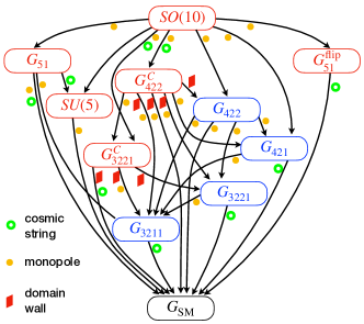
Figure 2: Non-SUSY $SO(10)$ GUT breaking chains as motivations of ultra-high frequency GWs via phase transition. Conventions, e.g., $G_{422}=SU(4)_{c}\times SU(2)_{L}\times SU(2)_{R}$, are understood [23]. $G_{\rm SM}\equiv SU(3)\times SU(2)_{L}\times U(1)_{Y}$ denotes the gauge symmetry of the Standard Model. Topological defects (cosmic strings, monopoles and domain walls) associated with the symmetry breaking [24] are marked. Gauge symmetries which might provide phase transition at scales lower than $10^{10}$ GeV and consistent with cosmological observations are highlighted in blue.

The intermediate symmetry breaking can be triggered by a Higgs-like mechanism, involving a scalar field that acquires a vacuum expectation value (VEV). The symmetry breaking is accompanied by a cosmological phase transition at very high temperature $T_{*}$ in the early Universe. Its dynamics are described by the effective potential, which is dressed by zero-temperature and finite-temperature loop corrections of particles (gauge bosons, scalars and fermions) participating in the phase transition. The potential is determined once the details of a model are provided. In particular, we show in Appendix 2.3 analytical connections between parameters in phase transition and particle models in the GUT framework.

During a first-order phase transition, the energy stored in the false vacuum is drastically released into the bulk through bubble nucleation, generating gravitational radiation. The latter contributes as a stochastic GW background observed today. For phase transitions that involve gauge symmetry breaking, the sound waves in the bulk plasma are considered as the primary source of GWs. The acoustic GW power spectrum today is [25, 26]:

$${\rm{h}}^{2}\Omega_{\text{GW}}(f) ={\rm{h}}^{2}\Omega_{\text{p}}\Big{(}\frac{f}{f_{\text{p}}}\Big{)}^{\!3}\left[\frac{4}{7}+\frac{3}{7}\Big{(}\frac{f}{f_{\text{p}}}\Big{)}^{\!2}\right]^{-\frac{7}{2}},$$ (6)

with the peak frequency and peak amplitude given by

$$f_{\text{p}} \simeq 89\,\text{kHz}\,v_{w}^{-1}\Big{(}\frac{g_{*}}{100}\Big{)}^{\!\frac{1}{6}}\Big{(}\frac{T_{*}}{10^{9}\,\text{GeV}}\Big{)}\Big{(}\frac{\tilde{\beta}}{10^{3}}\Big{)},$$ (7)

$${\rm{h}}^{2}\Omega_{\text{p}} \simeq 1.19\cdot 10^{-9}v_{w}\Big{(}\frac{10^{3}}{\tilde{\beta}}\Big{)}\Big{(}\frac{\kappa_{\rm{sw}}(\alpha)\,\alpha}{1+\alpha}\Big{)}^{\!2}\Big{(}\frac{100}{g_{*}}\Big{)}^{\!\frac{1}{3}}\,,$$

where $\rm{h}$ is the reduced Hubble parameter and it has nothing do to with the strain. Here $T_{*}$ denotes the temperature at the phase transition, $v_{w}$ represents the bubble wall velocity and $g_{*}$ characterizes the number of degrees of freedom (DOF) participating the phase transition. The peak amplitude is determined primarily by two parameters: $\alpha$, which quantifies the energy released into the plasma normalized by the radiation energy, and $\tilde{\beta}$, which represents the inverse duration of the phase transition. Furthermore, $\kappa_{\rm{sw}}(\alpha)$ is an $\alpha$ dependent efficiency factor where an additional suppression factor due to the length of the sound-wave period is encoded[27, 28]. The precise definitions of these parameters are given in Appendix B.1.

GWs in the kilohertz band are naturally achieved via a phase transition at $10^{7}$ GeV while MHz GWs might be realized via a $10^{10}$ GeV scale phase transition. B1 is an ideal example to be tested in the future once the sensitivity can approach the quantum limit. For comparison, B2 shows both the peak and UV bands below the quantum limit, although the IR band is within the detectable region. As its spectrum shape cannot be determined, even if a GW background were detected, it cannot be directly attribute to an origin of phase transitions. Finally, for intermediate symmetry breaking above $10^{10}$ GeV, the signals are below the quantum limit that forbids any direct detection.

Figure 3: Detection capabilities for GUT-induced phase transitions. The left panel shows the SNR of channel limit for gravitational signals under varying $f_{\text{p}}$ and $\Omega_{\text{p}}$, where we fixed the asymptotic behavior of $\Omega_{\rm GW}\propto 1/f^{d}=1/f^{4}$ at high frequency. Signal-to-noise ratio of other proposals can be estimated as ${\rm SNR}_{\rm pc}=3.16\times 10^{-3}\cdot{\rm SNR}_{\rm channel}$, ${\rm SNR}_{\rm lin\,(EM)}=6.64\times 10^{-8}(1.39\times 10^{-5})\cdot{\rm SNR}^{2}_{\rm channel}$. The corner plot at the right illustrates the confidence interval of parameter estimation of EM cavity and channel limit for a benchmark signal with $(\Omega_{\rm p},\,f_{\rm p},\,d)=(4.0\times 10^{-10},\,1.2\times 10^{4},\,4)$, where ellipses with different color intensities denote confidence intervals for $\sigma,\,2\sigma,\,3\sigma$, respectively. Estimation on the phenomenological parameters $\Omega_{\text{p}}$ and $f_{\text{p}}$ can be translated into two-dimensional constraint on the phase transition parameters in GUT.

Collapsing domain walls: Domain walls provide another mechanism for ultra-high-frequency gravitational waves. The domain wall is a topological defect that is inevitably generated after spontaneous breaking of discrete symmetries. The latter are frequently applied in beyond the Standard Model new physics models at ultra-high energy scales. Domain walls, once they are generated, appear as two-dimensional massive objects evolving in the universe. In order to avoid a domain-wall-dominated Universe, a bias term, originating from an asymmetry, is often introduced to break the degeneracy between vacuum states. They cause the walls to collapse during which period GWs are generated. The spectrum of GWs from collapsing domain walls follows broken power laws of $f^{3}$ on the IR band and roughly $f^{-1}$ on the UV band, and the peak frequency is determined by the annihilation temperature [29]. Ultra-high-frequency GWs in the kHz-MHz band arise from discrete symmetry breaking at scales ranging from $10^{9}\,\rm{GeV}$ to the GUT scale, provided suitable bias terms are included [30]. A benchmark of domain walls (B3) with tension (i.e., surface energy) $\sigma\sim(10^{14}~{\rm GeV})^{3}$ is presented in the green curve in Fig. 1. Collapsing domain walls are not predicted in GUTs. Some New Physics frameworks that naturally achieve it include: residual $Z_{N}$ symmetry $\sim 10^{12}$ GeV arising in axion models to address strong CP problem [31] and discrete symmetries (either Abelian [32] or non-Abelian [33]) in solving the problem of quark and lepton flavor mixing [34, 35].

Metastable strings: Cosmic strings are generated after the spontaneous breaking of $U(1)_{B-L}$. The latter is naturally predicted in Pati-Salam or relevant GUT frameworks [36], explaining the tiny mass of neutrino with a Majorana nature in the seesaw framework [37, 38]. Cosmic strings form a network in the early Universe, intersecting to form loops that oscillate and emit GWs as they shrink [39]. Simulations suggest the GW spectrum from stable cosmic strings spans nHz to GHz, with a high-frequency plateau proportional to $\sqrt{\mu}$, where $\mu$ is the string’s energy density per unit length [40]. If the $B-L$ breaking scale is not hierarchically far below the GUT scale, strings can decay to monopole-antimonopole pairs, forming a metastable string network [41]. GWs at lower frequency, referring to those released from loops at later time, are suppressed due to the decay of strings. The decay width per string unit length is determined by the ratio $\kappa=m^{2}/\mu$, where $m$ is the GUT monopole mass naturally around the GUT scale. A smaller $\kappa$ means a faster decaying string network, corresponding to a higher frequency cutoff at the IR band. In Fig. 1, we show a benchmark at $\kappa=25$ (B4). The GW spectrum below $10^{4}$ Hz is suppressed and follows the power-law $f^{2}$ until it reaches the plateau round $10^{4}$-$10^{5}$ Hz.

IV Conclusion

In the ultra-high frequency band the universe is free of astrophysical stochastic GW foreground, which is certainly beneficial for probing promordial GWs. While the discussion of best detector configurations in this band is still in the early stage, we propose an unified framework to determine the quantum-limited sensitivity on strain, including proposals with varying coupling Hamiltonian, injected quantum states and readout scheme. The results obtained in Fig. 1 may be considered as the most optimistic bound that can be achieved, as classical noise sources are not included. With these bounds, we find that testing GUT theories with phase transition temperature below $10^{10}\,\rm{GeV}$ is, in principle, allowed by future detectors in this band. Some of the domain-wall models with very large tension may also generate detectable GWs. Most importantly, we expect these bounds may be used to facilitate more studies on models that generate detectable GWs in the ultra-high frequency band.

While preparing the manuscript, we find a related discussion on the sensitivity limit of high frequency detectors in [42], restricted to the linear measurement in the ideal lossless case.

V Acknowledgements

X. G. and H. M. would like to acknowledge the support from the National Key R&D Program of China under the project ’Gravitational Wave Detection’ (Grant No.: 2023YFC2205800) and the support from the Frontier Science Center for Quantum Information. ZWW is supported in part by the National Natural Science Foundation of China (Grant No. 12475105). YLZ was partially supported by National Natural Science Foundation of China (NSFC) under Grant Nos. 12205064, 12347103, and Zhejiang Provincial Natural Science Foundation of China under Grant No. LDQ24A050002. ZWW and YLZ give special thanks to Z.Z. Xing for hospitality in IHEP where the initial collaboration was facilitated.

Appendix A Fundamental quantum limit for detectors

A.1 Energetic quantum limit

In this part, we focus on the energetic quantum limit of general system, that is, its gain to the signal is bounded by the vacuum energy fluctuation inside, and therefore related to the total stored energy. We also dynamically model the impact of quantum loss, extending our discussion to encompass a broader range of systems.

A.1.1 Proof of the upper bound of gain

For a general detection system, the GW signal would introduce a displacement in the out-going quantum state at certain quadrature ($\hat{b}_{\theta}\equiv\hat{b}_{1}\cos\theta+\hat{b}_{2}\sin\theta$)  [19]:

$$\hat{b}_{\theta}(t) =\hat{b}_{\theta}^{(0)}(t)+\int_{-\infty}^{+\infty}\mathrm{d}t^{\prime}G_{\theta}\left(t-t^{\prime}\right)h\left(t^{\prime}\right)$$ (8)

$$\hat{b}_{\theta}(f) =\hat{b}_{\theta}^{(0)}(f)+G_{\theta}(f)h(f)\,,$$

where superscript (0) denotes evolution under a free, time-independent Hamiltonian $\hat{H}_{0}$, and $G_{\theta}$ is a transfer function describing the system’s amplification for strain signal at this quadrature. A system’s gain could be defined as the maximum strain-to-displacement transfer functions across all the possible quadratures:

$$|G(f)|=\sup_{\theta}|G_{\theta}(f)|\,.$$ (9)

With a simple form of interaction Hamiltonian $\hat{H}_{\mathrm{int}}=\alpha h\hat{\cal E}$, the amplification at certain quadrature is given by:

$$G_{\theta}\left(t-t^{\prime}\right)\equiv\frac{i\alpha}{\hbar}\left[\hat{b}_{\theta}^{(0)}(t),\hat{\cal E}^{(0)}\left(t^{\prime}\right)\right]\Theta\left(t-t^{\prime}\right)\,,$$ (10)

which directly yields to an uncertainty principle for continuous measurements[19, 43]:

$$\alpha^{2}(f)\cdot\left[\bar{S}_{b_{\theta}b_{\theta}}(f)\bar{S}_{\cal{E}\cal{E}}(f)-\left|\bar{S}_{b_{\theta}{\cal E}}(f)\right|^{2}\right]\geq{\hbar^{2}}\left|G_{\theta}(f)\right|^{2}\,.$$ (11)

Here, $\bar{S}_{AB}(f)$ represents the symmetrized single-sided spectral correlation, $\bar{S}_{AB}(f)=S_{AB}(f)+S_{BA}(-f)$, where the unsymmetrized correlation $S_{AB}$ is defined by:

$$\operatorname{Tr}\left[\hat{\rho}_{\mathrm{det}}\hat{A}^{(0)}(f)\hat{B}^{(0)\dagger}\left(f^{\prime}\right)\right]\equiv S_{AB}(f)\delta\left(f-f^{\prime}\right).$$ (12)

The equality in Eq. 11 holds for a general Gaussian pure state $\hat{b}_{\theta}^{0}$. Specifically, the special case of vacuum state injection meets the requirement. Maximizing both side of this equation directly gives the exact value of gain:

$$|G(f)|^{2}=\frac{\alpha^{2}(f)}{\hbar^{2}}\sup_{\theta}\left[\bar{S}^{\rm vac}_{b_{\theta}b_{\theta}}(f)\bar{S}^{\rm vac}_{\cal EE}(f)-|\bar{S}^{\rm vac}_{b_{\theta}{\cal E}}(f)|^{2}\right]\,.$$ (13)

Here, we assume a general input-output relationship and linear form of the cavity mode energy:

$$\binom{\hat{b}_{1}(f)}{\hat{b}_{2}(f)} =R(\beta_{2})\left(\begin{array}[]{ll}e^{r}&0\\ 0&e^{-r}\end{array}\right)R(\beta_{1})\binom{\hat{a}_{1}(f)}{\hat{a}_{2}(f)}$$ (14)

$$\hat{\cal E}{(f)} =E_{0}\times\left(\cos\varphi,\sin\varphi e^{i\Delta\psi}\right)\binom{\hat{a}_{1}(f)}{a_{2}(f)}\,,$$

For simplicity, we omit the superscript $(0)$ and an overall phase factor of each. Here, $\hat{a}_{1}(f)=\frac{\hat{a}(f)+\hat{a}^{\dagger}(-f)}{\sqrt{2}}$, $\hat{a}_{2}(f)=\frac{\hat{a}(f)-\hat{a}^{\dagger}(-f)}{\sqrt{2}i}$ is the amplitude and phase quadrature of in-going field respectively, satisfying $\bar{S}_{{a}_{1}{a}_{1}}=\bar{S}_{{a}_{2}{a}_{2}}=1,\bar{S}_{{a}_{1}{a}_{2}}=0$. For the input-output relation, $e^{r}$ describes the level of internal squeezing, with $R(\beta_{1})$ and $R(\beta_{2})$ represents the rotation of state before and after the internal squeezing respectively. Meanwhile, $\varphi$ and $\psi$ basically describes the detector’s dynamical response to external field. With this notation, each term on the right-hand side of Eq. 13 can be expanded into the following form:

$$\bar{S}_{b_{\theta}b_{\theta}}(f) =\left[e^{r}\cos\beta_{1}\cos(\theta-\beta_{2})+e^{-r}\sin\beta_{1}\sin(\theta-\beta_{2})\right]^{2}$$ (15)

$$+\left[-e^{r}\sin\beta_{1}\cos(\theta-\beta_{2})+e^{-r}\cos\beta_{1}\sin(\theta-\beta_{2})\right]^{2}$$

$$\bar{S}_{\cal EE}^{vac}(f) =E_{0}^{2}$$

$$\left|\hat{S}_{b_{\theta}{\cal E}}^{\operatorname{vac}}(f)\right|^{2} =E_{0}^{2}\mid\cos\varphi\left[e^{r}\cos\beta_{1}\cos(\theta-\beta_{2})\right.$$

$$+\left.e^{-r}\sin\beta_{1}\sin(\theta-\beta_{2})\right]+\sin\varphi e^{i\Delta\psi}\times$$

$$\left[\right. \left.-e^{{r}}\sin\beta_{1}\cos(\theta-\beta_{2})+e^{-r}\cos\beta_{1}\sin(\theta-\beta_{2})\right]\left.\right|^{2}\,.$$

Maximizing over $\theta$ gives the analytical expression of gain:

$$|G(f)|^{2}=\frac{\alpha^{2}\ \bar{S}^{\rm vac}_{\cal EE}(f)}{\hbar^{2}}\left[A+\sqrt{A^{2}-B^{2}}\right]\,,$$ (16)

where

$$A =\frac{1}{2}\{\cosh(2r)+[\sin 2\beta_{1}\sin 2\varphi\cos\Delta\psi$$ (17)

$$-\cos 2\beta_{1}\cos 2\varphi]\sinh(2r)\}$$

$$B =\frac{1}{2}\sin 2\varphi\sin\Delta\psi\,.$$

For ultra-high frequency detection, the mechanical back action is usually negligible, corresponding to weak internal squeezing cases with $e^{2r}\approx 1$. In this scenario, Eq. 16 could be further simplified as:

$$|G(f)|^{2}=\frac{\alpha^{2}\bar{S}^{\rm vac}_{\cal EE}(f)}{2\hbar^{2}}\left[1+\sqrt{1-\sin^{2}2\varphi\sin^{2}\Delta\psi}\right]\,.$$ (18)

When $\Delta\psi=0$, which indicates that the energy fluctuation at the upper and lower sidebands has the same magnitude and physically corresponds to the cavity resonant modes being symmetrically distributed around the carrier, a scenario that encompasses all cases discussed in the main text, Eq. 18 directly yields Eq. 3 in the main text.

Meanwhile, in more general cases, the system’s gain can also be bounded by Eq. 16. For instance, in the weak-internal-squeezing scenario with $\Delta\psi\neq 0$, the dynamics of the detection system can influence the gain by a factor of up to 2:

$$\frac{\alpha^{2}\bar{S}^{\rm vac}_{\cal EE}(f)}{2\hbar^{2}}\leq|G(f)|^{2}\leq\frac{\alpha^{2}\bar{S}^{\rm vac}_{\cal EE}(f)}{\hbar^{2}}\,.$$ (19)

For the case with strong dynamical back action ($e^{2r}>1$), the gain also depends on the relative angle between the internal squeezing quadrature and the energy fluctuation quadrature, $\beta+\varphi$, and is loosely constrained by:

$$|G(f)|^{2}\leq\frac{\alpha^{2}\bar{S}^{\rm vac}_{\cal EE}(f)}{\hbar^{2}}e^{2r}\,,$$ (20)

A.1.2 Derivation of energy fluctuation

Since optical gain is bounded by the vacuum energy fluctuation in the detection system, accurately estimating the energy fluctuation of cavity modes is essential. In this section, we provide a simple derivation of the Lorentzian lineshape of energy fluctuation corresponding to Eq.(4) in the main text. In our derivation, we model a general detector operating at ultra-high frequency as a system containing the following two parts: a resonant system with separate resonant modes that couples to the GW signal and amplifies it, and external continuous modes used to extract the information inside the confined cavity. Here, we neglected the mechanical back action in the system, which is typically weak in this frequency range. For a detector with single resonant mode, the Hamiltonian could be expressed as  [44]:

$$\hat{H} =\hat{\cal E}^{(0)}+\int_{0}^{+\infty}2\pi f\hbar\hat{c}^{\dagger}(f)\hat{c}(f)df$$ (21)

$$+i\hbar\sqrt{2\gamma}\int_{0}^{+\infty}df\left[\hat{A}_{\rm tot}^{\dagger}\hat{c}(f)-\hat{A}_{\rm tot}\hat{c}^{\dagger}(f)\right]+\alpha h\hat{\cal E}^{(0)}\,.$$

Here, $\hat{\cal E}^{(0)}=\hbar(\omega_{0}+\Delta)\hat{A}_{\rm tot}^{\dagger}\hat{A}_{\rm tot}$ is the total energy stored in the cavity mode, where $\hat{A}_{\rm tot}^{\dagger}$ and $\hat{A}_{\rm tot}$ are creation and annihilation operator of cavity mode, and $\Delta>0$ is the detuning—the frequency gap between the carrier and the nearest cavity mode. The external field is denoted by $\hat{c}_{\omega}^{\dagger}=\hat{c}^{\dagger}(\frac{\omega}{2\pi})=\hat{c}^{\dagger}(f)$ and $\hat{c}_{\omega}$, $\omega_{0}$ is the angular frequency of carrier, and $h$ is the amplitude of gravitational wave. Each term in this effective Hamiltonian represents distinct physical interactions: the first two terms are the Hamiltonian of individual parts; $i\hbar\sqrt{2\gamma}\int_{0}^{+\infty}df\left[\hat{A}_{\rm tot}^{\dagger}\hat{c}(f)-\hat{A}_{\rm tot}\hat{c}^{\dagger}(f)\right]$ captures the interaction between cavity-mode and continuous external modes, and $\hat{H}_{\rm GW}=\alpha h\hat{\cal E}^{(0)}$ is the coupling between GW and cavity modes, where we assume the gravitational wave couples globally to the electromagnetic field inside cavity. When the detector’s size is comparable to the GW wavelength, the response coefficient $\alpha$ relies on both the frequency and the incidence angle of GW signal. It’s exact definition is given by:

$$\alpha h\to{\int h^{2}(f)\bar{\alpha^{2}}(f)e^{2\pi ift}df}\,,$$ (22)

where the overline represents the spatial average over all the incidence angle.

To linearize its dynamics, we expand the annihilation operator as:

$$\hat{A}_{\rm tot}=\bar{A}+\hat{A}$$ (23)

where $\bar{A}$ represents the expectation value of large occupation number that accounts for energy storage, with $\hbar(\omega_{0}+\Delta)\bar{A}^{2}=\bar{\cal E}$, and $\hat{A}$ is the quantum fluctuation part of interest. The total energy can then be linearized as:

$$\hat{\cal E}^{(0)}=\bar{\cal E}+\sqrt{\hbar(\omega_{0}+\Delta)\bar{\cal E}}(\hat{A}+\hat{A}^{\dagger})\,,$$ (24)

With the expansion, we obtain the Heisenberg equation of the system. For the continuous field at the output, we adopted the input-output formalism, that is, separate the continuous field into the in-going and out-going part to avoid the jump at the boundary of detector. The in-going and out-going part is related by the following expression:

$$\hat{b}_{\omega_{0}+\omega}=\hat{a}_{\omega_{0}+\omega}-\sqrt{2\gamma}\hat{A}_{\omega}$$ (25)

$$\hat{b}_{\omega_{0}-\omega}^{\dagger}=\hat{a}_{\omega_{0}-\omega}^{\dagger}-\sqrt{2\gamma}\hat{A}_{\omega}^{\dagger}$$ (26)

Here, $\hat{a}(f)=\hat{a}(\frac{\omega_{0}+\omega}{2\pi})=\hat{a}_{\omega_{0}+\omega},\,\hat{A}(f)=\hat{A}(\frac{\omega_{0}+\omega}{2\pi})=\hat{A}_{\omega}$. With this input-output relation, the Heisenberg equation of cavity mode reads:

$$\left\{\begin{array}[]{l}-i\omega\hat{A}_{\omega}=(-i\Delta-\gamma)\hat{A}_{\omega}+\sqrt{2\gamma}\hat{a}_{\omega_{0}+\omega}+\bar{A}\alpha(f)h(f)\\ -i\omega\hat{A}_{\omega}^{\dagger}=(i\Delta-\gamma)\hat{A}_{\omega}^{+}+\sqrt{2\gamma}\hat{a}_{\omega_{0}-\omega}-\bar{A}\alpha(f)h(f)\end{array}\right.\,.$$ (27)

Solving the equation, we directly obtain:

$$\hat{A}_{\omega}^{(0)}+\hat{A}_{\omega}^{\dagger(0)}=\frac{2\sqrt{\gamma}\left[\left(2\pi f-i\gamma\right)\hat{a}_{1\omega}-i\Delta\hat{a}_{2\omega}\right]}{\left(2\pi f-i\gamma\right)^{2}-\Delta^{2}}\,,$$ (28)

where $\hat{a}_{1\omega}=\frac{\hat{a}_{\omega_{0}+\omega}+\hat{a}^{\dagger}_{\omega_{0}-\omega}}{\sqrt{2}}$, $\hat{a}_{2\omega}=\frac{\hat{a}_{\omega_{0}+\omega}-\hat{a}^{\dagger}_{\omega_{0}-\omega}}{\sqrt{2}i}$ is the amplitude and phase quadrature. Combining Eq. 24 and Eq. 28 and utilizing the correlation spectral density of vacuum state, we get the expression of double-sided energy fluctuation inside the system:

$$S^{\rm vac}_{\cal EE}(f) =\hbar^{2}(\omega_{0}+\Delta)^{2}\frac{4\gamma^{2}(\omega^{2}+\gamma^{2}+\Delta^{2})}{(\omega^{2}+\gamma^{2}-\Delta^{2})^{2}}\bar{A}^{2}$$ (29)

$$=\hbar(\omega_{0}+\Delta)\bar{\cal E}\cdot\frac{4\gamma^{2}\left[(2\pi f)^{2}+\gamma^{2}+\Delta^{2}\right]}{\left[(2\pi f)^{2}+\gamma^{2}-\Delta^{2}\right]^{2}}\,.$$

It can be seen that, the energy fluctuation only become remarkable near the cavity resonance at $2\pi f\approx\Delta$. Assuming $\Delta_{k}\gg\gamma_{k}$ (detuning much greater than bandwidth), the corresponding gain factor near the resonant peak $(\Omega\approx\Delta_{k})$ could be further simplified as:

$$S^{\rm vac}_{\cal EE}(f) \approx{2\bar{\cal E}\hbar}\cdot\frac{\gamma(2\pi f+\omega_{0})(1+\frac{\gamma^{2}}{4\Delta^{2}})}{(2\pi f-\Delta)^{2}+\gamma^{2}}$$ (30)

$$\approx{2\gamma\bar{\cal E}\hbar}\cdot\frac{\omega_{0}+\Delta}{(2\pi f-\Delta)^{2}+\gamma^{2}}\,.$$

The corresponding symmetrized single-side correlation spectral density is therefore:

$$\bar{S}^{\rm vac}_{\cal EE}(f) =S^{\rm vac}_{\cal EE}(f)+S^{\rm vac}_{\cal EE}(-f)$$ (31)

$$\approx{2\gamma\bar{\cal E}\hbar}\cdot\frac{\omega_{0}+\Delta}{(2\pi f-|\Delta|)^{2}+\gamma^{2}}=\bar{\cal E}S(f)$$

where $S(f)$ is the normalized Lorentzian lineshape, identical to that of Eq. 4 in the main text.

For a detector with multiple cavity resonant modes, the quantum fluctuation part of each cavity mode is actually conjugate. Thus, the total energy fluctuation is simply the summation of contribution of each separate mode, leading to a single-sided and symmetrized double-sided energy fluctuation of:

$$S^{\rm vac}_{\cal EE}(f) \approx\sum_{k}{2\gamma_{k}\bar{\cal E}\hbar}\cdot\frac{\omega_{0}+\Delta_{k}}{(2\pi f-\Delta_{k})^{2}+\gamma_{k}^{2}}$$ (32)

$$\bar{S}^{\rm vac}_{\cal EE}(f) \approx\sum_{k}{2\gamma_{k}\bar{\cal E}\hbar}\cdot\frac{\omega_{0}+\Delta_{k}}{(2\pi f-|\Delta_{k}|)^{2}+\gamma_{k}^{2}}\,,$$

which is consistent with Eq.4 in the main text.

From the discussion above, we could also give a uniform estimation of the peak sensitivity of general detector. Near the cavity resonance $f=\frac{\Delta_{k}}{2\pi}$, the system’s gain to GW signal is primarily contributed by this mode, which could be estimated as:

$$|G_{\rm peak}|^{2} =\frac{\bar{S}_{\cal EE}(\frac{\Delta_{k}}{2\pi})\bar{\alpha^{2}}(\frac{\Delta_{k}}{2\pi})}{\hbar^{2}}$$ (33)

$$\sim\frac{2\bar{\cal E}(\omega_{0}+\Delta_{k})\bar{\alpha^{2}}(f_{0})}{\hbar\gamma}=\frac{2\bar{\cal E}Q_{k}\bar{\alpha^{2}}(f_{0})}{\hbar}\,,$$

where $Q_{k}=\frac{\omega_{0}+\Delta_{k}}{\gamma}$ is the quality factor of this cavity mode. Intuitively, to achieve large gain for gravitational wave signals, a detector must have a sufficiently large energy storage and a well-calibrated resonant mode with narrow bandwidth. This conclusion provides a direct intuition for the future design of detectors.

A.1.3 Model of quantum loss

The previous discussion primarily focuses on the ideal case without loss. In practice, the interaction between quantum state and heat bathe actually introduces additional random noises, known as the quantum(or classical) loss. Here, we only consider the contribution of cold quantum loss. With this type of quantum loss, the quantum state is partially scattered to thermal vacuum state while interacting with the detector, modeled by the following coupling Hamiltonian:

$$\hat{H}_{\rm loss} =i\hbar\sqrt{2\gamma_{k}}\int_{0}^{+\infty}\sqrt{{\cal L}_{k}}\left[\hat{A}_{\rm tot}^{\dagger}\hat{n}^{0}_{k}(f)-\hat{A}_{\rm tot}\hat{n}_{k}^{0\dagger}(f)\right]df$$ (34)

$$+\int_{0}^{+\infty}2\pi f\hbar\hat{n}_{k}^{0\dagger}(f)\hat{n}^{0}_{k}(f)df\,,$$

where the label $k$ represents different sources of quantum loss, ${\cal L}_{k}$ is the rate of energy dissipation, $\gamma_{k}$ is the linewidth of this channel, and $\hat{n}_{k}^{0}$ is a thermal vacuum state with $\bar{S}_{{n}_{k}^{0}{n}_{k}^{0}}=1$.

Dynamically, the loss channel attaches a thermal state component to the cavity mode:

$$-i\omega\hat{A}_{\omega}=(-i\Delta-\gamma)\hat{A}_{\omega}+\sqrt{2\gamma}\hat{a}_{\omega_{0}+\omega}+\bar{A}\left[\alpha h+\alpha_{k}\hat{n}_{k}^{0}\right]$$ (35)

$$-i\omega\hat{A}_{\omega}^{\dagger}=(i\Delta-\gamma)\hat{A}_{\omega}^{+}+\sqrt{2\gamma}\hat{a}_{\omega_{0}-\omega}-\bar{A}\left[\alpha h+\alpha_{k}\hat{n}_{k}^{0}\right]\,,$$

where $\alpha_{k}=\alpha_{k}(f)$ captures the strength of dissipation, and could be expressed in the form of loss-induced energy fluctuation as:

$$|\alpha_{k}(f)|^{2}=\frac{\hbar^{2}{\cal L}^{2}_{k}\bar{A}^{2}}{S_{{\cal EE},k}^{\rm loss}(f)}\,.$$ (36)

Similar to $S^{\rm vac}_{\cal EE}$, the loss-induced energy fluctuation of cavity mode also has a Lorentzian lineshape :

$$S_{{\cal EE},k}^{\rm loss}(f)=\frac{2\gamma_{k}{\cal L}_{k}\hbar(\omega_{0}+\Delta_{k})\bar{\cal E}}{(2\pi f-\Delta_{k})^{2}+\gamma_{k}^{2}}\,.$$ (37)

Here, $\Delta_{k}$ and $\gamma_{k}$ is the detuning and bandwidth of the k-th loss channel respectively.

From the perspective of input-output relations, quantum loss results in part of the quantum state being scattered into thermal state. The expression for the outgoing field in the lossy case is given by:

$$\hat{b}_{\theta}=\left[1-\sum_{k}\epsilon_{k}(f)\right]\hat{b}_{\theta}^{0}+G_{\theta}h\\ +\sum_{k}\sqrt{\epsilon_{k}(f)}\hat{n}_{k}\,,$$ (38)

where $\hat{b}_{\theta}^{0}$ is the outgoing state in the ideal case without quantum loss, $\hat{n}_{k}$ represents the thermal state component introduced by different sources, and $\epsilon_{k}(f)$ describes the probability of scattering into the $k$-th thermal state. A detector’s quantum loss level is typically defined as the decoherence rate from the input to the output, and could be related to the detector’s dynamical feature by:

$$\epsilon(f)=\sum_{k}\epsilon_{k}(f)=\sum_{k}\frac{{\cal L}_{k}^{2}S_{\cal EE}^{\rm vac}(f)}{S_{{\cal EE},k}^{\rm loss}(f)}\,.$$ (39)

Noticing that, in the general case with internal squeezing, thermal component introduced before experiencing the mechanical back action would be no longer thermal vacuum state at the output. Its cross correlation spectrum is given by:

$$|G(f)|^{2}=\frac{\bar{\alpha^{2}}(f)\bar{S}_{\cal EE}^{\rm vac}}{\hbar^{2}}\bar{S}_{n_{k}n_{k}}$$ (40)

Intuitively, while internal squeezing can further increase the optical gain by up to $e^{2r}$, the fluctuation of thermal state at the corresponding readout quadrature would be also anti-squeezed by the same level, if the loss is introduced before experiencing mechanical back action. Thus, internal squeezing does not make the GW signal more distinguishable from quantum loss, and the general framework we propose remains valid to loss-limited systems with strong internal squeezing.

A.2 Review of Different Measurement scheme

Except the optical gain, the measurement scheme also significantly impacts the precision of estimation for stochastic gravitational wave signal. The effectiveness of a measurement scheme is primarily determined by two key factors:

• The initial quantum state, which directly determines the amount of information encoded in the system for a given level of GW-induced random shift

• The readout method, specifically, the observable detected at the output, which determines whether the information encoded in the quantum state can be effectively extracted.

The measurement scheme of proposals in Tab.1 could be divided into 3 categories, namely linear measurement, photon counting, and channel limit. Their performance is thoroughly discussed in [17]. Here, we review the principle and performance of these three types of measurements. and illustrate a detailed derivation of the SNR limit and minimum detectable threshold in Table. 1 in the main text.

A.2.1 Review of Fisher Information

Before discussing specific cases, we briefly review Fisher information, an effective tool for quantitatively describing the information encoded in physical quantities or quantum states.

Suppose parameter $\varphi$ is encoded in a quantum state $\hat{\rho}(\varphi)$ and that we estimate $\theta$ by performing a given measurement with probability distribution $p(x\mid\varphi)$, the minimum Mean Squared Error (MSE) $\Delta^{2}\varphi$ for unbiased estimation over $N$ measurements satisfies the Classical Cramer-Rao Bound (CCRB):

$$\Delta^{2}\varphi\geq\frac{1}{N}\left[\mathcal{F}_{C}(\varphi)\right]^{-1},$$

where $\mathcal{F}_{C}(\varphi)$ is the Classical Fisher Information (CFI), defined as:

$$\mathcal{F}_{C}(\varphi)=\int_{-\infty}^{\infty}\mathrm{d}x\frac{\left[\partial_{\varphi}p(x\mid\varphi)\right]^{2}}{p(x\mid\varphi)}.$$

The MSE bound can also be interpreted as an upper limit for the SNR of single parameter estimation:

$${\rm SNR}[\varphi]\leq\sqrt{N\mathcal{F}_{C}(\varphi)}\bar{\varphi},$$ (41)

where $\bar{\varphi}$ represents expectation value of parameter. Intuitively, CFI quantitatively describes the information we could extract via specific measurements. And, the information stored in a quantum state can be captured by the Quantum Fisher Information (QFI), defined as the upper limit of extractable information through all possible classical measurements: :

$$\mathcal{F}_{Q}(\varphi)=\sup\mathcal{F}_{C}(\varphi)\,.$$ (42)

The QFI establishes the Quantum Cramer-Rao Bound (QCRB) on SNR for optimal measurements:

$${\rm SNR}[\varphi]\leq\sqrt{N\mathcal{F}_{C}(\varphi)}\bar{\varphi}\leq\sqrt{N\mathcal{F}_{Q}[\varphi,\hat{\rho}_{\varphi}]}\bar{\varphi}.$$ (43)

For a parameter $\varphi$ that encoded in a quantum state $\hat{\rho}_{\varphi}=\sum_{j}p_{j}|\phi_{j}\rangle\langle\phi_{j}|$, with eigenvalues $p_{j}$ and eigenvectors $|\phi_{j}\rangle$, the QFI could be formally written down as:

$$\mathcal{F}_{Q}[\varphi,\hat{\rho}_{\varphi}]=\sum_{j,k}\frac{2}{p_{j}+p_{k}}\left|\langle\phi_{j}|\partial_{\varphi}\hat{\rho}_{\varphi}|\phi_{k}\rangle\right|^{2},$$

where $j,k$ satisfy $p_{j}+p_{k}>0$. Meanwhile, in the simple case that signal is solely encoded in the covariance matrix $\Sigma$ of a Gaussian state, the QFI could be calculated analytically by  [45]:

$$\mathcal{F}_{Q}(\varphi)=\frac{\operatorname{Tr}\left[\left(\Sigma^{-1}\partial_{\varphi}\Sigma\right)^{2}\right]}{\left(1+\gamma^{2}\right)}+\frac{4\left(\partial_{\varphi}\gamma\right)^{2}}{1-\gamma^{4}},$$ (44)

where $\gamma=\operatorname{det}(\Sigma/2)^{-\frac{1}{2}}$ is the state’s purity. Here, the covariance matrix is defined in single-sided formalism.

In our scenario, the target is to estimate the GW-induced random shift of quantum state, described by the excess variance of fluctuation level

$$(\sigma^{2}(f):=|G(f)|^{2}\bar{\alpha^{2}}(f)\cdot{h^{2}}(f)\,,$$ (45)

which can be fully included within the general framework single-parameter estimation problems.Thus, the mathematica tool of QFI and QCRB enables us to assesses the performance of quantum states (via QFI) and readout methods (via how well it saturates the QCRB) systemically. In the following part of this section, we apply this hierarchical to analyze specific measurement schemes in Table.1.

Meanwhile, to avoid the QFI divergence for weak signal, we calculate the QFI of the standard deviation $\sigma$ instead. The SNR limit for $\sigma^{2}$ estimation is given using the chain rule:

$${\rm SNR}\left[\sigma^{2}\right] \leq\sigma^{2}\sqrt{N\mathcal{F}_{\mathrm{Q}}\left(\sigma^{2}\right)}=\frac{\sigma}{2}\sqrt{N\mathcal{F}_{\mathrm{Q}}\left(\sigma\right)},$$ (46)

A.2.2 Linear Measurement

For the detection of deterministic waveform, linear measurement is proved to be an effective measurement scheme, and is widely used in detectors like LIGO[46]. In this measurement scheme, a continuous linear readout of the GW-induced displacement on the quantum state is performed. Here, we provide a brief review of the principle and performance of it.

State preparation: Single-Mode Squeezed Vacuum(SMSV)

To make the GW-induced displacement of quantum state more distinguishable, the in-going state in linear measurements is typically chosen as a Single-Mode Squeezed Vacuum (SMSV) state [47, 48, 49], which suppresses quantum fluctuations in the quadrature where the signal is encoded, while amplifying quantum fluctuations in the orthogonal quadrature. Consider an SMSV state with squeezing level $e^{-r}$, under weak mechanical back action, the covariance matrix at the output is given by:

$$\Sigma_{\rm SMSV}(\sigma)=\left[\begin{array}[]{cc}{(1-\epsilon)e^{2r}+\epsilon}&0\\ 0&{(1-\epsilon)e^{-2r}+\epsilon}+\sigma^{2}\end{array}\right],$$ (47)

where $\epsilon$ is the loss level of system. For SMSV at high-energy limits ($r\to\infty$), applying Eq. 44 , we could get the expression of QFI in this system:

$$\mathcal{F}_{Q}(\sigma,{\rm SMSV})=\frac{4\sigma^{2}}{(\epsilon+\sigma^{2})^{2}}\,.$$ (48)

In the weak-signal limit $\sigma^{2}\ll\epsilon$, QFI scales as $\frac{4\sigma^{2}}{\epsilon^{2}}$. With Eq. 46, the optimal SNR with SMSV as the initial state is given by:

$${\rm SNR}\left[\sigma^{2}\right]=\frac{\sigma^{2}}{\epsilon}\sqrt{N}\,,$$ (49)

For frequency resolution $\Delta f$ and integration time $T_{\rm int}$, the corresponding minimum detectable threshold of optimal detection with SMSV is given by:

$$h^{2}_{\rm c,min}(f) =\frac{\epsilon f\hbar^{2}}{\sqrt{T_{int}\Delta f}\cdot\bar{S}^{\rm vac}_{\cal EE}(f)\bar{\alpha^{2}}(f)}$$ (50)

$${\Omega}_{\rm GW,min}(f) =\frac{4\pi^{2}}{3H_{0}^{2}}\frac{\epsilon f^{3}\hbar^{2}}{\sqrt{T_{int}\Delta f}\cdot\bar{S}^{\rm vac}_{\cal EE}(f)\bar{\alpha^{2}}(f)}\,,$$

where $H_{0}$ is the Hubble constant. The result is in align with the result in Tab. 1 in the main text.

For the estimation of a broad-band stochastic signal, the SNR bound with SMSV injection is:

$$\mathrm{SNR}^{2}_{\rm SMSV}\approx\left[\int_{f_{min}}^{f_{max}}\left(\frac{h_{\rm c,sig}^{2}(f)}{h^{2}_{\rm c,min}(f)}\right)^{2}\frac{df}{\Delta f}\right]\,,$$ (51)

Optimal readout: homodyne detection

To extract the signal encoded in SMSV, a widely-used method is to conduct a homodyne detection. In this readout scheme, a large classical field component ${E}(t)=E_{0}\cos(\omega_{0}t+\theta)$ is set at the output, known as the Local Oscillator. With the local oscillator, the frequency spectra of optical power at the readout is:

$$\hat{P}(f)=\sqrt{\hbar(\omega_{0}+\omega)}\bar{b}\cdot\hat{b}_{\theta}(f)\,,$$ (52)

where $\bar{b}$ is related to the average outgoing power $\bar{P(t)}$ by $\hbar\omega_{0}\bar{b}^{2}=\bar{P(t)}$, $\omega_{0}$ and $\omega=2\pi f$ are the angular frequency of carrier and signal, respectively, and $\hat{b}_{\theta}(f)$ is the outgoing quadrature given by Eq. 38. As a result, the excess variance of quantum state in this readout scheme is actually encoded in the cross correlation spectra of out-going power:

$$\bar{S}_{PP}(f)=\hbar(\omega_{0}+\omega)\bar{b}^{2}\left[\sigma^{2}(f)+\bar{S}_{b_{\theta_{0}}b_{\theta_{0}}}+\sum_{k}\epsilon_{k}\bar{S}_{n_{k}n_{k}}\right]\,.$$ (53)

Intuitively, in this regime, detecting stochastic gravitational wave signals requires to track the variance of optical power at the output continuously, and distinguish the excess part from the constant quantum noise level.

At the high energy limit, the original quadrature of out-going field is largely squeezed, i.e. $S_{{b}_{\theta_{0}}{b}_{\theta_{0}}}=e^{-2r}\to 0$, thus the system’s performance is fundamentally restricted by quantum loss. With weak internal squeezing, the SNR for stochastic signal estimation is given by:

$${\rm SNR}_{\rm hom}[\sigma^{2}]=\frac{\sigma^{2}}{\sigma^{2}+\sum_{k}\epsilon_{k}(f)\bar{S}_{n_{k}n_{k}}(f)}=\frac{\sigma^{2}}{\sigma^{2}+\epsilon(f)}\,,$$ (54)

Comparing Eq. 54 and Eq. 49 with $T_{int}\Delta f=1$, it is clear that the corresponding SNR saturates the QCRB of SMSV. Thus, homodyne detection is actually the optimal readout scheme with SMSV injection. Meanwhile, in general case with internal squeezing, the optimal SNR is bounded by the loss level introduced before experiencing internal squeezing:

$$\frac{\sigma^{2}}{\sigma^{2}+\epsilon(f)}\leq{\rm SNR}[\sigma^{2}]\leq\frac{\sigma^{2}}{\sigma^{2}+\epsilon_{b}(f)}\,,$$ (55)

where $\epsilon_{b}=\sum_{k_{b}}\epsilon_{k_{b}}$ is the effective level of quantum loss that induced before mechanical back-action.

A.2.3 Photon Counting

Recently, a photon number-preserving measurement scheme called photon counting[50], which shows better performance compared to linear measurement for weak stochastic signals in the ideal case. Here, we provide a brief overview of its principle and performance.

State preparation: vacuum state

The in-going state in this measurement scheme is simply a vacuum state. When mechanical back action is negligible, the covariance matrix at the output basically reads:

$$\Sigma_{\rm vac}(\sigma)=\left[\begin{array}[]{cc}1&0\\ 0&1+\sigma^{2}\end{array}\right]\,,$$ (56)

where we’ve recombined the output quadrature to cancel the rotation caused by detuning. Applying Eq. 44, in the weak-signal limit($\sigma\ll 1$), the QFI of vacuum state is :

$${\cal F}_{Q}(\sigma,\rm{vac})=2$$ (57)

Interestingly, for weak stochastic signal satisfies $\sigma^{2}<\epsilon^{2}/2$, the QFI of vacuum state basically shows a better scaling behavior compared to SMSV . This implies that the pre-squeezing of the input quantum state does not always make the stochastic signal more distinguishable as expected.

Meanwhile, the optimal detection SNR with vacuum state injection is given by QCRB, which reads:

$${\rm SNR}\left[\sigma^{2}\right]=\sqrt{N/2}\sigma\,.$$ (58)

And the corresponding minimum detectable threshold reads:

$$h^{2}_{\rm c,min}(f) =\frac{2f\hbar^{2}}{T_{int}\Delta f\cdot\bar{S}^{\rm vac}_{\cal EE}(f)\bar{\alpha^{2}}(f)}$$ (59)

$${\Omega}_{\rm GW,min}(f) =\frac{4\pi^{2}}{3H_{0}^{2}}\frac{2f^{3}\hbar^{2}}{T_{int}\Delta f\cdot\bar{S}^{\rm vac}_{\cal EE}(f)\bar{\alpha^{2}}(f)}\,,$$

Which is consistent with the main text. For a broadband signal, the SNR bound for vacuum state injection can be expressed in the following integral form:

$$\mathrm{SNR}^{2}_{\rm vac}\approx\left[\int_{f_{min}}^{f_{max}}\left(\frac{h_{\rm c,sig}^{2}(f)}{h^{2}_{\rm c,min}(f)}\right)\frac{df}{\Delta f}\right]\,,$$ (60)

For systems with back action, the covariance matrix of quantum state at the output can be expressed as:

$$\Sigma_{\rm vac}(\sigma)=\left[\begin{array}[]{cc}1&-\mathcal{K}\\ -\mathcal{K}&{(1+\mathcal{K}^{2}})+\sigma^{2}\end{array}\right],$$ (61)

where $\mathcal{K}$ represents the strength of back action. Applying Eq. 44, the QFI remains unchanged. However, optimal measurement strategies may differ.

Optimal readout: photon counting

In this measurement scheme, the optimal readout method to extract the stochastic signal is simply to read the photon flux. With the local oscillator removed, photon flux at the dark port depends quadratically on the strain signal as follows [50]:

$$\dot{n}(t) =\hat{b}^{\dagger}(t)\hat{b}(t)=\hat{b}_{0}^{\dagger}(t)\hat{b}_{0}(t)+\int\frac{\bar{\alpha^{2}}(f)|G(f)|^{2}h^{2}(f)}{2}df$$ (62)

$$=\hat{b}_{0}^{\dagger}(t)\hat{b}_{0}(t)+\int\frac{\sigma^{2}(f)}{2}df\,,$$

where $\hat{b}(t)$ and $\hat{b}_{0}(t)$ is the out-going field with/without gravitational signal at the dark port, and the integration is performed within the detection bandwidth. Specifically, if only the photon flux in a narrow bandwidth $\Delta f$ is counted, the expression could be simplified as follows:

$$\dot{n}(t)=\frac{\sigma^{2}(f_{0})}{2}\Delta f+\hat{b}_{0}^{{}^{\prime}\dagger}(t)\hat{b}_{0}^{{}^{\prime}}(t)\,,$$ (63)

where $f_{0}$ is the central frequency of the retained bandwidth, and $\hat{b}_{0}^{{}^{\prime}}(t)$ is the intrinsic out-going field after the optical filtering.

In practice, the photon flux at the dark port is remarkably low, making continuous measurement of power infeasible. Thus, the actual observable is the total number of photons emitted from the dark port over a long integration time, $N=T_{\rm int}\dot{n}(t)$. The expectation and variance of the total photon number is given by:

$$\langle N\rangle =\left[\frac{1}{2}\sigma^{2}(f_{0})+\frac{\bar{\dot{n}}}{\Delta f}\right]T_{\rm int}\Delta f,$$ (64)

$$\langle\Delta N^{2}\rangle =\langle N\rangle\,,$$

where $\bar{\dot{n}}=\langle\hat{b}_{0}^{{}^{\prime}\dagger}(t)\hat{b}^{{}^{\prime}}_{0}(t)\rangle$ is the average photon flux at the readout in the absence of GW signal. Intuitively, this measurement scheme exhibits a signal-to-noise relationship of Poisson statistics. In the ideal case with $\bar{\dot{n}}=0$, the noise level decreases with the signal as $\Delta(\sigma^{2})^{2}\propto\sigma^{2}$, which largely differs from the constant noise level in homodyne detection.

The corresponding SNR for $\sigma^{2}$ estimation in this regime is:

$${\rm SNR}_{\rm pc}[\sigma^{2}]=\sqrt{T_{int}\Delta f}\frac{\sigma^{2}}{\sqrt{2(\sigma^{2}+\frac{2\bar{\dot{n}}}{\Delta f}})}.$$ (65)

Comparing it with Eq. 58, we can conclude that photon counting saturates the QCRB of vacuum state when $\bar{\dot{n}}=0$, confirming it as the optimal readout scheme with vacuum state injection.

Meanwhile, the ideal performance of this measurement scheme can be easily ruined by the constant photon flux $\bar{\dot{n}}$ at the readout, which could be introduced both classically and quantumly. Classical sources include classical noise, imperfections or imbalance of the interferometer, and false readings of the single photon detector at the readout, known as dark counts. Meanwhile, mechanical back action effectively conduct a internal squeezing of the input vacuum state, which constitutes the primary quantum source of $\bar{\dot{n}}$. For practical detectors, maintaining $\bar{\dot{n}}=0$ requires effectively mitigating the impact of all the aforementioned issues, which is extremely challenging. Ideal photon counting therefore remains a highly futuristic proposal.

A.2.4 Channel Limit

In the previous two cases, the input quantum state is fixed while discussing the fundamental limit for sensitivity. Moreover, in a lossy environment, even if the input quantum state can be freely optimized, the ultimate estimation precision for stochastic signals remains bounded. Specifically, when a signal is encoded through a channel $\Lambda_{\sigma}$, the Quantum Fisher Information (QFI) for any quantum state is constrained by the system’s Extended Channel QFI (ECQFI). The ECQFI represents the maximum extractable information using a lossless ancilla and is formally defined as:

$$\mathcal{F}_{Q}^{\Lambda_{\sigma}}(\sigma)=\sup_{|\Psi\rangle}\mathcal{F}_{Q}^{\left(\Lambda_{\sigma}\otimes 11_{A}\right)(|\Psi\rangle\langle\Psi|)}(\sigma)\,,$$ (66)

where “$11_{A}$” represents the ideal ancilla channel, and the supremum is over all possible input quantum states.

For a channel with pre-encoding loss $\epsilon$, the ECQFI for stochastic signals is given by[17]:

$$\mathcal{F}_{Q}^{\Lambda_{\sigma}^{\text{noisy}}}(\sigma)=\frac{4}{2\epsilon+\sigma^{2}}.$$ (67)

And the corresponding SNR limit and corresponding detection threshold of this optimal quantum state is given by:

$${\rm SNR}_{\rm channel} =\sqrt{\frac{\sigma^{2}}{2\epsilon}}=\frac{1}{\sqrt{\epsilon}}{\rm SNR}_{\rm pc}$$ (68)

$$h^{2}_{\rm c,min}(f) =\frac{2\epsilon f}{T_{int}\Delta f\cdot\bar{S}^{\rm vac}_{\cal EE}(f)\bar{\alpha^{2}}(f)}.$$

This bound, known as the channel limit, represents the ultimate limit for this parameter estimation problem over all the possible quantum state and readout scheme. No matter how the measurement scheme varies, achieving a higher precision is fundamentally impossible.

However, the saturation of channel limit is not clear yet. The limit for QFI could reached by two-mode squeezed vacuum (TMSV) state with ideal storage (no ancilla loss)) in the high-energy limit. For lossy ancilla channel, certain non-Gaussian states can be more resilient than TMSV, although states that saturate the limit under such conditions remain under investigation. The only thing clear is that entanglement with an ancilla channel is essential. Meanwhile, since the optimal state is still unknown, the optimal readout scheme thus remain undetermined. Thus, the channel limit is actually highly futuristic, such sensitivity level is hard to achieve in the short term.

A.3 Numerical Modeling of Sensitivity

In this section, we provide a detailed explanation of each numerical sensitivity curve in Fig. 1 of the main text, including a general illustration of basic concept and layout of each proposal, as well as a brief summary of the parameters and key procedures used in the numerical modeling of the sensitivity for each design.

A.3.1 Linear Measurement

For the proposals mentioned in the main context, 3 of them are equipped with linear measurement as the measurement scheme. Among them, the performance of laser interferometer and levitating sphere is loss limited. At the same time, the EM cavity is not loss-limited due to it’s not yet compatible to squeezing. In this part, we model the performance of individual proposals with linear measurement in detail.

Laser interferometer: The most established linear gravitational wave detection system is the ground-based laser interferometer. Among various high-frequency designs of interferometer, we focus on the L-shaped resonator (also known as Fox-Smith configuration)[11], which maintains a high antenna response at the arm’s first optical resonance by folding the arm cavity.

Optical gain of this detection system is given by:

$$|G(f)|^{2}=2\sum_{k}\frac{2\gamma_{\rm vac}\omega_{0}\bar{\cal E}\bar{\alpha^{2}}(f)}{\hbar\left[(2\pi f-\Delta_{k})^{2}+\gamma_{\rm vac}^{2}\right]}\,.$$ (69)

In the system, the energy is stored in the form of circulating laser power inside arm cavity, $\bar{\cal E}=\frac{2P_{\rm arc}L}{c}$ , where $L$ is the length of each fold of L-shaped cavity, $\omega_{0}$ is the angular frequency of laser. Meanwhile, $\Delta_{k}=\frac{\pi(2k-1)c}{2L}$ and $\gamma_{\rm vac}=\frac{cT_{src}}{2L}$ is the angular frequency and bandwidth of the k-th optical resonance, respectively. Here, $T_{\rm src}$ represents the effective transmissivity of the signal recycling cavity, formed by the initial test mass(ITM) and signal recycling mirror(SRM). Here, the extra factor of 2 is due to the resonant modes of this system distributes symmetrically around the carrier.

As a standard linear measurement, the detection sensitivity of this proposal is fundamentally loss-limited. Quantum loss inside the system mainly comes from arm loss (with $\Delta_{k}=\frac{\pi(2k-1)c}{2L}$, $\gamma_{k}=\frac{c}{2L}$, ${\cal L}_{\rm k}=\epsilon_{\rm arm}$ in Eq. 37) and SRC loss ($\Delta_{k}=\frac{\pi(2k-1)c}{2L}$, $\gamma_{k}=\frac{cT_{\rm itm}}{2L}$, ${\cal L}_{\rm k}=\epsilon_{\rm src}$), where $T_{\rm itm}$ represents the transmissivity of ITM. Near optical resonance, the loss rate can be be estimated as:

$$\epsilon(f)\approx\frac{T_{\rm itm}}{T_{\rm src}}\epsilon_{\rm src}+\frac{2}{T_{\rm src}}\epsilon_{\rm arm}\,,$$ (70)

When the cavity finesse is sufficiently high, arm loss is the major source of quantum loss near the peak sensitivity at high frequencies.

Another important parameter is the sky-averaged antenna response, $\bar{\alpha^{2}}(f)$. Following the derivation procedure of antenna response in LIGO-like configuration[51], we derive the sky-averaged antenna response of L-shaped cavity, as shown in Fig. 4. In this design, the local maxima of the sky-averaged antenna response actually locate at the optical resonance of the arm cavity at $f=(2k+1)c/4L=(k+\frac{1}{2})f_{0}$. The envelope of sky-average antenna response at high frequency basically obeys:

$$\bar{\alpha^{2}}_{\rm max}(f)\approx 0.090\left(\frac{f_{0}}{f}\right)^{2}\,,$$ (71)

where $f_{0}=c/2L$. Meanwhile, at the first sensitivity peak $f=f_{0}/2$, the sky-averaged antenna response is a bit lower:

$$\bar{\alpha_{1}^{2}}=\bar{\alpha^{2}}(f_{0}/2)\approx 0.156\,,$$ (72)

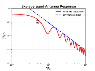
Figure 4: Sky-averaged antenna response for an L-shaped interferometer. The $1/f^{2}$ asymptotic behavior and the response first sensitivity peak are highlighted.

Numerical modeling for $\Omega_{\mathrm{GW}}$ thresholds is presented in Fig. 5, with parameters in Table. LABEL:table:parameters. As an illustration, we firstly model the threshold of a single detector with the first optical resonance at 1MHz. The broadband detection threshold, obtained by connecting the peak sensitivities of individual detectors, is also presented. A single detector can only saturate the broadband envelope within its optical bandwidth. To achieve the broadband limit, multiple detectors with combined peak sensitivities covering the entire frequency range are required. Under different parameter settings of cavity, the minimum detectable threshold of $\Omega_{\mathrm{GW,min}}$ could be estimated as follows:

$$\Omega_{\mathrm{GW,min}}^{\rm laser}(f) =1.7\times\left(\frac{10\mathrm{MW}}{P_{\mathrm{arm}}}\right)\left(\frac{\epsilon_{\mathrm{arm}}+\frac{\epsilon_{\mathrm{src}}T_{\mathrm{itm}}}{2}}{(10+\frac{100\times 0.01}{2})ppm}\right)$$ (73)

$$\times\left(\frac{10y}{T_{\mathrm{int}}}\right)^{\frac{1}{2}}\left(\frac{1\mathrm{kHz}}{\Delta f}\right)^{\frac{1}{2}}\left(\frac{f}{1\mathrm{MHz}}\right)^{5}\,.$$

When only the first optical bandwidth is utilized, due to the different antenna response, the minimum detectable threshold would be increased as:

$$\left(\Omega^{\rm laser}_{\mathrm{GW,min}}\right)^{1}(f) =3.9\times\left(\frac{10\mathrm{MW}}{P_{\mathrm{arm}}}\right)\left(\frac{\epsilon_{\mathrm{arm}}+\frac{\epsilon_{\mathrm{src}}T_{\mathrm{itm}}}{2}}{(10+\frac{100\times 0.01}{2})ppm}\right)$$ (74)

$$\times\left(\frac{10y}{T_{\mathrm{int}}}\right)^{\frac{1}{2}}\left(\frac{1\mathrm{kHz}}{\Delta f}\right)^{\frac{1}{2}}\left(\frac{f}{1\mathrm{MHz}}\right)^{5}\,.$$

Table 2: Key parameters in the numerical calculation of $\Omega_{\mathrm{GW}}$ detecting limit. Here, parameters here is largely better than the ultimate targets of third-generation gravitational wave detectors, thus it only gives a futuristic limitation for the fundamental sensitivity level.

Symbol	Description	Value	Unit
$\omega_{0}$	Laser frequency	$1.77\times 10^{15}$	Hz
$\lambda_{0}$	Laser wavelength	$1064$	nm
$P_{\mathrm{arm}}$	Circulating power inside arm cavity	10	MW
$T_{\mathrm{itm}}$	Transmissivity of ITM	0.01
$T_{\mathrm{src}}$	Transmissivity of signal recycling cavity	0.01
	(Almost entirely transmissive signal recycling mirror)
$\epsilon_{\mathrm{arm}}$	Arm loss coefficient	10	ppm
$\epsilon_{\mathrm{src}}$	Src loss coefficient	100	ppm

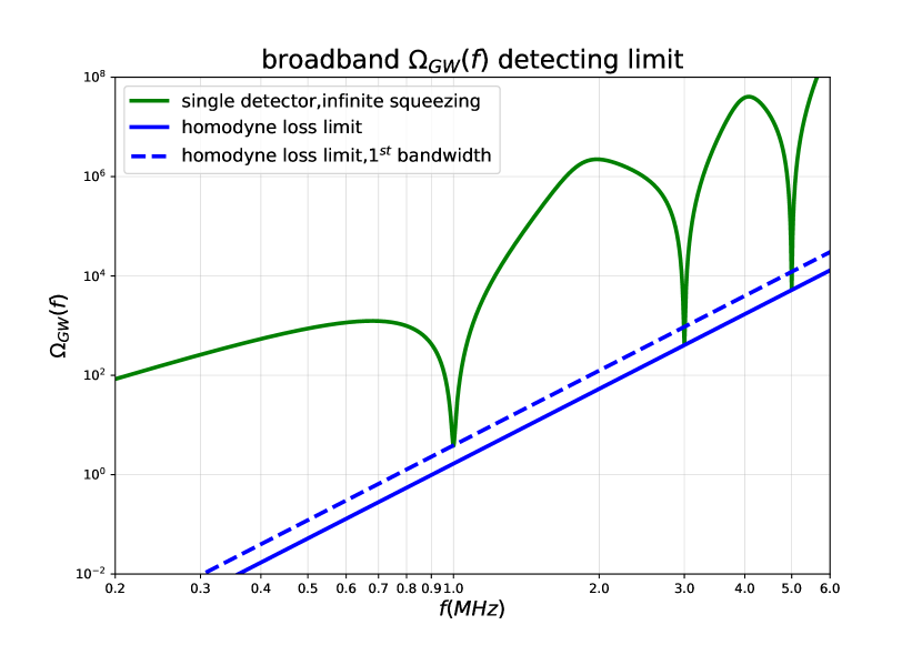
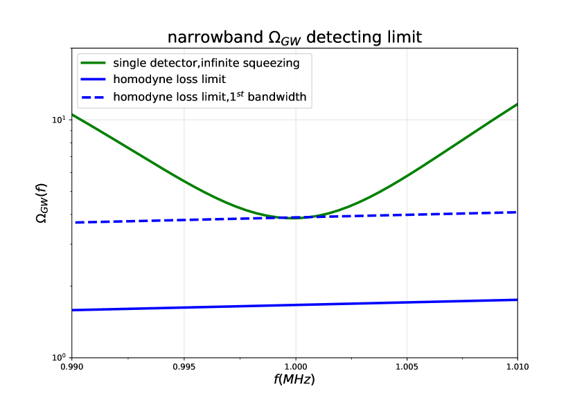
Figure 5: Broadband (upper panel) and zoomed-in (lower panel) comparisons of $\Omega_{\mathrm{GW}}$ detection limits for a single 75m L-shaped detector (homodyne readout) and a broadband detector array. Individual detectors only saturate sensitivity over narrow frequency ranges.

EM cavity: Detecting high-frequency gravitational wave signals using a resonant electromagnetic cavity is a newly proposed scheme[52]. In this proposal, the energy is stored a strong static magnetic field, and the gravitational wave signal alters the total magnetic energy stored within the cavity when it passes by. However, previous noise estimations for this proposal only accounted for readout noise, leading to an overestimation of its performance. In this section, we provide a more reliable estimation of the fundamental quantum limit for this design.

The energy stored in the system takes the form below:

$${\cal E}=\int\frac{(\vec{B_{0}}+\vec{\delta B})^{2}}{2\mu_{0}}dV\,,$$ (75)

where $\vec{B_{0}}=B_{0}\vec{e_{z}}$ is the static magnetic field in the cavity. Treating the static magnetic field as a carrier field with zero frequency and applying second quantization to the fluctuation component, this system can be effectively included in the general framework discussed in Sec. A.1.2. With only the first cavity resonant mode considered, gain in this proposal could be given by the following form:

$$|G(f)|^{2}=\frac{2\Delta\gamma\bar{\cal E}\bar{\alpha^{2}}(f)}{\hbar\cdot\left[(2\pi f-\Delta)^{2}+\gamma^{2}\right]}\,,$$ (76)

In the system, energy is stored in the static magnetic field inside the cavity, with $\bar{\cal E}=\frac{B_{0}^{2}}{2\mu_{0}}V$. $\Delta$ and $\gamma$ is the angular frequency and bandwidth of the first cavity resonant mode.

Due to the outgoing field is centered at the radio and microwave frequency bands, squeezing and photon counting are challenging to implement in this proposal. Consequently, in the modeling, we select vacuum homodyne as the readout method, with its SNR level and minimum detectable threshold given by:

$${\rm SNR}\left[\sigma^{2}\right]={\sigma^{2}}\sqrt{T_{\rm int}\Delta f}\,,$$ (77)

$$h^{2}_{\rm c,min}(f) =\frac{f}{\sqrt{T_{int}\Delta f}\cdot|G(f)|^{2}}$$ (78)

$$\Omega_{\rm GW,min} =\frac{4\pi^{2}}{3H_{0}^{2}}\frac{f^{3}}{\sqrt{T_{int}\Delta f}\cdot|G(f)|^{2}}\,.$$

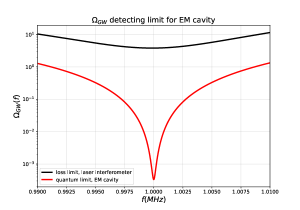
Figure 6: Quantum limit for resonant EM cavity for $\Omega_{\mathrm{GW}}$ detection. Integration time is 10 years with a frequency bin width of 1 kHz. The results show superior detection capabilities compared to a homodyne-readout laser interferometer.

As an example, we model the performance of cylindrical cavity with a height-to-radius ratio of 1:5, And the static magnetic field is set as 5T. The sensitivity peak is at the first resonant mode of cavity. At the same time, the primary restriction of the Q factor of design is Ohmic loss. Here, we set $\gamma$ as a frequency independent constant of $1k$Hz. At the same time, we estimate the sky-averaged antenna response, which is not yet well-studied, as $\bar{\alpha^{2}}(f)\sim 1$, which would not introduce order-of-magnitude difference to the fundamental limit.

To compare the detection capabilities of a single resonant EM cavity and laser interferometer, we firstly calculated the detection limit for $\Omega_{\mathrm{GW}}$ for prototypes of individual detector with peak sensitivity at 1MHz , shown in Fig. 6. We could see that, even with the absence of squeezing, the quantum limit of EM cavity still largely exceeding the loss limit of interferometer, primarily due to the large energy storage in the system. The total energy in an EM cavity with resonant frequency of $\approx 1MHz$ can reach $10^{13}$ J, significantly exceeding the $\sim 5$ J in a laser interferometer operating at the same frequency. The immense energy stored in the system actually brings a far superior energetic quantum limit to this design.

The broadband detectable threshold by combining the peak sensitivity of multiple EM cavity under different parameter setting is given by:

$$\Omega_{\mathrm{GW,min}}^{\rm cav}(f) =6.7\times 10^{-4}\times\left(\frac{5\mathrm{T}}{B_{{0}}}\right)^{2}\left(\frac{\gamma}{1kHz}\right)$$ (79)

$$\times\left(\frac{10y}{T_{\mathrm{int}}}\right)^{1/2}\left(\frac{1\mathrm{kHz}}{\Delta f}\right)^{1/2}\left(\frac{f}{1\mathrm{MHz}}\right)^{5}\,.$$

Noticing that, since ${\cal E}\propto L^{3}\propto f^{-3}$ in this proposal, size and energy is actually a big challenge for feasibility for the detection of signal at kHz range. For instance, setting the central frequency to 10 kHz would require a cavity height of approximately 30 km, along with immense energy storage. Due to technical constraints, this design remains a proof of principle at the current stage. Technically, the MHz and GHz frequency ranges are more likely to be within the scope of this proposal.

Levitating sphere: Levitating sphere is an intriguing approach for high-frequency detection[53, 54]. The basic idea is to levitate a dielectric material inside the arm cavity via optical tweezers, thus manipulating dynamical back action and enhancing sensitivity to high-frequency gravitational wave signals. Existing estimation of performance for this proposal primarily focus on thermal noise and mechanical dissipation of the dielectric object, and haven’t considered the quantum noise of electromagnetic field inside the system. Here, we provide a simple estimation of the fundamental quantum limit for the levitating sphere.

Unlike other proposals, the optical tweezer effect effectively shifts the mechanical resonance frequency in this design to our frequency range of interest, making it a system with strong mechanical back action. However, as illustrated in Sec. A.1.3 and Sec. A.2.2. In this proposal, part of the arm loss is introduced before mechanical back action, which would become the loss limit of the system. Expression of arm loss is identical to Eq. 70.

In the modeling, we set the loss rate of initial mirror and the dielectric object as both $10ppm$. For the mass of dielectric material and length or finesse of cavity, we adopt the level in [54]. Meanwhile, due to the optical tweezer effect, the arm circulating power is determined the mass of levitating object, thus cannot reach the level of laser interferometer. Under the parameter settings considered here, the circulating power is limited at $0.1W$ to $10kW$ in the frequency range we considered. Meanwhile, for order-of-magnitude estimation, the antenna response in this case is roughly estimated as $\bar{\alpha^{2}}\sim 1$.

As shown in Fig.1 in the main text, from the perspective of quantum limit, levitating sphere shows no clear advantage over traditional designs, primarily restricted by the arm circulating power. The main advantage of this design is its ability to achieve high level of squeezing. In current laser interferometers, the quantum noise is primarily restricted by the squeezing level we could achieve, a broad-band, 10dB squeezing is still not achievable yet. The strong internal squeezing in levitating sphere provides a valid solution to this technical restriction, which makes it also an alternative for future detectors.

A.3.2 Different Measurement Scheme

The rest two proposals, photon counting and channel limit, basically have physical layout of laser interferometer identical to Sec. A.3.1, but differs in the measurement scheme. We would quickly go through the modeling of these two designs.

Photon Counting: Basic principle and concept of photon counting is discussed in Sec. A.2.3. Here, we numerically study its performance in ideal condition with $\bar{\dot{n}}=0$, corresponding to the case without classical noise, dark count, and mechanical back action. In the modeling, we adopt the same configuration and optical parameters as in Sec. A.3.1. The result shows that photon counting outperforms homodyne detection for weak stochastic signals, both for single detector and broadband limit, as shown in Fig. 7. Here, the broadband sensitivity limit is also a combination of peak sensitivity of multiple detectors.

Numerically, the broadband detectable $\Omega_{\mathrm{GW}}$ threshold for ideal photon counting with different parameter settings is given by:

$$\Omega_{\mathrm{GW,min}}^{\rm pc}(f) =2.8\times 10^{-3}\times\left(\frac{10\mathrm{MW}}{P_{\mathrm{arm}}}\right)\left(\frac{T_{\mathrm{src}}}{0.01}\right)$$ (80)

$$\times\left(\frac{10y}{T_{\mathrm{int}}}\right)\left(\frac{1\mathrm{kHz}}{\Delta f}\right)\left(\frac{f}{1\mathrm{MHz}}\right)^{5}.$$

If only the first optical bandwidth is utilized, the corresponding detection limit becomes:

$$\left(\Omega_{\mathrm{GW,min}}^{\rm pc}\right)^{1}(f) =6.6\times 10^{-3}\times\left(\frac{10\mathrm{MW}}{P_{\mathrm{arm}}}\right)\left(\frac{T_{\mathrm{src}}}{0.01}\right)$$ (81)

$$\times\left(\frac{10y}{T_{\mathrm{int}}}\right)\left(\frac{1\mathrm{kHz}}{\Delta f}\right)\left(\frac{f}{1\mathrm{MHz}}\right)^{5}.$$

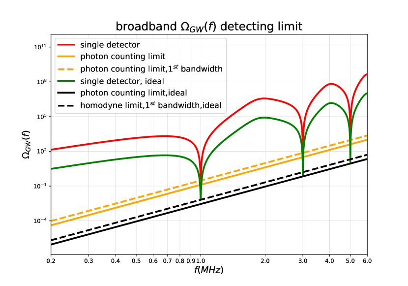
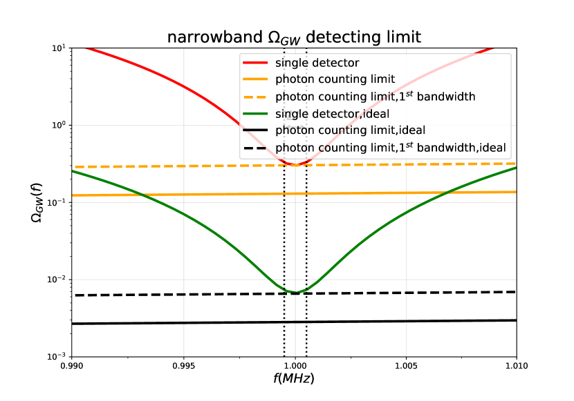
Figure 7: Broadband(upper panel) and zoomed-in(lower panel) comparison of the $\Omega_{\mathrm{GW}}$ detection limit of a single 75m L-shaped detector against the broadband detection $\Omega_{\mathrm{GW}}$ limit of a detector array, with both homodyne detection and photon counting . The effective detection bandwidth is defined as the region between the two vertical black dotted lines.

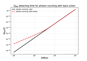
Figure 8: $\Omega_{\rm GW}$ limit for photon counting with and without mechanical back action, where $T_{\rm int}=10y$ and $\Delta f=1k$Hz. Basically, mechanical back action will not largely affects the fundamental quantum limit at ultra-high frequency.

We also study the influence of mechanical back action to the minimum detectable threshold. In a laser interferometer, the strength of mechanical back action can be quantitatively described by a parameter $\cal K$, defined as:

$${\cal K}^{2}(f)=\frac{S^{\rm vac}_{\rm rad}(f)}{S^{\rm vac}_{\rm shot}(f)}\,,$$ (82)

where $S^{\rm vac}_{\rm shot}(f)$ and $S^{\rm vac}_{\rm rad}(f)$ is the quantum shot noise level and quantum radiation noise level with vacuum state injection. Back-action would lead to an additional photon flux at readout, given by:

$$\bar{\dot{n}}\approx\frac{{\cal K}^{2}}{4}\cdot{\Delta f}\,.$$ (83)

Applying Eq. 65, the minimum detectable threshold for unity SNR with back action takes the following form:

$$\Omega^{\rm pc}_{\rm GW,min}(f)=\frac{4\pi^{2}}{3H_{0}^{2}}\frac{f^{3}\left(1+\sqrt{1+{\cal K}^{2}T_{\rm int}/\Delta f}\right)}{T_{\rm int}\Delta fS^{\rm vac}_{\cal EE}(f)\bar{\alpha^{2}}(f)}\,.$$ (84)

In L-shaped interferometer, the coefficient $\cal K$ can be expressed in terms of the detector parameters as[11]:

$${\cal K}(f)=\frac{32\omega_{0}P_{\rm arm}}{(2\pi f)^{2}\cdot Mc^{2}T_{\rm src}}\,,$$ (85)

where $M$ is the mass of end mirror, and optical parameters are defined in Tab. LABEL:table:parameters. By setting the mass of the end mirror to 500 kg, we numerically model the impact of mechanical back action, as presented in Fig. 8. With this parameter setting, the back action only destroys the $1/f^{5}$ scaling of $\Omega_{\rm GW}$ limit below 3kHz. At ultra-high frequencies, back action does not significantly affect the system’s performance. Thus, feasibility of photon counting is basically restricted by classical effects, like the classical noise or the dark count (false reading at the single-photon detector).

Channel Limit: As discussed in Sec. A.2.4, the channel limit is actually the ultimate sensitivity limit over all the possible input quantum state and readout scheme, and specific measurement scheme that saturates the channel limit remains largely uncertain. Numerical value for minimum detectable threshold for $h_{c}^{2}$ and $\Omega_{\rm GW}$ for channel limit are simply ${\epsilon}$ times of that of ideal photon counting, with the same loss rate as interferometer with linear measurement.

It is conceivable that, due to the use of entangled and non-Gaussian states, implementation of concrete design that saturates the bound would be even more challenging compared to linear readout and photon counting. The loss-limited behavior highlights the extensive manipulation required for the input quantum state, posing challenges for state preparation. Similarly, the ideal performance with zero noise in the absence of a signal implies that the corresponding quantum state and measurement would be highly sensitive to intrinsic parameters, such as ancilla loss and internal squeezing. Consequently, the the detection scheme corresponding to the channel limit is highly futuristic. Nonetheless, as the ultimate limit for a broad class of laser interferometer-based proposals, it is still important in guiding and constraining future designs.

Appendix B Cosmological phase transitions motivated by GUTs

B.1 Review of Phase Transition and Gravitational Wave

There are three main contributions to the production of phase transition gravitational wave which are denoted as bubble shell collision, sound wave as well as turbulence. In most of the cases, however, the sound wave contributions will be dominant. The bubble shell collision will be important in cases when supercooling occurs. The expression for the acoustic gravitational wave power spectrum today is[25]:

$$h^{2}\Omega_{\text{GW}}(f)=2.061h^{2}F_{\rm{gw,0}}\Gamma^{2}\bar{U}_{f}^{4}\left(H_{n}R_{*}\right)\tilde{\Omega}_{\rm{gw}}S_{\text{sw}}(f/f_{p})\,,$$ (86)

where

$$F_{\rm{gw,0}}=3.57\times 10^{-5}\left(\frac{100}{g_{*}}\right)^{\frac{1}{3}}\,,$$ (87)

which is a transformation factor that connects the GW energy density at the time of its production to the GW energy density observed today. $\bar{U}_{f}$ is the root-mean-square (RMS) fluid velocity and $\Gamma=1+\bar{p}/\bar{\epsilon}=4/3$ is the adiabatic index derived from the enthalpy density and is associated with the fluid source tensor (we have used $\bar{p}=1/3\bar{\epsilon}$ during the radiation period). By definition, we have:

$$\Gamma\,\bar{U}_{f}^{2}=\frac{\kappa_{v}\alpha}{1+\alpha}\qquad\left({\rm{or}}\,\,\bar{U}_{f}^{2}=\frac{3}{4}\frac{\kappa_{v}\alpha}{1+\alpha}\right)\,,$$ (88)

where $\kappa_{v}$ is the efficiency factor which will be discussed in more details below while $\alpha$ is the phase transition strength parameter defined using trace anomaly (see e.g. [55]). $\tilde{\Omega}_{\rm{gw}}$ is the dimensionless gravitational wave energy density which is approximately constant and is around $1.2\times 10^{-2}$. Note that the value of $\tilde{\Omega}_{\rm{gw}}$ is much smaller, when the bubble wall velocity is closed to the Chapman-Jouguet velocity (sound wave velocity). This is because, when the bubble wall velocity approaches the sound speed, the thickness of the sound shell vanishes, suppressing the gravitational waves generated by sound waves. On the other hand $H_{n}$ denotes the Hubble constant at the bubble nucleation while $R_{*}$ is the mean bubble separation. We have:

$$H_{n}R_{*}=\left(8\pi\right)^{1/3}\frac{v_{w}H_{n}}{\beta}=\left(8\pi\right)^{1/3}\frac{v_{w}}{\tilde{\beta}}\,,$$ (89)

where the last step, we have used $\tilde{\beta}\equiv\beta/H$. For the $\rm{h}^{2}$ denotes the reduced Hubble constant square, we can implement the current Planck best-fit value ${\rm{h}}=0.678$. Finally, $S_{\text{sw}}(f/f_{p})$ represents the shape factor which determines the form of the gravitational wave power spectrum around its peak. By using the simulation plus fitting, it reads[25]:

$$S_{\text{sw}}(f/f_{p})=\left[\frac{4}{7}+\frac{3}{7}\left(\frac{f}{f_{\text{peak}}}\right)^{\!2}\right]^{-\frac{7}{2}}\,.$$ (90)

It can be shown easily that in the high frequency limit $S_{\rm{sw}}\propto f^{-4}$ while in the low frequency limit $S_{\rm{sw}}\propto f^{3}$ which is consistent with the simulation. If we combine all the above factors together, the GW spectrum from sound waves reads:

$${\rm{h}}^{2}\Omega_{\text{GW}}(f) ={\rm{h}}^{2}\Omega^{\text{peak}}_{\text{GW}}\left(\frac{f}{f_{\text{peak}}}\right)^{\!3}\left[\frac{4}{7}+\frac{3}{7}\left(\frac{f}{f_{\text{peak}}}\right)^{\!2}\right]^{-\frac{7}{2}},$$ (91)

with the peak frequency

$$f_{\text{peak}} \simeq 8.9\cdot 10^{-6}\,\text{Hz}\left(\frac{g_{*}}{100}\right)^{\!\frac{1}{6}}\left(\frac{T}{100\,\text{GeV}}\right)\left(\frac{\tilde{\beta}}{v_{w}}\right),$$ (92)

and the peak amplitude

$${\rm{h}}^{2}\Omega^{\text{peak}}_{\text{GW}} \simeq 1.19\cdot 10^{-6}\left(\frac{v_{w}}{\tilde{\beta}}\right)\left(\frac{\kappa_{\rm{sw}}\,\alpha}{1+\alpha}\right)^{\!2}\left(\frac{100}{g_{*}}\right)^{\!\frac{1}{3}}\,.$$ (93)

We discuss the two key parameters the inverse duration $\beta$ and the strength $\alpha$ of the phase transition respectively below. For inverse duration $\beta$, with sufficiently fast phase transitions, the decay rate can be approximated by

$$\Gamma(T)\approx\Gamma(t_{*})e^{\beta(t-t_{*})}\,,$$ (94)

where $t_{*}$ is the characteristic time scale for the production of GWs. The inverse duration time then follows as

$$\beta=-\frac{\mathrm{d}}{\mathrm{d}t}\frac{S_{3}(T)}{T}\bigg{|}_{t=t_{*}}\,.$$ (95)

The dimensionless version is obtained by dividing with the Hubble parameter $H$

$$\tilde{\beta}=\frac{\beta}{H_{*}}=T\frac{\mathrm{d}}{\mathrm{d}T}\frac{S_{3}(T)}{T}\bigg{|}_{T=T_{*}}\,,$$ (96)

where we used that $\mathrm{d}T/\mathrm{d}t=-H(T)T$.

On the other hand, the strength parameter $\alpha$ can be defined by using the trace of the energy-momentum tensor $\theta$

$$\alpha=\frac{1}{3}\frac{\Delta\theta}{w_{+}}=\frac{1}{3}\frac{\Delta e\,-\,3\Delta p}{w_{+}}\,,$$ (97)

where $\Delta X=X^{(+)}-X^{(-)}$ for $X=(\theta$, $e$, $p$) and $(+)$ denotes the meta-stable phase (outside of the bubble) while $(-)$ denotes the stable phase (inside of the bubble). The enthalpy density $w_{\pm}$ is defined by

$$w_{\pm}=\frac{\partial p}{\partial\ln T}\bigg{|}_{\pm}\,,$$ (98)

which encodes the information of the number of relativistic degrees of freedom (d.o.f). It is intuitive to use the trace of the energy momentum tensor $\theta$ to quantify the strength of the phase transition $\alpha$. In the limiting case when $\theta=0$, the system possesses conformal symmetry and there is a smooth second-order phase transition occurring.

The last important ingredient is the total efficiency factor $\kappa_{\rm{sw}}$, which describes the fraction of energy that is used to produce GWs. The total efficiency factor is made up of the efficiency factor $\kappa_{v}$ [27] and an additional suppression factor due to the length of the sound-wave period [56, 57, 28]. In total, the efficiency factor $\kappa_{\text{sw}}$ is given by

$$\kappa_{\text{sw}} =\sqrt{\tau_{\text{sw}}}\,\kappa_{v}\,.$$ (99)

For $v_{w}=1$, $\kappa_{v}$ is given by

$$\kappa_{v}(v_{w}=1)=\frac{\alpha}{0.73+0.083\sqrt{\alpha}+\alpha}\,,$$ (100)

which implies $\kappa_{v}\approx 0.3$ for $\alpha\approx 1/3$. At the Chapman-Jouguet detonation velocity $v_{J}$, the efficiency factor reads

$$\kappa_{v}(v_{w}=v_{J})=\frac{\sqrt{\alpha}}{0.135+\sqrt{0.98+\alpha}}\,,$$ (101)

and for $\alpha\approx 1/3$ we have $\kappa_{v}\approx 0.45$. As expected, this value is larger that for $v_{w}=1$. For smaller wall velocities $v_{w}<c_{s}$, where $c_{s}=1/\sqrt{3}$ is the speed of sound, the efficiency factor decreases rapidly and the generation of GW from sound waves is suppressed [58].

The factor $\tau_{\rm{SW}}$ has been analyzed in details in recent work [28]. They analysed the length of the sound-wave period in an expanding universe and is given by:

$$\tau_{\text{sw}}=1-1/\sqrt{1+2\frac{(8\pi)^{\frac{1}{3}}v_{w}}{\tilde{\beta}\,\bar{U}_{f}}}\,.$$ (102)

The above factor provides an additional suppression of the sound wave generated gravitational wave signals if the inverse duration $\tilde{\beta}$ is large.

B.2 Review of SO(10) GUT breaking

There are various ways to achieve the breaking from $SO(10)$ to the SM gauge group. Each “breaking chain” has a distinct pattern of intermediate gauge symmetries and we use the following abbreviations for these gauge groups:

$$G_{51} =SU(5)\times U(1)_{\chi}\,,$$

$$G_{51}^{\rm flip} =SU(5)^{\rm flip}\times U(1)_{V}\,,$$

$$G_{422} =SU(4)_{c}\times SU(2)_{L}\times SU(2)_{R}\,,$$

$$G_{421} =SU(4)_{c}\times SU(2)_{L}\times U(1)_{R}\,,$$

$$G_{3221} =SU(3)_{c}\times SU(2)_{L}\times SU(2)_{R}\times U(1)_{X}\,,$$

$$G_{3211} =SU(3)_{c}\times SU(2)_{L}\times U(1)_{Y}\times U(1)_{B-L}\,,$$

$$G_{\rm SM} =SU(3)_{c}\times SU(2)_{L}\times U(1)_{Y}\,.$$ (103)

Here, $SU(5)$ represents the usual Georgi-Glashow group, $SU(5)^{\rm flip}\times U(1)_{V}$ is the gauge group in flipped $SU(5)$ model, in which the up-type quarks and down-types quarks, as well as neutrinos and charged leptons, are flipped in their representations compared with those in the Georgi-Glashow $SU(5)$. $G_{422}$ is the Pati-Salam gauge group, where leptons are treated as the fourth colour of quarks. $SO(10)$ includes an intrinsic $Z_{2}^{C}$ parity symmetry between left chiral field and the charge conjugate of the right chiral field. It might keep unbroken during $SO(10)$ breaking to $G_{422}$. In the Pati-Salam model, this $Z_{2}^{C}$ appears as the permutation symmetry between matter fields $(\overline{{\bf 4}},{\bf 2},{\bf 1})$ and $({\bf 4},{\bf 1},{\bf 2})$. We abbreviate the Pati-Salam gauge group preserving $Z_{2}^{C}$ as $G_{422}^{C}\equiv G_{422}\times Z_{2}^{C}$. This $Z_{2}^{C}$ may be still preserved for the breaking from $G_{422}$ to $G_{3221}$, and we denote the latter case as $G_{3221}^{C}\equiv G_{3221}\times Z_{2}^{C}$. Note that in some notation, the $G_{3211}$ is considered to be $SU(3)_{c}\times SU(2)_{L}\times U(1)_{R}\times U(1)_{X}$. It is equivalent to represent as $U(1)_{Y}\times U(1)_{B-L}$ as the former two $U(1)$ charges are just a mixing of the later two, i.e., $\pm R=Y-\frac{B-L}{2}$ and $X=\sqrt{\frac{3}{2}}\frac{B-L}{2}$, where the $\pm$ signs refer to two mays of embedding $G_{3211}$ in $G_{51}$ and $G_{51}^{\rm flip}$.

All breaking chains from $SO(10)$ to $G_{\rm SM}$ are presented in Fig. 2 in the main text, which can be classified into four categories [59] and also presented below. Each breaking chain leads to topological defects generated in the early Universe. We will check, from chain to chain, if a SGWB signal is observable via a cosmological phase transition via a GUT-related intermediate symmetry breaking, mainly focusing on the breaking of the lowest intermediate symmetry breaking to the SM gauge symmetry.

• The breaking chain with the Georgi-Glashow $SU(5)$ and the $U(1)_{B-L}$ as an intermediate symmetry.

  $$SO(10)\mathrel{\mathop{\hbox{}\longrightarrow}\limits^{\rm m}}G_{51}\mathrel{\mathop{\hbox{}\longrightarrow}\limits^{\rm m}}G_{3211}\mathrel{\mathop{\hbox{}\longrightarrow}\limits^{\rm s}}G_{\rm SM}$$

  The breaking of $SO(10)\to G_{51}$ and $G_{51}\to G_{3211}$ (which is essentially $SU(5)\to G_{\rm SM}$) generates monopoles, which are denoted by “m” above the arrow. The null observation of proton decay requires the BNV breaking scale, as well as the corresponding monopole mass generated at the same scale, above $10^{15}$ GeV. These super heavy monopoles will dominate the energy density of the Universe later during the expansion and thus they are unwanted topological defects and should be inflated. The breaking $G_{3211}\to G_{\rm SM}$ (which is essentially the breaking of the gauge $U(1)_{B-L}$) generates cosmic strings, denoted as “s” above the arrow. As the existence of cosmic strings is safe for the evolution of Universe in the radiation- and matter-domination eras, the inflation can be introduced before the breaking of $G_{3211}$. In other word, we can assume reheating processes before the breaking of $G_{3211}$. As a consequence, the phase transition for $U_{B-L}$ breaking and the generation of cosmic strings happens in the radiation era. In this breaking chain, there is no restriction on the breaking scale of $U(1)_{B-L}$ as it is separated from the $SU(5)$ unification. For a SGWB spectrum with the peak frequency around kHz - MHz, the $U(1)_{B-L}$ breaking scale should be somewhere within $10^{6}$ - $10^{9}$ GeV.

• The breaking chain with the flipped $SU(5)\times U(1)$ as intermediate symmetry.

  $$SO(10)\mathrel{\mathop{\hbox{}\longrightarrow}\limits^{\rm m}}G_{51}^{\rm flip}\mathrel{\mathop{\hbox{}\longrightarrow}\limits^{\rm s}}G_{\rm SM}$$

  In this chain, the breaking of $G_{51}^{\rm flip}\to G_{\rm SM}$ produces cosmic strings which are safe for the cosmological evolution. However, the breaking scale should be $\gtrsim 10^{15}$ GeV to satisfy the proton decay constraint. If a SGWB is generated via phase transition, the frequency will be super-high with the peak frequency roughly around $10^{15}$ Hz. This is impossible to be observed in the future GW measurements.

• Breaking chains with the Pati-Salam symmetry $G_{422}$ or its subgroups as intermediate symmetries. This category provides the largest possibility with 31 different chains in total [23]. They can be further sorted within two types.

  $$(\text{c}_{1}) \quad SO(10)\to...\to G_{421},G_{3221},G_{3211}\mathrel{\mathop{\hbox{}\longrightarrow}\limits^{\rm s}}G_{\rm SM}$$

  $$(\text{c}_{2}) \quad SO(10)\to...\to G_{422}\mathrel{\mathop{\hbox{}\longrightarrow}\limits^{\rm m,(s)}}G_{\rm SM}$$

  $$(\text{c}_{3}) \quad SO(10)\to...\to G_{422}^{C},G_{3221}^{C}\mathrel{\mathop{\hbox{}\longrightarrow}\limits^{\rm w,(s,m)}}G_{\rm SM}$$ (104)

  In (c₁), the breaking of the last intermediate symmetry to $G_{\rm SM}$, e.g., $G_{3221}\to G_{\rm SM}$, generates only cosmic strings. Thus, inflation can be introduced before it. As a consequence, a cosmological phase transition of the last intermediate symmetry happens during the radiation era. In (c₂), the breaking of the last intermediate symmetry to $G_{\rm SM}$, e.g., $G_{422}\to G_{\rm SM}$, generates monopoles, where strings may be generated but domain walls are not. In (c₃), the breaking of the last intermediate symmetry to $G_{\rm SM}$ generates domain walls, denoted as “w” above the arrow. Most breaking chains (26 of 31) belong to type (c₁) and only 2 chain and 3 chains belongs types (c₂) and (c₃), respectively [23]. For type (c₁) chains, similar to chains in category (a), inflation can be introduced before the breaking of the lowest intermediate symmetry, and thus the SGWB from the phase transition, if it is first-order, might be observed. Note that, here the phase transition could happen along with $G_{3221}\to G_{\rm SM}$ or $G_{421}\to G_{\rm SM}$, which are essentially the breaking of $SU(2)_{R}\times U(1)_{X}\to U(1)_{Y}$ and $SU(4)_{c}\times U(1)_{R}\to SU(3)_{c}\times U(1)_{Y}$, respectively. More DOF of gauge bosons, as well as necessary Higgs multiplets responsible for the symmetry breaking, helps to promote the phase transition to be first-order. Following the discussions in e.g., [60, 61, 23], the energy scale of the lowest intermediate symmetry breaking span several orders of magnitude. It could be as high as $10^{13}$ GeV, or decrease to $10^{6}$ GeV, depending on the breaking chains, particle contents included in the RG running for the gauge unification. In this work, we will take care those might be observable in kHz - MHz GW measurements, referring to the energy scale around $10^{6}$ - $10^{9}$ GeV. In type (c₂), monopoles are generated, and their masses are naturally around the same scale of the symmetry breaking, i.e., in our preset regime $\sim 10^{6}$ - $10^{9}$ GeV. They are too light to dominate the energy density of the expanding Universe, and thus inflation does not have to be introduced after their production [62, 63]. In type (c₃), domain walls are generated due to the spontaneous breaking of $Z_{2}^{C}$. Any topologically stable domain walls with the mass scale above 10 MeV generated after inflation can overclose the Universe [39] and thus type (c₃) will not be considered.

• Breaking chains with the standard $SU(5)$ subgroup as the lowest intermediate scale before breaking to $G_{\rm SM}$,

  $$SO(10)\to...\to SU(5)\mathrel{\mathop{\hbox{}\longrightarrow}\limits^{\rm m}}G_{\rm SM}$$

  These chains have the last intermediate symmetry as the Georgi-Glashow $SU(5)$. The null observation of proton decay requires the $SU(5)$ scale above $10^{15}$ GeV. It is well-known that the breaking of $SU(5)$ at such a high scale leads to the monopole problem. Thus, inflation is necessary after the symmetry breaking.

We have checked that most breaking chains, (a, c₁, c₂), in the $SO(10)$ framework give the possibility of a cosmological phase transition which is sufficiently higher the electroweak scale. They do not encounter the cosmological problem which has to be solved via the introduction of inflation. GWs via cosmological phase transition in the radiation era might be observable for any of these chains.

For some of chains (c₁), the breaking of the second lowest intermediate symmetry to the lowest intermediate symmetry generates monopoles. We list them below,

$$SO(10)\to...\to G_{422}\mathrel{\mathop{\hbox{}\longrightarrow}\limits^{\rm m}}G_{421},G_{3221},G_{3211}\mathrel{\mathop{\hbox{}\longrightarrow}\limits^{\rm s}}G_{\rm SM}$$

$$SO(10)\to...\to G_{421},G_{3221}\mathrel{\mathop{\hbox{}\longrightarrow}\limits^{\rm m}}G_{3211}\mathrel{\mathop{\hbox{}\longrightarrow}\limits^{\rm s}}G_{\rm SM}$$ (105)

If the scale of the second lowest intermediate scale and the consequent monopole mass are in the preset regime as suggested in the above, there will be no cosmological problem for it, and we can further consider the phase transition via these breakings.

In conclusion, the SO(10) GUT framework provides rich possibilities for cosmological phase transition with scale in the regime $10^{6}$ - $10^{9}$ GeV in the radiation era. Depending on the breaking chains, and the large DOF from new particle contents evolving in the phase transition, the phase transition can be first order and generate sizeable GW signals. We will further study the phase transition in the next subsection.

B.3 Phase transition motivated by GUTs

By assuming the gauge symmetry as some intermediate symmetries as discussed in the last section, we further cosmological phase transition referring to the spontaneous breaking of these symmetries. In particular, we will focus on the simplification of the effective potential and the calculation of $\alpha$ and $\tilde{\beta}$, which are key parameters for observable GWs. In this simplified treatment, we will see how the key parameters in phase transition and GW production are determined by physical parameters (e.g., Higgs vecuum expectation value, masses of heavy particles) in a particle theory.

Given the gauge symmetry breaking $G_{M}\to G_{n}$ with $G_{n}$ as a subgroup of $G_{M}$ (typically for example $G_{422}\to G_{3221}$ or $G_{3221}\to G_{\rm SM}$), we assume the symmetry breaking is achieved by a Higgs mechanism via a single scalar field $\phi$ gaining a non-zero VEV. In detail, the theory includes a scalar component $\phi$, which belongs to a Higgs multiplet of $G_{M}$ and itself is a trivial singlet of $G_{n}$. Once it gains the VEV, $G_{M}$ is spontaneously broken and $G_{n}$ is left as a remnant symmetry.

Without loss of generality, we regard $\phi$ is real and positive, and we can write out the effective potential of $\phi$ during the symmetry breaking. Note that at the scale much higher than the electroweak scale, the SM Higgs is staying in the EW-symmetric vacuum and its field value is fixed at zero. Thus, it does not contribute to the phase transition here directly. By treating $\phi$ as a classical field, the effective potential of $\phi$ is written to be

$$V_{\rm eff}^{T}(\phi)=V_{0}(\phi)+V_{1}^{0}(\phi)+V_{1}^{T}(\phi)\,.$$ (106)

Here $V_{0}(\phi)$ refers to the tree-level potential of $\phi$, $V^{0}_{1}(\phi)$ is reduced from the one-loop Coleman-Weinberg correction at zero temperature, and the finite-temperature corrections is included in $V_{1}^{T}(\phi)$. They are respectively written out to be

$$V_{0}(\phi) =\frac{M_{\phi}^{2}}{8v_{\phi}^{2}}(\phi^{2}-v_{\phi}^{2})^{2}\,,$$

$$V^{0}_{1}(\phi) =\frac{1}{64\pi^{2}}\,\Big{[}\sum_{b}\,g_{b}G_{b}(\phi)-\sum_{\psi}\,g_{f}G_{\psi}(\phi)\Big{]}\,,$$

$$V^{T}_{1}(\phi) =\frac{T^{4}}{2\pi^{2}}\Big{[}\sum_{b}\,g_{b}J_{b}(\phi)-\sum_{f}\,g_{f}J_{f}(\phi)\Big{]}+V^{T}_{\rm daisy}(\phi)\,,$$ (107)

where $b$ and $f$ run for relevant bosonic and fermionic contributions, respectively, and $g_{b}$ and $g_{f}$ refer to the effective DOF of each particle contributing to the process. In the Coleman-Weinberg correction, $G_{i}(\phi)$ for either bosonic or fermionic correction is written in a unified form using the on-shell regularisation

$$G_{i}(\phi) ={\bf m}_{i}^{4}(\phi)\left[\log\frac{{\bf m}^{2}_{i}(\phi)}{M_{i}^{2}}-{\frac{3}{2}}\right]+2\,{\bf m}_{i}^{2}(\phi)\,M_{i}^{2}\,.$$ (108)

${\bf m}_{i}(\phi)$ is the field-dependent mass for particle $i$ during the phase transition. During the phase transition, particle gains the mass. We consider the single field phase transition and then ${\bf m}_{i}(\phi)$, for all relevant particles except $s$, takes the same form ${\bf m}^{2}_{i}(\phi)=M_{i}^{2}\phi^{2}/v_{\phi}^{2}$. As for the Higgs $\phi$,

$${\bf m}_{\phi}^{2}(\phi) =-\mu_{\phi}^{2}+3\lambda_{\phi}\phi^{2}=\frac{M_{\phi}^{2}}{2}\big{(}\frac{3\phi^{2}}{v_{\phi}^{2}}-1\big{)}\,,$$ (109)

In the thermal correction $V_{1}^{T}(\phi)$,

$$J_{b}(\phi) =\int_{0}^{\infty}dy\,y^{2}\,\log\left[1-\exp\big{(}-\sqrt{{\bf m}_{b}^{2}(\phi)/T^{2}+y^{2}}\big{)}\right]\,,$$

$$J_{f}(\phi) =\int_{0}^{\infty}dy\,y^{2}\,\log\left[1+\exp\big{(}-\sqrt{{\bf m}_{f}^{2}(\phi)/T^{2}+y^{2}}\big{)}\right]\,,$$

$$V^{T}_{\rm daisy}(\phi) =-\frac{T}{12\pi}\sum_{b^{\prime}}\,g_{b^{\prime}}\left\{[{\bf m}_{b}^{2}(\phi)+\Pi_{b^{\prime}}]^{3/2}-[{\bf m}_{b^{\prime}}^{2}(\phi)]^{3/2}\right\}\,,$$ (110)

Here $b$ and $f$ runs for all bosonic and fermionic contributions, respectively and $b^{\prime}$ running for scalar and longitudinal contributions. The daisy contribution is included following the Arnold-Espinosa approach [64]. The finite-temperature contribution can be expanded in terms of $x_{b,f}\equiv{\bf m}_{b,f}^{2}(\phi)/T^{2}$ as [65, 66],

$$J_{b}(\phi) =-\frac{\pi^{4}}{45}+\frac{\pi^{2}}{12}x_{b}-\frac{\pi}{6}x_{b}^{3/2}-\frac{1}{32}x_{b}^{2}\,\log{\frac{x_{b}}{a_{B}}}+\cdots\,,$$

$$J_{f}(\phi) =\frac{7\pi^{4}}{360}-\frac{\pi^{2}}{24}x_{f}-\frac{1}{32}x_{f}^{2}\,\log\frac{x_{f}}{a_{F}}+\cdots\,,$$ (111)

where $a_{b}=16\,\pi^{2}\,\exp(3/2-2\gamma_{E})$, $a_{f}=\pi^{2}\exp(3/2-2\gamma_{E})$, with $\gamma_{E}=0.5772$, and the dots denote the higher order terms. In the regime ${\bf m}_{b}^{2}(x)<5T^{2}$ and ${\bf m}_{f}^{2}(x)<3T^{2}$, the dots terms lead to deviation less than $5\%$ [67]. We will restrict our discussion in this regime and thus the dots terms can be safely ignored. With the above treatment, we will be able to re-write the effective potential approximately in the form of a polynomial of $\phi$,

$$V_{\rm eff}(\phi)\approx D(T^{2}-T_{0}^{2})\phi^{2}-AT\phi^{3}+\frac{\lambda_{T}}{4}\phi^{4}\,.$$ (112)

Here, the parameters $D$, $T_{0}$, $A$ and $\lambda_{T}$ respect to GUT intermediate symmetries are the parametrisation below

$$D =\frac{M_{\phi}^{2}}{16v_{\phi}^{2}}+\frac{p}{24}\,,$$

$$T_{0} =\sqrt{\Big{(}\frac{1}{4}M_{\phi}^{2}-\frac{qv_{\phi}^{2}}{32\pi^{2}}\Big{)}/D}\,,$$

$$\lambda_{T} =\frac{M_{\phi}^{2}}{2v_{\phi}^{2}}+\frac{q}{16\pi^{2}}\Big{(}1+\log\frac{T^{2}}{rv_{\phi}^{2}}\Big{)}\,,$$

$$A ={\frac{a}{12\pi}}+\delta A\,.$$ (113)

with

$$p =\frac{1}{v_{\phi}^{2}}\Big{(}\sum_{S}M_{S}^{2}+3\sum_{G}M_{G}^{2}+\sum_{F}M_{F}^{2}\Big{)}\,,$$

$$q =\frac{1}{v_{\phi}^{4}}\Big{(}\sum_{S}M_{S}^{4}+3\sum_{G}M_{G}^{4}-2\sum_{F}M_{F}^{4}\Big{)}\,,$$

$$r =\exp\Big{[}1-\frac{1}{qv_{\phi}^{4}}\Big{(}\sum_{S}f_{S}^{T}M_{S}^{4}+3\sum_{G}f_{G}^{T}M_{G}^{4}$$

$$-2\sum_{F}f_{F}^{T}M_{F}^{4}\Big{)}\Big{|}_{T=v_{\phi}}\Big{]}\,,$$

$$a =\frac{2}{v_{\phi}^{3}}\sum_{G}M_{G}^{3}$$ (114)

where the subscripts $S$, $G$, $F$ sum for extra relevant scalar except the Higgs $\phi$, gauge bosons and fermions, respectively. $\lambda_{T}$ is slightly $T$-dependent due to the $\log T$ terms from the loop correction. We have ignored the $\log T$-dependent term contributed from the scalar $S$, as it is subleading compared with its tree-level contribution. In the formula of $A$, the first term is the thermal correction induced by the transverse components of gauge bosons. $\delta A$ accounts for additional contributions from scalar or longitudinal vector, which may not be fully screened. We ignore it for simplicity. $f_{S}^{T}=\log\frac{{A_{B}}T^{2}}{M_{S}^{2}}$, $f_{G}^{T}=\log\frac{{A_{B}}T^{2}}{M_{G}^{2}}$ and $f_{f}^{T}=\log\frac{{A_{F}}T^{2}}{M_{f}^{2}}$ with $A_{B}=A_{b}e^{-3/2}$ and $A_{F}=a_{F}e^{-3/2}$.

Given polynomial potential in the form of Eq. (112), we can calculate the key parameters $\alpha$ and $\tilde{\beta}$ analytically with the help of the following parameterisation. We re-write the potential in the form $V=N\widetilde{V}(\widetilde{\phi})$ with the normalised and dimensionless potential

$$\widetilde{V}(\widetilde{\phi})=\frac{\widetilde{\phi}^{2}\left(\widetilde{\phi}^{2}-4\widetilde{\phi}{+}4bz\right)}{4(1-z)^{2}}$$ (115)

where

$$\widetilde{\phi}=\sqrt{1-z}\frac{\lambda_{T}\phi}{AT_{0}}\,.$$ (116)

Here, we have introduced one $T$-dependent viable and two $T$-insensitive factors

$$z=1-\frac{T_{0}^{2}}{T^{2}}\,;\quad b=\frac{\lambda_{T}D}{A^{2}}\,,\quad N=\frac{A^{4}T_{0}^{4}}{\lambda_{T}^{3}}\,.$$ (117)

The potential has two local minima and one local maxima at

$$\widetilde{\phi}=0,(3+\sqrt{9-8bz})/2,\text{ and }(3-\sqrt{9-8bz})/2\,,$$ (118)

respectively. For $z=1/b$, the two local minima become degenerate, and this corresponds to the system at the critical temperature $T_{c}$. We denote the value of $z$ at the phase transition by $z_{\star}$. Since $T_{0}<T_{\star}<T_{c}$, respectively, $z_{\star}$ is restricted as

$$0<z_{\star}\equiv 1-\frac{T_{0}^{2}}{T_{\star}^{2}}<\frac{1}{b}<1\,.$$ (119)

Here the requirement $b>1$ is to ensure the two local minima to flip at some point for temperature dropping from a sufficiently high scale to $T_{0}$.

The 3D action in the parametrisation can be semi-analytically written as

$$\frac{S_{3}(T)}{T}=\frac{D^{3/2}}{A^{2}}z^{3/2}f\left(bz\right)$$ (120)

where the function $f(x)$ is semi-analytically given by

$$f(x)\simeq 4.85\times\left[1+\frac{x}{4}\left(1+\frac{2.4}{1-x}+\frac{0.26}{(1-x)^{2}}\right)\right]$$ (121)

With the above parametrisation, we are able to derive analytical expressions for the key parameters $\tilde{\beta}$ and $\alpha$ for GW production. We remind these parameters are defined in Eq. (97) at the percolation temperature $T_{\star}$. $\Delta\theta$ in our particular case is simplified into

$$\Delta\theta=\Delta V-\frac{T}{4}\frac{\partial\Delta V}{\partial T}\,.$$ (122)

The first term on the right-hand side represents the pure vacuum contribution, i.e., the difference of potential between the false vacuum and the true vacuum,

$$\Delta V \equiv V_{\rm eff}(v_{\phi}(T)_{\rm false})-V_{\rm eff}(v_{\phi}(T)_{\rm true})$$ (123)

$$=N\frac{(\sqrt{9-8bz}-1)(\sqrt{9-8bz}+3)^{3}}{64(1-z)^{2}}$$ (124)

and the second term is from the entropy variation. By changing the variable from $T$ to $z$, $\beta/H_{\star}$ and $\alpha$ can be analytically derived and expressed as:

$$\tilde{\beta} =\frac{D^{3/2}}{A^{2}}h(b,z_{\star})\,,\quad\alpha=\frac{30}{\pi^{2}}\frac{A^{4}}{g_{\star}\lambda_{T}^{3}}g(b,z_{\star})$$ (125)

where

$$h(b,z) =z^{1/2}(1-z)\Big{[}3f(bz)+2bzf^{\prime}(bz)\Big{]}\,,$$

$$g(b,z) ={\frac{b}{8}(1-z)(3+\sqrt{9-8bz})^{2}}\,.$$ (126)

We can express values of $\lambda_{T}$ and $A$ in terms of $b$ and $z_{\star}$ by using Eq. (120),

$$A^{2} =\Big{(}Dz_{\star}\Big{)}^{3/2}f(bz_{\star})\Big{[}\frac{S_{3}(T_{\star})}{T_{\star}}\Big{]}^{-1}$$

$$\lambda_{T} =D^{1/2}bz_{\star}^{3/2}f(bz_{\star})\Big{[}\frac{S_{3}(T_{\star})}{T_{\star}}\Big{]}^{-1}$$ (127)

Then

$$\tilde{\beta} =\Big{[}\frac{S_{3}(T_{\star})}{T_{\star}}\Big{]}\times\frac{h(b,z_{\star})}{z^{3/2}f(bz_{\star})}$$

$$\alpha =\Big{[}\frac{S_{3}(T_{\star})}{T_{\star}}\Big{]}\times\frac{30}{\pi^{2}g_{\star}}\Big{(}\frac{D}{b}\Big{)}^{3/2}\frac{g(b,z_{\star})}{(bz_{\star})^{3/2}f(bz_{\star})}$$ (128)

For phase transition at the scale $10^{6\text{-}9}$ GeV, $S_{3}(T_{\star})/T_{\star}\sim 100$.

The analytical approximation above helps to deepen the understanding of correlations between key GW parameters as $\big{(}\alpha,\,\tilde{\beta}\big{)}$ and the core model parameters $M_{\phi}/v_{\phi}$ and $\left(a,p,q,r\right)$, while accelerating the scans, albeit at the cost of reducing some parameter space compared with a full numerical calculation.

References

- [1] B. P. Abbott et al. Observation of Gravitational Waves from a Binary Black Hole Merger. Phys. Rev. Lett., 116(6):061102, 2016.
- [2] R. Abbott et al. GWTC-3: Compact Binary Coalescences Observed by LIGO and Virgo during the Second Part of the Third Observing Run. Phys. Rev. X, 13(4):041039, 2023.
- [3] Gabriella Agazie et al. The NANOGrav 15 yr Data Set: Evidence for a Gravitational-wave Background. Astrophys. J. Lett., 951(1):L8, 2023.
- [4] J. Antoniadis et al. The second data release from the European Pulsar Timing Array - III. Search for gravitational wave signals. Astron. Astrophys., 678:A50, 2023.
- [5] Daniel J. Reardon et al. Search for an Isotropic Gravitational-wave Background with the Parkes Pulsar Timing Array. Astrophys. J. Lett., 951(1):L6, 2023.
- [6] Heng Xu et al. Searching for the Nano-Hertz Stochastic Gravitational Wave Background with the Chinese Pulsar Timing Array Data Release I. Res. Astron. Astrophys., 23(7):075024, 2023.
- [7] Monica Colpi et al. LISA Definition Study Report. 2 2024.
- [8] Wen-Rui Hu and Yue-Liang Wu. The Taiji Program in Space for gravitational wave physics and the nature of gravity. Natl. Sci. Rev., 4(5):685–686, 2017.
- [9] Jun Luo, Li-Sheng Chen, Hui-Zong Duan, Yun-Gui Gong, Shoucun Hu, Jianghui Ji, Qi Liu, Jianwei Mei, Vadim Milyukov, Mikhail Sazhin, et al. Tianqin: a space-borne gravitational wave detector. Classical and Quantum Gravity, 33(3):035010, 2016.
- [10] Andrew W. Steiner, Matthias Hempel, and Tobias Fischer. Core-collapse supernova equations of state based on neutron star observations. Astrophys. J., 774:17, 2013.
- [11] Teng Zhang, Huan Yang, Denis Martynov, Patricia Schmidt, and Haixing Miao. Gravitational-wave detector for postmerger neutron stars: Beyond the quantum loss limit of the fabry-perot-michelson interferometer. Phys. Rev. X, 13:021019, May 2023.
- [12] Masaru Shibata, Enping Zhou, Kenta Kiuchi, and Sho Fujibayashi. Constraint on the maximum mass of neutron stars using GW170817 event. Phys. Rev. D, 100(2):023015, 2019.
- [13] Daniel A. Godzieba, David Radice, and Sebastiano Bernuzzi. On the maximum mass of neutron stars and GW190814. Astrophys. J., 908(2):122, 2021.
- [14] Justin Alsing, Hector O. Silva, and Emanuele Berti. Evidence for a maximum mass cut-off in the neutron star mass distribution and constraints on the equation of state. Mon. Not. Roy. Astron. Soc., 478(1):1377–1391, 2018.
- [15] Zhen Pan and Huan Yang. Improving the detection sensitivity to primordial stochastic gravitational waves with reduced astrophysical foregrounds. Phys. Rev. D, 107(12):123036, 2023.
- [16] Robert Caldwell et al. Detection of early-universe gravitational-wave signatures and fundamental physics. Gen. Rel. Grav., 54(12):156, 2022.
- [17] James W. Gardner, Tuvia Gefen, Simon A. Haine, Joseph J. Hope, John Preskill, Yanbei Chen, and Lee McCuller. Stochastic waveform estimation at the fundamental quantum limit, 2024.
- [18] Vladimir B. Braginsky, Mikhail L. Gorodetsky, Farid Ya. Khalili, and Kip S. Thorne. Energetic quantum limit in large-scale interferometers. AIP Conference Proceedings, 523(1):180–190, 06 2000.
- [19] Haixing Miao, Rana X Adhikari, Yiqiu Ma, Belinda Pang, and Yanbei Chen. Towards the fundamental quantum limit of linear measurements of classical signals. Phys. Rev. Lett., 119:050801, Aug 2017.
- [20] Harald Fritzsch and Peter Minkowski. Unified Interactions of Leptons and Hadrons. Annals Phys., 93:193–266, 1975.
- [21] Djuna Croon, Tomás E. Gonzalo, and Graham White. Gravitational Waves from a Pati-Salam Phase Transition. JHEP, 02:083, 2019.
- [22] Wei-Chih Huang, Francesco Sannino, and Zhi-Wei Wang. Gravitational Waves from Pati-Salam Dynamics. Phys. Rev. D, 102(9):095025, 2020.
- [23] Stephen F. King, Silvia Pascoli, Jessica Turner, and Ye-Ling Zhou. Confronting SO(10) GUTs with proton decay and gravitational waves. JHEP, 10:225, 2021.
- [24] Rachel Jeannerot, Jonathan Rocher, and Mairi Sakellariadou. How generic is cosmic string formation in SUSY GUTs. Phys. Rev. D, 68:103514, 2003.
- [25] Mark Hindmarsh, Stephan J. Huber, Kari Rummukainen, and David J. Weir. Shape of the acoustic gravitational wave power spectrum from a first order phase transition. Phys. Rev. D, 96(10):103520, 2017. [Erratum: Phys.Rev.D 101, 089902 (2020)].
- [26] David J. Weir. Gravitational waves from a first order electroweak phase transition: a brief review. Phil. Trans. Roy. Soc. Lond. A, 376(2114):20170126, 2018. [Erratum: Phil.Trans.Roy.Soc.Lond.A 381, 20230212 (2023)].
- [27] Jose R. Espinosa, Thomas Konstandin, Jose M. No, and Geraldine Servant. Energy Budget of Cosmological First-order Phase Transitions. JCAP, 06:028, 2010.
- [28] Huai-Ke Guo, Kuver Sinha, Daniel Vagie, and Graham White. Phase Transitions in an Expanding Universe: Stochastic Gravitational Waves in Standard and Non-Standard Histories. JCAP, 01:001, 2021.
- [29] Ken’ichi Saikawa. A review of gravitational waves from cosmic domain walls. Universe, 3(2):40, 2017.
- [30] Graciela B. Gelmini, Silvia Pascoli, Edoardo Vitagliano, and Ye-Ling Zhou. Gravitational wave signatures from discrete flavor symmetries. JCAP, 02:032, 2021.
- [31] P. Sikivie. Of Axions, Domain Walls and the Early Universe. Phys. Rev. Lett., 48:1156–1159, 1982.
- [32] Yongcheng Wu, Ke-Pan Xie, and Ye-Ling Zhou. Classification of Abelian domain walls. Phys. Rev. D, 106(7):075019, 2022.
- [33] Bowen Fu, Stephen F. King, Luca Marsili, Silvia Pascoli, Jessica Turner, and Ye-Ling Zhou. Non-Abelian Domain Walls and Gravitational Waves. 9 2024.
- [34] Zhi-zhong Xing. Flavor structures of charged fermions and massive neutrinos. Phys. Rept., 854:1–147, 2020.
- [35] S. F. King. Unified Models of Neutrinos, Flavour and CP Violation. Prog. Part. Nucl. Phys., 94:217–256, 2017.
- [36] Rabindra N. Mohapatra and R. E. Marshak. Local B-L Symmetry of Electroweak Interactions, Majorana Neutrinos and Neutron Oscillations. Phys. Rev. Lett., 44:1316–1319, 1980. [Erratum: Phys.Rev.Lett. 44, 1643 (1980)].
- [37] Peter Minkowski. at a Rate of One Out of Muon Decays? Phys. Lett. B, 67:421–428, 1977.
- [38] Tsutomu Yanagida. Horizontal Symmetry and Masses of Neutrinos. Prog. Theor. Phys., 64:1103, 1980.
- [39] Alexander Vilenkin. Cosmic Strings and Domain Walls. Phys. Rept., 121:263–315, 1985.
- [40] Jose J. Blanco-Pillado and Ken D. Olum. Stochastic gravitational wave background from smoothed cosmic string loops. Phys. Rev. D, 96(10):104046, 2017.
- [41] Wilfried Buchmuller, Valerie Domcke, Hitoshi Murayama, and Kai Schmitz. Probing the scale of grand unification with gravitational waves. Phys. Lett. B, 809:135764, 2020.
- [42] Raffaele Tito D’Agnolo and Sebastian A. R. Ellis. Classical (and quantum) heuristics for gravitational wave detection, 2024.
- [43] Haixing Miao. General quantum constraints on detector noise in continuous linear measurements. Phys. Rev. A, 95:012103, Jan 2017.
- [44] Yanbei Chen. Macroscopic quantum mechanics: theory and experimental concepts of optomechanics. Journal of Physics B: Atomic, Molecular and Optical Physics, 46(10):104001, may 2013.
- [45] Alex Monras. Phase space formalism for quantum estimation of gaussian states, 2013.
- [46] The LIGO Scientific Collaboration. Advanced ligo. Classical and Quantum Gravity, 32, 2015.
- [47] Carlton M. Caves, Kip S. Thorne, Ronald W. P. Drever, Vernon D. Sandberg, and Mark Zimmermann. On the measurement of a weak classical force coupled to a quantum-mechanical oscillator. i. issues of principle. Rev. Mod. Phys., 52:341–392, Apr 1980.
- [48] H. J. Kimble, Yuri Levin, Andrey B. Matsko, Kip S. Thorne, and Sergey P. Vyatchanin. Conversion of conventional gravitational-wave interferometers into quantum nondemolition interferometers by modifying their input and/or output optics. Phys. Rev. D, 65:022002, Dec 2001.
- [49] Yiqiu Ma, Haixing Miao, Belinda Heyun Pang, Matthew Evans, Chunnong Zhao, Jan Harms, Roman Schnabel, and Yanbei Chen. Proposal for gravitational-wave detection beyond the standard quantum limit through epr entanglement. NATURE PHYSICS, 13(8):776–780, AUG 2017.
- [50] Lee McCuller. Single-photon signal sideband detection for high-power michelson interferometers, 2022.
- [51] Reed Essick, Salvatore Vitale, and Matthew Evans. Frequency-dependent responses in third generation gravitational-wave detectors. Phys. Rev. D, 96:084004, Oct 2017.
- [52] Nicolas Herman, Léonard Lehoucq, and André Fűzfa. Electromagnetic antennas for the resonant detection of the stochastic gravitational wave background. Phys. Rev. D, 108:124009, Dec 2023.
- [53] Nancy Aggarwal, George P. Winstone, Mae Teo, Masha Baryakhtar, Shane L. Larson, Vicky Kalogera, and Andrew A. Geraci. Searching for new physics with a levitated-sensor-based gravitational-wave detector. Phys. Rev. Lett., 128:111101, Mar 2022.
- [54] Asimina Arvanitaki and Andrew A. Geraci. Detecting high-frequency gravitational waves with optically levitated sensors. Phys. Rev. Lett., 110:071105, Feb 2013.
- [55] Mark Hindmarsh, Stephan J. Huber, Kari Rummukainen, and David J. Weir. Numerical simulations of acoustically generated gravitational waves at a first order phase transition. Phys. Rev. D, 92(12):123009, 2015.
- [56] John Ellis, Marek Lewicki, José Miguel No, and Ville Vaskonen. Gravitational wave energy budget in strongly supercooled phase transitions. JCAP, 06:024, 2019.
- [57] John Ellis, Marek Lewicki, and José Miguel No. Gravitational waves from first-order cosmological phase transitions: lifetime of the sound wave source. JCAP, 07:050, 2020.
- [58] Daniel Cutting, Mark Hindmarsh, and David J. Weir. Vorticity, kinetic energy, and suppressed gravitational wave production in strong first order phase transitions. Phys. Rev. Lett., 125(2):021302, 2020.
- [59] Stephen F. King, Silvia Pascoli, Jessica Turner, and Ye-Ling Zhou. Gravitational Waves and Proton Decay: Complementary Windows into Grand Unified Theories. Phys. Rev. Lett., 126(2):021802, 2021.
- [60] Stefano Bertolini, Luca Di Luzio, and Michal Malinsky. Intermediate mass scales in the non-supersymmetric SO(10) grand unification: A Reappraisal. Phys. Rev. D, 80:015013, 2009.
- [61] Joydeep Chakrabortty, Rinku Maji, and Stephen F. King. Unification, Proton Decay and Topological Defects in non-SUSY GUTs with Thresholds. Phys. Rev. D, 99(9):095008, 2019.
- [62] George Lazarides and Q. Shafi. Extended Structures at Intermediate Scales in an Inflationary Cosmology. Phys. Lett. B, 148:35–38, 1984.
- [63] Thomas W. Kephart and Qaisar Shafi. Family unification, exotic states and magnetic monopoles. Phys. Lett. B, 520:313–316, 2001.
- [64] Peter Brockway Arnold and Olivier Espinosa. The Effective potential and first order phase transitions: Beyond leading-order. Phys. Rev. D, 47:3546, 1993. [Erratum: Phys.Rev.D 50, 6662 (1994)].
- [65] Greg W. Anderson and Lawrence J. Hall. The Electroweak phase transition and baryogenesis. Phys. Rev. D, 45:2685–2698, 1992.
- [66] Mariano Quiros. Finite temperature field theory and phase transitions. In ICTP Summer School in High-Energy Physics and Cosmology, pages 187–259, 1 1999.
- [67] Pasquale Di Bari, Danny Marfatia, and Ye-Ling Zhou. Gravitational waves from first-order phase transitions in Majoron models of neutrino mass. JHEP, 10:193, 2021.