Decision-Theoretic Approaches in Learning-Augmented Algorithms

Abstract

In this work, we initiate the systemic study of decision-theoretic metrics in the design and analysis of algorithms with machine-learned predictions. We introduce approaches based on both deterministic measures such as distance-based evaluation, that help us quantify how close the algorithm is to an ideal solution, as well as stochastic measures that allow us to balance the trade-off between the algorithm’s performance and the risk associated with the imperfect oracle. These approaches help us quantify the algorithmic performance across the entire spectrum of prediction error, unlike several previous works that focus on few, and often extreme values of the error. We apply these techniques to two well-known problems from resource allocation and online decision making, namely contract scheduling and 1-max search.

1 Introduction

The field of learning-augmented online algorithms has experienced remarkable growth in recent years. The focus, in this area, is on algorithms that leverage a machine-learned prediction on some key elements of the unknown input, based on historical data. The objective is to obtain algorithms that outperform the pessimistic, worst-case guarantees that apply in the standard settings. Online algorithms with ML predictions were first studied systematically in [30] and [32] and since then, the learning-augmented lens has been applied to numerous settings, including rent-or-buy problems [22], graph optimization [9], secretaries [8], packing and covering [10], and scheduling [24]. This is only a representative list; we refer to the repository [28] that lists several related works.

A particular challenging aspect of learning-augmented algorithms is the theoretical analysis, and its interplay with the design considerations. Unlike the standard model which focuses on the algorithm’s performance on worst-case inputs (such as the competitive ratio [13]), the analysis of algorithms with predictions is multi-faceted, and involves objectives which are inherently in a trade-off relation. Typical desiderata require that the algorithm has good consistency (defined, informally, as its performance assuming a perfect, error-free prediction) as well as robustness (defined as its performance under an arbitrarily bad prediction of unbounded error). Between these two extremes, there is an additional natural requirement that the algorithm’s performance degrades smoothly as a function of the prediction error.

It is perhaps unsurprising that not all of the above objectives can always be attained and simultaneously optimized [25]. Such inherent analysis limitations have an equally important effect on the design of algorithms with predictions. For instance, one concrete design methodology is on algorithms that optimize the trade-off between consistency and robustness, often called Pareto-optimal algorithms; e.g. [36, 26, 37, 14]. Another design approach is to enforce smoothness, without quantifying explicitly the loss in terms of consistency or robustness, e.g., [3, 8].

Each of the above approaches has its own merits, but may also suffer from certain deficiencies. For instance, Pareto-optimality may lead to algorithms that are brittle, in that their performance may degrade dramatically even in the presence of imperceptive prediction error [20]. From a practical standpoint, this drawback renders such algorithms highly inefficient. On the other hand, smoothness can often be enforced by assuming an absolute upper-bound on the prediction error, which can be considered, informally, as the“confidence” on the oracle. The design and the analysis are then both centered around this confidence parameter [3, 8]. However, this approach leads to algorithms that may be inferior for a large range of the prediction error, and notably when the prediction is highly accurate (i.e., the error is small).

The above design methodologies are focused on extreme values of prediction error: either zero, or as high as the confidence value. Instead, one should opt for a global approach that compares algorithms on the entire spectrum of the prediction error, instead of only on extreme points. In other words, the comparison of algorithms must be based on the entirety of their performance functions, a question that is typically the purview of the field of decision theory. In this work, we initiate the systemic study of such decision-theoretic approaches within the domain of learning-augmented algorithms.

1.1 Two classic problems: contract scheduling and 1-max search

To highlight our approach, we consider two classic optimization problems, related to resource allocation and online decision-making, that have been studied in learning-augmented settings. We first discuss the two settings informally, and we refer to Sections 3 and 4 for formal definitions.

The first problem, which is fundamental in real-time systems and bounded-resource reasoning, is contract scheduling [34], in which we aim to design a system with interruptible capabilities via repeated executions of an algorithm that is not necessarily interruptible (also called a contract algorithm). The performance of the resulting system (schedule) is measured by the acceleration ratio, which quantifies the multiplicative loss due to the repeated executions. In the absence of any information, the optimal acceleration ratio is equal to 4. A learning-augmented setting in which an oracle predicts the interruption time was studied in [2], giving a Pareto-optimal schedule. In particular, their work showed that the optimal consistency of a 4-robust schedule is equal to 2, however Pareto-optimal schedules are brittle [20]. If an upper bound $h$ on the prediction error is known, [2] obtained an $h$-aware schedule that builds on the same design principles as their Pareto algorithm, but is tailored to the confidence parameter $h$.

The second problem, which is fundamental in sequential decision making, is 1-max search or online search, in which a trader aims to sell an indivisible asset. Here, the input is an online sequence $\sigma$ of prices, and the trader must accept one of the prices in $\sigma$ irrevocably. In the standard online setting, an optimal competitive ratio was obtained in [39]. The learning-augmented setting in which the algorithm leverages a prediction on the maximum price in $\sigma$ was studied in [36], which gave Pareto-optimal algorithms. An algorithm with smooth error degradation (but no consistency/robustness guarantees), based on a confidence parameter $h$, was given in [3]. Once again, the Pareto-optimal algorithm suffers from brittleness [20], whereas the $h$-aware algorithm has inferior performance if the prediction is highly accurate.

1.2 Contributions

We give the first principled study of decision-theoretic approaches in learning augmenting algorithms, with an emphasis on the interplay between design, analysis, theoretical and empirical evaluation. Our global objective is to identify efficient algorithms based on the performance across the entire range of error, instead of extreme points. We introduce both deterministic and stochastic approaches: the former do not require any assumptions such as distributional information on the quality of the prediction, whereas the latter helps us capture the notion of risk, which is inherently tied to the stochasticity of the prediction oracle. Specifically, we consider the following classes of performance metrics:

Distance measures

Here, we evaluate the distance between the performance of the algorithm, and an ideal solution, i.e. an omniscient algorithm that knows the input, but is constrained by the same robustness requirement as the online algorithm. We introduce two novel distance metrics:

1. The weighted maximum distance, which is defined as the weighted $L_{\infty}$-norm distance between the performance function of the algorithm and that of the ideal solution. Here, the weight is a user-specified function that reflects how much importance the designer assigns to prediction errors.

2. The average distance, which measures the aggregate distance between the algorithm and the ideal solution, averaged over the range of the prediction error.

Distance measures are inspired by tools such as Receiver Operating Characteristic (ROC) graphs [21], which have long been used to describe the tradeoff between the true positive rates (TPR) and the false positive rates (FPR) of classifiers. Distance metrics between two ROC curves have been used as a comparison measure of classifiers. Moreover, weighted distances in ROC graphs can help emphasize critical regions: e.g., a user who is sensitive to false positives when FPR is low. This weighted approach has several applications in medical diagnostic systems [27].

Risk measures

Here, the motivation comes from the realization that the Pareto-optimal algorithms and the $h$-aware algorithms are designed around a notion of risk: namely, the risk due to deviating from a perfect prediction. This observation helps explain some of their undesirable characteristics such as their brittleness and inefficiency. We first formalize the notion of risk by introducing a stochastic prediction setting that provides imperfect distributional information to the algorithm. We then introduce a novel analysis approach based on a risk measure that has been influential in decisions sciences, namely the conditional value-at-risk, denoted by $\text{CVaR}_{\alpha}$, which informally measures the expectation of a random loss/reward on its $(1-\alpha)$-fraction of worst outcomes [35]. Here, $\alpha\in[0,1)$, is a parameter that measures the risk aversion of the end user. We show how to obtain a parameterized analysis based on risk-aversion, which allows us to quantify the trade-off between the performance of the algorithm and its risk due to the error.

Our techniques generalize previous known approaches in learning-augmented algorithms. More precisely, in the context of distance measures, we show that the appropriate choice of the weight function can help recover both the Pareto-optimal and the $h$-aware algorithms. The same holds for the risk-based analysis; here we obtain a generalization of the distributional consistency-robustness tradeoffs of [19], by introducing the notion of $\alpha$-consistency, where $\alpha$ is the risk parameter.

The remainder of the paper is structured as follows. In Section 2 we formally describe the decision-theoretic framework of our study. We then apply the various distance and risk measures to learning-augmented contract scheduling and 1-max search. For the former (Section 3), we show how to find, among the infinitely many schedules of optimal acceleration ratio, one that simultaneously optimizes the robustness as well as each of our target metrics. For the latter (Section 4) we show how to find, for any parameter $r$, an algorithm that likewise optimizes the metrics, among the infinitely many $r$-robust strategies. In Section 5, we provide an experimental evaluation of our algorithms that demonstrates the performance improvement that can be attained relative to the state-of-the-art algorithms.

1.3 Other related work

Contract scheduling has been studied in a variety of settings, e.g. [12, 40, 11, 29, 5, 4, 1]. Of particular interest are the learning-augmented schedules in [2] and [6]. Likewise, 1-max search and its generalizations have a long history of study under competitive analysis, see e.g. [31, 16, 17, 26, 39] as well as Chapter 14 in [13].

In [20], the issue of the brittleness of Pareto-optimal algorithms was addressed via a user-specified profile that dictates the algorithm’s desired performance. This differs from our approach, in that our measures induce an explicit comparison to an ideal algorithm, and are thus true performance metrics, unlike [20] which does not allow for pair-wise comparison of algorithms. The conditional value-at-risk was recently used in [15] for the design and analysis of randomized algorithms in standard settings without predictions; however, no previous work has connected CVaR to the competitive analysis of learning-augmented algorithms.

2 Decision-theoretic models

In this section, we formalize the key notions that we introduce and apply in this work. The definitions apply to general profit-maximization problems (to which contract scheduling and 1-max search belong), but are readily applicable to cost minimization problems as well. We denote by $\text{OPT}(\sigma)$ the profit of an optimal offline algorithm on an input sequence $\sigma$.

2.1 Distance-based analysis

We focus on problems with single-valued predictions. We denote by $p^{*}_{\sigma}$ some significant information on the input $\sigma$, and by $\hat{p}\in\mathbb{R}$ its predicted value. For instance, in 1-max search, $p^{*}_{\sigma}$ is the maximum price in $\sigma$. When $\sigma$ is implied from context, we will use $p^{*}$ for simplicity. The prediction error is defined as $\eta=|p^{*}_{\sigma}-\hat{p}|$. The range of a prediction $\hat{p}$, denoted by $R_{\hat{p}}$ is defined as a function that maps $\hat{p}$ to an interval in $[0,\infty]$, and obeys $p^{*}\in R_{\hat{p}}$. This formulation allows us to study settings such as $h$-aware algorithms, that operate under knowledge of an upper bound on the prediction error; e.g., $R_{\hat{p}}=[\hat{p}-h,\hat{p}+h]$. We emphasize, however, that this assumption is not necessary in our framework, hence unless specified, we consider the general case $R_{\hat{p}}=[0,+\infty]$. We use this assumption primarily to be able to compare our algorithms to $h$-aware ones.

Given an online algorithm $A$, input $\sigma$, and prediction $\hat{p}$, we denote by $A(\sigma,\hat{p})$ the profit accrued by $A$ on $\sigma$, using $\hat{p}$. The performance ratio of $A$, denoted by $\text{perf}(A,\sigma,\hat{p})$ is defined as the ratio $\frac{\text{OPT}(\sigma)}{A(\sigma,\hat{p})}$. We define the consistency (resp. robustness) of $A$ as its worst-case performance ratio given an error-free (resp. adversarial) prediction. Formally, $\mathrm{cons}(A)=\sup_{\sigma}\mathrm{perf}(A,\sigma,p^{*}_{\sigma})$ and $\mathrm{rob}(A)=\sup_{\sigma}\sup_{\hat{p}}\mathrm{perf}(A,\sigma,\hat{p})$. We say that $A$ is $r$-robust if it has robustness at most $r$.

In order to define our distance measures, we first introduce the concept of an ideal solution. Given a robustness requirement $r$, and an input $\sigma$, we define by $\text{I}_{r}$ the best-possible profit that can be achieved on input $\sigma$ by an online algorithm that is required to have robustness at most $r$ on all possible inputs. We denote by $\text{I}_{r}(\sigma)$ the profit of $A$ on $\sigma$ and by $\mathrm{perf}(\text{I}_{r},\sigma)=\frac{\mathrm{OPT}(\sigma)}{\text{I}_{r}(\sigma)}$ its performance ratio. It is worth emphasizing that, by definition, any $r$-robust online algorithm $A$ with prediction $\hat{p}$ obeys $\text{perf}(A,\sigma,\hat{p})\geq\text{perf}({I_{r}},\sigma)$.

With the definition of this ideal benchmark in place, we can now describe formally our distance measures. We begin with the maximum weighted distance. Here, the user specifies a weight function $w_{\hat{p}}:R_{\hat{p}}\to[0,1]$, which quantifies the importance that the user assigns to prediction errors, and aims to guarantee smoothness. To reflect this, we require that $w_{\hat{p}}$ is piece-wise monotone. Namely, if $R_{\hat{p}}=[a,b]$, then $w_{\hat{p}}$ is non-decreasing in $[a,\hat{p}]$ and non-increasing in $[\hat{p},b]$. The maximum distance of an $r$-robust algorithm $A$, given a prediction $\hat{p}$ is then defined as

$$d_{\text{max}}(A)=\sup_{\sigma}\sup_{p\in R_{\hat{p}}}\left\{\left(\text{perf}(A,\sigma,p)-\text{perf}(I_{r},\sigma)\right)\cdot w_{\hat{p}}(p)\right\}.$$ (1)

Thus, the maximum distance measures the weighted maximum deviation from the ideal performance. We also define the average weighted distance, which informally measures the average deviation from the ideal performance, across the range of the prediction error. Formally:

$$d_{\text{avg}}(A)=\frac{1}{|R_{\hat{p}}|}\sup_{\sigma}\int_{p\in R_{\hat{p}}}\left(\text{perf}(A,\sigma,p)-\text{perf}({I_{r}},\sigma)\right)\cdot w_{\hat{p}}(p)\,dp.$$ (2)

2.2 Risk-based analysis

Since risk is an inherently stochastic concept, we need to introduce stochasticity in the prediction model. More precisely, we will assume that the prediction is in the form a distribution $\mu$, with support over an interval $[a,b]\in\mathbb{R}^{2}$, and a pdf that is non-decreasing in the interval $[a,\hat{p}]$ and non-increasing in $[\hat{p},b]$. This model has two possible interpretations. First, one may think of $\mu$ as a distributional prediction, in the lines of stochastic prediction oracles [19]. A second, but related interpretation of $\mu$ is that of a prior on the predicted value, based on historical data. We will use $R_{\mu}$ to refer to the range of $\mu$, since it is motivated by considerations similar to the notion of range in the distance measures.

Our analysis will rely on the Conditional Value-at Risk (CVaR) measure from Financial Mathematics [33]. Given the reward-maximization nature of our problems, for a random variable $X$, and a parameter $\alpha\in[0,1)$ that describes the risk aversion, $\text{CVaR}_{\alpha}$ is defined as

$$\text{CVaR}_{\alpha}(X)=\sup_{t}\left\{t-\frac{1}{1-\alpha}\mathbb{E}[(t-X)^{+}]\right\},$$ (3)

where $(t-X)^{+}=\max\{t-X,0\}$.

Let ${\cal F}$ denote the class of input distributions (i.e., distributions over sequences $\sigma$) in which the predicted information has the same distribution as $\mu$. For example, in 1-max search, $F$ is a distribution of input sequences such that the maximum price is distributed according to $\mu$. For an algorithm $A$, and given $\alpha\in[0,1)$, we define the $\alpha$-consistency of $A$ as

$$\textrm{$\alpha$-cons($A$)}=\sup_{F\in\mathcal{F}}\left(\frac{\mathbb{E}_{\sigma\sim F}[\text{OPT}(\sigma)]}{\text{CVaR}_{\alpha,F}(A(\sigma))}\right),$$ (4)

where the subscript $F$ in the notation of CVaR signifies that $\sigma$ is generated according to $F$.

We can then summarize our objective as follows. Given a robustness requirement $r$, and a risk parameter $\alpha$, we would like to find an $r$-robust algorithm of minimum $\alpha$-consistency.

This measure is a risk-inclusive generalization of consistency, and interpolates between two extreme cases. The first case, when $\alpha=0$, describes a risk-seeking algorithm that aims to maximize its expected profit without considering deviations from the distributional prediction. In this case, $\textrm{CVaR}_{\alpha,F}(A)=\mathbb{E}_{\sigma\sim F}[A(\sigma)]$, thus (4) is equivalent to the consistency of $A$ in the distributional prediction model of [19]. The second case, when $\alpha\to 1$, describes a risk averse algorithm: here, it follows that $\textrm{CVaR}_{\alpha,F}(A)=\inf_{\sigma\in\mathrm{supp}(F)}A(\sigma)$, thus (4) describes the performance of $A$ in the adversarial situation in which all the probability mass is located to a worst-case point within the prediction range. Note that this risk-based model is an adaptation of risk-sensitive randomized algorithms [15] to learning-augmented settings,

3 Application to contract scheduling

Definitions

In this section, we apply our framework to the contract scheduling problem. In its standard version (with no predictions), the schedule can be defined as an increasing sequence of the form $X=(x_{i})_{i\in\mathbb{N}}$, where $x_{i}$ is the length of the $i$-th contract. These lengths correspond to the execution times of an interruptible system, i.e., we repeatedly execute the algorithm with running times $x_{1},x_{2},\ldots$. Hence, the completion time of the $i$-th contract is defined as $\sum_{j=0}^{i}x_{i}$. Given an interruption time $T$, let $\ell(X,T)$ denote the length of the largest contract completed in $T$. The acceleration ratio of $X$ [34] is defined as

$${\text{a}cc}(X)=\sup_{T}\text{perf}(X,T),\quad\text{where}\ \text{perf}(X,T)=\frac{T}{\ell(X,T)}.$$ (5)

It is known that the best-possible acceleration ratio is equal to $4$, which is attained by any doubling schedule of the form $X_{\lambda}=(\lambda 2^{i})_{i}$, where $\lambda\in[1,2)$. In fact, under very mild assumptions, doubling schedules are the unique schedules that optimize the acceleration ratio. Note that according to Definition 5, without any assumptions, no schedule can have bounded acceleration ratio if the interruption time is allowed to be arbitrarily small. To circumvent this problem, it suffices to assume that the schedule is bi-infinite, in that it starts with an infinite number of infinitesimally small contracts. For instance, the doubling schedule can be described as $(2^{i})_{i\in\mathbb{Z}}$, and the completion time of contract $i\geq 0$ is defined as $\sum_{j=-\infty}^{i}2^{j}=2^{i+1}$. We refer to the discussion in [6] for further details. We summarize our objective as follows:

Objective: For each of the decision-theoretic models of Section 2, find $\lambda\in[1,2)$ such that the schedule $X_{\lambda}$ optimizes the corresponding measure.

We will denote by $\lambda^{*}_{\max}$, $\lambda^{*}_{{\tt{avg}}}$ and $\lambda^{*}_{\text{cvar}}$ the optimal values according to the maximum/average distance, and according to CVaR, respectively. Given a schedule $X_{\lambda}$, we will use the notation $k_{\lambda}(t)$ to denote the index of the largest contract in $X_{\lambda}$ that completes by time $t$, hence $k_{\lambda}(t)=\lfloor\log_{2}\frac{t}{\lambda}\rfloor$.

3.1 Distance measures

Here, we consider the setting in which there is a prediction $\tau$ on the interruption time. We begin with identifying an ideal schedule, which, in the context of contract schedule, is a 4-robust schedule $X$ that optimizes the length $\ell(X,\tau)$, i.e., the length of the contract completed by the predicted time $\tau$. From [2], we know that such an ideal schedule completes a contract of length $\tau/2$, precisely at time $\tau$, and thus has the following property.

Remark 1.

The performance ratio of the ideal 4-robust schedule is equal to 2.

From (1), (5) and Remark 1 it follows that the maximum distance of a schedule $X_{\lambda}$ can be expressed as

$$d_{\text{max}}(X_{\lambda})=\sup_{T\in R_{\tau}}\left(\frac{T}{\ell(X_{\lambda},T)}-2\right)\cdot w(T),$$ (6)

where recall that $R_{\tau}$ is the range of the prediction $\tau$.

Algorithm 1 shows how to compute $\lambda^{*}_{\max}$. We give the intuition behind the algorithm. We prove, in Theorem 2, that the distance can be maximized only at a discrete set of times, denoted by $S$. This set includes the prediction $\tau$, the last time a contract in $X_{\lambda}$ completes prior to $\tau$, and an additional set of times, denoted by $S^{\prime}$ which are the roots of a differential equation, defined in step 2 of the algorithm. To show this, we rely on two facts: that $w$ is piece-wise monotone (i.e., bitonic), and that the performance function of any 4-robust schedule $X_{\lambda}$ is piece-wise linear, with values in $[2,4]$.

Algorithm 1 Algorithm for computing $\lambda^{*}_{\max}$

Input: Prediction $\tau$ with range $R_{\tau}$, weight function $w$.
Output: The optimal value of the $\lambda$-parameter, $\lambda^{*}_{\max}$.

1:Define a set of critical times as $S=\{\tau,\lambda\cdot 2^{k_{\lambda}(\tau)},S^{\prime}\},$ where $S^{\prime}$ is the set of all solutions to the differential equation $w(T)+w^{\prime}(T)\cdot(T-\lambda\cdot 2^{\lfloor\log_{2}\frac{T}{\lambda}\rfloor})=0$.

2:For all $T\in S$, compute $d(X_{\lambda},T)=\left(\frac{T}{\lambda\cdot 2^{k_{\lambda}(T)-1}}-2\right)\cdot w(T).$

3:Return $\lambda_{\max}^{*}=\arg\min_{\lambda\in[1,2)}\max_{T\in S}d(X,T).$

Theorem 2.

Algorithm 1 returns an optimal schedule according to $d_{\max}$.

Proof.

Recall that the performance ratio of the schedule $X_{\lambda}=(\lambda 2^{i})_{i}$ is expressed as

$${\tt{perf}}(X_{\lambda},T)=\frac{T}{\ell(X_{\lambda},T)}=\frac{T}{\lambda\cdot 2^{\lfloor\log_{2}\frac{T}{\lambda}\rfloor-1}}.$$

We observe that ${\tt{perf}}(X_{\lambda},T)$ is a piece-wise linear function. Specifically, if $T$ belongs in the interval $(\lambda 2^{j},\lambda 2^{j+1}]$, then ${\tt{perf}}{X_{\lambda},T}$ is a linear increasing function, with value equal to 2, at $T=\lambda 2^{j}+\varepsilon$, and value equal to 4 at $T=\lambda 2^{j+1}$, where $\varepsilon$ is an infinitesimally small, positive value. This linear growth arises from the structure of the schedule, which starts a new contract at the endpoint of each interval. For this reason, ${\tt{perf}}(X_{\lambda},T)$ has a discontinuity at the endpoint of each interval.

By definition, $\tau$ belongs to the interval $(T_{k_{\lambda}(\tau)},T_{k_{\lambda}(\tau)+1}]$. To simplify the notation, in the remainder of the proof we use $k$ to denote $k_{\lambda}(\tau)$. We claim $d_{\text{max}}(X_{\lambda})$ is maximized for some $T\in[T_{k},T_{k+1}]$, specifically at one of a finite set of critical points $S$. To establish this claim, we make the following observations:

• At $T=T_{k}$, the performance ratio reaches its maximum value equal to 4, for the entire interval $(T_{k-1},T_{k}]$.

• Any $T>T_{k+1}$ or $T<T_{k}$ does not need to be considered in the computation of $d_{\max}$, due to the monotonicity of the weight function, and the structural properties of the schedule $X_{\lambda}$, as discussed above.

Given that the bitonic nature of the weight function, we observe that for all $T<\tau$, $w(T)$ is non-decreasing, hence within the interval $[T_{k},\tau)$, it suffices to only consider $T_{k}$ as a maximizing candidate. Furthermore, in the interval $[\tau,T_{k_{\lambda}+1}]$, $w(T)$ is non-increasing, while the performance ratio grows linearly. Thus, one must find the local maxima for $T\in(\tau,T_{k_{\lambda}+1}]$, by solving $d^{\prime}(X_{\lambda},T)=0$, or equivalently

$$w(T)+w^{\prime}(T)\cdot(T-\lambda\cdot 2^{\lfloor\log_{2}\frac{T}{\lambda}\rfloor})=0.$$

We thus show that it suffices to consider the set $S$ as potential maximizers of the distance, as defined in Algorithm 1. ∎

Remark 3.

If $w$ is such that $w(t)=1$ if and only if $t=\tau$, then Algorithm 1 simultaneously optimizes the consistency and the robustness. If, on the other hand, $w(t)=1$, for all $t\in R_{t}=[\tau-h,\tau+h]$ (i.e., in the unweighted case), then the algorithm returns the $h$-aware schedule.

Corollary 4.

For the unit weight function $w(t)=1$, and $R_{\tau}=[\tau-h,\tau+h]$, the schedule that minimizes $d_{\max}$ is the $h$-aware schedule of [2].

Proof.

The proof is a special case of the proof of Theorem 2. In this case, $d^{\prime}(X_{\lambda},T)=1>0$, which implies that only local maxima for $d(X_{\lambda},T)$ can occur at $T=T_{k+1}$ or at $\tau+h$.

We will consider two cases. First, suppose that $h>\tau/3$. In this case, any schedule $X_{\lambda}$ is such that $d_{\max}(X_{\lambda})=2$. This is because $X_{\lambda}$ completes at least one contract within the time interval $[\tau-h,\tau+h]$.

For the second case, suppose that $h\leq\tau/3$. Then, in order to minimize $d_{\max}$, and without loss of generality, $\lambda$ must be chosen so that no contract terminates anywhere in $[\tau-h,\tau+h]$, since otherwise $X_{\lambda}$ would have a performance ratio as large as 4, hence distance as large as 2. With this into account, $\lambda$ must be further chosen so that $X_{\lambda}$ completes a contract at time $\tau-h$. This is because, in this case, ${\tt{perf}}(X_{\lambda},T)$ is increasing in $T$, for $T\in[\tau-h,\tau+h]$. Hence the optimal algorithm is precisely the $h$-aware algorithm. ∎

Next, we show how to optimize the average distance, which from (2), and (5) is equal to

$$d_{\text{avg}}(X)=\frac{1}{2h}\int_{T\in R_{\tau}}\left(\frac{T}{\lambda\cdot 2^{\lfloor\log_{2}\frac{T}{\lambda}\rfloor-1}}-2\right)\cdot w(T)\ dT.$$ (7)

3.1.1 Computing the Average Distance of a Schedule

To ensure computational tractability, we impose a constraint on the range $R_{\tau}$ of the prediction $\tau$. Specifically, we assume $h\leq\frac{\tau}{3}$. This assumption guarantees that for any schedule of the form $X=\lambda(2^{i})_{i}$ there is at most one completed contract within $R_{\tau}$,.

The length of the largest completed contract in $X$ before $\tau-h$ is then given by $\lambda 2^{k_{\lambda}(\tau-h)-1}$. Using this, we divide the range $R_{\tau}$ into two sub-intervals:

1. $[\tau-h,\lambda 2^{k_{\lambda}(\tau-h)+1}]$: In this interval, the performance ratio is

   $$\frac{T}{\ell(X,T)}=\frac{T}{\lambda 2^{k_{\lambda}(\tau-h)-1}}.$$

2. $[\lambda 2^{k_{\lambda}(\tau-h)+1},\tau+h]$: In this interval, the performance ratio is

   $$\frac{T}{\ell(X,T)}=\frac{T}{\lambda 2^{k_{\lambda}(\tau-h)}}.$$

The average distance $d_{\text{avg}}(X)$ is then expressed as:

$$d_{\text{avg}}(X_{\lambda}) =\frac{1}{2h}\Bigg{(}\int_{\tau-h}^{\lambda 2^{k_{\lambda}(\tau-h)+1}}\left(\frac{T}{\lambda 2^{k_{\lambda}(\tau-h)-1}}-2\right)\cdot w(T)\,dT$$ (8)

$$+\int_{\lambda 2^{k_{\lambda}(\tau-h)+1}}^{\tau+h}\left(\frac{T}{\lambda 2^{k_{\lambda}(\tau-h)}}-2\right)\cdot w(T)\,dT\Bigg{)}.$$ (9)

Example: linear weight functions. As an example, consider the case in which $w$ is a bitonic linear function defined by

$$w(T)=\max\left\{0,1-\frac{|T-\tau|}{h}\right\},$$

To apply this weight function in the computation of (9), we divide the prediction interval $D_{w}=[\tau-h,\tau+h]$ into three subintervals based on the structure of the schedule and function $w$:

• $T\in[\tau-h,\lambda 2^{k_{\lambda}(\tau-h)+1}]$: In this case, ${\tt{perf}}(X,T)=\frac{T}{\lambda 2^{k_{\lambda}(\tau-h)-1}}$. Then,

  $$\int_{\tau-h}^{\lambda 2^{k_{\lambda}(\tau-h)+1}}\left(\frac{T}{\lambda 2^{k_{\lambda}(\tau-h)-1}}-2\right)\cdot\left(1-\frac{\tau-T}{h}\right)\,dT.$$

• $T\in[\lambda 2^{k_{\lambda}(\tau-h)+1},\tau]$: In this case, ${\tt{perf}}(X,T)=\frac{T}{\lambda 2^{k_{\lambda}(\tau-h)}}$. Then,

  $$\int_{\lambda 2^{k_{\lambda}(\tau-h)+1}}^{\tau}\left(\frac{T}{\lambda 2^{k_{\lambda}(\tau-h)}}-2\right)\cdot\left(1-\frac{\tau-T}{h}\right)\,dT.$$

• $T\in[\tau,\tau+h]$: In this case, ${\tt{perf}}(X,T)=\frac{T}{\lambda 2^{k_{\lambda}(\tau-h)}}$. Then,

  $$\int_{\tau}^{\tau+h}\left(\frac{T}{\lambda 2^{k_{\lambda}(\tau-h)}}-2\right)\cdot\left(1-\frac{T-\tau}{h}\right)\,dT.$$

To summarize, we obtain from the above cases, and (9) that

$$d_{\text{avg}}(X)= \frac{-3h^{2}\lambda+4^{k_{\lambda}(\tau-h)+1}\lambda^{3}+3\cdot 2^{k_{\lambda}(\tau-h)}\lambda^{2}(h-\tau)}{3h^{2}\lambda}$$

$$+\frac{2^{-2-k_{\lambda}(\tau-h)}\left(-h^{3}+9h^{2}\tau-3h\tau^{2}+\tau^{3}\right)}{3h^{2}\lambda}.$$

To optimize in terms of $\lambda$, we can apply second-order analysis and solve for the root of the derivative. There are three roots, but only one is real, while the others are complex. The optimized value of $\lambda$ is thus given by:

$$\lambda^{*}_{{\tt{avg}}}= 2^{-3(1+k_{\lambda}(\tau-h))}\Bigg{(}4^{k_{\lambda}(\tau-h)}(-h+\tau)$$

$$+\frac{16^{k_{\lambda}(\tau-h)}(h-\tau)^{2}}{\big{(}-3\cdot 64^{k_{\lambda}(\tau-h)}A+4\sqrt{4096^{k_{\lambda}(\tau-h)}B_{1}B_{2}}\big{)}^{1/3}}$$

$$+\big{(}-3\cdot 64^{k_{\lambda}(\tau-h)}A+4\sqrt{4096^{k_{\lambda}(\tau-h)}B_{1}B_{2}}\big{)}^{1/3}\Bigg{)},$$

where

$$A =3h^{3}-25h^{2}\tau+9h\tau^{2}-3\tau^{3},$$

$$B_{1} =5h^{3}-39h^{2}\tau+15h\tau^{2}-5\tau^{3},$$

$$B_{2} =h^{3}-9h^{2}\tau+3h\tau^{2}-\tau^{3}.$$

3.2 Risk-based analysis

We now turn our attention to the CVaR analysis. Following the discussion of Section 2.2, the oracle provides the schedule with an imperfect distributional prediction $\mu$. From (4), and the fact that any distributional prediction concerns only the interruption time (the only unknown in the problem), the $\alpha$-consistency of a schedule $X_{\lambda}$ is equal to

$$\textrm{$\alpha$-cons($A$)}=\frac{\mathbb{E}_{T\sim\mu}[T]}{\text{CVaR}_{\alpha,\mu}[\ell(X_{\lambda},T)]}.$$

We thus seek $X_{\lambda}$ that maximizes the conditional value-at-risk of its largest completed contract by an interruption generated according to $\mu$. To obtain a tractable expression of this quantity, we will assume that $\mu$ has support $R_{\mu}\in[\tau-h,\tau+h]$, where $h\leq\tau/3$. This captures the requirement that the support remains bounded, otherwise the distributional prediction becomes highly inaccurate. This implies that if $t$ is drawn from $\mu$, then in $X_{\lambda}$, $\ell(X_{\lambda},t)$ can only have one of two possible values, namely $\lambda 2^{k_{\lambda}(\tau-h)-1}$ and $\lambda 2^{k_{\lambda}(\tau-h)}$.

Define $q_{\lambda}=\Pr[\ell(X_{\lambda},T)=\lambda 2^{k_{\lambda}(\tau-h)-1}]=\int_{\tau-h}^{\lambda 2^{k_{\lambda}(\tau-h)+1}}\mu(T)\,dT,$ then from the discussion above we have that $\Pr[\ell(X_{\lambda},T)=\lambda 2^{k_{\lambda}(\tau-h)}]=1-q_{\lambda}$. With this definition in place, we can find the optimal schedule.

Theorem 5.

Assuming $h\leq\tau/3$, we have that

$$\mathrm{CVaR}_{\alpha,\mu}[\ell(X_{\lambda},T)]=\max\left\{\frac{\lambda 2^{k_{\lambda}(\tau-h)-1}}{1-\alpha}\left(2(1-\alpha)-q_{\lambda}\right),\lambda 2^{k_{\lambda}(\tau-h)-1}\right\},$$

where $k_{\lambda}(t)=\lfloor\log_{2}\frac{t}{\lambda}\rfloor$. Hence,

$\lambda^{*}_{{\tt{CVaR}}}=\arg\max_{\lambda\in[1,2)}\mathrm{CVaR}_{\alpha,\mu}[\ell(X_{\lambda},T)],$

Proof.

Recall the definition of the conditional value-at risk comes, as given in (3). In order to compute $\mathrm{CVaR}_{\alpha,\mu}[\ell(X_{\lambda},T)]$ we have to apply case analysis, based on the value of the parameter $t$:

Case 1: $t\geq\lambda 2^{k_{\lambda}(\tau-h)-1}$. Then

$$\mathrm{CVaR}_{\alpha,\mu}[\ell(X_{\lambda},T)]=\sup_{t\geq\lambda 2^{k_{\lambda}(\tau-h)-1}}\left\{t-\frac{1}{1-\alpha}\left(t-\lambda 2^{k_{\lambda}(\tau-h)-1}(2-q_{\lambda})\right)\right\}.$$

In this case, the optimal value of $t$ is equal to $\lambda 2^{k_{\lambda}(\tau-h)-1}$, hence we obtain:

$$\mathrm{CVaR}_{\alpha,\mu}[\ell(X_{\lambda},T)]=\frac{\lambda 2^{k_{\lambda}(\tau-h)-1}}{1-\alpha}\left(2(1-\alpha)-q_{\lambda}\right).$$

Case 2: $t\leq\lambda 2^{k_{\lambda}(\tau-h)-1}$. In this case, $(t-\ell(X,T))^{+}=0$, and

$$\mathrm{CVaR}_{\alpha,\mu}[\ell(X_{\lambda},T)]=\lambda 2^{k_{\lambda}(\tau-h)-1}.$$

Case 3: $t\in[\lambda 2^{k_{\lambda}(\tau-h)-1},\lambda 2^{k}]$. Then

$$(t-\ell(X,T))^{+}=\begin{cases}0,&\text{w. p. }1-q_{\lambda},\\ t-\lambda 2^{k_{\lambda}(\tau-h)-1},&\text{w. p. }q_{\lambda},\end{cases}$$

from which we obtain that

$$\mathrm{CVaR}_{\alpha,\mu}[\ell(X_{\lambda},T)]=\sup_{t\in[\lambda 2^{k_{\lambda}(\tau-h)-1},\lambda 2^{k}]}\left\{t\left(1-\frac{q_{\lambda}}{1-\alpha}\right)+\frac{\lambda 2^{k_{\lambda}(\tau-h)-1}\cdot q_{\lambda}}{1-\alpha}\right\}.$$

We consider two further subcases, based on whether of $1-\alpha-q_{\lambda}$ is positive or not. In the former case, we have that

$$\mathrm{CVaR}_{\alpha,\mu}[\ell(X_{\lambda},T)]=\frac{\lambda 2^{k_{\lambda}(\tau-h)-1}}{1-\alpha}\left(2(1-\alpha)-q_{\lambda}\right).$$

In the latter case, we obtain

$$\mathrm{CVaR}_{\alpha,\mu}[\ell(X_{\lambda},T)]=\lambda 2^{k_{\lambda}(\tau-h)-1}.$$

From the above case analysis, it follows that

$$\mathrm{CVaR}_{\alpha,\mu}[\ell(X_{\lambda},T)]=\max\left\{\frac{\lambda 2^{k_{\lambda}(\tau-h)-1}}{1-\alpha}\left(2(1-\alpha)-q_{\lambda}\right),\lambda 2^{k_{\lambda}(\tau-h)-1}\right\},$$

which concludes the proof. ∎

Theorem 5 interpolates between two extreme cases. If $\alpha=0$, then our schedule maximizes the expected contract length assuming $T\sim\mu$, i.e., $\lambda 2^{k_{\lambda}(\tau-h)-1}\cdot q_{\lambda}+\lambda 2^{k_{\lambda}(\tau-h)}\cdot(1-q_{\lambda})=\lambda 2^{k_{\lambda}(\tau-h)-1}\cdot(2-q_{\lambda}).$ This schedule recovers the optimal consistency in the standard case of a distributional prediction, as studied in [7], and corresponds to a risk-seeking scheduler. In the other extreme, i.e., when $\alpha\to 1$, the schedule optimizes the length of a contract that completes by the time $\tau-h$, namely $\lambda 2^{k_{\lambda}(\tau-h)-1}$. We thus recover the consistency of the $h$-aware schedule.

4 Application to 1-max search

Definitions

In this problem, the input is a sequence $\sigma$ of prices in $[1,M]$, where $M$ is known to the algorithm. We denote by $p^{*}_{\sigma}$ the maximum price in $\sigma$, or simply by $p^{*}$, when $\sigma$ is implied. Any online algorithm is a threshold algorithm, in that it selects some $T\in[1,M]$ and accepts the first price in $\sigma$ that is at least $T$. If such a price does not exist in $\sigma$, then the profit of the algorithm is defined to be 1. We denote by $A_{T}$ an online algorithm $A$ with threshold $T$, and by $A_{T}(\sigma)$ its profit on input $\sigma$. In a learning-augmented setting, the online algorithm has access to a prediction $\hat{p}$, and the prediction error is defined as $\eta=|p^{*}-\hat{p}|$. We denote by $h$ an upper bound on the error thus giving rise to the $h$-aware setting.

For any $r\geq\sqrt{M}$, algorithm $A_{T}$ is $r$-robust if and only $T\in[t_{1},t_{2}]$, where $t_{1}=M/r$ and $t_{2}=r$  [36]. Here, recall that $\sqrt{M}$ is the optimal competitive ratio without predictions [38]. Note that there is an infinite number of $r$-robust algorithms, hence our objective is:

Objective. For each of the decision-theoretic models of Section 2, and a given robustness requirement $r$, find the optimal threshold $T$ that optimizes the corresponding measure. We denote by $T^{*}_{\max}$, $T^{*}_{{\tt{avg}}}$ and $T^{*}_{{\tt{CVaR}}}$ the optimal threshold values.

4.1 Distance measures

We first describe the ideal solution:

Remark 6.

Given a robustness requirement $r$, and a sequence $\sigma$, the ideal algorithm $I_{r}$ chooses the threshold $\min\{t_{2},\max\{t_{1},p^{*}_{\sigma}\}\}$. Its performance ratio is

$$\mathrm{Perf}(I_{r},\sigma)=\begin{cases}p^{*}_{\sigma},&\text{if }p^{*}_{\sigma}\in[1,t_{1})\\ 1,&\text{if }p^{*}_{\sigma}\in[t_{1},t_{2}]\\ \frac{p^{*}_{\sigma}}{t_{2}},&\text{if }p^{*}_{\sigma}\in(t_{2},M].\end{cases}$$ (10)

From (1) and Remark 10, it follows that given $T\in[t_{1},t_{2}]$,

$$d_{\max}(A_{T})=\sup_{\sigma}\sup_{p^{*}_{\sigma}\in R_{\hat{p}}}\left(\frac{p^{*}_{\sigma}}{A_{T}(\sigma)}-\text{Perf}(I_{r},\sigma)\right)\cdot w(p^{*}_{\sigma}).$$ (11)

We first give an analytical solution in the unweighted setting, i.e., when $w$ is the unit function.

Theorem 7.

For any $h>0$, and weight function $w(x)=1$, for all $x\in R_{\hat{p}}=[\hat{p}-h,\hat{p}+h]$, we have that

$$T_{\max}^{*}=\begin{cases}\min\{t_{2},\max\{t_{1},\sqrt{\hat{p}+h}\}\},&\text{if }\hat{p}+h\leq t_{2},\\ \min\{t_{2},\max\{t_{1},\tilde{T}\}\},&\text{otherwise,}\\ \end{cases}$$

where $\tilde{T{}}=t_{2}-(\hat{p}+h)+\sqrt{(\hat{p}+h-t_{2})^{2}+4t_{2}^{2}(\hat{p}+h)}.$

Proof.

The proof is based on a case analysis. First, note that the prediction range $R_{\hat{p}}=[\hat{p}-h,\hat{p}+h]$ may not always overlap with the robustness interval $[t_{1},t_{2}]$. If this is the case, the threshold $T_{\max}^{*}$ must be chosen to minimize the maximum distance from the ideal performance. Namely:

• If $\hat{p}+h\leq t_{1}$, then $T_{\max}^{*}=t_{1}$, since in this case $d_{\text{max}}(A_{T})=0$.

• If $\hat{p}-h\geq t_{2}$, then $T_{\max}^{*}=t_{2}$, since we have again $d_{\text{max}}(A_{T})=0$.

This ensures that the algorithm’s performance aligns with the ideal benchmark when predictions fall outside the robustness interval. Furthermore, we analyze intersections between $R_{\hat{p}}$ and $[t_{1},t_{2}]$ with the following cases:

Case 1: $\hat{p}-h$ and $\hat{p}+h$ are within $[t_{1},t_{2}]$. Then, $\mathrm{Perf}(I_{r},p^{*})=1$ for all $p^{*}\in R_{\hat{p}}$. We consider further subcases:

1. $T\leq\hat{p}-h$: The maximum distance $d_{\max}(A_{T})$ is defined by $\frac{\hat{p}+h}{T}-1$, with the adversary selecting $p^{*}=\hat{p}+h$ to maximize this distance.

2. $T\in[\hat{p}-h,\hat{p}+h]$: The distance $d_{\max}(A_{T})$ is calculated as $\max\left\{\frac{\hat{p}+h}{T}-1,T-1\right\}$. If $T<p^{*}$, the performance ratio is maximized at $p^{*}=\hat{p}+h$; however, when $T$ exceeds $p^{*}$, it is maximized at $p^{*}=T-\varepsilon$ for a very small $\varepsilon$. Hence in this case the performance ratio is arbitrarily close to $\frac{T}{1}$.

3. $T\geq\hat{p}+h$: In this case, $p^{*}\leq\hat{p}+h$, and $d_{\max}(A_{T})=\hat{p}+h-1$.

The second case above, namely, $T\in[\hat{p}-h,\hat{p}+h]$ is the most general one. To minimize $d_{\max}(A_{T})$, the optimal $T_{\max}^{*}$ is equal to $\sqrt{\hat{p}+h}$, because it minimizes the maximum of two expressions. If $\sqrt{\hat{p}+h}<t_{1}$, then the threshold must be adjusted to:

$$T_{\max}^{*}=\max\{t_{1},\sqrt{\hat{p}+h}\}$$

to ensure it resides within the robustness interval.

Case 2: $t_{1}\leq\hat{p}-h$ and $\hat{p}+h\geq t_{2}$. Here, the main complication is that $\mathrm{Perf}(I_{r},p^{*})$, may differ from 1. It is sufficient to choose $T\in[\hat{p}-h,t_{2}]$, with the maximum distance being

$$d_{\max}(A_{T})=\max\left\{\frac{\hat{p}+h}{T}-\frac{\hat{p}+h}{t_{2}},T-1,\frac{t_{2}}{T}-1\right\}.$$

Solving for the optimal $T$ that satisfies:

$$\frac{\hat{p}+h}{T}-\frac{\hat{p}+h}{t_{2}}=T-1,$$

yields:

$$T=t_{2}-(\hat{p}+h)+\sqrt{(\hat{p}+h-t_{2})^{2}+4t_{2}^{2}(\hat{p}+h)}.$$

However, this value may not belong in $[t_{1},t_{2}]$, hence

$$T_{\max}^{*}=\min\{t_{2},\max\{t_{1},T\}\}.$$

This concludes the proof. ∎

For some intuition behind Theorem 7, we note that in the first case, the algorithm aims to minimize the distance from the line $y(x)=1$ (the ideal performance). In this case, the threshold has a dependency on $\sqrt{p+h}$, as derived from an analysis similar to the competitive ratio (which is equal to the square root of the maximum price). In the second case, the algorithm aims to minimize the distance from a more complex ideal performance, which includes two line segments. This explains the dependency on the more complex value $\tilde{T}$. One can also show that $\tilde{T}\geq\sqrt{\hat{p}+h}$: this is explained intuitively, since in the second case, the algorithm has more “leeway”, given that the ideal performance ratio attains higher values.

The case of general weight functions is much more complex, from a computational standpoint. We can obtain a formulation as a two-person zero-sum game between the algorithm (that chooses its threshold $T$) and the adversary (that chooses $p^{*}$). The payoff function of this game is defined considering two cases: First, if $R_{\hat{p}}\subseteq[t_{1},t_{2}]$, then the payoff function is

$$\max\left\{\max_{p^{*}\geq T}\left(\frac{p^{*}}{T}-1\right)\cdot w(p^{*}),\max_{p^{*}<T}\left(T-1\right)\cdot w(p^{*})\right\},$$

since, in this case, the ideal performance is equal to 1.

In the second case, i.e., $R_{\hat{p}}$ is not in $[t_{1},t_{2}]$, then

$$\max\left\{\max_{T\leq p^{*}\leq t_{2}}\left(\frac{p^{*}}{T}-1\right)\cdot w(p^{*}),\max_{p^{*}\geq t_{2}}\left(\frac{p^{*}}{T}-\frac{p^{*}}{t_{2}}\right)\cdot w(p^{*}),\max_{p^{*}<T}\left(T-1\right)\cdot w(p^{*})\right\},$$ (12)

which follows from (10).

In general, it is not possible to obtain an analytical expression of the value of this game (over deterministic strategies) for all weight functions. Following this, we solve the game analytically assuming linear weight functions.

Example:  We will show how to compute $T^{*}_{\max}$ for a linear weight function, defined as:

$$w(p^{*})=\max\left\{0,1-\frac{|p^{*}-\hat{p}|}{h}\right\}.$$ (13)

For simplicity, we only show the computation for the case $R_{\hat{p}}\subseteq[t_{1},t_{2}]$. The other cases can be handled along similar lines, using (12).

$$\max\begin{cases}(p^{*}-1)\cdot(1-\frac{\hat{p}-p^{*}}{h}),&\text{if }p^{*}<T\text{ and }p^{*}\in[\hat{p}-h,\hat{p}],\\ (\frac{p^{*}}{T}-1)\cdot(1-\frac{\hat{p}-p^{*}}{h}),&\text{if }p^{*}\geq T\text{ and }p^{*}\in[\hat{p}-h,\hat{p}],\\ (p^{*}-1)\cdot(1-\frac{p^{*}-\hat{p}}{h}),&\text{if }p^{*}<T\text{ and }p^{*}\in[\hat{p},\hat{p}+h],\\ (\frac{p^{*}}{T}-1)\cdot(1-\frac{p^{*}-\hat{p}}{h}),&\text{if }p^{*}\geq T\text{ and }p^{*}\in[\hat{p},\hat{p}+h].\\ \end{cases}$$

We denote the expressions, for each case in the above maximization, by $e_{1},e_{2},e_{3},e_{4}$ respectively. First we analyze the best response of the adversary for a fixed threshold $T$, which represents the player’s strategy. There are two cases to distinguish, depending on how $T$ compares to $\hat{p}$.

Case A: $T\leq\hat{p}$

Subcase A1: $\hat{p}-h\leq p^{*}\leq T$

In this case, the value of the game is given by $e_{1}$. The second derivative of $e_{1}$ with respect to $p^{*}$ is $2/h$, therefore $e_{1}$ is concave, and maximized at one of the endpoints of the case range. Considering $e_{1}$ as a function of $p^{*}$ we have $e_{1}(\hat{p}-h)=0$ and $e_{1}(T)=(T-1)(T-(\hat{p}-h))/h>0$. Therefore, the adversary’s best response is to choose $p^{*}=T$, yielding a game value, which we denote by

$$v_{1}=(T-1)\frac{T-(\hat{p}-h)}{h}.$$

Subcase A2: $T\leq p^{*}\leq\hat{p}$

In this case, the value of the game is given by $e_{2}$. Its second derivative is $2/hT$, therefore $e_{2}$ is concave. Again we evaluate $e_{2}$ at the endpoints of the case range, and obtain $e_{2}(T)=0$ as well as $e_{2}(\hat{p})=\hat{p}/T-1\geq 0$. Therefore, the adversary’s best response is to choose $p^{*}=\hat{p}$, producing a game value

$$v_{2}=\frac{\hat{p}}{T}-1.$$

Subcase A4: $\hat{p}\leq p^{*}\leq\hat{p}+h$

In this case, the value of the game is given by $e_{4}$. The second derivative is $-2/hT$, hence $e_{2}$ is concave. Using second order analysis, we find that it is maximized at $p^{*}=(T+\hat{p}+h)/2$. This choice is in the case range $[\hat{p},\hat{p}+h]$, since $T$ belongs to $[\hat{p}-h,\hat{p}+h]$. We denote by

$$v_{4}=\frac{(\hat{p}+h-T)^{2}}{4hT}$$

the value of the game for the best adversarial choice in this case.

Summary of case A

We observe that $v_{2}$ is always dominated by $v_{4}$, hence the value of the game in case $A$ is $\max\{v_{1},v_{4}\}$.

Case B: $T\geq\hat{p}$

Again we break this case further into 3 subcases.

Subcase B1: $\hat{p}-h\leq p^{*}\leq\hat{p}$

As in case $A1$, the value of the game is given by $e_{1}$, which is maximized at its right endpoint. Since this is a different endpoint than in case $A1$, we obtain a different value of the game, namely

$$e_{1}(\hat{p})=\hat{p}-1.$$

Subcase B3: $\hat{p}\leq p^{*}\leq T$

In this case, the value of the game is $e_{3}$. Its second derivative is $-2/h$, hence it is concave. Its derivative at the upper endpoint is $4-2T\leq 0$, hence $e_{2}$ is maximized at this lower endpoint, and has the value $v_{3}=\hat{p}-1$. Note this $v_{3}$ happens to be also the value of the game in case $B1$ and does not depend on $T$.

Subcase B4: $T\leq p^{*}\leq T+h$

The analysis of this case is identical to the analysis of case $A4$, hence the value of the game is $v_{4}$.

Summary of case B

So if the algorithm chooses $T\in[\hat{p},\hat{p}+h]$, then the value of the game is $\max\{v_{3},v_{4}\}$. We observe that $v_{4}$ is a concave function in $T$, with slope $0$ at $T=\hat{p}+h$, while $v_{3}$ is a constant. We show that $v_{3}\geq v_{4}$, even for the whole range $\hat{p}-h\leq T\leq\hat{p}+h$. For this purpose we evaluate $v_{4}$ at $T=\hat{p}-h$, and obtain by assumption $1\leq\hat{p}-h$ that

$$v_{3}-v_{4}(\hat{p}-h) =\hat{p}-1-\frac{h}{\hat{p}-h}$$

$$\geq\hat{p}-1-\frac{h}{1}$$

$$\geq 0.$$

Summary of both cases $A,B$

We know that if the algorithm chooses $T\geq\hat{p}$, then the value of the game is $v_{3}=\hat{p}-1$. We claim that $T\leq\hat{p}$ would be a better choice. We already showed that $v_{4}\leq v_{3}$. To show $v_{1}\leq v_{3}$, we observe that in $v_{1}=(T-1)\frac{T-(\hat{p}-h)}{h}$, the first factor $T-1$ is upper bounded by $\hat{p}-1$. In addition, the second factor is at most $1$ by $T\leq\hat{p}$, from which we conclude $v_{1}\leq v_{3}$.

Hence $\max\{v_{1},v_{4}\}\leq v_{3}$. As a result, the algorithm’s best strategy is to choose $\hat{p}-h\leq T\leq\hat{p}$ such that $v_{1}(T)=v_{4}(T)$. The exact expression of this value can be computed, but does not have a simple form. Hence for the presentation purpose we omit its exact expression. See Figure 1 for an illustration.

Figure 1: Illustration of the different values of the game, for the parameters $\hat{p}=2$ and $h=1$.

Next, we discuss how to optimize the average distance, which from (2), and (10) is equal to

$$d_{\text{avg}}(A_{T})=\begin{cases}\frac{1}{2h}(\int_{\hat{p}-h}^{T}(p^{*}-1)\cdot w(p^{*})\ dp^{*}+\\ \int_{T}^{\hat{p}+h}(\frac{p^{*}}{T}-1)\cdot w(p^{*})\ dp^{*}),&\text{if }\hat{p}+h\leq t_{2},\\ \frac{1}{2h}(\int_{t_{1}}^{T}(p^{*}-1)\cdot w(p^{*})\ dp^{*}+\\ \int_{T}^{t_{2}}(\frac{p^{*}}{T}-1)\cdot w(p^{*})\ dp^{*}+\\ \int_{t_{2}}^{\hat{p}+h}(\frac{p^{*}}{T}-\frac{p^{*}}{t_{2}})\cdot w(p^{*})\ dp^{*}),&\text{otherwise.}\\ \end{cases}$$ (14)

4.1.1 An example for Computing the Average Distance

Optimizing (14), i.e., computing $T^{*}_{{\tt{avg}}}$, requires a direct computation of integrals. We illustrate how to compute the average distance for the linear weight function. We show the calculations only for the first case in equation 14, i.e., in the case in which $\hat{p}+h\leq t_{2}$. Recall that the linear weight function is increasing for $T\leq\hat{p}$ and decreasing for $T\geq\hat{p}$. Due to this behavior, we split the computation of the integral into two expressions, depending on whether $T<\hat{p}$ or $T\geq\hat{p}$, which are given below.

$$d_{\text{avg},1}(T) =\frac{1}{2h}\Bigg{(}\int_{\hat{p}-h}^{T}(p^{*}-1)\cdot\left(1-\frac{\hat{p}-p^{*}}{h}\right)\,dp^{*}$$

$$\quad+\int_{T}^{\hat{p}}\left(\frac{p^{*}}{T}-1\right)\cdot\left(1-\frac{\hat{p}-p^{*}}{h}\right)\,dp^{*}$$

$$\quad+\int_{\hat{p}}^{\hat{p}+h}\left(\frac{p^{*}}{T}-1\right)\cdot\left(1-\frac{p^{*}-\hat{p}}{h}\right)\,dp^{*}\Bigg{)},$$

$$d_{\text{avg},2}(T) =\frac{1}{2h}\Bigg{(}\int_{\hat{p}-h}^{\hat{p}}(p^{*}-1)\cdot\left(1-\frac{\hat{p}-p^{*}}{h}\right)\,dp^{*}$$

$$\quad+\int_{\hat{p}}^{T}\left(\frac{p^{*}}{T}-1\right)\cdot\left(1-\frac{p^{*}-\hat{p}}{h}\right)\,dp^{*}$$

$$\quad+\int_{T}^{\hat{p}+h}\left(\frac{p^{*}}{T}-1\right)\cdot\left(1-\frac{p^{*}-\hat{p}}{h}\right)\,dp^{*}\Bigg{)}.$$

The first expression, $d_{\text{avg},1}(T)$, can be simplified to:

$$d_{\text{avg},1}(T)=\frac{1}{12h^{2}T}\Big{(} -h^{3}(T-1)+3h^{2}((\hat{p}-2)T+\hat{p})$$

$$+3h(T-1)\left(T^{2}-\hat{p}^{2}\right)$$

$$+(T-1)(\hat{p}-T)^{2}(\hat{p}+2T)\Big{)}.$$

Similarly, the second expression, $d_{\text{avg},2}(T)$, simplifies to:

$$d_{\text{avg},2}(T)=\frac{h+3\hat{p}-(6+h-3\hat{p})T}{12T}.$$

To determine the optimal threshold $T^{*}_{\text{avg}}$, we apply second-order analysis, solving for each case independently. The final solution is obtained by selecting the value of $T$ that minimizes $d_{\text{avg}}(T)$.

4.2 Risk-based analysis

We consider the setting in which the algorithm has access to a distributional prediction $\mu$ with support in $[\hat{p}-h,\hat{p}+h]$, for some given $h$. This assumption is not required, but it allows us to draw useful conclusions as we discuss at the end of the section. Given robustness $r$, and a risk value $\alpha\in[0,1)$, we seek an $r$-robust algorithm that minimizes the $\alpha$-consistency (4). We first argue that the $\alpha$-consistency is determined by a worst-case distribution $F^{*}$. Here, $F^{*}$ consists of sequences of infinitesimally increasing prices from 1 up to $p^{*}$, followed by a last price equal to 1, and where $p^{*}$ is drawn according to $\mu$.

Lemma 8.

For any algorithm $A_{T}$ it holds that

$$\textrm{$\alpha$-Cons}(A_{T})=\frac{\mathbb{E}_{p^{*}\sim\mu}[p^{*}]}{\text{CVaR}_{\alpha,F^{*}}[A_{T}(\sigma)]}.$$ (15)

Proof.

From the definition of $F^{*}$, it follows that

$$\mathbb{E}_{p\sim\mu}[p]=\mathbb{E}_{p\sim F^{*}}[p],$$

hence the $\alpha$-consistency of $A_{T}$ is at least the RHS of (15).

Let $\tilde{F}$ be a distribution that maximizes the $\alpha$-consistency, then it must be that

$$\alpha-\text{cons}(A_{T})\geq\frac{\mathbb{E}_{p\sim\mu}[p]}{{\tt{CVaR}}_{\alpha,\tilde{F}}[A_{T}(\sigma)]}.$$

We can argue that ${\tt{CVaR}}_{\alpha,\tilde{F}}[A_{T}(\sigma)]\leq{\tt{CVaR}}_{\alpha,F^{*}}[A_{T}(\sigma)]$. This follows directly from (3), and the observation that in any sequence $\sigma$ in the support of $F^{*}$, we have that $A_{T}(\sigma)=1$, if $p^{*}_{\sigma}<T$, and $A_{T}(\sigma)=T$, if $p^{*}_{\sigma}\geq T$. Hence, we also showed that the $\alpha$-consistency is at least the RHS of (15), which concludes the proof. ∎

Observe that the numerator of (15) is independent of the algorithm, hence Lemma 15 shows that it suffices to find the threshold $T$ for which ${\text{CVaR}_{\alpha,F^{*}}[A_{T}(\sigma)]}$ is maximized. This is accomplished in the following theorem. Define $q_{T}=\Pr_{\sigma\sim F^{*}}[A_{T}(\sigma)=1]$. From the definition of $F^{*}$ and the fact that $T$ is the threshold of $A$, it follows that $q_{T}=\int_{\hat{p}-h}^{T}\mu(p)dp$. Moreover, with probability $1-q_{T}$, it holds that $A_{T}(\sigma)=T$.

Theorem 9.

$T^{*}_{{\tt{CVaR}}}=\arg\max_{T\in[t_{1},t_{2}]}S(T)$, where $S(T)=\max\left\{\frac{T(1-\alpha-q_{T})+q_{T}}{1-\alpha},\hat{p}-h\right\}.$

Proof of Theorem 9.

Similar to Contract Scheduling, the computation of $\mathrm{CVaR}_{\alpha,\mu}[A_{T}(\sigma)]$ for the 1-max search problem requires a case analysis based on the parameter $t$ of (3). Define $q_{T}=\Pr_{\sigma\sim F^{*}}[A_{T}(\sigma)=1]$ as the probability that the algorithm $A_{T}$ selects the value 1, and $q_{T}-1$ as the probability it selects the threshold $T$. Recall that these are the only two possibilities, from the definition of $F^{*}$, without any assumptions of $R_{\hat{p}}$. Under the assumption that $R_{\hat{p}}=[\hat{p}-h,\hat{p}+h]$, we can obtain a better lower bound for $A_{T}$, i.e., we know it can ensure a minimum profit of $\hat{p}-h$. We proceed with the analysis of this setting, and consider the following cases.

Case 1: $t\geq T$. Then

$$\mathrm{CVaR}_{\alpha,\mu}[A_{T}(\sigma)]=\sup_{t\geq T}\left\{-t(\frac{\alpha}{1-\alpha})+\frac{q_{T}(1-T)+T}{1-\alpha}\right\}.$$

In this case, the optimal value of $t$ is equal to $T$, hence we obtain:

$$\mathrm{CVaR}_{\alpha,\mu}[A_{T}(\sigma)]=\frac{T(1-q_{T}-\alpha)+q_{T}}{1-\alpha}.$$

Case 2: $t\leq\hat{p}-h$. In this case, $(t-A_{T}(\sigma))^{+}=0$, and

$$\mathrm{CVaR}_{\alpha,\mu}[A_{T}(\sigma)]=\hat{p}-h.$$

Case 3: $t\in[\hat{p}-h,T]$. Then

$$(t-A_{T}(\sigma))^{+}=\begin{cases}0,&\text{w. p. }1-q_{T},\\ t-1,&\text{w. p. }q_{T},\end{cases}$$

from which we get that

$$\mathrm{CVaR}_{\alpha,\mu}[A_{T}(\sigma)]=\sup_{t\in[\hat{p}-h,T]}\left\{t\left(\frac{1-\alpha-q_{T}}{1-\alpha}\right)+\frac{q_{T}}{1-\alpha}\right\}.$$

We consider two further subcases. If $1-\alpha-q_{T}\leq 0$, then we obtain

$$\mathrm{CVaR}_{\alpha,\mu}[A_{T}(\sigma)]=\hat{p}-h.$$

In the case, when $1-\alpha-q_{T}>0$, we have that

$$\mathrm{CVaR}_{\alpha,\mu}[A_{T}(\sigma)]=\frac{T(1-q_{T}-\alpha)+q_{T}}{1-\alpha}.$$

Combining all the above cases, if follows that:

$$\mathrm{CVaR}_{\alpha,\mu}[A_{T}(\sigma)]=\max\left\{\frac{T(1-q_{T}-\alpha)+q_{T}}{1-\alpha},\hat{p}-h\right\}.$$

∎

As in contract scheduling, Theorem 9 can be viewed as an interpolation between two cases. In the first extreme, when $\alpha=0$, the algorithm maximizes its expected profit, assuming that the maximum price in the input sequence has distribution $\mu$. In this case, we find an $r$-robust of optimal consistency, under the distributional setting of [19] which is a novel contribution for the 1-max search problem by itself. In the second extreme, when $\alpha\to 1$, the online algorithm has to choose its threshold assuming inputs with an adversarial choice of the maximum price in $[\hat{p}-h,\hat{p}+h]$, hence the threshold (and the algorithm’s profit) is equal to $\hat{p}-h$. This extreme case recovers the analysis of the $h$-aware algorithm in [3].

5 Experimental Evaluation

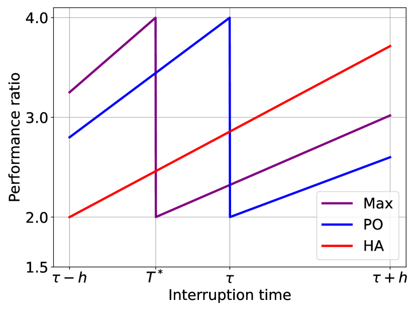
(a) Performance of Max.

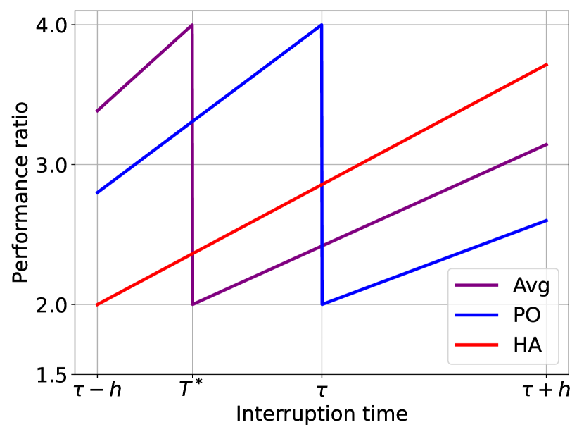
(b) Performance of Avg.

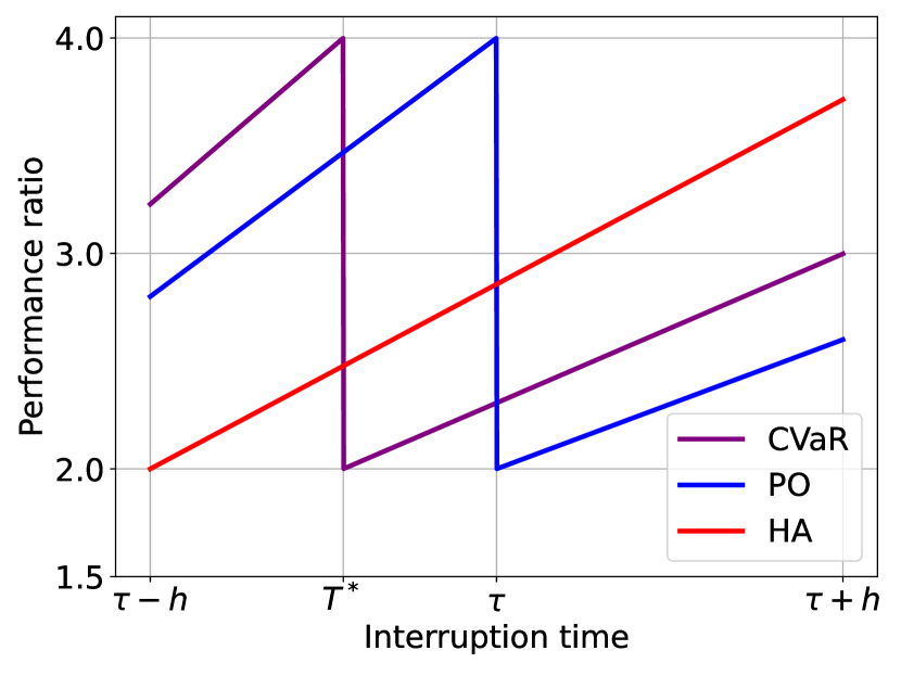
(c) Performance of ${\tt{CVaR}}$_0.5.

Figure 2: Performance ratios of our contract schedules, in comparison to HA and PO.

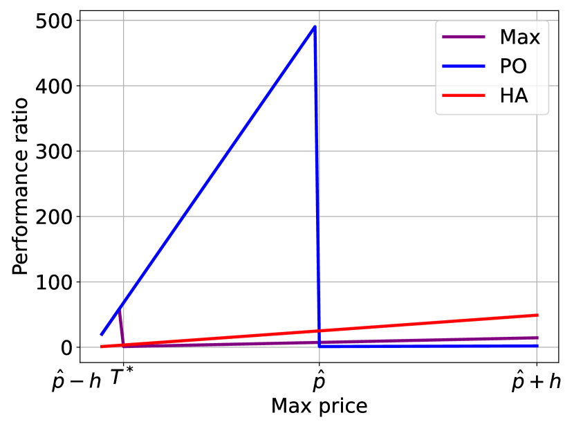
(a) Performance of Max.

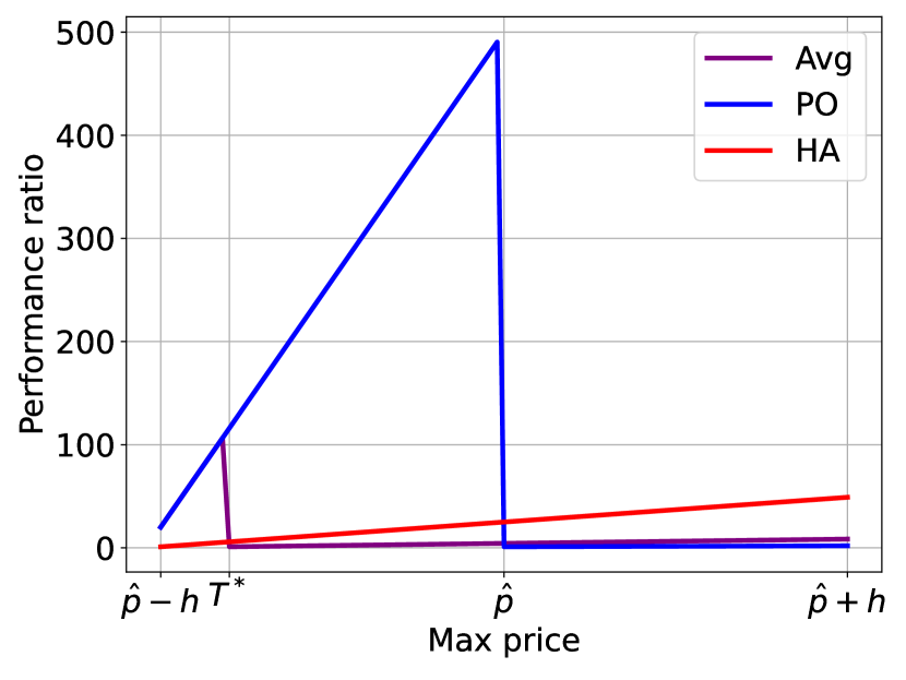
(b) Performance of Avg.

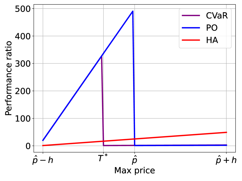
(c) Performance of ${\tt{CVaR}}$_0.5.

Figure 3: Performance ratios of our 1-max search algorithms, in comparison to HA and PO.

We evaluate our algorithms of Sections 3 and 4 which optimize the maximum and average distance as well as the CVaR. We refer to these algorithms as Max, Avg and CVaR_α.

5.1 Evaluation of contract schedules

We compare our schedules against two benchmarks, both of which are 4-robust [2].: i) The Pareto-Optimal schedule (PO) which optimizes the consistency, and must complete a contract at precisely the prediction $\tau$; and ii) The $h$-aware schedule (HA) that completes a contract at time $\tau-h$. Here, $h$ is an upper bound on the prediction error, i.e., the range of $\tau$ is in $[\tau-h,\tau+h]$. We thus allow a lot of power to this algorithm.

Figure 2 depicts the performance ratio of all algorithms as a function of the interruption time $T$, assuming a prediction $\tau=10^{6}$, and a range parameter $h=\tau/3$. For Max and Avg (Fig. 2(a) and 2(b)), we use a linear weight function in $[\tau-h,\tau+h]$, namely $w(T)=\max\{0,1-\frac{|T-\tau|}{h}\}$. For CVaR, (Fig 2(c)), the value of the risk parameter $\alpha$ is chosen to be $0.5$, and the distributional prediction is a symmetric Gaussian, normalized in $[\tau-h,\tau+h]$, with mean equal to $\tau$ and variance equal to 0.25. For Max, we compute its parameter $\lambda^{*}_{\max}$ using Algorithm 1, whereas for Avg and CVaR we rely on (7) and Theorem 5, respectively, and find $\lambda^{*}_{{\tt{avg}}}$ and $\lambda^{*}_{{\tt{CVaR}}}$ in $[1,2)$ using a distretization step equal to 0.001.

We observe that in all settings, our algorithms complete a contract at some time $T^{*}$ in $(\tau-h,\tau)$, unlike PO and HA that make extreme decisions, as can be observed by the discontinuity (drop) of the performance ratios at these times. This is in accordance with the motivation and the theoretical analysis of the schedules, that seeks a more nuanced choice of the parameter $\lambda$, which affects $T^{*}$. We also observe that in the entire interval $[T^{*},\tau+h]$, our algorithms strictly improve upon HA. They also significantly outperform PO in the interval $[T^{*},\tau]$, at the expense of a much smaller underperformance in $[\tau,\tau+h]$.

Table 1 summarizes the observed average improvement against PO and HA. Here, the row labeled “time vs X” refers to the percentage of time in $[\tau-h,\tau+h]$ for which an improvement is observed vs $X$, where $X=\{PO,HA\}$, whereas the row labeled “avg. ratio” refers to the average performance ratio of the schedule in this interval. We emphasize that the latter is a very pessimistic metric since it assigns equal importance to all values of error, whereas our algorithms prioritize small error values. To remove sensitivities on the choice of $\tau$, we repeated the experiments 100 times, choosing each time $\tau$ u.a.r in $[0.8\cdot 10^{6},1.2\cdot 10^{6}]$, and the table reports the average of the observed values.

5.2 Evaluation of 1-max search algorithms

We compare our algorithms against two benchmarks: The Pareto-Optimal algorithm (PO) of [36], and the $h$-aware algorithm (HA) of [3]. We choose $M=1000$ as the known upper bound on prices, thus $r$ must be such that $r\geq\sqrt{M}\approx 31.68$, where the latter is the competitive ratio. Since the HA algorithm does not guarantee any robustness, we will assume that $r$ is unbounded, which allows us to compare all algorithms under the same setting.

Figure 3 depicts the performance ratio of our algorithms, for $\hat{p}=500$, and $h=480$. Here, the horizontal axis represents maximum prices in worst-case inputs. Specifically, a point $x$ on the horizontal axis corresponds to a sequence that consists of infinitesimally increasing prices from 1 up to $x$, followed by a last price that is equal to 1. Such sequences maximize the performance ratios in both deterministic [36] and stochastic (Lemma 15) settings. Observe that, by definition, a point $x$ in the horizontal axis describes a sequence whose prediction error is $|\hat{p}-x|$, hence the plots depict the various performance ratios as a function of the prediction error. We use the same weight function and prediction distribution as in the setting of Section 5.1.

We observe that our algorithms choose a threshold $T^{*}$ in $(\hat{p}-h,\hat{p})$, i.e., in the interval between the thresholds of HA and PO, respectively. This is again in accordance with the motivation of the measures and their theoretical analysis. The plots show that our algorithms clearly outperform PO, and the performance gains are very significant when $p^{*}<\hat{p}$. Moreover, our algorithms outperform HA for a large fraction of the input sequences, namely for all sequences with maximum price larger than $T^{*}$. We quantify these improvements in Table 2, using the same setting as that of Table 1. Specifically, we repeat experiments 100 times, choosing in each of them a $\hat{p}$ u.a.r. in $[400,600]$, and $h=0.9\cdot\hat{p}$.

We conclude that for both problems, algorithms based on distance/risk measures capture the anticipated tradeoffs relative to PO and HA. More importantly, they demonstrate performance improvements for non-extreme values of the prediction error. We refer to Sections A.1 and A.2 for additional experimental results.

Table 1: Performance of schedules against PO and HA.

	Max	Avg	${\tt{CVaR}}$ 0.5	PO	HA
Avg Ratio	2.68	2.63	2.69	2.89	2.50
Time vs PO	23.1	33.1	24.9	–	–
Time vs HA	73.1	83.2	75.0	–	–

Table 2: Performance of 1-max algorithms against PO and HA.

	Max	Avg	${\tt{CVaR}}$ 0.5	PO	HA
Avg Ratio	9.26	10.51	58.03	127.08	24.9
Time vs PO	45.69	42.13	17.97	–	–
Time vs HA	96.04	92.48	68.32	–	–

6 Conclusion

We introduced new metrics rooted in decision theory that allow us to optimize the performance of a learning-augmented algorithm across an entire range of prediction error. We obtained theoretically optimal algorithms for two classic applications, which also outperform the known, extreme case approaches in practice. Our techniques can be applicable to other learning-augmented applications such as knapsack [18], secretary problems [8] and many variants of rent-or-buy problems such as ski rental [14, 32], for which single-valued ML-predictions have proved very useful. Another direction for future work is problems with multi-valued predictions such as packing problems [23]. Our framework can still apply in these more complex settings, since the error is defined by a distance norm between the predicted and the actual vector.

Appendix A Details from Section 5

A.1 Evaluation of contract schedules

In this section, we provide additional experimental results for evaluating our proposed schedules against the $h$-aware schedule (HA) and the Pareto-Optimal schedule (PO). The evaluation is conducted for various values of the parameter $h$, gaussian weight functions $w$, and different values of the parameter $\alpha$.

Our Gaussian weight function is defined along the lines of the normal distribution. Specifically,

$$w_{\text{gauss}}(T)=\begin{cases}\frac{1}{\sigma\sqrt{2\pi}}\exp\left(-\frac{1}{2}\left(\frac{T-\tau}{\sigma}\right)^{2}\right),&\text{if }T\in R_{\tau},\\ 0,&\text{otherwise},\end{cases}$$

where $\sigma=h/4$.

The results are presented for various values of $h$ and $\alpha$, and are summarized in the following figures:

• Figure 4: Performance ratios of Max, with weight function $w_{\text{gauss}}$ for different values of $h$, compared to HA and PO.

• Figure 5: Performance ratios of Avg with weight function $w_{\text{gauss}}$ for different values of $h$, compared to HA and PO.

• Figure 6: Performance ratios of CVaR for $h=0.2\cdot\tau$ and various values of $\alpha$, compared to HA and PO.

Tables 3, 4, 5 summarize our findings, using the same methodology as described in the main paper. We observe similar performance, across all variations, to those reported in Section 5.1.

We explain the behavior of the algorithms, as summarized in each of the three tables. In Table 3, we observe that the average performance ratios of our algorithms have increased, relative to the case of linear weights, which is attributed to the fact that the Gaussian weights prioritize small prediction errors to a higher extent than the linear function of the main paper. Intuitively, our schedules becomes “closer” to PO, since $T^{*}$ increases due to the gaussian weight, which explains why the performance ratios are higher, and closer to that of PO. Because $T^{*}$ increases relative to the linear weights, the percentage of time for which our schedules outperform HA decreases, as expected.

In Table 4, the value of $h$ is increased relative to that of Table 3. We expect to be further away from the behavior of PA and closer to that of HA, which is indeed observed in the figures of the performance plots. Similar conclusions hold for Table 5, where $h$ is even larger. We observe an overall monotone change in performance across the three tables, across all measured quantities.

Figure 6 depicts the performance of the ${\tt{CVaR}}$ schedules as a function of the parameter $\alpha$. First, note that as $\alpha\to 1$, we observe that the schedule 6(c) approaches HA, which is consistent with the theoretical interpretation we gave in Section 3.2. As $\alpha$ increases, we observe that $T^{*}$ comes to $\tau$, because the schedule becomes more risk-seeking, and risks an interruption during the execution of large contracts.

Table 3: Performance of our schedules against PO and HA with weight function $w_{\text{gauss}}$ and $h=\tau/5$.

	Max	Avg	${\tt{CVaR}}$ 0.5	PO	HA
Avg Ratio	2.74	2.72	2.69	2.89	2.50
Time vs PO	18.4	21.8	24.9	–	–
Time vs HA	68.5	71.9	75.0	–	–

Table 4: Performance of our schedules against PO and HA with weight function $w_{\text{gauss}}$ and $h=\tau/3$.

	Max	Avg	${\tt{CVaR}}$ 0.5	PO	HA
Avg Ratio	2.81	2.80	2.81	2.84	2.85
Time vs PO	17.0	19.8	22.1	–	–
Time vs HA	67.0	69.8	72.10	–	–

Table 5: Performance of our schedules against PO and HA with weight function $w_{\text{gauss}}$ and $h=0.4\cdot\tau$.

	Max	Avg	${\tt{CVaR}}$ 0.5	PO	HA
Avg Ratio	2.86	2.88	2.89	2.80	2.79
Time vs PO	15.9	18.0	19.9	–	–
Time vs HA	41.0	43.1	45.0	–	–

Table 6: Performance of our 1-max algorithms against PO and HA with weight function $w_{\text{gauss}}$ and $h=0.5\cdot\hat{p}$.

	Max	Avg	${\tt{CVaR}}$ 0.5	PO	HA
Avg Ratio	22.83	22.84	85.28	185.03	2.0
Time vs PO	41.58	41.58	22.77	–	–
Time vs HA	92.08	92.2	73.27	–	–

Table 7: Performance of our 1-max algorithms against PO and HA with weight function $w_{\text{gauss}}$ and $h=0.8\cdot\hat{p}$.

	Max	Avg	${\tt{CVaR}}$ 0.5	PO	HA
Avg Ratio	19.57	23.32	68.76	147.24	5.0
Time vs PO	37.62	35.64	18.81	–	–
Time vs HA	88.12	86.14	69.81	–	–

Table 8: Performance of our 1-max algorithms against PO and HA with weight function $w_{\text{gauss}}$ and $h=0.95\cdot\hat{p}$.

	Max	Avg	${\tt{CVaR}}$ 0.5	PO	HA
Avg Ratio	14.58	18.93	58.03	127.08	24.9
Time vs PO	35.64	32.67	16.83	–	–
Time vs HA	86.14	83.17	67.33	–	–

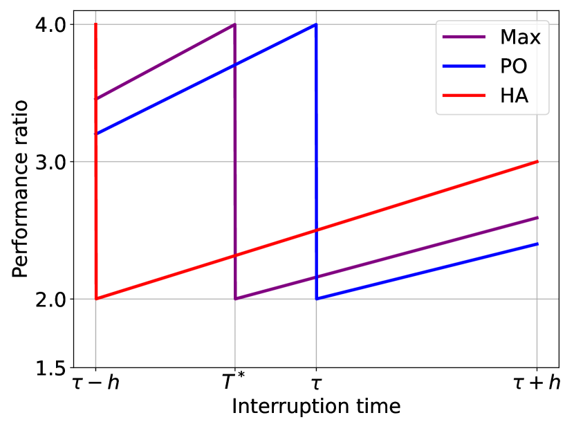
(a) Performance of Max for $h=\tau/5$.

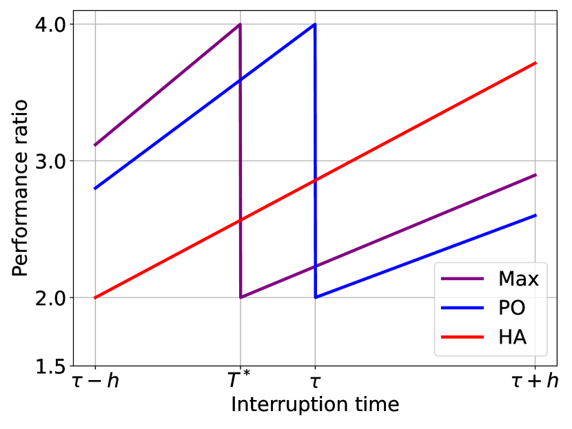
(b) Performance of Max for $h=\tau/3$.

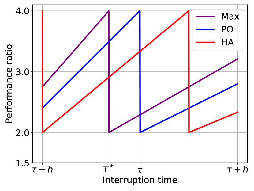
(c) Performance of Max for $h=0.4\cdot\tau$.

Figure 4: Performance ratios of Max with weight function $w_{\text{gauss}}$ for different values of $h$, in comparison to HA and PO.

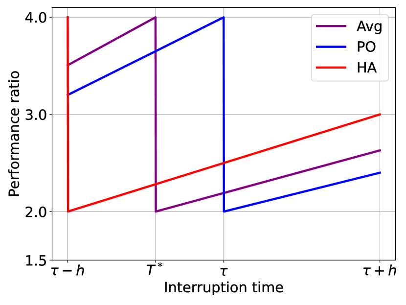
(a) Performance of Avg for $h=\tau/5$.

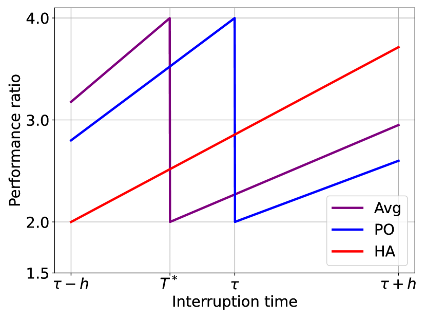
(b) Performance of Avg for $h=\tau/3$.

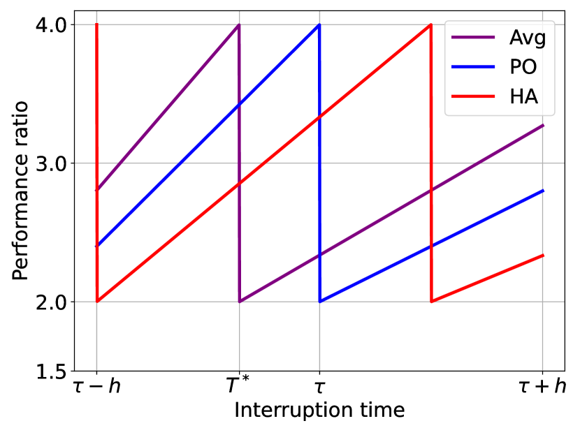
(c) Performance of Avg for $h=0.4\cdot\tau$.

Figure 5: Performance ratios of Avg with weight function $w_{\text{gauss}}$ for different values of $h$, in comparison to HA and PO.

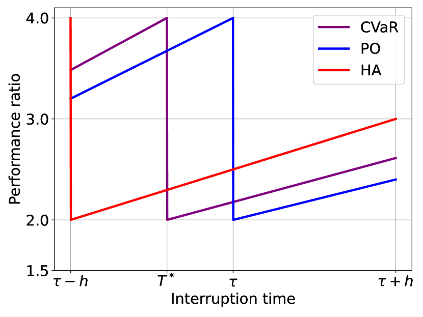
(a) Performance of ${\tt{CVaR}}$_0.0.

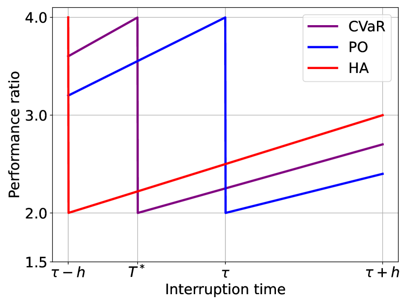
(b) Performance of ${\tt{CVaR}}$_0.7.

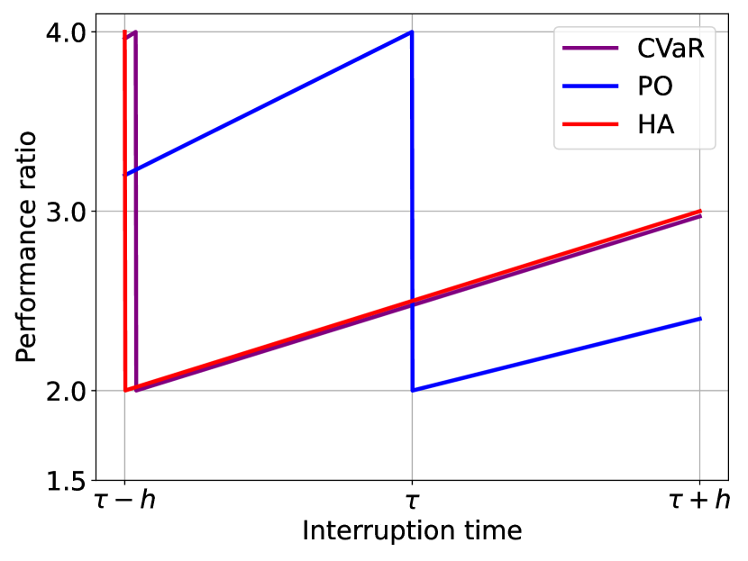
(c) Performance of ${\tt{CVaR}}$_0.999.

Figure 6: Performance ratios of CVaR for $h=\tau/5$ and different values of $\alpha$.

A.2 Evaluation of 1-max Search Algorithms

We give additional experimental results for our 1-max search algorithms. Similar to contract scheduling, we consider varying values of $h$, a gaussian weight function $w$, and different values of the parameter $\alpha$. The gaussian weight function is as defined in the previous section, with $T$ being replaced by $p^{*}$. We summarize the results in a series of figures that compare the performance ratios of our 1-max search algorithms against benchmark algorithms HA and PO.

• Figure 7: Performance ratios of Max with weight function $w_{\text{gauss}}$ for different values of $h$, in comparison to HA and PO.

• Figure 8: Performance ratios of Avg with weight function $w_{\text{gauss}}$ for different values of $h$, in comparison to HA and PO.

• Figure 9: Performance ratios of CVaR with $h=0.95\cdot\hat{p}$ and different values of $\alpha$.

Tables 6, 7, 8 summarize our findings. We observe that the average performance ratio of PO decreases with $h$, whereas the opposite holds for HA, as expected from their statements. Our algorithms show an overall decreasing average performance ratio as a function of $h$, which can be explained by the fact that the threshold $T^{*}$ of our algorithms decreases with $h$, which in turn helps reduce the “jump” in the performance ratio which we observe for maximum prices close, but smaller than $T^{*}$.

For CVaR, our findings can be explained similarly to the contract scheduling setting, and are thus consistent with the theoretical interpretation of Section 4.2.

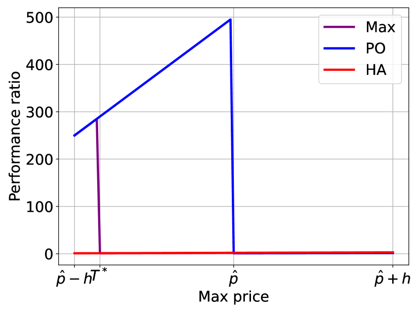
(a) Performance of Max for $h=0.5\cdot\hat{p}$.

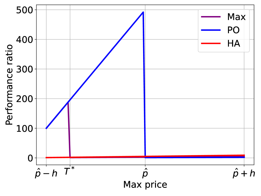
(b) Performance of Max for $h=0.8\cdot\hat{p}$.

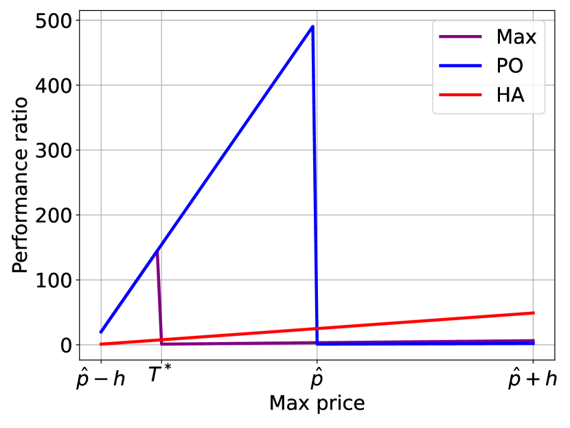
(c) Performance of Max for $h=0.95\cdot\hat{p}$.

Figure 7: Performance ratios of our 1-max search algorithm Max with weight function $w_{\text{gauss}}$ for different values of $h$, in comparison to HA and PO.

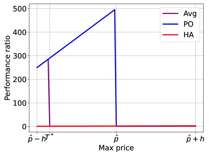
(a) Performance of Avg for $h=0.5\cdot\hat{p}$.

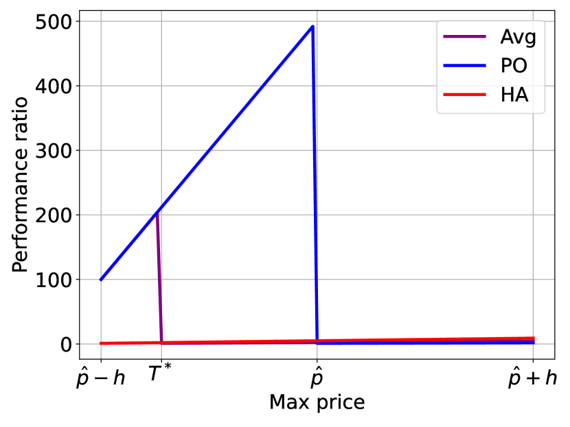
(b) Performance of Avg for $h=0.8\cdot\hat{p}$.

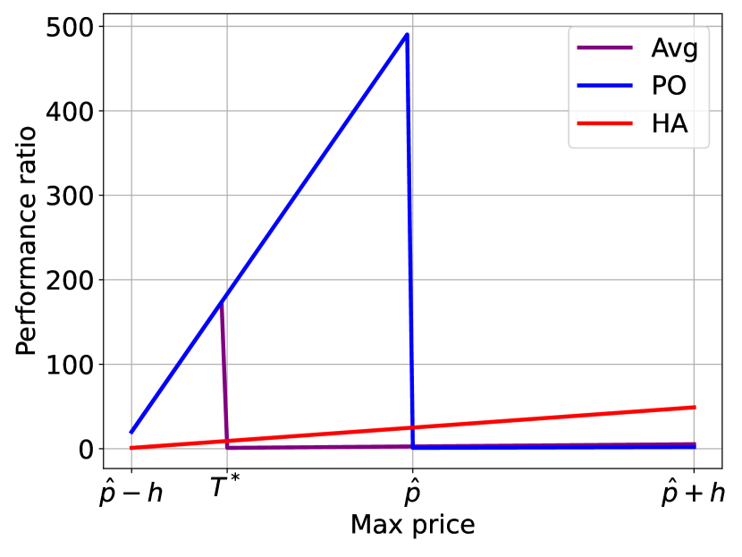
(c) Performance of Avg for $h=0.95\cdot\hat{p}$.

Figure 8: Performance ratios of our 1-max search algorithm Avg with weight function $w_{\text{gauss}}$ for different values of $h$, in comparison to HA and PO.

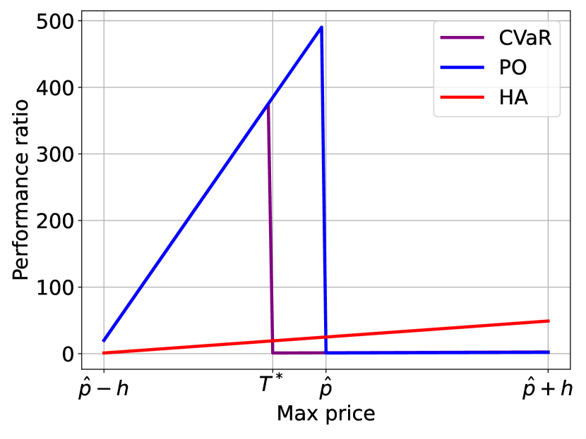
(a) Performance of ${\tt{CVaR}}$_0.0.

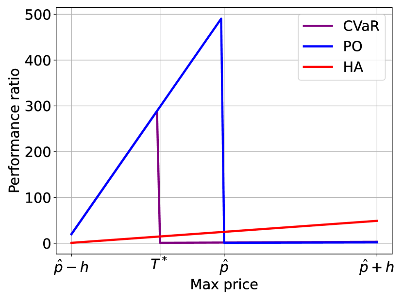
(b) Performance of ${\tt{CVaR}}$_0.7.

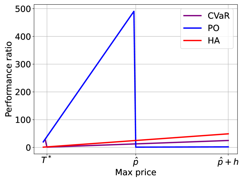
(c) Performance of ${\tt{CVaR}}$_0.999.

Figure 9: Performance ratios of our 1-max search algorithm CVaR with $h=0.95\cdot\hat{p}$ and different values of $\alpha$.

Real Data for the 1-Max Search Problem

In this section, we provide an example of computational evaluation of our algorithms using real-world data. As a benchmark, we used the exchange rates of EUR to four other currencies: CHF, USD, JPY, and GBP. Each exchange rate represents a sequence $\sigma$ of 6672 prices over a span of 25 years.

For generating predictions, we consider a random value $z$ sampled from a normal distribution with a mean equal to zero, standard deviation of $1/2$ and truncated to the interval $[-1,+1]$. This value is then scaled by the error upper bound $h$, generating the predicted value $\hat{p}=p^{*}+h\cdot z.$

The error upper bound $h$ is generated by dividing the input sequence $\sigma$ into 8 equal length intervals. For each interval $i$, the maximum exchange rate $M_{i}$ is considered. The value of $h$ is then defined as the span of these values:

$$h=\max_{i\in\{1,\dots,8\}}M_{i}-\min_{i\in\{1,\dots,8\}}M_{i}.$$

Recall that in 1-max search, if all prices are below the chosen threshold, the algorithm needs to sell at lowest price 1. However, in this experimental setup we use the lowest price in the sequence as this lowest final price.

To account for the randomness in the predictions, we performed 10000 runs and computed the average competitive ratio. A linear weight function was used in the evaluation of the algorithms Max and Avg.

The final results are presented in the Table 9. Since the input sequence in real-life scenarios is not a worst-case sequence and the range of prices varies depending on the currency, it is challenging to determine which algorithm performs best overall. As shown in the table, the competitive ratios vary significantly depending on the currency. For example, ${\tt{CVaR}}$_0.5 algorithm performs better for USD and JPY, while Max and Avg algorithms demonstrate better competitive performance for CHF. This variability highlights the dependence of algorithm performance on the specific characteristics of the input data.

Table 9: Competitive ratios for the PO, HA, Max, Avg, and ${\tt{CVaR}}$ _0.5 algorithms.

Currency	PO	HA	Max	Avg	${\tt{CVaR}}$ 0.5
CHF	1.5571	1.7824	1.4926	1.3744	1.6102
GBP	1.7134	1.1573	1.7134	1.7134	1.7134
JPY	1.9640	1.0876	1.0876	1.0876	1.0464
USD	1.9377	1.2124	1.0611	1.0335	1.0242

References

- [1] Spyros Angelopoulos and Shendan Jin “Earliest-Completion Scheduling of Contract Algorithms with End Guarantees” In Proceedings of the 28th International Joint Conference on Artificial Intelligence, (IJCAI), 2019, pp. 5493–5499
- [2] Spyros Angelopoulos and Shahin Kamali “Contract Scheduling with Predictions” In J. Artif. Intell. Res. 77, 2023, pp. 395–426
- [3] Spyros Angelopoulos, Shahin Kamali and Dehou Zhang “Online Search with Best-Price and Query-Based Predictions” In Proceedings of the 36th AAAI Conference on Artificial Intelligence AAAI Press, 2022, pp. 9652–9660
- [4] Spyros Angelopoulos and Alejandro López-Ortiz “Interruptible Algorithms for Multi-Problem Solving” In Proceedings of the 21st International Joint Conference on Artificial Intelligence (IJCAI), 2009, pp. 380–386
- [5] Spyros Angelopoulos, Alejandro López-Ortiz and Angele Hamel “Optimal Scheduling of Contract Algorithms with Soft Deadlines” In Proceedings of the 23rd AAAI Conference on Artificial Intelligence (AAAI), 2008, pp. 868–873
- [6] Spyros Angelopoulos, Marcin Bienkowski, Christoph Dürr and Bertrand Simon “Contract Scheduling with Distributional and Multiple Advice” In Proceedings of the Thirty-Third International Joint Conference on Artificial Intelligence, IJCAI, 2024, pp. 3652–3660
- [7] Spyros Angelopoulos, Marcin Bienkowski, Christoph Dürr and Bertrand Simon “Contract Scheduling with Distributional and Multiple Advice” arXiv:2404.12485 In Proceedings of the 33rd International Joint Conference on Artificial Intelligence (IJCAI), 2024
- [8] Antonios Antoniadis, Themis Gouleakis, Pieter Kleer and Pavel Kolev “Secretary and online matching problems with machine learned advice” In Discret. Optim. 48.Part 2, 2023, pp. 100778
- [9] Yossi Azar, Debmalya Panigrahi and Noam Touitou “Online Graph Algorithms with Predictions” In Proceedings of the 2022 ACM-SIAM Symposium on Discrete Algorithms, SODA SIAM, 2022, pp. 35–66
- [10] Etienne Bamas, Andreas Maggiori and Ola Svensson “The primal-dual method for learning augmented algorithms” In Advances in Neural Information Processing Systems 33, 2020, pp. 20083–20094
- [11] Daniel S. Bernstein, Lev Finkelstein and Shlomo Zilberstein “Contract Algorithms and Robots on Rays: Unifying Two Scheduling Problems” In Proceedings of the 18th International Joint Conference on Artificial Intelligence (IJCAI), 2003, pp. 1211–1217
- [12] Daniel S. Bernstein, T.. Perkins, Shlomo Zilberstein and Lev Finkelstein “Scheduling Contract Algorithms on Multiple Processors” In Proceedings of the 18th AAAI Conference on Artificial Intelligence (AAAI), 2002, pp. 702–706
- [13] Allan Borodin and Ran El-Yaniv “Online computation and competitive analysis” Cambridge University Press, 1998
- [14] Nicolas Christianson, Junxuan Shen and Adam Wierman “Optimal robustness-consistency tradeoffs for learning-augmented metrical task systems” In AISTATS 206, Proceedings of Machine Learning Research PMLR, 2023, pp. 9377–9399
- [15] Nicolas Christianson, Bo Sun, Steven H. Low and Adam Wierman “Risk-Sensitive Online Algorithms (Extended Abstract)” In The Thirty Seventh Annual Conference on Learning Theory (COLT) 247, Proceedings of Machine Learning Research PMLR, 2024, pp. 1140–1141
- [16] Jhoirene Clemente, Juraj Hromkovič, Dennis Komm and Christian Kudahl “Advice complexity of the online search problem” In International Workshop on Combinatorial Algorithms, 2016, pp. 203–212 Springer
- [17] Peter Damaschke, Phuong Hoai Ha and Philippas Tsigas “Online search with time-varying price bounds” In Algorithmica 55.4 Springer, 2009, pp. 619–642
- [18] Mohammadreza Daneshvaramoli et al. “Competitive Algorithms for Online Knapsack with Succinct Predictions” In arXiv preprint arXiv:2406.18752, 2024
- [19] Ilias Diakonikolas et al. “Learning online algorithms with distributional advice” In International Conference on Machine Learning, 2021, pp. 2687–2696 PMLR
- [20] Alex Elenter, Spyros Angelopoulos, Christoph Dürr and Yanni Lefki “Overcoming Brittleness in Pareto-Optimal Learning-Augmented Algorithms” In Proceedings of the 37th Annual Conference on Neural Information Processing Systems (NeurIPS), 2024
- [21] Tom Fawcett “An introduction to ROC analysis” In Pattern recognition letters 27.8 Elsevier, 2006, pp. 861–874
- [22] Sreenivas Gollapudi and Debmalya Panigrahi “Online Algorithms for Rent-Or-Buy with Expert Advice” In Proceedings of the 36th International Conference on Machine Learning, ICML 97, Proceedings of Machine Learning Research PMLR, 2019, pp. 2319–2327
- [23] Sungjin Im, Ravi Kumar, Mahshid Montazer Qaem and Manish Purohit “Online knapsack with frequency predictions” In Advances in Neural Information Processing Systems 34, 2021, pp. 2733–2743
- [24] Silvio Lattanzi, Thomas Lavastida, Benjamin Moseley and Sergei Vassilvitskii “Online Scheduling via Learned Weights” In Proceedings of the 2020 ACM-SIAM Symposium on Discrete Algorithms SIAM, 2020, pp. 1859–1877
- [25] Thomas Lavastida, Benjamin Moseley, R. Ravi and Chenyang Xu “Learnable and Instance-Robust Predictions for Online Matching, Flows and Load Balancing” In 29th Annual European Symposium on Algorithms, ESA) 204, LIPIcs, 2021, pp. 59:1–59:17
- [26] Russell Lee, Bo Sun, Mohammad Hajiesmaili and John C.. Lui “Online Search with Predictions: Pareto-optimal Algorithm and its Applications in Energy Markets” In e-Energy ACM, 2024, pp. 50–71
- [27] Jialiang Li and Jason P Fine “Weighted area under the receiver operating characteristic curve and its application to gene selection” In Journal of the Royal Statistical Society Series C: Applied Statistics 59.4 Oxford University Press, 2010, pp. 673–692
- [28] Alexander Lindermayr and Nicole Megow “Repository of works on algorithms with predictions” Accessed: 2025-01-01, https://algorithms-with-predictions.github.io, 2025
- [29] Alejandro López–Ortiz, Spyros Angelopoulos and Angele Hamel “Optimal Scheduling of Contract Algorithms for Anytime Problem-Solving” In J. Artif. Intell. Res. 51, 2014, pp. 533–554
- [30] Thodoris Lykouris and Sergei Vassilvtiskii “Competitive Caching with Machine Learned Advice” In International Conference on Machine Learning, 2018, pp. 3296–3305 PMLR
- [31] Esther Mohr, Iftikhar Ahmad and Günter Schmidt “Online algorithms for conversion problems: a survey” In Surveys in Operations Research and Management Science 19.2 Elsevier, 2014, pp. 87–104
- [32] Manish Purohit, Zoya Svitkina and Ravi Kumar “Improving Online Algorithms via ML Predictions” In Advances in Neural Information Processing Systems 31, 2018, pp. 9661–9670
- [33] R Tyrrell Rockafellar and Stanislav Uryasev “Optimization of conditional value-at-risk” In Journal of risk 2, 2000, pp. 21–42
- [34] Stuart J. Russell and Shlomo Zilberstein “Composing real-time Systems” In Proceedings of the 12th International Joint Conference on Artificial Intelligence (IJCAI), 1991, pp. 212–217
- [35] Sergey Sarykalin, Gaia Serraino and Stan Uryasev “Value-at-risk vs. conditional value-at-risk in risk management and optimization” In State-of-the-art decision-making tools in the information-intensive age Informs, 2008, pp. 270–294
- [36] Bo Sun et al. “Pareto-optimal learning-augmented algorithms for online conversion problems” In Advances in Neural Information Processing Systems 34, 2021, pp. 10339–10350
- [37] Alexander Wei and Fred Zhang “Optimal Robustness-Consistency Trade-offs for Learning-Augmented Online Algorithms” In Proceedings of the 33rd Conference on Neural Information Processing Systems (NeurIPS), 2020
- [38] Ran El-Yaniv “Competitive solutions for online financial problems” In ACM Computing Surveys 30.1, 1998, pp. 28–69
- [39] Ran El-Yaniv, Amos Fiat, Richard M Karp and Gordon Turpin “Optimal search and one-way trading online algorithms” In Algorithmica 30.1 Springer, 2001, pp. 101–139
- [40] Shlomo Zilberstein, Francois Charpillet and Philippe Chassaing “Optimal Sequencing of Contract Algorithms.” In Ann. Math. Artif. Intell. 39.1-2, 2003, pp. 1–18