Non-halo structures and their effects on gravitationally lensed galaxies

While the $\Lambda$CDM model succeeds on large scales, its validity on smaller scales remains uncertain. Recent works suggest that non-halo dark matter structures, such as filaments and walls, could significantly influence gravitational lensing and that the importance of these effects depends on the dark matter model: in warm dark matter scenarios, fewer low-mass objects form and thus their mass is redistributed into the cosmic-web. We investigate these effects on galaxy-galaxy lensing using fragmentation-free Warm Dark Matter (WDM) simulations with particle masses of m_χ = 1 keV and m_χ = 3 keV. Although these cosmological scenarios are already observationally excluded, the fraction of mass falling outside of haloes grows with the thermal velocity of the dark matter particles, which allows for the search for first-order effects. We create mock datasets, based on gravitationally-lensed systems from the BELLS-Gallery, incorporating non-halo contributions from these simulations to study their impact in comparison to mocks where the lens has a smooth mass distribution. Using Bayesian modelling, we find that perturbations from WDM non-halo structures produce an effect on the inferred parameters of the main lens and shift the reconstructed source position. However, these variations are subtle and are effectively absorbed by standard elliptical power-law lens models, making them challenging to distinguish from intrinsic lensing features. Most importantly, non-halo perturbation does not appear as a strong external shear term, which is commonly used in gravitational lensing analyses to represent large-scale perturbations. Our results demonstrate that while non-halo structures can affect the lensing analysis, the overall impact remains indistinguishable from variations of the main lens in colder WDM and CDM scenarios, where non-halo contributions are smaller.

1 Introduction

One of the long-lasting problems and main goals of modern cosmology is to understand the nature of dark matter (see e.g. Bosma, 1981; Bullock & Boylan-Kolchin, 2017; Zavala & Frenk, 2019). In the Lambda Cold Dark Matter ($\Lambda$CDM) paradigm, often referred to as the standard model of cosmology, dark matter particles are assumed to be non-relativistic, cold, and make up for $85$ per cent of the matter content and approximately $27$ per cent of the total mass-energy budget of the Universe (see Planck Collaboration (2020)). $\Lambda$CDM is widely used in numerical simulations as it can accurately reproduce and predict the large-scale structure of the Universe (Frenk & White, 2012; V. Springel & White, 2006), and provides a physical explanation for several crucial phenomena such as the CMB (Cosmic Microwave Background) (Planck Collaboration, 2011), the large scale distribution of galaxies, and the accelerated expansion of the Universe.

Several models have been proposed as alternatives to CDM (see e.g. Bullock & Boylan-Kolchin, 2017; Bertone & Tait, 2018, for reviews) to reconcile predictions from $\Lambda$CDM with observations on galactic and sub-galactic scales. Here, we will focus on models that suppress small-scale structure formation, specifically thermal relic Warm Dark Matter (WDM) models (Bode et al., 2001). In these models, dark matter particles are produced in an equilibrium state with a non-negligible initial thermal velocity. This initial thermal velocity dispersion allows the dark matter particles to free-stream out of the gravitational potential wells of smaller perturbations and, as a result, suppresses the gravitational collapse of these perturbations.

Strong gravitational lensing allows one to measure the dark matter distribution on the sub-galactic scale where the difference between models is large. Hence, it provides a robust avenue to test predictions from different dark matter models (Dalal & Kochanek, 2002; Xu et al., 2009; Vegetti et al., 2018; Gilman et al., 2020; Powell et al., 2023) through the detection of low-mass dark-matter haloes, of which the abundance is highly sensitive to the nature of dark matter. It also proves to be complementary to stellar streams in the Milky Way (Banik et al., 2021), Lyman-$\alpha$ (Iršič et al., 2024) and Milky Way satellites analysis regarding the search for thermal relic dark matter (Nadler et al., 2021; Enzi et al., 2021). However, one needs a careful understanding of all possible sources of systematic errors. For example, Richardson et al. (2022), hereafter cited as R22, have shown that material outside of haloes, such as filaments and walls, can have a non-negligible effect on the relative fluxes of quadruply-lensed quasars, comparable to that of low-mass haloes. Hence, leading to a potential bias in favour of colder dark matter models when neglected.

In this paper, we investigate whether these non-halo structures also affect the surface brightness distribution of strongly lensed arcs. The latter is sensitive to local changes of the first derivative of the lensing potential in a way that is strongly dependent on the angular resolution of the data: the better the resolution, the smaller the angular size of the perturbations that can be detected (Despali et al., 2019). Here, we focus on mock images created to reproduce observations by the Hubble Space Telescope (HST), which have been studied by Shu et al. (2016b), Nightingale et al. (2023) and Ritondale et al. (2018) as part of the BELLS-Gallery sample. In particular, we aim to study the effect of non-halo structures in different WDM scenarios. We use the new, fragmentation-free simulations from R22 to add non-halo structures to mock lensing datasets and test if they can be detected and distinguished from the effect of the main lens. Recent studies on quadruply lensed quasars have ruled out DM models with $m_{\chi}<5.2$ keV, favouring colder DM particles (Hsueh et al., 2019; Gilman et al., 2019). However, these analyses neglect the effect of material outside of haloes. Analysis of the WDM non-halo structures could lead to a less strict constraint. Therefore, following the parameters used in R22 and their numerical requirements, we consider two models with WDM particle masses $m_{\chi}=1$ and $m_{\chi}=3$ keV. Although $m_{\chi}=1$ keV is already ruled out by observations, we use it as a limiting case.

The paper is structured as follows: in Sect. 2 we present the data from our WDM simulation and for the gravitational imaging. In Sect. 3 we detail the mock data which we model in Sect. 4. Then in Sect. 5 we present and comment our results, and present our conclusions in Sect. 6.

2 Simulations

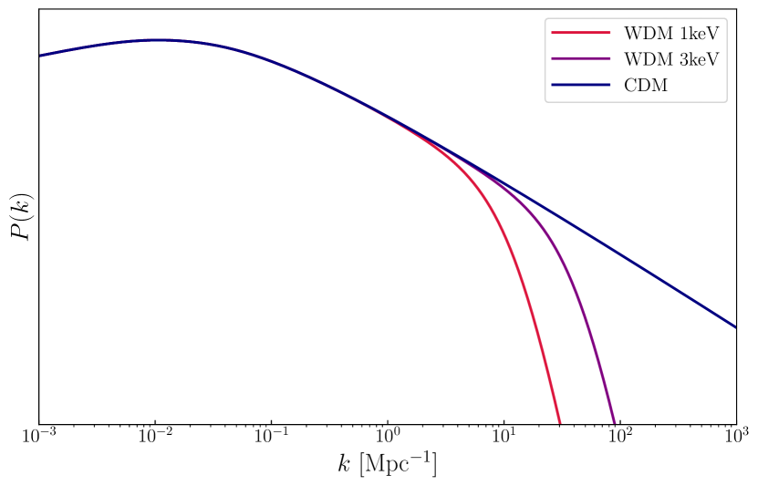
Figure 1: Power spectra for CDM, $m_{\chi}=1$ keV and $m_{\chi}=3$ keV WDM. The WDM power spectra correspond to low-pass filtered versions of the CDM power spectrum. The vertical axis is unitless and arbitrarily normalised. The free-streaming scale is a function of the dark matter particle mass $m_{\chi}$, and is directly related to the cut-off scale.

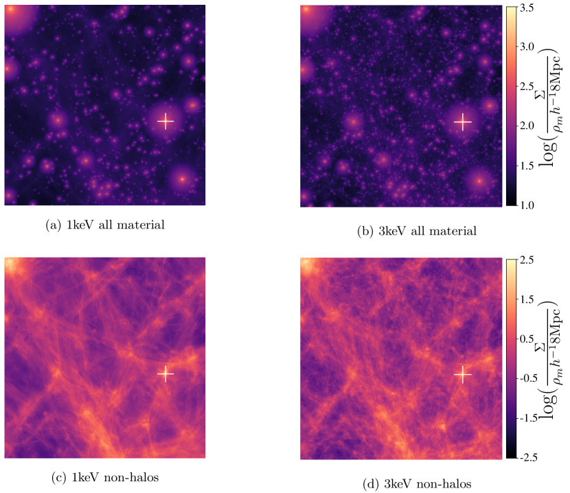
Figure 2: Upper panel: Full projected data from both simulations from R22. Each square has a side length of $8h^{-1}$Mpc, and corresponds to a $80h^{-1}$Mpc projection. Panel (b) contains much fewer small-scale dark matter haloes than panel (a) as the free-streaming length is longer in 1 keV than in 3 keV WDM. Lower panel: Non-Halo projected data from both simulations from R22. Each square has a side length of $8h^{-1}$Mpc¹, and corresponds to a $80h^{-1}$Mpc¹ projection. Panel (d) contains smoother and less clumpy structures at small scales than panel (c). The markers are all at the same coordinates and show the regions from which we select the non-halo material used as additional perturbations in our gravitationally lensed systems. They correspond to the highest density of non-halo material in both simulations and to the densest halo in both simulations if we exclude the cut ones in the top-left corner.

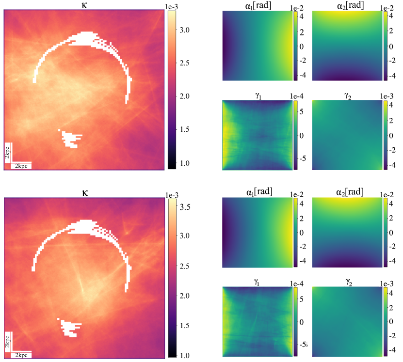
Figure 3: $20\times 20$ kpc² maps of the convergence, deflection angle components, and shear components for the non-halo material in two regions around haloes at the same coordinates in the 3 keV (top) and 1 keV (bottom) simulations from R22. The deflection angle maps are used to add the effect of non-halo structures on top of the deflection from the elliptical power law lenses in our datasets. The positions of the non-halo material from which we compute these convergence maps are marked in Fig. 2. They are the same in both simulations. The white contours are based on the arc light image of SDSSJ110+3649 projected at $z=0.733$.

2.1 Simulation parameters and models

In this work, we analyse two runs from the suite of WDM simulations presented in Stücker et al. (2022). Each volume represents a $(20h^{-1}{\rm Mpc})^{3}$ periodic box, run with cosmological WDM initial conditions generated using MUSIC (Hahn & Abel, 2013). Both simulations were run using the same initial Gaussian random noise field and with the same cosmological parameters, $h=0.679$, $\Omega_{\rm m}=0.3051$, $\Omega_{\Lambda}=0.6949$, $\Omega_{\rm K}=0$, and $\sigma_{8}=0.8154$ (Planck Collaboration, 2020), but differ with regards to the dark matter model they represent. In particular, we use two volumes replicating cosmological structure formation in the presence of thermal relic dark matter with a particle mass of either, $m_{\chi}=1{\rm keV}$ or $m_{\chi}=3{\rm keV}$, which we will hereafter refer to as the 1 keV or 3 keV simulations respectively.

In WDM cosmologies the thermal velocity of DM particles leads them to have a finite free-streaming length (Bode et al., 2001),

$$\lambda_{\rm s}=\frac{0.048}{h\text{Mpc}^{-1}}\left(\frac{\Omega_{\chi}}{0.4}\right)^{0.15}\left(\frac{h}{0.65}\right)^{1.3}\left(\frac{1\text{keV}}{m_{\chi}}\right)^{1.15}\left(\frac{1.5}{g_{\chi}}\right)^{0.29},$$ (1)

which depends on the particle mass $m_{\chi}$, the dark matter density in units of the critical density of the Universe, $\Omega_{\chi}$, and $g_{\chi}$, a dimensionless factor which accounts for the number of degrees of freedom of the dark matter particles, here we adopt $g_{\chi}=1.5$, the value corresponding to the case of sterile neutrinos.

This free-streaming motion is considered negligible in CDM, but in the case of WDM leads to a small scale dampening to the power spectrum which is modelled here using the Bode et al. (2001) transfer function,

$$P_{\rm WDM}(\textbf{k})=(1+(\lambda_{s}k)^{2})^{-10}P_{\rm CDM}(\textbf{k}),$$ (2)

where $P(\textbf{k})$ is the scale-dependant power spectrum, and k is the wavenumber vector. The resulting dampening to the power spectrum is shown in Fig. 1.

Beyond smoothing out density fluctuations, the free-streaming of the WDM particles allows them to escape small scale gravitational potential fluctuations,which effectively suppresses structure formation below the half-mode mass scale,

$$M_{\rm hm}=\frac{4\pi}{3}\rho_{\rm m}\left(\frac{\lambda_{\rm hm}}{2}\right)^{3}.$$ (3)

where $\rho_{\rm m}$ is the mean matter density of the Universe, and

$$\lambda_{\rm hm}=2\pi\lambda_{\rm s}(2^{1/5}-1)^{-1/2}.$$ (4)

$M_{\rm hm}$ corresponds to the mass at which the WDM halo abundance is suppressed by a factor of two with respect to its CDM counterpart (Viel et al., 2005; Schneider et al., 2012). The WDM models used here respectively result in a half-mode mass of $M_{hm}=2.5\times 10^{10}h^{-1}$M_⊙ for the 1 keV model and $M_{hm}=5.7\times 10^{8}h^{-1}$M_⊙ for the 3 keV model. WDM models are commonly associated only with the lack of low-mass structures, which is their main signature. However, it is worth noting that the material which is not confined to haloes remains within non-halo structures, for instance, R22 find that, at $z=0$, the fraction of matter outside of haloes represents $f_{\rm non-halo}=45.7$ per cent of the total dark matter mass in the 1 keV model, and respectively $f_{\rm non-halo}=34.8$ per cent in the 3 keV model. This means that in WDM models, more matter is redistributed in the smooth cosmic-web large-scale structures with respect to CDM.

2.2 Avoiding artificial fragmentation

While large-scale structure formation in CDM models has been very successfully reproduced using $N$-body simulations, this has not been the case for WDM models. Indeed, it has been found that in $N$-body WDM simulations the smoother density field will artificially fragment due to discreteness effects (Wang & White, 2007) resulting in a large population of spurious small mass haloes. Although, methods have been developed to identify and remove this spurious population (see e.g. Lovell et al., 2014; Stücker et al., 2022), these artificial haloes have nonetheless prohibited the study of the smoother regions of the density fields in this type of simulation.

To circumvent this issue another approach has been developed (Abel et al., 2012; Shandarin et al., 2012; Hahn & Abel, 2013) which relies on the assumption that the DM distribution function only occupies a three dimensional hyper surface of the full six dimensional phase space. In these simulations, the phase space distribution function is tessellated using a set of tracer particles, which can in turn be used to calculate the temporal evolution of the full phase space distribution function with much higher accuracy. These methods however break down inside virialised structures due to chaotic mixing, requiring an exponentially large number of tracer particles to accurately trace these systems (Hahn & Angulo, 2016; Sousbie & Colombi, 2016).

The simulations used here, make use of a hybrid tessellation-$N$-body method (Stücker et al., 2020, 2022), which dynamically separates particles into four categories namely, voids, walls, filaments, and haloes. For the three first categories, the phase space distribution function is tessellated using $N_{\rm V}=256^{3}$ particles, while the final category is modelled using $N_{\rm T}=512^{3}$ tracer particles of mass $m_{\rm T}=5.0\cdot 10^{6}h^{-1}{\rm M}_{\odot}$ which are released in regions where the density field has collapsed along three dimensions, i.e. inside haloes. This hybrid approach maintains the efficiency of $N$-body inside haloes while allowing the large-scale distribution function to be traced to very high accuracy.

An additional advantage of the hybrid tessellation-$N$-body approach is that it allows, in post-processing, to effectively interpolate the smooth density field down to arbitrarily small masses. allowing the creation of extremely high-resolution density maps outside of haloes. It is using this property that R22 were able to project ten $(8\times 8\times 8)h^{-3}{\rm Mpc}^{3}$ sub volumes with an effective mass resolution of $\sim 20h^{-1}{\rm M}_{\odot}$, which, once put together, represent a continuous $(80\times 8\times 8)h^{-3}{\rm Mpc}^{3}$ projection. These projected density maps are shown in Fig. 2, where in the upper panels we show all the matter inside the simulation, except the halos that have been fitted and replaced by spherical NFW profiles to reduce the numerical noise. In the lower panels we only show the matter present in non-halo structures, showing the 1 keV and 3 keV simulations in the left and right panels respectively. As discussed previously, we can clearly see that the 3 keV simulation contains many more low-mass haloes and that the 1 keV simulation appears far smoother with fewer visible clumps in the filaments and walls.

Using these projections, R22 investigate the impact of non-halo structures on flux-ratio anomalies in multiply imaged quasars. By sampling 1000 random lines of sight, the authors show that in a $m_{\chi}=3$ keV scenario, neglecting the non-halo material can lead to an underestimation of the flux ratio anomalies by five to ten per cent, which increases substantially for the warmer 1 keV model. From this analysis, the authors conclude that non-halo material should be included in rigorous models and that their inclusion can affect the constraints on the DM particle mass.

Table 1: Parameters for the WDM cosmological simulations used in R22 and in this work. The cosmological parameters are the best-fit values from the Planck collaboration 2018 results from the Planck collaboration 2018 results (Planck Collaboration, 2020).

Parameter	1 keV	3 keV
$h$	0.679	-
$\Omega_{\rm m}$	0.3051	-
$\Omega_{\Lambda}$	0.6949	-
$\Omega_{\rm K}$	0	-
$\sigma_{8}$	0.8154	-
$N_{\rm V}$	2563	-
$N_{\rm T}$	5123	-
$m_{\rm T}$ $[h^{-1}$M${}_{\odot}]$	$5.0\cdot 10^{6}$	-
$f_{\rm non-halo}$	45.7%	34.8%
$M_{\rm hm}$ $[h^{-1}$M${}_{\odot}]$	$2.5\cdot 10^{10}$	$5.7\cdot 10^{8}$
$\lambda_{\rm s}$ [kpc]	5.06	1.44
$\lambda_{\rm hm}$ [kpc]	82.6	23.4

2.3 Lensing maps

From the simulated non-halo surface density maps (lower panels in Fig. 2), we create the convergence $\kappa$ defined as the ratio between the surface mass density and a critical surface density which is a function of the lens and the source angular diameters:

$$\kappa\equiv\frac{\Sigma(\boldsymbol{x})}{\Sigma_{\rm cr}},\text{ with }\Sigma_{\rm cr}=\frac{c^{2}}{4\pi G}\frac{D_{\rm S}}{D_{\rm L}D_{\rm LS}},$$ (5)

with $c$ the speed of light, $G$ the gravitational constant, and $D_{\rm L}$, $D_{\rm S}$, and $D_{\rm LS}$ respectively being the angular diameter distance from the observer to the lens, the observer to the source, and from the lens to the source.

With the convergence, we compute the lensing potential $\Psi$ with the Poisson equation $\Delta_{x}\Psi(\boldsymbol{x})=2\kappa$ and then the deflection angle maps, i.e. $\alpha_{1}$ and $\alpha_{2}$ as its first derivatives in each pixel $\nabla_{x}\Psi(\boldsymbol{x})=\boldsymbol{\alpha}(\boldsymbol{x})$. From $\Psi$, it is also possible to get the shear components $\gamma_{1}$ and $\gamma_{2}$ as

$$\gamma_{1}(\boldsymbol{x})\equiv\frac{1}{2}(\Psi_{11}-\Psi_{22}),$$ (6)

and

$$\gamma_{2}(\boldsymbol{x})\equiv\Psi_{12}=\Psi_{21},$$ (7)

where $\Psi_{ij}=\frac{\partial^{2}\Psi}{\partial x_{i}\partial x_{j}}$.

A $20\times 20$ kpc² example of deflection angle and shear maps and the corresponding cut-out convergence maps of identical regions from the simulations is given in Fig. 3. No direct comparison between the 3 keV and 1 keV maps can be made because the non-halo structures display different shapes and characteristics although they are situated at the same coordinates, but we observe that all the quantities have systematically higher values for 1 keV than for 3 keV which is consistent with the higher fraction of matter outside of haloes, $f_{\rm non-halo}$, in the warmer model - see the values of $f_{\rm non-halo}$ given in Tab. 1.

A key parameter to consider when extracting the effect of the non-halo material from the simulations is the projection depth. We have access to data with a maximum depth of 80$h^{-1}$Mpc, but typical lensed sources are located at high redshifts, resulting in observer-source distance of the order of a few Gpc. However, $\Sigma_{\rm cr}$ peaks at the typical lens redshift value for a certain source redshift, which implies that the line-of-sight perturbing material lying far away from the main lens, such as low-mass field haloes, has a negligible effect on the lensed system (Despali et al., 2018). The dependence of the relative impact of the non-halo material with respect to haloes on this projection depth is studied and quantified in the case of quadruply-lensed quasars in R22, where the authors show that the improvements in the analysis are effectively minor when considering longer lines of sight as they study relative contributions of the non-halo structures to small-mass halos. In this work, we also study the relative contributions of non-halo structures to unperturbed lens models. Therefore, as we deal with the same computational limitations than R22, and do not look at absolute effects, we choose to make use of the full 80$h^{-1}$Mpc depth which is enough to quantify the impact of the non-halo structures while avoiding repeating the same structures too many times. Thus, we use the same projection size as R22.

3 Mock Data

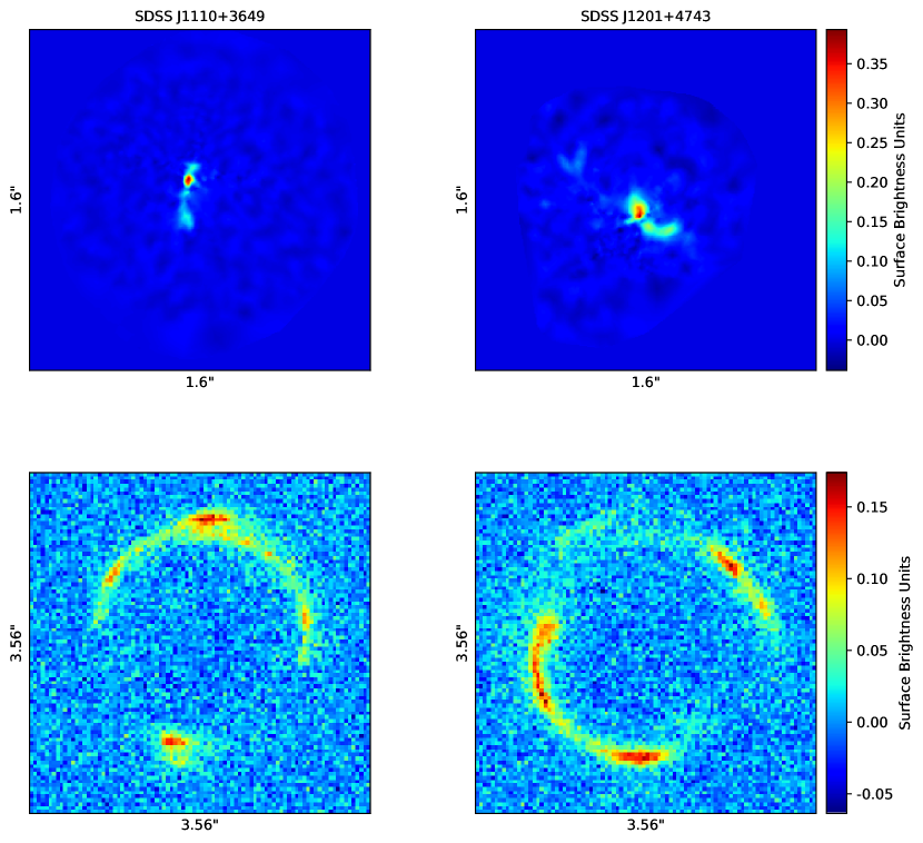
Figure 4: The left panel represents the system SDSS J1110+3649, and the right panel is for the system SDSS J1201+4743. On each side, the top Fig. represents the input source and the bottom Fig. gives the image after ray-tracing, convolving with an HST-type point spread function, and adding a noise corresponding to the noise of the HST observations. All figures share the same colour bar in units of surface brightness.

We create mock lensing observations based on two strong gravitational lens systems from the eBOSS Emission-Line Lens Survey for GALaxy-Ly$\alpha$ EmitteR sYstems (BELLS GALLERY, Shu et al. (2016a)): SDSSJ1110+3649 and SDSSJ1201+4743. We choose these specific systems because they have been studied in detail in previous works and have a reasonably good signal-to-noise level (Despali et al., 2019). They were observed with the WFC3-UVIS camera and the F606W filter on the Hubble Space Telescope. These systems have been independently modelled by Shu et al. (2016b), Nightingale et al. (2023) and Ritondale et al. (2018), and we use the lens model parameters from the latter. Observational details on the base systems are given in Tab. 2. Technical details are also provided in this table, where the Einstein radii are from Ritondale et al. (2019). We create mock observations that reproduce the original HST observations in terms of resolution and noise by convolving the obtained map with an HST-type point-spread function and adding a random noise field. The noise level of this field is obtained by Gaussian sampling at each pixel with a maximum value smaller by two orders of magnitude compared to the maximum brightness of the image, leading to a signal-to-noise ratio of $\frac{S}{N}=10$ and a standard deviation of the noise field ten times lower than the signal. The noise maps for the unperturbed and perturbed maps of the same system are computed independently. These two systems are presented in Fig. 4 with the respective image and source associated to each system.

Table 2: Summary of the image acquisition characteristics, and source and lens redshifts of both gravitationally lensed systems studied in this work, with the source and lens redshifts $z_{s}$ and $z_{l}$, rest-frame UV emission $\lambda_{r}$, and Einstein radius $R_{e}$. SDSSJ1201+4743 has two Einstein radii as the lens has two components.

Characteristic	SDSSJ1110+3649	SDSSJ1201+4743
Instrument	HST/WFC3-UVIS	-
Filter	F606W	-
Exp time [s]	2540	2624
Field of view [”2]	3.56$\times$3.56	-
Pixel size	90$\times$90	-
$z_{\rm l}$	0.733	0.563
$z_{\rm s}$	2.502	2.126
$\lambda_{\rm r}$ [Å]	1682	1883
$R_{\rm e}$ [”]	1.04 ± 0.02	1.72 ± 0.04
		0.94 ± 0.03

We build upon these systems to create three datasets: $\mathcal{D}_{1}$ and $\mathcal{D}_{2}$ based on SDSSJ1110+3649 and $\mathcal{D}_{3}$, based on SDSSJ1201+4743. Each dataset contains three variations:

• a mock image created from the lens parameters and best source with no additional perturbation (”Unperturbed”),

• a mock image where perturbations in the lens plane from simulated 1 keV WDM filaments and walls (”1 keV”) are added to the smooth case,

• an image with perturbations in the lens plane from simulated 3 keV WDM filaments and walls (”3 keV”).

We include the WDM perturbations to the deflection angles through the convergence maps described in the previous section. These are computed from a subregion of the full projected non-halo density maps. This subregion, marked by the white cross in Fig. 2, is chosen to have the highest density and thus maximises the perturbative effect of the non-halo structures. Although this does not allow for a statistical study, we perform a quantitative estimation of the effect of the non-halo structures and make sure that our conclusions are not taken from particular geometry or alignment effects in the chosen projections. More details about this are given in Sect. 5. The computed deflection angles are then added to the ones from the elliptical power-law lenses modelled in Ritondale et al. (2019) for the two systems of interest, and the brightness distribution from the corresponding source is propagated towards the observed plane through the lens plane and potential additional perturbations. The perturbations from the simulated non-halo 1 keV and 3 keV dark matter structures on the left column of Fig. 3 are the same for $\mathcal{D}_{1}$ and $\mathcal{D}_{3}$, and they have been rotated by 90 degrees for $\mathcal{D}_{2}$ to check that our results are not biased by a particular alignment or anti-alignment of the filaments/walls with intrinsic geometries of the lens mass model. Similarly, $\mathcal{D}_{3}$ is used to check that the results obtained with $\mathcal{D}_{1}$ are not from particular assets of the base system.

4 Lens modelling

To quantify the effect of non-halo structures, we model the mock data sets described above using the pronto code (Vegetti et al. in prep), a grid-based Bayesian modelling technique developed by Vegetti & Koopmans (2009), and further extended by Ritondale et al. (2019), Rizzo et al. (2018), Powell et al. (2020) and Ndiritu et al. (2024). We simultaneously infer the most probable parameters of the lens mass density distribution, $\boldsymbol{\eta_{m}}$, along with the brightness distribution and smoothness of the background source. The latter is modelled pixel by pixel in a regularised way, for the former, we assume an elliptical power-law profile (Bourassa & Kantowski, 1975; Bray, 1984; Kormann et al., 1994) given by

$$\kappa(x,y)=\frac{\kappa_{0}(2-\frac{\gamma}{2})q^{\gamma-3/2}}{2(q^{2}(x^{2}+r_{c}^{2})+y^{2})^{(\gamma-1)/2}},$$ (8)

where $\kappa_{0}$ is the surface mass density normalisation, $q$ is the axis ratio, $\gamma$ is the radial slope of the mass-density profile, and $r_{c}$ is the core radius, which is not a free parameter and is kept at $10^{-4}$ arcseconds. Two additional parameters account for external shear: the shear strength $\Gamma$ and the shear angle $\Gamma_{\theta}$. Finally, multipoles can be added as an extension to the elliptical power law + external shear profile. Here, we will use multipoles of the $3^{rd}$ order or of the $3^{rd}$ and $4^{th}$ orders. Multipoles of order $m$ create a convergence $\kappa_{m}$ of the form

$$\kappa_{m}(r,\phi)=r^{1-\gamma}[a_{m}\sin(m\phi)+b_{m}\cos(m\phi)],$$ (9)

where r and $\phi$ are the polar coordinates in the reference frame of the lens. These multipoles introduce asymmetries in the lens geometry, and one can probe their ability to absorb the perturbations of external massive components (O’Riordan & Vegetti, 2024; Powell et al., 2022). Therefore, the most extensive form of the free parameter vector is $\boldsymbol{\eta_{m}}=(\kappa_{0},q,\gamma,x_{c},y_{c},\theta,\Gamma,\Gamma_{\theta},a_{3},b_{3},a_{4},b_{4})$ with $x_{c}$, $y_{c}$, and $\theta$ the coordinates of the centre and the orientation of the lens. The values of the fiducial parameters used to create the mock data and the prior probability distributions are given in Tables 3 and 4.

Table 3: Values of the lens mass distribution fiducial parameters used to create the mock data and prior probability distributions to model it for $\mathcal{D}_{1}$ and $\mathcal{D}_{2}$. All the priors are uniform and cover a reasonably large range of values around the fiducial value.

Parameter ($\mathcal{D}_{1}$, $\mathcal{D}_{2}$)	Value	Prior
$\kappa_{0}$	1.14	$\mathcal{U}[1.0,1.4]$
$q$	0.82	$\mathcal{U}[0,1]$
$\gamma$	0.51	$\mathcal{U}[0,1]$
$x_{c}$	0.02	$\mathcal{U}[0.0,0.2]$
$y_{c}$	0.15	$\mathcal{U}[0.0,0.2]$
$\theta$	80.0	$\mathcal{U}[50,100]$
$\Gamma$	0	$\mathcal{U}[-0.05,0.05]$
$\Gamma_{\theta}$	0	$\mathcal{U}[-20,20]$
$a_{3}$	0	$\mathcal{U}[-0.02,0.02]$
$b_{3}$	0	$\mathcal{U}[-0.02,0.02]$
$a_{4}$	0	$\mathcal{U}[-0.02,0.02]$
$b_{4}$	0	$\mathcal{U}[-0.02,0.02]$

Table 4: Values of the lens mass distribution fiducial parameters used to create the mock data and prior probability distributions to model it for $\mathcal{D}_{3}$. All the priors are uniform and cover a reasonably large range of values around the fiducial value.

Parameter ($\mathcal{D}_{3}$)	Value	Prior
$\kappa_{0}$	1.19	$\mathcal{U}[1.0,1.4]$
$q$	0.78	$\mathcal{U}[0,1]$
$\gamma$	0.47	$\mathcal{U}[0,1]$
$x_{c}$	-0.13	$\mathcal{U}[-0.2,0]$
$y_{c}$	-0.18	$\mathcal{U}[-0.2,0]$
$\theta$	38.5	$\mathcal{U}[0,50]$
$\Gamma$	-0.01	$\mathcal{U}[-0.05,0.05]$
$\Gamma_{\theta}$	41.2	$\mathcal{U}[-10,50]$
$a_{3}$	0	$\mathcal{U}[-0.02,0.02]$
$b_{3}$	0	$\mathcal{U}[-0.02,0.02]$
$a_{4}$	0	$\mathcal{U}[-0.02,0.02]$
$b_{4}$	0	$\mathcal{U}[-0.02,0.02]$

Table 5: Values of the differences in logarithmic evidence from the nested sampling of the parameters of each model of lens mass distribution for $\mathcal{D}_{1}$, in the cases of the Unperturbed system, and the system with additional perturbations from the 1 keV and 3 keV simulations non-halo material. In each column, we compare three of our models with the reference one, where $\Delta_{0}$ is the reference logarithmic evidence value, and positive values indicate lower evidences for the more complex models.

$\Delta$log($\mathcal{E}$)	Unperturbed	1 keV	3 keV
Reference	$\Delta_{0}$	$\Delta_{0}$	$\Delta_{0}$
Fixed $\Gamma_{\theta}$,$\Gamma$	0.3±0.3	4.0±0.3	1.5±0.3
Multipoles $m=3$	21.5±0.3	15.6±0.3	34.3±0.3
Multipoles $m=3,4$	26.5±0.3	21.5±0.3	37.2±0.3

We explore the parameter space with the nested sampling algorithm MultiNest (Feroz et al., 2009). To compare two different models of the same dataset, we compare the logarithmic value of the evidence, log($\mathcal{E}$). A higher value of log($\mathcal{E}$) corresponds to a better fit of the model to the data, and therefore the difference $\Delta$log($\mathcal{E}$) = $\Delta_{0}$ - log($\mathcal{E}$) where $\Delta_{0}$ is a reference value - see Tab. 5 - is a quantitative way to compare the different models used for our systems. We consider four variations of the lens mass model:

• elliptical power law with free external shear used as a reference;

• elliptical power law with the external shear fixed to the best value from the previous case;

• elliptical power law with 3rd order multipoles;

• elliptical power law with 3rd and 4th order multipoles.

We fit each variation of the dataset $\mathbf{\mathcal{D}_{1}}$ (Unperturbed, 1 keV, 3 keV) with each of these mass models. In Tables 3 and 4, the priors are provided for all parameters. When a parameter is not included in the model, it is fixed at the fiducial value used to create the mock data. In the following, we will focus on this system as it is the most affected by the non-halo density perturbations. A complementary discussion, including the distributions for $x_{c}$, $y_{c}$, and $\lambda_{s}$ and the results for all three systems from $\mathcal{D}_{1}$ is given in Appendix A. In the case of $\mathcal{D}_{2}$ and $\mathcal{D}_{3}$, we only fit the simple power law + external shear model with the purpose of understanding possible biases in $\mathcal{D}_{1}$.

5 Results

(a)

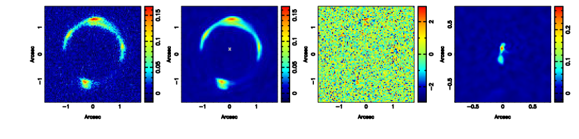
(b)

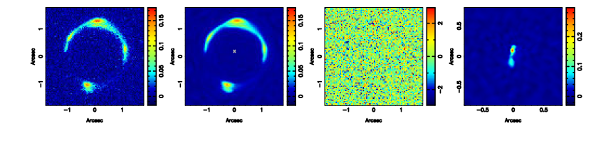
(c)

Figure 5: Optimisation results when modelling the three systems from $\mathcal{D}_{1}$ with an elliptical power law + external shear. The upper panel (a) shows the results for the Unperturbed system, the middle panel (b) for 1 keV, and the lower panel (c) for 3 keV. From left to right: images are the initial data, reconstructed model, normalised residuals between these two images, and reconstructed source. The units are arbitrary but are analogue to a 2D mass density

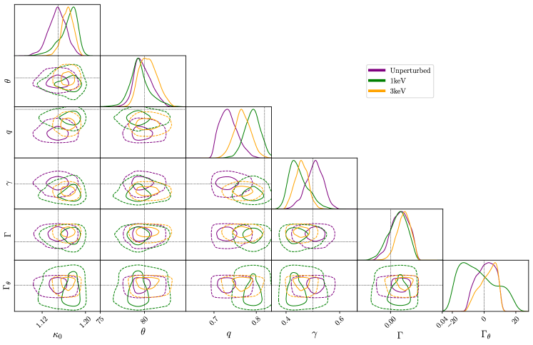
Figure 6: 1$\sigma$ and 2$\sigma$ contours for the parameters $\boldsymbol{\eta_{m}}$ (excluding the center coordinates $x_{c}$ and $y_{c}$, and the source regularisation $\lambda_{s}$) for the elliptical power law + external shear model of the Unperturbed, 1 keV and 3 keV systems in $\mathcal{D}_{1}$. The dashed lines show the 2D distributions, the solid lines show the marginal distributions and the dotted grey lines mark the true values.

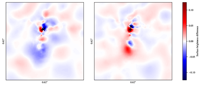
Figure 7: Difference in the sources brightness distribution in the source plane obtained when modelling the systems in $\mathcal{D}_{1}$ with a lens following an elliptical power law profile with additional external shear. If $S_{\text{X}}$ is the source mass distribution obtained for the system X, these images are the result of $S_{\text{Unperturbed}}-S_{\text{1 keV}}$ (left) and $S_{\text{Unperturbed}}-S_{\text{3 keV}}$ (right). Including more gravitational lensing effect under the form of additional perturbations and having these perturbations being absorbed in the main lens profile can shift and modulate the local surface brightness of the source. The general trend given by these images is that the main effect of the additional perturbation is an overall shift of the source, which is indicated by corresponding red and blue regions of the 2D brightness distribution. To highlight this effect, the black markers give the point of highest surface brightness (”+” for the unperturbed system, and ”x” for the perturbed one).

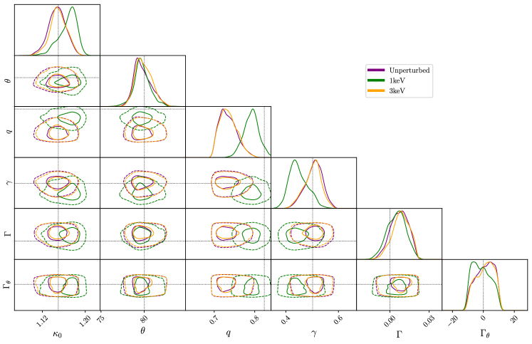
Figure 8: 1$\sigma$ and 2$\sigma$ contours for the parameters $\boldsymbol{\eta_{m}}$ for the elliptical power law + external shear model of the Unperturbed, 1 keV and 3 keV systems in $\mathcal{D}_{2}$. The layout is the same as in Fig. 6.

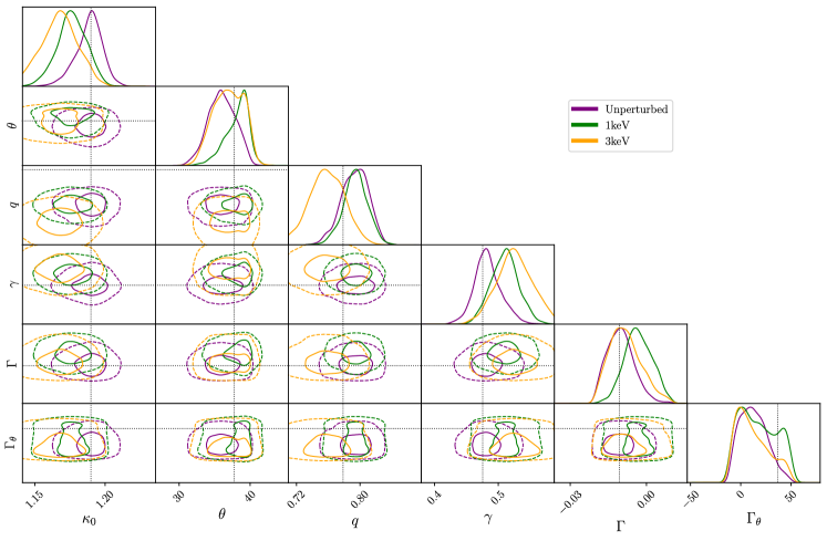
Figure 9: 1$\sigma$ and 2$\sigma$ contours for the parameters $\boldsymbol{\eta_{m}}$ for the elliptical power law + external shear model of the Unperturbed, 1 keV and 3 keV systems in $\mathcal{D}_{3}$. The layout is the same as in Fig. 6.

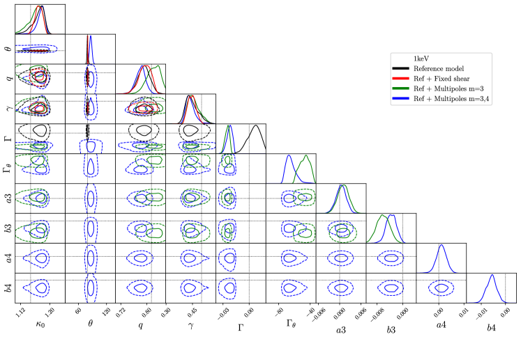
Figure 10: 1$\sigma$ and 2$\sigma$ contours for the parameters $\boldsymbol{\eta_{m}}$ (excluding the center coordinates $x_{c}$ and and $y_{c}$, and the source regularisation $\lambda_{s}$) for the four models of the 1 keV system in $\mathcal{D}_{1}$. The reference lens model is the elliptical power law + external shear.

In this section, we discuss the results of the lens modelling of mock images created with and without the inclusion of non-halo structures, as described in Sect. 4. For each dataset, we compare the evidence obtained by using the different mass models described in the previous section. The values of the evidence from the nested sampling are given in Tab. 5 for each model.

In this controlled experiment, we manually include the perturbations, as opposed to real observations where one does not know the underlying mass distribution of and around the main lens. We treat all the mock images as real observations and model them without imposing strong priors on the lens parameters. In this way, we want to test whether or not one is able to distinguish the effect of the non-halo structures from that of the main lens. In particular, one could expect their effect to appear as (or increase) the external shear, as this term is expected to represent the effect of the environment around the lens. Indeed, Etherington et al. (2023) show that the external shear term compensates for the lack of model complexity rather than describing sources of large-scale shear. Our mocks allow us to test this hypothesis in a controlled setting.

5.1 Are non-halo perturbations detected as external shear?

We begin by modelling the mock observations from the $\mathcal{D}_{1}$ set with the simplest lens model, which includes only a power-law profile and external shear. In all cases, this simple model is able to fit the data quite well, leaving no persistent structures in the residuals, which have mean and median values close to zero, even in the presence of the non-halo convergence. Fig. 5 shows the three mocks (first column) and the results of the lens modelling. The corresponding posterior distributions are shown in Fig. 6. If external shear describes the effect of large-scale structures, one would expect an increase (or variation) of the shear parameters in the perturbed case. Instead, we see that all lens parameters are affected, in particular the convergence normalisation, ellipticity $q$ and density slope $\gamma$. The posterior distribution for the shear strength $\Gamma$ and angle $\Gamma_{\theta}$ do not show a systematic difference compared to the unperturbed case, suggesting the orientation of the filaments and walls does not leave a distinctive imprint.

Overall, the changes in parameters’ posterior distributions are not significant, and the best-fit values for all the parameters remain sensibly the same within the 1$\sigma$ error bars. The perturbations, no matter their orientations along the line of sight, seem to be reabsorbed by a reasonably smooth (unperturbed) model in both the 1 keV and 3 keV cases. In fact, some of the differences in the mass model are absorbed by the source: as the source is pixelated and reconstructed at the same time as the lens model, the two are related and the sources react to changes in the lens model. The sources in the right column of Fig. 5 overall show the same shape and visually look similar and in very good agreement with the modelling from Ritondale et al. (2019). However, Fig. 7 shows that the differences between the resulting fine geometrical features and the source position shift lead to surface brightness differences up to half the maximum surface brightness of the source obtained for the Unperturbed system. As a check that the introduction of WDM perturbations does indeed shift the sources and does not alter the overall flux, we compute the ratio of integrated surface brightness $\frac{\Sigma S_{\text{1 keV}}}{\Sigma S_{\text{Unperturbed}}}$ and $\frac{\Sigma S_{\text{3 keV}}}{\Sigma S_{\text{Unperturbed}}}$ where the sums are done over all the map pixels, and which respectively yield 0.97 and 0.98. Previous works (Brainerd, 2001; Koopmans, 2005; Rau et al., 2013) have shown that small variations in the source structure can absorb the perturbations due to low-mass perturbations and thus prevent their detection. In this case, we see that the source can also absorb part of the effect of the extended convergence caused by the non-halo large-scale structures given that it does not visibly alter the surface brightness of the arc in a localised way.

We now model $\mathcal{D}_{2}$ and $\mathcal{D}_{3}$ to check if we get consistent results with the $\mathcal{D}_{1}$ analysis. Figs. 8 and 9 show the distribution of the posterior distributions for these two datasets. We remind the reader that $\mathcal{D}_{2}$ is generated from the same base system as $\mathcal{D}_{1}$ but with perturbations rotated by +90°. This is a good sanity check that our results for $\mathcal{D}_{1}$ do not emerge for specific alignments between the perturbations and other lens or source features. Comparing Figures 6 and 8 this gives us insights into the potential alignments between the source and the lens. Also in this case the values for most parameters lie in the same ranges within the uncertainties. This is a good qualitative indication that no parameter is strongly affected by the orientation of the perturbation. We can however appreciate some small differences: for $\mathcal{D}_{2}$, the parameters remain the same between the Unperturbed and the 3 keV systems and vary only when introducing the 1 keV perturbations, which are stronger. In $\mathcal{D}_{1}$, we instead see a gradual shift of the posterior distribution for $\kappa_{0}$, $q$ and $\gamma$ when perturbations are introduced. Given that the perturbation orientation is the only difference between the two cases, this indicates that in $\mathcal{D}_{2}$ the alignment with the lens can conspire to mask their effect - reabsorbing it into the model even more - in the 3 keV case as hinted by the convergence map in Fig. 3.

In $\mathcal{D}_{3}$ (Fig. 9), both the lens model and the input source are different. However, the effect of non-halo perturbation is of similar level than that already discussed for $\mathcal{D}_{1}$ and $\mathcal{D}_{2}$. This confirms that different perturbations alter the lenses, but that they remain in statistically good agreement with each other as all the 1$\sigma$ contours overlap.

5.2 Effect of lens model complexity

As discussed in the previous Section, the power-law + shear model is already a good fit to the data. However, we are interested in understanding which parameters are the most affected by the addition of non-halo structures, thus we test if the other models improve the evidence. We modelled $\mathcal{D}_{1}$ with four different mass models and thus can compare the resulting $\Delta$log($\mathcal{E}$) values displayed in Tab. 5 given that the same data are modelled with different mass models. As a first test, we fix the external shear parameters to the best value of the power-law + shear model. This reduces the number of parameters but decreases the quality of the lens modelling. The discrepancy between the evidence values gets bigger with the addition of non-halo perturbations, as $\Gamma$, even when it is consistent with 0 at the 1$\sigma$ level, can absorb some of these perturbation effects. We note that when $\Gamma$ is consistent with 0, the posterior distribution for the parameter $\Gamma_{\theta}$ does not converge as one cannot assign a meaningful direction to the sheer in this case (see Figures 10,  11, 12 and 13).

We then consider a mass model with additional complexity given by order 3 and 4 multipoles. The input lens mass model used to create the mock images does not contain multipoles, but one could think that multipoles would be preferred when adding the non-halo convergence. In each case (Unperturbed, 1 keV, 3 keV), the addition of multipoles (m=3 or m=3,4) to the model makes it worse and the evidence decreases ($\Delta$log($\mathcal{E}$) increases): the blue and green distributions of Fig. 10 shift away from the black and red ones, corresponding more to the input source, and are also broader, hence giving less precise constraints on the values of the parameters. Overall, the models with multipoles are less preferred and the posterior distributions of the parameters are less constrained, not accounting for the perturbations, although it is important to note that all multipoles parameters are consistent with 0 at the 1$\sigma$ level. Looking at the differences between the values of $\Delta$log($\mathcal{E}$) for all three systems, it could be tempting to assume that since they are lower in the 1 keV scenario, multipoles are better at absorbing 1 keV non-halo features than their 3 keV counterparts. However, one should not compare these three systems with each other, and we remind the reader that the perturbation introduced with the 1 keV and 3 keV simulations display different geometrical features.

Furthermore, looking at the distributions in Fig. 10, we can notice several similarities and differences between our four models for the 1 keV system (that are similar for the Unperturbed and 3 keV systems). Most parameters follow similar posterior distributions in different models within 1$\sigma$. For all the systems, it appears that every parameter’s posterior distribution converges. The Bayesian modelling used here (Vegetti & Koopmans, 2009) can provide optimised values for the lens profile in the four different types of models tested, and the presence of the perturbations is marked by minor shifts in the posterior distributions of the parameters. Thus, the perturbations introduced in the strong lensing signal by WDM non-halo structures appear as a systematic and are not equivalent to multipoles.

6 Conclusions

In this study, we have investigated if and to what extent the material outside of haloes, i.e. within filaments and walls, can cause statistically relevant and observable effects on gravitationally lensed arcs in the case of galaxy-galaxy lensing. Such effects could be used to constrain the dark matter particle mass (or, equivalently, warmth), and we tested the effects of non-halo material from two simulations of WDM cosmological scenarios with dark matter particle masses $m_{\chi}$ = 1 keV and $m_{\chi}$ = 3 keV. So far, most studies have focused on the effects of dark matter haloes on gravitationally lensed systems, but a recent study (Richardson et al. (2022), R22 in this work) has already shown the effects of such non-halo structures on quadruply-lensed quasars. Despite numerous simplifications, the authors show that in a $m_{\chi}=3$ keV scenario, neglecting the non-halo material can lead to an underestimation of the flux ratios by $5$ to $10$ per cent, while this number goes up to $50$ per cent for $m_{\chi}=1$ keV. Although this dark matter model is already observationally ruled out, the authors conclude that non-halo material should be included in rigorous models and that their inclusion can lower the constraints on the dark matter particle mass, allowing for the more permissive study of cosmologies.

We have used WDM $N$-Body simulations with $m_{\chi}=3$ keV and $m_{\chi}=1$ keV as in R22. These are novel fragmentation-free simulations, where particles are classed in four classes : voids, pancakes, filaments, and halos. $256^{3}$ particles are used to build the density field, and $512^{3}$ additional particles are used to reconstruct the high resolution density field in collapsed structures where interpolation fails. From the simulated density fields, we obtain non-halo structures convergence maps that we add as perturbations to two gravitationally lensed systems from the BELLS-Gallery. We have proposed four different models for the lens mass distribution of the systems in a first dataset and completed this step with one model of each system in a second and a third dataset. Classic lens models describe the main lens with a single elliptical power-law (with or without additional multipoles), while the contribution of matter on larger scales is represented by an external shear term. Our simulated observations allow us to test whether or not this term actually corresponds to extended mass components, such as filaments and walls, and if they can be distinguished from the main lens model. Our main conclusions are:

• Of all tested models we find that a single elliptical power-law deflector with additional external shear provides the best fit. Removing external shear or adding multipoles does not help to account for the potential effects of non-halo structures. In fact, all multipole parameters are consistent with 0 at the 1$\sigma$ level.

• When jointly reconstructing the lens and source, WDM perturbations are absorbed by the model parameters but introduce a systematic bias into both the lens surface brightness distribution and the lens mass-density distribution. The main effect on the reconstructed source is small localised displacements while there appears to be no particular global modulation of the shape and surface brightness of the sources.

• Regarding the lens model parameters, we find that the commonly used singular elliptical power-law lens + external shear parametrisation is sufficient to account for most of the effect at the cost that these perturbers cannot be distinguished from others that are also absorbed by this parametrisation (Despali et al., 2021).

The simulated WDM non-halo material studied in this work originates from the same simulations as in R22, thus we have to take the same precautions as them when interpreting our results, and our limitations are of similar natures: we used the thin-lens approximation, baryonic effects are not modelled, dark matter particles of such warmth are already observationally excluded, and the line of sight is relatively short (80$h^{-1}$Mpc) compared to typical gravitationally lensed systems sizes. Thus, it is not possible to thoroughly quantify the effect of the non-halo structures of the line of sight, and we only consider their relative effects in the region of the main lens.

We conclude that in the case of galaxy-galaxy lensing, the effects of filaments and walls, i.e. material outside of haloes, impacts the reconstruction of the source surface brightness in a non-trivial way when using common lens mass profiles, but remains negligible in WDM cosmologies with $m_{\chi}$=1 keV and $m_{\chi}$=3 keV, and therefore for colder cosmologies too, where the relative importance of non-haloes compared to the one of haloes is lower.

Appendix A Details on the System Modelling

Figures 11, 12 and 13 give the posterior distributions for all the lens parameters used to model the three systems in $\mathcal{D}_{1}$.

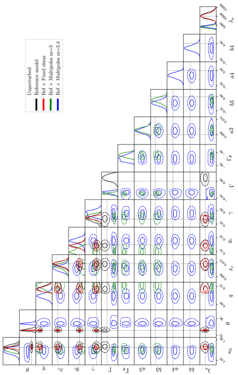
Figure 11: 1$\sigma$ and 2$\sigma$ contours for the parameters $\boldsymbol{\eta_{m}}$ and $\lambda_{s}$ for the four models of the Unperturbed system in $\mathcal{D}_{1}$.

Figure 12: 1$\sigma$ and 2$\sigma$ contours for the parameters $\boldsymbol{\eta_{m}}$ and $\lambda_{s}$ for the four models of the 1 keV system in $\mathcal{D}_{1}$.

Figure 13: 1$\sigma$ and 2$\sigma$ contours for the parameters $\boldsymbol{\eta_{m}}$ and $\lambda_{s}$ for the four models of the 3 keV system in $\mathcal{D}_{1}$.