Lyapunov exponents as probes for phase transitions of Kerr-AdS black holes

Abstract

In this paper, we study proper time Lyapunov exponents and coordinate time Lyapunov exponents of chaos for both massless and massive particles orbiting four-dimensional and five-dimensional Kerr-AdS black holes, and explore their relationships with phase transitions of these black holes. The results reveal that these exponents can reflect the occurrence of phase transitions. Specifically, when compared to the Lyapunov exponents of massive particles in chaotic states, the exponents corresponding to massless particles demonstrate a more robust capability in describing the phase transitions. Furthermore, we conduct a study on critical exponents associated with the Lyapunov exponents in these black holes, identifying a critical exponent value of 1/2.

1 Introduction

The motions of particles in the vicinity of black holes(BHs) has garnered significant attention, as these motions convey important information about their background spacetimes. Specifically, particles possess an innermost stable circular orbit around a BH, and once they cross this critical threshold, they are inevitably swallowed by the BH PQR ; LLL ; ZWSYL ; ZL . The radius of this orbit is contingent upon the BH’s mass and rotational velocity, thereby serving as a reflection of its spacetime geometry. Furthermore, the study of these orbits provides valuable insights into accretion disks and associated radiation spectra PT .

The unique physical properties and spacetime structures of BHs can induce instability in the geodesics of particles orbiting them. Compared to stable geodesics, these unstable geodesics possess greater observational value. BHs’ shadows are cast by combined effects of their event horizons’ capture of photons and strong gravitational lensing effect EHT1 ; EHT2 ; EHT3 ; EHT4 . By observing these shadows, one can deduce fundamental attributes such as the mass and rotation of the BHs, as well as the physical characteristics of their surrounding environments, thereby constraining related physical parameters. Furthermore, observations of BH shadows hold potential for shedding light on BH mergers. When disturbed by external fields, BHs evolve and propagate outward in the form of quasinormal modes(QNMs). The vibration frequencies and decay times of these QNMs are governed by the BHs’ characteristic parameters, including their masses, charges and angular momenta. Null geodesics serve as important tools for acquiring these QNMs RAK . Specifically, the angular velocities at the unstable null geodesics orbits determine the real parts of the QNMs, whereas their imaginary parts are associated with the unstable time scales of the orbits. Notably, the dominant modes can be observed in the gravitational wave signals emitted by BHs BPA1 ; BPA2 ; BPA3 . Optical appearances of stars undergoing gravitational collapse largely depend on the circular unstable null geodesics, which also explain the exponential fade-out of the luminosity of the collapsing stars AT . For some unstable geodesics, even slight disturbances can trigger chaotic motion of particles. This chaotic signature would leave an imprint on gravitational waves emitted from BHs KT1 ; KT2 ; KT3 ; KT4 ; KT5 ; KT6 . Therefore, the study of unstable geodesics around BHs not only provides insights into the fundamental properties of BHs but also offers potential observational signatures that can be detected through gravitational wave observations and other astronomical phenomena.

On the other hand, the exploration of phase transitions in BHs originated with the revelation of the Hawking-Page phase transition SWHP . Following the interpretation of the cosmological constant in anti-de Sitter (AdS) spacetimes as pressure, a series of works unveiled striking similarities between BHs and fluids in the context of phase transitions AA1 ; AA2 ; AA3 ; AA4 ; AA5 ; AA6 ; AA7 ; AA8 ; AA9 ; AA10 ; BB1 ; BB2 ; BB3 ; BB4 ; BB5 ; BB6 ; BB7 ; BB8 ; BB9 ; BB10 ; CC1 ; CC2 ; CC3 ; CC4 ; CC5 ; CC6 . During these phase transitions, the BHs parameters change, which can directly impact on the physical environment surrounding them. This alteration in physical environment may trigger the occurrence of chaos among the particles. Furthermore, the chaos of particles around BHs may subtly alter the states of the systems, which can accumulate and eventually trigger phase transitions. Consequently, there exists a close connection between the chaos and phase transitions, where the chaotic behaviors of particles can reflect the phase transitions in the systems. In light of this connection, the Lyapunov exponent(LE) in terms of coordinate time associated with the chaotic behavior of the particles and ring strings around the Reissner-Nordström-AdS BH was researched in GLMW . The study revealed that the exponent exhibits multiple values when a phase transition occurs. The discontinuous change in the exponent was considered as an order parameter, and a relationship between this exponent and the critical temperature was established, yielding a critical exponent of 1/2. Subsequently, this work was extended to other spherically symmetric spacetimes YTMH ; LTW ; KPA ; DLMG ; SDDM ; GAP . These studies provide novel insights into the understanding of phase transitions.

In this paper, we study proper time Lyapunov exponents(PTLEs) and coordinate time Lyapunov exponents(CTLEs) of chaotic motion exhibited by massless and massive particles around four-dimensional and five-dimensional Kerr-AdS BHs, and explore their relationships with phase transitions of these BHs. For the four-dimensional case, we fix the particles’ angular momenta and calculate the critical value of the rotational parameter at the phase transition point. Building upon this foundation, we further examine these relationships under scenarios where the parameter falls below its critical threshold. Furthermore, we compute the critical exponents which are related to these LEs. For the five-dimensional Kerr-AdS BH with two rotational parameters, we fix the angular momenta of the particles’ and one of the rotational parameters to study the PTLE and CTLE. This allows us to further explore their relationships with the phase transition.

The remainder of this paper is organized as follows. In the subsequent section, we review the acquisition of the PTLE and CTLE. In Section 3, we study the phase transition of the four-dimensional Kerr-AdS BH, exploring its relationship with the PTLEs and CTLEs of both massless and massive particles in their chaotic motion. Furthermore, we calculate the critical exponents associated with both the CTLEs and PTLEs. In Section 4, our study is extended to the five-dimensional Kerr-AdS BH, where we continue to explore the connection between its phase transition and the PTLEs and CTLEs exhibited by particles in chaotic motion. The final section is devoted to our conclusions and discussions.

2 Review of LEs

LEs serve as significant indicators for quantifying chaotic characteristics, as they characterize the average exponential rates at which adjacent orbits in the phase space of classical systems either converge or diverge. A positive LE signifies divergence between two neighboring geodesics, thereby indicating that the system is highly sensitive to initial conditions, potentially leading to chaotic behavior. Conversely, a negative exponent implies a tendency towards stability within the system. When the exponent is zero, the system exhibits periodic motion. In this section, we first review the acquisition of both the PTLE and CTLE CMBWZ ; PP1 ; PP2 ; PP3 ; LG1 ; LG2 ; GCYW .

For a particle in equilibrium outside a BH, its equation of motion can be schematically represented as follows

$$\frac{dX_{i}}{dt}=F_{i}(X^{j}),$$ (1)

where $X_{i}$ are coordinates and $F_{i}(X^{j})$ are functions to be determined. We linearise the above equations around a certain orbit and get

$$\frac{d\delta X_{i}(t)}{dt}=K_{ij}(t)\delta X_{j}(t),$$ (2)

where $K_{ij}(t)$ is a Jacobian matrix defined by

$$K_{ij}(t)=\left.\frac{\partial F_{i}}{\partial X_{j}}\right|_{X_{i}(t)}.$$ (3)

When the particle moves in an circular orbit with radius $r_{0}$ on the equator of the black hole, we define the classical phase space variables $X_{i}(t)=(p_{r},r)$. Evidently, such an orbit can exist in spherically symmetric spacetimes or in the equatorial planes of axisymmetric spacetimes CMBWZ . Utilizing the canonical momenta, given by $p_{q}=\frac{\partial\mathcal{L}}{\partial\dot{q}}$, and the Euler-Lagrange equations of motion

$$\frac{dp_{q}}{d\tau}=\frac{\partial\mathcal{L}}{\partial q},$$ (4)

we get $\frac{dp_{r}}{d\tau}=\frac{\partial\mathcal{L}}{\partial r}$ and $\frac{dr}{d\tau}=\frac{p_{r}}{g_{rr}}$. Consequently, the matrix is obtained as

$$K_{ij}=\begin{pmatrix}0&\frac{d}{dr}\left(\frac{\partial\mathcal{L}}{\partial r}\right)\\ \frac{1}{g_{rr}}&0\end{pmatrix}.$$ (5)

The exponent is determined by the eigenvalues of the Jacobian matrix evaluated at the equilibrium point, which are obtained as follows

$$\lambda^{2}_{p}=\frac{1}{g_{rr}}\frac{d}{dr}\left(\frac{\partial\mathcal{L}}{\partial r}\right),$$ (6)

To further derive its expression, we utilize Lagrange’s equation of geodesic motion

$$\frac{d}{d\tau}\left(\frac{\partial\mathcal{L}}{\partial\dot{r}}\right)-\frac{\partial\mathcal{L}}{\partial r}=0,$$ (7)

and the formula

$$\frac{d}{d\tau}\left(\frac{\partial\mathcal{L}}{\partial\dot{r}}\right)=\frac{d}{d{\tau}}(g_{rr}\dot{r})=\frac{1}{2g_{rr}}\frac{d}{dr}(g_{rr}^{2}\dot{r}^{2}).$$ (8)

Thus the expression of $\frac{\partial\mathcal{L}}{\partial r}$ is gotten

$$\frac{\partial\mathcal{L}}{\partial r}=\frac{1}{2g_{rr}}\frac{d}{dr}(g_{rr}^{2}\dot{r}^{2}).$$ (9)

After defining an effective potential as $V_{r}=\dot{r}^{2}$, we substitute this formula into Eq. (6). Taking into account an unstable equilibrium orbit, we find that $V_{r}=V^{\prime}_{r}=0$, where the prime denotes the derivative with respect to $r$. Consequently, the exponent is obtained as outlined below

$$\lambda_{p}=\sqrt{\frac{V^{\prime\prime}_{r}}{2}},$$ (10)

which is defined as the PTLE. On the other hand, from the Euler-Lagrange equations of motion, we have $\frac{dp_{r}}{dt}=\frac{d\tau}{dt}\frac{\partial\mathcal{L}}{\partial r}$. Thus the exponent in term of coordinate time is expressed as

$$\lambda_{c}=\sqrt{\frac{V^{\prime\prime}_{r}}{2\dot{t}^{2}}},$$ (11)

which is defined as the CTLE. These two exponents reflect the stability of the motion of equatorial particles in the spherical spacetimes and in the equatorial planes of the axisymmetric spacetimes. Their relationship is expressed by $\lambda_{p}=|\dot{t}|\lambda_{c}$. Since $|\dot{t}|>0$, their properties are closely related in the spherically symmetric spacetimes LG2 .

3 LEs and phase transitions of four-dimensional Kerr-AdS BHs

3.1 Thermodynamics of four-dimensional Kerr-AdS BHs

The Kerr-AdS BH is a vacuum solution of Einstein field equations characterized by a negative cosmological constant. It describes a rotational AdS spacetime and its metric is given by

$$ds^{2}=-\frac{\Delta}{\rho^{2}}\left(dt-\frac{a\sin^{2}\theta}{\Xi}d\varphi\right)^{2}+\frac{\rho^{2}}{\Delta}dr^{2}+\frac{\rho^{2}}{\Sigma}d\theta^{2}+\frac{\Sigma\sin^{2}\theta}{\rho^{2}}\left[adt-\frac{(r^{2}+a^{2})}{\Xi}d\varphi\right]^{2},$$ (12)

with the metric functions

$$\Delta = \left(r^{2}+a^{2}\right)\left(1+\frac{r^{2}}{l^{2}}\right)-2mr,\quad\Xi=1-\frac{a^{2}}{l^{2}},$$

$$\rho^{2} = r^{2}+a^{2}\cos^{2}\theta,\quad\Sigma=1-\frac{a^{2}}{l^{2}}\cos^{2}\theta.$$ (13)

where $m$, $a$ and $l$ are the mass parameter, rotational parameter and AdS radius, respectively. $l$ is related to the cosmological constant as $\Lambda=-3l^{2}$. The AdS radius and rotational parameter obey a relation $a^{2}<l^{2}$. When $a^{2}=l^{2}$, the metric is singular. The ADM mass is $M=\frac{m}{\Xi^{2}}$ and the angular momentum is $J=\frac{ma}{\Xi^{2}}$. The entropy and Hawking temperature are

$$S = \frac{\pi(r_{+}^{2}+a^{2})}{\Xi},$$ (14)

$$T = \frac{3r_{+}^{4}+r_{+}^{2}(a^{2}+l^{2})-a^{2}l^{2}}{4\pi l^{2}r_{+}(r_{+}^{2}+a^{2})},$$ (15)

where $r_{+}$ is the event horizon determined by the largest positive root of $\Delta=0$. At the horizon, the angular velocity is

$$\Omega_{+}=\frac{a(r_{+}^{2}+l^{2})}{l^{2}(r_{+}^{2}+a^{2})}.$$ (16)

In the extended phase spaces, the cosmological constant is treated as a variable to pressure, while the mass is regarded as enthalpy. The phase transition of this BH has been discussed in AKMS1 ; AKMS2 ; YZWL1 ; YZWL2 . In these studies, the pressure is defined as $P=\frac{3}{8\pi l^{2}}$, and the conjugate thermodynamic volume is $V=\frac{4\pi(r_{+}^{2}+a^{2})}{3\Xi}\left[\frac{(r_{+}^{2}+l^{2})a^{2}}{2r_{+}^{2}\Xi l^{2}}+1\right]$. For a fixed cosmological constant, the aforementioned thermodynamic variables adhere to the first law of BH thermodynamics

$$dM=TdS+\Omega_{+}dJ.$$ (17)

The Gibbs free energy for the BH is

$$F=M-TS=\frac{(r_{+}^{2}+a^{2})(r_{+}^{2}+l^{2})}{2\Xi^{2}l^{2}r_{+}}-\frac{3r_{+}^{4}+r_{+}^{2}(a^{2}+l^{2})-a^{2}l^{2}}{4\Xi l^{2}r_{+}}.$$ (18)

Through dimensional analysis, we observe that certain physical quantities scale as powers of $l$ and they can be written as follows

$$r=\bar{r}l,\quad r_{+}=\bar{r}_{+}l,\quad a=\bar{a}l,\quad m=\bar{m}l,\quad T=\bar{T}l^{-1},\quad F=\bar{F}l.$$ (19)

where $\bar{r}$, $\bar{r}_{+}$, $\bar{a}$, $\bar{m}$, $\bar{T}$ and $\bar{F}$ are all dimensionless quantities. Eq. (15) demonstrates that the temperature $T$ is a function of $r_{+}$. By utilizing this equation in conjunction with Eq. (48), we can derive a function $\bar{r}_{+}(\bar{T})$. When a specific value of $\bar{T}$ corresponds to multiple values of $\bar{r}_{+}$, it signifies that the BH possesses multiple phases. Conversely, when this is not the case, the BH displays only a single phase. This relationship is depicted in Figure 1, where $\bar{a}_{c}=0.124553$ represents the value at a critical point and is determined by

$$\frac{\partial\bar{T}}{\partial\bar{r}_{+}}=\frac{\partial^{2}\bar{T}}{\partial\bar{r}_{+}^{2}}=0.$$ (20)

The other critical values are $\bar{r}_{+}=0.384471$ and $\bar{T}=0.253635$. In Figure 1, it is observed that there is no inflection point, and the temperature increases monotonically for $\bar{a}=0.14$. This indicates that each phase is uniquely associated with a single temperature value. Conversely, when $\bar{a}<\bar{a}_{c}$, inflection points appear, suggesting that the BH exhibits multiple phases for a given value of $\bar{T}$. Specifically, for $\bar{a}=0.05$ and $\bar{T}=\bar{T}_{0}$, there exist three roots: $\bar{r}_{1+}$, $\bar{r}_{2+}$ and $\bar{r}_{3+}$, which correspond to three phases of small, intermediate and large BHs, respectively.

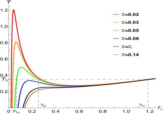
Figure 1: The temperature of the four-dimensional Kerr-AdS BH varies as a function of the horizon radius.

To further elucidate the phase transition, we present the curves depicting the free energy as a function of the temperature in Figure 2. In Figure 2, the absence of a swallowtail-like structure for $\bar{a}=0.14$ indicates the absence of a phase transition. Conversely, when $\bar{a}<\bar{a}_{c}$, swallowtail-like structures emerge, typically signaling the onset of a phase transition between large and small BHs. Figure 2 specifically illustrates the change in free energy at $\bar{a}=0.02$. Here, the free energy monotonically decreases for $\bar{T}<\bar{T}_{1}$ and $\bar{T}>\bar{T}_{3}$. A small BH phase is observed for $\bar{T}<\bar{T}_{1}$, while a large BH phase appears for $\bar{T}>\bar{T}_{3}$. In both cases, the BHs are stable. Within the range $\bar{T}_{1}<\bar{T}<\bar{T}_{3}$, the free energy becomes multivalued, with small, intermediate and large BHs coexisting. These phases transform into each other within this temperature range. The first-order phase transition between a small and large BH occurs at $\bar{T}_{3}$.

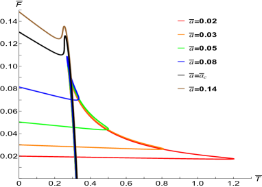
(a)

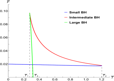
(b)

Figure 2: The free energy of the four-dimensional Kerr-AdS BH varies with the temperature. The scenario where $\bar{a}=0.02$ is illustrated in Figure 2.

3.2 LEs and phase transitions

The motions of particles outside BHs can reflect certain characteristics of the background spacetimes in which the particles reside. In this section, we study the thermodynamic phase transition of the four-dimensional Kerr-AdS BH by examining the PTLE and CTLE associated with the chaotic motion of both massless and massive particles.

When a neutral particle moves in the equatorial plane of the BH, its Lagrangian is given by

$$\mathcal{L}=\frac{1}{2}g_{\mu\nu}\dot{x}^{\mu}\dot{x}^{\nu}=\frac{1}{2}\left(\bar{g}_{tt}\dot{t}^{2}+\bar{g}_{rr}\dot{r}^{2}+\bar{g}_{\varphi\varphi}\dot{\varphi}^{2}+2\bar{g}_{t\varphi}\dot{t}\dot{\varphi}\right).$$ (21)

Here we use $\bar{g}_{\mu\nu}$, where $\mu,\nu=t,r,\varphi$, to represent the components of the Kerr-AdS metric in the equatorial plane ($\theta=\frac{\pi}{2}$). Dots are employed to denote derivatives with respect to the proper time. The specific expressions for $\bar{g}_{\mu\nu}$ are

$$\bar{g}_{tt}=-\frac{\Delta-a^{2}}{r^{2}},\quad\bar{g}_{rr}=\frac{r^{2}}{\Delta},\quad\bar{g}_{\varphi\varphi}=\frac{(r^{2}+a^{2})^{2}-\Delta a^{2}}{r^{2}\Xi^{2}},\quad\bar{g}_{t\varphi}=-\frac{(r^{2}+a^{2}-\Delta)a}{r^{2}\Xi}.$$ (22)

Using the definition of generalized momenta $p_{\mu}=\frac{\partial\mathcal{L}}{\partial\dot{x}^{\mu}}=g_{\mu\nu}\dot{x}^{\nu}$, we get

$$p_{t} = \bar{g}_{tt}\dot{t}+\bar{g}_{t\varphi}\dot{\varphi}=-E,$$ (23)

$$p_{r} = \bar{g}_{rr}\dot{r},$$ (24)

$$p_{\varphi} = \bar{g}_{\varphi\varphi}\dot{\varphi}+\bar{g}_{t\varphi}\dot{t}=L,$$ (25)

where $E$ and $L$ are the energy and angular momentum of the particle, respectively. From the above equations, it is straightforward to derive the equations governing $t$-motion and $\varphi$-motion,

$$\dot{t} = \frac{E\bar{g}_{\varphi\varphi}+L\bar{g}_{t\varphi}}{g_{t\varphi}^{2}-\bar{g}_{tt}\bar{g}_{\varphi\varphi}},$$ (26)

$$\dot{\varphi} = \frac{E\bar{g}_{t\varphi}+L\bar{g}_{tt}}{\bar{g}_{tt}g_{\varphi\varphi}-\bar{g}_{t\varphi}^{2}}.$$ (27)

The Hamiltonian of the system is

$$2\mathcal{H}=2(p_{\mu}\dot{x}^{\mu}-\mathcal{L})=p_{\mu}\dot{x}^{\mu}=\bar{g}_{tt}\dot{t}^{2}+\bar{g}_{rr}\dot{r}^{2}+\bar{g}_{\varphi\varphi}\dot{\varphi}^{2}+2\bar{g}_{t\varphi}\dot{t}\dot{\varphi}=\delta,$$ (28)

where $\delta=0$ and $-1$ correspond to null and time-like geodesics, respectively. Solving Eq. (28), we get $r$-motion

$$\dot{r}^{2}=\frac{\delta}{\bar{g}_{rr}}-\frac{E^{2}\bar{g}_{\varphi\varphi}+L^{2}\bar{g}_{tt}+2EL\bar{g}_{t\varphi}}{\bar{g}_{rr}(\bar{g}_{tt}\bar{g}_{\varphi\varphi}-\bar{g}_{t\varphi}^{2})}.$$ (29)

3.2.1 Null geodesic’s case

The motion of massless particles is governed by the null geodesic equations. By employing the definition of the effective potential, denoted as $V_{r}=\dot{r}^{2}$, we derive an expression for the effective potential of a massless particle within the context of Kerr-AdS spacetime,

$$V_{r}=\frac{(aE-L\Xi)^{2}\Delta-\left[E(r^{2}+a^{2})-aL\Xi_{a})\right]^{2}}{r^{4}}.$$ (30)

We initially determine the position of the unstable equilibrium orbit for the particle, which is governed by the conditions $V_{r}=V_{r}^{\prime}=0$ and $V_{r}^{\prime\prime}>0$. Subsequently, we study the relationship between the PTLE and CTLE of chaos for the particle at this orbit and the temperature. Utilizing Eqs. (10), (11) and (30), we obtain the PTLE and CTLE. Their variations with the temperature are illustrated in Figures 3 and 4, respectively. For the calculations presented in this paper, we adopt $L=20l$.

The variation of the PTLE with the temperature is depicted in Figure 3. Specifically, in Figure 3, the exponent decreases monotonically when $\bar{a}=0.14$, whereas it is a multivalued function with respect to $\bar{T}$ when $\bar{a}<\bar{a}_{c}$ (where $\bar{a}_{c}$ is defined in Section 3.1). Figure 3 illustrates the exponent’s variation with the temperature for the case when $\bar{a}=0.02$. Here, it decreases monotonically when $\bar{T}<\bar{T}_{1}$ and $\bar{T}>\bar{T}_{2}$, and assumes three values for a specific value of $\bar{T}$ within the range $\bar{T}_{1}<\bar{T}<\bar{T}_{2}$ (where $\bar{T}_{1}$ and $\bar{T}_{2}$ correspond exactly to the temperatures in Figure 2, respectively). The small and large BH branches emerge in the ranges $\bar{T}<\bar{T}_{1}$ and $\bar{T}>\bar{T}_{2}$ respectively, and they are stable. Between $\bar{T}_{1}$ and $\bar{T}_{2}$, the small, intermediate and large BH phases coexist, implying that they can transform into each other within this temperature range. The first order phase transition occurs at $\bar{T}_{3}$. These behaviors resemble those observed in Figure 2, thereby indicating that the PTLE serves as a probe for the phase transition of the four-dimensional Kerr-AdS BH.

Recently, Maldacena, Shenker and Stanford conjectured the existence of a universal upper bound on the exponent and this bound is related to the system’s temperature MSS . However, in this context, the exponent attains its maximum value at $\bar{T}=0$, which changes with the change in $\bar{a}$’s value. Therefore, our results suggest a violation of this bound LG2 ; GCYW ; LL1 ; LL2 ; LL3 .

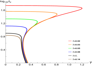
(a)

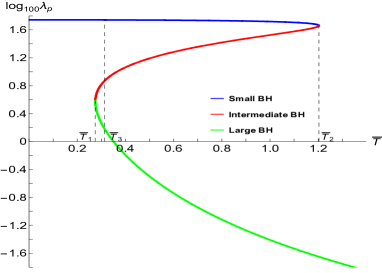
(b)

Figure 3: The variation of the PTLE of chaos for the massless particle, as a function of the temperature of the four-dimensional Kerr-AdS BH. The specific scenario with $\bar{a}=0.02$ is depicted in 3.

The curves in Figure 4 illustrates the variation of the CTLE with the temperature for different values of $\bar{a}$. In Figure 4, the exponent is a multivalued function when $\bar{a}<\bar{a}_{c}$, whereas it consistently assumes a single value for a specific temperature when $\bar{a}>\bar{a}_{c}$. As the temperature increases, the exponents for different values of $\bar{a}$ eventually converge, indicating a pronounced influence of the temperature on the exponent. The graph in Figure 4 depicts the trend of the exponent as it varies with the temperature when $\bar{a}=0.02$. It is evidently that, for a given temperature, the exponent is multivalued within the range $\bar{T}_{1}<\bar{T}<\bar{T}_{2}$ and single valued when $\bar{T}<\bar{T}_{1}$ and $\bar{T}>\bar{T}_{2}$. Within the range $\bar{T}_{1}<\bar{T}<\bar{T}_{2}$, two scenarios emerge: in the small and large BH branches, the exponent decreases with increasing $\bar{T}$, whereas it increases with increasing $\bar{T}$ in the intermediate BH branch. Comparison with Figure 2 reveals that the temperature region with multiple values of the exponent corresponds to the phase transition region depicted in Figure 2. In the large BH branch, where $\bar{T}>\bar{T}_{2}$, the exponent approaches $1$ as $\bar{T}$ continues to increase. Therefore, the CTLE also serves as a probe for the phase transition.

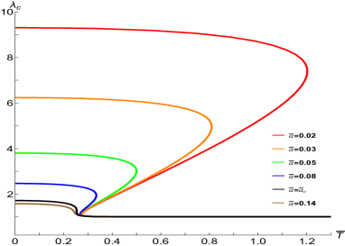
(a)

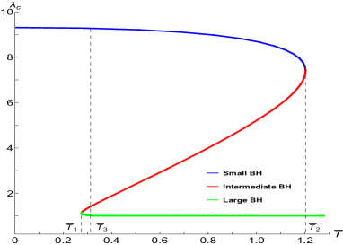
(b)

Figure 4: The variation of the CTLE of chaos for the massless particle, as a function of the temperature of the four-dimensional Kerr-AdS BH. The specific scenario with $\bar{a}=0.02$ is depicted in 4.

3.2.2 Timelike geodesic’s case

To explore the relationship between the phase transition and the PTLE of chaos for the massive particles, as well as its relationship with the CTLE, we undertake the calculation of the effective potential for such particles. Specifically, for a time-like geodesic, where $\delta=-1$, the corresponding effective potential is expressed as follows

$$V_{r}=\frac{-\Delta r^{2}+(aE-L\Xi)^{2}\Delta-\left[E(r^{2}+a^{2})-aL\Xi_{a})\right]^{2}}{r^{4}}.$$ (31)

Thus the position of the unstable equilibrium orbit for the massive particle is determined by solving the equations $V_{r}=V_{r}^{\prime}=0$ and $V_{r}^{\prime\prime}>0$. Subsequently, by utilizing Eqs. (10), (11) and (31), we obtain the PTLE and CTLE at this orbit. The variations of these quantities with the temperature are depicted in Figures 5 and 6, respectively.

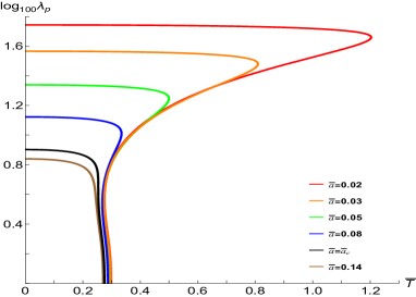
(a)

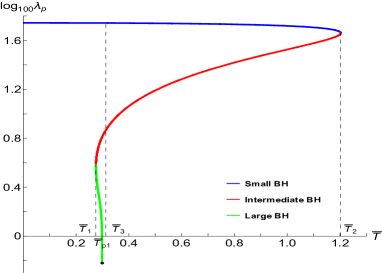
(b)

Figure 5: The variation of the PTLE of chaos for the massive particle, as a function of the temperature of the four-dimensional Kerr-AdS BH. The specific scenario with $\bar{a}=0.02$ is depicted in 5.

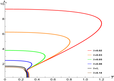
(a)

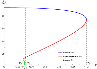
(b)

Figure 6: The variation of the CTLE of chaos for the massive particle, as a function of the temperature of the four-dimensional Kerr-AdS BH. The specific scenario with $\bar{a}=0.02$ is depicted in 6.

Figure 5 depicts the influence of the temperature on the PTLE for different values of $\bar{a}$. In Figure 5, we similarly observe that the exponent is a multivalued function when $\bar{a}<\bar{a}_{c}$, hinting at the presence of phase transitions. The scenario for $\bar{a}=0.02$ is illustrated in Figure 5, where $\bar{T}_{P1}$ signifies a terminal temperature for the exponent. At this temperature, the unstable equilibrium orbit disappears and the exponent is not equal to zero. When $\bar{T}<\bar{T}_{1}$, the exponent decreases monotonically with increasing the temperature. However, within the range $\bar{T}_{1}<T<\bar{T}_{2}$, the exponent becomes a multivalued function of the temperature. Specifically, within $\bar{T}_{1}<\bar{T}<\bar{T}_{p1}$, each temperature corresponds to three distinct values of the exponent, which represent the large, intermediate and small BH phases, respectively. This indicates that within this temperature range, these phases coexist, with the intermediate BH branch being unstable. Within $\bar{T}_{p1}<\bar{T}<\bar{T}_{2}$, each temperature maps to two values of the exponent, associated with the intermediate and small BH phases. Due to the emergence of the terminal temperature, the large BH branch cannot be described by the exponent within the temperature range from $\bar{T}_{1}$ to $\bar{T}_{2}$.

In Figure 6, the relationship between the CTLE of chaos for the massive particle and the temperature is plotted. Figure 6 exhibits similarities to Figure 5. Specifically, when $\bar{a}<\bar{a}_{c}$, the exponent is a multivalued function of $\bar{T}$. Furthermore, there exists a point where the exponent equals zero for different values of $\bar{a}$, indicating the disappearance of the unstable equilibrium orbit. This occurs at $\bar{T}$’s values between $0.2$ and $0.4$. Figure 6 presents the specific scenario for $\bar{a}=0.02$. When $\bar{T}=\bar{T}_{p2}$, the unstable equilibrium orbit disappears and the exponent is zero. Within the range $\bar{T}_{1}<\bar{T}<\bar{T}_{p2}$, the exponent remains a multivalued function of $\bar{T}$, with the large, intermediate and small BH phases coexisting within this temperature range. For a given temperature $\bar{T}$ within $\bar{T}_{p2}<\bar{T}<\bar{T}_{2}$, the exponent takes two values, which correspond to the intermediate and small BH phases, respectively. Therefore, the exponent of chaos for the massive particle also reveals the phase transition of the Kerr-AdS BH.

Comparing Figures 3 to 6, we observe that in Figures 3 and 4, the large, intermediate and small BH phases coexist within the temperature range from $\bar{T}_{1}$ to $\bar{T}_{2}$. This range aligns perfectly with the temperature range corresponding to the phase transition depicted in Figure 2. In contrast, in Figures 5 and 6, these BH phases coexist only within $\bar{T}_{1}<\bar{T}<\bar{T}_{p1}$ or $\bar{T}_{1}<\bar{T}<\bar{T}_{p2}$. At $\bar{T}_{p1}$ and $\bar{T}_{p2}$, the unstable equilibrium orbit disappears, and the minimum values of the exponents emerge. Hence, both the PTLE and CTLE are capable of revealing the phase transition of the four-dimensional Kerr-AdS BH. However, the LEs associated with the chaos of the massless particle offer a more efficacious portrayal of the phase transition than those of the massive particle.

3.2.3 Critical exponents

Upon examining critical points, it is often observed that certain physical quantities exhibit exponential growth or decay, with the rate of this change being characterized by critical exponents. This phenomenon is typically studied through heat capacity, where discontinuities in the heat capacity are identified as critical points. Various types of phase transitions possess unique critical exponents. Therefore, by analyzing these exponents, one can distinguish their differentiation and study their underlying physical mechanisms. In the following, we employ an elegant approach proposed in RBDR1 ; RBDR2 to calculate critical exponents which are related to the CTLE and PTLE. In their work, the heat capacity at constant charge is given by $C_{Q}=T\left(\frac{\partial S}{\partial T}\right)_{Q}=T\frac{\left(\partial S/\partial r_{+}\right)_{Q}}{\left(\partial T/\partial r_{+}\right)_{Q}}$, and the critical points are determined by the condition $\left(\frac{\partial T}{\partial r_{+}}\right)_{Q}=0$. For the case of the four-dimensional Kerr-AdS BH, the critical points are located at $\bar{r}_{i}$ and are determined by $\left(\frac{\partial\bar{T}}{\partial\bar{r}_{+}}\right)_{\bar{a}}=0$.

Near a critical point, the horiozn radius is written as

$$\bar{r}_{+}=\bar{r}_{i}(1+\epsilon),$$ (32)

where $\bar{r}_{i}$ is the horizon radius at the critical point and $|\epsilon|<<1$. The rotational parameter can be written as a function about $\bar{r}_{+}$. Thus it is expressed as

$$\bar{a}(\bar{r}_{+})=\bar{a}_{i}(1+\zeta),$$ (33)

where $|\zeta|<<1$. We perform Taylor expansion on $\bar{a}(\bar{r}_{+})$ within a sufficiently small neighborhood of $\bar{r}_{i}$ and obtain

$$\bar{a}(\bar{r}_{+})=\bar{a}(\bar{r}_{i})+\left(\frac{\partial\bar{a}}{\partial\bar{r}_{+}}\right)_{c}\left(\bar{r}_{+}-\bar{r}_{i}\right)+\frac{1}{2}\left(\frac{\partial^{2}\bar{a}}{\partial\bar{r}^{2}_{+}}\right)_{c}\left(\bar{r}_{+}-\bar{r}_{i}\right)^{2}+\mathcal{O}(\bar{r}_{i}).$$ (34)

In this subsection, the subscript ‘c’ represents values at the critical point. It is clearly that at this point, $\left(\frac{\partial\bar{a}}{\partial\bar{r}_{+}}\right)_{c}=\left(\frac{\partial\bar{a}}{\partial\bar{T}}\right)_{c}\left(\frac{\partial\bar{T}}{\partial\bar{r}_{+}}\right)_{c}=0$. Therefore, the second term on the right hand side of the above equation disappears. $\mathcal{O}(\bar{r}_{i})$ denotes all the higher order terms and is neglected. Using Eqs. (32) and (34), we get

$$\epsilon^{2}=\frac{1}{2}\frac{\bar{a}_{i}\zeta}{\bar{r}^{2}_{i}}\left(\frac{\partial^{2}\bar{a}}{\partial\bar{r}^{2}_{+}}\right)_{c}.$$ (35)

We use $\lambda$ here to represent both the CTLE and PTLE. Performing Taylor expansion on $\lambda(\bar{r}_{+})$ close to the critical point $\bar{r}_{i}$ yielding

$$\lambda(\bar{r}_{+})=\lambda(\bar{r}_{i})+\left(\frac{\partial\lambda}{\partial\bar{r}_{+}}\right)_{c}\left(\bar{r}_{+}-\bar{r}_{i}\right)+\mathcal{O}(\bar{r}_{i}).$$ (36)

Ignoring all the higher order terms in the above equation and using Eqs. (33), (35) and (36), we obtain

$$\lambda(\bar{r}_{+})-\lambda(\bar{r}_{i})=\left(\frac{\partial\lambda}{\partial\bar{r}_{+}}\right)_{c}\left(\frac{1}{2}\frac{\partial^{2}\bar{a}}{\partial\bar{r}^{2}_{+}}\right)^{-\frac{1}{2}}_{\bar{r}_{+}=\bar{r}_{i}}\left(\bar{a}-\bar{a}_{i}\right)^{\frac{1}{2}}.$$ (37)

When a critical exponent $\bar{\delta}_{1}$ is defined as $\Delta\lambda\sim|\bar{a}-\bar{a}_{c}|^{\bar{\delta}_{1}}$, $\bar{\delta}_{1}$ is obtained as $1/2$. By using similar calculations as above, we obtain

$$\lambda(\bar{r}_{+})-\lambda(\bar{r}_{i})=\left(\frac{\partial\lambda}{\partial\bar{r}_{+}}\right)_{c}\left(\frac{1}{2}\frac{\partial^{2}\bar{T}}{\partial\bar{r}^{2}_{+}}\right)^{-\frac{1}{2}}_{\bar{r}_{+}=\bar{r}_{i}}\left(\bar{T}-\bar{T}_{i}\right)^{\frac{1}{2}}.$$ (38)

From the definition of the critical exponent $\bar{\delta}_{2}$ which satisfies $\Delta\lambda\sim|\bar{T}-\bar{T}_{c}|^{\bar{\delta}_{2}}$, $\bar{\delta}_{2}$ is also derived as $1/2$. This result aligns with the findings in GLMW ; LTW ; SDDM , where in their work, $\Delta\lambda=\lambda_{s}-\lambda_{l}$ is served as an order parameter, and $\lambda_{s}$ and $\lambda_{l}$ are the LEs of the small and large BHs, respectively.

4 LEs and phase transitions of five-dimensional Kerr-AdS BHs

4.1 Thermodynamics of five-dimensional Kerr-AdS BHs

The solution for the five-dimensional Kerr-AdS BH with two rotational parameters was obtained by Hawking, Hunter and Taylor-Robinson HHT . The metric for this solution is given by

$$ds^{2} = -\frac{\Delta_{r}}{\rho^{2}}\left(dt-\frac{a\sin^{2}\theta}{\Xi_{a}}d\varphi-\frac{b\cos^{2}\theta}{\Xi_{b}}d\psi\right)^{2}+\frac{\rho^{2}}{\Delta_{r}}dr^{2}+\frac{\rho^{2}}{\Delta_{\theta}}d\theta^{2}$$ (39)

$$+\frac{1+r^{2}/l^{2}}{r^{2}\rho^{2}}\left[abdt-\frac{b(r^{2}+a^{2})\sin^{2}\theta}{\Xi_{a}}d\varphi-\frac{a(r^{2}+b^{2})\cos^{2}\theta}{\Xi_{b}}d\psi\right]^{2}$$

$$+\frac{\Delta_{\theta}\sin^{2}\theta}{\rho^{2}}\left[adt-\frac{(r^{2}+a^{2})}{\Xi_{a}}d\varphi\right]^{2}+\frac{\Delta_{\theta}\cos^{2}\theta}{\rho^{2}}\left[bdt-\frac{(r^{2}+b^{2})}{\Xi_{b}}d\psi\right]^{2},$$

with the metric functions

$$\Delta_{r} = \frac{1}{r^{2}}\left(r^{2}+a^{2}\right)\left(r^{2}+b^{2}\right)\left(1+\frac{r^{2}}{l^{2}}\right)-2m,\quad\rho^{2}=r^{2}+a^{2}\cos^{2}\theta+b^{2}\sin^{2}\theta,$$

$$\Delta_{\theta} = 1-\frac{a^{2}}{l^{2}}\cos^{2}\theta-\frac{b^{2}}{l^{2}}\sin^{2}\theta,\quad\Xi_{a}=1-\frac{a^{2}}{l^{2}},\quad\Xi_{b}=1-\frac{b^{2}}{l^{2}},$$ (40)

where $a$ and $b$ are two independent rotational parameters. $m$ and $l$ are the mass parameter and AdS radius, respectively. The ADM mass, entropy and Hawking temperature are

$$M = \frac{\pi m(2\Xi_{a}+2\Xi_{b}-\Xi_{a}\Xi_{b})}{4\Xi_{a}^{2}\Xi_{b}^{2}},$$ (41)

$$S = \frac{\pi^{2}(r_{+}^{2}+a^{2})(r_{+}^{2}+b^{2})}{2r_{+}\Xi_{a}\Xi_{b}},$$ (42)

$$T = \frac{2r_{+}^{6}+r_{+}^{4}(l_{+}^{2}+a^{2}+b^{2})-a^{2}b^{2}l^{2}}{2\pi l^{2}r_{+}(r_{+}^{2}+a^{2})(r_{+}^{2}+b^{2})},$$ (43)

where $r_{+}$ is the event horizon located at the largest positive root of $\Delta_{r}=0$. Due to the presence of rotational parameters, there are two angular momenta, which can be derived from two Komar integrals, specifically

$$J_{a}=\frac{\pi ma}{2\Xi_{a}^{2}\Xi_{b}},\quad J_{b}=\frac{\pi mb}{2\Xi_{a}\Xi_{b}^{2}}.$$ (44)

The BH possesses two angular velocities. For a non-rotating frame at infinity, these angular velocities are

$$\Omega_{a}=\frac{a(r_{+}^{2}+l^{2})}{l^{2}(r_{+}^{2}+a^{2})},\quad\Omega_{b}=\frac{b(r_{+}^{2}+l^{2})}{l^{2}(r_{+}^{2}+b^{2})}.$$ (45)

respectively. It is obviously that the aforementioned thermodynamic variables obey the first law of BH thermodynamics

$$dM=TdS+\Omega_{a}dJ_{a}+\Omega_{b}dJ_{b}.$$ (46)

The Gibbs free energy for the BH is

$$F = M-TS$$ (47)

$$= \frac{\pi mr_{+}^{2}l^{2}(2\Xi_{a}+2\Xi_{b}-\Xi_{a}\Xi_{b})-\pi\Xi_{a}\Xi_{b}\left[2r_{+}^{6}+r_{+}^{4}(l_{+}^{2}+a^{2}+b^{2})-a^{2}b^{2}l^{2}\right]}{4r_{+}^{2}l^{2}\Xi_{a}^{2}\Xi_{b}^{2}}.$$

Through dimensional analysis, we also observe that certain physical quantities scale as powers of $l$.

$$r=\tilde{r}l,\quad r_{+}=\tilde{r}_{+}l,\quad a=\tilde{a}l,\quad b=\tilde{b}l,\quad m=\tilde{m}l,\quad T=\tilde{T}l^{-1},\quad F=\tilde{F}l.$$ (48)

where $\tilde{r}$, $\tilde{r}_{+}$, $\tilde{a}$, $\tilde{b}$, $\tilde{m}$, $\tilde{T}$ and $\tilde{F}$ are dimensionless. To analyze the relationship between the temperature and the radius of the event horizon, we order $\tilde{a}=0.04$ and use Eqs. (43) and (48) to generate Figure 7. In this figure, $\tilde{b}_{c}=0.233713$ represents the value at a critical point, which is determined by

$$\frac{\partial\tilde{T}}{\partial\tilde{r}_{+}}=\frac{\partial^{2}\tilde{T}}{\partial\tilde{r}_{+}^{2}}=0.$$ (49)

The other values at this point are $\tilde{r}_{c}=0.431312$ and $\tilde{T}_{c}=0.403226$. It is clearly from the figure that when $\tilde{b}=0.26$, there is no inflection point. When $\tilde{b}<\tilde{b}_{c}$, inflection points emerge, which indicates that the BH exhibits multiple phases. In the following calculation, we order $\tilde{a}=0.04$.

The curves depicting the free energy as a function of temperature are plotted in Figure 8. The figure clearly demonstrates that no swallowtail-like structure is present when $\tilde{b}$ exceeds $\tilde{b}_{c}$, indicating the absence of a phase transition. Conversely, when $\tilde{b}$ is less than $\tilde{b}_{c}$, swallowtail-like structures emerge, implying the occurrence of phase transitions at these values. This observation is consistent with the results presented in Figure 7. Figure 8 illustrates a specific scenario, where the parameter $\tilde{b}$ is set to $0.04$. In this scenario, the free energy decreases monotonically with $\tilde{T}$ for values of $\tilde{T}$ that are either less than $\tilde{T}_{1}$ or greater than $\tilde{T}_{2}$. Within these two temperature regions, branches corresponding to small and large BHs exist, respectively, and both branches are stable. When $\tilde{T}_{1}<\tilde{T}<\tilde{T}_{2}$, the free energy adopts three distinct values, which correspond to the large, intermediate and small BH phases, respectively. These three phases undergo transformations within this temperature range. Consequently, a phase transition between the large and small BHs occurs within this temperature range. Specifically, the first order phase transition takes place at $\tilde{T}_{3}$. Critical exponents characterize the behavior of physical quantities in the vicinity of a critical point. By utilizing the approach in Section 3.2.3, we obtain

$$\lambda(\tilde{r}_{+})-\lambda(\tilde{r}_{i})=\left(\frac{\partial\lambda}{\partial\tilde{r}_{+}}\right)_{c}\left(\frac{1}{2}\frac{\partial^{2}\tilde{b}}{\partial\tilde{r}^{2}_{+}}\right)^{-\frac{1}{2}}_{\tilde{r}_{+}=\tilde{r}_{i}}\left(\tilde{b}-\tilde{b}_{i}\right)^{\frac{1}{2}}.$$ (50)

Hence, the critical exponents associated with both the CTPE and PTLE are 1/2.

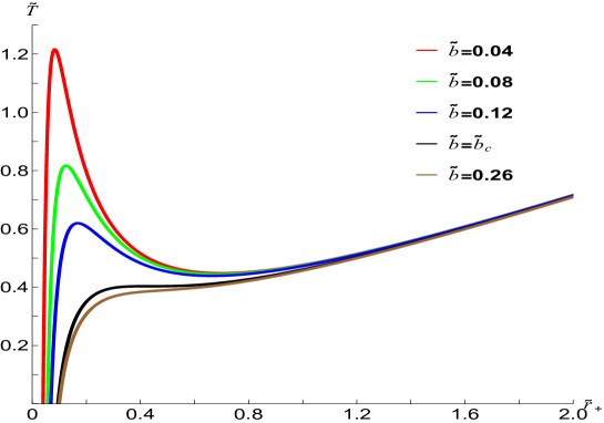
Figure 7: The temperature of the five-dimensional Kerr-AdS BH varies as a function of the horizon radius.

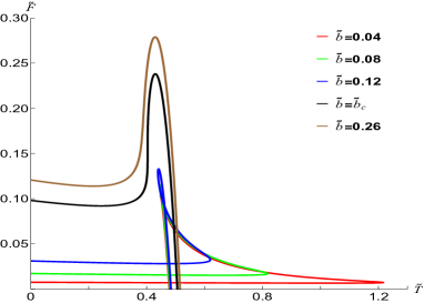
(a)

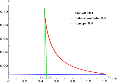
(b)

Figure 8: The free energy of the five-dimensional Kerr-AdS BH varies with the temperature. The scenario where $\tilde{b}=0.04$ is depicted in 8.

4.2 LEs and phase transitions

To investigate the relationship between the LEs and the phase transition of the five-dimensional Kerr-AdS BH, we initially compute the PTLEs and CTLEs in this section. Subsequently, we examine their relationships with the temperature.

When a particle moves in the equatorial plane of the BH, its Lagrangian is

$$\mathcal{L}=\frac{1}{2}\left(\tilde{g}_{tt}\dot{t}^{2}+\tilde{g}_{rr}\dot{r}^{2}+\tilde{g}_{\varphi\varphi}\dot{\varphi}^{2}+2\tilde{g}_{t\varphi}\dot{t}\dot{\varphi}\right).$$ (51)

Here $\tilde{g}_{\mu\nu}$ with $\mu,\nu=t,r,\varphi$ represent the components of the five-dimensional Kerr-AdS metric evaluated at $\theta=\frac{\pi}{2}$. Notably, the Lagrangian bears a resemblance to that presented in Eq. (21) for a particle in four-dimensional spacetime, with the primary difference lying in the expressions for the components,

$$\tilde{g}_{tt} = -\frac{1}{\tilde{\rho}^{2}}\left[\Delta_{r}-\tilde{\Delta}_{\theta}a^{2}-\frac{(1+r^{2}l^{-2})a^{2}b^{2}}{r^{2}}\right],\quad\tilde{g}_{rr}=\frac{\tilde{\rho}^{2}}{\Delta_{r}},$$

$$\tilde{g}_{\varphi\varphi} = \frac{1}{\tilde{\rho}^{2}\Xi_{a}^{2}}\left[-\Delta_{r}a^{2}+\tilde{\Delta}_{\theta}(r^{2}+a^{2})^{2}+\frac{(1+r^{2}l^{-2})(r^{2}+a^{2})^{2}b^{2}}{r^{2}}\right],$$

$$\tilde{g}_{t\varphi} = -\frac{1}{\tilde{\rho}^{2}\Xi_{a}}\left[\tilde{\Delta}_{\theta}a(r^{2}+a^{2})+\frac{(1+r^{2}l^{-2})(r^{2}+a^{2})ab^{2}}{r^{2}}-\Delta_{r}a\right],$$

$$\tilde{\rho}^{2} = r^{2}+b^{2},\quad\tilde{\Delta}_{\theta}=1-b^{2}l^{-2}.$$ (52)

Consequently, based on the calculations from the previous section, we get the radial equation of motion,

$$\dot{r}^{2}=\frac{\delta}{\tilde{g}_{rr}}-\frac{E^{2}\tilde{g}_{\varphi\varphi}+L^{2}\tilde{g}_{tt}+2EL\tilde{g}_{t\varphi}}{\tilde{g}_{rr}(\tilde{g}_{tt}\tilde{g}_{\varphi\varphi}-\tilde{g}_{t\varphi}^{2})},$$ (53)

where $\delta=0$ and $-1$ correspond to null and time-like geodesics, respectively.

4.2.1 Null geodesic’s case

From Eq. (53), the effective potential of a massless particle is derived,

$$V_{r}=\frac{(Ea-L\Xi_{a})^{2}\Delta_{r}l^{2}}{b^{2}r^{2}(r^{2}+l^{2})+l^{2}r^{4}\tilde{\Delta}_{\theta}}-\frac{\left[E(r^{2}+a^{2})-aL\Xi_{a})\right]^{2}}{r^{4}}.$$ (54)

The position of the unstable equilibrium orbit for particles is determined by solving the equations $V_{r}=V_{r}^{\prime}=0$. Utilizing Eqs. (10), (11) and (54), we obtain the values of the PTLE and CTLE at this orbit. Subsequently, we plot the curves illustrating their relationships with the temperature in Figure 9.

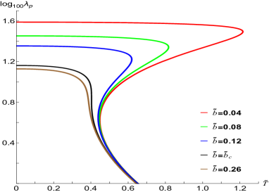
(a)

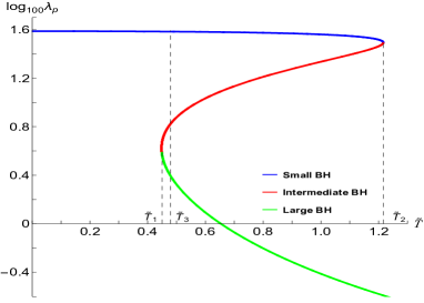
(b)

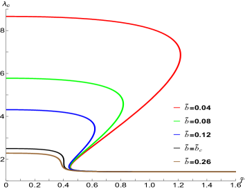
(c)

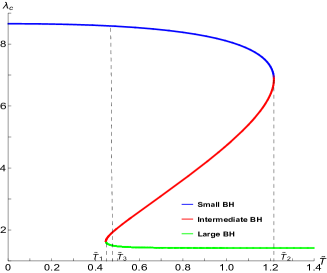
(d)

Figure 9: The variations of the PTLE and CTLE of chaos for the massless particle, as a function of the temperature of the five-dimensional Kerr-AdS BH. The specific scenarios with $\tilde{b}=0.04$ are plotted in 9 and 9, respectively.

In this figure, it is observed that when $\tilde{b}=0.26$, both the PTLE and CTLE exhibit a monotonic decrease as the temperature increases, suggesting the absence of any phase transition. Conversely, when $\tilde{b}<\tilde{b}_{c}$, both exponents take on multiple values, indicating the occurrence of phase transitions.

Figure 9 focuses specifically on the case where $\tilde{b}=0.04$. Within this context, the PTLE decreases monotonically with the temperature when $\tilde{T}<\tilde{T}_{1}$ and $\tilde{T}>\tilde{T}_{2}$. Notably, within the range $\tilde{T}_{1}<\tilde{T}<\tilde{T}_{2}$, each temperature corresponds to three distinct values of the exponent, representing the phases ofsmall, intermediate, and large BHs, respectively, which can interconvert within this temperature range. Notably, $\tilde{T}_{3}$ marks the temperature at which the first order phase transition occurs. It is noteworthy that $\tilde{T}_{1}$, $\tilde{T}_{2}$ and $\tilde{T}_{3}$ align precisely with their counterparts in Figure 8. Thus, the phase transition behavior of the five-dimensional Kerr-AdS BH can be characterized by the PTLE of chaos for the massless particle.

Figure 9 illustrates that at a lower temperature ($\tilde{T}<0.425$), the values of the CTLE corresponding to different rotational parameters are distinct. However, as the temperature increases, these values converge toward $1$. Figure 9 exhibits similarities with Figure 9: (1) When $\tilde{T}<\tilde{T}_{1}$ and $\tilde{T}>\tilde{T}_{2}$, both the PTLE and CTLE decrease monotonically with the temperature. (2) Within the range $\tilde{T}_{1}<\tilde{T}<\tilde{T}_{2}$, each temperature corresponds to three distinct values of the CTLE, which are associated with the phases of small, intermediate and large BHs. Consequently, the phase transition occurs within this temperature range. A notable difference arises when the temperature increases to a certain point: the CTLE approaches $1$, while the PTLE approaches $0$. Despite the disparity in the exponents’ values at the same temperature, they collectively describe the phase transition within the range $\tilde{T}_{1}<\tilde{T}<\tilde{T}_{2}$.

4.2.2 Timelike geodesic’s case

When the particle is massive, its motion obeys a time-like geodesic motion. Thus its effective potential is

$$V_{r}=-\frac{\Delta_{r}}{\tilde{\rho}^{2}}+\frac{(Ea-L\Xi_{a})^{2}\Delta_{r}l^{2}}{b^{2}r^{2}(r^{2}+l^{2})+l^{2}r^{4}\tilde{\Delta}_{\theta}}-\frac{\left[E(r^{2}+a^{2})-aL\Xi_{a})\right]^{2}}{r^{4}}.$$ (55)

We utilize Eqs. (10), (11) and (55) to obtain the PTLE and CTLE at an unstable equilibrium orbit. Subsequently, their relationships with the phase transition are explored.

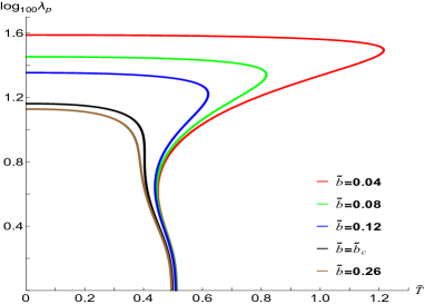
(a)

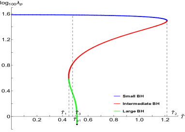
(b)

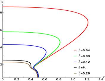
(c)

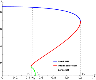
(d)

Figure 10: The variations of the PTLE and CTLE of chaos for the massive particle, as a function of the temperature of the five-dimensional Kerr-AdS BH. The specific scenarios with $\tilde{a}=\tilde{b}=0.04$ are plotted in 10 and 10, respectively.

Figure 10 displays the curves of the PTLE and CTLE of chaos for the massive particle as a function of the temperature. Notably, the values of $\tilde{a}$ and $\tilde{b}$ in this figure are identical to those in Figure 9. As expected, both the exponents decrease monotonically with increasing temperature when $\tilde{b}=0.26$ (as shown in Figures 10 and 10). When $\tilde{b}<\tilde{b}_{c}$, the PTLE and CTLE are multivalued functions, suggesting that the BH may have multiple phases at a given temperature.

Figure 10 illustrates the relationship between the PTLE and the temperature when $\tilde{b}=0.04$. This scenario resembles the behavior observed in the four-dimensional Kerr-AdS BH. Notably, there exists a terminal temperature $\tilde{T}_{p1}>0$ for the exponent. Within the range $\tilde{T}_{1}<\tilde{T}<\tilde{T}_{p1}$, phases of large, intermediate, and small BHs coexist, indicating the existence of a phase transition. However, for temperatures within $\tilde{T}_{p1}<\tilde{T}<\tilde{T}_{2}$, only intermediate and large BH phases persist. Consequently, the PTLE in this temperature range cannot reveal the phase transition between the large and small BHs.

A similar situation arises in Figure 10, where the terminal temperature for the exponent is denoted as $\tilde{T}_{p2}$. Specifically, at temperatures within $\tilde{T}_{1}<\tilde{T}<\tilde{T}_{p2}$, phases of large, intermediate and small BHs coexist. However, within the range $\tilde{T}_{p2}<\tilde{T}<\tilde{T}_{2}$, only intermediate and large BHs’ phases coexist. Thus it is only within the temperature range $\tilde{T}_{1}<\tilde{T}<\tilde{T}_{p2}$ that the CTLE can fully reveal the phase transition.

5 Conclusions and Discussions

In this paper, we explored the relationship between the PTLEs and CTLEs of chaos for the particles orbiting the four-dimensional and five-dimensional Kerr-AdS BHs and the BHs’ phase transitions. When examining the relationship between these exponents and the temperature, we observed that the exponents are single valued functions of the temperatures when the BHs’ rotational parameters exceed their critical values. Conversely, when the parameters fall below the critical values, the exponents transform into the multivalued functions of the temperature. By comparing these behaviors with the relationships between free energy and the temperature, we found that both types of exponents can describe the phase transitions. The critical exponents associated with the CTLEs and PTLEs were found to be 1/2.

For the massless particles, within a specific temperature range, each temperature corresponds to three distinct values of both the PTLEs and CTLEs, which correspond to the phases of the small, intermediate and large BHs, respectively. Consequently, the phase transitions can occur within this temperature range, which aligns perfectly with the range where the free energies change with the temperature. Therefore, these two types of exponents are capable of describing the phase transitions. For the massive particles, the PTLEs and the CTLEs correspond to the different terminal temperatures, respectively. The emergence of these terminal temperatures signifies the disappearance of the unstable equilibrium orbits at these specific temperatures. At the terminal temperatures, the PTLEs have the values greater than $0$, while the CTLEs equal $0$.

In the case of the four-dimensional Kerr-AdS BH, the phases of large, intermediate and small BHs can coexist only within the temperature ranges $\bar{T}_{1}<\bar{T}<\bar{T}_{p1}$ and $\bar{T}_{1}<\bar{T}<\bar{T}_{p2}$. However, within the ranges $\bar{T}_{p1}<\bar{T}<\bar{T}_{2}$ and $\bar{T}_{p2}<\bar{T}<\bar{T}_{2}$, the coexistence is limited to the phases of intermediate and large BHs. Consequently, within these specified temperature ranges, the exponents are inadequate for describing the phase transitions. A similar scenario arises in the five-dimensional Kerr-AdS BH.

In conclusion, both the PTLEs and CTLEs are adept at describing the phase transitions of the four-dimensional and five-dimensional Kerr-AdS BHs. Nevertheless, the LEs of chaos for the massless particles offer a more effective depiction of the phase transitions compared to those of the massive particles.

- (1)
- (2) D. Pugliese, H. Quevedo, and R. Ruffini, Circular motion of neutral test particles in Reissner-Nordstrom spacetime, Phys. Rev. D 83 (2011) 024021. arXiv:1012.5411 [astro-ph.HE].
- (3) C.Y. Liu, D.S. Lee and C.Y. Lin, Geodesic motion of neutral particles around a Kerr–Newman black hole, Class. Quant. Grav. 34 (2017) 235008. arXiv:1706.05466 [gr-qc].
- (4) Y.P. Zhang, S.W. Wei, P. Amaro-Seoane, J. Yang and Y.X. Liu, Motion deviation of test body induced by spin and cosmological constant in extreme mass ratio inspiral binary system, Eur. Phys. J. C 79 (2019) 856.
- (5) M. Zhang and W.B. Liu, Innermost stable circular orbits of charged spinning test particles, Phys. Lett. B 789 (2019) 393.
- (6) D.N. Page and K.S. Thorne, Disk-accretion onto a black hole. Time-averaged structure of accretion disk, Astrophys. J. 191 (1974) 499.
- (7) The Event Horizon Telescope Collaboration et al, First M87 event horizon telescope results. I. The shadow of the supermassive black hole, Astrophys. J. Lett. 875 (2019) L1.
- (8) The Event Horizon Telescope Collaboration et al, First M87 event horizon telescope results. IV. Imaging the central supermassive black hole, Astrophys. J. Lett. 875 (2019) L4.
- (9) The Event Horizon Telescope Collaboration et al, First M87 event horizon telescope results. V. Physical origin of the asymmetric ring, Astrophys. J. Lett. 875 (2019) L5.
- (10) The Event Horizon Telescope Collaboration et al, First M87 event horizon telescope results. VI. The shadow and mass of the central black hole, Astrophys. J. Lett. 875 (2019) L6.
- (11) R.A. Konoplya, A. Zhidenko, Quasinormal modes of black holes: from astrophysics to string theory, Rev. Mod. Phys. 83 (2011) 793.
- (12) B.P. Abbott et al., (LIGO Scientific Collaboration and Virgo Collaboration), Observation of gravitational waves from a binary black hole merger, Phys. Rev. Lett. 116 (2016) 061102.
- (13) B.P. Abbott et al., (LIGO Scientific Collaboration and Virgo Collaboration), Tests of general relativity with GW150914, Phys. Rev. Lett. 116 (2016) 221101.
- (14) B.P. Abbott et al., (LIGO Scientific Collaboration and Virgo Collaboration), GW151226: Observation of gravitational waves from a 22-solar-mass binary black hole coalescence, Phys. Rev. Lett. 116 (2016) 241103.
- (15) W.L. Ames and K.S. Thorne, The optical appearance of a star that is collapsing through its gravitational radius, Astrophys. J. 151 (1968) 659.
- (16) K. Hashimoto1 and N. Tanahashi, Universality in chaos of particle motion near black hole horizon, Phys. Rev. D 95 (2017) 024007.
- (17) S. Suzuki and K.i. Maeda, Signature of chaos in gravitational waves from a spinning particle, Phys. Rev. D 61 (2000) 024005.
- (18) S. Suzuki and K.i. Maeda, Gravitational waves from chaotic dynamical system, Phys. Rev. D 70 (2004) 064036 .
- (19) S. Suzuki and K.i. Maeda, Gravitational wave signals from chaotic system: a point mass with a disk, Phys. Rev. D 76 (2007) 024018.
- (20) V.D. Falco and W. Borrelli, Detection of chaos in the general relativistic Poynting-Robertson effect: Kerr equatorial plane, Phys. Rev. D 103 (2021) 064014.
- (21) V.D. Falco and W. Borrelli, Timescales of the chaos onset in the general relativistic Poynting-Robertson effect, Phys. Rev. D 103 (2021) 124012.
- (22) S.W. Hawking and D.N. Page, Thermodynamics of black holes in Anti-de Sitter space, Commun. Math. Phys. 87 (1983) 577.
- (23) D. Kastor, S. Ray and J. Traschen, Enthalpy and the mechanics of AdS black holes, Class. Quantum Gravity 26 (2009) 195011.
- (24) D. Kastor, S. Ray and J. Traschen, Smarr formula and an extended first law for lovelock gravity, Class. Quantum Gravityy 27 (2010) 235014.
- (25) D. Kubiznak and R.B. Mann, P-V criticality of charged AdS black holes, JHEP 1207 (2012) 033.
- (26) D. Kubiznak and R.B. Mann, Black hole chemistry, Can. J. Phys. 93 (2015) 999.
- (27) R.G. Cai, L.M. Cao, L. Li, and R.Q. Yang, P-V criticality in the extended phase space of Gauss-Bonnet black holes in AdS space, JHEP 09 (2013) 005.
- (28) R.G. Cai, Oscillatory behaviors near a black hole triple point Sci. China Phys. Mech. Astron. 64 (2021) 290432.
- (29) S.W. Wei and Y.X. Liu, Triple points and phase diagrams in the extended phase space of charged Gauss-Bonnet black holes in AdS space, Phys. Rev. D 90 (2014) 044057.
- (30) S.W. Wei, Y.X. Liu, Insight into the microscopic structure of an AdS black hole from a thermodynamical phase transition, Phys. Rev. Lett. 115 (2015) 111302.
- (31) S.W. Wei, Y.X. Liu, R.B. Mann, Repulsive interactions and universal properties of charged anti-de Sitter black hole microstructures, Phys. Rev. Lett. 123 (2019) 071103.
- (32) S. Gunasekaran, R.B. Mann and D. Kubiznak, Extended phase space thermodynamics for charged and rotating black holes and Born-Infeld vacuum polarization, JHEP 1211 (2012) 110.
- (33) J.F. Xu, L.M. Cao and Y.P. Hu, P-V criticality in the extended phase space of black holes in massive gravity, Phys. Rev. D 91 (2015) 124033.
- (34) D. Kubiznak, R.B. Mann and M. Teo, Black hole chemistry: thermodynamics with Lambda, Class. Quant. Grav. 34 (2017) 063001.
- (35) N. Altamirano, D. Kubiznak, R.B. Mann and Z. Sherkatghanad, Kerr-AdS analogue of triple point and solid/liquid/gas phase transition, Class. Quant. Grav. 31 (2014) 042001.
- (36) M. Zhang, S.Z. Han, J. Jiang and W.B. Liu, Circular orbit of a test particle and phase transition of a black hole, Phys. Rev. D 99 (2019) 065016.
- (37) N. Altamirano, D. Kubiznak and R.B. Mann, Reentrant phase transitions in rotating anti-de Sitter black holes, Phys. Rev. D 88 (2013) 101502(R).
- (38) J.F. Xu, L.M. Cao and Y.P. Hu, P-V criticality in the extended phase space of black holes in massive gravity, Phys. Rev. D 91 (2015) 124033.
- (39) D.C. Zou, Y.Q. Liu and R.H. Yue, Behavior of quasinormal modes and Van der Waals-like phase transition of charged AdS black holes in massive gravity, Eur. Phys. J. C 77 (2017) 365.
- (40) D.C. Zou, R. Yue and M. Zhang, Reentrant phase transitions of higher-dimensional AdS black holes in dRGT massive gravity, Eur. Phys. J. C 77 (2017) 256..
- (41) D.V. Singh and S. Siwach, Thermodynamics and P-v criticality of Bardeen-AdS black hole in 4-D Einstein-Gauss-Bonnet gravity, Phys. Lett. B 808 (2020) 135658.
- (42) R.A. Hennigar, R.B. Mann and E. Tjoa, Superfluid Black Holes, Phys. Rev. Lett. 118 (2017) 021301.
- (43) S.W. Wei and Y.X. Liu, Triple points and phase diagrams in the extended phase space of charged Gauss-Bonnet black holes in AdS space, Phys. Rev. D 90(2014) 044057 .
- (44) A.M. Frassino, D. Kubiznak, R.B. Mann and F. Simovic, Multiple reentrant phase transitions and triple points in Lovelock thermodynamics, JHEP 1409 (2014) 080.
- (45) G.Z. Guo, P. Wang, H.W. Wu and H.T. Yang, Thermodynamics and phase structure of an Einstein-Maxwell-scalar model in extended phase space, Phys. Rev. D 105 (2022) 064069.
- (46) S.Q. Lan, J.X. Mo, G.Q. Li and X.B. Xu, Effects of dark energy on dynamic phase transition of charged AdS black holes, Phys. Rev. D 104 (2021) 104032.
- (47) S.H. Hendi and K. Jafarzade, Critical behavior of charged AdS black holes surrounded by quintessence via an alternative phase space, Phys. Rev. D 103 (2021) 104011.
- (48) Y.Z. Du, H.F. Li and L.C. Zhang, Continuous phase transition of higher-dimensional de-Sitter spacetime with non-linear source, Eur. Phys. J. C 82 (2022) 370.
- (49) X.B. Guo, Y. Lu, B.R. Mu and P. Wang, Probing phase structure of black holes with Lyapunov exponents, JHEP 08 (2022) 153.
- (50) S.J. Yang, J. Tao, B.R. Mu and A.Y. He, Lyapunov exponents and phase transitions of Born-Infeld AdS black holes, JCAP 07 (2023) 045.
- (51) X. Lyu, J. Tao and P. Wang, Probing the thermodynamics of charged Gauss Bonnet AdS black holes with the Lyapunov exponent, Eur. Phys. J. C 84 (2023) 974.
- (52) A.N. Kumara, S. Punacha and M.S. Ali, Lyapunov exponents and phase structure of Lifshitz and Hyperscaling violating black holes, JCAP 84 (2024) 061.
- (53) Y.Z. Du, H.F. Li, Y.B. Ma and Q. Gu, Phase structure of the de Sitter spacetime with KR field based on the Lyapunov exponent, e-Print: 2403.20083 [hep-th].
- (54) B. Shukla, P.P. Das, D. Dudal and S. Mahapatra, Interplay between the Lyapunov exponents and phase transitions of charged AdS black holes, Phys. Rev. D 110 (2024) 024068.
- (55) N.J. Gogoi, S. Acharjee and P. Phukon, Lyapunov exponents and phase transition of Hayward AdS black hole, Eur. Phys. J. C 84 (2024) 1144.
- (56) V. Cardoso, A.S. Miranda, E. Berti, H. Witek and V.T. Zanchin, Geodesic stability, Lyapunov exponents and quasinormal modes, Phys. Rev. D 79 (2009) 064016.
- (57) P.P. Pradhan, Lyapunov exponent and charged Myers Perry spacetimes, Eur. Phys. J. C 73 (2013) 2477.
- (58) P.P. Pradhan, Stability analysis and quasinormal modes of Reissner-Nordstrom space-time via Lyapunov exponent, Pramana 87 (2016) 5.
- (59) P.P. Pradhan, Circular geodesics in tidal charged black hole, Int. J. Geom. Meth. Mod. Phys. 15 (2017) 1850011.
- (60) Y.Q. Lei, X.H. Ge and C. Ran, Chaos of particle motion near a black hole with quasitopological electromagnetism, Phys. Rev. D 104 (2021) 046020.
- (61) Y.Q. Lei and X.H. Ge, Circular motion of charged particles near charged black hole, Phys. Rev. D 105 (2022) 084011.
- (62) C.H. Gao, D.Y. Chen, C.Y. Yu and P. Wang, Chaos bound and its violation in charged Kiselev black hole, Phys. Lett. B 105 833 (2022) 137343.
- (63) N. Altamirano, D. Kubiznak, R.B. Mann and Z. Sherkatghanad, Kerr-AdS analogue of triple point and solid/liquid/gas phase transition, Class. Quant. Grav. 31 (2014) 042001.
- (64) N. Altamirano, D. Kubiznak, R.B. Mann and Z. Sherkatghanad, Thermodynamics of rotating black holes and black rings: phase transitions and thermodynamic volume, Galaxies 2 (2014) 89.
- (65) S.J Yang, R. Zhou, S.W. Wei and Y.X. Liu, Kinetics of a phase transition for a Kerr-AdS black hole on the free-energy landscape, Phys. Rev. D 105 (2022) 084030.
- (66) P. Cheng, J.D Pan, H.C. Xu, S.J. Yang, Thermodynamics of the Kerr-AdS black hole from an ensemble-averaged theory, arXiv:2410.23006 [hep-th]
- (67) J. Maldacena, S.H. Shenker and D. Stanford, A bound on chaos, JHEP 08 (2016) 106.
- (68) Q.Q. Zhao, Y.Z. Li and H. Lü, Static equilibria of charged particles around charged black holes: Chaos bound and its violations, Phys. Rev. D 98 (2018) 124001.
- (69) N. Kan and B. Gwak, Bound of the Lyapunov exponent in Kerr-Newman black holes via a charged particle, Phys. Rev. D 105 026006 (2022).
- (70) B. Gwak, N. Kan, B.H. Lee and H. Lee, Violation of bound on chaos for charged probe in Kerr-Newman-AdS black hole, JHEP 09 (2022) 026.
- (71) R. Banerjee, D. Roychowdhury, Critical phenomena in Born-Infeld AdS black holes, Phys. Rev. D 85 (2012) 044040.
- (72) R. Banerjee and D. Roychowdhury, Critical behavior of Born Infeld AdS black holes in higher dimensions, Phys. Rev. D 85 (2012) 104043.
- (73) S.W. Hawking, C.J. Hunter and M.M. Taylor-Robinson, Rotation and the AdS/CFT correspondence, Phys. Rev. D 59 (1999) 064005.