Artificial Intelligence Clones

Abstract.

Large language models, trained on personal data, may soon be able to mimic individual personalities. This would potentially transform search across human candidates, including for marriage and jobs—indeed, several dating platforms have already begun experimenting with training “AI clones” to represent users. This paper presents a theoretical framework to study the tradeoff between the substantially expanded search capacity of AI clones and their imperfect representation of humans. Individuals are modeled as points in $k$-dimensional Euclidean space, and their AI clones are modeled as noisy approximations. I compare two search regimes: an “in-person regime”—where each person randomly meets some number of individuals and matches to the most compatible among them—against an “AI representation regime”—in which individuals match to the person whose AI clone is most compatible with their AI clone. I show that a finite number of in-person encounters exceeds the expected payoff from search over infinite AI clones. Moreover, when the dimensionality of personality is large, simply meeting two people in person produces a higher expected match quality than entrusting the process to an AI platform, regardless of the size of its candidate pool.

1. Introduction

Recent advances in large language models have brought us closer to a world in which artificial intelligence—trained on vast collections of written and spoken communications—can convincingly mimic individual personalities. This development has the potential to transform search over human candidates in various contexts. Several dating platforms have already begun developing “AI clones” of individual users to simulate dialogues between potential matches (Metz, 2024),^, and the conceivable applications of AI clones extend to many other domains as well. For example, organizations could employ AI clones of recruiters and applicants to simulate interviews with a large pool of candidates, or a placement agency—such as one that matches families to caregivers—might rely on AI clones to assess whether a prospective caregiver fits with a family. These examples highlight the potential for artificial intelligence to reshape how people identify, evaluate, and ultimately choose one another across a wide array of personal and professional settings.

Relative to in-person interactions, the primary appeal of AI clones is their capacity to search across a large pool of potential matches. However, unlike actual clones that replicate an individual precisely, AI clones must approximate their subject’s personality from limited training data. This challenge is compounded by the complexity of the target: a complete human personality.

This paper examines whether the search advantage offered by AI representations outweighs the inaccuracies they introduce. To address this question, I develop a model in which individuals are represented as vectors in a finite-dimensional Euclidean space, where each element of this vector is an attribute of personality (broadly construed). Individuals prefer to be matched to others close to them in this space, i.e., to another with similar personality attributes. I consider two scenarios from the perspective of an individual referred to as “Subject”: in the first scenario, the in-person regime, Subject meets $m$ randomly selected individuals and matches to the closest of these individuals; in the second scenario, the AI representation regime, Subject’s match is the individual whose AI clone is most similar to Subject’s own AI clone. I show that there exists a finite $m$ such that meeting $m$ individuals in person yields a better expected match than the AI platform, even when the platform searches over infinitely many candidates. Moreover, when the dimensionality of personality is large, this $m$ equals two. In other words, as personality complexity increases, simply meeting two people in person produces a higher expected match quality than entrusting the process to an AI platform, regardless of the size of its candidate pool.

In more detail: I model individuals as vectors in $k$-dimensional Euclidean space, where Subject is placed at the zero vector and all other individuals are drawn uniformly from the unit ball. In the in-person regime, Subject randomly meets $m$ individuals and observes their attributes. Subject matches to the closest of these $m$ individuals, and receives a payoff equal to the negative of the Euclidean distance between them. In the AI representation regime, all individuals are represented by AI clones, which are imperfect approximations of the individuals’ personalities. Specifically, an individual’s AI clone is the individual’s true personality vector perturbed by a multivariate Gaussian noise term. The AI clones interact, and the match quality between these clones is determined. Subject is matched to the individual whose AI clone is most compatible to Subject’s AI clone, but Subject’s payoff is the negative of the true distance between them.

This model is inspired by AI clones, but can be interpreted as more generally describing situations in which the search objective and the candidates are too complex to be completely specified. In these settings there are inherent limits to how well search can be automated, since each candidate must be evaluated with respect to the system’s imperfect understanding of that candidate and the objective. In contrast, an actor who has internalized a rich, nuanced understanding of what constitutes a “good” match—be it a romantic partner, a new hire, or any other complex target—can more accurately evaluate each candidate. Since a human actor can only evaluate a limited number of candidates in this way, the key comparison is between the capacity constraints of human evaluation and the approximation errors of automated search.

My results pertain to a quantity I call the AI-equivalent sample size, which measures the value of the AI platform. The AI-equivalent sample size is the smallest $m$ such that if Subject is permitted $m$ draws in the in-person regime, then no search advantage given to the AI representation regime can compensate for the error introduced by the AI clones. That is, Subject would rather meet $m$ individuals in person than search over an infinite number of individuals on the AI platform.

My first main result, Proposition 4.1, says that the AI-equivalent sample size is always finite. In other words, for any level of AI approximation error, there exists a finite number of in-person encounters sufficient to outperform any search advantage offered by the AI platform. Intuitively, as the number of individuals on the AI platform grows large, the individual identified as the best match will have an AI clone that (nearly) perfectly matches Subject’s AI clone. But because these clones imperfectly represent their human counterparts, there is always some expected mismatch between the underlying humans—even when the AI clones are perfectly compatible. In contrast, in the in-person regime, the best of $m$ draws will eventually approach a perfect match, and thus sufficiently many such draws must outperform the AI platform.

My second main result, Theorem 4.1, shows that when the number of dimensions of personality is large, then the AI-equivalent sample size is simply two. That is, the in-person regime yields a higher expected payoff so long as Subject can search over at least two people.

To understand this result, we need to consider the role of the dimensionality of the personality space. High-dimensional spaces exhibit several interesting properties: Random points in the unit ball tend to be far from one another, and the distances between them concentrate around their expected values. In the context of my model, this means that each individual becomes increasingly unique in the personality space. This scarcity of nearby individuals creates two opposing effects. On the one hand, searching through more candidates has greater value, since doing so increases the chance of finding someone compatible—an advantage that favors the AI representation regime. At the same time, the increase in complexity of the learning problem means that the errors of the AI representation regime are more consequential. Theorem 4.1 says that this latter effect dominates.

Formally, I show that as the number of dimensions grows large, Subject’s expected payoff in the AI representation regime converges to the benchmark payoff from being matched to a single randomly drawn individual. Loosely speaking, this is because the problem of estimation in high dimensions becomes so difficult that the match identified on the AI platform is driven by the noise in the estimation, rather than by actual compatibility. At the same time, the single random draw benchmark is also the limiting expected payoff from being matched to the better of two draws in the in-person regime. The key step towards proving the result is thus to show that the benefit provided by the AI platform erodes more rapidly than the benefit of having a second in-person draw.

In the final part of the paper, I explore an extension in which the AI platform has access to different quantities of data for different individuals, reflecting heterogeneity in data availability due to factors like privacy preferences or digital presence. Individuals are categorized into two groups, a “data-rich” and “data-poor” group, which are differentiated by the quality of AI estimation. Despite the groups being otherwise identical in characteristics, I show that Subject is matched to a data-rich individual with probability exceeding one-half, and moreover that this probability converges to 1 as either the dimensionality of analysis increases or the disparity in estimation errors between groups widens. These results suggest a new form of social stratification, where individuals’ outcomes depend not just on their intrinsic characteristics but also on how well they are understood by AI systems.

The remainder of the paper is organized as follows. Section 2 describes the model. Section 3 considers the simple case of a single dimension. Section 4 presents the main results. Section 5 presents the extension to heterogenous individuals, and Section 6 concludes.

1.1. Related Literature

This paper contributes to a growing literature on the social implications of artificial intelligence (AI), in particular to research comparing human and AI evaluation. AI predictions have been shown to outperform human experts across various prediction problems (Rajpurkar et al., 2017; Jung et al., 2017; Agarwal et al., 2023; Kleinberg et al., 2017; Angelova et al., 2022); Iakovlev and Liang (2024) provide a theoretical rationale for why this might be so. These papers all consider settings—such as medical diagnosis—where humans possess limited intuitive knowledge about the underlying decision problem. By contrast, the present paper is motivated by settings where human actors possess a naturally rich understanding of a complex, subjective objective, which is difficult to define formally. This is a novel consideration relative to the literature, and the paper arrives at a very different conclusion regarding algorithmic versus human evaluation.

This work also contributes to the rich literature on search, which has explored classic questions including how long to search for (Stigler, 1961; McCall, 1970; Weitzman, 1979), what speed to search at (Urgun and Yariv, 2024), and where to search (Callander, 2011; Malladi, 2023). The present paper focuses on a new question regarding the role of the complexity of the search space, as measured by the number of attributes (Klabjan et al., 2014). I show that dimensionality fundamentally alters optimal search behavior when search is conducted with error. This result contrasts with, for example, Bardhi (2023) and Malladi (2023), who show that their characterizations of optimal search extend but are not qualitatively changed in multiple dimensions.

Key to Theorem 4.1 is a comparison of asymptotics as the dimensionality of the search space grows large. Rates of convergence results have a long history in economic theory, but typically involve limits in the quantity of information (Vives, 1992; Moscarini and Smith, 2002; Liang and Mu, 2019; Frick et al., 2024) or the size of a population (Harel et al., 2021; Dasaratha et al., 2023). Iakovlev and Liang (2024) consider a similar asymptotic to the present paper (i.e., with respect to an increasing number of attributes) but characterize limiting beliefs rather than the limiting value of search.

Finally, while this paper adopts the narrative of a dating platform, it diverges considerably both from the classic matching frameworks (Gale and Shapley, 1962; Roth and Sotomayor, 1992), which examine how centralized mechanisms can achieve stable or efficient outcomes for populations, and from the search and matching literature (Shimer and Smith, 2000; Chade et al., 2017), which analyzes macroecononmic outcomes and equilibrium behavior in decentralized markets with many searchers. This paper instead focuses on the decision problem of a single agent navigating a high-dimensional search space.

2. Model

Each individual $i$ is described by $k$ real-valued personality attributes. I consider the perspective of a specific individual, subsequently ‘Subject,’ whose attributes are fixed at the zero vector $x_{0}$. Every other individual $X_{i}\in\mathbb{R}^{k}$, $i\geq 1$, is drawn uniformly at random from the $k$-dimensional unit ball $B_{k}\equiv\{x\in\mathbb{R}^{k}:\|x\|\leq 1\}$. Subject receives utility $-\|X_{i}-x_{0}\|=-\|X_{i}\|$ from being matched to individual $i$, i.e., the negative of the Euclidean distance between them. I will use the phrases “most similar individual,” “closest individual,” and “most compatible individual” interchangeably. (See Section 4.1 for discussion of other notions of match quality.)

There are two regimes. In the first, which I call the in-person regime, Subject randomly meets $m$ individuals and matches to the closest individual. The expected distance to this individual in $k$ dimensions is

$$d^{\text{IP}}_{k}(m)\equiv\mathbb{E}\left[\min_{1\leq i\leq m}\|X_{i}\|\right]$$

and Subject’s expected payoff is $-d^{\text{IP}}_{k}(m)$.

In the second regime, which I call the AI representation regime, individuals do not interact in person; instead, they elect to have an AI clone represent them, and these clones interact with one another. Each clone is a random imperfect mimic of each individual, and match quality is estimated based on compatibility of the realized AI clones. Formally, in an interaction between Subject and individual $i$, Subject is represented by

$$Y_{0i}=x_{0}+\varepsilon_{0i}$$

and individual $i$ is represented by

$$Y_{i0}=X_{i}+\varepsilon_{i0}$$

where $\varepsilon_{0i},\varepsilon_{i0}\sim\mathcal{N}(0,\sigma^{2}I_{k})$ are multivariate Gaussian noise terms that are independent of each other and across $i$. The notation $I_{k}$ denotes the identity matrix in $k$ dimensions, and I assume throughout that $\sigma^{2}>0$. See Figure 1 for a depiction of the model in three dimensions, i.e., $k=3$.

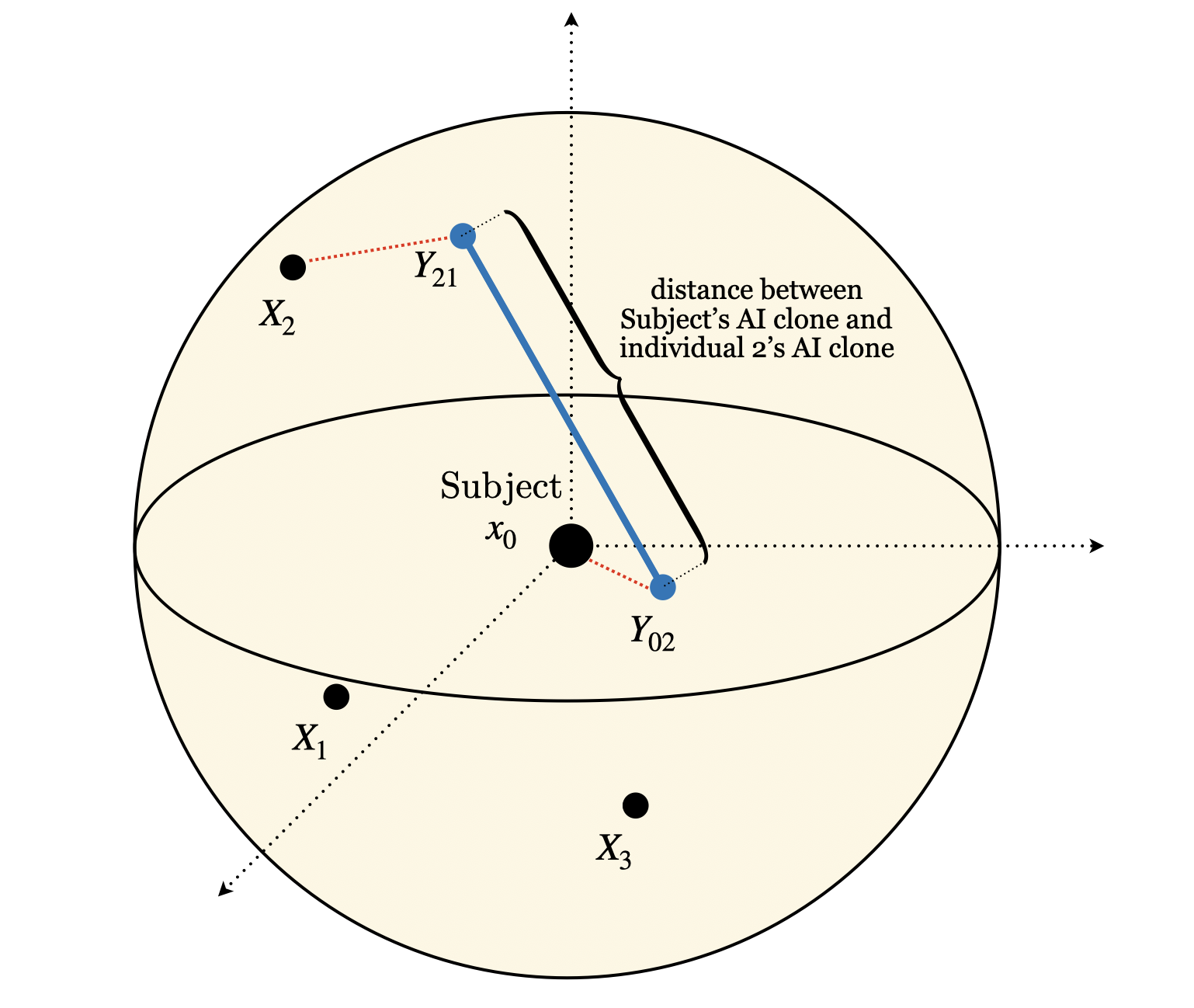
Figure 1. Depiction of an interaction between Subject’s AI clone and individual 2’s AI clone in $k=3$ dimensions.

The AI platform searches over $n$ possible matches for Subject. Among these, the individual with the most compatible AI clone is

$$i^{*}_{n}=\operatorname*{arg\,min}_{1\leq i\leq n}\|Y_{0i}-Y_{i0}\|.$$

Subject’s expected actual distance to this individual is

$$d^{\text{AI}}_{k}(n)\equiv\mathbb{E}\left[\|X_{i^{*}_{n}}\|\right].$$

I again make the number of dimensions $k$ explicit, as this is a parameter that we will vary.

While the dating platform serves as the main narrative throughout the paper, this model can also be used to consider other uses of AI clones, such as the following.

Example (Job Hiring).

A firm seeks a suitable candidate from a large pool of applicants. In the in-person regime, the hiring manager interviews some $m$ candidates in person. In the AI representation regime, an AI clone of the hiring manager conducts interviews with the AI clones representing some $n$ candidates.

Example (Family-to-Caregiver Matching).

A family seeks to hire a caregiver. In the in-person regime, the family meets with several candidates. In the AI representation regime, AI clones of the family members interact with AI clones of the potential caregivers.

Example (Collaboration).

An engineer seeks a collaborator to manage the business side of a startup. In the in-person regime, the engineer interacts with potential collaborators at networking events. In the AI representation regime, AI clones of the engineer and potential collaborators interact and are assessed on joint collaborative potential.

Beyond AI clones, we can think of the model as more generally describing situations where both the objects of search as well as the desired objective are complex.

Example (Purchasing a Home).

A family seeks to purchase a home. In the in-person regime, the family visits a small number of houses in person. In the AI representation regime, the family’s preferences are communicated as best possible to an AI system, which then (imperfectly) evaluates many homes with respect to this objective.

The key point is that there are tasks that are simple for humans but challenging for machines. A human knows intuitively that they prefer one person’s company over another, and that they feel more at home in one house than another, even when the underlying reasons are complex and challenging to specify for an algorithm. Moreover, the sheer number of subtle factors—such as whether someone’s sense of humor is dry or dark—implies that even if a machine fully understood the objective function, it would still need a profound understanding of each candidate to make an accurate assessment. Ultimately, there is a tradeoff between a fast automated approach that produces less accurate evaluations and a more resource-intensive method that relies on knowledgeable human judgment to yield precise assessments.

My results pertain to a quantity I call the sample size equivalent of the idealized AI representation regime with $n=\infty$.

Definition 2.1.

Fix any dimension $k$. The AI-equivalent sample size $m^{*}_{k}$ is the smallest $m\in\mathbb{Z}_{+}$ satisfying

$$\mathbb{E}\left[d^{\text{IP}}_{k}(m)\right]<\mathbb{E}\left[d^{\text{AI}}_{k}(n)\right]\quad\forall n\in\mathbb{Z}_{+}.$$

If the inequality above is not satisfied for any finite $m$, then $m^{*}_{k}=\infty$.

The AI-equivalent sample size $m^{*}_{k}$ provides a measure of the value of the AI platform. If $m^{*}_{k}$ is infinite, then every in-person search can be beat by an AI platform with a large enough candidate pool. If $m^{*}_{k}$ is instead finite, then the advantage of the AI platform is fundamentally capped, and a sufficiently thorough in-person search will outperform it. In this case, a small $m^{*}_{k}$ suggests that even a small number of in-person encounters can outperform the AI platform’s infinite search capacity, while a larger (but still finite) $m^{*}_{k}$ indicates that the AI platform retains a noticeable advantage before in-person search can catch up. In this way, $m^{*}_{k}$ serves as a practical yardstick for determining when and how human efforts can prevail over algorithmic methods.

3. Warm-Up: One Dimension

To build intuition, let us first consider the one-dimensional case. Subject is located at zero, and all other individuals in the population are drawn uniformly from $[-1,1]$. For any distance $r\in[0,1]$,

$$P\left(\min_{1\leq i\leq m}|X_{i}|>r\right)=P(|X_{1}|>r)^{m}=(1-r)^{m}$$

since $X_{i}$ are i.i.d. So Subject’s expected distance to the best match among $m$ draws in the in-person regime is

$$d^{\text{IP}}_{1}(m)=\mathbb{E}\left[\min_{1\leq i\leq m}|X_{i}|\right]=\int_{0}^{1}P\left(\min_{1\leq i\leq m}|X_{i}|>r\right)dr=\int_{0}^{1}(1-r)^{m}dr=\frac{1}{m+1}.$$

Now consider the AI representation regime. In the proof of Proposition 4.1, I show that Subject’s expected payoff given $n$ samples can be lower bounded by Subject’s expected payoff in an “infinite $n$” setting in which $|Y_{i0}-Y_{0i}|=0$ is achieved for some index $i$, i.e., there is some AI clone that perfectly matches Subject’s AI clone. Conditional on the event $\{|Y_{i0}-Y_{0i}|=0\}$, the random variable $X_{i}$ (the actual location of individual $i$) is independent of all other $X_{j}$ and $Y_{j0}$ (the actual locations and clone realizations of the other individuals). Thus we can write Subject’s expected payoff as

$$d^{\text{AI}}_{k}(\infty)=\mathbb{E}\left(|X_{i}|:|Y_{i0}-Y_{0i}|=0\right).$$

To characterize this conditional expectation, observe that the distance between Subject’s AI clone, $Y_{0i}$, and the AI clone of individual $i$, $Y_{i0}$, is

$$|Y_{i0}-Y_{0i}|=|X_{i}+\varepsilon_{i0}-\varepsilon_{0i}|=|X_{i}+Z_{i}|$$

where $Z_{i}\equiv\varepsilon_{i0}-\varepsilon_{0i}\sim\mathcal{N}(0,2\sigma^{2})$. So $|Y_{i0}-Y_{0i}|=0$ implies $Z_{i}=-X_{i}$. That is, if the $i$-th AI clone perfectly matches Subject’s AI clone, it must be that the noise term $Z_{i}$ exactly undoes the true distance between Subject and individual $i$.

By independence of $X_{i}$ and $Z_{i}$, and symmetry of $Z_{i}$, we have

$$P(|X_{i}|>r\mid Z_{i}=-X_{i}) =\frac{\int_{-1}^{-r}f_{X_{i}}(x)f_{Z_{i}}(x)dx+\int_{r}^{1}f_{X_{i}}(x)f_{Z_{i}}(x)dx}{\int_{-1}^{1}f_{X_{i}}(x)f_{Z_{i}}(x)dx}$$

$$=\frac{2\int_{-1}^{-r}f_{Z_{i}}(x)dx}{\int_{-1}^{1}f_{Z_{i}}(x)dx}\quad\quad\mbox{since $f_{X_{i}}(x)=\frac{1}{2}\mathbbm{1}(x\in[-1,1])$}$$

$$=2\frac{\Phi\left(-\frac{r}{\sqrt{2}\sigma}\right)-\Phi\left(-\frac{1}{\sqrt{2}\sigma}\right)}{\Phi\left(\frac{1}{\sqrt{2}\sigma}\right)-\Phi\left(-\frac{1}{\sqrt{2}\sigma}\right)}$$

where $\Phi$ denotes the CDF of the standard normal distribution. Thus

$$d^{\text{AI}}_{k}(\infty)=\mathbb{E}[|X_{i}|:Z_{i}=-X_{i}] =\int_{0}^{1}P(|X_{i}|>r\mid Z_{i}=-X_{i})dr$$

$$=2\int_{0}^{1}\frac{\Phi\left(-\frac{r}{\sqrt{2}\sigma}\right)-\Phi\left(-\frac{1}{\sqrt{2}\sigma}\right)}{\Phi\left(\frac{1}{\sqrt{2}\sigma}\right)-\Phi\left(-\frac{1}{\sqrt{2}\sigma}\right)}dr:=\varphi(\sigma)$$

This expression is strictly positive while $d^{\text{IP}}_{1}(m)=\frac{1}{m+1}$ converges to zero as $m$ grows large. Setting

$$m^{*}_{1}=\left\lceil\frac{1}{\varphi(\sigma)}-1\right\rceil+1<\infty$$

we have $d^{\text{IP}}_{1}(m_{1}^{*})<d^{\text{AI}}_{1}(\infty)$, i.e., Subject prefers the in-person regime (in one dimension) with a sample size of $m^{*}_{1}$ individuals over the AI representation regime (in one dimension) with an infinite number of individuals. This $m^{*}_{1}$ need not be very large; for example, if $\sigma=0.05$ then $m^{*}_{1}=17$.

Intuitively, individuals who are genuinely closer to Subject are more likely to have a clone that perfectly matches Subject’s clone, but the expected actual distance between Subject and this identified individual is nevertheless positive. In contrast, as the number of individuals $m$ in the in-person regime grows large, Subject’s expected distance to the best match among these $m$ individuals vanishes to zero. Thus for sufficiently large $m$, Subject’s expected match must be better in the in-person regime. I now turn to higher dimensions.

4. Main Results

My first result generalizes Section 3’s main observation to arbitrary dimensions $k$.

Proposition 4.1.

For every number of dimensions $k\in\mathbb{Z}_{+}$, the AI-equivalent sample size $m^{*}_{k}$ is finite.

This means that for every AI noise level $\sigma^{2}$ and number of dimensions $k$, there is some sample size $m$ sufficiently large such that Subject prefers the in-person regime with $m$ samples over the AI representation regime with an infinite sample size. This does not mean that access to the AI platform is not valuable to Subject, especially if $m^{*}_{k}$ is large. But the proposition implies that no matter how extensive the AI platform’s candidate pool becomes, it cannot exceed the payoff achieved by a sufficiently large (but finite) number of in-person encounters. In this sense, the value of the AI representation regime is inherently capped.

The next result refines our understanding of how $m^{*}_{k}$ behaves as the number of dimensions $k$ increases.

Theorem 4.1.

For all $k$ sufficiently large, the AI-equivalent sample size is $m^{*}_{k}=2$.

This result says that when personalities are sufficiently high-dimensional then the in-person regime yields a better expected outcome so long as Subject can search over at least two people.

This result underscores the limitations that algorithmic methods face when searching across inherently complex options and evaluating them against equally complex objectives. While AI clones can quickly assess large pools of candidates, their ability to assess compatibility is diminishing in the dimensionality of the personality space. Theorem 4.1 shows that even a small amount of direct, in-person interaction leads to a better outcome, suggesting caution in using artificial intelligence to approximate entities as complex as people.

The proof of this result proceeds in the following steps. I first demonstrate a closed-form expression for Subject’s expected distance to the closer of two randomly drawn individuals:

(4.1) $$d^{\text{IP}}_{k}(2)=\frac{k}{k+1}-\frac{k}{(2k+1)(k+1)}.$$

The benchmark $\frac{k}{k+1}$ is not arbitrary but represents the expected distance to a single randomly drawn individual.

I next define

$$d^{\text{AI}}_{k}(\infty)\equiv E\left(\|X_{i}\|:\|Y_{i0}-Y_{0i}\|=0\right)$$

This denotes the expected distance from Subject to an individual $i$ whose AI clone perfectly matches Subject’s clone. I prove that the pair $(\|X_{i}\|,\|Y_{i0}-Y_{i0}\|)$ satisfies the monotone likelihood ratio property (MLRP), i.e., smaller distances between Subject’s clone and individual $i$’s clone are associated with smaller actual distances between Subject and individual $i$. While the MLRP relation is intuitive, its proof is nonstandard because norms are not monotonic with respect to the partial vector order. This MLRP property implies that $d^{\text{AI}}_{k}(\infty)$ is a uniform lower bound on $d^{\text{AI}}_{k}(n)$ across all $n$, i.e., $d_{k}^{\text{AI}}(\infty)$ represents a best-case for the AI platform.

I next show that $d^{\text{AI}}_{k}(\infty)$ is equal to the expected norm of a multivariate Gaussian vector conditional on the vector falling within the unit ball. As the dimension $k$ grows large, the multivariate Gaussian distribution spreads out, and the part of it that covers the unit ball increasingly resembles a uniform distribution. Formally, the conditional expectation is asymptotically like the expected norm of a vector drawn uniformly from the unit ball, i.e.,

$$\lim_{k\rightarrow\infty}\frac{d^{\text{AI}}_{k}(\infty)}{k/(k+1)}=1.$$

Since both $d_{k}^{\text{IP}}(2)$ and $d_{k}^{\text{AI}}(\infty)$ approach the benchmark of $\frac{k}{k+1}$ as $k$ grows large, the result hinges on a comparison of the rates at which each approaches the limit. The closed-form expression in (4.1) tells us that $d_{k}^{\text{IP}}(2)$ eventually falls below $\frac{k}{k+1}$ by a term on the order of $1/k$. In contrast I show that

$$d^{\text{AI}}_{k}(\infty)=\frac{k}{k+1}+o\left(\frac{1}{k}\right).$$

Thus asymptotically $d^{\text{AI}}_{k}(\infty)$ falls below $d^{\text{IP}}_{k}(2)$, implying that eventually Subject expects to be closer to the best of two draws in the in-person regime than to the best match among an infinite number of candidates on the AI platform.

Although a bound for how large $k$ must be for Theorem 4.1 to apply is beyond the scope of this paper, Figure 2 reports estimates for $d^{\text{AI}}_{k}(n)$ with $n=10,000$ (chosen to be some arbitrary large number) and $d^{\text{IP}}_{k}(2)$ as we vary the number of dimensions $k$. As discussed above, the estimates of both $d^{\text{AI}}_{k}(\infty)$ and $d^{\text{IP}}_{k}(2)$ converge to $\frac{k}{k+1}$ from below as $k$ grows large. But the estimate of $d^{\text{AI}}_{k}(\infty)$ (while lower than $d^{\text{IP}}_{k}(2)$ for small $k$) converges to this benchmark faster, and eventually overtakes $d^{\text{IP}}_{k}(2)$. Specifically, the estimate of $d^{\text{AI}}_{k}(\infty)$ exceeds the estimate of $d^{\text{IP}}_{k}(2)$ for $k\geq 150$. Thus if match compatibility is based on 150 or more attributes, then Subject should prefer an in-person search, even if this means only considering two individuals. (See Table 1 in Appendix A for the exact values in Figure 2.)

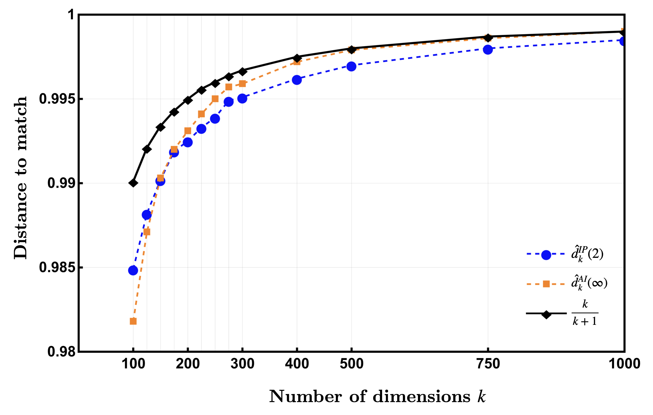
Figure 2. This figure reports estimates of $d^{\text{IP}}_{k}(2)$ and $d^{\text{AI}}_{k}(n)$ for $\sigma^{2}=0.05$ and $n=10,000$, using their average values over 1,000 draws. The quantity $d^{\text{AI}}_{k}(n)$ is initially below $d^{\text{IP}}_{k}(2)$ and eventually overtakes it. Both $d^{\text{IP}}_{k}(2)$ and $d^{\text{AI}}_{k}(n)$ converge to $k/(k+1)$ from below.

The practical relevance of Theorem 4.1 depends on whether capturing the full complexity of a person is necessary for identifying a good match. There are several reasons why the effective dimensionality might be smaller. First, for some individuals, compatibility may depend primarily on a few critical attributes—such as shared religious affiliation, similar educational background, or aligned political views. In this case, a small subset of core dimensions may suffice to determine match quality. Second, if the many attributes of personality are not independent but instead exhibit significant correlation, then the high-dimensional space of people may be approximable by a lower-dimensional space. For either of these reasons, small $k$ may be relevant. Nevertheless, Theorem 4.1 suggests that for individuals who truly value alignment across a large number of traits that are not inherently predictable from one another, search on an AI platform has limited value.

4.1. Discussion

Several aspects of the model are discussed below.

4.1.1. The role of the parametric assumptions.

In my model, personalities are uniformly distributed within a unit ball and AI errors follow a multivariate Gaussian distribution. While these parametric assumptions are important for the rate of convergence results behind Theorem 4.1, the core forces behind this theorem are more general. In particular, the key statistical phenomenon—that in high dimensions random points isolate from one another, and the distances between them concentrate around their expectations—holds across a broad range of distributional settings. This suggests that the conclusion of Theorem 4.1 may extend qualitatively (if not exactly) under other parametric assumptions. The other main result, Proposition 4.1, extends much more generally, holding for any nondegenerate distributions for the personality vectors and noise terms.

4.1.2. Two-sided matching

This paper’s model of search is one-sided, and thus abstracts from the question of whether Subject’s best match (once identified) would agree to this pairing. Although I do not pursue a complete strategic model in the present paper, in many reasonable formulations of such a model Subject’s expected payoff would decrease in the number of candidates considered by Subject’s potential partners. This effect would further favor the in-person regime, where each individual searches over fewer candidates, and thus strengthen the current results.

4.1.3. Increasingly accurate AI

Section 4 reveals a limitation of the AI representation regime that persists regardless of the quality of AI approximation (i.e., the size of the noise parameter $\sigma$). Nevertheless, we might expect that as the AI clones become more accurate representations of their underlying users, the AI representation regime will become more attractive relative to the in-person regime. In the appendix, I show that for every fixed dimension $k$, the quantity $d^{AI}_{k,\sigma}(\infty)$ (where the noise level $\sigma$ is now made explicit) converges to zero as $\sigma\rightarrow 0$. That is, Subject’s expected distance to Subject’s best match converges to zero as the AI’s approximation errors vanish. This means that while the value to increasing the size of the AI platform is capped, the value to increasing the accuracy of the AI clones is not.

4.1.4. Other utility functions

The Subject in my model prefers to match with similar individuals. While similarity is an important determinant of compatibility (Byrne and Nelson, 1964; Banikiotes and Neimeyer, 1981; Montoya et al., 2008), it is clearly not the full story. For example, a person might seek a partner whose traits contrast with or complement their own. All of the results in this paper are preserved if we interpret the axis as ordered such that the most preferred values of the trait are closer to the center. In particular, an “opposites attract” preference would map the value $x_{i}$ to

$$\pi(x_{i})=\left\{\begin{array}[]{cc}1-x_{i}&\mbox{ if }x_{i}\geq 0\\ -1-x_{i}&\mbox{ if }x_{i}<0\end{array}\right.$$

More substantial relaxations of this assumption—e.g., to non-uniform weighting over the attributes (such as $-\|wX_{i}\|$ for some weight vector $w$) or to nonlinear preferences (such as threshold functions over attributes)—would be interesting to consider, and are left to future work.

5. Heterogeneous Data Quantities

The remainder of the paper explores heterogeneity in the AI’s ability to mimic different individuals. In particular, not all individuals have the same amount of personal data to share with AI (e.g., because of variation in social media usage) or the same willingness to share it (e.g., because of variation in privacy preferences). These discrepancies will affect the AI’s ability to accurately represent each person.

In this extension, individuals belong to either of two groups: a “data-rich” group in which the estimation error is smaller, $\sigma^{2}_{\ell}$, and a “data-poor” group in which the estimation error is larger, $\sigma^{2}_{h}$. Proposition 5.1 says that in this world we will see a fundamental inequality emerge between people who are better and worse understood by the AI. In particular, although the groups are otherwise identical in distribution—and thus, ex-ante, Subject’s best match should be equally likely to be of either group, the probability that Subject is matched to someone in the data-rich group strictly exceeds $1/2$. This probability further converges to 1 as either the number of dimensions grows large (Corollary 5.1) or the ratio of noise variances grows large (Corollary 5.2).

In more detail, the population is equally split into two groups, where the data-rich group includes individuals indexed $i=1,\dots,n$ and the data-poor group includes individuals indexed $i=n+1,\dots,2n$. The AI clone of an individual from the data-rich group is

$$Y_{i0}=X_{i}+\varepsilon_{i0}^{\ell},\quad\quad\varepsilon_{i0}^{\ell}\sim\mathcal{N}(0,\sigma_{\ell}^{2}I_{k})$$

while the AI clone of an individual from the data-poor group is

$$Y_{i0}=X_{i}+\varepsilon_{i0}^{h},\quad\quad\varepsilon_{i0}^{h}\sim\mathcal{N}(0,\sigma_{h}^{2}I_{k})$$

where $\sigma_{h}>\sigma_{\ell}$. Subject may belong to either group, and as before is matched to the individual with index

$$i^{*}_{n}=\operatorname*{arg\,min}_{1\leq i\leq 2n}\|Y_{i0}-Y_{0i}\|,$$

i.e., the individual whose AI clone is most compatible with Subject’s AI clone.

Definition 5.1.

Let

$$g^{R}_{k}(0)=\frac{1}{V_{1,k}}\frac{1}{(4\pi\sigma_{\ell}^{2})^{k/2}}\int_{x\in B_{k}}\exp\left(-\frac{\|x\|^{2}}{4\sigma_{\ell}^{2}}\right)dx$$

and

$$g_{k}^{P}(0)=\frac{1}{V_{1,k}}\frac{1}{(2\pi(\sigma_{\ell}^{2}+\sigma_{h}^{2}))^{k/2}}\int_{x\in B_{k}}\exp\left(-\frac{\|x\|^{2}}{2(\sigma_{\ell}^{2}+\sigma_{h}^{2})}\right)dx$$

where $V_{1,k}=\frac{\pi^{k/2}}{\Gamma\left(\frac{k}{2}+1\right)}$ is the volume of the unit ball in $k$ dimensions. These quantities are the densities at zero of the random variable $\|Y_{i0}-Y_{0i}\|$ for, respectively, $i\leq n$ and $i>n$ (see the proof of Proposition 5.1 for details).

The next result says that as the population grows large, the probability with which Subject is matched to an individual from either group is proportional to that group’s density at zero. Whenever $\sigma_{h}>\sigma_{\ell}$, the probability that Subject’s best match is from the data-rich group is strictly greater than $1/2$.

Proposition 5.1.

In the limit as the population grows large, the probability that Subject’s match is from the data-rich group converges to

$$\lim_{n\rightarrow\infty}P(i_{n}^{*}<n)=\frac{g^{R}_{k}(0)}{g^{R}_{k}(0)+g^{P}_{k}(0)}\geq\frac{1}{2}.$$

This means that—even though individuals from the data-rich group and data-poor group are identical in distribution (both are drawn uniformly at random from the unit ball)—a data-rich individual is more likely to be identified as Subject’s best match. The following corollaries show that this inequality is exaggerated in either of two limits: as the dimension $k$ grows large or as the ratio $\sigma_{h}/\sigma_{\ell}$ grows large. In both cases, the probability that a data-rich individual is selected converges to 1.

Corollary 5.1 (Many Dimensions).

In the limit as the dimension and population both grow large, the probability that Subject’s match is from the data-rich group converges to 1, i.e.,

$$\lim_{k\rightarrow\infty}\left(\lim_{n\rightarrow\infty}P(i_{n}^{*}<n)\right)=1.$$

Corollary 5.2 (Large Noise Disparity).

Write $i_{n}^{*}(\alpha)$ for the (random) best-match individual when the data-rich and data-poor groups are governed, respectively, by $\sigma_{h}=\alpha\sigma$ and $\sigma_{\ell}=\sigma$ for some fixed $\sigma$. Then

$$\lim_{\alpha\rightarrow\infty}\left(\lim_{n\rightarrow\infty}P(i_{n}^{*}(\alpha)<n)\right)=1.$$

This systematic selection of data-rich individuals is beneficial for Subject. Indeed, holding fixed a distance between Subject’s clone and the best match AI clone, the expected true distance between Subject and this individual is smaller when the individual is from the data-rich group, since individuals in the data-rich group are better approximated by their AI clones.

The possibly harmful welfare consequences are for those being chosen. Since the results in this section do not depend on any special properties of Subject, they imply that individuals who are better understood by AI systems will be more in demand in general. This advantage may amplify existing social disparities, as groups with greater digital access and online presence are likely to be better represented in training data. They moreover point to a new form of social stratification: in a future with AI clones, an individual’s prospects may depend not just on their qualities, but also on how well AI systems can capture and interpret those qualities.

6. Conclusion

Many papers have compared human and AI evaluation on tasks that are hard for both humans and machines. But there are important evaluations that are intrinsically easier for people—for example, no machine or expert knows better than ourselves whose company we enjoy. In such settings, human evaluation is necessarily more accurate than the AI evaluation, but also more costly. Can automated search over a sufficiently large number of candidates compensate for the AI’s errors during evaluation? This paper suggests that the answer depends on the complexity of the target: When search is conducted over a set of highly complex options (such as people), the answer is no.

Appendix A Details on Figure 2

Table 1 provides the values $\hat{d}^{\text{IP}}_{k}(2)$, $\hat{d}^{\text{AI}}_{k}(\infty)$, and $\frac{k}{k+1}$ depicted in Figure 2, as well as estimates for additional values of $k$. For small values of $k$, $\hat{d}_{k}^{\text{AI}}(\infty)<\hat{d}^{\text{IP}}_{k}(2)$; indeed, for each of $k=1,5,10$, the expected distance to the AI best match is substantially lower than the expected distance to the in-person best match. This order reverses when the number of dimensions is large (in this case, 150 or larger). Finally, both quantities approach $k/(k+1)$ as $k$ grows large.

$k$	$\hat{d}^{\text{IP}}_{k}(2)$	$\hat{d}^{\text{AI}}_{k}(\infty)$	$\frac{k}{k+1}$
1	0.3346	0.0551	0.5
5	0.7554	0.1743	0.8333
10	0.8675	0.3664	0.9091
50	0.9709	0.9126	0.9804
100	0.9849	0.9818	0.9901
125	0.9882	0.9871	0.9921
150	0.9902	0.9903	0.9934
175	0.9919	0.9920	0.9943
200	0.9925	0.9931	0.9950
225	0.9933	0.9941	0.9956
250	0.9939	0.9950	0.9960
275	0.9949	0.9957	0.9964
300	0.9951	0.9959	0.9967
400	0.9962	0.9972	0.9975
500	0.9970	0.9979	0.9980
750	0.9980	0.9986	0.9987
1000	0.9985	0.9990	0.9990

Table 1. We set $\sigma^{2}=0.05$ and $n=10,000$ and estimate $d^{\text{IP}}_{k}(2)$ and $d^{\text{AI}}_{k}(n)$ using their average values over 1,000 draws. The cell with the smallest value is highlighted in gray.

Appendix B Proofs of the Main Results

The organization of this appendix is as follows. Appendix B.1 and Appendix B.2 present key supporting results about search in the in-person and AI representation regimes. Appendix B.3 completes the proof of Proposition 4.1, and Appendix B.4 completes the proof of Theorem 4.1.

B.1. Supporting Results about the In-Person Regime

Lemma B.1 provides a closed-form expression for $d^{\text{IP}}_{k}(m)$, Subject’s expected payoff in the in-person regime given $m$ samples. Lemma B.2 uses this result to bound the distance between $d^{\text{IP}}_{k}(2)$ and the benchmark $k/(k+1)$.

Lemma B.1.

For every number of dimensions $k$ and sample size $m$, Subject’s expected payoff in the in-person regime is

$$d^{\text{IP}}_{k}(m)=E\left[\min_{1\leq i\leq m}\|X_{i}\|\right]=\frac{1}{k}B\left(\frac{1}{k},m+1\right)$$

where $B$ denotes the Beta function.

Proof.

First observe that

$$P\left(\min_{1\leq i\leq m}\|X_{i}\|>r\right) =P\left(\|X_{1}\|>r\right)^{m} X_{i}$$ since are i.i.d.

$$=\left(1-\frac{V_{r,k}}{V_{1,k}}\right)^{m}=(1-r^{k})^{m}$$

where $V_{r,k}=\frac{\pi^{k/2}r^{k}}{\Gamma\left(\frac{k}{2}+1\right)}$ is the volume of a ball with radius $r$. Thus

$$E\left[\min_{1\leq i\leq m}\|X_{i}\|\right] =\int_{0}^{1}P\left(\min_{1\leq i\leq m}\|X_{i}\|>r\right)dr$$

$$=\int_{0}^{1}(1-r^{k})^{m}dr$$

$$=\frac{1}{k}B\left(\frac{1}{k},m+1\right)$$

as desired. ∎

Lemma B.2.

For every number of dimensions $k$,

(B.1) $$d^{\text{IP}}_{k}(2)=d^{\text{IP}}_{k}(1)-\frac{k}{(2k+1)(k+1)}=\frac{k}{k+1}-\frac{k}{(2k+1)(k+1)}.$$

Proof.

Since Lemma B.1 implies $d^{\text{IP}}_{k}(2)=\frac{1}{k}B\left(\frac{1}{k},3\right)$, it is equivalent to show

$$\frac{1}{k}B\left(\frac{1}{k},3\right)=\frac{k}{k+1}-\frac{k}{(2k+1)(k+1)}.$$

First simplify

$$\frac{1}{k}B\left(\frac{1}{k},3\right) =\frac{1}{k}\frac{\Gamma\left(\frac{1}{k}\right)\Gamma(3)}{\Gamma\left(\frac{1}{k}+3\right)}$$ by definition of the Beta function

$$=\frac{1}{k}\frac{2\Gamma\left(\frac{1}{k}\right)}{\Gamma\left(\frac{1}{k}+3\right)} \Gamma(3)=2!$$ since

$$=\frac{1}{k}\frac{2\Gamma\left(\frac{1}{k}\right)}{\left(\frac{1}{k}+2\right)\left(\frac{1}{k}+1\right)\frac{1}{k}\Gamma\left(\frac{1}{k}\right)}$$ by the Gamma function recurrence relation

$$=\frac{2k^{2}}{(2k+1)(k+1)}$$

Since

$$\frac{k}{k+1}-\frac{k}{(2k+1)(k+1)}=\frac{2k^{2}}{(2k+1)(k+1)}$$

we have the desired equality

$$\frac{1}{k}B\left(\frac{1}{k},3\right)=\frac{k}{k+1}-\frac{k}{(2k+1)(k+1)}.$$

We can similarly simplify

$$\frac{1}{k}B\left(\frac{1}{k},2\right) =\frac{1}{k}\frac{\Gamma\left(\frac{1}{k}\right)\Gamma(2)}{\Gamma\left(\frac{1}{k}+2\right)}=\frac{1}{k}\frac{\Gamma\left(\frac{1}{k}\right)}{\Gamma\left(\frac{1}{k}+2\right)}=\frac{1}{k}\frac{\Gamma\left(\frac{1}{k}\right)}{\left(\frac{1}{k}+1\right)\frac{1}{k}\Gamma\left(\frac{1}{k}\right)}=\frac{k}{k+1}$$

so also $d^{\text{IP}}_{k}(2)=d^{\text{IP}}_{k}(1)-\frac{k}{(2k+1)(k+1)}$, i.e., the expected marginal benefit of the second in-person draw is a reduction in the distance between Subject and Subject’s match by $\frac{k}{(2k+1)(k+1)}$. ∎

B.2. Supporting Results about the AI Representation Regime

I prove the following supporting results: First, Subject’s expected distance to individual $i$ is increasing in the distance between their AI clones (Lemma B.3). Thus for every finite $n$, Subject’s expected payoff can be upper bounded by Subject’s payoff in an idealized setting where some AI clone perfectly matches Subject’s AI clone, henceforth denoted $d^{\text{AI}}_{k}(\infty)$ (Corollary B.1). Lemma B.4 proves that $d^{\text{AI}}_{k}(\infty)$ is equal to the expectation of the norm of a multivariate Gaussian vector, conditional on that norm being less than 1. Finally, Proposition B.5 asymptotically bounds the difference between $d^{\text{AI}}_{k}(\infty)$ and the benchmark distance $k/(k+1)$, and Lemma B.6 shows that $d^{\text{AI}}_{k}(\infty)<k/(k+1)$ for every $k$.

Lemma B.3.

$\mathbb{E}[\|X_{i}\|:\|Y_{i0}-Y_{0i}\|=s]$ is increasing in $s$.

Proof.

Fix an arbitrary individual $i$ and define $Z_{i}\equiv\varepsilon_{i0}-\varepsilon_{0i}\sim\mathcal{N}(0,2\sigma^{2}I_{k})$. Let $R\equiv\|X\|$ and $S\equiv\|X+Z\|$, where I drop the $i$ subscript to ease notation. I will show that the joint density $f_{R,S}$ satisfies the monotone likelihood ratio property, i.e.,

(B.2) $$f_{R,S}(r,s)\,f_{R,S}(r^{\prime},s^{\prime})>f_{R,S}(r,s^{\prime})\,f_{R,S}(r^{\prime},s)$$

for every $1\geq r>r^{\prime}\geq 0$ and $s>s^{\prime}\geq 0$. It is well known that (B.2) implies that $E(R\mid S=s)$ is increasing in $s$ (see e.g., Milgrom (1981)).

Towards demonstrating (B.2), I will first derive a closed-form expression for each of $f_{R}(r)$ and $f_{S\mid R=r}(s)$. Since $X$ is uniformly distributed on the unit ball, its norm $R$ has distribution function

$$F_{R}(r)=\mathbb{P}(R\leq r)=\frac{V_{r,k}}{V_{1,k}}=r^{k}\quad\forall r\in[0,1]$$

where $V_{r,k}=\frac{\pi^{k/2}r^{k}}{\Gamma\left(\frac{k}{2}+1\right)}$ is the volume of a ball with radius $r$. Differentiating yields

(B.3) $$f_{R}(r)=k\,r^{k-1}\quad\forall r\in[0,1].$$

Next turn to $f_{S|R=r}$. Conditional on $R=r$, we can write $X=r\,u$ for some unit vector $u$ in the $k$-dimensional unit sphere. Hence

$$S=\|X+\varepsilon\|=\|r\,u+\varepsilon\|$$

where the direction $u$ is irrelevant for the distribution of $S$.

Define $T=\frac{S}{\sigma}$. Then $T\mid(R=r)=\|\frac{rU}{\sigma}+\frac{\varepsilon}{\sigma}\|$ has a noncentral chi distribution with dimension $k$ and mean vector $\mu=\frac{ru}{\sigma}$. The pdf for such a distribution is known to be

(B.4) $$f_{T}(t)=\frac{1}{\lambda^{\nu}}t^{\nu}\exp\left[-\frac{t^{2}+\lambda^{2}}{2}\right]I_{\nu}(\lambda t)$$

where $\lambda=\|\mu\|=\frac{r}{\sigma}$, $\nu=\frac{k}{2}-1$, and $I_{\nu}$ is the modified Bessel function of the first kind.

Applying the change of variable $S=\sigma T$ we have

$$f_{S}(s)=\frac{1}{\sigma}\;f_{T}\left(\frac{s}{\sigma}\right),\quad s\geq 0.$$

and thus (plugging in (B.4) with $t=s/\sigma$),

$$f_{S}(s)=\frac{1}{\sigma}\left(\frac{s}{r}\right)^{\nu}\exp\left[-\frac{r^{2}+s^{2}}{2\sigma^{2}}\right]I_{k/2-1}\left(\frac{r\,s}{\sigma^{2}}\right).$$

Together with (B.3) this yields

$$f_{R,S}(r,s) =\left(k\,r^{\,k-1}\right)\cdot\left(\frac{1}{\sigma}\left(\frac{s}{r}\right)^{k/2-1}\exp\left[-\frac{r^{2}+s^{2}}{2\sigma^{2}}\right]I_{\frac{k}{2}-1}\left(\frac{r\,s}{\sigma^{2}}\right)\right)$$

$$=\frac{k}{\sigma}\cdot\left(r^{k/2}s^{k/2-1}\exp\left[-\frac{r^{2}+s^{2}}{2\sigma^{2}}\right]I_{\frac{k}{2}-1}\left(\frac{r\,s}{\sigma^{2}}\right)\right)$$

A sufficient condition for (B.2) is for the function $f_{R,S}$ to be log-supermodular (Athey, 2002). Thus define

$$\phi(r,s) =\ln f_{R,S}(r,s)$$

(B.5) $$=\ln\frac{k}{\sigma}+\frac{k}{2}\ln(r)+\left(\frac{k}{2}-1\right)\ln(s)-\frac{r^{2}+s^{2}}{2\sigma^{2}}+\ln\left(I_{\frac{k}{2}-1}\left(\frac{r\,s}{\sigma^{2}}\right)\right).$$

Since only the final term of (B.5) has a nonzero cross-partial,

$$\frac{\partial^{2}}{\partial r\,\partial s}\phi(r,s)=\frac{\partial^{2}}{\partial r\partial s}\ln\left(I_{\frac{k}{2}-1}\left(\frac{rs}{\sigma^{2}}\right)\right)$$

Let $z=r\,s/\sigma^{2}$ and again denote $\nu=\frac{k}{2}-1$. Then

$$\frac{\partial}{\partial r}\ln I_{\nu}(z)=\frac{I_{\nu}^{\prime}(z)}{I_{\nu}(z)}\cdot\frac{s}{\sigma^{2}}$$

and so

$$\frac{\partial^{2}}{\partial r\partial s}\ln\left(I_{\nu}\left(\frac{rs}{\sigma^{2}}\right)\right)=\frac{\partial}{\partial s}\left[\frac{I_{\nu}^{\prime}(z)}{I_{\nu}(z)}\cdot\frac{s}{\sigma^{2}}\right] =\frac{\partial}{\partial s}\left[\frac{I_{\nu}^{\prime}(z)}{I_{\nu}(z)}\right]\cdot\frac{s}{\sigma^{2}}+\frac{I_{\nu}^{\prime}(z)}{I_{\nu}(z)}\cdot\frac{1}{\sigma^{2}}$$

$$=\frac{\partial}{\partial z}\left[\frac{I_{\nu}^{\prime}(z)}{I_{\nu}(z)}\right]\cdot\frac{rs}{\sigma^{4}}+\frac{I_{\nu}^{\prime}(z)}{I_{\nu}(z)}\cdot\frac{1}{\sigma^{2}}$$

We can now sign the RHS using properties of $I_{\nu}$, the modified Bessel function of the first kind (see e.g., Árpád Baricz (2010)). First, $I_{\nu}^{\prime}(z)\geq 0$ and $I_{\nu}(z)\geq 0$ for all $z\geq 0$ (which is implied by $r,s\geq 0$); thus, $\frac{I_{\nu}^{\prime}(z)}{I_{\nu}(z)}\geq 0$. Moreover, for $\nu\geq-1/2$ (which is satisfied in our setting since $k\geq 1$), the function $I_{\nu}$ is log-convex on $(0,\infty)$, i.e., $\frac{d}{dz}\left[\frac{I_{\nu}^{\prime}(z)}{I_{\nu}(z)}\right]\geq 0$. Thus the entire RHS is positive, so $f(r,s)=\exp(\phi(r,s))$ is log-supermodular as desired. ∎

Corollary B.1.

Define $d^{\text{AI}}_{k}(\infty)=\mathbb{E}\left[\|X_{i}\|:\|Y_{i0}-Y_{0i}\|=0\right].$ Then $d^{\text{AI}}_{k}(\infty)\leq d^{\text{AI}}_{k}(n)$ for all $n\in\mathbb{Z}_{+}.$

Proof.

Define $W=\min_{1\leq j\leq n}\|Y_{j0}-Y_{0j}\|$. Then

$$d_{k}^{\text{AI}}(n)=E\left[\|X_{i}\|:\|Y_{i0}-Y_{0i}\|=W\right]$$

where clearly $P(W\geq 0)=1$. So

$$d_{k}^{\text{AI}}(n)\geq E\left[\|X_{i}\|:\|Y_{i0}-Y_{0i}\|=0\right]$$

follows by Lemma D.1. ∎

Lemma B.4.

For each $i$, $E\left[\|X_{i}\|:\|Y_{i0}-Y_{0i}\|=0\right]=E[\|Z\|:\|Z\|\leq 1|]$ where $Z\sim\mathcal{N}(0,2\sigma^{2}I_{k})$ and $I_{k}$ is the identity matrix in $k$ dimensions.

Proof.

Recall that $Y_{i0}=Y_{0i}$ is equivalent to $X_{i}+\varepsilon_{i0}=x_{0}+\varepsilon_{0i}$, or more simply

$$X_{i}=Z_{i}$$

where $Z_{i}=\varepsilon_{0i}-\varepsilon_{i0}\sim\mathcal{N}(0,2\sigma^{2}I_{k})$. By Bayes’ rule, the posterior density of $X_{i}$ conditional on the event $\{X_{i}=Z_{i}\}$ satisfies

$$f_{X_{i}|Z_{i}=X_{i}}(x)=\frac{f_{X_{i}}(x)f_{Z_{i}}(x)}{\int_{x\in B_{k}}f_{X_{i}}(x)f_{Z_{i}}(x)dx}$$

Since $f_{X_{i}}(x)$ is constant on $B_{k}$ and zero elsewhere, this further simplifies to

$$f_{X_{i}|Z_{i}=X_{i}}(x)=\frac{f_{Z_{i}}(x)}{\int_{x\in B_{k}}f_{Z_{i}}(x)dx}$$

That is, $X_{i}\mid(Y_{i0}=Y_{0i})\stackrel{{\scriptstyle d}}{{=}}Z_{i}\mid\{\|Z_{i}\|\leq 1\}$ which further implies

$$E[\|X_{i}\|:Y_{i0}=Y_{0i}]=E[\|Z_{i}\|:\|Z_{i}\|\leq 1]$$

as desired. ∎

Lemma B.5.

$d^{\text{AI}}_{k}(\infty)=\frac{k}{k+1}+o\left(\frac{1}{k}\right)$

Proof.

Let $Z\sim N(0,2\sigma^{2}I_{k})$, and define $R=\|Z\|$. Then $\frac{R^{2}}{2\sigma^{2}}$ has a chi-squared distribution with parameter $k$. Applying the change of variable $X=\frac{R^{2}}{2\sigma^{2}}$ (or equivalently, $R=\sqrt{2\sigma^{2}X}$) we obtain the standard expression for the probability density function of $R$,

(B.6) $$f_{R}(r)=\frac{2^{1-\frac{k}{2}}}{\Gamma(\frac{k}{2})\sigma^{k}}r^{k-1}\exp\left(-\frac{r^{2}}{4\sigma^{2}}\right)\quad\forall r\geq 0.$$

Thus

$$\mathbb{E}[R\mid R\leq 1]=\frac{\int_{0}^{1}rf^{R}(r)dr}{\int_{0}^{1}f^{R}(r)dr}=\frac{\int_{0}^{1}r^{k}\exp\left(-\frac{r^{2}}{4\sigma^{2}}\right)dr}{\int_{0}^{1}r^{k-1}\exp\left(-\frac{r^{2}}{4\sigma^{2}}\right)dr}$$

and the desired result follows from demonstrating

(B.7) $$\frac{\int_{0}^{1}r^{k}\exp\left(-\frac{r^{2}}{4\sigma^{2}}\right)dr}{\int_{0}^{1}r^{k-1}\exp\left(-\frac{r^{2}}{4\sigma^{2}}\right)dr}=\frac{k}{k+1}+o\left(\frac{1}{k}\right).$$

For each positive integer $k$, define

$$I_{1}(k):=\int_{0}^{1}r^{k}\exp\left(-\frac{r^{2}}{4\sigma^{2}}\right)dr\quad\text{and}\quad I_{2}(k):=\int_{0}^{1}r^{k-1}\exp\left(-\frac{r^{2}}{4\sigma^{2}}\right)dr.$$

For any $\delta\in(0,1)$, we can split the integral as

(B.8) $$I_{1}(k)=\int_{0}^{1-\delta}r^{k}\exp\left(-\frac{r^{2}}{4\sigma^{2}}\right)dr+\int_{1-\delta}^{1}r^{k}\exp\left(-\frac{r^{2}}{4\sigma^{2}}\right)dr$$

On the domain $[0,1-\delta]$, we have $r^{k}\leq(1-\delta)^{k}$ and $\exp\left(-\frac{r^{2}}{4\sigma^{2}}\right)\leq 1$, so

$$\int_{0}^{1-\delta}r^{k}\exp\left(-\frac{r^{2}}{4\sigma^{2}}\right)dr\leq\int_{0}^{1-\delta}r^{k}dr=\frac{(1-\delta)^{k+1}}{k+1}$$

Now consider the second term in (B.8). Note that

$$e^{-\frac{r^{2}}{4\sigma^{2}}}=e^{-\frac{1}{4\sigma^{2}}}+\Delta(r)\quad\mbox{where }\Delta(r)=e^{-\frac{r^{2}}{4\sigma^{2}}}-e^{-\frac{1}{4\sigma^{2}}}.$$

Because $r\leq 1$, the function $\Delta(r)$ is nonnegative and can be bounded

$$0\leq\Delta(r)\leq c(\delta)\quad\mbox{for }r\in[1-\delta,1]$$

where

$$c(\delta)=\exp\left(-\frac{(1-\delta)^{2}}{4\sigma^{2}}\right)-\exp\left(-\frac{1}{4\sigma^{2}}\right).$$

Thus

$$\int_{1-\delta}^{1}r^{k}\exp\left(-\frac{r^{2}}{4\sigma^{2}}\right)dr=\exp\left(-\frac{1}{4\sigma^{2}}\right)\int_{1-\delta}^{1}r^{k}dr+\int_{1-\delta}^{1}r^{k}\Delta(r)dr$$

where

$$\exp\left(-\frac{1}{4\sigma^{2}}\right)\,\int_{1-\delta}^{1}r^{k}dr=\exp\left(-\frac{1}{4\sigma^{2}}\right)\left(\frac{1}{k+1}-\frac{(1-\delta)^{k+1}}{k+1}\right)$$

while

$$0\leq\int_{1-\delta}^{1}r^{k}\Delta(r)dr\leq c(\delta)\int_{1-\delta}^{1}r^{k}dr=c(\delta)\left(\frac{1}{k+1}-\frac{(1-\delta)^{k+1}}{k+1}\right).$$

Putting these bounds together yields

$$\left|I_{1}(k)-\frac{\exp\left(-\frac{1}{4\sigma^{2}}\right)}{k+1}\right|\leq\frac{(1-\delta)^{k+1}}{k+1}\left(1+\exp\left(-\frac{1}{4\sigma^{2}}\right)\right)+\frac{c(\delta)}{k+1}.$$

Since $\delta$ can be chosen arbitrarily in $(0,1)$, we now set $\delta_{k}=\frac{\ln k}{k}$, which tends to $0$ as $k\to\infty$ but still satisfies $(1-\delta_{k})^{k+1}=\frac{1}{k}+o\left(\frac{1}{k}\right)$. Hence

$$\frac{(1-\delta_{k})^{k+1}}{k+1}=O\left(\frac{1}{k^{2}}\right)=o\left(\frac{1}{k}\right),\quad\text{and}\quad\frac{c(\delta_{k})}{k+1}=o\left(\frac{1}{k}\right).$$

It follows that

$$I_{1}(k)=\frac{\exp\!\left(-\frac{1}{4\sigma^{2}}\right)}{k+1}+o\left(\frac{1}{k}\right).$$

By identical reasoning (replacing $k$ by $k-1$), we obtain

$$I_{2}(k)=\int_{0}^{1}r^{k-1}\exp\left(-\frac{r^{2}}{4\sigma^{2}}\right)dr=\frac{\exp\!\left(-\frac{1}{4\sigma^{2}}\right)}{k}+o\left(\frac{1}{k}\right).$$

Combining the two asymptotic expansions,

$$\frac{I_{1}(k)}{I_{2}(k)}=\frac{\frac{1}{k+1}e^{-\frac{1}{4\sigma^{2}}}+o\left(\frac{1}{k}\right)}{\frac{1}{k}e^{-\frac{1}{4\sigma^{2}}}+o\left(\frac{1}{k}\right)}=\frac{k}{k+1}+o\left(\frac{1}{k}\right)$$

as desired. ∎

Lemma B.6.

For every positive integer $k$, $d^{\text{AI}}_{k}(\infty)<\frac{k}{k+1}+o\left(\frac{1}{k}\right).$

Proof.

Let $T$ be the random variable with density function

$$f_{T}(r)=\frac{r^{k}\exp\left(-\frac{r^{2}}{4\sigma^{2}}\right)}{\int_{0}^{1}r^{k-1}\exp\left(-\frac{r^{2}}{4\sigma^{2}}\right)dr}$$

on $[0,1]$, observing that

$$E[T]=d_{k}^{\text{AI}}(\infty)=\frac{\int_{0}^{1}r^{k}\exp\left(-\frac{r^{2}}{4\sigma^{2}}\right)dr}{\int_{0}^{1}r^{k-1}\exp\left(-\frac{r^{2}}{4\sigma^{2}}\right)dr}.$$

Consider also a Beta$(k,1)$ random variable $B$, whose density function on $[0,1]$ is $f_{B}(r)=kr^{k-1}$ and expectation is $E[B]=\frac{k}{k+1}.$ The likelihood ratio

$$\frac{f_{T}(r)}{f_{B}(r)}=\frac{1}{kr^{k-1}}\frac{r^{k-1}\exp\left(-\frac{r^{2}}{4\sigma^{2}}\right)}{\int_{0}^{1}r^{k-1}\exp(-r^{2}/4\sigma^{2})dr}=\frac{1}{k}\frac{\exp(-r^{2}/4\sigma^{2})}{\int_{0}^{1}r^{k-1}\exp(-r^{2}/4\sigma^{2})dr}.$$

is strictly decreasing in $r$, implying that $\left\{\frac{f_{R}(r)}{f_{B}(r)}\right\}_{r\geq 0}$ has the monotone likelihood ratio property. Thus the distribution of $B$ first-order stochastically dominates the distribution of $T$, implying in particular that $E[T]<E[B]$, or equivalently,

$$\frac{\int_{0}^{1}r^{k}\exp\left(-\frac{r^{2}}{4\sigma^{2}}\right)dr}{\int_{0}^{1}r^{k-1}\exp\left(-\frac{r^{2}}{4\sigma^{2}}\right)dr}<\frac{k}{k+1}$$

as desired.∎

B.3. Proof of Proposition 4.1

By Lemma B.1,

$$d^{\text{IP}}_{k}(m)=\frac{1}{k}B\left(\frac{1}{k},m+1\right)$$

For every fixed $k$, this expression converges to zero as $m$ grows large. Since

$$\mathbb{E}\left[\|X_{i}\|:\|Y_{i0}-Y_{0i}\|=0\right]>0$$

we can identify a finite $m$ such that

$$d^{\text{IP}}_{k}(m)<\mathbb{E}\left[\|X_{i}\|:\|Y_{i0}-Y_{0i}\|=0\right].$$

Then by Corollary B.1,

$$d^{\text{IP}}_{k}(m)\leq d^{\text{AI}}_{k}(n)\quad\forall n\in\mathbb{Z}_{+}$$

implying that the AI equivalent sample size exists and is finite.

B.4. Proof of Theorem 4.1

By Lemma B.2,

$$d^{\text{IP}}_{k}(2)=\frac{k}{k+1}-\frac{k}{(2k+1)(k+1)}$$

where $\frac{k}{(2k+1)(k+1)}=\Theta\left(\frac{1}{k}\right)$. By Lemma B.5,

$$d^{\text{AI}}_{k}(\infty)=\frac{k}{k+1}+o\left(\frac{1}{k}\right)$$

and by Corollary B.1, this is a uniform lower bound on $d^{\text{AI}}_{k}(n)$ for all $n$. Thus when $k$ is sufficiently large, we have

$$d^{\text{IP}}_{k}(2)<d^{\text{AI}}_{k}(n)$$

for all $n\in\mathbb{Z}_{+}$. Finally, Lemmas B.2 and B.6 imply that

$$\frac{k}{k+1}=d^{\text{IP}}_{k}(1)>d^{\text{AI}}_{k}(n),$$

so $m=1$ does not satisfy $d^{\text{IP}}_{k}(m)<d^{\text{AI}}_{k}(n)$ for all $n$. Thus $m_{k}^{*}=2$ is the AI equivalent sample size for $k$ sufficiently large.

Appendix C Proofs of Results in Section 5

C.1. Proof of Proposition 5.1

I proceed under the assumption that Subject is estimated with low noise, i.e., $Y_{0i}=\varepsilon^{\ell}_{0i}\sim\mathcal{N}(0,\sigma_{\ell}^{2}I_{k})$, with the result holding by identical arguments if instead $Y_{0i}\sim\mathcal{N}(0,\sigma_{h}^{2}I_{k})$. For all individuals $i$, let $S_{i}=\|Y_{i0}-Y_{0i}\|$. Then for individuals in the low-noise group, i.e., $1\leq i\leq n$,

$$S_{i}=\|X_{i}+Z^{\ell}_{i}\|\quad\mbox{where}\quad Z^{\ell}_{i}=\varepsilon^{\ell}_{i0}-\varepsilon^{\ell}_{0i}\sim\mathcal{N}(0,2\sigma_{\ell}^{2}I_{k}).$$

Let $G^{R}$ denote the CDF of this variable. Since $X_{i}$ is drawn uniformly from the unit ball $B_{k}$, $G^{R}$ admits a continuous density $g^{R}$ that takes value

$$g^{R}(0)=\int_{x\in B_{k}}\frac{1}{V_{1,k}}\frac{1}{(4\pi\sigma_{\ell}^{2})^{k/2}}\exp\left(-\frac{\|x\|^{2}}{4\sigma_{\ell}^{2}}\right)dx$$

at zero. (As before $V_{1,k}$ denotes the volume of the unit ball in $k$ dimensions.)

For individuals in the data-poor group ($n+1\leq i\leq 2n$),

$$S_{i}=\|X_{i}+Z^{h}_{i}\|\quad\mbox{where}\quad Z^{h}_{i}=\varepsilon^{h}_{i0}-\varepsilon^{\ell}_{0i}\sim\mathcal{N}(0,(\sigma_{\ell}^{2}+\sigma_{h}^{2})I_{k}).$$

Let $G^{P}$ denote the distribution of this variable. By similar reasoning, $G^{P}$ admits a continuous density $g^{P}$ that takes value

$$g^{P}(0)=\int_{x\in B_{k}}\frac{1}{V_{1,k}}\frac{1}{(2\pi(\sigma_{\ell}^{2}+\sigma_{h}^{2}))^{k/2}}\exp\left(-\frac{\|x\|^{2}}{2(\sigma_{\ell}^{2}+\sigma_{h}^{2})}\right)dx$$

at the zero vector. Moreover $g^{R}(0)>g^{P}(0)$ by assumption that $\sigma_{h}>\sigma_{\ell}$.

The distance between Subject’s clone and the best match clone in, respectively, the data-rich and data-poor groups are $M_{n}^{R}=\min_{1\leq i\leq n}S_{i}$ and $M_{n}^{P}=\min_{n+1\leq i\leq 2n}S_{i}$. Let their respective distributions be denoted by $H^{R}$ and $H^{P}$. Then

$$H^{R}(s)=1-\left(1-G^{R}(s)\right)^{n}\quad\mbox{and}\quad H^{P}(s)=1-\left(1-G^{P}(s)\right)^{n}$$

with densities

$$h^{R}(s)=n\left(1-G^{R}(s)\right)^{n-1}g^{R}(s)\quad\mbox{and}\quad h^{P}(s)=n\left(1-G^{P}(s)\right)^{n-1}g^{P}(s)$$

Since $M_{n}^{R}$ and $M_{n}^{P}$ are independent,

$$P(M_{n}^{R}<M_{n}^{P}) =\int_{0}^{\infty}(1-H^{P}(s))dH^{R}(s)$$

$$=\int_{0}^{\infty}\left(1-G^{P}(s)\right)^{n}\left(n[1-G^{R}(s)]^{n-1}g^{R}(s)\right)ds.$$

Set $\alpha=g^{R}(0)+g^{P}(0)$ and apply the change of variable $t=n\alpha s$. Then

$$P(M_{n}^{R}<M_{n}^{P})=\frac{1}{\alpha}\int_{0}^{\infty}\left(1-G^{R}\left(\frac{t}{n\alpha}\right)\right)^{n-1}\left(1-G^{P}\left(\frac{t}{n\alpha}\right)\right)^{n}\,g^{R}\left(\frac{t}{n\alpha}\right)dt.$$

Denote the integrand by

$$I_{n}(t)=\left(1-G^{R}\left(\frac{t}{n\alpha}\right)\right)^{n-1}\left(1-G^{P}\left(\frac{t}{n\alpha}\right)\right)^{n}\,g^{R}\left(\frac{t}{n\alpha}\right)$$

so that $P(M_{n}^{R}<M_{n}^{P})=\frac{1}{\alpha}\int_{0}^{\infty}I_{n}(t)dt$.

Lemma C.1.

For each fixed $t>0$, $\lim_{n\to\infty}I_{n}(t)=g^{R}(0)e^{-t}.$

Proof.

Expanding $F$ around $s=0$, we have

$$G^{R}(s)=g^{R}(0)s+O(s^{2}),$$

Using the standard expansion $\ln(1-n)=-u+O(u^{2})$, we further obtain

$$\ln\left(1-G^{R}\left(\frac{t}{n\,\alpha}\right)\right)=-g^{R}(0)\frac{t}{n\alpha}+O\left(\frac{1}{n^{2}}\right).$$

Thus

$$(n-1)\ln\left(1-G^{R}\left(\frac{t}{n\,\alpha}\right)\right)=-g^{R}(0)\frac{t}{\alpha}+O\left(\frac{1}{n}\right),$$

implying

$$\left(1-G^{R}\left(\frac{t}{n\alpha}\right)\right)^{n-1} =\exp\left((n-1)\ln\left(1-G^{R}\left(\frac{t}{n\alpha}\right)\right)\right)$$

$$=\exp\left(-g^{R}(0)\frac{t}{\alpha}+O\left(\frac{1}{n}\right)\right)\longrightarrow e^{-g^{R}(0)\frac{t}{\alpha}}.$$

By identical reasoning,

$$\left(1-G^{P}\left(\frac{t}{n\alpha}\right)\right)^{n}\longrightarrow e^{-g^{P}(0)\frac{t}{\alpha}}.$$

Finally, $g^{R}\left(\frac{t}{n\alpha}\right)\rightarrow g^{R}(0)$ by continuity of $g^{R}$. Multiplying these limits yields

$$g^{R}(0)e^{-g^{R}(0)\frac{t}{\alpha}}e^{-g^{P}(0)\frac{t}{\alpha}}=g^{R}(0)e^{-\frac{t}{\alpha}(g^{R}(0)+g^{P}(0))}=g^{R}(0)e^{-t}$$

recalling that $\alpha=g^{R}(0)+g^{P}(0)$. Thus

$$I_{n}(t)=\left(1-G^{R}\left(\frac{t}{n\alpha}\right)\right)^{n-1}\left(1-G^{P}\left(\frac{t}{n\alpha}\right)\right)^{n}\,g^{R}\left(\frac{t}{n\alpha}\right)\longrightarrow g^{R}(0)e^{-t}$$

for each $t$, as desired. ∎

We next show that $I_{n}(t)$ is dominated by an integrable function so that we can apply the Dominated Convergence Theorem.

Lemma C.2.

There exists a function $D(t)$, independent of $n$, such that $I_{n}(t)\leq D(t)$ for all $n,t\geq 0$. Moreover, $\int_{0}^{\infty}D(t)\,dt<\infty$.

Proof.

Pick any $T>0$ and note that since both $G^{R}$ and $G^{P}$ have nonzero density at zero, $1-G^{R}(T)<1$ and $1-G^{P}(T)<1$. For each $n$, split the interval of integration into $[0,n\alpha T]$ and $(n\alpha T,\infty)$.

On the first interval, $s=\frac{t}{n\,\alpha}\in[0,T]$. Since $g^{R}$ is continuous (hence bounded) on $[0,T]$, there is a constant $\kappa_{1}$ with $f(x)\leq\kappa_{1}$ for all $x\in[0,T]$. Moreover, $[1-G^{R}(x)]^{n-1}\leq 1$ and $[1-G^{P}(x)]^{n}\leq 1$. Hence

$$I_{n}(t)=\left(1-G^{R}\left(\frac{t}{n\alpha}\right)\right)^{n-1}\left(1-G^{P}\left(\frac{t}{n\alpha}\right)\right)^{n}\,g^{R}\left(\frac{t}{n\alpha}\right)\leq\kappa_{1}$$

for all $0\leq t\leq n\alpha T$.

On the remaining interval, $s=\frac{t}{n\,\alpha}\geq T$. By monotonicity of the CDF, $1-G^{R}(s)\leq 1-G^{R}(T)$ and $1-G^{P}(s)\leq 1-G^{P}(T)$ for $s\geq T$. Define

$$c_{1}:=1-G^{R}(T)\quad\quad c_{2}:=1-G^{P}(T)$$

observing that $c_{1},c_{2}\in[0,1)$. Then

$$\left(1-F\left(\frac{t}{n\alpha}\right)\right)^{n-1}\leq c_{1}^{n-1}\quad\quad\left(1-G\left(\frac{t}{n\alpha}\right)\right)^{n}\leq c_{2}^{n}.$$

where $c_{1}^{n}$ and $c_{2}^{n}$ decay exponentially in $n$. Finally, since $g^{R}$ is obtained by convolving a bounded indicator function (the uniform distribution on the unit ball) with a Gaussian density, it is continuous and finite at every $r\in[0,\infty)$. Hence $g^{R}$ is bounded above by a global constant $\kappa_{2}$. Putting these arguments together,

$$I_{n}(t)\leq c_{1}^{n-1}c_{2}^{n}\kappa_{2}\leq ce^{-\beta t}\quad\forall\,t\geq n\alpha T$$

for some positive constant $\beta$. Clearly $\kappa_{2}ce^{-\beta t}$ is integrable over $[n\alpha T,\infty)$.

Combining these two bounds, define

$$D(t)=\max\left\{\kappa_{1},\kappa_{2}\,c\,e^{-\beta t}\right\}.$$

This function is integrable on $[0,\infty)$ and satisfies $I_{n}(t)\leq D(t)$ for all $n,t\geq 0$. ∎

We will now conclude the proof of Proposition 5.1. Recall that

$$\Pr(M_{n}^{R}<M_{n}^{H})=\frac{1}{\alpha}\int_{0}^{\infty}I_{n}(t)dt.$$

By Lemma C.2 and the Dominated Convergence Theorem,

$$\lim_{n\to\infty}\int_{0}^{\infty}I_{n}(t)dt=\int_{0}^{\infty}\lim_{n\to\infty}I_{n}(t)dt$$

And applying Lemma C.1 we have

$$\int_{0}^{\infty}\lim_{n\to\infty}I_{n}(t)dt=\int_{0}^{\infty}g^{R}(0)\,e^{-t}\,dt=g^{R}(0).$$

Hence,

$$\Pr(M_{n}^{R}<M_{n}^{H})=\frac{1}{\alpha}\int_{0}^{\infty}I_{n}(t)dt=\frac{1}{\alpha}g^{R}(0)=\frac{g^{R}(0)}{g^{R}(0)+g^{P}(0)}$$

as desired.

C.2. Proof of Corollary 5.1

From Proposition 5.1, we know that the limiting probability as the population grows large is

$$\lim_{n\rightarrow\infty}P(i_{n}^{*}<n)=\frac{g^{R}_{k}(0)}{g^{R}_{k}(0)+g^{P}_{k}(0)}=\left(\frac{\sigma_{\ell}^{2}+\sigma_{h}^{2}}{2\sigma_{\ell}^{2}}\right)^{k/2}\frac{\int_{x\in B_{k}}\exp\left(-\frac{\|x\|^{2}}{4\sigma_{\ell}^{2}}\right)dx}{\int_{x\in B_{k}}\exp\left(-\frac{\|x\|^{2}}{2(\sigma_{\ell}^{2}+\sigma_{h}^{2})}\right)dx}$$

Since $\sigma_{h}>\sigma_{\ell}$,

$$\left(\frac{\sigma_{\ell}^{2}+\sigma_{h}^{2}}{2\sigma_{\ell}^{2}}\right)^{k/2}\longrightarrow\infty\mbox{ as }k\rightarrow\infty$$

Moreover, for every $x\in B_{k}$,

$$\exp\left(-\frac{\|x\|^{2}}{4\sigma_{\ell}^{2}}\right)>\exp\left(-\frac{\|x\|^{2}}{2(\sigma_{\ell}^{2}+\sigma_{h}^{2})}\right)$$

so it follows that

$$\frac{\int_{x\in B_{k}}\exp\left(-\frac{\|x\|^{2}}{4\sigma_{\ell}^{2}}\right)dx}{\int_{x\in B_{k}}\exp\left(-\frac{\|x\|^{2}}{2(\sigma_{\ell}^{2}+\sigma_{h}^{2})}\right)dx}>1$$

Hence

$$\left(\frac{\sigma_{\ell}^{2}+\sigma_{h}^{2}}{2\sigma_{\ell}^{2}}\right)^{k/2}\frac{\int_{x\in B_{k}}\exp\left(-\frac{\|x\|^{2}}{4\sigma_{\ell}^{2}}\right)dx}{\int_{x\in B_{k}}\exp\left(-\frac{\|x\|^{2}}{2(\sigma_{\ell}^{2}+\sigma_{h}^{2})}\right)dx}\longrightarrow\infty\quad\mbox{as }k\rightarrow\infty$$

completing the proof.

C.3. Proof of Corollary 5.2

From Proposition 5.1, we know that the limiting probability as the population grows large is

$$\lim_{n\rightarrow\infty}P(i_{n}^{*}<n)=\frac{g^{R}_{k}(0)}{g^{R}_{k}(0)+g^{P}_{k}(0)}=\left(\frac{1}{2}+\frac{1}{2}\frac{\sigma_{h}^{2}}{\sigma_{\ell}^{2}}\right)^{k/2}\frac{\int_{x\in B_{k}}\exp\left(-\frac{\|x\|^{2}}{4\sigma_{\ell}^{2}}\right)dx}{\int_{x\in B_{k}}\exp\left(-\frac{\|x\|^{2}}{2(\sigma_{\ell}^{2}+\sigma_{h}^{2})}\right)dx}$$

Since $\frac{\sigma_{h}}{\sigma_{\ell}}=\alpha$, we can rewrite

$$\left(\frac{1}{2}+\frac{1}{2}\frac{\sigma_{h}^{2}}{\sigma_{\ell}^{2}}\right)^{k/2}=\left(\frac{1}{2}+\frac{1}{2}\alpha^{2}\right)^{k/2}$$

which goes to infinity as $\alpha$ grows large. Next observe that $\exp\left(-\frac{\|x\|^{2}}{4\sigma_{\ell}^{2}}\right)$ does not depend on $\alpha$, while

$$\exp\left(-\frac{\|x\|^{2}}{2(\sigma_{\ell}^{2}+\sigma_{h}^{2})}\right)=\exp\left(-\frac{\|x\|^{2}}{2\sigma_{\ell}^{2}(1+\alpha^{2})}\right)\longrightarrow 1\quad\mbox{as }\alpha\rightarrow\infty$$

for every $x\in B_{k}$. By the Dominated Convergence Theorem (using $D(x)=1$ as the dominating function),

$$\lim_{\alpha\rightarrow\infty}\int_{x\in B_{k}}\exp\left(-\frac{\|x\|^{2}}{2(\sigma_{\ell}^{2}+\sigma_{h}^{2})}\right)dx=\int_{x\in B_{k}}\lim_{\alpha\rightarrow\infty}\exp\left(-\frac{\|x\|^{2}}{2(\sigma_{\ell}^{2}+\sigma_{h}^{2})}\right)dx=V_{1,k}$$

where $V_{1,k}$ is the volume of the unit ball. So

$$\lim_{\alpha\rightarrow\infty}\frac{\int_{x\in B_{k}}\exp\left(-\frac{\|x\|^{2}}{4\sigma_{\ell}^{2}}\right)dx}{\int_{x\in B_{k}}\exp\left(-\frac{\|x\|^{2}}{2(\sigma_{\ell}^{2}+\sigma_{h}^{2})}\right)dx}=\int_{x\in B_{k}}\exp\left(-\frac{\|x\|^{2}}{4\sigma_{\ell}^{2}}\right)dx$$

Combining these arguments,

$$\left(\frac{1}{2}+\frac{1}{2}\alpha^{2}\right)^{k/2}\frac{\int_{x\in B_{k}}\exp\left(-\frac{\|x\|^{2}}{4\sigma_{\ell}^{2}}\right)dx}{\int_{x\in B_{k}}\exp\left(-\frac{\|x\|^{2}}{2(\sigma_{\ell}^{2}+\sigma_{h}^{2})}\right)dx}\longrightarrow\infty$$

as $\alpha$ grows large, completing the proof.

Appendix D Additional Results

Section D.1 proves a result that says that Subject’s expected payoff in the AI representation regime is monotonically increasing in $n$, the number of candidates. Section D.2 proves a result that says that the expected distance between Subject and Subject’s AI best match (in the infinite sample benchmark) converges to zero as $\sigma\rightarrow 0$.

D.1. Monotonicity in $n$

Lemma D.1.

Subject’s expected payoff in the AI representation regime is monotonically increasing in $n$; that is, $d^{\text{AI}}_{k}(n+1)<d^{\text{AI}}_{k}(n)$ for every $n\in\mathbb{Z}_{+}$.

Proof.

For each $i$ define

$$S_{i}\equiv\|Y_{i0}-Y_{0i}\|=\|X_{i}+\varepsilon_{i0}-\varepsilon_{0i}\|=\|X_{i}+Z_{i}\|$$

where $Z_{i}\sim\mathcal{N}(0,2\sigma^{2}I_{k})$. Consider a single probability space on which the infinite sequence $\{(X_{i},S_{i})\}_{i=1}^{\infty}$ is defined, noting that this tuple is independent across $i$. On this space, the random variable

$$i^{*}_{n}=\operatorname*{arg\,min}_{1\leq i\leq n}\|S_{i}\|$$

is well-defined for every $n$. Moreover we can write

$$d_{AI}^{n+1} =\mathbb{E}\left[\|X_{n+1}\|\cdot\mathbbm{1}(S_{n+1}<S_{i^{*}_{n}})+\|X_{i^{*}_{n}}\|\cdot\mathbbm{1}(S_{n+1}\geq S_{i^{*}_{n}})\right]$$

$$d_{AI}^{n} =\mathbb{E}\left[\|X_{i^{*}_{n}}\|\cdot\mathbbm{1}(S_{n+1}<S_{i^{*}_{n}})+\|X_{i^{*}_{n}}\|\cdot\mathbbm{1}(S_{n+1}\geq S_{i^{*}_{n}})\right]$$

so (by linearity of expectation) it is sufficient to show

$$\mathbb{E}\left[\|X_{n+1}\|\cdot\mathbbm{1}(S_{n+1}<S_{i^{*}_{n}})\right]\leq\mathbb{E}\left[\|X_{i^{*}_{n}}\|\cdot\mathbbm{1}(S_{n+1}<S_{i^{*}_{n}})\right]$$

or equivalently

$$\mathbb{E}\left[\|X_{n+1}\|:S_{n+1}<S_{i^{*}_{n}}\right]\leq\mathbb{E}\left[\|X_{i^{*}_{n}}\|:S_{n+1}<S_{i^{*}_{n}}\|\right]$$

Conditional on $S_{n+1}$, the variable $X_{n+1}$ is independent of the sequence $\{(X_{i},S_{i})\}_{i=1}^{n}$. Since $S_{i^{*}_{n}}$ is a measurable function of $\{(X_{i},S_{i})\}_{i=1}^{n}$, also $X_{n+1}\perp\!\!\!\perp S_{i^{*}_{n}}\mid S_{n+1}$. Thus

(D.1) $$E\left[\|X_{n+1}\|:S_{n+1},S_{i_{n}^{*}}\right]=\mathbb{E}\left[\|X_{n+1}\|:S_{n+1}\right]=:m(S_{n+1})$$

So also

$$E\left[\|X_{n+1}\|:S_{n+1}<S_{i_{n}^{*}}\right] =E\left[E\left[\|X_{n+1}\|:S_{n+1},S_{i_{n}^{*}}\right]:S_{n+1}<S_{i_{n}^{*}}\right]$$ by L.I.E.

$$=E\left[m(S_{n+1})\mid S_{n+1}<S_{i^{*}_{n}}\right]$$ by (D.1)

Similarly,

(D.2) $$E\left[\|X_{i_{n}^{*}}\|:S_{n+1},S_{i_{n}^{*}}\right]=\mathbb{E}\left[\|X_{n+1}\|:S_{i_{n}^{*}}\right]=:m(S_{i_{n}^{*}})$$

and

$$E\left[\|X_{i_{n}^{*}}\|:S_{n+1}<S_{i_{n}^{*}}\right] =E\left[E\left[X_{i_{n}^{*}}\mid S_{n+1},S_{i_{n}^{*}}\right]\mid S_{n+1}<S_{i_{n}^{*}}\right]$$

$$=E\left[m(S_{i_{n}^{*}})\mid S_{n+1}<S_{i^{*}_{n}}\right]$$

Finally, observe that on the event $\{S_{n+1}<S_{i^{*}_{n}}\}$ we have $S_{n+1}(\omega)<S_{i^{*}_{n}}(\omega)$ pointwise for every $\omega\in\{S_{n+1}<S_{i^{*}_{n}}\}$. Since by Lemma B.3 the function $m(\cdot)$ is monotonically increasing,

$$m(S_{n+1}(\omega))\leq m(S_{i_{n}^{*}}(\omega))$$

also holds pointwise on $\{S_{n+1}<S_{i^{*}_{n}}\}$. This inequality is thus preserved by taking an expectation on $\{S_{n+1}<S_{i^{*}_{n}}\}$, i.e.,

$$E\left[m(S_{n+1})\mid S_{n+1}<S_{i^{*}_{n}}\right]\leq E\left[m(S_{i_{n}^{*}}(\omega)\mid S_{n+1}<S_{i^{*}_{n}}\right].$$

Finally, by (D.1) and (D.2), this is equivalent to the desired statement

$$E\left[\|X_{n+1}\|:S_{n+1}<S_{i_{n}^{*}}\right]\leq E\left[\|X_{i_{n}^{*}}\|:S_{n+1}<S_{i_{n}^{*}}\right].$$

∎

D.2. Limit as $\sigma\rightarrow 0$

Define

$$I_{1}(\sigma):=\int_{0}^{1}r^{k}\exp\left(-\frac{r^{2}}{4\sigma^{2}}\right)dr\quad\text{and}\quad I_{2}(\sigma):=\int_{0}^{1}r^{k-1}\exp\left(-\frac{r^{2}}{4\sigma^{2}}\right)dr.$$

Apply the change of variable $u=\frac{r^{2}}{4\,\sigma^{2}}$ to obtain

$$I_{1}(\sigma)=2^{k}\sigma^{k+1}\int_{0}^{\,1/(4\sigma^{2})}u^{\frac{k-1}{2}}e^{-u}du=2^{k}\sigma^{k+1}\gamma\left(\frac{k+1}{2},\frac{1}{4\sigma^{2}}\right),$$

where $\gamma(s,x)=\int_{0}^{x}t^{s-1}e^{-t}dt$ is the lower incomplete gamma function. The same substitution for $I_{2}(\sigma)$ yields

$$I_{2}(\sigma)=2^{k-1}\sigma^{k}\int_{0}^{1/(4\sigma^{2})}u^{\frac{k}{2}-1}e^{-u}du=2^{k-1}\sigma^{k}\gamma\left(\frac{k}{2},\frac{1}{4\sigma^{2}}\right).$$

From the above identities, we have

$$\frac{I_{1}(\sigma)}{I_{2}(\sigma)}=2\sigma\frac{\gamma\left(\frac{k+1}{2},\frac{1}{4\sigma^{2}}\right)}{\gamma\left(\frac{k}{2},\frac{1}{4\sigma^{2}}\right)}.$$

Since for each fixed $s>0$, $\lim_{x\to\infty}\gamma(s,x)=\Gamma(s)$ (where $\Gamma$ represents the Gamma function),

$$\lim_{\sigma\rightarrow 0}\gamma\left(\frac{k+1}{2},\frac{1}{4\sigma^{2}}\right)=\Gamma\left(\frac{k+1}{2}\right)\quad\mbox{ and }\lim_{\sigma\rightarrow 0}\gamma\left(\frac{k}{2},\frac{1}{4\sigma^{2}}\right)=\Gamma\left(\frac{k}{2}\right)$$

Thus $\lim_{\sigma\rightarrow 0}\frac{I_{1}(\sigma)}{I_{2}(\sigma)}=0\cdot\frac{\Gamma\left(\frac{k+1}{2}\right)}{\Gamma\left(\frac{k}{2}\right)}=0$, as desired.

References

- Agarwal et al. (2023) Agarwal, N., A. Moehring, P. Rajpurkar, and T. Salz (2023): “Combining Human Expertise with Artificial Intelligence: Experimental Evidence from Radiology,” Working Paper 31422, National Bureau of Economic Research.
- Angelova et al. (2022) Angelova, V., W. Dobbie, , and C. S. Yang (2022): “Algorithmic Recommendations and Human Discretion,” Working Paper.
- Athey (2002) Athey, S. (2002): “Monotone Comparative Statics under Uncertainty,” The Quarterly Journal of Economics, 117, 187–223.
- Banikiotes and Neimeyer (1981) Banikiotes, P. G. and G. J. Neimeyer (1981): “Construct importance and rating similarity as determinants of interpersonal attraction,” British Journal of Social Psychology, 20, 259–263.
- Bardhi (2023) Bardhi, A. (2023): “Attributes: Selective Learning and Influence,” Working Paper.
- Bolton and Harris (1999) Bolton, P. and C. Harris (1999): “Strategic Experimentation,” Econometrica, 67, 349–374.
- Byrne and Nelson (1964) Byrne, D. and D. Nelson (1964): “Attraction as a function of attitude similarity–dissimilarity: The effect of topic importance,” Social Behavior and Attitudes, 1, 93–94.
- Callander (2011) Callander, S. (2011): “Searching for Good Policies,” American Political Science Review, 105, 643–662.
- Chade et al. (2017) Chade, H., J. Eeckhout, and L. Smith (2017): “Sorting through Search and Matching Models in Economics,” Journal of Economic Literature, 55, 493–544.
- Christiano et al. (2017) Christiano, P. F., J. Leike, T. B. Brown, M. Martic, S. Legg, and D. Amodei (2017): “Deep Reinforcement Learning from Human Preferences,” in Advances in Neural Information Processing Systems (NIPS), 4302–4310.
- Dasaratha et al. (2023) Dasaratha, K., B. Golub, and N. Hak (2023): “Learning from Neighbours about a Changing State,” Review of Economic Studies, 90, 2326–2369.
- Frick et al. (2024) Frick, M., R. Iijima, and Y. Ishii (2024): “Monitoring with Rich Data,” Working paper.
- Gale and Shapley (1962) Gale, D. and L. S. Shapley (1962): “College Admissions and the Stability of Marriage,” The American Mathematical Monthly, 69, 9–15.
- Harel et al. (2021) Harel, M., E. Mossel, P. Strack, and O. Tamuz (2021): “Rational Groupthink,” The Quarterly Journal of Economics, 136, 621–668, published: 08 July 2020.
- Iakovlev and Liang (2024) Iakovlev, A. and A. Liang (2024): “The Value of Context: Human versus Black Box Evaluators,” Working Paper.
- Jung et al. (2017) Jung, J., C. Concannon, R. Shroff, S. Goel, and D. G. Goldstein (2017): “Simple rules for complex decisions,” Working Paper.
- Keller et al. (2005) Keller, G., S. Rady, and M. Cripps (2005): “Strategic Experimentation with Exponential Bandits,” Econometrica, 73, 39–68.
- Klabjan et al. (2014) Klabjan, D., W. Olszewski, and A. Wolinsky (2014): “Attributes,” Games and Economic Behavior, 88, 190–206.
- Kleinberg et al. (2017) Kleinberg, J., H. Lakkaraju, J. Leskovec, J. Ludwig, and S. Mullainathan (2017): “Human Decisions and Machine Predictions,” The Quarterly Journal of Economics, 133, 237–293.
- Liang and Mu (2019) Liang, A. and X. Mu (2019): “Complementary Information and Learning Traps*,” The Quarterly Journal of Economics, 135, 389–448.
- Malladi (2023) Malladi, S. (2023): “Searching in the Dark and Learning Where to Look,” Working paper, draft date: April 19, 2023.
- McCall (1970) McCall, J. J. (1970): “Economics of Information and Job Search,” The Quarterly Journal of Economics, 84, 113–126.
- Metz (2024) Metz, C. (2024): “AI Is Changing Dating Apps, But Not in the Way You Think,” The New York Times.
- Milgrom (1981) Milgrom, P. R. (1981): “Good News and Bad News: Representation Theorems and Applications,” The Bell Journal of Economics, 12, 380–391.
- Montoya et al. (2008) Montoya, R. M., R. S. Horton, and J. Kirchner (2008): “Is Actual Similarity Necessary for Attraction? A Meta-Analysis of Actual and Perceived Similarity,” Journal of Social and Personal Relationships, 25, 889–922.
- Moscarini and Smith (2002) Moscarini, G. and L. Smith (2002): “The Law of Large Demand for Information,” Econometrica, 70, 2351–2366.
- Rajpurkar et al. (2017) Rajpurkar, P., J. Irvin, K. Zhu, B. Yang, H. Mehta, T. Duan, D. Ding, A. Bagul, C. Langlotz, K. Shpanskaya, M. P. Lungren, and A. Y. Ng (2017): “CheXNet: Radiologist-Level Pneumonia Detection on Chest X-Rays with Deep Learning,” Working Paper.
- Roth and Sotomayor (1992) Roth, A. E. and M. Sotomayor (1992): “Two-Sided Matching,” in Handbook of Game Theory with Economic Applications, Elsevier, vol. 1, 485–541.
- Shimer and Smith (2000) Shimer, R. and L. Smith (2000): “Assortative Matching and Search,” Econometrica, 68, 343–369.
- Stigler (1961) Stigler, G. J. (1961): “The Economics of Information,” Journal of Political Economy, 69, 213–225.
- Urgun and Yariv (2024) Urgun, C. and L. Yariv (2024): “Contiguous Search: Exploration and Ambition on Uncharted Terrain,” Journal of Political Economy, 132, published online December 18, 2024.
- Vives (1992) Vives, X. (1992): “How Fast do Rational Agents Learn?” Review of Economic Studies, 60, 329–347.
- Weitzman (1979) Weitzman, M. L. (1979): “Optimal Search for the Best Alternative,” Econometrica, 47, 641–654.
- Árpád Baricz (2010) Árpád Baricz (2010): “Bounds for Modified Bessel Functions of the First and Second Kinds,” Proceedings of the Edinburgh Mathematical Society, 53, 575–599.