Pareto sensitivity, most-changing sub-fronts,
and knee solutions

Abstract

When dealing with a multi-objective optimization problem, obtaining a comprehensive representation of the Pareto front can be computationally expensive. Furthermore, identifying the most representative Pareto solutions can be difficult and sometimes ambiguous. A popular selection are the so-called Pareto knee solutions, where a small improvement in any objective leads to a large deterioration in at least one other objective. In this paper, using Pareto sensitivity, we show how to compute Pareto knee solutions according to their verbal definition of least maximal change. We refer to the resulting approach as the sensitivity knee (snee) approach, and we apply it to unconstrained and constrained problems. Pareto sensitivity can also be used to compute the most-changing Pareto sub-fronts around a Pareto solution, where the points are distributed along directions of maximum change, which could be of interest in a decision-making process if one is willing to explore solutions around a current one. Our approach is still restricted to scalarized methods, in particular to the weighted-sum or epsilon-constrained methods, and require the computation or approximations of first- and second-order derivatives. We include numerical results from synthetic problems that illustrate the benefits of our approach.

1 Introduction

In this paper, we focus on the following multi-objective optimization (MOO) problem

$$\min_{x\in X\subseteq\mathbb{R}^{n}} F(x)\;=\;\left(f_{1}(x),\ldots,f_{q}(x)\right),$$ (1.1)

where each $f_{i}:\mathbb{R}^{n}\to\mathbb{R}$ is a twice continuously differentiable function for all $i\in\{1,\ldots,q\}$, with $q\geq 2$, and $X$ represents a feasible set. Throughout the paper, we assume $X=\mathbb{R}^{n}$, except in Section 5 at the end of the paper, which is dedicated to the constrained case $X\subset\mathbb{R}^{n}$. Problems with multiple objectives find applications across a wide range of domains. In engineering design, multiple objectives correspond to various performance measures (e.g., efficiency, reliability, and safety) that must be maximized simultaneously [22, 8]. In finance, MOO is at the heart of portfolio optimization problems, where the trade-offs between risk and return need to be balanced to achieve the best investment strategy [40]. In the healthcare sector, MOO is used to strike a balance between providing equitable or rapid service to patients and managing operational costs effectively [45, 4]. In transportation systems, MOO helps optimize routing and speed decisions to minimize environmental impact while maximizing efficiency for service providers and ensuring high service quality for users [25, 17]. In the field of machine learning, MOO problems are particularly relevant in scenarios like multi-task learning [30, 7], where a model must perform well on several related conflicting tasks simultaneously, and in learning problems that address fairness and privacy concerns [32, 35]. The optimal solutions to problem (1.1) are referred to as Pareto minimizers or Pareto solutions. The Pareto front of problem (1.1) is the set obtained by mapping the Pareto minimizers from the decision space $\mathbb{R}^{n}$ to the objective space $\mathbb{R}^{q}$.

1.1 Finding relevant Pareto minimizers

Determining a large number of Pareto minimizers can be computationally expensive and redundant, particularly with a high number of objectives [43]. While all Pareto minimizers are mathematically valid solutions, it is generally preferable to identify only a few representative solutions from the Pareto front [41]. Well-known multi-criteria decision analysis techniques have been proposed for selecting a single Pareto solution. A priori methods [18, 34] consist of reducing a multi-objective optimization problem into a single-objective one by incorporating user preferences, which can be achieved by either weighting the objective functions into a single function with user-defined weights (weighted-sum method), minimizing one objective function and considering the other objectives as constraints with user-defined right-hand sides ($\varepsilon$-constraint method), minimizing a user-defined utility function (utility-based method), or minimizing the deviation of the objectives from user-defined target values (also known as goal programming). The so-called knee solutions [34, 14, 6] are Pareto minimizers where a small improvement in any objective would lead to a large deterioration in at least one other objective, which is a commonly-used verbal definition. Sharpe solutions [38] possess the smallest function value in the first objective per unit of function value in the second objective. A priori methods require explicit user preferences, which are not necessary for knee and Sharpe solutions.

Knee solutions have gained significant popularity and have been extensively studied in the literature. A review of methods to compute knee solutions is provided in [5, 15]. However, a widely accepted (quantitative) definition for such solutions is lacking, and identifying knee solutions in high-dimensional objective spaces remains challenging. Furthermore, as discussed in [15, Subsection 2.2], most current methods identify points that do not necessarily correspond to knee solutions based on the verbal definition, but are simply intermediate points on the Pareto front, where the trade-off between the improvement in any objective and the corresponding deterioration in at least one other objective is not necessarily significant. Existing methods for determining knee solutions generally fall into three categories: angle-based, utility-based, and normal boundary intersection-based approaches. Such methods are described below, highlighting their motivation and limitation.

Angle-based methods, which are applicable only to problems with two objective functions, identify knee solutions by measuring reflex angles [5] or bend angles [15] using a predetermined set of Pareto solutions. Specifically, a reflex angle is formed between a Pareto solution and two chosen neighboring solutions (one to the left and one to the right) on the Pareto front. Since a reflex angle is determined using neighboring solutions, it reflects a local characteristic of the Pareto front, describing its behavior in the vicinity of a specific Pareto solution. A bend angle is similar to a reflex angle but is obtained by replacing neighboring solutions with extreme points of the Pareto front, which are Pareto solutions in the objective space that correspond to the minimizers of each objective function individually. Since a bend angle is calculated using extreme points of the Pareto front, it is better able to capture the global behavior of the Pareto front. In general, reflex and bend angles approximate the shape of the Pareto front at a given Pareto solution, and the knee solution is the Pareto solution with the maximum reflex or bend angle. In [15], the authors propose using a problem-specific, user-defined threshold to determine whether a bend angle is sharp enough to classify the corresponding solution as a knee solution. If the threshold is set too high, a knee solution may not exist, and solutions that are practically significant may be excluded without proper fine-tuning of the threshold.

According to [5], utility-based methods identify knee solutions using a linear utility function of the form $U(F(x),\mu)=\sum_{i=1}^{q}\mu_{i}f_{i}(x)$, where $\mu$ lies in the simplex set. To identify a knee solution, one can assume a uniform distribution over the values of $\mu$ and maximize the expected value of a marginal utility function. A variant of such a method is provided in [15], which defines a knee solution as a Pareto minimizer that minimizes $U(F(\cdot),\mu)$ over the set $P$ of Pareto minimizers for the maximum number of weight vectors $\mu$.

Normal boundary intersection-based methods, applicable to an arbitrary number of objective functions, search for knee solutions on the Pareto front by maximizing their distance to the convex hull of the extreme points of the Pareto front, referred to as the boundary line. Such solutions are typically found in the intermediate regions of Pareto fronts, especially when they are convex [15]. To identify such solutions, one can employ a nonlinear constrained optimization approach, as introduced in [11, 12] and further refined in [39]. Evolutionary algorithms were used to search for normal boundary intersection-based knee solutions in [46, 3].

1.2 Computing knee solutions through Pareto sensitivity

As an advancement over existing multi-criteria decision analysis techniques, the main contribution of our paper is the introduction of a novel approach for determining knee solutions through Pareto sensitivity. To derive Pareto sensitivity in a convenient way, we consider the weighted-sum function $\sum_{i=1}^{q}\lambda_{i}f_{i}(x)$, where $\lambda$ takes values in the simplex set $\Lambda$. For each $\lambda\in\Lambda$, the minimization of the weighted-sum function leads to a Pareto solution $x(\lambda)$ (and it is known that such a process only gives a full characterization of $P$ when all the functions $f_{i}$ are convex). For simplicity of notation, let $\bar{f}_{i}(\lambda)=f_{i}(x(\lambda))$.

To determine a Pareto knee solution that follows the spirit of the verbal definition, we propose measuring the maximum change around a Pareto minimizer $x(\lambda)$ using the maximum ratio $\|\nabla\bar{f}_{i}(\lambda)\|/\|\nabla\bar{f}_{j}(\lambda)\|$ of the norms of $\nabla\bar{f}_{i}(\lambda)$ and $\nabla\bar{f}_{j}(\lambda)$ across all pairs of objective functions $i$ and $j$, where $\{i,j\}\subseteq\{1,\ldots,q\}$, with $i\neq j$. Our knee solutions are determined by minimizing such a maximum ratio (which we refer to as the maximal-change function), see problem formulation (4.1) in Section 4, thus leading to Pareto solutions where the least maximal change occurs. When such a knee solution is selected, the decision-maker is guaranteed that trading among objectives is optimally balanced, minimizing the extent of compromise required for one objective relative to the others. We refer to the resulting approach as the sensitivity knee (snee) approach. We note that the techniques used in our snee approach require the computation or approximations of first- and second-order derivatives and are still restricted to scalarized methods, in particular to the weighted-sum method considered in this paper.

Our snee approach provides a formal, quantitative definition for knee solutions that captures the essence of the verbal definition. Since the maximal-change function to be minimized in (4.1) may be non-convex (regardless of the convexity of the Pareto front), and thus have more than one local minimizer, our knee solutions may have a local or global nature. Moreover, our knee solutions may not necessarily lie in the intermediate region of the Pareto front. The concept of knee solutions outside the intermediate region was analyzed in [15, Section 5], where such solutions, located near or at the extreme points of the Pareto front, are referred to as edge-knee. However, the definition of an edge-knee solution applies only to MOO problems with 2 objectives and depends on a problem-specific, user-defined parameter, whereas our approach overcomes such limitations.

Let $\bar{F}(\lambda)=F(x(\lambda))$, and note that $\bar{F}(\lambda)=(\bar{f}_{1}(\lambda),\ldots,\bar{f}_{q}(\lambda))^{\top}$. We will also see in this paper that the Jacobian matrix of the vector function $\bar{F}$ can be used to define a neighborhood around the corresponding Pareto solution $x(\lambda)$ where the objective functions $f_{i}$ exhibit the greatest variation per unit change of the weights. One can then compute the most-changing Pareto sub-fronts around a Pareto solution, where points are distributed along directions of maximum change. Mapping by $F$ the Pareto minimizers in the neighborhood to the objective space $\mathbb{R}^{q}$ results in a local most-changing Pareto sub-front, which can be used by decision makers when locally exploring different trade-offs.

Several advantages are offered by our snee approach (for which we provide a Python implementation) compared to existing techniques:

1. Change on the Pareto front is quantified using the most universal concept of rate of change, i.e., first-order derivatives, eliminating the need for problem-specific, user-defined parameters.

2. It offers the flexibility to compute knee solutions according to the verbal definition, but in a quantifiable and optimal form, searching the Pareto front for local or global knee solutions, without relying on an approximation of the front in advance.

3. It can be applied to any number $q$ of objective functions.

4. It detects a knee solution in the intermediate region of the Pareto front only if the trade-off between improvement and deterioration in the objectives is significant enough. Otherwise, the knee solution may lie on the boundary of the Pareto front.

5. It does not involve bilevel or minimax formulations, and it allows for easy use of off-the-shelf software.

6. The approach also allows for the identification of most-changing Pareto sub-fronts of predefined size, rather than focusing on a single Pareto solution.

Our paper is organized as follows. In Section 2, after presenting basic MOO definitions and facts as well as general assumptions for problem (1.1), we derive the Pareto sensitivity formulas. In Section 3, we address how to compute most-changing Pareto sub-fronts around a Pareto solution. In Section 4, we introduce the snee approach by developing a single-objective formulation to define and determine Pareto knee solutions, and we extend such an approach to the constrained case in Section 5. Each section is accompanied by numerical results illustrating the benefits of our approach. Finally, we draw some concluding remarks and ideas for future work in Section 6.

All code was implemented in Python 3.12.7. The experimental results were obtained using a Dell Latitude 5520 with 16GB of RAM and an Intel(R) Core(TM) i7-1185G7 processor running at 3.00GHz. Throughout the paper, $\|\cdot\|$ denotes the Euclidean norm $\|\cdot\|_{2}$.

2 MOO background and Pareto sensitivity

Pareto minimizers (or Pareto solutions) of problem (1.1) are introduced in Definitions 1 and 2 below [18].

Definition 1 (Pareto dominance)

Given any two points $\{x_{1},x_{2}\}\subset X$, we say that $x_{1}$ dominates $x_{2}$ if $F(x_{1})<F(x_{2})$ componentwise. Moreover, we say that $x_{1}$ weakly dominates $x_{2}$ if $F(x_{1})\leq F(x_{2})$ componentwise and $F(x_{1})\neq F(x_{2})$.

Definition 2 (Pareto minimizer)

A point $x_{*}\in X$ is a strict Pareto minimizer (or strict Pareto solution) for problem (1.1) if no other point $\bar{x}\in X$ exists such that $x_{*}$ is weakly dominated by $\bar{x}$. A point $x_{*}\in X$ is a weak Pareto minimizer (or weak Pareto solution) if no other point $\bar{x}\in X$ exists such that $x_{*}$ is dominated by $\bar{x}$.

Let $P_{s}$ represent the set of strict Pareto minimizers and $P$ the set of weak Pareto minimizers. Note that Definition 2 implies that $P$ contains the set of strict Pareto minimizers: $P\supseteq P_{s}$. Mapping the set $P$ (or $P_{s}$) to the objective space $\mathbb{R}^{q}$ leads to the Pareto front, which is defined as $\{F(x)~|~x\in P\}$.

Definition 3 below defines ideal and nadir points, which are the points in the objective space associated with the best and worst possible values for all objectives, respectively.

Definition 3 (Ideal and nadir points)

The ideal point $F^{I}\in\mathbb{R}^{q}$ is the vector whose $i$-th component is given by $F_{i}^{I}=\min_{x\in\mathbb{R}^{n}}f_{i}(x)$, for all $i\in\{1,\ldots,q\}$. The nadir point $F^{N}\in\mathbb{R}^{q}$ is the vector whose $i$-th component is given by $F_{i}^{N}=\max_{x\in P}f_{i}(x)$, for all $i\in\{1,\ldots,q\}$.

To compute Pareto minimizers, one can use scalarization techniques to reduce a multi-objective problem into a single-objective one and then apply classical optimization methods [18, 34]. One popular scalarization technique is the weighted-sum method, which consists of weighting the objective functions into a single objective $\sum_{i=1}^{q}\lambda_{i}f_{i}(x)$, where $\lambda_{i}$ are non-negative weights. The resulting optimization problem is

$$\min_{x\in\mathbb{R}^{n}} \sum_{i=1}^{q}\lambda_{i}f_{i}(x).$$ (2.1)

A necessary and sufficient condition for weak Pareto optimality based on the weighted-sum method is included in Proposition 2.1 below, where $\Lambda$ denotes the simplex set, i.e.,

$$\Lambda=\{\lambda\in\mathbb{R}^{q}~|~\sum_{i=1}^{q}\lambda_{i}=1,\,\lambda_{i}\geq 0,\ \forall i\in\{1,\ldots,q\}\}.$$ (2.2)

In Proposition 2.1, we also include a sufficient condition for equivalence between $P_{s}$ and $P$. For the proof of such a proposition, we refer to [18, 24, 34].

Proposition 2.1

Let the objective functions $f_{1},\ldots,f_{q}$ be convex. Then, $x_{*}\in P$ if and only if there exists a weight vector $\lambda\in\Lambda$ such that $x_{*}$ is an optimal solution to problem (2.1). If the objective functions $f_{1},\ldots,f_{q}$ are strictly convex, then $P_{s}=P$.

Throughout the paper, as a working assumption for the non-singularity of the weighted-sum Hessian, we require Assumption 2.1 below, which implies that the individual Hessian matrices $\nabla^{2}f_{i}(x)$, with $i\in\{1,\ldots,q\}$, are positive definite for all $x\in\mathbb{R}^{n}$. Assumption 2.1 and Proposition 2.1 imply $P=P_{s}$. Therefore, in the remainder of the paper, we will use the terms Pareto minimizers or Pareto solutions without specifying whether they are strict or weak.

Assumption 2.1

The objective functions $f_{1},\ldots,f_{q}$ are twice continuously differentiable and strictly convex.

Throughout the paper, we will focus on the unconstrained case $X=\mathbb{R}^{n}$, except in Section 5, where we will address the constrained case $X\subset\mathbb{R}^{n}$. When $X=\mathbb{R}^{n}$, a way to ensure the existence of Pareto minimizers would be through strong convexity. However, since we are already assuming strict convexity, all that is needed is a point $x(\lambda)$ where the gradient of the weighted-sum function is the null vector.

Assumption 2.2 (Existence of Pareto minimizer)

Let $X=\mathbb{R}^{n}$. For any $\lambda\in\Lambda$, there exists a point $x(\lambda)$ such that $\sum_{i=1}^{q}\lambda_{i}\nabla_{x}f_{i}(x(\lambda))=0$.

Then, to calculate the Jacobian $\nabla x(\lambda)^{\top}\in\mathbb{R}^{n\times q}$, we take derivatives with respect to $\lambda$ on both sides of the first-order necessary optimality conditions

$$\sum_{i=1}^{q}\lambda_{i}\nabla_{x}f_{i}(x(\lambda))\;=\;0,$$ (2.3)

yielding the equations

$$(\nabla_{x}f_{1}(x(\lambda)),\ldots,\nabla_{x}f_{q}(x(\lambda)))^{\top}+\sum_{i=1}^{q}\lambda_{i}\nabla x(\lambda)\nabla_{xx}^{2}f_{i}(x(\lambda))=0.$$

Therefore, under Assumptions 2.1 and 2.2, we have

$$\nabla x(\lambda)=-(\nabla_{x}f_{1}(x(\lambda)),\ldots,\nabla_{x}f_{q}(x(\lambda)))^{\top}\left(\sum_{i=1}^{q}\lambda_{i}\nabla_{xx}^{2}f_{i}(x(\lambda))\right)^{-1}.$$ (2.4)

Recall the function $\bar{F}(\lambda)=F(x(\lambda))$, defined for all $\lambda\in\Lambda$. By applying the chain rule and using (2.4), the transpose of the Jacobian matrix of $\bar{F}$ at $\lambda$ is given by

$$\nabla\bar{F}(\lambda) =\;\nabla x(\lambda)\nabla_{x}F(x(\lambda))$$ (2.5)

$$=\;-(\nabla_{x}f_{1},\ldots,\nabla_{x}f_{q})^{\top}\left(\sum_{i=1}^{q}\lambda_{i}\nabla_{xx}^{2}f_{i}\right)^{-1}(\nabla_{x}f_{1},\ldots,\nabla_{x}f_{q}),$$

where all the gradients $\nabla_{x}f_{i}$ and Hessians $\nabla_{xx}^{2}f_{i}$ are evaluated at $x(\lambda)$, with $i\in\{1,\ldots,q\}$. Recalling that $\bar{F}(\lambda)=(\bar{f}_{1}(\lambda),\ldots,\bar{f}_{q}(\lambda))^{\top}$, where $\bar{f}_{i}(\lambda)=f_{i}(x(\lambda))$, the columns of $\nabla\bar{F}(\lambda)$ correspond to the gradients of the functions $\bar{f}_{i}$, i.e., $\nabla\bar{F}(\lambda)=(\nabla\bar{f}_{1}(\lambda),\ldots,\nabla\bar{f}_{q}(\lambda))$. Although in Assumption 2.1 we required the strict convexity of the objective functions, to apply our approach when $X=\mathbb{R}^{n}$, all that is required is for the matrix resulting from the convex linear combination of the individual Hessian matrices to be non-singular, as evident from the expression for $\nabla\bar{F}(\lambda)$ in (2.5).

When $X\subset\mathbb{R}^{n}$, instead of using the first-order necessary unconstrained optimality conditions in (2.3), we compute the Jacobian $\nabla x(\lambda)^{\top}$ from the corresponding conditions under the presence of constraints, typically referred to as the first-order KKT conditions. More details will be provided in Section 5.

3 Most-changing Pareto sub-fronts around Pareto solutions

Given a Pareto minimizer $x_{c}$ of interest, we want to find a neighboorhood of Pareto minimizers where the objective functions in $F$ change the most. In this paper, we will address this question in the space of parameters $\lambda$, and thus we seek a neighborhood of $\lambda_{c}$, with $x_{c}=x(\lambda_{c})$, where $\bar{F}$ changes the most.

Given a neighborhood size $\alpha>0$, our sub-front of most change is identified using the following neighborhood

$$\mathcal{E}_{\alpha}(\lambda_{c})\;=\;\{\lambda\in\mathbb{R}^{q}\;|\;\|\nabla\bar{F}(\lambda_{c})^{\dagger}(\lambda-\lambda_{c})\|\leq\alpha\},$$ (3.1)

where $\nabla\bar{F}(\lambda_{c})$ is the transpose of the Jacobian matrix of $\bar{F}$ defined in (2.5), for $\lambda=\lambda_{c}$, and $\nabla\bar{F}(\lambda_{c})^{\dagger}$ is its pseudo-inverse. Note that $\nabla\bar{F}$ is symmetric. It is also singular due to the fact that (2.3) implies the linear dependence of the gradients at $x(\lambda_{c})$. Geometrically, the neighborhood (3.1) results in an ellipsoid with its major axis aligned in the direction of maximum change.

The ellipsoidal neighborhood (3.1) can be motivated in two different, related ways. First note that when $n=q=1$, we obtain $|\lambda-\lambda_{c}|\leq\alpha\cdot f^{\prime}(\lambda_{c})$, and we can see that we are basically considering larger intervals centered at $\lambda_{c}$ with amplitudes increasing with the slope.

One can also introduce a motivating argument based on the general notion of steepest ascent/descent. We are interested in the weight vectors $\lambda$ that lead to a significative change in $\|\bar{F}(\lambda)-\bar{F}(\lambda_{c})\|$. Given the expansion

$$\|\bar{F}(\lambda)-\bar{F}(\lambda_{c})\|\;=\;\|\nabla\bar{F}(\lambda_{c})\Delta\lambda\|+\mathcal{O}(\|\Delta\lambda\|^{2}),$$

we ask for a quadratic decrease in $\|\lambda-\lambda_{c}\|$ and introduce the neighboorhood

$$\mathcal{E}_{\beta}(\lambda_{c})\;=\;\{\lambda\in\mathbb{R}^{q}\;|\;\|\nabla\bar{F}(\lambda_{c})(\lambda-\lambda_{c})\|\geq\beta\|\lambda-\lambda_{c}\|^{2}\},$$ (3.2)

for some $\beta>0$. Note that $\|\nabla\bar{F}(\lambda_{c})(\lambda-\lambda_{c})\|\geq\beta\|\lambda-\lambda_{c}\|^{2}$ implies

$$\frac{\kappa(\nabla\bar{F}(\lambda_{c}))}{\beta}\;\geq\;\|\nabla\bar{F}(\lambda_{c})^{\dagger}(\lambda-\lambda_{c})\|,$$

where $\kappa(\nabla\bar{F}(\lambda_{c}))=\|\nabla\bar{F}(\lambda_{c})\|\|\nabla\bar{F}(\lambda_{c})^{\dagger}\|$ measures the conditioning of $\nabla\bar{F}(\lambda_{c})$ beyond singularity. We conclude that for moderate $\kappa(\nabla\bar{F}(\lambda_{c}))$, we recover (3.1) from (3.2) by setting $\alpha=\kappa(\nabla\bar{F}(\lambda_{c}))/\beta$. Geometrically, neighborhood (3.2) resembles a Cassini oval, which is clearly visible in some of the plots of this paper.

We will now perform numerical experiments to understand which neighborhood produces a better Pareto sub-front. Table 2 in Appendix A details the test problems considered in this section, including their number of variables and objectives. For each problem with $n\leq 3$ and $q\leq 3$, we graphically represent the parameter, objective, and decision spaces. In this section, we do not include results for problem GRV2, where $q=2$, because both neighborhoods (3.1) and (3.2) yield similar Pareto sub-fronts in the bi-objective case, providing little insight into our understanding of which one is better. Given a weight vector $\lambda_{c}$, to evaluate the effectiveness of a Pareto neighborhood $\mathcal{E}(\lambda_{c})$ (either $\mathcal{E}_{\alpha}(\lambda_{c})$ in (3.1) or $\mathcal{E}_{\beta}(\lambda_{c})$ in (3.2)) in identifying the corresponding Pareto sub-front $\{F(x)~|~x\in\mathcal{E}(\lambda_{c})\}$, we will use the most-changing metric (3.3) below, which measures the extent of the Pareto front covered by a set of Pareto solutions in the objective space relative to the full extent of the front. In our case, as a set of Pareto solutions, we will use the minimizers that can be obtained by applying the weighted-sum method with weight vectors in the intersection between a Pareto neighborhood and the simplex set. In particular, the most-changing metric (MCM) is given by

$$\operatorname{MCM}~=~\operatorname{MCM}(\mathcal{E}(\lambda_{c}))~=~\prod_{i=1}^{q}\frac{|\max_{\lambda\in\mathcal{E}(\lambda_{c})\cap\Lambda}f_{i}(x(\lambda))-\min_{\lambda\in\mathcal{E}(\lambda_{c})\cap\Lambda}f_{i}(x(\lambda))|}{|\max_{\lambda\in\Lambda}f_{i}(x(\lambda))-\min_{\lambda\in\Lambda}f_{i}(x(\lambda))|}.$$ (3.3)

The numerator in (3.3) measures the maximum variation of the objective function $f_{i}$ over the set of weights in $\mathcal{E}(\lambda_{c})\cap\Lambda$. The denominator measures the maximum variation of $f_{i}$ over the set of weights in $\Lambda$, which is an approximation of the maximum variation achievable in $f_{i}$. The denominator can also be written as $|F_{i}^{I}-F_{i}^{N}|$, where $F^{I}$ and $F^{N}$ are the ideal and nadir points introduced in Definition 3 in Section 2. Note that metric (3.3) lies between 0 and 1. Since such a metric is computed relative to the full Pareto front, it is not affected by differences in the orders of magnitude of the objective functions. A higher value of metric (3.3) indicates that the corresponding Pareto sub-front has higher change.

To obtain numerical results, we considered a finite set of equidistant vectors that corresponds to a fine-scale discretization of $\Lambda$, i.e., $\Lambda_{m}=\{\lambda_{1},\ldots,\lambda_{m}\}\subset\Lambda$. We compared the ellipsoidal neighborhood $\mathcal{E}_{\alpha}(\lambda_{c})$ in (3.1) and neighborhood $\mathcal{E}_{\beta}(\lambda_{c})$ in (3.2) against a ball of radius $r$, defined as follows

$$\mathcal{B}_{r}(\lambda_{c})\;=\;\{\lambda\in\mathbb{R}^{q}\;|\;\|\lambda-\lambda_{c}\|\leq r\}.$$ (3.4)

Note from (3.1) and (3.4) that $\mathcal{B}_{r}(\lambda_{c})$ is equal to $\mathcal{E}_{\alpha}(\lambda_{c})$ when $r=\alpha$ and the Jacobian of $\bar{F}$ is equal to the identity matrix. When using the ellipsoidal neighborhood $\mathcal{E}_{\alpha}(\lambda_{c})$, we set $\alpha$ to 0.10, which results in neighborhoods of a reasonable size. In practice, the value of $\alpha$ should be chosen by a decision-maker. When using $\mathcal{B}_{r}(\lambda_{c})$ and $\mathcal{E}_{\beta}(\lambda_{c})$, we set $r$ and $\beta$ to values that produce neighborhoods comparable in size to $\mathcal{E}_{\alpha}(\lambda_{c})$.

Figures 1–3 illustrate the results for problems ZLT1, GRV1, and VFM1. In each plot, the black dot represents the center of the corresponding neighborhood or sub-front. Such figures show that $\mathcal{E}_{\alpha}(\lambda_{c})$ and $\mathcal{E}_{\beta}(\lambda_{c})$ lead to sub-fronts where points are distributed along directions of maximum change of the Pareto front.

The values of metric (3.3) for problems ZLT1, GRV1, VFM1, and ZLT1$q$ are included in Table 1 below for each type of neighborhood, along with the values of $n$ and $q$ used in the experiments and the fraction of the weight vectors in $\Lambda_{m}$ that are contained within each neighborhood. To obtain the Pareto solutions associated with each weight vector in a neighborhood, we minimized the corresponding weighted-sum function using the BFGS algorithm implementation available in the Python SciPy library [23, 42], with default parameters. When computing the MCM for the ball (3.4), we replace $\mathcal{E}(\lambda_{c})$ in (3.3) with $\mathcal{B}_{r}(\lambda_{c})$. For problems ZLT1 and GRV1, we arbitrarily set $\lambda_{c}=(0.8,0.1,0.1)$, while for problems VFM1 and ZLT1$q$, we arbitrarily set $\lambda_{c}=(0.4,0.2,0.4)$ and $\lambda_{c}=(0.6,0.1,0.1,0.1,0.1)$, respectively. From Table 1, one can observe that $\mathcal{E}_{\alpha}(\lambda_{c})$ outperforms $\mathcal{E}_{\beta}(\lambda_{c})$ and $\mathcal{B}_{r}(\lambda_{c})$ on all of the problems. Additionally, $\mathcal{E}_{\beta}(\lambda_{c})$ yields (nearly all the times) better results than $\mathcal{B}_{r}(\lambda_{c})$.

Problem	$n$	$q$	Neighborhood	$\operatorname{MCM}$	(# Neigh. Points)$/|\Lambda_{m}|$
ZLT1	3	3	$\mathcal{B}_{r}(\lambda_{c})$, $r=0.40$	$0.0895$	0.2392
			$\mathcal{E}_{\alpha}(\lambda_{c})$, $\alpha=0.10$	$0.1529$	0.2329
			$\mathcal{E}_{\beta}(\lambda_{c})$, $\beta=7$.11	$0.0837$	0.2251
GRV1	2	3	$\mathcal{B}_{r}(\lambda_{c})$, $r=0.30$	0.0136	0.1702
			$\mathcal{E}_{\alpha}(\lambda_{c})$, $\alpha=0.10$	0.1078	0.1639
			$\mathcal{E}_{\beta}(\lambda_{c})$, $\beta=10$.1	0.0252	0.1749
VFM1	2	3	$\mathcal{B}_{r}(\lambda_{c})$, $r=0.23$	0.0260	0.1788
			$\mathcal{E}_{\alpha}(\lambda_{c})$, $\alpha=0.10$	0.0824	0.1804
			$\mathcal{E}_{\beta}(\lambda_{c})$, $\beta=13$.1	0.0546	0.1859
ZLT1$q$	5	5	$\mathcal{B}_{r}(\lambda_{c})$, $r=0.28$	0.0111	0.1026
			$\mathcal{E}_{\alpha}(\lambda_{c})$, $\alpha=0.10$	0.0974	0.0948
			$\mathcal{E}_{\beta}(\lambda_{c})$, $\beta=8.5$1	0.0176	0.1007

Table 1: Comparison of $\mathcal{B}_{r}(\lambda_{c})$, $\mathcal{E}_{\alpha}(\lambda_{c})$, and $\mathcal{E}_{\beta}(\lambda_{c})$ from the numerical experiments in Section 3.

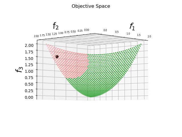
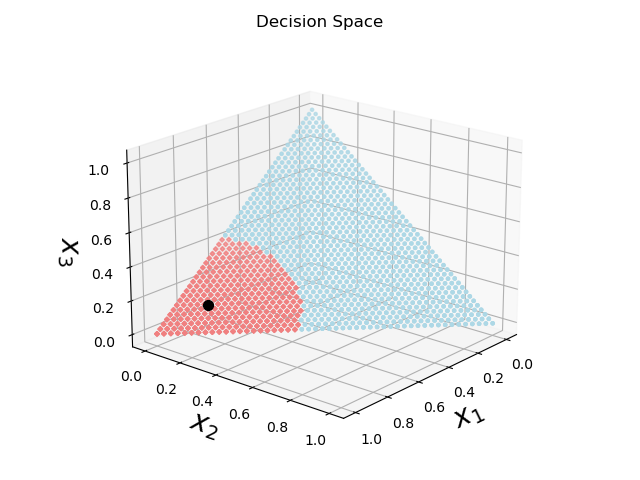
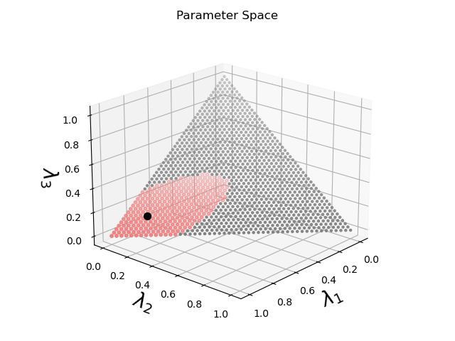
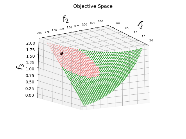
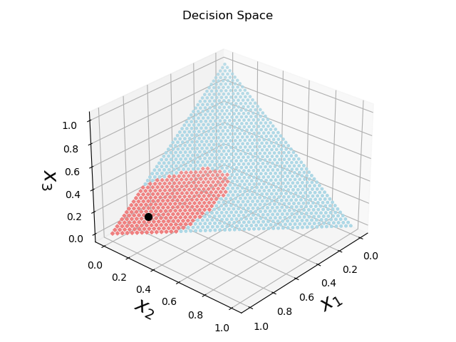
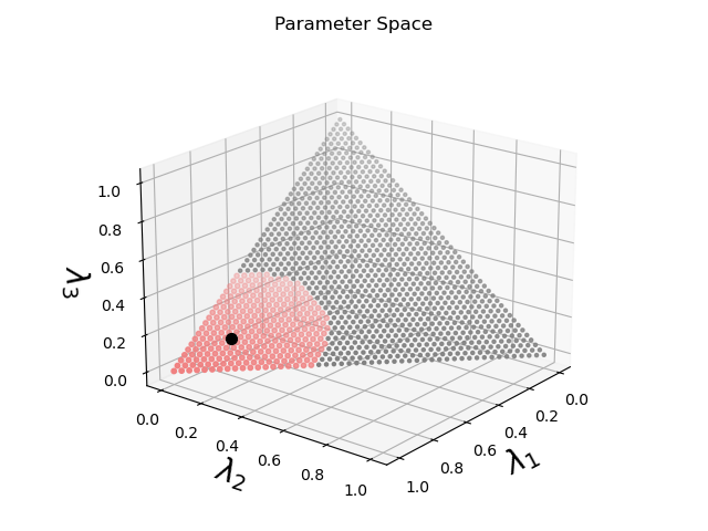
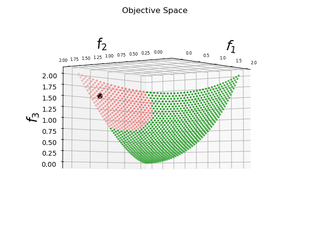
Figure 1: Pareto neighborhoods for problem ZLT1 in the parameter, objective, and decision spaces. The upper, middle, and lower plots were obtained by sampling weights from $\Lambda$ at equidistant points within $\mathcal{B}_{r}(\lambda_{c})$, $\mathcal{E}_{\alpha}(\lambda_{c})$, and $\mathcal{E}_{\beta}(\lambda_{c})$, respectively.

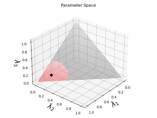
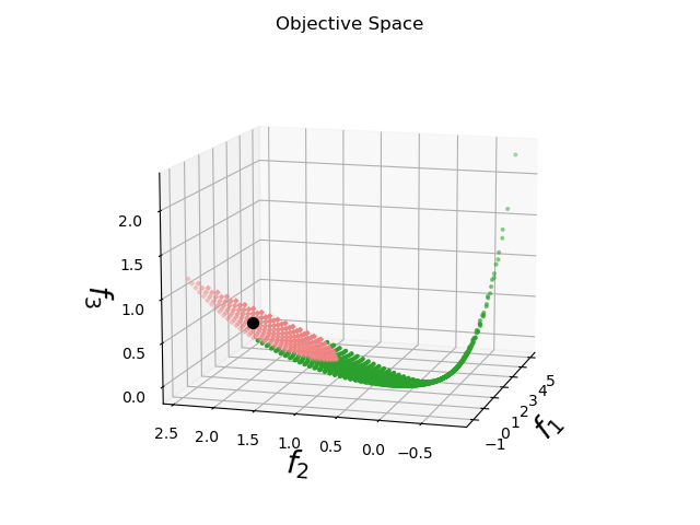
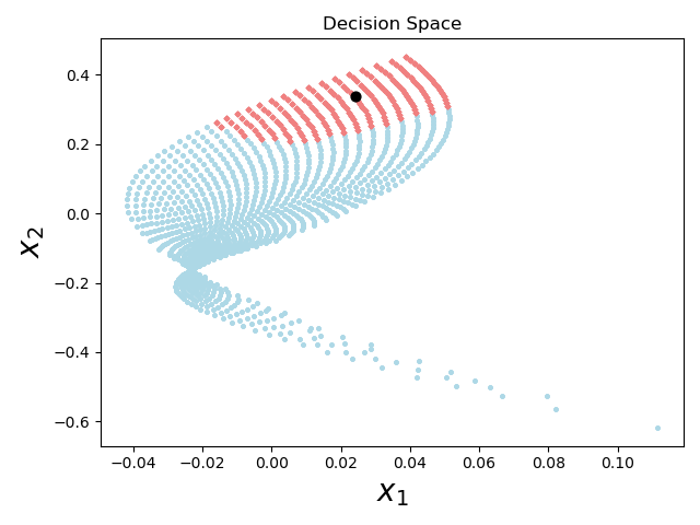
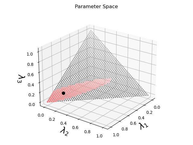
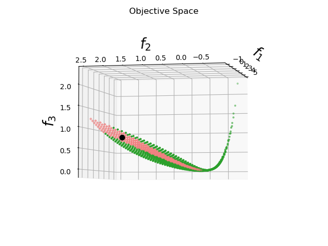
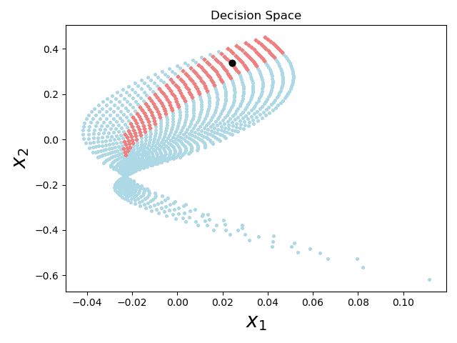
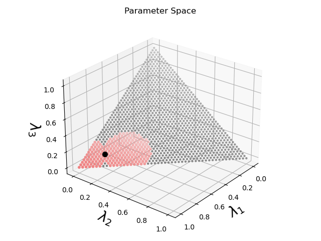
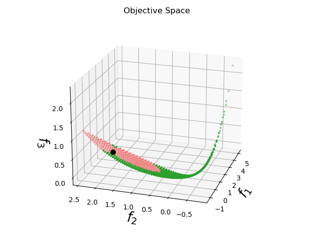
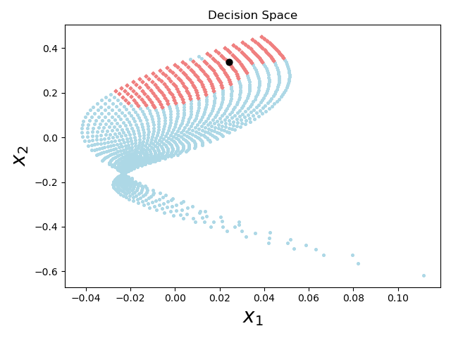
Figure 2: Pareto neighborhoods for problem GRV1 (for $\bar{n}$ in Table 2 equal to 2) in the parameter, objective, and decision spaces. The upper, middle, and lower plots were obtained by sampling weights from $\Lambda$ at equidistant points within $\mathcal{B}_{r}(\lambda_{c})$, $\mathcal{E}_{\alpha}(\lambda_{c})$, and $\mathcal{E}_{\beta}(\lambda_{c})$, respectively.

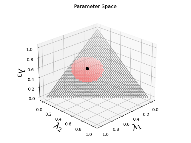
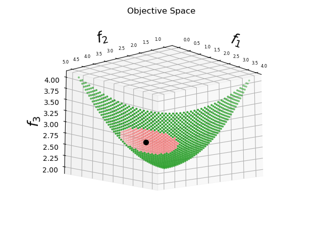
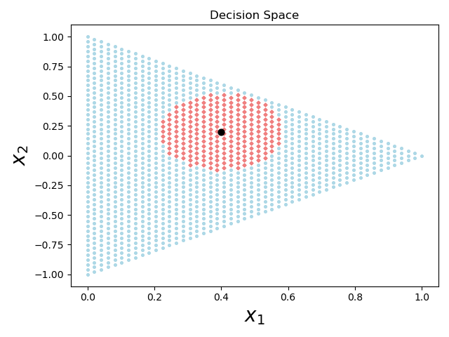
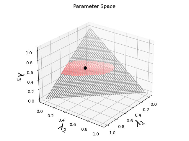
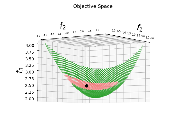
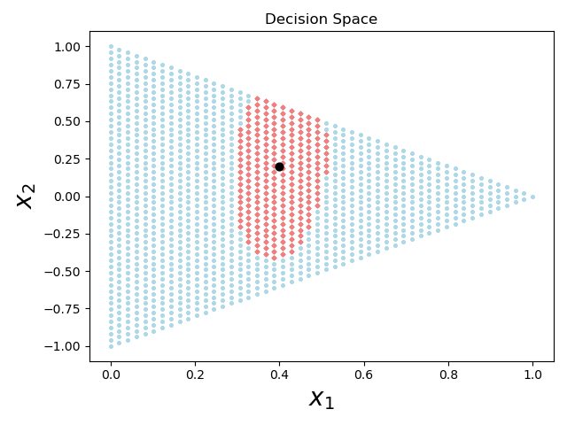
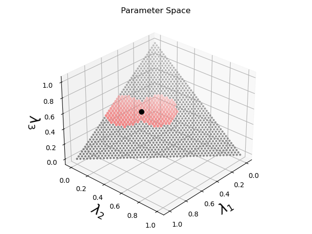
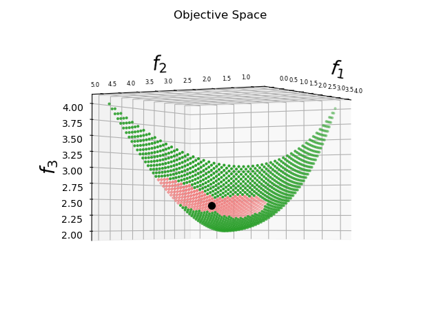
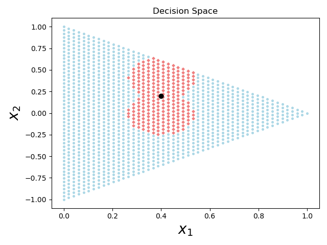
Figure 3: Pareto neighborhoods for problem VFM1 in the parameter, objective, and decision spaces. The upper, middle, and lower plots were obtained by sampling weights from $\Lambda$ at equidistant points within $\mathcal{B}_{r}(\lambda_{c})$, $\mathcal{E}_{\alpha}(\lambda_{c})$, and $\mathcal{E}_{\beta}(\lambda_{c})$, respectively.

Remark 3.1

If one wants to determine a most-changing Pareto sub-front around multiple Pareto solutions, there are several approaches one can use based on the above procedure for a single point. A first approach consists of computing a most-changing neighborhood using the centroid of the weight vectors that correspond to the given Pareto solutions. A second approach involves determining the centroid of the given Pareto solutions and computing a most-changing neighborhood using a matrix that could be either the Jacobian at the centroid or a linear combination of the Jacobians at the given Pareto solutions. A third approach consists of computing a most-changing neighborhood for all the given Pareto solutions, and then taking the union of such neighborhoods.

4 Finding knee solutions through Pareto sensitivity

In this section, we develop a single-objective optimization formulation to determine knee solutions of a Pareto front. When $q=2$, a Pareto front can be modeled in the objective space as either the curve $f_{2}=f_{2}(f_{1})$ or the curve $f_{1}=f_{1}(f_{2})$. Let $df_{2}/df_{1}$ and $df_{1}/df_{2}$ denote the derivatives of $f_{2}$ with respect to $f_{1}$ and vice versa, and let us assume their existence. These derivatives represent the slope of the tangent line to the corresponding curve at a given point. As proposed in [15, Section 6], knee solutions according to their verbal definition (trade-off between improvement and deterioration in the objectives) correspond to Pareto minimizers where these derivatives are equal in size. We then observe that a knee solution for $q=2$ minimizes $\max\{\left|df_{2}/df_{1}\right|,\left|df_{1}/df_{2}\right|\}$. When $q>2$, such an approach can be extended by minimizing the maximum derivative $\left|df_{i}/df_{j}\right|$ for all pairs $\{i,j\}\subseteq\{1,\ldots,q\}$, with $i\neq j$, in an attempt to levelize all the derivative sizes. However, such an approach is limited in practice to the fact that it would require the calculation of the entire Pareto front followed by the calculation of a model of the curves $f_{i}(f_{j})$ to compute the derivatives $\left|df_{i}/df_{j}\right|$.

To replicate the role of $|df_{i}/df_{j}|$, our approach uses the ratio between the norms of $\nabla\bar{f}_{i}(\lambda)$ and $\nabla\bar{f}_{j}(\lambda)$ (which are the columns of matrix $\nabla\bar{F}(\lambda)$ in (2.5)), resulting in the maximal-change function (MCF), which we minimize as follows

$$\min_{\lambda\in\Lambda}\ \operatorname{MCF}(\lambda),\ \text{ where }\operatorname{MCF}(\lambda)\;=\;\max_{\begin{subarray}{c}\{i,j\}\subseteq\{1,\ldots,q\}\\ i\neq j\end{subarray}}\;\frac{\lVert\nabla\bar{f}_{i}(\lambda)\rVert}{\lVert\nabla\bar{f}_{j}(\lambda)\rVert}.$$ (4.1)

Intuitively, the minimization problem in (4.1) aims to make the norms of $\nabla\bar{f}_{i}(\lambda)$ and $\nabla\bar{f}_{j}(\lambda)$ as close as possible. Recalling that derivatives measure the rate of change of a function, our snee approach defines a knee solution as a Pareto solution where the least maximal change of the Pareto front occurs. When selecting such a knee solution, the decision maker is thus protected against large trade-offs in a certain optimal way. In our numerical experiments, to avoid division by zero, we replaced $\lVert\nabla\bar{f}_{j}(\lambda)\rVert$ by $\max\{\lVert\nabla\bar{f}_{j}(\lambda)\rVert,\text{eps}\}$, where eps represents the machine precision. Once an optimal solution $\lambda_{*}$ to the minimization problem in (4.1) is obtained, one can determine a Pareto neighborhood with $\lambda_{c}=\lambda_{*}$, as described in Section 3.

Note that problem (4.1) involves the minimization of a non-smooth and nonconvex function for which subgradients involve third-order derivatives. However, the dimension of the problem is equal to the number $q$ of objective functions, typically very low, and so problem (4.1) can be efficiently solved by a derivative-free optimization (DFO) algorithm [9, 1, 31, 10].

To solve the minimization problem in (4.1), we considered two popular DFO algorithms: Nelder-Mead [36] ad DIRECT [28]. The Nelder-Mead (NM) algorithm uses a simplex of points to navigate the search space, adjusting the simplex through operations such as reflection, expansion, contraction, and shrinkage. It requires an initial starting point, but it typically involves fewer function evaluations than global methods like DIRECT, making it suitable for problems where computational efficiency is a priority. The DIRECT algorithm is a global optimization method that systematically divides the search space into hyper-rectangles, calculating objective function values to find potential global minima without requiring derivative information. It does not require an initial starting point and it may necessitate a substantial number of function evaluations. For the numerical experiments, we used the implementations of both algorithms available in the Python SciPy library [42], with default parameters. At each iteration of both algorithms, feasibility is ensured by computing orthogonal projections onto $\Lambda$.

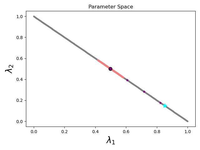
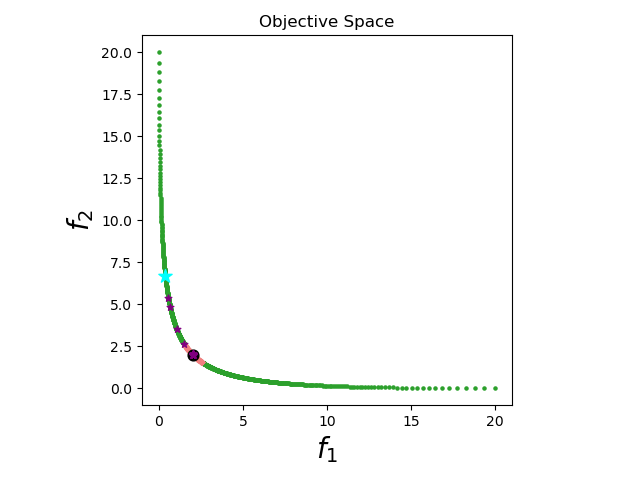
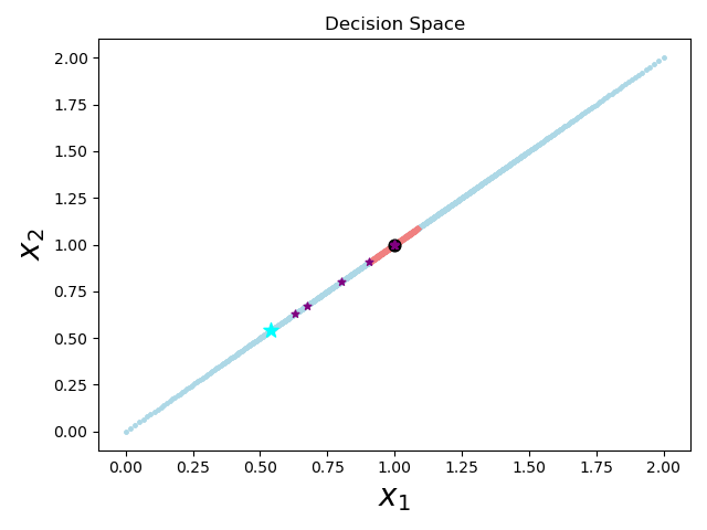
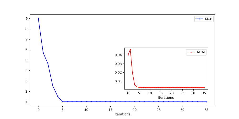
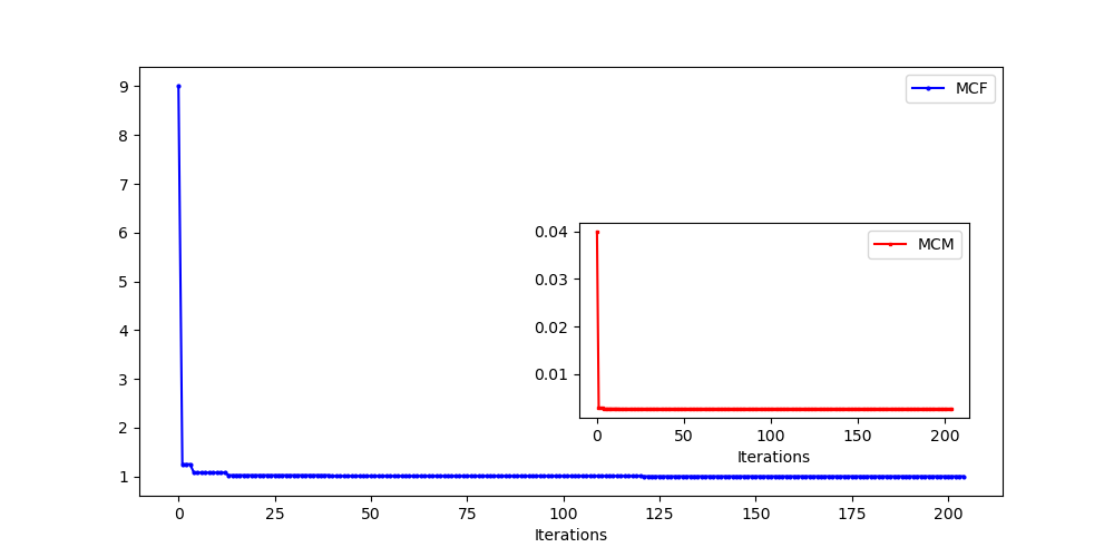
Figure 4: Knee solution for problem GRV2 (for $\bar{n}$ in Table 2 equal to 2). The upper plots show the parameter, objective, and decision spaces when applying the NM algorithm. The lower plots show the values of the $\operatorname{MCF}$ and MCM over the iterations (left: NM, right: DIRECT).

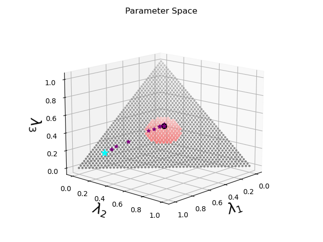
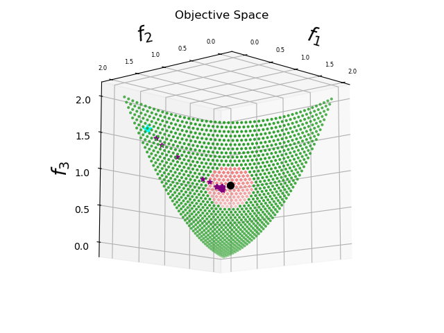
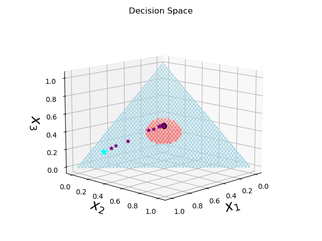
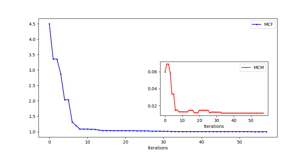
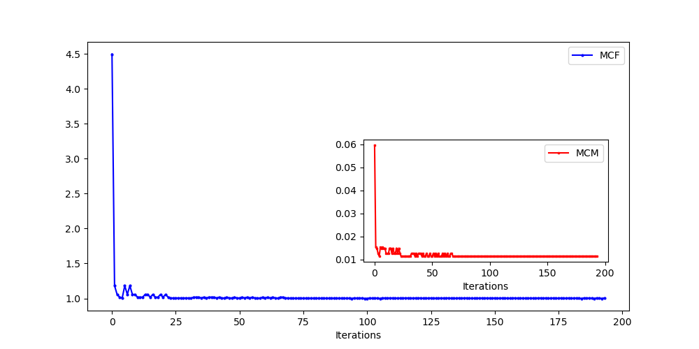
Figure 5: Knee solution for problem ZLT1. The upper plots show the parameter, objective, and decision spaces when applying the NM algorithm. The lower plots show the values of the $\operatorname{MCF}$ and MCM over the iterations (left: NM, right: DIRECT).

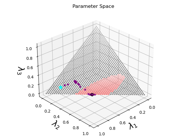
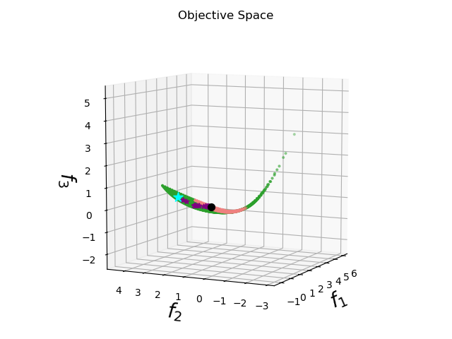
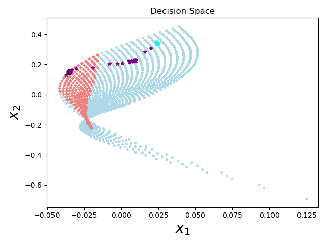
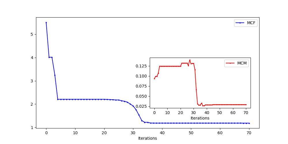
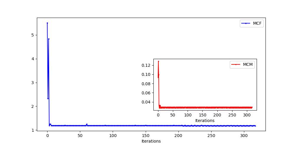
Figure 6: Knee solution for problem GRV1 (for $\bar{n}$ in Table 2 equal to 2). The upper plots show the parameter, objective, and decision spaces when applying the NM algorithm. The lower plots show the values of the $\operatorname{MCF}$ and MCM over the iterations (left: NM, right: DIRECT).

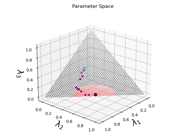
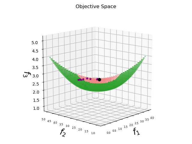
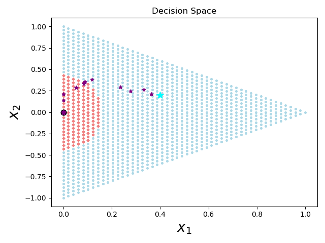
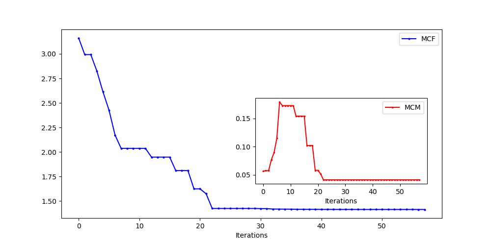
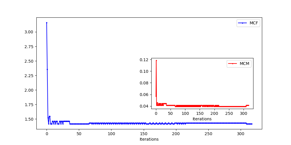
Figure 7: Knee solution for problem VFM1. The upper plots show the parameter, objective, and decision spaces when applying the NM algorithm. The lower plots show the values of the $\operatorname{MCF}$ and MCM over the iterations (left: NM, right: DIRECT).

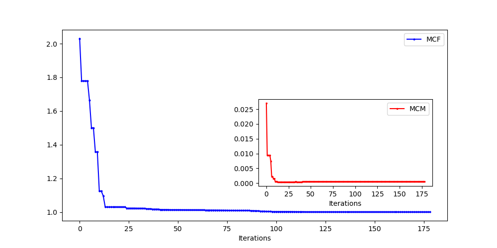
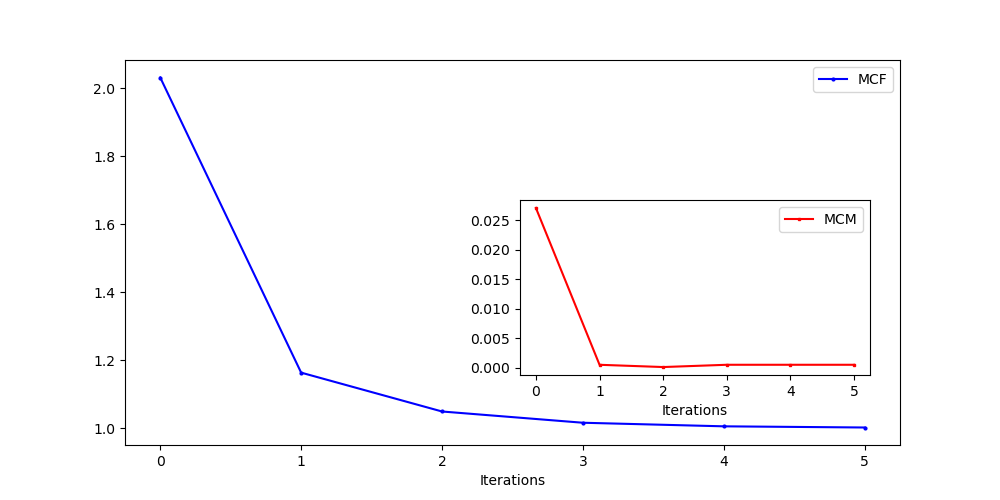
Figure 8: Knee solution for problem ZLT1$q$ (for $\bar{n}$ in Table 2 equal to 5). The plots show the values of the $\operatorname{MCF}$ and MCM over the iterations (left: NM, right: DIRECT).

We again considered the unconstrained problems from Table 2 in Appendix A. Figure 4 presents the results for problem GRV2, while Figures 5–8 present the results for problems ZLT1, GRV1, VFM1, and ZLT1$q$. For the NM algorithm, we used the weight vectors $\lambda_{c}$ from Section 3 as starting points for problems ZLT1, GRV1, VFM1, and ZLT1$q$. For problem GRV2, the starting point was arbitrarily set to $(0.9,0.1)$. In each figure, the iterates of the optimization process corresponding to the NM algorithm are represented by purple diamonds, while the starting points are indicated by cyan stars. The neighborhoods shown in the figures are the ellipsoidal ones, centered at the best point returned by the algorithm. To avoid redundancy, we do not represent the parameter, objective, and decision spaces for the DIRECT algorithm because its final solution to the minimization problem in (4.1) is nearly identical to that of the NM algorithm (there are no noticeable differences in the plots). Each figure includes plots that show the values of the $\operatorname{MCF}$ and MCM over the iterations, demonstrating their approximate correlation (the plot on the left corresponds to NM, while the plot on the right corresponds to DIRECT). One can observe that the NM and DIRECT algorithms achieve the same minimum values for the $\operatorname{MCF}$ and MCM. Note that the neighborhoods are required only for computing the MCM and not for the $\operatorname{MCF}$. To determine $x(\lambda)$ for a given $\lambda$, we used the weighted-sum method and minimized the resulting weighted-sum function by applying the BFGS algorithm, as in Section 3.

Remark 4.1

Given the approximate correlation between the $\operatorname{MCF}$ and MCM, one might think that knee solutions could be obtained by minimizing the MCM over $\lambda_{c}$ instead of the $\operatorname{MCF}$ over $\lambda$. However, such an approach presents challenges because $\operatorname{MCM}=\operatorname{MCM}(\mathcal{E}_{\alpha}(\lambda_{c}))$ depends on the neighborhood size $\alpha$. With fixed right-hand sides, the MCM may achieve a small value for a neighborhood $\mathcal{E}(\lambda_{c})$ with a small size (particularly in regions of the parameter space where the norm of $\nabla\bar{F}(\lambda_{c})$ is low), even if its center $\lambda_{c}$ is not a knee solution. Therefore, minimizing the $\operatorname{MCF}$ provides a more reliable approach.

Note that the knee solutions found by both the NM and DIRECT algorithms lie in the intermediate regions of the Pareto fronts, except for problem VFM1, where the knee solution lies on the upper boundary of the Pareto front (see Figure 7). This outcome aligns with the concept of edge-knee solutions proposed in [15] for problems with 2 objectives, but differs from the knee solutions found by the normal boundary intersection method [12, 11], which tends to identify solutions in the intermediate region of a Pareto front (when it is convex), depending on where the distance between a point on the front and the convex hull of the extreme points is maximized. If the front lacks a bulge (i.e., a region where a small improvement in any objective leads to a large deterioration in at least one other objective, which is the verbal definition of a knee solution), the solution found by our approach will not be in the intermediate region, as there is no clear knee solution according to the verbal definition.

5 Finding knee solutions through Pareto sensitivity in the constrained case

In this section, we extend the snee approach developed in Section 4 to handle constrained MOO problems. We start by pointing out that such an extension requires only a recalculation of the sensitivity $\nabla x(\lambda)$ under the presence of constraints, as everything else lies in the space of weights and encapsulates the details of the solution of each weighted-sum subproblem. When dealing with constrained MOO problems, instead of using the first-order necessary unconstrained optimality conditions in (2.3), we compute $\nabla x(\lambda)$ from the corresponding conditions under the presence of constraints, typically referred to as the first-order KKT conditions, in particular from the equality part of such conditions (the so-called KKT system).

Let us consider the following constrained MOO problem

$$\min_{x\in X}F(x),\ \text{ with }\ X=\{x\in\mathbb{R}^{n}~|~c_{j}(x)\leq 0,\;j\in I,\text{ and }c_{j}(x)=0,\;j\in E\},$$ (5.1)

where $I$ and $E$ are finite index sets used to denote inequality and equality constraints, respectively. Appendix B includes the derivation of $\nabla x(\lambda)$ using the first-order KKT system associated with problem (5.1). We will assume a well-known set of conditions in constrained optimization theory (LICQ, strict complementarity slackness, and second-order sufficient optimality), as detailed in Assumption B.1, in order to secure the required matrix invertibility in the derivative calculation. By applying the chain rule as we did to derive (2.5), but now using the matrix $\nabla x(\lambda)$ from (B.4) instead of (2.4), we obtain that the transpose of the Jacobian matrix of $\bar{F}$ at $\lambda$ is given by

$$\nabla\bar{F}(\lambda) =\;\nabla x(\lambda)\nabla_{x}F(x(\lambda))$$ (5.2)

$$=\;-\nabla_{\lambda}K\nabla_{w}K^{-1}L(\nabla_{x}f_{1},\ldots,\nabla_{x}f_{q}),$$

where $K$ is the vector function associated with the KKT system of problem (5.1) and $w$ is a vector formed by primal variables $x$ and Lagrange multipliers. The matrices $\nabla_{\lambda}K$ and $\nabla_{w}K$ are the Jacobians of $K$ with respect to $\lambda$ and $w$, respectively (see (B.2)), and $L=\begin{pmatrix}\mathbf{I}_{n}&\mathbf{0}\end{pmatrix}^{\top}$. In (5.2), all gradients $\nabla_{x}f_{i}$ are evaluated at $x(\lambda)$, with $i\in\{1,\ldots,q\}$, and $\nabla_{\lambda}K$ and $\nabla_{w}K$ are evaluated at $w(\lambda)$. Note that matrix $\nabla\bar{F}(\lambda)$ in (5.2) is no longer symmetric as in the unconstrained case (2.5), but this does not change anything in regards to the applicability of the snee approach.

To solve the minimization problem in (4.1), where $\nabla\bar{f}_{i}(\lambda)$ and $\nabla\bar{f}_{j}(\lambda)$ in the $\operatorname{MCF}$ now correspond to the columns of matrix $\nabla\bar{F}(\lambda)$ in (5.2) instead of (2.5), we again applied the NM and DIRECT algorithms, as in Section 4. Figures 9–11 show the results obtained by the NM algorithm for problems DAS1, DO2DK, and VFM1constr from Table 3 in Appendix A. We considered two configurations for problem DO2DK by selecting the constraint right-hand side $r$ from $\{0.5,1\}$, where $1$ corresponds to a larger feasible set and $0.5$ results in a tighter feasible set. For the NM algorithm, we arbitrarily used the weight vectors $(0.4,0.6)$, $(0.2,0.8)$, and $(0.4,0.2,0.4)$ as starting points for problems DAS1, DO2DK, and VFM1constr, respectively. To determine $x(\lambda)$ for a given $\lambda$, we used the weighted-sum method and minimized the resulting weighted-sum function by applying the SLSQP algorithm [29], which is designed for solving constrained optimization problems through sequential quadratic programming. We ran the SLSQP algorithm implementation available in the Python SciPy library [42], with default parameters. Similar to Section 4, the neighborhoods shown in the figures are the ellipsoidal ones, centered at the best point returned by the algorithm. For all the problems, using a fixed neighborhood size $\alpha$ resulted in ellipsoidal neighborhoods that either had no solutions or contained the entire simplex set at certain iterations. Therefore, we adopted the same adaptive rule used for GRV2 in Section 4. Again, the neighborhoods are required only for computing the MCM and not for the $\operatorname{MCF}$.

Figure 9 and the upper plots of Figure 10 show that the knee solutions for problems DAS1 and for problem DO2DK when $r=1$ (i.e., the feasible set is relatively large) lie in the intermediate region of the Pareto front. In contrast, in the lower plots of Figure 10 and in Figure 11, our snee approach leads to solutions that correspond to points on the boundary of the Pareto front. Similar to Section 4, the reason why we do not observe a knee solution in the intermediate region for DO2DK with $r=0.5$ and VFM1constr is due to the lack of a bulge in the Pareto front within the interior of the feasible set. Instead, the normal boundary intersection method would have returned a point in the intermediate region, regardless of the presence of a bulge.

For the DIRECT algorithm, we include in Figure 12 the plots showing the values of the $\operatorname{MCF}$ and MCM over the iterations for all constrained problems from Table 3, and we do not represent the parameter, objective, and decision spaces because the final solution to the minimization problem in (4.1) is nearly identical to that of the NM algorithm, except for problem VFM1constr. For VFM1constr, the final solution found by DIRECT lies on the west boundary of the Pareto front (see objective space of Figure 13), whereas the solution found by NM lies on the upper boundary, as shown in the objective space of Figure 11. Such differences arise because the $\operatorname{MCF}$ is non-convex, causing the NM algorithm to get stuck in local minimizers, while the DIRECT algorithm finds global minimizers (or, at least, better local minimizers than NM). It becomes then evident that knee solutions can have a local or global nature. Interestingly, the results for problem VFM1constr shown in plot d) of Figure 12 suggest that a minimizer of the $\operatorname{MCF}$ may not correspond to a minimizer of the $\operatorname{MCM}$. This discrepancy arises because the ellipsoidal neighborhood becomes degenerate at the point corresponding to the optimal solution (and nearby points), as shown in the objective space in Figure 13. The degeneracy occurs because the matrix $\nabla\bar{F}(\lambda)$ is highly ill-conditioned, with two of its three eigenvalues close to zero, resulting in an elongated ellipsoid that inflates the value of the $\operatorname{MCM}$. This observation confirms that minimizing the $\operatorname{MCM}$ instead of the $\operatorname{MCF}$ is not a reliable approach for finding knee solutions, as previously noted in Remark 4.1.

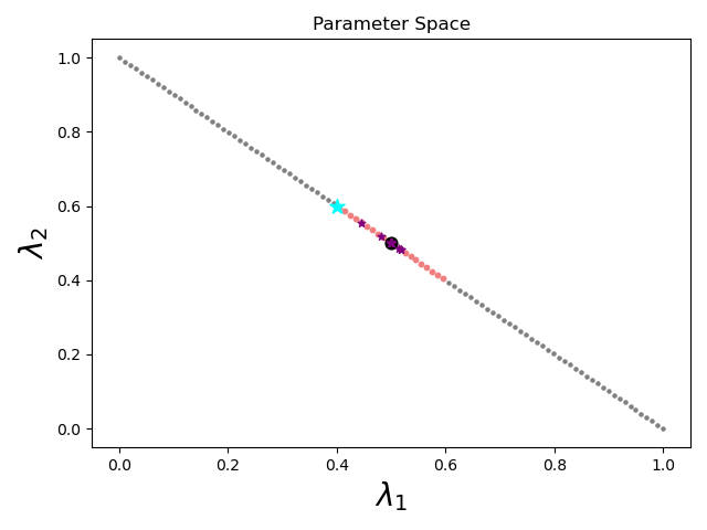
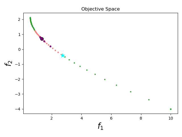
Figure 9: Knee solution for problem DAS1 when applying the NM algorithm. The left two plots show the parameter and objective spaces. The right plot shows the values of the $\operatorname{MCF}$ and MCM over the iterations.

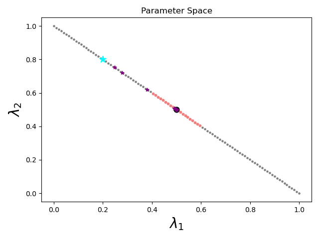
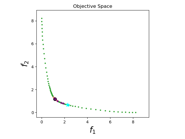
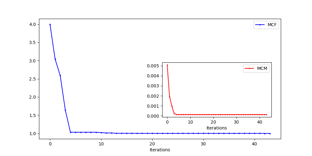
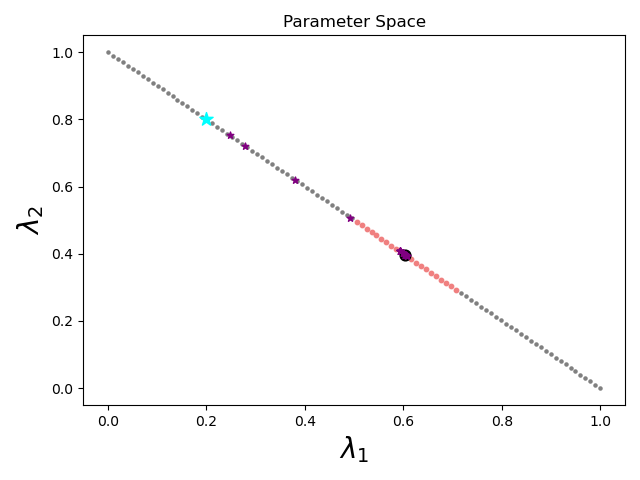
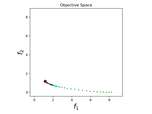
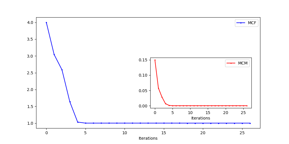
Figure 10: Knee solutions for problem DO2DK (upper plots: $r=1$, lower plots: $r=0.5$) when applying the NM algorithm. The figure includes plots of the parameter and objective spaces, as well as the values of the $\operatorname{MCF}$ and MCM over the iterations.

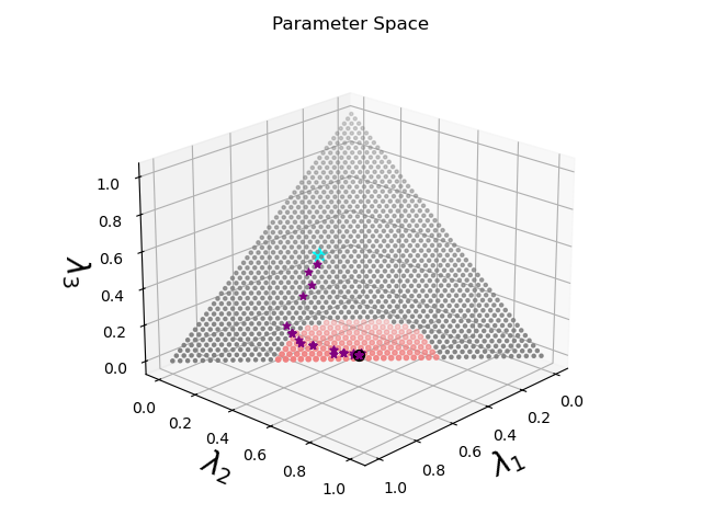
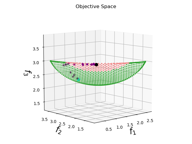
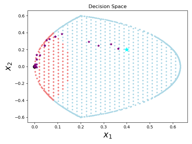
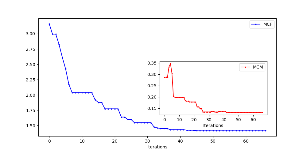
Figure 11: Knee solution for problem VFM1constr when applying the NM algorithm. The figure includes plots of the parameter, objective, and decision spaces, as well as the values of the $\operatorname{MCF}$ and MCM over the iterations.

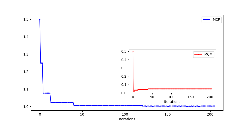
(a) DAS1

(b) DO2DK (for $r$ in Table 3 equal to 1)

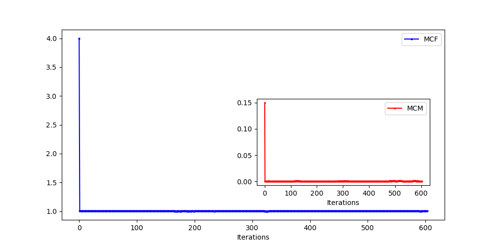
(c) DO2DK (for $r$ in Table 3 equal to 0.5)

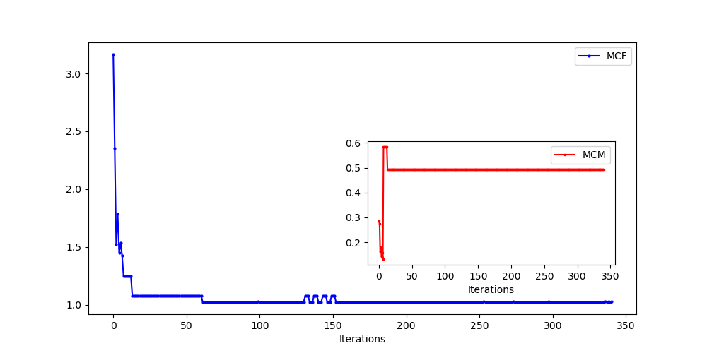
(d) VFM1constr

Figure 12: Plots that show the values of the $\operatorname{MCF}$ and MCM over the iterations when applying the DIRECT algorithm to determine knee solutions for constrained problems.

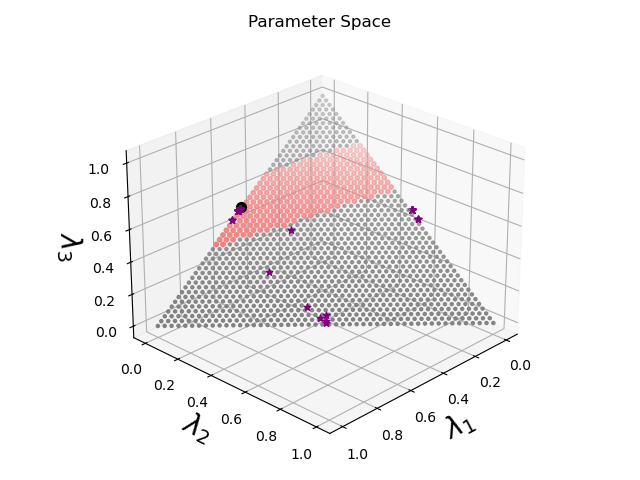
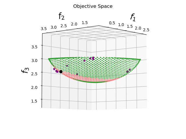
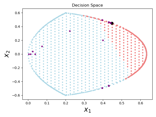
Figure 13: Knee solution for problem VFM1constr. The plots show the parameter, objective, and decision spaces when applying the DIRECT algorithm.

6 Concluding remarks and future work

In this paper, we have seen how to use first-order rates of variation of Pareto solutions to better understand the tradeoffs of a Pareto front in multi-objective optimization. We have used such sensitivity rates to provide an answer to the open question of how to rigorously compute knee solutions, i.e., points where a small improvement in any objective leads to a large deterioration in at least one other objective. Based on the observation that such solutions lie where slopes in a Pareto front are levelized, we introduced a problem formulation (4.1) capable of accurately identifying the desired knee solutions. The corner stone of our approach is the ability to compute the gradient $\nabla f_{i}(x(\lambda))$ of each individual objective function $f_{i}$ through the rate of variation $\nabla x(\lambda)$ of the Pareto solution $x(\lambda)$, where $\lambda$ denotes a vector of objective weights. The formulation (4.1) was used to compute knee solutions following their verbal definition regardless of the presence of constraints. We called our approach snee to emphasize the use of Pareto sensitivity in the calculation of the derivatives of $F(x(\lambda))$. We have also shown in this paper how to compute the most-changing Pareto sub-fronts around a Pareto solution. Such sub-fronts are obtained from neighborhoods constructed in the decision space using the pseudo-inverse of the Jacobian matrix of the vector function $F(x(\lambda))$ and include points that are distributed along directions of maximum change.

The techniques used in our approach are still restricted to scalarized methods. In the current paper, we explored the weighted-sum method, which requires convexity of the objective functions in $F$ for a complete coverage of the Pareto front. Our approach can be extended to the $\varepsilon$-constrained method, which converts a multi-objective problem into a single-objective constrained problem where one objective is optimized subject to constraints requiring the other objectives to be below varying thresholds. Given a positive threshold $\varepsilon$ and denoting the corresponding Pareto solution as $x(\varepsilon)$, one can consider a neighborhood of $\varepsilon$ to determine a Pareto neighborhood around $x(\varepsilon)$. To compute knee solutions using our snee approach, one can consider a reformulation of problem (4.1) in terms of $\varepsilon$. Although the $\varepsilon$-constrained method does not explicitly require convexity for a complete coverage of the Pareto front, it requires a global solution of a constrained optimization problem. Therefore, our future work will focus on exploring techniques that do not rely on scalarized methods.

Appendix A MOO test problems

Table 2 specifies the unconstrained test problems considered in the experiments for Sections 3 and 4, along with the number of variables and objectives (i.e., $n$ and $q$, respectively). All of the problems have strictly convex objective functions, which is in accordance with Assumption 2.1 in Section 2.

Problem	$n$	$q$	Ref.	Objective Functions
ZLT1	3	3	[27]	$f_{1}(x_{1},x_{2},x_{3})=(x_{1}-1)^{2}+x_{2}^{2}+x_{3}^{2}$
				$f_{2}(x_{1},x_{2},x_{3})=x_{1}^{2}+(x_{2}-1)^{2}+x_{3}^{2}$
				$f_{3}(x_{1},x_{2},x_{3})=x_{1}^{2}+x_{2}^{2}+(x_{3}-1)^{2}$
GRV1	$2\bar{n}$	3		$f_{1}(x_{1},x_{2})=\frac{1}{2}x_{1}^{\top}H_{1}x_{1}+\frac{1}{2}x_{2}^{\top}H_{2}x_{2}+x_{1}^{\top}H_{3}x_{2}+a_{1}^{\top}x_{1}+a_{2}^{\top}x_{2}$
				$f_{2}(x_{1},x_{2})=\frac{1}{2}x_{1}^{\top}H_{3}x_{1}+\frac{1}{2}x_{2}^{\top}H_{4}x_{2}+x_{1}^{\top}H_{5}x_{2}+a_{3}^{\top}x_{1}+a_{4}^{\top}x_{2}$
				$f_{3}(x_{1},x_{2})=\frac{1}{2}x_{1}^{\top}H_{7}x_{1}+\frac{1}{2}x_{2}^{\top}H_{8}x_{2}+x_{1}^{\top}H_{9}x_{2}+a_{5}^{\top}x_{1}+a_{6}^{\top}x_{2}$
VFM1	$2$	3	[27]	$f_{1}(x_{1},x_{2})=x_{1}^{2}+(x_{2}-1)^{2}$
				$f_{2}(x_{1},x_{2})=x_{1}^{2}+(x_{2}+1)^{2}+1$
				$f_{3}(x_{1},x_{2})=(x_{1}-1)^{2}+x_{2}^{2}+2$
ZLT1$q$	$\bar{n}$	$\bar{q}$	[27]	$f_{j}(x)=(x_{j}-1)^{2}+\sum_{1\leq i\leq\bar{n},i\neq j}x_{i}^{2},\quad j\in\{1,\ldots,\bar{q}\}$
GRV2	$\bar{n}$	$2$		$f_{1}(x)=\frac{1}{\bar{n}}\sum_{i=1}^{\bar{n}}x_{i}^{2}+\frac{1}{2}\sum_{i=1}^{\bar{n}}x_{i}^{4}$
				$f_{2}(x)=\frac{1}{\bar{n}}\sum_{i=1}^{\bar{n}}(x_{i}-2)^{2}+\frac{1}{2}\sum_{i=1}^{\bar{n}}(x_{i}-2)^{4}$

Table 2: Unconstrained test problems ($\bar{n}$ and $\bar{q}$ are arbitrary positive scalars).

In Problem GRV1, $a_{1}$, $a_{2}$, and $a_{5}$ were randomly generated according to a uniform distribution over $[-5,0)$, resulting in $a_{1}=-1.87$, $a_{2}=-4.75$, and $a_{5}=-0.78$. Similarly, $a_{3}$, $a_{4}$, and $a_{6}$ were randomly generated according to a uniform distribution over $[0,5)$, resulting in $a_{3}=3.66$, $a_{4}=2.99$, and $a_{6}=0.78$. Additionally, we randomly generated three $\bar{n}\times\bar{n}$ symmetric positive definite matrices $H^{(1)}$, $H^{(2)}$, and $H^{(3)}$, and we set the matrices in the objective functions $f_{i}$, with $i\in\{1,2,3\}$, as follows:

$$H^{(1)}=\begin{bmatrix}H_{1}&H_{3}\\ H_{3}^{\top}&H_{2}\end{bmatrix}=\begin{bmatrix}50.82&-0.23\\ -0.23&10.57\end{bmatrix},\quad H^{(2)}=\begin{bmatrix}H_{4}&H_{6}\\ H_{6}^{\top}&H_{5}\end{bmatrix}=\begin{bmatrix}38.25&12.19\\ 12.19&6.53\end{bmatrix},$$

$$H^{(3)}=\begin{bmatrix}H_{7}&H_{9}\\ H_{9}^{\top}&H_{8}\end{bmatrix}=\begin{bmatrix}45.10&-9.55\\ -9.55&9.91\end{bmatrix}.$$

Table 3 specifies the constrained test problems considered in the experiments for Section 5, along with the number of variables and objectives (i.e., $n$ and $q$, respectively). Problems DAS1 and DO2DK are well-known in the MOO literature. They have a convex Pareto front, despite some of the objective functions being non-convex.

Problem	$n$	$q$	Ref.	Objective Functions and Constraints
DAS1	$5$	$2$	[12]	$f_{1}(x_{1},\ldots,x_{5})=x_{1}^{2}+x_{2}^{2}+x_{3}^{2}+x_{4}^{2}+x_{5}^{2}$
				$f_{2}(x_{1},\ldots,x_{5})=3x_{1}+2x_{2}-x_{3}/3+0.01(x_{4}-x_{5})^{3}$
				$c_{1}(x_{1},\ldots,x_{5})=x_{1}^{2}+x_{2}^{2}+x_{3}^{2}+x_{4}^{2}+x_{5}^{2}-10\leq 0$
				$c_{2}(x_{1},\ldots,x_{5})=x_{1}+2x_{2}-x_{3}-0.5x_{4}+x_{5}-2=0$
				$c_{3}(x_{1},\ldots,x_{5})=4x_{1}-2x_{2}+0.8x_{3}+0.6x_{4}+0.5x_{5}^{2}=0$
DO2DK	$30$	$2$	[5, 16, 13]	$f_{1}(x)=g_{1}(x)g_{2}(x_{1})\left(\sin\left(\pi x_{1}/2+\pi\right)+1\right)$
				$f_{2}(x)=g_{1}(x)g_{2}(x_{1})\left(\cos\left(\pi x_{1}/2+\pi\right)+1\right)$
				$g_{1}(x)=1+\frac{9}{n-1}\sum_{i=2}^{n}x_{i}$
				$g_{2}(x_{1})=5+10\left(x_{1}-0.5\right)^{2}+\cos\left(2\pi x_{1}\right)\cdot 2^{\frac{1}{2}}$
				$c_{j}(x)=-x_{j}\leq 0,\quad j\in\{1,2,\ldots,n\}$
				$c_{n+j}(x)=x_{j}-r\leq 0,\quad j\in\{1,2,\ldots,n\}$
VFM1constr	$2$	$3$		$f_{1}(x_{1},x_{2})=x_{1}^{2}+(x_{2}-1)^{2}$
				$f_{2}(x_{1},x_{2})=x_{1}^{2}+(x_{2}+1)^{2}+1$
				$f_{3}(x_{1},x_{2})=(x_{1}-1)^{2}+x_{2}^{2}+2$
				$c_{1}(x_{1},x_{2})=x_{1}^{2}+x_{2}^{2}-0.8\leq 0$
				$c_{2}(x_{1},x_{2})=(x_{1}-1)^{2}+x_{2}^{2}-1\leq 0$

Table 3: Constrained test problems ($r$ in DO2DK is an arbitrary positive scalar

that we use to tighten the feasible set).

Appendix B Calculating $\nabla x(\lambda)$ in the constrained case

Recall problem (5.1) in Section 5. Denoting $c_{I}(x)=(c_{j}(x),\,j\in I)$ and $c_{E}(x)=(c_{j}(x),\,j\in E)$, and given $\lambda\in\Lambda$, the Lagrangian function of problem (5.1) is defined as $\mathcal{L}(x,z_{I},z_{E})=\sum_{i=1}^{q}\lambda_{i}f_{i}(x)+c_{I}(x)^{\top}z_{I}+c_{E}(x)^{\top}z_{E}$, where $z_{I}$ and $z_{E}$ are vectors of Lagrange multipliers. We assume in Assumption B.1 below that the constraint functions are twice continuously differentiable and there exists a solution $x(\lambda)$ satisfying the KKT conditions for problem (5.1) with associated vectors of multipliers $(z_{I}(\lambda),z_{E}(\lambda))$. Specifically, the first-order KKT system for problem (5.1) at $x(\lambda)$ is given by (see [34, Theorem 3.1.5])

$$\begin{cases}\sum_{i=1}^{q}\lambda_{i}\nabla_{x}f_{i}(x(\lambda))+\nabla_{x}c_{I}(x(\lambda))\,z_{I}(\lambda)+\nabla_{x}c_{E}(x(\lambda))\,z_{E}(\lambda)=0,\\ z_{I}(\lambda)\circ c_{I}(x(\lambda))=0,\\ c_{E}(x(\lambda))=0,\end{cases}$$ (B.1)

where $\circ$ denotes the element-wise multiplication of two vectors. We do not include the non-negativity of the multipliers in $z_{I}(\lambda)$ and the satisfaction of the inequality constraints in (B.1) because they are not necessary for the derivation below. In Assumption B.1 below, we also require the linear independence constraint qualification (LICQ), strict complementarity slackness (SCS), and the second-order sufficient condition (SOSC), and we refer to [37, Chapter 12] for their definitions.

Assumption B.1 (Existence of Pareto minimizer (LL constrained case))

.Let $X$ be defined as in problem (5.1). The constraint functions $c_{j}$, with $j\in I\cup E$, are twice continuously differentiable. There exists a solution $x(\lambda)$ satisfying the KKT conditions with associated multipliers $(z_{I}(\lambda),z_{E}(\lambda))$ such that the LICQ, SCS, and SOSC are satisfied.

Under Assumption B.1, based on [21, 19, 20, 33], the vectors of multipliers $z_{I}(\lambda)$ and $z_{E}(\lambda)$ associated with $x(\lambda)$ are unique, and the vector function $w(\lambda)=(x(\lambda),z_{I}(\lambda),z_{E}(\lambda))^{\top}$ is once continuously differentiable for any given $\lambda$. Let us now introduce a vector function $K$ such that the KKT system (B.1) can be written as $K(w(\lambda))=0$. Applying the chain rule to such an equation, we obtain $\nabla_{w}K^{\top}\nabla w^{\top}=-\nabla_{\lambda}K^{\top}$, with

$$\nabla_{\lambda}K^{\top}=\begin{pmatrix}\nabla_{x\lambda}^{2}\mathcal{L}\\ 0\\ 0\end{pmatrix}\;\text{ and }\;\nabla_{w}K^{\top}=\begin{pmatrix}\nabla_{xx}^{2}\mathcal{L}&&\nabla_{x}c_{I}&&\nabla_{x}c_{E}\\ z_{I}\circ\nabla_{x}c_{I}^{\top}&&C_{I}&&0\\ \nabla_{x}c_{E}^{\top}&&0&&0\end{pmatrix},$$ (B.2)

where $\nabla_{x\lambda}\mathcal{L}$ and $\nabla_{xx}\mathcal{L}$ are evaluated at $w(\lambda)$, the Jacobian matrices $\nabla_{x}c_{I}^{\top}$ and $\nabla_{x}c_{E}^{\top}$ are evaluated at $x(\lambda)$, $C_{I}$ is a diagonal matrix with elements defined by $c_{I}(x(\lambda))$, and $z_{I}\circ\nabla_{\lambda}c_{I}^{\top}$ represents a matrix formed by element-wise multiplication of the entries of $z_{I}$ with the corresponding rows of $\nabla_{x}c_{I}^{\top}$.

Under Assumption B.1, it is well known that the Jacobian $\nabla_{w}K^{\top}$ is non-singular at $w(\lambda)$ (see [33, 37]). Therefore, we have

$$\nabla w\;=\;\begin{pmatrix}\nabla x,\nabla z_{I},\nabla z_{E}\end{pmatrix}\;=\;-\nabla_{\lambda}K\,\nabla_{w}K^{-1}.$$ (B.3)

Following [26, Subsection 2.2], we can now introduce a matrix $L=\begin{pmatrix}\mathbf{I}_{n}&\mathbf{0}\end{pmatrix}^{\top}$ to extract the columns of (B.3) that correspond to the $\nabla x(\lambda)$ term, where $\mathbf{I}_{n}$ denotes an identity matrix of size $n$ and $\mathbf{0}$ represents a null matrix of dimensions $n\times\big{(}|I|+|E|\big{)}$, resulting in

$$\nabla x(\lambda)\;=\;-\nabla_{\lambda}K\nabla_{w}K^{-1}L.$$ (B.4)

References

- Audet and Hare [2017] C. Audet and W. Hare. Derivative-Free and Blackbox Optimization. Springer Series in Operations Research and Financial Engineering. Springer, Cham, 2017. With a foreword by John E. Dennis Jr.
- Audet et al. [2021] C. Audet, J. Bigeon, D. Cartier, S. Le Digabel, and L. Salomon. Performance indicators in multiobjective optimization. European Journal of Operational Research, 292:397–422, 2021.
- Bechikh et al. [2010] S. Bechikh, L. Ben Said, and K. Ghédira. Searching for knee regions in multi-objective optimization using mobile reference points. In Proceedings of the 2010 ACM Symposium on Applied Computing, SAC ’10, page 1118–1125, New York, NY, USA, 2010. Association for Computing Machinery.
- Boresta et al. [2024] M. Boresta, T. Giovannelli, and M. Roma. Managing low–acuity patients in an emergency department through simulation–based multiobjective optimization using a neural network metamodel. Health Care Management Science, pages 1–21, 2024.
- Branke et al. [2004] J. Branke, K. Deb, H. Dierolf, and M. Osswald. Finding knees in multi-objective optimization. In Parallel Problem Solving from Nature - PPSN VIII, pages 722–731, Berlin, Heidelberg, 2004. Springer Berlin Heidelberg.
- Burke et al. [1988] W.J. Burke, H.M. Merrill, F.C. Schweppe, B.E. Lovell, M.F. McCoy, and S.A. Monohon. Trade off methods in system planning. IEEE Transactions on Power Systems, 3:1284–1290, 1988. doi: 10.1109/59.14593.
- Chen et al. [2023] L. Chen, H. Fernando, Y. Ying, and T. Chen. Three-Way Trade-Off in Multi-Objective Learning: Optimization, Generalization and Conflict-Avoidance. arXiv e-prints, art. arXiv:2305.20057, May 2023.
- Chiandussi et al. [2012] G. Chiandussi, M. Codegone, S. Ferrero, and F.E. Varesio. Comparison of multi-objective optimization methodologies for engineering applications. Computers & Mathematics with Applications, 63:912–942, 2012.
- Conn et al. [2009] A. R. Conn, K. Scheinberg, and L. N. Vicente. Introduction to Derivative-Free Optimization. MPS/SIAM Book Series on Optimization, SIAM, Philadelphia, USA, 2009.
- Custódio et al. [2017] A. L. Custódio, K. Scheinberg, and L. N. Vicente. Chapter 37: Methodologies and software for derivative-free optimization. In Advances and Trends in Optimization with Engineering Applications, pages 495–506. SIAM, 2017.
- Das [1999] I. Das. On characterizing the “knee” of the pareto curve based on normal-boundary intersection. Structural Optimization, 18:107–115, 1999.
- Das and Dennis [1998] I. Das and J. E. Dennis. Normal-boundary intersection: A new method for generating the Pareto surface in nonlinear multicriteria optimization problems. SIAM Journal on Optimization, 8:631–657, 1998.
- Deb [1999] K. Deb. Multi-objective genetic algorithms: Problem difficulties and construction of test problems. Evolutionary Computation, 7:205–230, 1999.
- Deb [2003] K. Deb. Multi-objective evolutionary algorithms: introducing bias among Pareto-optimal solutions, page 263–292. Springer-Verlag, Berlin, Heidelberg, 2003.
- Deb and Gupta [2010] K. Deb and S. Gupta. Understanding knee points in bicriteria problems and their implications as preferred solution principles. Engineering Optimization, 43, 08 2010.
- Deb et al. [2002] K. Deb, L. Thiele, M. Laumanns, and E. Zitzler. Scalable multi-objective optimization test problems. In Proceedings of the 2002 Congress on Evolutionary Computation. CEC’02 (Cat. No.02TH8600), volume 1, pages 825–830 vol.1, 2002.
- Demir et al. [2014] E. Demir, T. Bektaş, and G. Laporte. The bi-objective pollution-routing problem. European Journal of Operational Research, 232:464–478, 2014.
- Ehrgott [2005] M. Ehrgott. Multicriteria Optimization, volume 491. Springer Science & Business Media, Berlin, 2005.
- Fiacco [1976] A. V. Fiacco. Sensitivity analysis for nonlinear programming using penalty methods. Mathematical Programming, 10:287–311, 1976.
- Fiacco [1983] A. V. Fiacco. Introduction to sensitivity and stability analysis in nonlinear programming, volume 165 of Mathematics in Science and Engineering. Academic Press, Inc., Orlando, FL, 1983.
- Fiacco and McCormick [1968] A. V. Fiacco and G. P. McCormick. Nonlinear programming: Sequential unconstrained minimization techniques. John Wiley & Sons, Inc., New York-London-Sydney, 1968.
- Fleming et al. [2005] P. J. Fleming, R. C. Purshouse, and R. J. Lygoe. Many-objective optimization: An engineering design perspective. In Evolutionary Multi-Criterion Optimization, pages 14–32, Berlin, Heidelberg, 2005. Springer Berlin Heidelberg.
- Fletcher [1987] R. Fletcher. Practical Methods of Optimization. Wiley, Chichester; New York, 1987.
- Geoffrion [1968] A. M. Geoffrion. Proper efficiency and the theory of vector maximization. Journal of Mathematical Analysis and Applications, 22:618–630, 1968.
- Giovannelli and Vicente [2023] T. Giovannelli and L. N. Vicente. An integrated assignment, routing, and speed model for roadway mobility and transportation with environmental, efficiency, and service goals. Transportation research part C: Emerging technologies, 152:104144, 2023.
- Giovannelli et al. [2022] T. Giovannelli, G. Kent, and L. N. Vicente. Inexact bilevel stochastic gradient methods for constrained and unconstrained lower-level problems. ISE Technical Report 21T-025, Lehigh University, December 2022.
- Huband et al. [2006] S. Huband, P. Hingston, L. Barone, and R. Lyndon While. A review of multiobjective test problems and a scalable test problem toolkit. IEEE Transactions on Evolutionary Computation, 10:477–506, 2006.
- Jones et al. [1993] D. R. Jones, C. D. Perttunen, and B. E. Stuckman. Lipschitzian optimization without the lipschitz constant. Journal of Optimization Theory and Applications, 79:157–181, 1993.
- Kraft [1988] D. Kraft. A software package for sequential quadratic programming. Technical Report DFVLR-FB 88-28, DLR German Aerospace Center — Institute for Flight Mechanics, Köln, Germany, 1988.
- L. et al. [2019] Xi L., Hui-Ling Z., Zhenhua L., Qingfu Z., and Sam K. Pareto multi-task learning. In Advances in Neural Information Processing Systems, volume 32. Curran Associates, Inc., 2019.
- Larson et al. [2019] J. Larson, M. Menickelly, and S. M. Wild. Derivative-free optimization methods. Acta Numerica, 28:287–404, 2019.
- Liu and Vicente [2022] S. Liu and L. N. Vicente. Accuracy and fairness trade-offs in machine learning: A stochastic multi-objective approach. Computational Management Science, 19:513–537, 2022.
- McCormick [1976] G. P. McCormick. Optimality criteria in nonlinear programming. In SIAM-AMS Proceedings, volume 9, pages 27–38, Philadelphia, PA, USA, 1976. SIAM.
- Miettinen [1999] K. Miettinen. Nonlinear Multiobjective Optimization, volume 12 of International Series in Operations Research & Management Science. Kluwer Academic Publishers, Boston, USA, 1999.
- Navon et al. [2020] A. Navon, A. Shamsian, G. Chechik, and E. Fetaya. Learning the Pareto Front with Hypernetworks. arXiv e-prints, art. arXiv:2010.04104, October 2020.
- Nelder and Mead [1965] J. A. Nelder and R. Mead. A simplex method for function minimization. Computer Journal, 7:308–313, 1965.
- Nocedal and Wright [2006] J. Nocedal and S. J. Wright. Numerical Optimization. Springer-Verlag, Berlin, second edition, 2006.
- Sharpe [1966] W. F. Sharpe. Mutual fund performance. The Journal of Business, 39:119–138, 1966.
- Shukla et al. [2013] P. K. Shukla, M. A. Braun, and H. Schmeck. Theory and algorithms for finding knees. In Evolutionary Multi-Criterion Optimization, pages 156–170, Berlin, Heidelberg, 2013. Springer Berlin Heidelberg.
- Steinbach [2001] M. C. Steinbach. Markowitz revisited: Mean-variance models in financial portfolio analysis. SIAM Review, 43:31–85, 2001.
- Triantaphyllou [2000] E. Triantaphyllou. Multi-criteria Decision Making Methods: A Comparative Study, volume 44 of Applied Optimization. Springer New York, NY, 1 edition, 2000. Springer Science+Business Media Dordrecht 2000.
- Virtanen et al. [2020] P. Virtanen, R. Gommers, T. E. Oliphant, M. Haberland, T. Reddy, D. Cournapeau, E. Burovski, P. Peterson, W. Weckesser, J. Bright, and et al. SciPy 1.0: Fundamental Algorithms for Scientific Computing in Python. Nature Methods, 17:261–272, 2020.
- Wang et al. [2017] H. Wang, Olhofer M., and Y. Jin. A mini-review on preference modeling and articulation in multi-objective optimization: current status and challenges. Complex & Intelligent Systems, 3:233–245, 2017.
- Wu and Azarm [2000] J. Wu and S. Azarm. Metrics for quality assessment of a multiobjective design optimization solution set. Journal of Mechanical Design, 123:18–25, 01 2000.
- Zhang et al. [2016] W. Zhang, K. Cao, S. Liu, and B. Huang. A multi-objective optimization approach for health-care facility location-allocation problems in highly developed cities such as hong kong. Computers, Environment and Urban Systems, 59:220–230, 2016.
- Zhang et al. [2015] X. Zhang, Y. Tian, and Y. Jin. A knee point-driven evolutionary algorithm for many-objective optimization. IEEE Transactions on Evolutionary Computation, 19:761–776, 2015.