Abstract

When testing many hypotheses, often we do not have strong expectations about the directions of the effects. In some situations however, the alternative hypotheses are that the parameters lie in a certain direction or interval, and it is in fact expected that most hypotheses are false. This is often the case when researchers perform multiple noninferiority or equivalence tests, e.g. when testing food safety with metabolite data. The goal is then to use data to corroborate the expectation that most hypotheses are false. We propose a nonparametric multiple testing approach that is powerful in such situations. If the user’s expectations are wrong, our approach will still be valid but have low power. Of course all multiple testing methods become more powerful when appropriate one-sided instead of two-sided tests are used, but our approach has superior power then. The methods in this paper control the median of the false discovery proportion (FDP), which is the fraction of false discoveries among the rejected hypotheses. This approach is comparable to false discovery rate control, where one ensures that the mean rather than the median of the FDP is small. Our procedures make use of a symmetry property of the test statistics, do not require independence and are valid for finite samples.

keywords: equivalence testing; false discovery proportion; non-inferiority testing; nonparametric; symmetry

1 Introduction

In many settings where multiple hypotheses are tested, it is expected that most null hypotheses are true or approximately true. However, there are also applications when one expects a priori that most of the parameters lie in a particular direction or lie within some interval, and the goal is to corroborate this expectation (Berger and Hsu, 1996; Hasler and Hothorn, 2013; Kang and Vahl, 2014; Engel and van der Voet, 2021; Leday et al., 2022). An illustration is provided in Figure 1. For example, before a new crop—e.g. one that has been genetically modified—is introduced in the European Union, the European Food Safety Authority often requires analyzing the concentrations of various molecules in the crop (Leday et al., 2023). It must then for example be shown that the mean concentrations of certain analytes fall below a certain threshold or within some equivalence interval. In the latter case, this means that one tests null hypotheses of non-equivalence. In some cases researchers test one global null hypothesis about all the parameters (Wang et al., 1999; Chervoneva et al., 2007; Hoffelder et al., 2015), while in other cases the problem is treated as a multiple testing problem (Quan et al., 2001; Logan and Tamhane, 2008; Hua et al., 2016), especially when there are many parameters (Vahl and Kang, 2017; Leday et al., 2023). The null hypotheses are then usually of the form $H_{0}:|\theta|\geq\delta$ and the alternatives are $H_{a}:|\theta|<\delta$, with $\theta\in\mathbb{R}$ a parameter and $\delta>0$. Researchers then often expect a priori that most or all hypotheses are false, and the goal is to statistically corroborate this using some multiple testing method (Vahl and Kang, 2017; Leday et al., 2023). Often it is not possible to reject all hypotheses—even with the intersection-union principle (Berger and Hsu, 1996; Berger, 1997; Hoffelder et al., 2015)—but typically the data suggest that most hypotheses are false. There is a strong need in this field for innovative multiple testing methods.

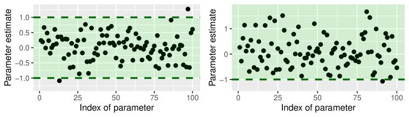
Figure 1: In some situations, e.g. food safety testing, one wants to show that many parameters lie in a certain interval or in a particular direction. In the figure on the left and on the right, the parameter estimates suggest that most parameters lie within the regions $(-1,1)$ and $(-1,\infty)$ respectively. In many such problems, based on prior knowledge, it is already expected that most parameters lie within such a region, and the goal is to corroborate that with data. This paper proposes powerful, nonparametric procedures that do this. In Sections 4-5, we select indices of parameters that seem to fall within the region, and estimate the number of incorrectly selected indices, i.e. the indices of parameters that in fact lie outside the region. In Section 6, we provide methods that select a set of indices such that the median of the fraction of incorrectly selected indices—i.e., the median of the FDP—stays below some chosen small value $\gamma\in[0,1)$.

In this paper, we propose novel multiple testing methods that are powerful in such situations. These methods connect to a large literature, which we review first, before discussing this paper’s contributions.

1.1 Existing multiple testing approaches

When multiple hypotheses are tested, the fraction of false discoveries among all rejected hypotheses is called the false discovery proportion (FDP). When there are no rejections, the FDP is defined to be 0. There exist a few different notions of FDP control. The oldest one is familywise error rate (FWER) control, which means guaranteeing that the FDP is 0 with high confidence (Goeman and Solari, 2014). Apart from FWER control, the most well-known notion is to control the expected value $\mathbb{E}(FDP)$, which is called the false discovery rate (FDR). FDR control means ensuring that $FDR\leq\gamma$, where $\gamma\in[0,1)$ is some user-specified bound (Benjamini and Hochberg, 1995; Benjamini and Yekutieli, 2001; Dickhaus, 2014; Wang and Ramdas, 2022).

Another manner of providing statements on the FDP is to fix some rejection region, reject all hypotheses with test statistics in this region and then provide a possibly data-dependent bound $\bar{FDP}$ for the FDP, which satisfies $\mathbb{P}(FDP\leq\bar{FDP})\geq 1-\alpha$. Here $\alpha\in(0,1)$ is a fixed, user-defined value, e.g. $0.05$. Permutation-based approaches for obtaining such bounds are provided in Hemerik and Goeman (2018b). A related goal is to guarantee that the $FDP$ is small with large probability, i.e. that $\mathbb{P}(FDP\leq\gamma)\geq 1-\alpha$, where $\gamma$ is chosen by the user. This is called false discovery exceedance control or FDX control. FDX controlling methods vary in the strictness of their assumptions and in the extent to which selective inference is allowed (van der Laan et al., 2004; Lehmann and Romano, 2005; Romano and Wolf, 2007; Guo and Romano, 2007; Farcomeni, 2008; Roquain, 2011; Guo et al., 2014; Delattre and Roquain, 2015; Javanmard and Montanari, 2018; Ditzhaus and Janssen, 2019; Hemerik et al., 2019; Katsevich and Ramdas, 2020; Blanchard et al., 2020; Döhler and Roquain, 2020; Basu et al., 2021; Goeman et al., 2021; Blain et al., 2022; Miecznikowski and Wang, 2023; Vesely et al., 2023). If we take $\gamma=0$, then we obtain FWER control.

FDX control provides an attractive statistical guarantee on the hypotheses that have been rejected. On the other hand, FDX methods tend to have relatively low power when $\gamma$ and $\alpha$ are small. For this reason, it can be useful to take $\alpha=0.5$. We then know that with probability at least $0.5$, the FDP is at most $\gamma$, i.e. $\mathbb{P}(FDP\leq\gamma)\geq 0.5$. This means that one controls the median of the FDP, or mFDP for short (Hemerik et al., 2024). mFDP control means that if the procedure is performed on many independent datasets, then the median of the resulting FDPs will be at most $\gamma$. Note that this is similar to FDR control; the only difference is that one controls the median instead of the mean.

1.2 Contributions

This paper focuses on the types of multiple testing problems discussed at the beginning of this Introduction, i.e., we consider one-sided or non-equivalence hypotheses, where it is expected that most hypotheses are false. For these settings, this paper proposes nonparametric mFDP controlling methods that are more powerful than existing exact mFDP and FDR methods. Our methods are built in such a way that they have good power when most parameters lie in their expected directions or intervals, which correspond to the alternative hypotheses. Our methods are valid for finite samples regardless of the actual parameters, but they only have good power if the user’s a priori expectations are mostly correct—which is usually the case in the applications we are interested in here. Our approach then tends to be superior in power, even compared to known exact mFDP procedures based on stepping down (Lehmann and Romano, 2005) or closed testing (Hemerik and Goeman, 2018b; Goeman et al., 2021; Hemerik et al., 2024). Of course, most multiple testing procedures become more powerful if appropriate one-sided tests instead of two-sided tests are used. However, our approach exploits such knowledge more effectively, in settings such as those in Figure 1.

The proposed methods are based computing a test statistic for every hypothesis and exploiting a natural symmetry property of the test statistics. For example, it is well know that test statistics are often asymptotically multivariate normal, so that they are asymptotically jointly symmetric about their means. Even if $n$ is finite and the test statistics are not normal then they are often still symmetric, as we will explain. The consequence of the symmetry property is that the joint distribution of the test statistics is unchanged when we reflect them about their means. We exploit reflected test statistics to derive a median unbiased estimator of the FDP, i.e., an estimator that underestimates the FDP with probability at most 0.5 (Hemerik et al., 2024). This is the same as a $50\%$-confidence upper bound for the FDP.

Later a procedure for mFDP control is proposed, which makes use of the mentioned FDP estimates. This mFDP controlling procedure evaluates the FDP estimates for different rejection regions, and then chooses a rejection region in such a way that the mFDP is at most $\gamma$. Since the FDP estimates used are not simultaneously valid $50\%$-confidence bounds, it is nontrivial to choose the rejection region in a way that leads to valid mFDP control. However, Theorem 6.1 states that this can be done. The manner of proving this result is new to our knowledge, since it is not based on closed testing or another familiar technique. Our methods are valid for finite samples and do not require independence.

1.3 Setup of this paper

In Section 2, we review some existing settings where nonparametric methods are useful. After discussing the case of a single hypothesis in Section 2.1, in Section 2.2 we discuss multiple testing and the method SAM, which is the main nonparametric competitor for FDP estimation.

After introducing our main assumption in Section 3, in Sections 4-5 we discuss median unbiased estimation of the FDP. For the case of one-sided testing—e.g., noninferiority testing—a novel method for median unbiased estimation of the FDP is in Section 4.1. Its admissibility is established in Section 4.2 and the method is conceptually compared to SAM in Section B of the Supplement. Section 5 defines a median unbiased FDP estimator for the case of equivalence testing.

In Section 6 we discuss control of the median of the FDP, i.e., methods which guarantee that $\mathbb{P}(FDP\leq\gamma)\geq 0.5$. The novel mFDP controlling method is discussed in Section 6.1 and implemented in the R package mFDP (Hemerik, 2025). This method builds on our median unbiased FDP estimates from Section 4 (directional testing) and Section 5 (equivalence testing). A link to the procedure in Hemerik et al. (2024) is discussed in Section 6.2. That method provides the flexibility of choosing $\gamma$ post hoc, but is less powerful than our novel method. Section 7 contains simulation and data analysis results. We end with a Discussion.

2 Existing nonparametric approaches

The methods proposed in this paper are nonparametric, in the sense that the stochastic part of the model is not assumed to follow some parametric distribution. They can be used in many settings where existing nonparametric multiple testing methods can also be used. The purpose of Section 2 is to gently introduce some of these settings and methods, which will be relevant in the rest of the paper. Firstly, in Section 2.1, we discuss examples of simple one-dimensional models, where basic nonparametric tests can be applied. These models will be extended to multiple testing settings in the examples in Section 3. In Section 2.2 we discuss multiple testing settings and corresponding nonparametric approaches for median unbiased estimation of the FDP. These will be compared to our novel approach conceptually in Section B of the Supplement and using simulation results in Section 7.1.

2.1 Testing a single hypothesis: examples

Nonparametric and semiparametric tests can be applied in many situations (Winkler et al., 2014; Canay et al., 2017; Hemerik et al., 2020; Berrett et al., 2020; Hemerik et al., 2021; Hemerik and Goeman, 2021; Dobriban, 2022; Liu et al., 2022; Zhang and Zhao, 2023). As with parametric tests, nonparametric tests are only exact for finite samples when the model is relatively simple. In this paper, we focus on methods that are valid for finite samples. Likewise, in this subsection, we limit ourselves to two examples of simple hypotheses with exact tests. Another example of an exact nonparametric test is a test of independence of two continuous variables (Neyman, 1942; DiCiccio and Romano, 2017; Kim et al., 2022).

2.1.1 Location model

Often we want to show that a population mean $\theta\in\mathbb{R}$ lies above some value $\delta\in\mathbb{R}$. In this case, the null hypothesis is $H_{0}:\theta\leq\delta$ and the alternative $H_{a}:\theta>\delta$. To test $H_{0}$, we might use a t-test. However, an advantage of a nonparametric approach is that it requires fewer assumptions. Moreover, nonparametric tests can be combined with powerful permutation-based multiple testing methods (Westfall and Young, 1993; Westfall and Troendle, 2008; Pesarin and Salmaso, 2010; Hemerik and Goeman, 2018b; Hemerik et al., 2019; Blain et al., 2022; Andreella et al., 2023). Fisher (1935, §21) introduces a nonparameric test based on sign-flipping. This test does not require normality, but instead requires the milder assumption that under $H_{0}$, the observations are symmetric about their mean. In particular, there is no homoscedastity assumption.

The model is the following. The data is a vector $X$ taking values in $\mathbb{R}^{n}$, where $n\geq 1$ is the sample size. The $n$ observations are assumed to be independent and to have the same mean $\theta$. Further, they are assumed to be symmetrically distributed about their mean under $H_{0}$. The observations can have different variances and distributions.

Note that without loss generality, we can assume that the null hypothesis is $H_{0}:\theta\leq 0$. To test $H_{0}$, one can consider the group of all sign-flipping transformations, i.e., all transformations $g:\mathbb{R}^{n}\rightarrow\mathbb{R}^{n}$ of the form $x\mapsto F_{g}x$, where $F_{g}$ is a diagonal matrix with diagonal elements in $\{-1,1\}$. There are $2^{n}$ such transformations $g$ and they form a group, say $\mathcal{G}$, in the algebraic sense (Hemerik and Goeman, 2018a; Koning and Hemerik, 2024). We refer to this group as the sign-flipping group. For every transformed data vector $F_{g}X$, the test computes the test statistic $T_{g}(X):=n^{-1/2}1_{n}^{\prime}F_{g}X$, where $1_{n}$ is the $n$-vector of ones. For the original data, the test statistic is

$$T_{id}(X)=n^{-1/2}1_{n}^{\prime}I_{n}X=n^{-1/2}\sum_{i=1}^{n}X_{i},$$

where $I_{n}$ is the $n\times n$ identity matrix. Given $\alpha\in(0,1)$, the test rejects $H_{0}:\theta\leq 0$ if and only if $T_{id}(X)$ is larger than $(1-\alpha)100\%$ of the other statistics. To make this formal, let $T^{(1)}(X)\leq...\leq T^{(|\mathcal{G}|)}(X)$ be the $|\mathcal{G}|=2^{n}$ sorted test statistics. Write $T^{(1-\alpha)}(X):=T^{\lceil(1-\alpha)|\mathcal{G}|\rceil}(X)$, where $\lceil c\rceil$ denotes the smallest integer than is at least as large as $c$. Then the test rejects if and only if

$$T_{id}(X)>T^{(1-\alpha)}(X),$$ (1)

It is well known that this test has type I error rate at most $\alpha$ (Arboretti et al., 2021), although most literature assumes a point null hypothesis.

Theorem 2.1.

Consider $X$ as above and $H_{0}:\theta\leq 0$. The test that rejects when inequality (1) holds, satisfies $\mathbb{P}_{H_{0}}(\text{reject }H_{0})\leq\alpha$. Further, if $\theta=0$ and $\alpha$ is a multiple of $|G|^{-1}$ and $X$ is continuous, then $\mathbb{P}_{H_{0}}(\text{reject }H_{0})=\alpha$.

2.1.2 Comparing two groups

Another nonparametric model relevant to this paper is the following one, often used for comparing two populations by exact permutation testing. Consider two samples $Z$ and $Y$, which both take values in $\mathbb{R}^{n}$. Here $Z$ usually represents a sample from one population and $Y$ a sample from another population. The assumption that both samples are equally large is made for convenience. We write the whole dataset as $X=(Z^{\prime},Y^{\prime})^{\prime}$. The permutation test employs permutation maps $g:\mathbb{R}^{2n}\rightarrow\mathbb{R}^{2n}$. A permutation map is a transformation of the form $(x_{1},...,x_{2n})^{\prime}\mapsto(x_{\pi(1)},...,x_{\pi({2n})})^{\prime}$, where $(\pi(1),...,\pi({2n}))$ is a permutation of $(1,...,2n)$. Note that there are $(2n)!$ such permutation maps.

As a concrete example, suppose that all $2n$ observations are i.i.d., except that the observations in $Z$ have mean $\theta^{1}$ and the observations in $Y$ have mean $\theta^{2}$. Then we can test the null hypothesis $H_{0}:\theta\leq\delta$, where $\theta=\theta^{1}-\theta^{2}$. Without loss of generality we can assume that $\delta=0$. To test $H_{0}$, we compute the test statistic

$$T(X)=T_{id}(X)=T\{(Z^{\prime},Y^{\prime})^{\prime}\}:=n^{1/2}(\bar{Z}-\bar{Y}),$$

where $\bar{Z}$ denotes the mean of the entries of $Z$ and likewise for $Y$. Letting $\mathcal{G}$ be the group of $(2n)!$ permutation maps, for every $g\in\mathcal{G}$ we compute the test statistic $T_{g}(X)=T(g(X))$. As in section 2.1.1, we define $T^{(1-\alpha)}(X)$ to be the $(1-\alpha)$-quantile of these test statistics and reject $H_{0}$ if and only if $T(X)>T^{(1-\alpha)}(X)$. As a sidenote, it can be seen that many permutations lead to the same test statistic, so that in fact we only need to use $\binom{2n}{n}$ permutations (Hemerik and Goeman, 2018a), which speeds up the computation.

It is well-known that this test controls the type I error rate (Pesarin, 2015), although this is usually proved for the case of a point null hypothesis (Hoeffding, 1952; Lehmann and Romano, 2022; Hemerik and Goeman, 2018a).

Theorem 2.2.

Consider $X=(Z^{\prime},Y^{\prime})^{\prime}$ as above. Suppose that all $2n$ observations are i.i.d., except that the observations in $Z$ have mean $\theta^{1}$ and the observations in $Y$ have mean $\theta^{2}$. Consider $H_{0}:\theta\leq 0$, where $\theta=\theta^{1}-\theta^{2}$. Consider the test that rejects when inequality (1) holds, which is now understood to refer to the current setting. This test satisfies $\mathbb{P}_{H_{0}}(\text{reject }H_{0})\leq\alpha$. Further, in case $\theta=0$ and $\alpha$ is a multiple of $\binom{2n}{n}$ and $X$ is continuous, then $\mathbb{P}_{H_{0}}(\text{reject }H_{0})=\alpha$.

Remark 1.

For what follows later (e.g. Section 3), it is important to realize that in the setting of Theorem 2.2, the test statistic $T(X)=n^{1/2}(\bar{Z}-\bar{Y})$ is symmetric about its mean $n^{1/2}\theta$, even if the $2n$ variables are not symmetric. To see this, note that $(\bar{Z}-\bar{Y})$ is symmetric about $\theta$, which follows from

$$(\bar{Z}-\bar{Y})-\theta=(\bar{Z}-\theta^{1})-(\bar{Y}-\theta^{2})\,{\buildrel d\over{=}}\,(\bar{Y}-\theta^{2})-(\bar{Z}-\theta^{1})=\theta-(\bar{Z}-\bar{Y}),$$

where we used that $(\bar{Z}-\theta^{1})\,{\buildrel d\over{=}}\,(\bar{Y}-\theta^{2})$ by assumption, as well as independence of $\bar{Z}$ and $\bar{Y}$.

2.2 Existing nonparametric methods for FDP estimation

Sections 4-5 of this paper are about median unbiased estimators of the FDP, i.e., estimators $\bar{FDP}$ satisfying

$$\mathbb{P}(FDP\leq\bar{FDP})\geq 0.5.$$ (2)

In this section we review the main nonparametric competitors of our novel mFDP estimators, namely the permutation methods in Hemerik and Goeman (2018b).

Hemerik and Goeman (2018b) contains a fast method, which we will refer to as SAM, and a more powerful but much slower procedure, which we will refer to as SAM+CT. Here SAM stands for “Significance Analysis of Microarrays”, however the methodology is very general and not at all limited to microarray data. Further, “CT” stands for closed testing, which is a fundamental principle for constructing admissible multiple testing procedures (Genovese and Wasserman, 2006; Goeman and Solari, 2011; Goeman et al., 2021). One message of this paper is that in the settings we are interested here, our estimators perform better than SAM and SAM+CT—in the sense that our estimates of the FDP tend to be smaller.

Since the comparison of our estimators with SAM and SAM+CT is an important part of this paper, we summarize these methods here. Let $X$ be data, taking values in a sample space $\mathcal{S}$. Consider null hypotheses $H_{1},...,H_{m}$ and corresponding test statistics $T_{j}:\mathcal{S}\rightarrow\mathbb{R}$, $1\leq j\leq m$, which may be dependent. Hemerik and Goeman (2018b) considers quite general rejection regions which can depend on $1\leq j\leq m$, but for simplicity we will assume the following rejection rule: we reject all hypotheses $H_{j}$ with $T_{j}(X)>t$, where $t\geq 0$ is some prespecified value. This means that the set of indices of the rejected hypotheses is

$$\mathcal{R}(t)=\mathcal{R}(X,t)=\{1\leq j\leq m:T_{j}(X)>t\}.$$

We will often refrain from writing the argument $X$ or $t$ when it is clear from the context. Write $R(t)=R(X,t)=|\mathcal{R}(t)|$ and let

$$\mathcal{N}=\{1\leq j\leq m:H_{j}\text{ is true}\},$$

which we assume to be nonempty for convenience. The number of false positive discoveries is then $V(t)=|\mathcal{N}\cap\mathcal{R}(t)|$ and the FDP is

$$FDP(t)=V(t)/(R(t)\vee 1).$$

Let $\mathcal{G}$ be a set of transformations $g:\mathcal{S}\rightarrow\mathcal{S}$, such that $\mathcal{G}$ is a group under composition of maps (Hemerik and Goeman, 2018b). Here $\mathcal{G}$ may for example consist of sign-flipping maps or permutation maps as in Section 2.1—the difference being that here the group typically acts on a whole data matrix, e.g. it may simultaneously sign-flip or permute the data. The main assumption from Hemerik and Goeman (2018b) is Assumption 1 below. An example where this assumption holds is given under Assumption 1 in Hemerik and Goeman (2018b, p.139).

Assumption 1.

The joint distribution of the test statistics $T_{j}\{g(X)\}$ with $j\in\mathcal{N}$ and $g\in\mathcal{G}$ is invariant under all transformations in $\mathcal{G}$ of $X$.

SAM then considers the permutation distribution of the number of rejections. That is, let $R^{(1)}\leq...\leq R^{(|\mathcal{G}|)}$ be the sorted values $R(g(X),t)$, $g\in\mathcal{G}$. Now define

$$\bar{V}(t)=\bar{V}(X,t):=\min\{R^{(\lceil(1-\alpha)|\mathcal{G}|\rceil)},R\},$$

i.e., the minimum of $R(X,t)$ and the $(1-\alpha)$-quantile of the values $R(g(X),t)$, $g\in\mathcal{G}$. If $\alpha=0.5$, this means taking the median of those values. Theorem 2 in Hemerik and Goeman (2018b) states that $\mathbb{P}(V(t)\leq\bar{V}(t))\geq 1-\alpha$, which for $\alpha=0.5$ translates to

$$\mathbb{P}(V(t)\leq\bar{V}(t))\geq 0.5.$$

Defining

$$\bar{FDP}(t)=\bar{V}(t)/(R(t)\vee 1)$$

gives a bound $\bar{FDP}(t)$ satisfying inequality (2).

As noted in Hemerik and Goeman (2018b), the bound $\bar{FDP}(t)$ can be uniformly improved, while still guaranteeing that inequality (2) holds. Indeed, $\bar{FDP}(t)$ is uniformly improved by a bound based on closed testing. This bound is provided in Proposition 1 of Hemerik and Goeman (2018b) and in that paper the details are given. This is the method that we will refer to as SAM+CT. Intuitively, the idea is that especially when there are many false hypotheses, the basic SAM method will be conservative because the many false hypotheses cannot lead to false discoveries. SAM+CT addresses that issue.

As discussed in Section B of the Supplement and in 7.1, our novel FDP estimator does not uniformly improve SAM+CT, but on average it povides lower FDP estimates, for the scenarios that we are interested in here. Another crucial advantage of our novel method is that it is much faster than SAM+CT. Whereas the computation time of SAM+CT is typically more than exponential in $m$, the computation time of the novel method in linear in $m$. In practice SAM+CT is only computationally feasible for quite small multiple testing problems ($m\leq 100$).

3 Main assumption of this paper

In this paper we study multiple hypothesis testing problems of the following form. Consider hypotheses $H_{1},...,H_{m}$ and corresponding test statistics $T_{1},...,T_{m}$ with means $\mu_{1},...,\mu_{m}\in\mathbb{R}$ respectively. These test statistics might e.g. be unbiased estimators of certain parameters $\theta_{1},...,\theta_{m}$ of interest, in which case we simply have $\mu_{j}=\mathbb{E}(T_{j})=\theta_{j}$, $1\leq j\leq m$. Throughout Sections 4 and 4.2 we suppose that for every $1\leq j\leq m$ the null hypothesis is

$$H_{j}:\mu_{j}\leq\delta_{j},$$ (3)

where $\delta_{1},...,\delta_{m}\in\mathbb{R}$ are constants. Testing non-equivalence hypotheses of the form

$$H_{j}:|\mu_{j}|\geq\delta_{j}$$

will be covered in Section 5.

Throughout the rest of this paper, we will assume that the test statistics $T_{1},...,T_{m}$ satisfy the following symmetry property. In fact, it is only an assumption on the joint distribution of $(T_{j}:i\in\mathcal{N})$, i.e., the test statistics corresponding to the true hypotheses.

Assumption 2.

The vector $(T_{j}-\mu_{i}:i\in\mathcal{N})$ is nondegenerate and satisfies

$$(T_{j}-\mu_{j}:j\in\mathcal{N})\,{\buildrel d\over{=}}\,(-(T_{j}-\mu_{j}):j\in\mathcal{N}).$$

The above assumption is valid in many situations. For example, if the statistics $(T_{j}:i\in\mathcal{N})$ are multivariate normal, then the assumption is satisfied. However, we do not need normality. Here are two basic examples where Assumption 2 is satisfied.

Example (Nonparametric location model).

In Section 2.1.1 we considered a non-parametric location model and a hypothesis test. Now consider not one such test, but $m$ such hypotheses and tests. Now $X$ is not an $n$-vector but an $n$-by-$m$ matrix $X=(X^{1},...,X^{m})$, where $X^{j}$ is an $n$-vector whose entries have mean $\theta_{j}$, $1\leq j\leq m$. For every $1\leq j\leq m$ we now consider the null hypothesis $H_{j}:\theta_{j}\leq\delta$ and define $T_{j}=n^{-1}1_{n}^{\prime}X^{j}$. Note that $\mu_{j}=\mathbb{E}(T_{j})=\theta_{j}$ and $\mathcal{N}=\{1\leq j\leq m:\theta_{j}\leq\delta\}$. Let $X^{\mathcal{N}}$ be the $n$-by-$|\mathcal{N}|$ submatrix $(X^{j}:j\in\mathcal{N})$ and write $X^{\mathcal{N}}_{i}$ for its $i$-th row. Assume that the rows of $X^{\mathcal{N}}$ are independent of each other. Within each row, there may be dependence. Let $\theta^{\mathcal{N}}:=(\theta_{j}:j\in\mathcal{N})$ and assume that for every $1\leq i\leq n$, the rows of $X^{\mathcal{N}}-\theta^{\mathcal{N}}$ are symmetric, i.e. that $X^{\mathcal{N}}_{i}-\theta^{\mathcal{N}}\,{\buildrel d\over{=}}\,-(X^{\mathcal{N}}_{i}-\theta^{\mathcal{N}})$.

Note that the entries $(T_{j}-\mu_{j}:j\in\mathcal{N})$ have mean $0$ and satisfy

$$(T_{j}-\mu_{j}:j\in\mathcal{N})=$$

$$\big{\{}(n^{-1}1_{n}^{\prime}X^{j}-\theta_{j}):j\in\mathcal{N}\big{\}}=$$

$$\big{\{}n^{-1}(1_{n}^{\prime}X^{j}-n\theta_{j}):j\in\mathcal{N}\big{\}}=$$

$$\big{\{}n^{-1}\sum_{1\leq i\leq n}(X_{i}^{j}-\theta_{j}):j\in\mathcal{N}\big{\}}.$$

Since the rows of $X^{\mathcal{N}}$ are symmetric and independent of each other, this is equal in distribution to

$$\big{\{}n^{-1}\sum_{1\leq i\leq n}(-(X_{i}^{j}-\theta_{j})):j\in\mathcal{N}\big{\}}=$$

$$\big{\{}n^{-1}(-(1_{n}^{\prime}X^{j}-n\theta_{j})):j\in\mathcal{N}\big{\}}=$$

$$(-(T_{j}-\mu_{j}):j\in\mathcal{N}),$$

so that Assumption 2 is satisfied.

In the example above we assumed that the observations are symmetric. In the example below, we do not make such an assumption, yet still the test statistics satisfy Assumption 2.

Example (Comparing two groups).

We now extend the setting of Section 2.1.2 to the case of multiple hypotheses; here we will also see that Assumption 2 is satisfied. Now $X$ is a $2n$-by-$m$ matrix $X=(X^{1},...,X^{m})$, where for each $1\leq j\leq m$, $X^{j}=(Z^{j^{\prime}},Y^{j^{\prime}})^{\prime}$ is a $2n$-dimensional column vector, where $Z^{j}$ is the j-th column of an $n$-by-$m$ matrix $Z$ and $Y^{j}$ is the j-th column of an $n$-by-$m$ matrix $Y$. For $1\leq j\leq m$, the entries of $Z^{j}$ have mean $\theta^{1}_{j}$ and the entries of $Y^{j}$ have mean $\theta^{2}_{j}$. For every $1\leq j\leq m$, consider the null hypothesis $H_{j}:\theta_{j}\leq\delta$, where $\theta_{j}=\theta^{1}_{j}-\theta^{2}_{j}$. For each $1\leq j\leq m$, let $T_{j}=n^{1/2}(\bar{Z}^{j}-\bar{Y}^{j})$, where $\bar{Z}^{j}$ is the mean of the entries of ${Z}^{j}$ and likewise for ${Y}^{j}$. Note that $\mu_{j}:=\mathbb{E}(T_{j})=n^{1/2}(\theta^{1}_{j}-\theta^{2}_{j})=n^{1/2}\theta_{j}$. Let $X^{\mathcal{N}}$ be the $n$-by-$|\mathcal{N}|$ submatrix $(X_{j}:j\in\mathcal{N})$. Assume that the rows of $X^{\mathcal{N}}$ are independent of each other and each have the same joint distribution, apart from a mean shift so that the columns of $Z$ and $Y$ have the means specified above. Within each row, there may be dependence. Thus, the matrices $Z^{\mathcal{N}}$ and $Y^{\mathcal{N}}$ have the same joint distribution, except that the columns of $Z^{\mathcal{N}}$ can have different means than the columns of $Y^{\mathcal{N}}$.

Note that the entries $(T_{j}-\mu_{j}:j\in\mathcal{N})$ have mean $0$ and satisfy

$$(T_{j}-\mu_{j}:j\in\mathcal{N})=$$

$$\big{\{}n^{1/2}(\bar{Z}^{j}-\bar{Y}^{j})-n^{1/2}\theta_{j}:j\in\mathcal{N}\big{\}}=$$

$$\Big{\{}n^{1/2}\big{(}(\bar{Z}^{j}-\theta_{j}^{1})-(\bar{Y}^{j}-\theta_{j}^{2})\big{)}:j\in\mathcal{N}\Big{\}}=$$

$$\Big{\{}n^{1/2}n^{-1}\sum_{1\leq i\leq n}\big{(}({Z}_{i}^{j}-\theta_{j})-({Y}_{i}^{j}-\theta_{j}^{2})\big{)}:j\in\mathcal{N}\Big{\}}=$$

$$n^{1/2}n^{-1}\sum_{1\leq i\leq n}\Big{\{}({Z}_{i}^{j}-\theta_{j})-({Y}_{i}^{j}-\theta_{j}^{2}):j\in\mathcal{N}\Big{\}}.$$ (4)

Note that for every $1\leq i\leq n$,

$$\big{\{}({Z}_{i}^{j}-\theta_{j}^{1})-({Y}_{i}^{j}-\theta_{j}^{2}):j\in\mathcal{N}\big{\}}\,{\buildrel d\over{=}}\,$$

$$\big{\{}({Y}_{i}^{j}-\theta_{j}^{2})-({Z}_{i}^{j}-\theta_{j}^{1}):j\in\mathcal{N}\big{\}},$$

where we used that

$$(Z^{j}_{i}-\theta^{1}_{j}:j\in\mathcal{N})\,{\buildrel d\over{=}}\,(Y^{j}_{i}-\theta^{2}_{j}:j\in\mathcal{N})$$

combined with the fact that the rows of $X$ are mutually independent.

Hence, (4) is equal in distribution to

$$n^{1/2}n^{-1}\sum_{1\leq i\leq n}\Big{\{}\big{(}({Y}_{i}^{j}-\theta_{j}^{2})-({Z}_{i}^{j}-\theta_{j})\big{)}:j\in\mathcal{N}\Big{\}}=$$

$$\Big{\{}n^{1/2}\big{(}(\bar{Y}^{j}-\theta_{j}^{2})-(\bar{Z}^{j}-\theta_{j}^{1})\big{)}:j\in\mathcal{N}\Big{\}}=$$

$$\Big{\{}n^{1/2}(\bar{Y}^{j}-\bar{Z}^{j})+n^{1/2}\theta_{j}:j\in\mathcal{N}\Big{\}}=$$

$$(-(T_{j}-\mu_{j}):j\in\mathcal{N}),$$

so that Assumption 2 is satisfied.

Remark 2.

Note that in Example Example, we assumed that the rows of the data matrix $X$ were independent of each other. While this is a common assumption, it is in fact not needed at all for Assumption 2 to be satisfied. Indeed, it suffices to assume that the matrices $Z^{\mathcal{N}}$ and $Y^{\mathcal{N}}$ have the same joint distribution after removing the means of their entries. The reason is that Assumption 2 is quite mild. In particular, we do not need invariance under all permutations like SAM does.

Remark 3.

In Example Example, the hypotheses were $H_{j}:\theta_{j}\leq\delta$. This can straightforwardly be generalized to the more general collection of hypotheses $H_{j}^{\prime}:\theta_{j}\leq\delta_{j}$, where $\delta_{1},...,\delta_{m}\in\mathbb{R}$. Indeed, for every $1\leq j\leq m$ we can shift, i.e. translate, the observations in $Z^{j}$ by $\delta-\delta_{j}$. Then $H_{j}$ holds for the shifted data if and only if $H_{j}^{\prime}$ holds for the original data. Likewise, we can generalize to the situation where some of the hypotheses are of the form $H_{j}^{\prime\prime}:\theta_{j}\geq\delta_{j}$, with a left-sided alternative. Indeed, if we multiply the corresponding columns of $X$ by $-1$ and then suitably shift the data, the problem becomes that of Example Example.

4 FDP estimator for one-sided tests

In this section we cover our median unbiased FDP estimator for the case of one-sided tests. Besides being useful in its own right, the estimator will be used by the mFDP controlling method from Section 6.1. The estimator is defined in Section 4.1. In Section 4.2 it is proven that it is admissible, i.e., it cannot be uniformly improved by a different median unbiased estimator.

4.1 Definition of the estimator

Pick $t\geq 0$ and for every $1\leq j\leq m$, let $\delta_{j}\geq 0$. Consider hypotheses of the form (3). Reject the hypotheses with indices in

$$\mathcal{R}(t)=\mathcal{R}((T_{1},...,T_{m}),t)=\{1\leq j\leq m:T_{j}-\delta_{j}>t\}.$$

Instead of $\mathcal{R}((T_{1},...,T_{m}),t)$, we will often write $\mathcal{R}(t)$ or $\mathcal{R}$ when it is clear from the context that the arguments are $(T_{1},...,T_{m})$ and $t$. The number of false discoveries that the new method makes is $V=V(t)=\mathcal{N}\cap\mathcal{R}(t)$, where we used the notation introduced in Section 2.2. Also recall the notation $R=|\mathcal{R}|$. Write $a_{1}\wedge a_{2}$ for the minimum of two numbers $a_{1}$ and $a_{2}$. The novel estimator for the number of false positives is defined as

$$\tilde{V}(t)=R^{-}(t)\wedge R(t),$$

where $R^{-}(t)=|\mathcal{R}^{-}(t)|$ with

$$\mathcal{R}^{-}(t):=\{1\leq j\leq m:T_{j}-\delta_{j}<-t\}.$$

Analogously, the novel FDP estimator is defined to be

$$\tilde{FDP}(t)=\tilde{V}(t)/(R(t)\vee 1).$$

The way in which we thus estimate the FDP may bring to mind the knockoffs procedure from the seminal work Barber and Candès (2015). However, a difference is that the test statistics based on knockoffs are mutually independent, whereas here they need not be.

We will first show that under Assumption 2, these estimators are median unbiased, i.e., they satisfy

$$\mathbb{P}(V(t)\leq\tilde{V}(t))\geq 0.5,$$ (5)

or equivalently,

$$\mathbb{P}(FDP(t)\leq\tilde{FDP}(t))\geq 0.5.$$ (6)

Theorem 4.1.

Under Assumption 2, the bound $\tilde{FDP}$ satisfies equation (6).

The estimator $\tilde{V}$ is compared with SAM in Section B of the Supplement. There, a related result is discussed as well, namely that if $\alpha=0.5$, using a very small number of permutations in SAM may improve its power, which is a surprising result.

We now investigate whether the estimator $\tilde{V}(t)$ is admissible, i.e., whether it can be uniformly improved, without violating requirement (5). Assume for a moment that $\mu_{j}=\delta_{j}$ for all $1\leq j\leq m$, so that all hypotheses are true, but barely so. Then we can note the following.

Lemma 4.2.

Suppose Assumption 2 holds and $\mu_{j}=\delta_{j}$ for all $1\leq j\leq m$. Hence $V(t)=R(t)$. Define the events

$$E_{1}=\{V(t)<R^{-}(t)\}=\{R(t)<R^{-}(t)\},$$

$$E_{2}=\{V(t)=R^{-}(t)\}=\{R(t)=R^{-}(t)\},$$

$$E_{3}=\{V(t)>R^{-}(t)\}=\{R(t)>R^{-}(t)\}.$$

Then $\mathbb{P}(E_{1})=\mathbb{P}(E_{3})$ and $\mathbb{P}(E_{1})=0.5-0.5\mathbb{P}(E_{2})$.

Thus, in the scenario of Lemma 4.2, we will only have $\mathbb{P}(E_{1})=0.5$ if $\mathbb{P}(E_{2})=0$, which is however typically not the case—although it is often approximately true when there are many hypotheses. In conclusion, $\mathbb{P}(E_{3})$ is typically strictly smaller than $0.5$ and consequently $\mathbb{P}(V(t)>\tilde{V}(t))$ is typically strictly smaller than $0.5$. It can be seen that this is also the case for other values of $\delta_{1},...,\delta_{m}$.

This suggests to slightly adapt the procedure in the situation that $R(t)$ and $\tilde{V}(t)$ are tied, in order to have a method that can be shown to be admissible. Indeed, consider the following adapted bound $\tilde{V}^{\prime}$:

$$\tilde{V}^{\prime}(t)=\begin{cases}d&\text{if }R(t)=R^{-}(t)\\ \tilde{V}(t)&\text{otherwise,}\end{cases}$$

where $d$ is an independent variable that equals $\tilde{V}(t)$ or $-\infty$ both with probability $0.5$. This procedure sets the bound to $-\infty$ with probability 0.5 when $R(t)=R^{-}(t)$. Since the bound $\tilde{V}^{\prime}(t)$ is based on a random coin flip $d$, we do not recommend using $\tilde{V}^{\prime}(t)$ in practice. However, we will show that $\tilde{V}^{\prime}(t)$ is admissible. Since typically $\tilde{V}(t)=\tilde{V}^{\prime}(t)$ with high probability when there are many rejected hypotheses, it follows that $\tilde{V}$ is essentially admissible for most practical purposes.

The following result states that the bound $\tilde{V}^{\prime}(t)$ is valid. Admissibility of $\tilde{V}^{\prime}(t)$ is shown in Section 4.2.

Proposition 4.3.

Suppose Assumption 2 holds. The bound $\tilde{V}^{\prime}(t)$ is median unbiased in the sense that $\mathbb{P}\{V(t)\leq\tilde{V}^{\prime}(t)\}\geq 0.5.$ Further, in case $\mu_{j}=\delta_{j}$ for all $1\leq j\leq m$, we have $\mathbb{P}\{V(t)\leq\tilde{V}^{\prime}(t)\}=0.5$.

Proposition 4.3 implies that in some cases $\mathbb{P}\{V(t)\leq\tilde{V}^{\prime}(t)\}=0.5=\alpha$, i.e., in some cases $\tilde{V}^{\prime}(t)$ exhausts $\alpha$. However, this does not yet imply that $\tilde{V}^{\prime}(t)$ is admissible. Indeed, multiple testing methods that exhaust $\alpha$ when $\mathcal{N}=\{1,...,m\}$, are not always admissible. For example, Bonferroni also exhausts $\alpha$ in certain situations where $\mathcal{N}=\{1,...,m\}$, yet it is not admissible since it is uniformly improved by Bonferroni-Holm (Holm, 1979; Goeman and Solari, 2014). Likewise, a simple single-step FWER method based on Simes’ inequality can exhaust $\alpha$ when $\mathcal{N}=\{1,...,m\}$, yet it is uniformly improved by Hommel’s method (Hommel, 1988; Goeman and Solari, 2014). Nevertheless, it turns out that the simple estimator $\tilde{V}^{\prime}(t)$ is admissible, which we show in Section 4.2.3.

4.2 Closed testing and admissibility

In this section, we link the bounds $\tilde{V}$ and $\tilde{V}^{\prime}$ to the theory of closed testing and prove that the bound $\tilde{V}^{\prime}$ is admissible, i.e., that it cannot be uniformly improved.

4.2.1 General construction of FDP bounds using closed testing

We start by reviewing what closed testing is and how it can be used to obtain bounds $B$ of the form $\mathbb{P}(V\leq B)\geq 1-\alpha$, where $\alpha\in(0,1)$ is fixed in advance. The closed testing principle goes back to Marcus et al. (1976) and can be used to construct multiple testing procedures that control the family-wise error rate (Sonnemann, 2008; Romano et al., 2011). Goeman and Solari (2011) show that such procedures can be extended to provide confidence bounds for the numbers of true hypotheses in all sets of hypotheses simultaneously (an equivalent approach is in Genovese and Wasserman, 2006).

Let $\mathcal{C}$ be the collection of all nonempty subsets of $\{1,...,m\}$. For every $I\in\mathcal{C}$ consider the intersection hypothesis $H_{I}=\cap_{i\in I}H_{i}$. This is the hypothesis that all $H_{i}$ with $i\in I$ are true. For every $I\in\mathcal{C}$, consider some local test $\phi_{I}$, which is $1$ if $H_{I}$ is rejected and $0$ otherwise. Assume the test $\phi_{\mathcal{N}}$ is valid in the sense that it has level at most $\alpha$, i.e., $\mathbb{P}(\phi_{\mathcal{N}}\geq 1)\leq\alpha$. Since we do not know $\mathcal{N}$, this effectively means that we require all the local tests to be valid. A closed testing procedure generally rejects all intersection hypotheses $H_{I}$ with $I\in\mathcal{X}$, where

$$\mathcal{X}=\{I\in\mathcal{C}:\phi_{J}=1\text{ for all }I\subseteq J\subseteq\{1,...,m\}\}.$$

It is well-known that this procedure controls the familywise error rate (Marcus et al., 1976), i.e., with probability at least $1-\alpha$ there are 0 type I errors. In Goeman and Solari (2011) it is shown that we can also use the set $\mathcal{X}$ to provide a $(1-\alpha)$-confidence upper bound for the number of true hypotheses in any $I\in\mathcal{C}$. They show that

$$t_{\alpha}(I):=\max\{|J|:J\subseteq I\text{ and }J\not\in\mathcal{X}\}.$$

is a $(1-\alpha)$-confidence upper bound for $|\mathcal{N}\cap I|$. In fact, they show that the bounds $t_{\alpha}(I)$ are valid simultaneously over all $I\in\mathcal{C}:$

$$\mathbb{P}\Bigg{[}\bigcap_{I\in\mathcal{C}}\Big{\{}|\mathcal{N}\cap I|\leq t_{\alpha}(I)\Big{\}}\Bigg{]}\geq 1-\alpha.$$ (7)

The proof is short: with probability at least $1-\alpha$, $H_{\mathcal{N}}$ is not rejected by its local test. In case $H_{\mathcal{N}}$ is not rejected by its local test, for every $I\in\mathcal{C}$ it holds that $|\mathcal{N}\cap I|\not\in\mathcal{X}$, so that $|\mathcal{N}\cap I|\leq t_{\alpha}(I)$, i.e., $t_{\alpha}(I)$ is a valid upper bound for the number of true hypotheses in $I$. This proves inequality (7). A different method, formulated in Genovese and Wasserman (2006), leads to the same bounds. The two approaches were compared in the supplementary material of Hemerik et al. (2019).

4.2.2 $\tilde{V}$ coincides with a closed testing method

We first consider the bound $\tilde{V}$. We will define local tests and, as explained in Section 4.2.1, use closed testing to obtain bounds. Then we show that these bounds are equivalent with $\tilde{V}$, so that $\tilde{V}$ coincides with a closed testing procedure.

Recall the definition of $\mathcal{C}$ from Section 4.2.1. For every $I\in\mathcal{C}$, we will define a corresponding local test $\tilde{\phi}_{I}$. First define

$$R_{I}(t):=|I\cap\mathcal{R}(t)|=\{j\in I:T_{j}>\delta_{j}+t\},$$

$$R^{-}_{I}(t):=|I\cap\mathcal{R}^{-}(t)|=\{j\in I:T_{i}<\delta_{j}-t\}.$$

Again, we will often refrain from writing “$(t)$” for brevity. For every $I\in\mathcal{C}$, we define the local test

$$\tilde{\phi}_{I}=\mathbbm{1}(R_{I}>R^{-}_{I}),$$ (8)

where $\mathbbm{1}(\cdot)$ is the indicator function.

Proposition 4.4.

Suppose Assumption 2 holds. Then for every $I\in\mathcal{C}$, the local test $\tilde{\phi}_{I}$ is valid for $\alpha=0.5$, in the sense that if $H_{I}$ is true, then $\mathbb{P}(\tilde{\phi}_{I}=1)\leq 0.5.$

We now investigate which $I$ is in $\mathcal{X}$, i.e, which intersection hypotheses are rejected by the closed testing procedure.

Proposition 4.5.

Consider the closed testing procedure based on the local tests defined by equation (8). For any $I\in\mathcal{C}$, we have $I\in\mathcal{X}$ if and only if $R_{I}>R^{-}$, where we recall that $R^{-}=R^{-}_{\{1,...,m\}}$.

Next we investigate what bounds the above closed testing procedure provides. For $I\in\mathcal{C}$, note that

$$t_{\alpha}(I)=\max\{|J|:J\subseteq I\text{ and }J\not\in\mathcal{X}\}=$$

$$\max\{|J|:J\subseteq I\text{ and }R_{J}\leq R^{-}\}.$$ (9)

In particular, we are interested in $t_{\alpha}(\mathcal{R}(t))=t_{\alpha}(\mathcal{R})$, since this provides a bound for $|\mathcal{N}\cap\mathcal{R}(t)|=V(t)$, which is the number of incorrect rejections for our method defined in Section 4.1. Note that

$$t_{\alpha}(\mathcal{R}(t))=\max\{|J|:J\subseteq\mathcal{R}\text{ and }R_{J}\leq R^{-}\}=$$

$$\max\{|J|:J\subseteq\mathcal{R}\text{ and }|J|\leq R^{-}\}=R\wedge R^{-}=\tilde{V}(t).$$

Thus, $\tilde{V}(t)$ concides with the $50\%$-confidence bound for $|\mathcal{N}\cap\mathcal{R}|$ produced by this closed testing procedure. Now consider any other $I\in\mathcal{C}$. Expression (9) can be rewritten as

$$|I|\wedge\big{(}|\{j\in I:T_{j}\leq\delta_{j}+t\}|+R^{-}\big{)}=|I|\wedge\big{(}|I\cap\mathcal{R}^{c}|+R^{-}\big{)},$$

where $\mathcal{R}^{c}:=\{1,...,m\}\setminus\mathcal{R}$. Thus, the $50\%$-confidence bound for the number of true hypotheses in $I$, $|\mathcal{N}\cap I|$, is simply the bound $R^{-}$ for $|\mathcal{N}\cap\mathcal{R}|$ plus the number of elements in $I$ that are not in $\mathcal{R}$. But this bound follows trivially from the bound $\tilde{V}=R^{-}\wedge R$ for $|\mathcal{N}\cap R|$, without looking at the data. Thus, all the information contained in the bounds $t_{\alpha}(I)$, $I\in\mathcal{C}$, is already contained in our single bound $\tilde{V}$. Thus, the bound $\tilde{V}$ is completely equivalent to the bounds from the closed testing procedure. As we showed, $\tilde{V}$ is not admissible—since it is improved by $\tilde{V}^{\prime}$—and hence this closed testing procedure is not admissible.

4.2.3 $\tilde{V}^{\prime}$ is admissible

Next, we will show that $\tilde{V}^{\prime}$ also coincides with a closed testing procedure and that that procedure is admissible. We will then deduce that $\tilde{V}^{\prime}$ is admissible. We start by defining the closed testing procedure, which we do by defining its local tests. For every $I\in\mathcal{C}$, we define the local test

$$\tilde{\phi}^{\prime}_{I}=\begin{cases}1&\text{if }R_{I}(t)>R_{I}^{-}(t)\\ b&\text{if }R_{I}(t)=R_{I}^{-}(t)\\ 0&\text{otherwise,}\end{cases}$$ (10)

i.e.,

$$\tilde{\phi}^{\prime}_{I}=\mathbbm{1}(R_{I}>R_{I}^{-})+b\mathbbm{1}(R_{I}=R_{I}^{-}),$$

where we define $b$ to be a coin flip satisfying $b=1$ when $d=-\infty$ and $b=0$ if $d=1$. Note that $\tilde{\phi}^{\prime}_{I}$ is a valid local tests for $\alpha=0.5$, i.e., if $H_{I}$ is true then $\mathbb{P}(\tilde{\phi}^{\prime}_{I}=1)\leq 0.5.$

We first show that this test exhausts $\alpha=0.5$, under some distributions.

Lemma 4.6.

For every $I\in\mathcal{C}$, there exists a distribution of $(T_{1},...,T_{m})$ for which 1. Assumption 2 is satisfied, 2. $H_{I}$ is true and 3. $\mathbb{P}(\tilde{\phi}^{\prime}_{I}=1)=0.5$.

In many situations, if a test exhausts $\alpha$ under some distributions, then it is admissible. The lemma below states that this is also the case for the local tests $\tilde{\phi}^{\prime}_{I}$, $I\in\mathcal{C}$.

Lemma 4.7.

Assume the support of $(T_{1},...,T_{m})$ is $\mathbb{R}^{m}$. Then for every $I\in\mathcal{C}$, the test $\tilde{\phi}^{\prime}_{I}=\tilde{\phi}^{\prime}_{I}((T_{1},...,T_{m}))$ is admissible, i.e., there exists no test $\phi^{*}_{I}((T_{1},...,T_{m}))$ taking values in $\{0,1\}$ such that:

1. the test $\phi^{*}$ is valid for $\alpha=0.5$, i.e., it generally holds that $\mathbb{P}(\phi^{*}=1))\leq 0.5$ under Assumption 2 if $H_{I}$ is true;

2. $\phi^{*}_{I}$ always rejects when $\tilde{\phi}^{\prime}_{I}$ rejects, i.e., $\phi^{*}_{I}\geq\tilde{\phi}^{\prime}_{I}$;

3. for at least one distribution satisfying Assumption 2, $\mathbb{P}(\phi^{*}_{I}>\tilde{\phi}^{\prime}_{I})>0$, i.e., $\phi^{*}_{I}$ improves $\tilde{\phi}^{\prime}_{I}$.

We now investigate which $I$ are in $\mathcal{X}$ for the closed testing procedure based on the local tests $\tilde{\phi}^{\prime}_{I}$.

Proposition 4.8.

Consider the closed testing procedure based on the local tests $\tilde{\phi}^{\prime}_{I}$. For any $I\in\mathcal{C}$, we have $I\in\mathcal{X}$ if and only if $R_{I}(t)>\tilde{V}^{\prime}(t)$.

By Proposition 4.8, the bounds that the closed testing procedure based on the local tests $\tilde{\phi}^{\prime}_{J}$ provides are

$$t_{\alpha}(I)=\max\{|J|:J\subseteq I\text{ and }J\not\in\mathcal{X}\}=$$

$$\max\{|J|:J\subseteq I\text{ and }R_{J}\leq\tilde{V}^{\prime}\},$$ (11)

$I\in\mathcal{C}$. In particular, for $I=\mathcal{R}(t)$, which is the set we are interested in, we obtain

$$t_{\alpha}(\mathcal{R}(t))=\tilde{V}^{\prime},$$

analogously to Section 4.2.2. Thus, $\tilde{V}^{\prime}(t)$ concides with the $50\%$-confidence bound from the closed testing procedure based on local tests $\tilde{\phi}^{\prime}_{I}$. Now consider any other $I\in\mathcal{C}$. The number (11) equals

$$\max\{|J|:J\subseteq I\text{ and }R_{J}\leq\tilde{V}^{\prime}\}=|I|\wedge(|\{j\in I:T_{j}\leq\delta_{j}+t\}|+\tilde{V}^{\prime})=|I|\wedge(|I\cap\mathcal{R}^{c}|+\tilde{V}^{\prime}).$$

Thus, the $50\%$-confidence bound for the number of true hypotheses in $I$, $|\mathcal{N}\cap I|$, is simply the bound $\tilde{V}^{\prime}$ plus the number of elements in $I$ that are not in $\mathcal{R}$. This bound follows trivially from the bound $\tilde{V}^{\prime}$ for $\mathcal{N}\cap R$, without looking at the data. Thus, all the information contained in the bounds $t_{\alpha}(I)$, $I\in\mathcal{C}$, is already contained in our single bound $\tilde{V}^{\prime}$.

Earlier we found that $\tilde{V}$ is equivalent to the closed testing procedure based on local tests $\tilde{\phi}(I)$. Now we have found that $\tilde{V}^{\prime}$ is equivalent to the closed testing procedure based on local tests $\tilde{\phi}^{\prime}(I)$. An important difference is that unlike the local tests $\tilde{\phi}_{I}$, the local tests $\tilde{\phi}^{\prime}_{I}$ are admissible. From Theorem 3 in Goeman et al. (2021) it follows that the corresponding closed testing procedure is admissible in the sense of Goeman et al. (2021). The following theorem states that this means that the bound $\tilde{V}^{\prime}$ is admissible.

Theorem 4.9.

Assume the distribution of $(T_{1},...,T_{m})$ satisfies Assumption 2. Then the bound $\tilde{V}^{\prime}(t)$ is admissible, i.e., there exists no method producing bounds $\tilde{V}^{*}(t)$ with the following properties:

1. The bound $\tilde{V}^{*}(t)$ is valid, i.e., it generally holds that $\mathbb{P}\{V(t)\leq\tilde{V}^{*}(t)\}\geq 0.5$ under Assumption 2.

2. $\tilde{V}^{\prime}(t)\geq\tilde{V}^{*}(t)$ almost surely, i.e., $\tilde{V}^{*}(t)$ is never higher than $\tilde{V}^{\prime}$ under Assumption 2.

3. For at least one distribution satisfying Assumption 2, $\mathbb{P}\{\tilde{V}^{\prime}(t)>\tilde{V}^{*}(t)\}>0$, i.e., $\tilde{V}^{*}$ improves $\tilde{V}^{\prime}$.

5 FDP estimator for equivalence testing

In Section 4 we have defined and studied the median unbiased FDP estimator $\tilde{V}$ for the case of directional testing. Here, we provide an estimator for the case of equivalence testing. It will be used by the mFDP controlling method from Section 6.1. Here, we consider multiple null hypotheses of non-equivalence $H_{j}:|\mu_{j}|\geq\delta_{j}$, $1\leq j\leq m.$ We say that $\mu_{j}$ lies in the equivalence region if $\mu_{j}\in(-\delta_{j},\delta_{j})$. Here, we assume that $\min\{\delta_{j}:1\leq j\leq m\}>0$ and consider thresholds $0\leq t\leq c$, where $c\leq\min\{\delta_{j}:1\leq j\leq m\}$.

Define

$$\mathcal{R}(t):=\{1\leq j\leq m:|T_{j}|<\delta_{j}-t\},\quad R(t):=|\mathcal{R}(t)|,$$

$$\mathcal{R}^{-}(t):=\{1\leq j\leq m:|T_{j}|>\delta_{j}+t\},\quad R^{-}(t):=|\mathcal{R}^{-}(t)|.$$

We reject all hypotheses with indices in $\mathcal{R}(t)$. Thus, we only reject the hypotheses $H_{j}$ for which $T_{j}$ lies far enough within the equivalence region $(-\delta_{j},\delta_{j})$. The number of false discoveries is as usual $V(t)=\mathcal{N}\cap\mathcal{R}(t)$. Further, let $\tilde{V}:=R^{-}\wedge R$. Thus, in the present section, we redefine several of the symbols from Section 4.1. The following theorem states that in the present setting, $\tilde{V}$ a median unbiased FDP estimator under Assumption 2 from Section 3.

Theorem 5.1.

Assume $(T_{i}:i\in\mathcal{N})$ satisfies Assumption 2. Then $\mathbb{P}(V(t)\leq\tilde{V}(t))\geq 0.5.$

We will now show that $\tilde{V}$ coincides with a closed testing procedure. For every $I\in\mathcal{C}$, define

$$\mathcal{R}_{I}(t):=\{j\in I:|T_{j}|<\delta_{j}-t\},\quad R_{I}(t):=|\mathcal{R}_{I}(t)|,$$

$$\mathcal{R}_{I}^{-}(t):=\{j\in I:|T_{j}|>\delta_{j}+t\},\quad R_{I}^{-}(t)=|\mathcal{R}_{I}^{-}(t)|.$$

For every $I\in\mathcal{C}$, we define the local test

$$\tilde{\phi}^{\prime}_{I}:=\mathbbm{1}(R_{I}>R_{I}^{-}).$$ (12)

It can easily be checked that if $I\subseteq\mathcal{N}$, then $\mathbb{P}(R_{I}(t)>R_{I}^{-}(t))\leq 0.5$.

Recall the notation $\mathcal{X}$ from Section 4.2.1 . We now investigate which $I$ is in $\mathcal{X}$ for the closed testing procedure based on the local tests $\tilde{\phi}^{\prime}_{I}$.

Proposition 5.2.

Consider the hypotheses $H_{j}:|\mu_{j}|\geq\delta_{j}$, $1\leq j\leq m$. Consider the closed testing procedure based on the local tests defined by equation (12). For any $I\in\mathcal{C}$, we have $I\in\mathcal{X}$ if and only if $R_{I}(t)>R^{-}(t)$.

Next we investigate what bounds the above closed testing procedure provides. For $I\in\mathcal{C}$, we have

$$t_{\alpha}(I)=\max\{J\subseteq I:J\not\in\mathcal{X}\}=\max\{J\subseteq I:R_{J}\leq R^{-}\}.$$ (13)

In particular, if we take $I=\mathcal{R}(t)=\mathcal{R}$, we obtain

$$t_{\alpha}(\mathcal{R})=\max\{J\subseteq\mathcal{R}:R_{J}\leq R^{-}\}=\max\{J\subseteq\mathcal{R}:|J|\leq R^{-}\}=R\wedge R^{-}=\tilde{V}(t).$$

Thus, $\tilde{V}(t)$ concides with the $50\%$-confidence bound for $|\mathcal{N}\cap\mathcal{R}|$ produced by this closed testing procedure. Now consider any other $I\in\mathcal{C}$. The quantity (13) equals

$$\max\{J\subseteq I:R_{J}\leq R^{-}\}=|I|\wedge(|\{j\in I:|T_{j}|\geq\delta_{j}-t\}|+R^{-})=|I|\wedge(|I\cap\mathcal{R}^{c}|+R^{-}),$$

where $\mathcal{R}^{c}=\{1,...,m\}\setminus\mathcal{R}$. Thus, $t_{\alpha}(I)$ is simply the bound $R^{-}$ for $|\mathcal{N}\cap\mathcal{R}|$ plus the number of elements in $I$ that are not in $\mathcal{R}$. Hence, just as in Section 4.2.2, we conclude that all the information contained in the bounds $t_{\alpha}(I)$, $I\in\mathcal{C}$, is already contained in our single bound $\tilde{V}$. Thus, $\tilde{V}$ is equivalent to a closed testing procedure.

This closed testing procedure is not admissible, because the underlying local tests $\tilde{\phi}^{\prime}_{I}$ are not admissible, due to the possibility that $R_{I}=R_{I}^{-}$. However, we can again introduce a random coin flip $d$ in case $R_{I}=R_{I}^{-}$, as in definition (10). In case $R_{I}=R_{I}^{-}$ and $d=1$, the corresponding bound, $\tilde{V}^{\prime}$ say, will be $-\infty$ as in Section 4.1. We conjecture that these redefined local tests are admissible. It then follows as in Section 4.2.3 that $\tilde{V}^{\prime}$ is admissible. Further, under additional assumptions, a slightly more powerful procedure can be defined. This is discussed in Section C of the Supplement.

6 mFDP control

We now focus on achieving control of the median of the FDP, or mFDP control for short. This means that we will guarantee that $\mathbb{P}(FDP\leq\gamma)\geq 0.5$. We discuss two methods. The first one (see Section 6.1) is novel and usually most powerful (as confirmed in Section 7.2). The second method (Section 6.2) is partly novel, since it builds on theory from Hemerik et al. (2024). This procedure has the added flexibility that $\gamma$ can be chosen after seeing the data. The price to pay for this added flexibility is lower power.

6.1 Method 1: novel mFDP controlling procedure

Korn et al. (2004) provide an elegant procedure that aims to provide FDX control, i.e., it aims to ensure that $\mathbb{P}(FDP\leq\gamma)\geq 1-\alpha$ given some prespecified $\alpha\in(0,1)$ and $\gamma\in[0,1)$. This procedure has received quite some attention in the literature. As Korn et al. (2004) and multiple later papers note, the method is only heuristic, i.e., it has not been proven that it provides FDX control (Romano and Wolf, 2007; Delattre and Roquain, 2015). On the other hand, to our knowledge, no one has provided any example where the method is invalid. Here we provide a procedure—with proven properties—that is somewhat similar to the method in Korn et al. (2004), except that we take $\alpha=0.5$ and we base the procedure on the bounds $\tilde{V}$ that have been proposed in Sections 4.1 and 5 for one-sided testing and equivalence testing respectively.

In the previous sections, the bound $\tilde{V}=\tilde{V}(t)$ is a function of the threshold $t$, where the set of thresholds of interest is $[0,\infty)$ in case of one-sided testing (Section 4) and $[0,c]$ in case of equivalence testing (Section 5), where $c\leq\min\{\delta_{j}:1\leq j\leq m\}$. In the latter case, we simply extend the domain to all $t\geq 0$ by defining $\tilde{V}(t)=R(t)=0$ in case $t\geq c$. Thus, in general, we consider the domain of thresholds to be $[0,\infty)$. In general, $\mathcal{R}$ and $\mathcal{R}^{-}$ are functions $[0,\infty)\rightarrow\{I:I\subseteq\{1,...,m\}\}$ and $R$, $V$ and $\tilde{V}$ are functions $[0,\infty)\rightarrow\mathbb{N}$. Further,

$$\tilde{FDP}(t):=\tilde{V}(t)/(R(t)\vee 1)$$

is a function $[0,\infty)\rightarrow[0,1]$. Note that all these functions are data-dependent step functions with a finite number of discontinuities. Assume for convenience that with probability 1, $|T_{1}\pm\delta_{1}|,...,|T_{m}\pm\delta_{m}|$ are all distinct. It follows that with probability 1, the discontinuities of $R(\cdot)$ and $\tilde{V}(\cdot)$ are disjoint.

Both in Section 4 and Section 5, $R(t)$, $R^{-}(t)$, $V$ and $\tilde{V}$ are non-increasing in $t$. This is not generally true however for the bound $\tilde{FDP}(t)$. Indeed, if $\tilde{V}(\cdot)$ has a discontinuity at $t\in[c,\infty)$, then $\tilde{FDP}(\cdot)$ jumps down at $t$, but if $R(\cdot)\wedge 1$ has a discontinuity at $t$, then $\tilde{FDP}(\cdot)$ jumps up at $t$. However, if many hypotheses are false, then the tendency is for $\tilde{FDP}(\cdot)$ to roughly decrease in $t$, as illustrated in Figure 2. Indeed, the larger $t$ is, the stricter the method is and the smaller $FDP(t)$ tends to be. A further observation is that $R(\cdot)$, $\tilde{V}(\cdot)$ and hence $\tilde{FDP}(\cdot)$ are right-continuous. Let $\mathcal{M}^{\prime}\subseteq(0,\infty)$ be the set of arguments $t$ where ${R}(\cdot)$ or $R^{-}(\cdot)$ has discontinuities. Note that $\mathbb{P}(\mathcal{M}\neq\emptyset)=1$. Let $\mathcal{M}=\{0\}\cup\mathcal{M}^{\prime}$.

Define

$$s=\max\{t\in\mathcal{M}:\tilde{FDP}(t)>\gamma\},$$

where the maximum of an empty set is $-\infty$. Note that $s$ is strictly smaller than $M:=\max(\mathcal{M})$, since $\tilde{FDP}(M)=R(M)=0$. Indeed, $M\geq\max\{T_{j}:1\leq j\leq m\}$, so that no $T_{j}$ is strictly larger than $M$ and hence $R(M)=0$. Let

$$s^{+}=\min\{t\in\mathcal{M}:t>s\}.$$ (14)

Note that $s<s^{+}$ and often $s\approx s^{+}$. Further, $\tilde{FDP}(s^{+})\leq\gamma.$ Since $\tilde{FDP}(\cdot)$ is a step function that is continuous from the right, $\tilde{FDP}(t)=\tilde{FDP}(s)>\gamma$ for all $t\in[s,s^{+})$. It follows that

$$s^{+}=\sup\{t\geq 0:\tilde{FDP}(t)>\gamma\}.$$ (15)

The construction of $s^{+}$ is illustrated in Figure 2. While the formulation (15) is elegant, the formulation (14) is useful from a computational perspective. Consider the following, arguably mild, condition.

Condition 1.

$\mathbb{P}\{FDP(s^{+})\leq\gamma\}\geq 0.5$.

Since for all $t\geq 0$, $\mathbb{P}\{FDP(t)\leq\tilde{FDP}(t)\}\geq 0.5$ and since $s^{+}$ is larger, i.e. stricter, than all $t\geq 0$ with $\tilde{FDP}(t)>\gamma$, this indeed seems a mild condition. If Condition 1 is satisfied, this immediately implies that the procedure that rejects all hypotheses with indices in $\mathcal{R}(s^{+})$, ensures that the median of the FDP is bounded by $\gamma$. This procedure is implemented in the functions mFDP.direc() (for directional testing) and mFDP.equiv() (for equivalence testing) of the R package mFDP (Hemerik, 2025).

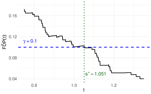
Figure 2: This figure illustrates the construction of $s^{+}$. The smaller the target FDP $\gamma$ is chosen to be, the larger—i.e., stricter—the threshold $s^{+}$ is. In case of directional testing, our method rejects all hypotheses $H_{j}$ with $T_{j}>\delta_{j}+s^{+}$. In case of equivalence testing, it rejects all hypotheses $H_{j}$ with $|T_{j}|<\delta_{j}-s^{+}$.

In simulations, we did not find any setting where Condition 1 was violated. In addition, the following theorem states a property under which Condition 1 is provably satisfied.

Theorem 6.1.

Suppose Assumption 2 holds. Assume that all hypotheses are true or that $(T_{i}:i\in\mathcal{N})$ is independent of $(T_{i}:i\in\mathcal{N}^{c})$, where $\mathcal{N}^{c}=\{1,...,m\}\setminus\mathcal{N}$. Then Condition 1 is satisfied, both in the setting of Section 4.1, i.e. directional testing, and in the setting of Section 5, i.e. equivalence testing. In the former setting, this means that if we reject all hypotheses $H_{j}$ with $T_{j}>\delta_{j}+s^{+}$, then the median of the FDP is at most $\gamma$. In the latter setting, this means that if we reject all hypotheses $H_{j}$ with $|T_{j}|<\delta_{j}-s^{+}$, then the median of the FDP is at most $\gamma$.

A notable property of our methods is that if $\mathcal{R}(0)=\{1,...,m\}$—i.e., all test statistics lie in the noninferiority or equivalence region (e.g. the shaded regions in Figure 1)—then $\tilde{V}(t)=0$ for all $t\geq 0$ and $\mathcal{R}(s^{+})=\{1,...,m\}$. Indeed, if $\mathcal{R}(0)=\{1,...,m\}$, then clearly $\tilde{V}(t)=0$ for all $t\geq 0$ and hence $s=-\infty$, so that $s^{+}=0$ and $\mathcal{R}(s^{+})=\{1,...,m\}$, regardless of $\gamma\in[0,1)$. This property is an extreme example of a more general property of our methods: if $\mathcal{R}(0)$ is large, then the bounds $\tilde{V}(t)$ are small and our mFDP controlling procedure tends to reject many hypotheses. This explains the good simulation results in Sections 7.1 and 7.2.

6.2 Method 2: flexible mFDP control

The method in Hemerik et al. (2024) provides flexible control of the mFDP. This means that the procedure not only ensures that $\mathbb{P}\{FDP>\gamma\}\leq 0.5$ but in addition allows the user to freely choose $\gamma\in[0,1)$ based on the data, without invalidating mFDP control. This added flexibility comes with a price in terms of power. Indeed this procedure is usually less powerful than the method from Section 6.1, as confirmed with simulations in Section 7.2. The flexibility however clearly also has advantages, as discussed in Hemerik et al. (2024).

A seemingly major difference between that method and those that have been proposed in this paper, is that that method is based on $p\text{-values}$, rather than directly using a symmetry property of the test statistics. However, as shown there, it is actually not necessary to have valid $p\text{-values}$, i.e., they need not be uniformly distributed under the null. Moreover, we will show that under Assumption 2, we can transform our test statistics into $p\text{-values}$ that can validly be used within the procedure of Hemerik et al. (2024). In particular, even if we do not known the null distributions of our test statistics $T_{1},...,T_{m}$, then we can simply guess their symmetric null distributions and validly use the resulting invalid $p\text{-values}$ in the method of Hemerik et al. (2024). The reason is that is suffices that the null $p\text{-values}$ stochastically dominate a distribution with a certain symmetry property. Indeed, letting $N=|\mathcal{N}|$, it suffices that the distribution of $(P_{j}:j\in\mathcal{N})$ is stochastically larger than a random vector $(Q_{1},...,Q_{N})$ taking values in $\mathbb{R}^{N}$ that satisfies

$$(Q_{1},...,Q_{N})\,{\buildrel d\over{=}}\,(1-Q_{1},...,1-Q_{N}),$$ (16)

i.e.,

$$(Q_{1}-0.5,...,Q_{N}-0.5)\,{\buildrel d\over{=}}\,(0.5-Q_{1},...,0.5-Q_{N}).$$

The following theorems state that if we construct potentially invalid $p\text{-values}$ in the way just mentioned, then the methods in Hemerik et al. (2024) can be validly applied based on these $p\text{-values}$. Theorem 6.2 is about directional testing and Theorem 6.3 is about equivalence testing.

Theorem 6.2.

Consider the setting of Section 4 (directional testing) and suppose Assumption 2 holds. For every $1\leq j\leq m$, consider some probability density function $f_{j}:\mathbb{R}\rightarrow\mathbb{R}^{+}$ that is symmetric about 0. Here, $f_{j}$ is the guessed or perhaps exactly known null distribution of $T_{j}-\mu_{j}$. For every $1\leq j\leq m$, consider the $p\text{-value}$ $P_{j}=\int_{T_{j}-\delta_{j}}^{\infty}f_{j}(x)dx$.

Then, $(P_{j}:j\in\mathcal{N})$ is deterministically larger than or equal to some vector satisfying property (16). As a consequence the $p\text{-values}$ can validly be used in the methods of Hemerik et al. (2024). In particular, as in Hemerik et al. (2024), let $\mathbb{T}\subset[0,1]$ be the range of $p\text{-value}$ thresholds of interest, where usually a good choice is $\mathbb{T}=[0,0.5]$ or some smaller set. Then the bound $\tilde{B}:\mathbb{T}\rightarrow\mathbb{N}$ constructed in Section 3.3 of that paper satisfies

$$\mathbb{P}\Big{[}\bigcap_{v\in\mathbb{T}}\big{|}\{j\in\mathcal{N}:P_{i}<v\}\big{|}\leq\tilde{B}(v)\Big{]}\geq 0.5,$$

i.e., the values $\tilde{B}(v)/(|\{1\leq j\leq m:P_{i}<v\}\big{|}\vee 1)$ are simultaneous $50\%$ confidence bounds for the number of false positives $|\{j\in\mathcal{N}:P_{i}<v\}|$. In particular, we can choose any $\gamma\in[0,1)$ after seeing the data and choose any rejection threshold $t\in\mathbb{T}$ such that $\tilde{B}(t)/(|\{1\leq j\leq m:P_{i}<t\}\big{|}\vee 1)\leq\gamma$. This will guarantee that the median of the FDP is at most $\gamma$, i.e. $\mathbb{P}(FDP(t)\leq\gamma)\geq 0.5$.

Note that in the theorem, the guessed null distributions $f_{j}$ are not required to be correct, although it can be advantageous power-wise if they are roughly correct. The $p\text{-values}$ from Theorem 6.2 can directly be provided as arguments within the function mFDP.adjust() of the R package mFDP (Hemerik, 2025). This function computes adjused $p\text{-values}$; rejecting the hypotheses with adjusted $p\text{-values}$ smaller than $\gamma$ guarantees that $\mathbb{P}(FDP(t)\leq\gamma)\geq 0.5$.

We now formulate a similar result for the case of equivalence testing.

Theorem 6.3.

Consider the setting of Section 5 (equivalence testing) and suppose Assumption 2 holds. For every $1\leq j\leq m$, consider some probability distribution function $f_{j}:\mathbb{R}\rightarrow\mathbb{R}^{+}$ that is symmetric about 0. Here, $f_{j}$ is the guessed or perhaps exactly known null distribution of $T_{j}-\mu_{j}$. For every $1\leq j\leq m$, define

$$P_{j}=\begin{cases}\int_{T_{j}+\delta_{j}}^{\infty}f_{j}(x)dx&\text{if }T_{j}<0\\ \int_{-\infty}^{T_{j}-\delta_{j}}f_{j}(x)dx&\text{if }T_{j}\geq 0.\end{cases}$$

Then, $(P_{j}:j\in\mathcal{N})$ is larger than or equal to some vector satisfying property (16). As a consequence the results from Theorem 6.2 apply here as well.

7 Simulations and data analysis

In Sections 4-5 we discussed median unbiased estimation of the FDP. The method defined in Section 4.1 is compared to alternatives in Section 7.1 below. Our mFDP controlling method from Section 6.1 is compared with competitors in Section 7.2. Thus, Section 7.1 is about estimation of the FDP and Section 7.2 is about controlling the mFDP, i.e., keeping the mFDP below a prespecified value $\gamma$. Finally, in Section 7.3 we analyze real data.

7.1 Median unbiased estimation of the FDP

The main competitor of our method from Section 4.1 is the SAM procedure from Hemerik and Goeman (2018b), which uses permutations or other transformations to provide a median unbiased estimate of the FDP. Here we will show that for the settings that we are interested in in this paper, i.e. settings with parameters trending in a particular direction, our approach outperforms SAM. For SAM, the transformations that we use below are sign-flips. In case of permutations (of cases and controls), similar results were obtained, i.e. our method clearly outperformed SAM.

To generate test statistics, we first simulated an $n\times m$ matrix of independent standard normal variables, with $n=10$ and $m=500$. In case the data were not normal but had some other symmetric distribution, we obtained comparable results, so here we will stick to normal data. We allowed the test statistics to be correlated, which we achieved by sampling $n$ values and adding the $i$-th value to all elements of the $i$-th row of the data matrix, $1\leq i\leq n$. This leads to a homogeneous correlation structure, where we denote the correlation by $\rho$. To the columns corresponding to the false hypotheses we added a constant $d>0$. The null hypotheses were $H_{j}:\mu_{j}\leq\delta$, $1\leq j\leq m$, where $\delta:=0$.

In Figure 3 the average estimate $\tilde{FDP}$ of our method is compared to SAM’s median unbiased estimate. Here $\pi_{0}:=|\mathcal{N}|/m$ is the number of true hypotheses divided by the total number of hypotheses. It can be seen that our method provided on average lower estimates of the FDP when there were many false hypotheses, which is the situation we are interested in in this paper.

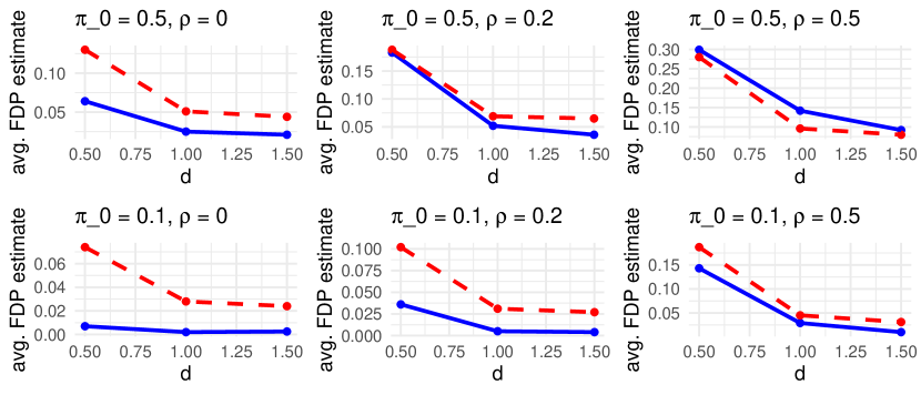
Figure 3: The average FDP estimate of our novel estimator $\tilde{FDP}$ from Section 4 (solid lines) and SAM (dashed lines) as depending on the fraction $\pi_{0}$ of true hypotheses, the homogeneous correlation $\rho$ between the test statistics and the effect size $d$. The number of hypotheses was $m=500$. Each estimate is based on $5\cdot 10^{3}$ simulations.

As discussed in Section 2.2, SAM is uniformly improved by SAM+CT. However, SAM+CT is only computationally feasible when $m$ is not too large. Hence we took $m=50$ in the simulations of SAM+CT. A comparison of the novel method, SAM and SAM+CT is in Figure 4. Note that SAM+CT clearly performed better than SAM. Further, we see that our method performed relatively well when $\pi_{0}$ was small, which is the setting we are interested in here. The additional advantage of our method is that it is very fast, unlike SAM+CT, which is computationally infeasible for large problems.

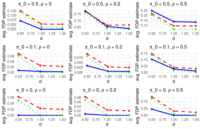
Figure 4: The average FDP estimate of our novel estimator $\tilde{FDP}$ from Section 4 (solid lines), SAM (dashed) and SAM+CT (dotted) as depending on the fraction $\pi_{0}$ of true hypotheses, the correlation $\rho$ between the test statistics and the effect size $d$. The number of hypotheses was taken to be $m=50$, since SAM+CT is computationally infeasible for large $m$. Each estimate is based on $10^{3}$ simulations.

7.2 mFDP control

Here, we show that the novel mFDP controlling procedure from Section 6.1 often has better power than some major competitors. The first method that we compare with, is the procedure from Hemerik et al. (2024) discussed in Section 6.2. This method is implemented in the function mFDP.adjust from the R package mFDP (Hemerik, 2025). It is relevant to mention that that method is already compared with the procedures from Goeman et al. (2019) and Katsevich and Ramdas (2020) in simulations in Hemerik et al. (2024).

In addition, we compare with the adaptive version of the Lehmann-Romano method (Lehmann and Romano, 2005; Döhler and Roquain, 2020), which is implemented in the R package FDX (Dohler et al., 2024). This method provides FDX control; we set the confidence level to 0.5, so that the method controlled the mFDP.

Further, we compare with the Benjamini-Hochberg procedure, which controls the mean rather than the median of the FDP (Benjamini and Hochberg, 1995). The Benjamini-Hochberg method is based on $p\text{-values}$. The $p\text{-values}$ used by Lehmann-Romano and Benjamini-Hochberg were right-sided and were computed by comparing the test statistics with the standard normal distribution.

The data were simulated as in Section 7.1. For each method, the target $FDP$, $\gamma$—often called $\alpha$ in the context of Benjamini-Hochberg—was set to 0.1. We computed the power as the mean fraction of false hypotheses that were rejected. We considered effect sizes $d\in\{1,2,3\}$. Again, we focused on settings where $\pi_{0}$ was far from 1, which are the settings we are interested in in this paper. The results are in Figure 5. We see that our method had better power than the other methods, although naturally the difference with the method from Hemerik et al. (2024) was small when that method had power near $100\%$.

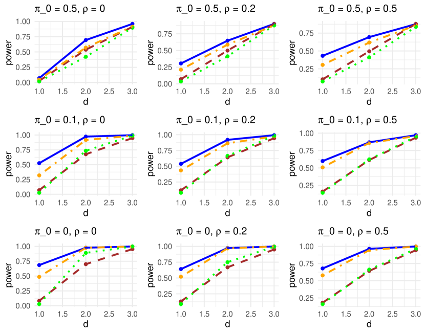
Figure 5: The power of our novel method from Section 6.1 (solid lines) versus Benjamini-Hochberg (dashed), Lehmann-Romano (dotted) and the method from Hemerik et al. (2024) (dash-dotted) as depending on the fraction $\pi_{0}$ of true hypotheses, the correlation $\rho$ between the test statistics and the effect size $d$. The number of hypotheses was $m=500$. Each estimate is based on $5\cdot 10^{3}$ simulations.

7.3 Data analysis

To illustrate the methodology, we applied it to the gene expression data that were considered in Tusher et al. (2001) and Hemerik and Goeman (2018b). The dataset contains gene expression levels of $m=7129$ genes. For each gene there are eight observations, four of which are from irradiated cells and four from unirradiated cells. In the mentioned papers, the goal was to find genes that were differentially expressed between the two groups. Here, we will consider a different goal, namely equivalence testing.

For each $1\leq j\leq m$ we computed the Welch t-statistic $T_{j}$ corrresponding to the $j$-th gene. Note that one usually assumes that the data are normal, but this is not required for our methodology. For each $1\leq j\leq m$ we considered the null hypothesis $H_{j}:|\mu_{j}|\geq\delta:=2$, where $\mu_{j}=\mathbb{E}(T_{j})$.

We first applied the method from Section 5, which rejects the hypotheses in $\mathcal{R}(t)=\{1\leq j\leq m:|T_{j}|<\delta-t\}$ and provides a median unbiased estimate $\tilde{V}(t)$ of the number of false positives $V(t)$. For $t=1$, we found $R(t)=5134$, where we recall that $R=|\mathcal{R}|$. The estimate $\tilde{V}(t)$ was 111. Thus, a median unbiased estimate of the FDP was $\tilde{V}(t)/R(t)\approx 0.022.$ Note that we cannot compare our estimate with SAM, since SAM does not allow for equivalence testing.

Often we do not want to estimate the FDP for a given threshold $t$, but wish to reject a set of hypotheses in such a way that the mFDP is below some pre-specified target value $\gamma$. Hence, we applied the mFDP controlling procedure from Section 6.1, to test the hypotheses of non-equivalence $H_{j}:|\mu_{j}|\geq 2$ with target FDP $\gamma=0.05$. The procedure resulted in the rejection threshold $s^{+}=0.0957...\approx 0.096.$ We obtained $R(s^{+})=6660$, i.e., we can reject 6660 hypotheses. In other words, if we reject the 6660 hypotheses with the test statistics closest to 0, then the median of the FDP is at most $\gamma=0.05$. When we increased $\gamma$ to $0.1$, we rejected $6733$ hypotheses.

8 Discussion

In many multiple testing problems, test statistics are symmetric about their means $\mu_{j}$. In this paper, we have taken this property as our main assumption. If we expect a priori that most of the $\mu_{j}$ lie in the directions or intervals corresponding to the alternative hypotheses, then our procedures exploit this effectively and gain power compared to existing methods. At the same time, our methods are valid for finite samples, regardless of whether these a priori expectations are correct.

Because of their combinatorical nature, nonparametric approaches such as ours lend themselves better to controlling the median of the FDP (Romano and Wolf, 2007; Hemerik and Goeman, 2018b; Hemerik et al., 2019) than to controlling the mean of the FDP, i.e., the FDR. However, FDR control is definitely an attractive criterion. For example, FDR control always implies weak FWER control. This means that if all hypotheses are true, then the probability of at least one incorrect rejection will be controlled. On the other hand, in the settings that we are interested here, most hypotheses tend to be false, so weak FWER control is less of an advantage here. Besides, we could guarantee weak FWER control as well by first performing a global test, which tests whether all $m$ hypotheses are true. Another relevant point though is that the distribution of the FDP tends to be skewed to the right, so that naturally the mFDP tends to be smaller than the FDR. In conclusion, we feel that mFDP control should only be preferred over FDR control when there are specific reasons for this, such as the availability of an mFDP method with much better power or with fewer assumptions. For example, in the settings that we are interested in in this paper, FDR methods with proven finite-sample validity tend to be very conservative, which can be a reason to use our mFDP approach instead.

The way in which we estimate the FDP based on a symmetry property is related to the knockoffs procedures from Barber and Candès (2015). In many respects those methods are very different and the underlying setting is different. However, the similarity is that the knockoffs procedures are also based on counting how many test statistics are above $t$ and below $-t$, for different $t\geq 0$. A difference between their approach and ours is that test statistics based on knockoffs are mutually independent, whereas here they are potentially dependent.

Our multiple testing approach is clearly nonparametric, since it requires no assumptions about the distributional shapes of the test statistics, except symmetry. What makes our methods different from other nonparametric procedures—e.g. permutation methods such as Hemerik and Goeman (2018b), Hemerik et al. (2019) and Blain et al. (2022)—is that we do not directly use symmetries of the data, but only of the resulting test statistics. This would seem very crude, and e.g. using permutations—if possible—would seem more sophisticated. However, when most of the hypotheses are false, our approach tends to lead to very low bounds for $V$ and consequently high power, as explained conceptually in Section 6.1. Thus, our approach is very adaptive, in the sense that it adapts very well to the amount of signal in the data. Additionally, when implemented with care, all methods in this paper have a computation time that is linear in $m$, after sorting the test statistics. All in all, the proposed methods combine multiple attractive properties: they do not require independence and are exact, very adaptive and fast.

Future work might relax some of the assumptions in this paper, e.g. those in Theorem 6.1 and in Section C from the Supplement. In addition, there are open problems regarding FDX control with $\alpha<0.5$ in nonparametric settings, as discussed at the beginning of Section 6.1. Finally, it is likely that in fields such as food safety evaluation (Vahl and Kang, 2017; Leday et al., 2023), multiple testing problems of the kind we have focused on will become more frequent, which may inspire further research related to ours.

Appendix A Proofs of results

A.1 Proof of Theorem 2.1

Proof.

The statements about the case $\theta=0$ follow directly from the general group invariance testing principle, see e.g. Hoeffding (1952), Lehmann and Romano (2022, Theorem 17.2.1) and Hemerik and Goeman (2018a). Now suppose $\theta<0$. Let $\theta_{n}$ denote the $n$-vector $(\theta,...,\theta)^{\prime}$. Define $X^{*}=X-\theta_{n}$. The entries of $X^{*}$ are symmetric with mean $0$ and hence

$$\mathbb{P}(T_{id}(X^{*})>T^{(1-\alpha)}(X^{*}))\leq\alpha$$ (17)

by e.g. Hemerik and Goeman (2018a). Now note that

$$T_{id}(X^{*})=T_{id}(X)-n^{-1/2}n\theta,$$ (18)

where $-n^{-1/2}n\theta$ is positive. Further, for any transformation $g\in\mathcal{G}$ we have

$$T_{g}(X^{*})\leq T_{g}(X)-n^{-1/2}n\theta$$

The latter implies that

$$T^{(1-\alpha)}(X^{*})\leq T^{(1-\alpha)}(X)-n^{-1/2}n\theta.$$ (19)

From expressions (18) and (19) and the fact that $-n^{-1/2}n\theta>0$, it follows that the following implication always holds:

$$T_{id}(X)>T^{(1-\alpha)}(X)\implies T_{id}(X^{*})>T^{(1-\alpha)}(X^{*}).$$

Hence,

$$\mathbb{P}\Big{\{}\text{reject }H_{0}\Big{\}}=\mathbb{P}\Big{\{}T_{id}(X)>T^{(1-\alpha)}(X)\Big{\}}\leq\mathbb{P}\Big{\{}T_{id}(X^{*})>T^{(1-\alpha)}(X^{*})\Big{\}}\leq\alpha.$$

by inequality (17). This finishes the proof. ∎

A.2 Proof of Theorem 2.2

Proof.

In the literature it is quite common to consider the point null hypothesis $H_{0}:\theta=0$. As remarked, in that case the results directly follow from e.g. Hemerik and Goeman (2018a). Now suppose $\theta<0$. We define $X^{*}=\{(Z-\theta^{1}_{n})^{\prime},(Y-\theta^{2}_{n})^{\prime}\}^{\prime}$, where $\theta^{1}_{n}$ and $\theta^{2}_{n}$ denote the $n$-vectors $(\theta^{1},...,\theta^{1})^{\prime}$ and $(\theta^{2},...,\theta^{2})^{\prime}$ respectively. Then the distribution of $X^{*}$ is permutation-invariant, so that by e.g. Hemerik and Goeman (2018a),

$$\mathbb{P}_{H_{0}}(T_{id}(X^{*})>T^{(1-\alpha)}(X^{*}))\leq\alpha.$$

Now note that

$$T_{id}(X^{*})=T_{id}(X)-n^{-1/2}(n\theta^{1}-n\theta^{2}),$$ (20)

where $-n^{-1/2}(n\theta^{1}-n\theta^{2})>0$ , since $\theta^{1}-\theta^{2}=\theta<0$. Further, for any transformation $g\in\mathcal{G}$ we have

$$T_{g}(X^{*})\leq T_{g}(X)-n^{-1/2}(n\theta^{1}-n\theta^{2}).$$

The latter implies that

$$T^{(1-\alpha)}(X^{*})\leq T^{(1-\alpha)}(X)-n^{-1/2}(n\theta^{1}-n\theta^{2}).$$ (21)

From results (20) and (21) it follows that the following implication always holds:

$$T_{id}(X)>T^{(1-\alpha)}(X)\implies T_{id}(X^{*})>T^{(1-\alpha)}(X^{*}).$$

The result now follows as at the end of the proof of Theorem 2.1.

∎

A.3 Proof of Theorem 4.1

Proof.

We have $V(t)=$

$$|\{j\in\mathcal{N}:T_{j}>\delta_{j}+t\}|\leq$$

$$|\{j\in\mathcal{N}:T_{j}>\mu_{j}+t\}|=$$

$$|\{j\in\mathcal{N}:T_{j}-\mu_{j}>t\}|=:N_{1},$$

where we used that if $j\in\mathcal{N}$, then $\delta_{j}\geq\mu_{j}$.

Note that

$$R^{-}(t)=|\{1\leq j\leq m:T_{j}<\delta_{j}-t\}|\geq$$

$$|\{j\in\mathcal{N}:T_{j}<\delta_{j}-t\}|\geq$$

$$|\{j\in\mathcal{N}:T_{j}-\mu_{j}<-t\}|=:N_{2},$$

where we again used that if $j\in\mathcal{N}$ then $\delta_{j}\geq\mu_{j}$.

Thus, $V(t)\leq N_{1}$ and $R^{-}\geq N_{2}$. Consequently,

$$\mathbb{P}\{V(t)\leq R^{-}(t)\}\geq\mathbb{P}\{N_{1}\leq N_{2}\}=$$

$$\mathbb{P}\Big{\{}|j\in\mathcal{N}:T_{j}-\mu_{j}>t\}|\leq|\{j\in\mathcal{N}:T_{j}-\mu_{j}<-t\}|\Big{\}}$$

By Assumption 2, the above equals

$$\mathbb{P}\Big{\{}|j\in\mathcal{N}:-(T_{j}-\mu_{j})>t\}|\leq|\{j\in\mathcal{N}:-(T_{j}-\mu_{j})<-t\}|\Big{\}}$$

$$\mathbb{P}\Big{\{}|i\in\mathcal{N}:T_{j}-\mu_{j}<-t\}|\leq|\{i\in\mathcal{N}:T_{j}-\mu_{j}>t\}|\Big{\}}$$

but this is exactly $\mathbb{P}\{N_{2}\leq N_{1}\}$. Thus $\mathbb{P}(N_{1}\leq N_{2})=\mathbb{P}(N_{2}\leq N_{1})$. Since the sum of these probabilities is at least 1, It follows that $\mathbb{P}(N_{1}\leq N_{2})\geq 0.5$.

Note that since $V(t)\leq R(t)$, we have

$$V(t)\leq\tilde{V}(t)\quad\Leftrightarrow\quad V(t)\leq R^{-}(t)\wedge R(t)\quad\Leftrightarrow\quad V(t)\leq R^{-}(t).$$

Thus,

$$\mathbb{P}\big{\{}V(t)\leq\tilde{V}(t)\big{\}}=\mathbb{P}\big{\{}V(t)\leq R^{-}(t)\big{\}}\geq\mathbb{P}\big{\{}N_{1}\leq N_{2}\big{\}}\geq 0.5.$$

Note that $V(t)\leq\tilde{V}(t)$ implies $FDP(t)\leq\tilde{FDP}(t)$, so that we also have

$$\mathbb{P}(FDP(t)\leq\tilde{FDP}(t))\geq 0.5.$$

∎

A.4 Proof of Lemma 4.2

Proof.

We have

$$V(t)=|\{j\in\mathcal{N}:T_{j}>\delta_{j}+t\}|=$$

$$|\{j\in\mathcal{N}:T_{j}-\mu_{j}>t\}|$$

and

$$R^{-}(t)=|\{1\leq j\leq m:T_{j}<\delta_{j}-t\}|=$$

$$|\{j\in\mathcal{N}:T_{j}<\delta_{j}-t\}|=$$

$$|\{j\in\mathcal{N}:T_{j}-\mu_{j}<-t\}|.$$

Thus,

$$\mathbb{P}\{V(t)\leq R^{-}(t)\}=$$

$$\mathbb{P}\{|\{j\in\mathcal{N}:T_{j}-\mu_{j}>t\}|\leq|\{j\in\mathcal{N}:T_{j}-\mu_{j}<-t\}|\}.$$

We now reason analogously to the proof of Theorem 4.1. By Assumption 2, the above equals

$$\mathbb{P}\{|\{j\in\mathcal{N}:-(T_{j}-\mu_{j})>t\}|\leq|\{j\in\mathcal{N}:-(T_{j}-\mu_{j})<-t\}|\}=$$

$$\mathbb{P}\Big{\{}|i\in\mathcal{N}:T_{j}-\mu_{j}<-t\}|\leq|\{i\in\mathcal{N}:T_{j}-\mu_{j}>t\}|\Big{\}}$$

but this is exactly $\mathbb{P}\{R^{-}(t)\leq V(t)\}$. Hence, $\mathbb{P}\{V(t)\leq R^{-}(t)\}=\mathbb{P}\{V(t)\leq R^{-}(t)\}$, which means that these probabilities are at least $0.5$. Note that $\mathbb{P}(E_{1})+\mathbb{P}(E_{2})+\mathbb{P}(E_{3})=1$ and $\mathbb{P}(E_{1})=\mathbb{P}(E_{3}).$ Thus, $2\mathbb{P}(E_{1})+\mathbb{P}(E_{2})=1$, so that $\mathbb{P}(E_{1})=0.5-0.5\mathbb{P}(E_{2}))$. ∎

A.5 Proof of Proposition 4.3

Proof.

Proof of first statement. Define the random variables $N_{1}$ and $N_{2}$ as in the proof of Theorem 4.1:

$$N_{1}=|\{j\in\mathcal{N}:T_{j}-\mu_{j}>t\}|,$$

$$N_{2}=|\{j\in\mathcal{N}:T_{j}-\mu_{j}<-t\}|.$$

We have

$$\mathbb{P}\{V(t)\leq\tilde{V}^{\prime}(t)|R(t)\neq R^{-}(t)\}=$$

$$\mathbb{P}\{V(t)\leq\tilde{V}(t)|R(t)\neq R^{-}(t)\}=$$

$$\mathbb{P}\{V(t)\leq R^{-}(t)|R(t)\neq R^{-}(t)\}.$$

As in the proof of Theorem 4.1, we have $V(t)\leq N_{1}$ and $R^{-}(t)\geq N_{2}$. Hence the above is at least

$$\mathbb{P}\{N_{1}\leq N_{2}|R(t)\neq R^{-}(t)\}=$$

$$\mathbb{P}\{N_{2}\leq N_{1}|R(t)\neq R^{-}(t)\}\geq$$

$$\mathbb{P}\{R^{-}(t)\leq V(t)|R(t)\neq R^{-}(t)\}.$$

Since

$$\mathbb{P}\{V(t)\leq R^{-}(t)|R(t)\neq R^{-}(t)\}+\mathbb{P}\{R^{-}(t)\leq V(t)|R(t)\neq R^{-}(t)\}\geq 1,$$

it follows that

$$\mathbb{P}\{V(t)\leq R^{-}(t)|R(t)\neq R^{-}(t)\}\geq 0.5$$

and hence

$$\mathbb{P}\{V(t)\leq\tilde{V}^{\prime}(t)|R(t)\neq R^{-}(t)\}\geq 0.5.$$

Further,

$$\mathbb{P}\{V(t)\leq\tilde{V}^{\prime}(t)|R(t)=R^{-}(t)\}=\mathbb{P}\{d=1|R(t)=R^{-}(t)\}=0.5.$$

From the law of total probability it follows that $\mathbb{P}\{V(t)\leq\tilde{V}^{\prime}(t)\}\geq 0.5.$

Proof of second statement. Suppose that for all $1\leq j\leq m$ we have $\mu_{j}=\delta$. Then $V(t)=R(t)$. Define $E_{1}$, $E_{2}$ and $E_{3}$ as in Lemma 4.2. Note that

$$\mathbb{P}\{V(t)>\tilde{V}^{\prime}(t)\}=$$

$$\mathbb{P}\Big{\{}V(t)>\tilde{V}^{\prime}(t)\text{ and }V(t)\neq R^{-}(t)\Big{\}}+\mathbb{P}\Big{\{}V(t)>\tilde{V}^{\prime}(t)\text{ and }V(t)=R^{-}(t)\Big{\}}.$$

Since $R(t)=V(t)$, the above equals

$$\mathbb{P}\Big{\{}V(t)>\tilde{V}^{\prime}(t)\text{ and }R(t)\neq R^{-}(t)\Big{\}}+\mathbb{P}\Big{\{}V(t)>\tilde{V}^{\prime}(t)\text{ and }R(t)=R^{-}(t)\Big{\}}=$$

$$\mathbb{P}\Big{\{}V(t)>\tilde{V}(t)\text{ and }R(t)\neq R^{-}(t)\Big{\}}+\mathbb{P}\Big{\{}R(t)=R^{-}(t)\text{ and }d=-\infty\Big{\}}=$$

$$\mathbb{P}\Big{\{}V(t)>R^{-}(t)\text{ and }R(t)\neq R^{-}(t)\Big{\}}+0.5\mathbb{P}\{R(t)=R^{-}(t)\}=$$

$$\mathbb{P}\{V(t)>R^{-}(t)\}+0.5\mathbb{P}\{V(t)=R^{-}(t)\},$$ (22)

where we used that $V(t)=R(t)$. Recall that $\{V(t)>R^{-}(t)\}=E_{3}$ and $\mathbb{P}\{V(t)=R^{-}(t)\}=E_{2}.$

Now, by Lemma 4.2 we have $\mathbb{P}(E_{1})=\mathbb{P}(E_{3})$, so that $\mathbb{P}(E_{3})=0.5\mathbb{P}(E_{1})+0.5\mathbb{P}(E_{3})$. Thus, expression (22) equals

$$\mathbb{P}(E_{3})+0.5\mathbb{P}(E_{2})=$$

$$0.5\mathbb{P}(E_{1})+0.5\mathbb{P}(E_{3})+0.5\mathbb{P}(E_{2})=$$

$$0.5(\mathbb{P}(E_{1})+\mathbb{P}(E_{2})+\mathbb{P}(E_{3}))=0.5\cdot 1=0.5,$$

as was to be shown.

∎

A.6 Proof of Proposition 4.4

Proof.

For any true intersection hypothesis $H_{I}$ with $I\in\mathcal{C}$,

$$\mathbb{P}(\tilde{\phi}_{I}=1)=\mathbb{P}(R_{I}>R^{-}_{I})=$$

$$\mathbb{P}\Big{(}|\{j\in I:T_{j}>\delta_{j}+t\}|>|\{j\in I:T_{j}<\delta_{j}-t\}|\Big{)}.$$

Note that for every $j\in I$, $\mu_{j}\leq\delta_{j}$, since $H_{i}$ is true. Hence the above is at most

$$\mathbb{P}\Big{(}|\{j\in I:T_{j}-\mu_{j}>t\}|>|\{j\in I:T_{j}-\mu_{j}<-t\}|\Big{)}.$$

Similarly to other proofs, by symmetry of $(T_{j}-\mu_{j}:j\in I)$ the above is at most $0.5=\alpha$. This finishes the proof. ∎

A.7 Proof of Proposition 4.5

Proof.

For $I\in\mathcal{C}$ we have

$$I\in\mathcal{X}\Leftrightarrow$$

$$\tilde{\phi}_{J}=1\text{ for all }I\subseteq J\subseteq\mathcal{C}\Leftrightarrow$$

$$R_{J}>R^{-}_{J}\text{ for all }I\subseteq J\subseteq\mathcal{C}\Leftrightarrow$$

$$|\{j\in J:T_{j}>\delta_{j}+t\}|>|\{j\in J:T_{j}<\delta_{j}-t\}|\text{ for all }I\subseteq J\subseteq\mathcal{C}\Leftrightarrow$$

$$|\{i\in I:T_{j}>\delta_{j}+t\}|>|\{j\in\{1,...,m\}:T_{j}<\delta_{j}-t\}|\Leftrightarrow$$

$$R_{I}>R^{-}.$$

Thus, $I\in\mathcal{X}$ if and only if $R_{I}>R^{-}$. ∎

A.8 Proof of Lemma 4.6

Proof.

Let $I\in\mathcal{C}$. We must give an example of a distribution of $(T_{1},...,T_{m})$ satisfying Assumption 2 for which $\mathbb{P}(\delta^{\prime}_{I}=1)=0.5$. In fact, it holds for any distribution that satisfies Assumption 2 and in addition satisfies $\mu_{j}=\delta_{j}$ for all $1\leq j\leq m$. Indeed, then $(T_{j}-\delta_{j}:j\in I)\,{\buildrel d\over{=}}\,-(T_{j}-\delta_{j}:j\in I)$ and hence $\mathbb{P}(R_{I}(t)>R_{I}^{-}(t))=\mathbb{P}(R_{I}(t)<R_{I}^{-}(t))$. Further, $\mathbb{P}(b=1)=0.5$. Consequently, $\mathbb{P}(\tilde{\phi}^{\prime}_{I}=1)=0.5$. ∎

A.9 Proof of Lemma 4.7

Proof.

Suppose such a $\phi^{*}_{I}$ exists and pick one. Since $\mathbb{P}(\phi^{*}_{I}>\tilde{\phi}^{\prime}_{I})>0$, we can choose a subset $A\subset\mathbb{R}^{n}$ with strictly positive Lebesgue measure such that if $(t_{1},...,t_{m})\in A$, then $\phi^{*}_{I}((t_{1},...,t_{m}))=1$ and $\tilde{\phi}^{\prime}_{I}((t_{1},...,t_{m}))=0$. Since the support of $(T_{1},...,T_{m})$ is generally $\mathbb{R}^{m}$, it follows that generally $\mathbb{P}(\tilde{\phi}^{\prime}_{I}=1)<\mathbb{P}(\phi^{*}_{I}=1)$, so that if $H_{I}$ is true, then $\mathbb{P}(\tilde{\phi}^{\prime}_{I}=1)<0.5$ . However, by Lemma 4.6 this cannot generally hold. Thus, there is no such test $\phi^{*}_{I}$, as was to be shown. ∎

A.10 Proof of Proposition 4.8

Proof.

Let $I\in\mathcal{C}$. Note that for $J\subseteq\mathcal{C}$, $\tilde{\phi}_{J}^{\prime}=1$ means that either $R_{J}>R^{-}_{J}$ or $\{R_{J}=R^{-}_{J}\}\cap\{b=1\}$ holds. Suppose that $b=1$. Then $\tilde{\phi}_{J}=1$ if and only if $R_{J}\geq R^{-}_{J}$. Hence, then

$$I\in\mathcal{X}\Leftrightarrow$$

$$R_{J}\geq R^{-}_{J}\text{ for all }I\subseteq J\subseteq\mathcal{C}\Leftrightarrow$$

$$\big{|}\big{\{}j\in J:T_{j}>\delta_{j}+t\big{\}}\big{|}\geq\big{|}\big{\{}j\in J:T_{j}<\delta_{j}-t\big{\}}\big{|}\text{ for all }I\subseteq J\subseteq\mathcal{C}\Leftrightarrow$$

$$\big{|}\big{\{}j\in I:T_{j}>\delta_{j}+t\big{\}}\big{|}\geq\big{|}\big{\{}j\in\{1,...,m\}:T_{j}<\delta_{j}-t\big{\}}\big{|}\Leftrightarrow$$

$$R_{I}\geq R^{-}.$$

Now suppose that $b=0$. Then it analogously follows that $I\in\mathcal{X}\Leftrightarrow R_{I}>R^{-}$.

We see that in general $\mathbbm{1}(I\in\mathcal{X})=\mathbbm{1}(R_{I}>R^{-})+b\mathbbm{1}(R_{I}=R^{-})$. Consider the following events, whose union has probability 1.

• Event 1: $R_{I}=R_{I}^{-}$ and $b=1$. Then $\tilde{V}^{\prime}=d=-\infty<R_{I}$.

• Event 2: $R_{I}>R^{-}$. Then $R^{-}<R_{I}\leq R$ and hence $\tilde{V}^{\prime}=R\wedge R^{-}=R^{-}<R_{I}$.

• Event 3: $R_{I}<R^{-}$ and $\{R_{I}\neq R_{I}^{-}\}\cup\{b=0\}$ and $R\leq R^{-}$. Then $\tilde{V}^{\prime}=R\wedge R^{-}=R\geq R_{I}$.

• Event 4: $R_{I}<R^{-}$ and $\{R_{I}\neq R_{I}^{-}\}\cup\{b=0\}$ and $R>R^{-}$. Then $\tilde{V}^{\prime}=R\wedge R^{-}=R^{-}>R_{I}.$

• Event 5: $R_{I}=R^{-}$ and $\{R_{I}\neq R_{I}^{-}\}\cup\{b=0\}$. Then $\tilde{V}^{\prime}=\tilde{V}=R\wedge R^{-}=R^{-}=R_{I}$.

Consequently, $R_{I}>\tilde{V^{\prime}}$ if and only if event 1 or 2 happens. We conclude that

$$\mathbbm{1}(I\in\mathcal{X})=\mathbbm{1}(R_{I}>R^{-})+b\mathbbm{1}(R_{I}=R^{-})=\mathbbm{1}(R_{I}>\tilde{V^{\prime}}),$$

so that we are done.

∎

A.11 Proof of Theorem 4.9

Proof.

As already shown in the main text, the closed testing procedure based on the local tests $\tilde{\phi}^{\prime}_{I}$, $I\in\mathcal{C}$, is admissible in the sense of Goeman et al. (2021). Now suppose $\tilde{V}^{\prime}$ is not admissible. Choose a procedure producing bounds $\tilde{V}^{*}(t)$ with the three mentioned properties stated in the theorem. Further, pick a distribution satisfying Assumption 2 such that $\mathbb{P}\{\tilde{V}^{\prime}(t)>\tilde{V}^{*}(t)\}>0$. We discussed in the main text that $\tilde{V}^{\prime}(t)$ is equivalent to an admissible closed testing procedure, namely the procedure that provides the upper bound $|I|\wedge(|I\cap\mathcal{R}^{c}|+\tilde{V}^{\prime})$ for every $I\subseteq\mathcal{C}$. Note that $\tilde{V}^{*}(t)$ is equivalent to a procedure that is uniformly better, namely the procedure that provides the upper bound $|I|\wedge(|I\cap\mathcal{R}^{c}|+\tilde{V}^{*})$ for every $I\subseteq\mathcal{C}$. This is a contradiction with the admissibility of the former procedure. This finishes the proof. ∎

A.12 Proof of Theorem 5.1

Proof.

Write

$$\mathcal{N}^{-}= \{j\in\mathcal{N}:\mu_{j}\leq-\delta_{j}\},$$

$$\mathcal{N}^{+}= \{j\in\mathcal{N}:\mu_{j}\geq\delta_{j}\}.$$

Note that $\mathcal{N}=\mathcal{N}^{-}\cup\mathcal{N}^{+}$.

We have $V(t)=$

$$|j\in\mathcal{N}:|T_{j}|<\delta_{j}-t\}|=$$

$$\Big{|}\{j\in\mathcal{N}^{-}:|T_{j}|<\delta_{j}-t\}\cup\{j\in\mathcal{N}^{+}:|T_{j}|<\delta_{j}-t\}\Big{|}\leq$$

$$\Big{|}\{j\in\mathcal{N}^{-}:T_{j}>-(\delta_{j}-t)\}\cup\{j\in\mathcal{N}^{+}:T_{j}<\delta_{j}-t\}\Big{|}\leq$$

$$\Big{|}\{j\in\mathcal{N}^{-}:T_{j}-\mu_{j}>t\}\cup\{j\in\mathcal{N}^{+}:T_{j}-\mu_{j}<-t\}\Big{|}=:Z_{1},$$

where the last step follows from the fact that if $j\in\mathcal{N}^{-}$, then $\mu_{j}\leq-\delta_{j}$ so $-\mu_{j}\geq\delta_{j}$, and if $j\in\mathcal{N}^{+}$, then $\mu_{j}\geq\delta_{j}$ so $-\mu_{j}\leq-\delta_{j}$.

We have $\tilde{V}(t)=$

$$|\{1\leq j\leq m:|T_{j}|>\delta_{j}+t\}|\geq$$

$$|\{j\in\mathcal{N}:|T_{j}|\geq\delta_{j}+t\}|=$$

$$\Big{|}\{i\in\mathcal{N}:T_{j}<-\delta_{j}-t\}\cup\{j\in\mathcal{N}:T_{j}>\delta_{j}+t\}\Big{|}\geq$$

$$\Big{|}\{i\in\mathcal{N}^{-}:T_{j}<-\delta_{j}-t\}\cup\{j\in\mathcal{N}^{+}:T_{j}>\delta_{j}+t\}\Big{|}\geq$$

$$\Big{|}\{i\in\mathcal{N}^{-}:T_{j}-\mu_{j}<-t\}\cup\{j\in\mathcal{N}^{+}:T_{j}-\mu_{j}>t\}\Big{|}=:Z_{2},$$

where the last inequality follows from the fact that if $j\in\mathcal{N}^{-}$ then $\mu_{j}\leq-\delta_{j}$ so $-\mu_{j}\geq\delta_{j}$ and if $j\in\mathcal{N}^{+}$ then $\mu_{j}\geq\delta_{j}$ so $-\mu_{j}\leq-\delta_{j}$.

We consequently have $\mathbb{P}(V(t)\leq\tilde{V}(t))\geq\mathbb{P}(Z_{1}\leq Z_{2})$=

$$\mathbb{P}\Big{\{}\big{|}\{j\in\mathcal{N}^{-}:T_{j}-\mu_{j}>t\}\cup\{i\in\mathcal{N}^{+}:T_{j}-\mu_{j}<-t\}\big{|}\leq$$

$$\big{|}\{i\in\mathcal{N}^{-}:T_{j}-\mu_{j}<-t\}\cup\{j\in\mathcal{N}^{+}:T_{j}-\mu_{j}>t\}\big{|}\Big{\}}.$$

By Assumption 2, the above equals

$$\mathbb{P}\Big{\{}|\{j\in\mathcal{N}^{-}:T_{j}-\mu_{j}<-t\}\cup\{i\in\mathcal{N}^{+}:T_{j}-\mu_{j}>t\}|\leq$$

$$|\{j\in\mathcal{N}^{-}:T_{j}-\mu_{j}>t\}\cup\{j\in\mathcal{N}^{+}:T_{j}-\mu_{j}<-t\}|\Big{\}},$$

but this is $\mathbb{P}(Z_{2}\leq Z_{1})$. Thus $\mathbb{P}(Z_{1}\leq Z_{2})=\mathbb{P}(Z_{2}\leq Z_{1})$. Since the sum of these probabilities is at least 1, It follows that $\mathbb{P}(Z_{1}\leq Z_{2})\geq 0.5$. Consequently, $\mathbb{P}(V(t)\leq\tilde{V}(t))\geq 0.5$, as was to be shown. ∎

A.13 Proof of Proposition 5.2

Proof.

For $I\in\mathcal{C}$ we have

$$I\in\mathcal{X}\Leftrightarrow$$

$$\tilde{\phi}^{\prime}_{J}=1\text{ for all }I\subseteq J\subseteq\mathcal{C}\Leftrightarrow$$

$$R_{J}>R^{-}_{J}\text{ for all }I\subseteq J\subseteq\mathcal{C}\Leftrightarrow$$

$$|\{j\in J:|T_{j}|<\delta_{j}-t\}|>|\{j\in J:|T_{j}|>\delta_{j}+t\}|\text{ for all }I\subseteq J\subseteq\mathcal{C}.$$

Note that the above holds if and only if $R_{I}>R^{-}$. Thus, $I\in\mathcal{X}$ if and only if $R_{I}>R^{-}$. ∎

A.14 Proof of Theorem 6.1

Proof.

We first provide a proof for the case of one-sided testing (Section 4.1). We then give the proof for the case of equivalence testing (Section 5), which is analogous.

Proof for the case of one-sided testing
We first define some quantities. Then we give an overview of the three steps of the proof. Finally, we prove the three steps in detail. For $t\geq 0$, let

$$A^{-}(t)=|\{j\in\mathcal{N}^{c}:T_{j}<\delta_{j}-t\}|,$$

$$A^{+}(t)=|\{j\in\mathcal{N}^{c}:T_{j}>\delta_{j}+t\}|,$$

$$N^{-}(t)=|\{j\in\mathcal{N}:T_{j}<\delta_{j}-t\}|,$$

$$N^{+}(t)=|\{j\in\mathcal{N}:T_{j}>\delta_{j}+t\}|,$$

where in fact $N^{+}=V$. Further, note that $R=N^{+}+A^{+}$ and $R^{-}=N^{-}+A^{-}$. Observe that

$$FDP=\frac{N^{+}}{(N^{+}+A^{+})\vee 1}.$$

Define

$$\tilde{FDP}^{*}:=\frac{N^{-}}{(N^{+}+A^{+})\vee 1}\wedge 1\leq\frac{N^{-}+A^{-}}{(N^{+}+A^{+})\vee 1}\wedge 1=\tilde{FDP}.$$

Note that

$$FDP>\gamma\Leftrightarrow N^{+}>\gamma({N^{+}+A^{+}})\Leftrightarrow$$

$$N^{+}-\gamma N^{+}>\gamma A^{+}.$$

Likewise,

$$\tilde{FDP}^{*}>\gamma\Leftrightarrow N^{-}>\gamma(N^{+}+A^{+})\Leftrightarrow$$

$$N^{-}-\gamma N^{+}>\gamma A^{+}.$$

Let

$$t_{1}=\sup\big{\{}t\geq 0:FDP(t)>\gamma\}=\sup\{t\geq 0:N^{+}(t)-\gamma N^{+}(t)>\gamma A^{+}(t)\big{\}},$$

$$t_{2}=\sup\big{\{}t\geq 0:\tilde{FDP}^{*}(t)>\gamma\}=\sup\{t\geq 0:N^{-}(t)-\gamma N^{+}(t)>\gamma A^{+}(t)\big{\}},$$

$$t_{3}=\sup\big{\{}t\geq 0:N^{-}(t)-\gamma N^{-}(t)>\gamma A^{+}(t)\big{\}}.$$

Overview of the proof. In Step 1 of this proof, we show that $\mathbb{P}(t_{1}\leq t_{3})\geq 0.5$. In Step 2, we show that $\mathbb{P}(t_{1}\leq t_{2}|t_{1}\leq t_{3})=1$, so that $\mathbb{P}(t_{1}\leq t_{2})\geq 0.5$. In Step 3, we show that $\mathbb{P}(FDP(s^{+})\leq\gamma|t_{1}\leq t_{2})=1$. It thus follows that $\mathbb{P}(FDP(s^{+})\leq\gamma)\geq 0.5$, as we want.

Step 1. Note that

$$\mathbb{P}(t_{1}\leq t_{3})=$$

$$\mathbb{P}\Big{[}\sup\big{\{}t\geq 0:(1-\gamma)N^{+}(t)>\gamma A^{+}(t)\big{\}}\leq\sup\big{\{}t\geq 0:(1-\gamma)N^{-}(t)>\gamma A^{+}(t)\big{\}}\Big{]}=$$

$$\mathbb{P}\Big{[}\sup\big{\{}t\geq 0:(1-\gamma)|\{j\in\mathcal{N}:T_{j}>\delta_{j}+t\}|>\gamma A^{+}(t)\big{\}}\leq$$

$$\sup\big{\{}t\geq 0:(1-\gamma)|\{j\in\mathcal{N}:T_{j}<\delta_{j}-t\}|>\gamma A^{+}(t)\big{\}}\Big{]}$$

For all $j\in\mathcal{N}$, $\mu_{j}\leq\delta_{j}$. Hence, replacing $\delta_{j}$ by $\mu_{j}$ makes $|\{j\in\mathcal{N}:T_{j}>\delta_{j}+t\}|$ larger and $|\{j\in\mathcal{N}:T_{j}<\delta_{j}-t\}|$ smaller, so that the above probability becomes smaller. Thus, the above is larger than or equal to

$$\mathbb{P}\Big{[}\sup\big{\{}t\geq 0:(1-\gamma)|\{j\in\mathcal{N}:T_{j}>\mu_{j}+t\}|>\gamma A^{+}(t)\big{\}}\leq$$

$$\sup\big{\{}t\geq 0:(1-\gamma)|\{j\in\mathcal{N}:T_{j}<\mu_{j}-t\}|>\gamma A^{+}(t)\big{\}}\Big{]}$$

By Assumption 2 and by independence of $(T_{i}:i\in\mathcal{N})$ on $(T_{i}:i\in\mathcal{N}^{c})$, the above equals

$$\mathbb{P}\Big{[}\sup\big{\{}t\geq 0:(1-\gamma)|\{j\in\mathcal{N}:-T_{j}>-\mu_{j}+t\}|>\gamma A^{+}(t)\big{\}}\leq$$

$$\sup\big{\{}t\geq 0:(1-\gamma)|\{j\in\mathcal{N}:-T_{j}<-\mu_{j}-t\}|>\gamma A^{+}(t)\big{\}}\Big{]}$$

$$=$$

$$\mathbb{P}\Big{[}\sup\big{\{}t\geq 0:(1-\gamma)|\{j\in\mathcal{N}:T_{j}<\mu_{j}-t\}|>\gamma A^{+}(t)\big{\}}\leq$$

$$\sup\big{\{}t\geq 0:(1-\gamma)|\{j\in\mathcal{N}:T_{j}>\mu_{j}+t\}|>\gamma A^{+}(t)\big{\}}\Big{]}$$

$$\geq$$

$$\mathbb{P}\Big{[}\sup\big{\{}t\geq 0:(1-\gamma)|\{j\in\mathcal{N}:T_{j}<\delta_{j}-t\}|>\gamma A^{+}(t)\big{\}}\leq$$

$$\sup\big{\{}t\geq 0:(1-\gamma)|\{j\in\mathcal{N}:T_{j}>\delta_{j}+t\}|>\gamma A^{+}(t)\big{\}}\Big{]}$$

$$=$$

$$\mathbb{P}\Big{[}\sup\big{\{}t\geq 0:(1-\gamma)N^{-}(t)>\gamma A^{+}(t)\big{\}}\leq\sup\big{\{}t\geq 0:(1-\gamma)N^{+}(t)>\gamma A^{+}(t)\big{\}}\Big{]}=$$

$$\mathbb{P}(t_{3}\leq t_{1}).$$

Thus, $\mathbb{P}(t_{1}\leq t_{3})\geq\mathbb{P}(t_{3}\leq t_{1})$. We conclude that $\mathbb{P}(t_{1}\leq t_{3})\geq 0.5$.

Step 2. Let $E$ be the event that $t_{1}\leq t_{3}$. Suppose $E$ happens. Note that either $t_{3}=-\infty$ or $t_{3}>0$. In the former case, we also have $t_{1}=-\infty$ and hence $t_{1}\leq t_{2}$. Let $E^{\prime}=E\cap\{t_{3}>0\}$.

Note that at $t_{3}$, the function $N^{-}(\cdot)$ has a jump downwards. Since with probability one $|T_{1}-\delta_{1}|,...,|T_{m}-\delta_{m}|$ are distinct, with probability 1, $N^{+}(\cdot)$ has no discontinuity at $t_{3}$. Hence, $\mathbb{P}(t_{1}<t_{3}|E^{\prime})=1.$

Thus, under $E^{\prime}$, with probability 1,

$$\lim_{\epsilon\downarrow 0}\Big{(}N^{+}(t_{3}-\epsilon)-\gamma N^{+}(t_{3}-\epsilon)\Big{)}\leq\gamma A^{+}(t_{3})<\lim_{\epsilon\downarrow 0}\Big{(}N^{-}(t_{3}-\epsilon)-\gamma N^{-}(t_{3}-\epsilon)\Big{)}.$$ (23)

But that means that under $E^{\prime}$, with probability 1,

$$\lim_{\epsilon\downarrow 0}N^{+}(t_{3}-\epsilon)<\lim_{\epsilon\downarrow 0}N^{-}(t_{3}-\epsilon),$$

so that

$$-\lim_{\epsilon\downarrow 0}\gamma N^{+}(t_{3}-\epsilon)\geq-\lim_{\epsilon\downarrow 0}\gamma N^{-}(t_{3}-\epsilon).$$ (24)

Combining (24) with the last inequality of (23), we find that under $E^{\prime}$, with probability 1,

$$\lim_{\epsilon\downarrow 0}(N^{-}(t_{3}-\epsilon)-\gamma N^{+}(t_{3}-\epsilon))\geq\lim_{\epsilon\downarrow 0}(N^{-}(t_{3}-\epsilon)-\gamma N^{-}(t_{3}-\epsilon))>\gamma A^{+}(t_{3}).$$ (25)

Under $E^{\prime}$, with probability 1 there is a neighbourhood of $t_{3}$ where $A^{+}(\cdot)$ does not have a discontinuity. Hence under $E^{\prime}$ with probability 1 there is an $\eta>0$ such that for all $0<\epsilon<\eta$,

$$N^{-}(t_{3}-\epsilon)-\gamma N^{+}(t_{3}-\epsilon)>\gamma A^{+}(t_{3}-\epsilon).$$

Hence, under $E^{\prime}$ with probability 1, $t_{2}\geq t_{3}$ and hence $t_{1}<t_{3}\leq t_{2}$. We conclude that

$$\mathbb{P}\big{(}t_{1}\leq t_{2}\big{)}\geq\mathbb{P}(E^{\prime})\mathbb{P}\big{(}t_{1}\leq t_{2}|E^{\prime}\big{)}+\mathbb{P}\big{(}E\setminus E^{\prime}\big{)}\mathbb{P}\big{(}t_{1}\leq t_{2}|E\setminus E^{\prime}\big{)}\geq$$

$$\mathbb{P}\big{(}E^{\prime}\big{)}\cdot 1+\mathbb{P}\big{(}E\setminus E^{\prime}\big{)}\geq 0.5,$$

so that Step 2 is completed.

Step 3. Suppose $t_{1}\leq t_{2}$. If $t_{1}=-\infty$, then $FDP(t)\leq\gamma$ for all $t\geq 0$ and hence $FDP(s^{+})\leq\gamma$. Now suppose $t_{1}\geq 0$. Then, with conditional probability 1, $t_{1}<t_{2}$, since with probability 1 the discontinuities of $N^{+}(\cdot)$ and $N^{-}(\cdot)$ do not overlap. Then, we have

$$0\leq t_{1}=\sup\{t\geq 0:FDP(t)>\gamma\}<t_{2}=$$

$$\sup\{t\geq 0:\tilde{FDP}^{*}(t)>\gamma\}\leq\sup\{t\geq 0:\tilde{FDP}(t)>\gamma\}=s^{+}$$

by construction of $s^{+}$.

Thus,

$$\sup\{t\geq 0:FDP(t)>\gamma\}<s^{+},$$

so that $FDP(s^{+})\leq\gamma.$

Thus, $\mathbb{P}(FDP(s^{+})\leq\gamma|t_{1}\leq t_{2})=1$, where $\mathbb{P}(t_{1}\leq t_{2})\geq 0.5$. We conclude that $\mathbb{P}(FDP(s^{+})\leq\gamma)\geq 0.5$, as was to be shown.

Proof for the case of equivalence testing
The proof is essentially the same, except that we now define:

$$A^{-}(t)=|\{j\in\mathcal{N}^{c}:|T_{j}|>\delta_{j}+t\}|,$$

$$A^{+}(t)=|\{j\in\mathcal{N}^{c}:|T_{j}|<\delta_{j}-t\}|,$$

$$N^{-}(t)=|\{j\in\mathcal{N}:|T_{j}|>\delta_{j}+t\}|,$$

$$N^{+}(t)=|\{j\in\mathcal{N}:|T_{j}|<\delta_{j}-t\}|$$

for $0\leq t\leq c$ and 0 otherwise. Define $\tilde{FDP}^{*}(\cdot)$, $t_{1}$, $t_{2}$ and $t_{3}$ as before, but with these new definitions of $A^{-}(t),...,N^{+}(t)$.

As above, it now follows from Assumption 2 that $\mathbb{P}(t_{1}\leq t_{3})\geq 0.5$, which finishes Step 1. Steps 2 and 3 are the same as above. This finishes the proof.

∎

A.15 Proof of Theorem 6.2

Proof.

Suppose that for all $j\in\mathcal{N}$, $\mu_{j}=\delta_{j}$. Then the test statistics satisfy

$$(T_{j}:j\in\mathcal{N})\,{\buildrel d\over{=}}\,-(T_{j}:j\in\mathcal{N})$$

and the $p\text{-values}$ defined in the theorem then satisfy

$$(P_{j}:j\in\mathcal{N})\,{\buildrel d\over{=}}\,(1-P_{j}:j\in\mathcal{N}).$$

However, we only know that $\mu_{j}\leq\delta_{j}$. But this means that $(T_{j}:j\in\mathcal{N})$ is deterministically smaller than or equal to a vector $(T_{1}^{*},...,T^{*}_{N})$ satisfying

$$(T_{1}^{*},...,T_{N}^{*})\,{\buildrel d\over{=}}\,-(T_{1}^{*},...,T_{N}^{*}).$$

Here, by “smaller”, we mean that every entry of the former is smaller than or equal to the corresponding entry of the latter. Consequently, $(P_{j}:j\in\mathcal{N})$ is larger than or equal to a vector satisfying expression (16). By Hemerik et al. (2024), if the $p\text{-values}$ used satisfy expression (16), the methods in that paper are valid. Using larger $p\text{-values}$ decreases $V(t)$ and increases the upper bounds from Hemerik et al. (2024). Consequently, the $p\text{-values}$ $P_{1},...,P_{m}$ can also validly be used in the methods from Hemerik et al. (2024). This finishes the proof. ∎

A.16 Proof of Theorem 6.3

Proof.

For every $j\in\mathcal{N}$, define

$$P_{j}^{\prime}=\begin{cases}\int_{T_{j}-\mu_{j}}^{\infty}f_{j}(x)dx&\text{if }\mu_{j}<0\\ \int_{-\infty}^{T_{j}-\mu_{j}}f_{j}(x)dx&\text{if }\mu_{j}\geq 0.\end{cases}$$

The numbers $P_{j}^{\prime}$ are unknown in practice. However, since both $T_{j}-\mu_{j}$ and $f_{j}$ are symmetric about 0, the $P_{j}^{\prime}$ are jointly symmetric about 0.5. For example, if $\mu_{j}<0$, we have

$$P_{j}^{\prime}=\int_{T_{j}-\mu_{j}}^{\infty}f_{j}(x)dx\,{\buildrel d\over{=}}\,\int_{-(T_{j}-\mu_{j})}^{\infty}f_{j}(x)dx=$$

$$1-\int_{-\infty}^{-(T_{j}-\mu_{j})}f_{j}(x)dx=1-\int_{T_{j}-\mu_{j}}^{\infty}f_{j}(x)dx=1-P_{j}^{\prime}$$

and more generally

$$(P_{j}^{\prime}:j\in\mathcal{N})\,{\buildrel d\over{=}}\,(1-P_{j}^{\prime}:j\in\mathcal{N}).$$

Now, for every $j\in\mathcal{N}$ define

$$P_{j}^{*}=\begin{cases}\int_{T_{j}+\delta_{j}}^{\infty}f_{j}(x)dx&\text{if }\mu_{j}<0\\ \int_{-\infty}^{T_{j}-\delta_{j}}f_{j}(x)dx&\text{if }\mu_{j}\geq 0.\end{cases}$$

For every $j\in\mathcal{N}$ we have $|\mu_{j}|\geq\delta_{j}$ and hence $T_{j}+\delta_{j}\leq T_{j}-\mu_{j}$ if $\mu_{j}<0$ and $T_{j}-\delta_{j}\geq T_{j}-\mu_{j}$ if $\mu_{j}\geq 0$, so that $P_{j}^{*}\geq P_{j}^{\prime}$.

Let $j\in\mathcal{N}$. We distinguish three cases.

Case 1: $T_{j}$ and $\mu_{j}$ have the same sign. Then we immediately have $P_{j}=P_{j}^{*}$.

Case 2: $\mu_{j}\geq 0$ and $T_{j}<0$. Then

$$P_{j}-P_{j}^{*}=\int_{T_{j}+\delta_{j}}^{\infty}f_{j}(x)dx-\int_{-\infty}^{T_{j}-\delta_{j}}f_{j}(x)dx.$$

The function $f_{j}$ was assumed to be symmetric about 0, so that the above equals

$$\int_{T_{j}+\delta_{j}}^{\infty}f_{j}(x)dx-\int_{-T_{j}+\delta_{j}}^{\infty}f_{j}(x)dx.$$

Since $T_{j}<-T_{j}$, the above is at least $0$, so that $P_{j}\geq P_{j}^{*}$.

Case 3: $\mu_{j}<0$ and $T_{j}\geq 0$. In this case, we likewise have

$$P_{j}-P_{j}^{*}=\int_{-\infty}^{T_{j}-\delta_{j}}f_{j}(x)dx-\int_{T_{j}+\delta_{j}}^{\infty}f_{j}(x)dx=$$

$$\int_{-T_{j}+\delta_{j}}^{\infty}f_{j}(x)dx-\int_{T_{j}+\delta_{j}}^{\infty}f_{j}(x)dx\geq 0.$$

In conclusion, for every $j\in\mathcal{N}$, $P_{j}\geq P_{j}^{*}\geq P_{j}^{\prime}$ and $(P_{j}^{\prime}:j\in\mathcal{N})$ has the symmetry property (16). By Hemerik et al. (2024), that symmetry property is sufficient for the methods in that paper to be valid. Using larger $p\text{-values}$ decreases $V(t)$ and increases the upper bounds from Hemerik et al. (2024). Consequently, the $p\text{-values}$ $P_{1},...,P_{m}$ can also validly be used in the methods from Hemerik et al. (2024). ∎

Appendix B Theoretical comparison of the estimator $\tilde{V}$ with SAM

In this section, we compare the bound $\tilde{V}$ defined in Section 4.1 with the existing competitor SAM, which was developed in Hemerik and Goeman (2018b) and was summarized in Section 2.2. First of all, we show that in situations where SAM can be used, SAM is often equivalent to the novel method if in SAM one takes $\alpha=0.5$ and uses only two permutations. Using only two permutations might seem a bad idea power-wise (Chung and Fraser, 1958; Marriott, 1979), but we have confirmed with simulations that when $\alpha=0.5$, this often gives better performance than when many permutations are used. In other words, by using two permutations we often obtain a lower median unbiased estimator of $V$ than when many permutations are used.

Firstly, we show that SAM with only two permutations is often equivalent to the novel method . Note that in many permutation-type tests, e.g. those of Sections 2.1.1 and 2.1.2, the permutation distribution is symmetric about 0, meaning that for every $g\in\mathcal{G}$ there is a $g^{\prime}\in\mathcal{G}$ such that $T(g(X))=-T(g^{\prime}(X))$. Note that the equality here is not just an equality in distribution. Thus, if we make a histogram of the test statistics—including the original test statistic—then this histogram will be symmetric about 0—regardless of whether $H_{0}$ is true. When we test multiple (say $m$) hypotheses with a permutation method, then for every $1\leq j\leq m$ and for every $g\in G$, we compute a statistic $T_{j}(g(X))$ (see e.g. Section 2.2). The test statistics then usually have the analogous symmetry property: for every $g\in G$, there is a $g^{\prime}\in G$ such that

$$\big{\{}T_{1}(g(X)),...,T_{m}(g(X))\big{\}}=-\big{\{}(T_{1}(g^{\prime}(X)),...,T_{m}(g^{\prime}(X))\big{\}}.$$ (26)

Now, recall from Section 2.2 that for $\alpha=0.5$, SAM computes $\bar{V}(t)$ as the median of the numbers $\mathcal{R}(g(X),t)$, $g\in\mathcal{G}$, i.e, the median of the numbers

$$|\{1\leq j\leq m:T_{j}(g(X))>t|,$$

$g\in G$. But due to the symmetry property (26), this equals the median of the numbers

$$|\{1\leq j\leq m:T_{j}(g(X))<-t|,$$

$g\in G$. Suppose now that rather than a large group $\mathcal{G}$, we use a subgroup of only 2 transformations. In case of sign-flipping (Section 2.1.1), we consider the subgroup $\{id,h\}$, where $id$ is the identity map $(x_{1},...,x_{n})^{\prime}\mapsto(x_{1},...,x_{n})^{\prime}$ and $h$ is the map $(x_{1},...,x_{n})^{\prime}\mapsto-(x_{1},...,x_{n})^{\prime}$. In case of permutations, we take $h$ to be a permutation that swaps all cases with the controls. If we use this tiny subgroup, then we write $\bar{V}_{2}$, saving the notation $\bar{V}$ for the bound based on the whole group $\mathcal{G}$ (see Section 2.2). Note that $\bar{V}_{2}(t)$ is simply

$$\bar{V}_{2}(t)=R(h(X),t)\wedge R(X,t)\text{, where}$$

$$R(h(X),t)=|\{1\leq j\leq m:T_{j}(-X)>t|=|\{1\leq j\leq m:T_{j}(X)<-t|.$$

Thus, $\bar{V}_{2}(t)$ is simply the bound $R(t)\wedge R^{-}(t)=\tilde{V}(t)$ from Section 4.1, if we take $\delta_{1}=...=\delta_{m}=0$. Thus, SAM with $\alpha=0.5$ and two permutations, is a special case of the novel method with $\delta_{1}=...=\delta_{m}=0$.

As confirmed with simulations, if $\alpha=0.5$, then $\bar{V}_{2}$ often performs better than $\bar{V}$, i.e., $\bar{V}_{2}$ if often lower on average—regardless of how many hypotheses are false. This means that when $\alpha=0.5$, in SAM it often better to use merely two transformations than the whole group. We do not obtain a uniform improvement though. Indeed, we only have $\bar{V}_{2}\leq\bar{V}$ if $R^{-}(X)\leq R^{(0.5|\mathcal{G}|)}(X)$, which does not hold in general as can easily be checked with an example. We provide a simple example where $\tilde{V}=\bar{V}_{2}>\bar{V}$ below. It is also easy to find examples where $\tilde{V}=\bar{V}_{2}<\bar{V}$.

Example.

Suppose the data are $X=(X^{1},X^{2})$, where $X^{j}\in\mathbb{R}^{3}$ for $j\in\{1,2\}$. Assume that for every $j\in\{1,2\}$, all observations in column $j$ have mean $\theta^{j}\in\mathbb{R}$, say. There are $m=2$ null hypotheses $H_{j}:\theta^{j}\leq 0$, $j\in\{1,2\}$. Let the test statistics be $T_{j}(X)=\sum_{i=1}^{n}X^{j}_{i}$, $j\in\{1,2\}$, and suppose Assumption 2 holds. Pick $t=1$. Suppose the observed values are $X^{1}_{1}=...=X^{1}_{n}=0.34$ and $X^{2}_{1}=...=X^{2}_{n}=-0.34$. Thus,

$$R(X)=|\{1\leq j\leq m:T(X)>t\}|=|\{1\}|=1,$$

$$\tilde{V}=\bar{V}_{2}=|\{1\leq j\leq m:T(X)<-t\}|=|\{2\}|=1.$$

In total the group $\mathcal{G}$ of sign-flipping transformations has cardinality $2^{n}=8$. To obtain $\bar{V}$, we compute the median of the numbers of rejections $R(g(X))$. For all $g\in\mathcal{G}$ except $id$ and the map $X\mapsto-X$, we find $R(g(X))=0$, so that the median is $0$ and $\bar{V}=0$, which is strictly smaller than $\tilde{V}=\bar{V}_{2}$.

Appendix C An alternative FDP estimator for equivalence testing

This section is an extension of the theory of Section 5. Here, we introduce the following assumption, under which we can make the method from Section 5 somewhat more powerful. $\tilde{V}(t)$ will be defined as in Section 5, except that the definition of the underlying quantity $R^{-}(t)$ will be slightly redefined.

Assumption 3.

Assumption 2 holds and the test statistics $T_{j}$ with $j\in\mathcal{N}$ are mutually independent and each have a density function $f_{j}:\mathbb{R}\rightarrow[0,\infty)$ with respect to the Lebesgue measure. Moreover, $f_{j}$ is non-decreasing on $(\infty,\mu_{j})$ and non-increasing on $(\mu_{j},\infty)$.

Here, the assumption that $T_{j}$ with $j\in\mathcal{N}$ are mutually independent is more than we need in the proof of Theorem C.1. Future research may substantially weaken this independence assumption.

We still consider the setting of equivalence testing, so the null hypotheses are $H_{j}:\mu_{j}\geq\delta_{j}$, $1\leq j\leq m$. Moreover, we still write $\mathcal{R}(t)=\{1\leq j\leq m:|T_{j}|<\delta_{j}-t\}$ and $R(t):=|\mathcal{R}(t)|.$ However, we now slighty modify the definition of $R^{-}(t)$. We still use the same mathematical symbols as in Section 5, to avoid an excess of notation. Define

$$\mathcal{R}^{-}(t):=\{1\leq j\leq m:\delta_{j}+t<|T_{j}|\leq 3\delta_{j}-t\},\quad R^{-}(t):=|\mathcal{R}^{-}(t)|$$

and $\tilde{V}:=R^{-}\wedge R$.

We now show that the bound $\tilde{V}(t)$ is valid under Assumption 3.

Theorem C.1.

Under Assumption 3, we have $\mathbb{P}(V(t)\leq\tilde{V}(t))\geq 0.5$.

Proof.

Let $\mathcal{N}^{+}=\{j\in\mathcal{N}:\mu_{j}\geq\delta_{j}\}$, $\mathcal{N}^{+}=\{j\in\mathcal{N}:\mu_{j}\leq-\delta_{j}\}$. Write $S_{j}^{+}=(-\delta_{j}+t,\delta_{j}-t)$, $S_{j}^{-}=[-3\delta_{j}+t,-\delta_{j}-t)\cup(\delta_{j}+t,3\delta_{j}-t]$.

We have

$$V(t)=|\{j\in\mathcal{N}:T_{j}\in S^{+}\}|,$$

and

$$R_{\mathcal{N}}^{-}(t):=\mathcal{N}\cap R^{-}(t)=|\{j\in\mathcal{N}:T_{j}\in S_{j}^{-}\}|.$$

Let $j\in\mathcal{N}$. Hence, either $\mu_{j}\geq\delta_{j}$ or $\mu_{j}\leq-\delta_{j}$. First suppose that $\mu_{j}\geq\delta_{j}$. Note that $\delta_{j}$ lies exactly in between the intervals $S_{j}^{+}$ and $(\delta_{j}+t,3\delta_{j}-t]\subset S_{j}^{-}$. Further, both those interval have width $2\delta_{j}-2t$. Consequently, if $\mu_{j}=\delta_{j}$, then

$$\mathbb{P}(T_{j}\in S^{+})=\int_{S^{+}_{j}}f_{j}(x)dx=\int_{(\delta_{j}+t,3\delta_{j}-t]}f_{j}(x)dx\leq\mathbb{P}(T_{j}\in S^{-}),$$

since by Assumption 3, $T_{j}$ is unimodal and symmetric about $\mu_{j}=\delta_{j}$. Now note that if $\mu_{j}>\delta_{j}$, then $f_{j}$ is unimodal and symmetric with mean larger than $\delta_{j}$, so that

$$\mathbb{P}(T_{j}\in S^{+})=\int_{S^{+}_{j}}f_{j}(x)dx\leq\int_{(\delta_{j}+t,3\delta_{j}-t]}f_{j}(x)dx\leq\mathbb{P}(T_{j}\in S^{-}).$$

We conclude that if $\mu_{j}\geq\delta_{j},$ then $\mathbb{P}(T_{j}\in S^{+})\leq\mathbb{P}(T_{j}\in S^{-})$. Analogously, we find that $\mu_{j}\leq-\delta_{j},$ then $\mathbb{P}(T_{j}\in S^{+})\leq\mathbb{P}(T_{j}\in S^{-})$.

Since the $T_{j}$ with $j\in\mathcal{N}$ are mutually independent, it follows that $\mathbb{P}(V(t)\leq R_{\mathcal{N}}^{-}(t))\geq 0.5$. Hence, $\mathbb{P}(V(t)\leq R^{-}(t))\geq 0.5$, so that $\mathbb{P}(V(t)\leq\tilde{V}(t))\geq 0.5$. ∎

We end this section by showing that $\tilde{V}$ coincides with a closed testing procedure. Firstly, for every $I\in\mathcal{C}$, define $\mathcal{R}_{I}(t)$ as in Section 5 and define

$$\mathcal{R}_{I}^{-}(t):=\{j\in I:\delta_{j}+t<|T_{j}|\leq 3\delta_{j}-t\},\quad R_{I}^{-}(t)=|\mathcal{R}_{I}^{-}(t)|.$$

Like before, for every $I\in\mathcal{C}$ we now define

$$\tilde{\phi}_{I}=\mathbbm{1}\big{\{}R_{I}(t)>R_{I}^{-}(t)\big{\}}.$$

Then the local tests $\tilde{\phi}_{I}$ are valid at level $\alpha=0.5$ in the sense that if $H_{I}$ is true, then the type I error rate is at most $0.5$. This can be proved in the same way as we proved that $\mathbb{P}(V(t)\leq R_{\mathcal{N}}^{-}(t))\geq 0.5$ in the proof of Theorem C.1.

Similar to Proposition 4.8, we now investigate which $I$ is in $\mathcal{X}$ for the closed testing procedure based on the local tests $\tilde{\phi}_{I}$. Letting $S^{+}$ and $S^{-}$ be as in the proof of Theorem C.1, note that

$$I\in\mathcal{X}\Leftrightarrow$$

$$R_{J}>R^{-}_{J}\text{ for all }I\subseteq J\subseteq\mathcal{C}\Leftrightarrow$$

$$\big{|}\big{\{}j\in J:T_{j}\in S^{+}\big{\}}\big{|}\geq\big{|}\big{\{}j\in J:T_{j}\in S^{-}\big{\}}\big{|}\text{ for all }I\subseteq J\subseteq\mathcal{C}\Leftrightarrow$$

$$\big{|}\big{\{}j\in I:T_{j}\in S^{+}\big{\}}\big{|}\geq\big{|}\big{\{}j\in\{1,...,m\}:T_{j}\in S^{-}\big{\}}\big{|}\Leftrightarrow$$

$$R_{I}\geq R^{-}.$$

As in Section 4.2.2 we find that for the current closed testing procedure

$$t_{\alpha}(\mathcal{R}(t))=\tilde{V}.$$

Thus, $\tilde{V}(t)$ concides with the $50\%$-confidence bound from the closed testing procedure based on local tests $\tilde{\phi}_{I}$. Moreover, for any other $I\in\mathcal{C}$,

$$t_{\alpha}(I)=\max\{|J|:J\subseteq I\text{ and }R_{J}\leq\tilde{V}\}=$$

$$|I|\wedge(|\{j\in I:|T_{j}|<\delta_{j}-t\}|+\tilde{V}^{\prime})=|I|\wedge(|I\cap\mathcal{R}^{c}|+\tilde{V}^{\prime}).$$

Thus, as in Section 4.2.3, the $50\%$-confidence bound for the number of true hypotheses in $I$, $|\mathcal{N}\cap I|$, is simply the bound $\tilde{V}$ plus the number of elements in $I$ that are not in $\mathcal{R}$. Thus, $\tilde{V}$ is equivalent to the closed testing procedure based on local tests $\tilde{\phi}_{I}$.

References

- Andreella et al. (2023) Andreella, A., Hemerik, J., Weeda, W., Finos, L., and Goeman, J. Permutation-based true discovery proportions for fMRI cluster analysis. Statistics in Medicine. Online First version, 2023.
- Arboretti et al. (2021) Arboretti, R., Pesarin, F., and Salmaso, L. A unified approach to permutation testing for equivalence. Statistical Methods & Applications, 30(3):1033–1052, 2021.
- Barber and Candès (2015) Barber, R. F. and Candès, E. J. Controlling the false discovery rate via knockoffs. The Annals of Statistics, 43(5):2055–2085, 2015.
- Basu et al. (2021) Basu, P., Fu, L., Saretto, A., and Sun, W. Empirical bayes control of the false discovery exceedance. arXiv preprint arXiv:2111.03885, 2021.
- Benjamini and Hochberg (1995) Benjamini, Y. and Hochberg, Y. Controlling the false discovery rate: a practical and powerful approach to multiple testing. Journal of the royal statistical society. Series B (Methodological), pages 289–300, 1995.
- Benjamini and Yekutieli (2001) Benjamini, Y. and Yekutieli, D. The control of the false discovery rate in multiple testing under dependency. Annals of statistics, pages 1165–1188, 2001.
- Berger (1997) Berger, R. L. Likelihood ratio tests and intersection-union tests, 1997.
- Berger and Hsu (1996) Berger, R. L. and Hsu, J. C. Bioequivalence trials, intersection-union tests and equivalence confidence sets. Statistical Science, 11(4):283–319, 1996.
- Berrett et al. (2020) Berrett, T. B., Wang, Y., Barber, R. F., and Samworth, R. J. The conditional permutation test for independence while controlling for confounders. Journal of the Royal Statistical Society Series B: Statistical Methodology, 82(1):175–197, 2020.
- Blain et al. (2022) Blain, A., Thirion, B., and Neuvial, P. Notip: Non-parametric true discovery proportion control for brain imaging. NeuroImage, 260(119492), 2022.
- Blanchard et al. (2020) Blanchard, G., Neuvial, P., Roquain, E., et al. Post hoc confidence bounds on false positives using reference families. Annals of Statistics, 48(3):1281–1303, 2020.
- Canay et al. (2017) Canay, I. A., Romano, J. P., and Shaikh, A. M. Randomization tests under an approximate symmetry assumption. Econometrica, 85(3):1013–1030, 2017.
- Chervoneva et al. (2007) Chervoneva, I., Hyslop, T., and Hauck, W. W. A multivariate test for population bioequivalence. Statistics in medicine, 26(6):1208–1223, 2007.
- Chung and Fraser (1958) Chung, J. H. and Fraser, D. A. Randomization tests for a multivariate two-sample problem. Journal of the American Statistical Association, 53(283):729–735, 1958.
- Delattre and Roquain (2015) Delattre, S. and Roquain, E. New procedures controlling the false discovery proportion via Romano-Wolf’s heuristic. The Annals of Statistics, 43(3):1141–1177, 2015.
- DiCiccio and Romano (2017) DiCiccio, C. J. and Romano, J. P. Robust permutation tests for correlation and regression coefficients. Journal of the American Statistical Association, 112(519):1211–1220, 2017.
- Dickhaus (2014) Dickhaus, T. Simultaneous statistical inference: with applications in the life sciences. Springer Science & Business Media, 2014.
- Ditzhaus and Janssen (2019) Ditzhaus, M. and Janssen, A. Variability and stability of the false discovery proportion. Electronic Journal of Statistics, 13(1):882–910, 2019.
- Dobriban (2022) Dobriban, E. Consistency of invariance-based randomization tests. The Annals of Statistics, 50(4):2443–2466, 2022.
- Döhler and Roquain (2020) Döhler, S. and Roquain, E. Controlling the false discovery exceedance for heterogeneous tests. Electronic Journal of Statistics, 14(2):4244–4272, 2020.
- Dohler et al. (2024) Dohler, S., Junge, F., and Roquain, E. FDX: False Discovery Exceedance Controlling Multiple Testing Procedures., 2024. URL https://CRAN.R-project.org/package=FDX. R package version 2.0.2.
- Engel and van der Voet (2021) Engel, J. and van der Voet, H. Equivalence tests for safety assessment of genetically modified crops using plant composition data. Food and Chemical Toxicology, 156:112517, 2021.
- Farcomeni (2008) Farcomeni, A. A review of modern multiple hypothesis testing, with particular attention to the false discovery proportion. Statistical methods in medical research, 17(4):347–388, 2008.
- Fisher (1935) Fisher, R. A. The design of experiments. Oliver and Boyd, 1935.
- Genovese and Wasserman (2006) Genovese, C. R. and Wasserman, L. Exceedance control of the false discovery proportion. Journal of the American Statistical Association, 101(476):1408–1417, 2006.
- Goeman and Solari (2011) Goeman, J. J. and Solari, A. Multiple testing for exploratory research. Statistical Science, 26(4):584–597, 2011.
- Goeman and Solari (2014) Goeman, J. J. and Solari, A. Multiple hypothesis testing in genomics. Statistics in medicine, 33(11):1946–1978, 2014.
- Goeman et al. (2019) Goeman, J. J., Meijer, R. J., Krebs, T. J., and Solari, A. Simultaneous control of all false discovery proportions in large-scale multiple hypothesis testing. Biometrika, 106(4):841–856, 2019.
- Goeman et al. (2021) Goeman, J. J., Hemerik, J., and Solari, A. Only closed testing procedures are admissible for controlling false discovery proportions. The Annals of Statistics, 49(2):1218–1238, 2021.
- Guo and Romano (2007) Guo, W. and Romano, J. A generalized Sidak-Holm procedure and control of generalized error rates under independence. Statistical applications in genetics and molecular biology, 6(1), 2007.
- Guo et al. (2014) Guo, W., He, L., Sarkar, S. K., et al. Further results on controlling the false discovery proportion. The Annals of Statistics, 42(3):1070–1101, 2014.
- Hasler and Hothorn (2013) Hasler, M. and Hothorn, L. Simultaneous confidence intervals on multivariate non-inferiority. Statistics in Medicine, 32(10):1720–1729, 2013.
- Hemerik (2025) Hemerik, J. mFDP: Control of the Median of the FDP., 2025. URL https://cran.r-project.org/package=mFDP. R package version 0.2.1.