RODEO: Robust Outlier Detection via Exposing Adaptive Out-of-Distribution Samples

Abstract

In recent years, there have been significant improvements in various forms of image outlier detection. However, outlier detection performance under adversarial settings lags far behind that in standard settings. This is due to the lack of effective exposure to adversarial scenarios during training, especially on unseen outliers, leading to detection models failing to learn robust features. To bridge this gap, we introduce RODEO, a data-centric approach that generates effective outliers for robust outlier detection. More specifically, we show that incorporating outlier exposure (OE) and adversarial training can be an effective strategy for this purpose, as long as the exposed training outliers meet certain characteristics, including diversity, and both conceptual differentiability and analogy to the inlier samples. We leverage a text-to-image model to achieve this goal. We demonstrate both quantitatively and qualitatively that our adaptive OE method effectively generates “diverse” and “near-distribution” outliers, leveraging information from both text and image domains. Moreover, our experimental results show that utilizing our synthesized outliers significantly enhances the performance of the outlier detector, particularly in adversarial settings. The implementation of our work is available at: https://github.com/rohban-lab/RODEO.

1 Introduction

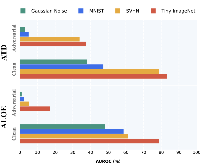
Figure 1: ALOE and ATD are robust outlier detection methods that utilize the Tiny ImageNet dataset as OE. In this experiment, while keeping all other aspects of the original methods constant, we replaced Tiny ImageNet with SVHN, MNIST, and Gaussian noise and repeated the experiments for both ALOE and ATD. This replacement led to a notable decline in detection performance for ALOE and ATD on the CIFAR10 vs. CIFAR100 task, particularly under adversarial attack conditions. We attribute this performance drop to the fact that the SVHN, MNIST, and Gaussian Noise distributions are more distant from CIFAR10 (the inlier distribution in this task) compared to Tiny ImageNet.

Outlier detection has become a crucial component in the design of reliable open-world machine learning models (drummond2006open; bendale2015towards; perera2021one). Robustness against adversarial attacks is another important machine learning safety feature (szegedy2013intriguing; goodfellow2014explaining; akhtar2018threat). Despite the emergence of several promising outlier detection methods in recent years (liznerski2022exposing; cohen2021transformaly; cao2022deep), they often suffer significant performance drops when subjected to adversarial attacks, which aim to convert inliers into outliers and vice versa by adding imperceptible perturbations to the input data. In light of this, recently, several robust outlier detection methods have been proposed (azizmalayeri2022your; lo2022adversarially; chen2020robust; shao2020open; shao2022open; bethune2023robust; goodge2021robustness; chen2021atom; meinke2022provably; franco2023diffusion). However, their results are still unsatisfactory, sometimes performing even worse than random detection, and are often focused on specific cases of outlier detection, such as the open-set recognition or tailored to a specific dataset, rather than being broadly applicable. Motivated by this, we aim to provide a robust and unified solution for outlier detection that can perform well in both clean and adversarial settings.

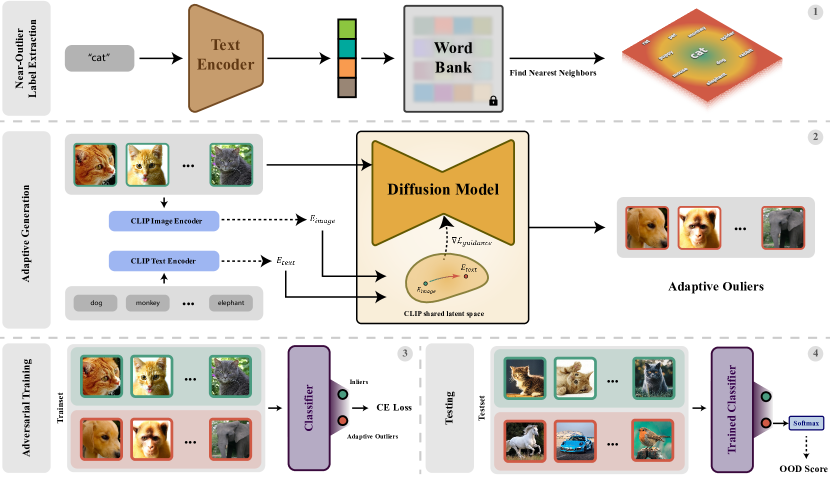
Figure 2: Our proposed adversarially robust outlier detection method is initiated with a Near-Outlier Label Extraction, which finds words analogous to a given input label. These words, combined with inlier training image data, are employed in the Adaptive Generation stage to create Near-Outllier data. This stage is followed by Adversarial Training using both inliers and generated OE data, utilizing the cross-entropy loss function. During Testing, the model processes the input and computes the OOD score as the softmax of the OOD class. (The data filtering steps are not shown in this figure)

Adversarial training, which is the augmentation of training samples with adversarial perturbations, is among the best practices for making models robust (madry2017towards). However, this approach is less effective in outlier detection, as outlier patterns are unavailable during training, thus preventing training of the models with the adversarial perturbations associated with these outliers. For this reason, recent robust outlier detection methods use Outlier Exposure (OE) technique (hendrycks2018deep) in combination with adversarial training to tackle this issue (azizmalayeri2022your; chen2020robust; chen2021atom). In OE, the auxiliary outlier samples are typically obtained from a random and fixed dataset and are leveraged during training. It is clear that these samples should be semantically different from the inlier training set to avoid misleading the detection.

In this study, we experimentally observe (see Fig. 1 and Sec. 3) that the OE technique’s performance is highly sensitive to the distance between the exposed outliers and the inlier training set distribution. Our results suggest that a near-distribution OE set is significantly more beneficial than a distant one. By near-distribution outliers, we refer to image data that possesses semantically and stylistically related characteristics to those of the inlier dataset.

Our observation aligns with (xing2022artificially), which suggests that incorporating data near the decision boundary leads to a more adversarially robust model in the classification task. Simultaneously, numerous studies (schmidt2018adversarially; stutz2019disentangling) have demonstrated that adversarial training demands a greater level of sample complexity relative to the standard setting. Thus, several efforts have been made to enrich the data diversity to enhance the adversarial robustness (hendrycks2019usingx; sehwag2021robust; pang2022robustness).

These observations prompt us to propose the following hypotheses: For adversarial training to be effective in robust outlier detection, the OE samples need to be diverse, near-distribution, and conceptually distinguishable from the inlier samples. We have conducted numerous extensive ablation studies (Sec. LABEL:Ablation_Section), and provided theoretical insights (Sec. 3) to support these claims.

Driven by the mentioned insights, we introduce RODEO (Robust Outlier Detection via Exposing adaptive Out-of-distribution samples), a novel method that enhances the robustness of outlier detection by leveraging an adaptive OE strategy. Our method assumes access to the text label(s) describing the content of the inlier samples, which is a fair assumption according to the prior works (liznerski2022exposing; adaloglou2023adapting). Specifically, the first step involves utilizing a simple text encoder to extract labels that are semantically close to the inlier class label(s), based on their proximity within the CLIP (radford2021learning) textual representation space. To ensure the extracted labels are semantically distinguishable from inlier concepts, we apply a threshold filter, precomputed from a validation set. Then, we initiate the denoising process of a pretrained diffusion image generator (dhariwal2021diffusion) conditioned on the inlier images. The backward process of the diffusion model is guided by the gradient of the distance between the extracted outlier labels’ textual embeddings and the visual embeddings of the generated images. Through this guidance, the diffusion model is enforced to increase the similarity between the generated images and the extracted labels at each step, and transfer inliers to near-distribution outliers during the process. Finally, another predefined threshold, obtained through validation, filters the generated data belonging to the in-distribution based on the CLIP score. We then demonstrate that adversarial training on a classifier that discriminates the inlier and synthesized OE significantly improves robust outlier detection.

We evaluate RODEO in both clean and adversarial settings. In the adversarial setting, numerous strong attacks, including PGD-1000 (madry2017towards), AutoAttack (croce2020reliable), and Adaptive Auto Attack (liu2022practical), are employed for robustness evaluation. Our experiments are conducted across various common outlier detection setups, including Novelty Detection (ND), Open-Set Recognition (OSR), and Out-of-Distribution (OOD) detection. It is noteworthy that previous robust outlier detection methods were primarily limited to specific types of outlier setups. In these experiments, RODEO’s performance is compared against recent and representative outlier detection methods. The compared methods, including EXOE (liznerski2022exposing) and PLP (adaloglou2023adapting), utilized a pretrained CLIP as their detector backbone. The results indicate that RODEO establishes significant performance in adversarial settings, surpassing existing methods by up to 50% in terms of AUROC detection, and achieves competitive results in clean settings. Moreover, through an extensive ablation study, we evaluated our adaptive OE method pipeline in comparison to alternative OE methods (lee2018simple; tao2023non; kirchheim2022outlier; du2022vos; mirzaei2022fake), including both baseline and recent synthetic outlier methods such as Dream-OOD (du2023dream), which utilizes Stable Diffusion (rombach2022high) trained on 5 billion data samples as its generative backbone. In the ablation study, we analyze why RODEO outperforms other alternative OE methods.

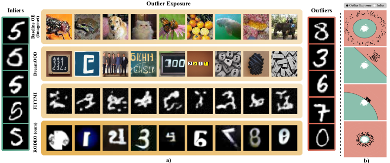
Figure 3: An overview of outlier data from different OE techniques. FITYMI considers image domain information exclusively. Dream-OOD utilizes both text and image domains, but initiating generation from the embedding space makes this method highly biased toward its prior knowledge of the generative backbone, Stable Diffusion. In contrast, RODEO shifts data from inlier to outlier while operating in pixel space. To provide further intuition about the importance of diversity and the distance of the OE from the in-distribution, we compute features for inliers and generated outlier data via a pretrained ViT model (dosovitskiy2020image), and apply t-SNE (van2008visualizing) to visualize the data in 2D. We then find decision boundaries of the data with SVM (cortes1995support) and present them on the right side of each generated OE example. Our OE samples are both near-distribution and diverse.

2 Related Work

Outlier Detection.   Several works have been proposed in outlier detection, with the goal of learning the distribution of inlier samples. Some methods such as CSI (tack2020csi) do this with self-supervised approaches. On the other hand, many methods, such as MSAD (reiss2021mean), Transformaly (cohen2021transformaly), ViT-MSP (NEURIPS2021_3941c435), and Patchcore (roth2021total), aim to leverage knowledge from pre-trained models. EXOE (liznerski2022exposing) and PLP (adaloglou2023adapting) utilized text and image data for the detection task, employing a CLIP model that was pretrained on 400 million data points. Furthermore, some other works have pursued outlier detection in an adversarial setting, including APAE (goodge2021robustness), PrincipaLS (lo2022adversarially), OCSDF (bethune2023robust), and OSAD (shao2022open). ATOM (chen2021atom), ALOE (chen2020robust), and ATD (azizmalayeri2022your) achieved relatively better results compared to others by incorporating OE techniques and adversarial training. However, their performance falls short (as presented in Fig. 1) when the inlier set distribution is far from their fixed OE set. For more details about previous works, see Appendix (Sec. LABEL:detailed_base).

Outlier Exposure Methods. MixUp (zhang2017mixup) adopts a more adaptive OE approach by blending ImageNet samples with inlier samples to create outlier samples closer to the in-distribution. FITYMI (mirzaei2022fake) introduced an OE generation pipeline using a diffusion generator trained on inliers but halted early to create synthetic images that resemble inliers yet display clear differences. The GOE method (kirchheim2022outlier) employs a pretrained GAN to generate synthetic outliers by targeting low-density areas in the inlier distribution. Dream-OOD (du2023dream) uses both image and text domains to learn visual representations of inliers in a latent space and samples new images from its low-likelihood regions. Other OE methods, such as VOS and NPOS (du2022vos; tao2023nonparametric), generate embeddings instead of actual image data.

3 Theoretical Insights

In this section, we provide some insightful examples that highlight the need for near-distribution and diverse OE in outlier detection. Our setup is the following: We assume that the inlier data come from $\mathcal{N}(0,\sigma^{2}I)$ and the test-time outlier is distributed according to $\mathcal{N}(a,\sigma^{2}I)$. Furthermore, let $\mathcal{N}(a^{\prime},\sigma^{2}I)$ be the OE data distribution. We also assume equal class a priori probabilities. We train a classifier using a balanced mixture of inlier and OE samples. However, at test time, the classifier is tested against a balanced mixture of inlier and outlier samples, rather than the OE data.

Near-distribution OE is beneficial

Theorem 3.1.

Let $\sigma=1$, and assume that $\|a^{\prime}\|\geq\|a\|$, reflecting that the OE is far from the distribution. Let $\theta$ be the angle between $a$ and $a^{\prime}$. Under the setup mentioned in Sec. 3, for fixed $\theta$ and $a$, and small $\epsilon$, the optimal Bayes’ adversarial error under $\ell_{2}$ norm bounded attacks with $\epsilon$ norm increases as the OE moves farther from the distribution, i.e., as $\|a^{\prime}\|$ increases. More specifically, the adversarial error is:

$$\begin{split}1-\Phi\left(\frac{\|a^{\prime}\|}{2}-\epsilon\right)+1-\Phi\left(\frac{\|a^{\prime}\|}{2}-c-\epsilon\right),\end{split}$$ (1)

with $c:=\|a^{\prime}\|-\|a\|\cos(\theta)$, and $\Phi(.)$ being the standard normal cumulative distribution function.

Proof.

Under the mentioned setup, the optimal robust classifier is $f^{\star}(x)=\frac{a^{\prime\top}}{\|a^{\prime}\|}(x-\frac{a^{\prime}}{2})=\frac{a^{\prime\top}}{\|a^{\prime}\|}x-\frac{\|a^{\prime}\|}{2}$, for an adversary that has a budget of at most $\epsilon$ perturbation in $\ell_{2}$ norm (schmidt2018adversarially). Now, applying this classifier on the inlier and outlier classes at test time, we get:

$$\frac{a^{\prime\top}x}{\|a^{\prime}\|}\sim\mathcal{N}(0,I),$$ (2)

for an inlier $x$, and also:

$$\frac{a^{\prime\top}x}{\|a^{\prime}\|}\sim\mathcal{N}\left(\frac{a^{\top}a^{\prime}}{\|a^{\prime}\|},I\right),$$ (3)

for an outlier $x$. Therefore, using the classifier $f^{\star}$ to discriminate the inlier and outlier classes, the adversarial error rate would be:

$$1-\Phi\left(\frac{\|a^{\prime}\|}{2}-\epsilon\right)+1-\Phi\left(\frac{a^{\top}a^{\prime}}{\|a^{\prime}\|}-\frac{\|a^{\prime}\|}{2}-\epsilon\right),$$ (4)

where $\Phi(.)$ is the CDF for the inlier distribution $\mathcal{N}(0,1)$.

Let $\delta=a^{\prime}-a$, and note that:

$$\begin{split}\frac{a^{\top}a^{\prime}}{\|a^{\prime}\|}-\frac{\|a^{\prime}\|}{2}=\frac{(a^{\prime}-\delta)^{\top}a^{\prime}}{\|a^{\prime}\|}-\frac{\|a^{\prime}\|}{2}=\frac{\|a^{\prime}\|}{2}-\frac{\delta^{\top}a^{\prime}}{\|a^{\prime}\|}.\end{split}$$ (5)

But note that $\frac{\delta^{\top}a^{\prime}}{\|a^{\prime}\|}=\|a^{\prime}\|-\|a\|\cos(\theta)=:c\geq\|a^{\prime}\|-\|a\|\geq 0$, where $\theta$ is the angle between $a^{\prime}$ and $a$. Hence, by plugging Eq. 5 into Eq. 4, the error rate can be written as:

$$\begin{split}1-\Phi\left(\frac{\|a^{\prime}\|}{2}-\epsilon\right)+1-\Phi\left(\frac{\|a^{\prime}\|}{2}-c-\epsilon\right).\end{split}$$ (6)

But note that the derivative of the above expression with respect to $\|a^{\prime}\|$ is

$$-\frac{1}{2\sqrt{2\pi}}\exp\left(-\frac{1}{2}\left(\frac{\|a^{\prime}\|}{2}-\epsilon\right)^{2}\right)\\ +\frac{1}{2\sqrt{2\pi}}\exp\left(-\frac{1}{2}\left(-\frac{\|a^{\prime}\|}{2}+\|a\|\cos(\theta)-\epsilon\right)^{2}\right),$$

noting that the derivative of $\frac{1}{2}\|a^{\prime}\|-c$ with respect to $\|a^{\prime}\|$ is $-\frac{1}{2}$. We note that for $\epsilon\leq\frac{\|a^{\prime}\|}{2}$, the derivative is positive as long as

$$\frac{\|a^{\prime}\|}{2}-\epsilon\geq\frac{\|a^{\prime}\|}{2}-\|a\|\cos(\theta)+\epsilon,$$ (7)

and

$$\frac{\|a^{\prime}\|}{2}-\epsilon\geq-\frac{\|a^{\prime}\|}{2}+\|a\|\cos(\theta)-\epsilon.$$ (8)

The first condition is satisfied as long as $\epsilon\leq\|a\|\cos(\theta)$, which is always satisfied for small $\epsilon$ if $\theta\neq\pi/2$. The second condition is also satisfied as $\|a^{\prime}\|\geq\|a\|$ by the theorem assumptions. Hence, the derivative is positive and the adversarial error rate is increasing by increasing $\|a^{\prime}\|$. ∎

Diverse OE is beneficial

In the last section, we provided an example of why OE data should be near-distribution to be helpful in a simple setup. Now, we give further insights into why the OE should be diverse. To show this, we introduce the notion of the worst-case outlier detection error.

Definition 3.2.

As the outlier distribution is not known during training, we seek to optimize for its worst-case performance, i.e.:

$$R(f):=\sup_{\|a\|=\alpha}\mathbb{E}_{x\sim p}(\ell(f(x),y)),$$ (9)

where we assume 0/1 loss for simplicity, and $p:=0.5\mathcal{N}(0,\sigma^{2}I)+0.5\mathcal{N}(a,\sigma^{2}I)$.

Theorem 3.3.

Assuming $\sigma\approx 0$, the optimal worst-case outlier detection error under the setup of Sec. 3 is $R(f^{\star})=50\%$. Additionally, if the OE is sampled from a Gaussian mixture, with infinitely many mixture components, whose means are sampled uniformly from the hypersphere $\mathcal{S}^{d-1}(\alpha),$ then $R(f^{\star})=0\%$.

Proof.

First note that $f^{\star}$, which is the optimal classifier, takes a linear form of $f^{\star}(x)=\frac{a^{\prime\top}}{\|a^{\prime}\|}(x-\frac{a^{\prime}}{2})$. Also, note that if the outlier distribution mean value, $a$, is far from that of the OE, $a^{\prime}$, the risk $R(f)$ would grow large and become $50\%$. That is, in finding the supremum, $a$ would be placed far from $a^{\prime}$, resulting in $R(f^{\star})=50\%$; i.e. one plausible solution is $a=-\alpha\frac{a^{\prime}}{\|a^{\prime}\|}$, which leads to erroneous output $f^{\star}(x)<0$, for all outlier samples $x$ concentrated around $a$.

However, we note that for this worst-case scenario, a better OE choice, than a simple Gaussian distribution, would be to first randomly pick a center $a^{\prime}$ uniformly from the sphere centered around zero, with radius $\alpha$, denoted as $\mathcal{S}^{d-1}(\alpha)$, where $d$ is feature space dimensionality. This results in the marginal OE distribution, $p_{OE}$ as follows:

$$p_{OE}(x)\propto\int_{\mathcal{S}^{d-1}(\alpha)}\mathcal{N}(a^{\prime},\sigma^{2}I)da^{\prime},$$ (10)

For this choice of OE, the optimal Bayes’ classifier that discriminates the inliers and OE, would be a hypersphere centered around zero with radius $\frac{\alpha}{2}$. It is evident that for this classifier, the worst-case risk $R$, would be $0$. The intuition behind this is that wherever the $a$ is placed in taking the supremum, the classifier would detect it as an outlier. ∎

This simple example highlights the need for a diverse OE distribution in solving the outlier detection in the worst-case. Inspired by this example, one could approach constructing $p_{OE}$ through conditioning the OE distribution on the inlier samples $x_{0}$, and a target semantic label $y$ that is distinct from $x_{0}$ original semantic class, $y_{0}$; i.e. $\hat{p}(x|x_{0},y)$, and assuming $\hat{p}$ as a generative process that minimally transforms $x_{0}$ into an outlier sample with semantic label $y$. This is similar to OE samples in the previous theorem, where Gaussian kernels with means deviating large enough from the in-distribution (with distance $\alpha$ from the inlier class mean) constitute the OE distribution. To make this analogy happen, the outlier label $y$ has the role of making $x$ sufficiently distant away from the in-distribution. This way, $p_{OE}$ would become:

$$p_{OE}(x)=\sum_{y}\int\hat{p}(x|x_{0},y)p(x_{0})p(y|y_{0})dx_{0},$$ (11)

where $p(x_{0})$ is the inlier class distribution and $p(y|y_{0})$ is the prior distribution over the target classes that are distinct from the inlier semantic class $y_{0}$. This is similar to the form of OE distribution in Eq. 10.

4 Method

Motivation. To develop a robust outlier detection model, the Outlier Exposure (OE) technique appears to be crucial (chen2020robust; chen2021atom; azizmalayeri2022your); otherwise, the model would lack information about the adversarial patterns in the outlier data. However, the Baseline OE technique, which involves leveraging outliers from a presumed dataset, leads to unsatisfactory results in situations where the auxiliary exposed outliers deviate significantly from the in-distribution. Motivated by these factors, we aim to propose an adaptive OE technique that attempts to generate diverse and near-distribution outliers, which can act as a proxy for the real inference-time outliers. The subsequent sections will provide a detailed description of the primary stages of our methodology. Our method is outlined in Fig. 2.

4.1 Generation Step

Near-outlier Label Extraction. Utilizing a text encoder and given the class labels of the inlier samples, we identify words closely related to them. To achieve this, we utilize Word2Vec (mikolov2013efficient), a renowned and simple text encoder, to obtain the embeddings of the inlier labels, denoted as $y_{\text{inlier}}$ (e.g., “screw”), and subsequently retrieve their nearest labels (e.g., “nail”). By comparing these with a pre-computed threshold ($\tau_{\text{text}}$), we refine the extracted labels by excluding those very similar to the inlier labels. This threshold is computed using ImageNet labels as the validation set and the CLIP text encoder embedding to compute word similarities. Utilizing these extracted near labels in subsequent steps leads to the generation of semantically-level outlier samples (those that are semantically different from the inliers). To further enhance the diversity of synthesized outliers, we also consider pixel-level OOD samples (those that differ from the in-distribution at the texture level). For this purpose, we incorporate texts containing negative attributes of the inlier labels (e.g., “broken screw”), and the union of these two sets of labels forms near outliers (n-outliers) labels: $y_{\text{n-outliers}}$, which will guide the image generation process utilizing the CLIP model in the next steps. More details about near-label set extraction and threshold ($\tau_{\text{text}}$) computing are available in the Appendix (Sec. K).

CLIP Guidance. The CLIP model is designed to learn joint representations between the text and image domains, and it comprises a pre-trained text encoder and an image encoder. The CLIP model operates by embedding both images and texts into a shared latent space. This allows the model to assign a CLIP score that evaluates the relevance of a caption to the actual content of an image. In order to effectively extract knowledge from the CLIP in image generation, we propose the $\mathcal{L}_{\text{guidance}}\left(\boldsymbol{x}_{\text{gen}},\boldsymbol{y}_{\text{n-outliers}}\right)$ loss, which aims to minimize the cosine similarity between the CLIP space embeddings of the generated image $\boldsymbol{x}_{\text{gen}}$ and the target text (extracted outlier labels)  $\boldsymbol{y}_{\text{n-outliers}}$, i.e. $\mathcal{D}\left(x,y\right)=\frac{x^{\top}y}{\|x\|\|y\|}$:

Here, $E_{I}$ and $E_{T}$ represent the embeddings extracted by the CLIP image and text encoders, respectively. During the conditional diffusion sampling process, the gradients from the $\mathcal{L}_{\text{guidance}}$ will be used to guide the inlier sample towards the near outliers.

Conditioning on Image. We condition the denoising process on the inlier images instead of initializing it with random Gaussian noise. Specifically, we employ a pre-trained diffusion generator and start the diffusion process from a random time step, initiated with the inliers with noise (instead of beginning with pure Gaussian noise). Based on previous works (meng2021sdedit; kim2022diffusionclip), we set $t_{0}\sim U(0.3T,0.6T)$, where $T$ represents the number of denoising steps in the regular generation setup.

Randomly choosing $t_{0}$ for the denoising process leads to the generation of diverse outliers since, with smaller $t_{0}$, inlier images undergo minor changes, while relatively larger $t_{0}$ values lead to more significant changes, thereby increasing the diversity of generated outlier samples. We then progressively remove the noise with CLIP guidance to obtain a denoised result that is both outlier and close to the in-distribution: $\ \ {x}_{t-1}\sim\mathcal{N}(\mu({x}_{t}|y_{\text{NOOD}})+s\cdot\Sigma({x}_{t}|y_{\text{n-outliers}})\cdot\nabla_{{x}_{t}}(\mathcal{L}_{\text{guidance }}\left({x}_{{t}},y_{\text{n-outliers}}\right)),\ \Sigma({x}_{t}|y_{\text{n-outliers}}))$, where the scale coefficient $s$ controls the level of perturbation applied to the model. Please see Appendix (Sec. LABEL:gen_step_app) for more details about the preliminaries of diffusion models (sohl2015deep; ho2020denoising) and the generation step. Additionally, refer to Fig. 8 for some examples of generated images.

Table 1:

(a) In this table, we assess ND methods on various datasets against PGD-1000, AutoAttack (AA), AdaptiveAutoAttack (A3), and a clean setting, using the AUROC(%) metric. Perturbations: $\epsilon=\frac{8}{255}$ for low-res and $\epsilon=\frac{2}{255}$ for high-res datasets. The best scores are bolded.

Method

Attack

Low-Res Datasets

High-Res Datasets

Mean

CIFAR10

CIFAR100

MNIST

FMNIST

SVHN

MVTecAD

Head-CT

BrainMRI

Tumor Detection

Covid19

Imagenet-30

CSI

Clean / PGD

94.3 / 2.7

89.6 / 2.5

93.8 / 0.0

92.7 / 4.1

96.0 / 1.3

63.6 / 0.0

60.9 / 0.1

93.2 / 0.0

85.3 / 0.0

65.1 / 0.0

91.6 / 0.3

84.2 / 1.0

MSAD

Clean / PGD

97.2 / 0.0

96.4 / 2.6

96.0 / 0.0

94.2 / 0.0

63.1 / 0.5

87.2 / 0.4

59.4 / 0.0

99.9 / 1.5

95.1 / 0.0

89.2 / 4.0

96.9 / 0.0

88.6 / 0.8

Transformaly

Clean / PGD

98.3 / 0.0

97.3 / 4.1

94.8 / 9.9

94.4 / 0.2

55.4 / 0.3

87.9 / 0.0

78.1 / 5.8

98.3 / 4.5

97.4 / 6.4

91.0 / 9.1

97.8 / 0.0

90.1 / 3.7

EXOE

Clean / PGD

99.6 / 0.3

97.8 / 0.0

96.0 / 0.0

94.7 / 1.8

68.2 / 0.0

76.2 / 0.2

82.4 / 0.1

86.2 / 0.1

79.3 / 0.0

72.5 / 0.8

98.1 / 0.0

86.5 / 0.3

PatchCore

Clean / PGD

68.3 / 0.0

66.8 / 0.0

83.2 / 0.0

77.4 / 0.0

52.1 / 3.0

99.6 / 6.5

98.5 / 1.3

91.4 / 0.0

92.8 / 9.2

77.7 / 3.8

74.2 / 0.0

80.2 / 2.3

PrincipaLS

Clean / PGD

57.7 / 23.6

52.0 / 15.3

97.3 / 76.4

91.0 / 60.8

63.0 / 30.3

63.8 / 24.0

68.9 / 26.8

70.2 / 32.9

73.5 / 24.4

54.2 / 15.1

61.4 / 18.7

68.4 / 31.7

OCSDF

Clean / PGD

57.1 / 22.9

48.2 / 14.6

95.5 / 60.8

90.6 / 53.2

58.1 / 23.0

58.7 / 4.8

62.4 / 13.0

63.2 / 18.6

65.2 / 16.3

46.1 / 8.4

62.0 / 24.8

64.3 / 23.7

APAE

Clean / PGD

55.2 / 0.0

51.8 / 0.0

92.5 / 21.3

86.1 / 9.7

52.6 / 16.5

62.1 / 3.9

68.1 / 6.4

55.4 / 9.1

64.6 / 15.0

50.7 / 9.8

54.5 / 12.8

63.0 / 9.5

RODEO (ours)

Clean / PGD

87.4 / 70.2

79.6 / 62.1

99.4 / 94.6

95.6 / 87.2

78.6 / 33.8

61.5 / 14.9

87.3 / 68.6

76.3 / 68.4

89.0 / 67.0

79.6 / 58.3

86.1 / 73.5

83.7 / 63.5

2-14

AA / A3

69.3 / 70.5

61.0 / 61.3

95.2 / 94.0

87.6 / 87.0

33.2 / 31.8

14.2 / 13.4

68.4 / 68.1

70.5 / 67.7

66.9 / 65.6

58.8 / 57.6

76.8 / 72.4

63.8 / 62.6

The definition of the FDC metric introduced in the paper is as below:

$$FDC=\log(1+\frac{Density\times Coverage}{FID}\times 10^{4})$$ (19)

Appendix J The Significance of Conditioning on Both Images and Text from the inlier Distribution

In order to have an accurate outlier detector, it’s important to generate diverse and realistic samples that are close to the distribution of the inlier data. In our study, we tackle this challenge by leveraging the information contained in the inlier data. Specifically, we extract the labels of classes that are close to the inlier set and use them as guidance for generation. Additionally, we initialize the reverse process generation of a diffusion model with inlier images, so the generation of outlier data in our pipeline is conditioned on both the images and the text of the inlier set. This enables us to generate adaptive outlier samples.

In the Ablation Study (sec. LABEL:Ablation_Section), we demonstrate the importance of using both image and text information for generating outlier data. We compare our approach with two other methods that condition on only one type of information and ignore the other. The first technique generates fake images based on the inlier set, while the other generates outlier data using only the extracted text from inlier labels. The results show that both techniques are less effective than our adaptive exposure technique, which conditions the generation process on both text and image. This confirms that using both sources of information is mandatory and highly beneficial.

J.1 Samples Generated Solely Based on Text Conditioning

In this section, we compare inlier images with images generated by our pipline using only text in Fig. 7 (without conditioning on the images). Our results, illustrated by the plotted samples, demonstrate that there is a significant difference in distribution between these generated images and inlier images. This difference is likely the reason for the ineffectiveness of the outlier samples generated with this technique.

Appendix K Label Generation

K.1 Pixel-Level and Semantic-Level outlier Detection

OOD samples can be categorized into two types: pixel-level and semantic-level. In pixel-level outlier detection, ID and outlier samples differ in their local appearance, while remaining semantically identical. For instance, a broken glass could be considered an outlier sample compared to an intact glass due to its different local appearance. In contrast, semantic-level outlier samples differ at the semantic level, meaning that they have different meanings or concepts than the ID samples. For example, a cat is an outlier sample when we consider dog semantics as ID because they represent different concepts.

K.2 Our Method of Generating labels

A reliable and generalized approach for outlier detection must have the capability to detect both semantic-level and pixel-wise outliers, as discussed in the previous section. To this end, our proposed method constructs n-outlier labels by combining two sets of words: near-distribution labels and negative adjectives derived from a inlier label name. We hypothesize that the former set can detect semantic-level outliers, while the latter set is effective in detecting pixel-wise outliers. Additionally, we include an extra label, marked as ’others’, in the labels list to increase the diversity of exposures.

To generate negative adjectives, we employ a set of constant texts that are listed below and used across all experimental settings (X is the inlier label name):

• A photo of X with a crack

• A photo of a broken X

• A photo of X with a defect

• A photo of X with damage

• A photo of X with a scratch

• A photo of X with a hole

• A photo of X torn

• A photo of X cut

• A photo of X with contamination

• A photo of X with a fracture

• A photo of a damaged X

• A photo of a fractured X

• A photo of X with destruction

• A photo of X with a mark

For n-outlier labels, we utilize Word2Vec to search for semantically meaningful word embeddings after inlierizing the words through a process of lemmatization. First, we obtain the embedding of the inlier class label and then search among the corpus to identify the 1000 nearest neighbors of the inlier class label. In the subsequent phase, we employ the combination of Imagenet labels and CLIP to effectively identify and eliminate labels that demonstrate semantic equivalence to the inlier label. Initially, we leverage CLIP to derive meaningful representations of the Imagenet labels. Then, we calculate the norm of the pairwise differences among these obtained representations. By computing the average of these values, a threshold is established, serving as a determinant of the degree of semantic similarity between candidate labels and the inlier label. The threshold is defined as:

$$\tau_{text}=\frac{\sum_{i=1,i\neq j}^{M}\sum_{j=1}^{M}|E_{T}(y_{i})-E_{T}(y_{j})|}{M(M-1)}$$ (20)

In which, $M$ is the number of Imagenet labels, and $y_{i}$s are the Imagenet labels. Consequently, we filter out labels whose CLIP output exhibits a discrepancy from the inlier class(es) that falls below the threshold.

We then sample n-outlier labels from the obtained words based on the similarity factor of the neighbors to the inlier class label. The selection probability of the n-outlier labels is proportional to their similarity to the inlier class label. Finally, we compile a list of n-outlier labels to serve as near outlier labels.

Table 3: The detailed AUROC scores of the class-specific experiments for (One-Class) Novelty Detection setting in CIFAR10, CIFAR100, MNIST, Fashion-MNIST datasets.

(a) CIFAR10

Method	Attack		Class									Average
		0	1	2	3	4	5	6	7	8	9
Ours	Clean	91.7	97.3	77.4	74.0	82.6	81.2	91.5	92.8	94.0	91.7	87.4
	BlackBox	89.9	95.8	75.5	72.1	81.6	79.1	89.1	91.2	92.4	89.6	85.6
	PGD-1000	76.6	81.4	59.1	55.2	65.0	65.9	73.6	69.6	78.9	77.3	70.2
	AutoAttack	75.7	80.0	58.7	53.6	64.2	65.1	72.1	68.8	78.9	76.0	69.3

(b) CIFAR100

Method	Attack		Class																			Average
		0	1	2	3	4	5	6	7	8	9	10	11	12	13	14	15	16	17	18	19
Ours	Clean	79.0	78.6	95.5	78.1	89.2	69.4	76.2	82.6	77.9	87.4	92.7	73.1	77.6	65.0	83.9	65.5	72.1	93.6	83.5	72.0	79.6
	BlackBox	76.9	77.0	93.2	75.4	87.6	67.3	74.0	79.6	75.7	85.1	89.9	71.3	74.7	62.9	81.0	63.4	69.7	91.8	81.8	70.1	77.4
	PGD-1000	59.7	60.2	83.0	61.3	72.9	53.0	60.4	62.6	59.0	76.5	78.1	51.2	61.0	47.4	60.3	44.5	51.9	78.7	61.2	58.1	62.1
	AutoAttack	56.8	59.4	80.4	60.9	73.9	51.2	61.3	61.7	58.3	75.9	75.7	51.7	59.9	45.7	59.2	44.4	50.6	76.1	60.5	57.1	61.0

(c) MNIST

Method	Attack		Class									Average
		0	1	2	3	4	5	6	7	8	9
Ours	Clean	99.8	99.4	99.3	99.2	99.6	99.4	99.8	98.9	99.4	98.8	99.4
	BlackBox	98.7	99.0	98.2	98.8	98.3	98.9	99.4	97.8	98.5	98.2	98.6
	PGD-1000	96.3	96.1	95.5	92.0	97.4	95.1	96.4	92.5	94.0	91.2	94.6
	AutoAttack	96.9	96.1	96.3	92.0	96.7	96.3	98.1	92.5	95.2	92.0	95.2

(d) Fashion-MNIST

Method	Attack		Class									Average
		0	1	2	3	4	5	6	7	8	9
Ours	Clean	95.8	99.7	93.9	93.4	92.9	98.3	86.5	98.6	98.5	98.8	95.6
	BlackBox	94.4	98.6	92.7	92.6	91.2	96.9	85.1	97.1	97.5	97.1	94.3
	PGD-1000	89.7	98.4	82.9	79.9	76.1	94.8	71.4	94.0	90.7	93.9	87.2
	AutoAttack	89.7	98.1	83.0	80.9	76.5	95.1	72.6	94.2	92.4	94.1	87.6

Appendix L Outlier Detection Performance Under Various Strong Attacks

Tables 3, 4, and 5 demonstrate the robust detection performance of RODEO when subjected to various strong attacks.

Table 4: OOD detailed results

(a) CIFAR10

Out-Dataset	Attack	Method
		OpenGAN	ViT (RMD)	ATOM	AT (OpenMax)	OSAD (OpenMax)	ALOE (MSP)	ATD	RODEO
MNIST	Clean	99.4	98.7	98.4	80.4	86.2	74.6	98.8	96.9
	PGD-1000	29.4	2.6	0.0	38.7	54.4	21.8	89.3	83.1
TiImgNet	Clean	95.3	95.2	97.2	81.0	81.9	82.1	88.0	85.1
	PGD-1000	14.3	1.4	3.4	15.6	18.4	20.7	46.1	46.3
Places	Clean	95.0	98.3	98.7	82.5	83.3	85.1	92.5	96.2
	PGD-1000	16.4	2.2	5.6	18.0	20.3	21.9	59.8	70.2
LSUN	Clean	96.5	98.4	99.1	85.0	86.4	98.7	96.0	99.0
	PGD-1000	23.1	1.1	1.0	18.7	19.8	50.7	68.1	85.1
iSUN	Clean	96.3	98.6	99.5	83.9	84.0	98.3	94.8	97.7
	PGD-1000	22.1	1.2	2.5	18.6	19.4	49.5	65.9	78.7
Birds	Clean	98.3	76.0	95.8	75.1	76.5	79.9	93.6	97.8
	PGD-1000	33.6	0.0	5.2	13.8	18.2	20.9	68.1	76.0
Flower	Clean	98.3	99.6	99.8	85.5	88.6	79.0	99.7	99.5
	PGD-1000	29.2	1.7	19.0	20.0	25.7	18.7	92.8	88.7
COIL	Clean	98.1	95.9	97.3	70.3	75.0	76.8	90.8	91.1
	PGD-1000	37.6	3.0	8.6	15.7	17.8	18.4	57.2	59.5
CIFAR100	Clean	95.0	97.3	94.2	79.6	79.9	78.8	82.0	75.6
	PGD-1000	9.2	0.8	1.6	15.1	17.2	16.1	37.1	37.8
Avg.	Clean	97.1	95.1	97.8	80.5	82.7	84.3	94.3	93.2
	PGD-1000	25.7	1.6	5.1	19.9	24.2	27.8	68.4	69.5

(b) CIFAR100

Out-Dataset	Attack	Method
		OpenGAN	ViT (RMD)	ATOM	AT (RMD)	OSAD (MD)	ALOE(MD)	ATD	RODEO
MNIST	Clean	99.0	83.8	90.4	41.1	95.9	96.6	97.3	99.7
	PGD-1000	12.9	0.0	0.0	12.5	80.3	71.4	84.6	96.0
TiImgNet	Clean	88.3	90.1	85.1	72.3	48.3	58.1	73.7	72.9
	PGD-1000	2.2	1.4	0.1	10.3	8.2	4.6	24.3	37.3
Places	Clean	94.5	92.3	94.8	73.1	55.7	75.0	83.3	93.0
	PGD-1000	3.2	2.0	3.0	11.0	10.4	12.4	40.0	66.6
LSUN	Clean	97.1	91.6	96.6	76.0	55.6	83.1	89.2	98.1
	PGD-1000	5.6	0.0	1.5	11.2	8.7	19.0	47.7	83.1
iSUN	Clean	96.4	91.4	96.4	72.5	54.8	80.1	86.5	95.1
	PGD-1000	5.8	0.0	1.4	10.2	8.9	20.4	45.6	75.6
Birds	Clean	96.6	97.8	95.1	73.1	54.5	78.4	93.4	96.8
	PGD-1000	5.7	8.8	12.5	11.7	9.3	22.0	64.5	74.2
Flower	Clean	96.8	96.6	98.9	77.6	69.6	85.1	97.2	97.2
	PGD-1000	7.6	3.8	15.5	14.0	21.2	30.1	78.4	77.2
COIL	Clean	97.7	88.1	79.5	74.4	57.5	77.9	80.6	78.6
	PGD-1000	14.0	1.8	0.0	14.6	12.3	17.5	43.6	43.1
CIFAR10	Clean	92.9	94.8	87.5	67.5	50.3	43.6	57.5	61.5
	PGD-1000	7.4	4.1	2.0	9.0	8.6	1.3	12.1	29.0
Avg.	Clean	95.8	91.5	91.6	70.0	61.5	79.3	87.7	88.1
	PGD-1000	7.1	2.0	3.7	11.9	19.9	24.7	53.6	64.7

Table 5: AUROC scores for (One-Class) Novelty Detection under three different adversarial attacks with $\epsilon=\frac{8}{255}$

Method	Attack	Low-Res Datasets					High-Res Datasets
		CIFAR10	CIFAR100	MNIST	FMNIST	SVHN	MVTecAD	Head-CT	BrainMRI	Tumor Detection	Covid19	Imagenet-30
DeepSVDD	Clean	64.8	67.0	94.8	94.5	60.3	67.0	62.5	74.5	70.8	61.9	62.8
	BlackBox	54.6	55.3	65.7	66.8	42.7	36.0	44.1	52.7	42.0	32.4	50.1
	PGD-1000	22.4	14.1	10.8	48.7	7.2	6.3	0.0	3.9	1.6	0.0	22.0
	AutoAttack	9.7	5.8	9.6	38.2	2.4	0.0	0.0	2.1	0.0	0.0	7.3
CSI	Clean	94.3	89.6	93.8	92.7	96.0	63.6	60.9	93.2	85.3	65.1	91.6
	BlackBox	43.1	34.7	72.3	64.2	32.0	37.7	50.3	61.0	60.9	25.7	36.8
	PGD-1000	2.7	2.5	0.0	4.1	1.3	0.0	0.1	0.0	0.0	0.0	0.3
	AutoAttack	0.0	0.0	0.0	3.1	0.7	0.0	0.0	0.0	0.0	0.0	0.0
MSAD	Clean	97.2	96.4	96.0	94.2	63.1	87.2	59.4	99.9	95.1	89.2	96.9
	BlackBox	38.4	51.8	58.1	73.8	40.9	41.3	42.6	64.2	67.7	53.6	34.9
	PGD-1000	0.0	2.6	0.0	0.0	0.5	0.4	0.0	1.5	0.0	4.0	0.0
	AutoAttack	0.0	1.7	0.0	0.0	0.0	0.0	0.0	0.0	0.0	1.9	0.0
Transformaly	Clean	98.3	97.3	94.8	94.4	55.4	87.9	78.1	98.3	97.4	91.0	97.8
	BlackBox	62.9	64.0	73.5	79.6	26.4	56.0	65.0	71.6	78.6	70.7	63.5
	PGD-1000	0.0	4.1	9.9	0.2	7.3	0.0	5.8	4.5	6.4	9.1	0.0
	AutoAttack	0.0	2.6	6.7	0.0	1.9	0.0	3.2	1.6	5.1	4.4	0.0
PatchCore	Clean	68.3	66.8	83.2	77.4	52.1	99.6	98.5	91.4	92.8	77.7	98.1
	BlackBox	18.1	23.6	46.9	58.2	12.5	58.3	80.7	72.5	67.2	56.3	24.4
	PGD-1000	0.0	0.0	0.0	0.0	3.0	6.5	1.3	0.0	9.2	3.8	0.0
	AutoAttack	0.0	0.0	0.0	0.0	1.1	4.8	0.0	0.0	6.1	0.5	0.0
PrincipaLS	Clean	57.7	52.0	97.3	91.0	63.0	63.8	68.9	70.2	73.5	54.2	74.2
	BlackBox	33.3	39.4	91.6	71.1	47.7	45.2	54.3	56.9	56.4	43.8	31.9
	PGD-1000	23.6	15.3	76.4	60.8	30.3	24.0	26.8	32.9	24.4	15.1	18.7
	AutoAttack	20.2	14.7	72.5	58.2	29.5	12.6	16.2	17.8	14.7	9.1	18.0
OCSDF	Clean	57.1	48.2	95.5	90.6	58.1	58.7	62.4	63.2	65.2	46.1	61.4
	BlackBox	48.4	36.9	85.7	77.0	46.8	33.4	40.2	48.0	35.0	28.5	52.7
	PGD-1000	22.9	14.6	60.8	53.2	23.0	4.8	13.0	18.6	16.3	8.4	18.7
	AutoAttack	15.3	12.0	58.3	49.2	19.8	0.3	8.5	12.5	10.1	6.5	14.1
APAE	Clean	55.2	51.8	92.5	86.1	52.6	62.1	68.1	55.4	64.6	50.7	62.0
	BlackBox	37.6	16.3	73.0	24.3	41.6	35.9	45.2	27.1	43.1	26.1	33.9
	PGD-1000	0.0	0.0	21.3	9.7	16.5	3.9	6.4	9.1	15.0	9.8	24.8
	AutoAttack	0.0	0.0	19.8	7.0	16.2	1.8	3.8	8.3	8.3	8.7	0.0
EXOE	Clean	99.6	97.8	96.0	94.7	68.2	76.2	82.4	86.2	79.3	72.5	98.1
	BlackBox	68.3	71.5	79.4	70.4	31.1	52.7	44.6	59.0	51.4	45.5	37.2
	PGD-1000	0.3	0.0	0.0	1.8	0.0	0.2	0.1	0.1	0.0	0.8	0.0
	AutoAttack	0.0	0.0	0.0	1.1	0.0	0.1	0.1	0.0	0.0	0.2	0.0
RODEO (ours)	Clean	87.4	79.6	99.4	95.6	78.6	61.5	87.3	76.3	89.0	79.6	86.1
	BlackBox	85.6	77.4	98.6	94.3	77.2	60.0	85.6	75.8	87.2	75.0	83.9
	PGD-1000	70.2	62.1	94.6	87.2	33.8	14.9	68.6	68.4	67.0	58.3	73.5
	AutoAttack	69.3	61.0	95.2	87.6	33.2	14.2	68.4	70.5	66.9	58.8	76.8
	A3	70.5	61.3	94.0	87.0	31.8	13.4	68.1	67.7	65.6	57.6	72.4

Table 6: Detailed AUROC(%) comparison of different exposure techniques and our introduced method of Adaptive Exposure over different datasets.

	Attack	CIFAR10	CIFAR100	MNIST	Fashion-MNIST	MVTec-ad	Head-CT	Brain-MRI	Tumor Detection	Covid19
Gaussian Noise	Clean	64.4	54.6	60.1	62.7	41.9	59.0	45.3	51.7	40.7
	PGD	15.2	11.9	11.6	15.0	0.0	0.5	0.0	0.9	0.0
ImageNet (Fixed OE Dataset)	Clean	87.3	79.6	90.0	93.0	64.6	61.8	69.3	71.8	62.7
	PGD	69.3	64.5	42.8	82.0	0.0	1.3	0.0	22.1	23.4
Mixup with ImageNet	Clean	59.4	56.1	59.6	74.2	58.5	54.4	57.3	76.4	69.2
	PGD	30.8	27.1	1.7	47.8	0.5	20.6	10.8	53.1	50.2
Fake Image Generation	Clean	29.5	23.0	76.0	52.2	43.5	63.7	65.2	65.2	42.7
	PGD	15.5	14.3	51.1	30.6	7.2	6.9	28.2	32.1	12.4
Stable Diffusion Prompt	Clean	62.4	54.8	84.3	63.7	54.9	71.5	66.7	45.8	37.1
	PGD	35.0	34.4	62.1	47.1	12.2	2.2	7.0	5.3	0.0
Dream outlier Prompt	Clean	58.2	50.3	80.5	66.8	55.0	69.9	68.6	42.7	44.1
	PGD	24.7	20.7	51.4	45.9	12.7	1.2	5.0	10.9	0.1
Adaptive Exposure	Clean	87.4	79.6	99.4	95.6	61.5	87.3	76.3	89.0	79.6
	PGD	70.2	61.3	94.6	87.2	14.9	68.6	68.4	67.0	58.3

Table 7: FID, Density, and Coverage Metrics for Adaptive Exposure technique

	Metric	CIFAR10	CIFAR100	MNIST	Fashion-MNIST	MVTec-ad	Head-CT	Brain-MRI	Tumor Detection	Covid19
Adaptive Exposure	FID	145	156	133	134	263	204	165	186	201
	D / C	0.87 / 0.64	0.63 / 0.62	0.75 / 0.86	0.61 / 0.44	0.64 / 0.09	0.77 / 0.83	0.69 / 0.61	0.57 / 0.37	0.51 / 0.80

Table 8: The detailed AUROC of the experiments for ND, OSR, and OOD settings under different training modes.

(a) ND

Method	Training Mode	Attack	Dataset
			CIFAR10	CIFAR100	MNIST	FashionMNIST	Head-CT	Covid19
Ours	Non-Adversarial	Clean / PGD-1000	93.1 / 0.0	86.6 / 0.0	98.4 / 0.0	94.8 / 0.0	96.1 / 0.0	89.2 / 0.0
	Adversarial	Clean / PGD-1000	87.4 / 70.2	79.6 / 61.3	99.4 / 94.6	95.6 / 87.2	87.3 / 68.6	79.6 / 58.3

(b) OSR

Method	Training Mode	Attack	Dataset
			CIFAR10	CIFAR100	MNIST	FashionMNIST
Ours	Non-Adversarial	Clean / PGD-1000	84.3 / 0.0	69.0 / 0.0	99.1 / 0.0	91.9 / 0.0
	Adversarial	Clean / PGD-1000	79.6 / 62.7	64.1 / 35.3	97.2 / 85.0	87.7 / 65.3

(c) OOD

Method	Training Mode	Attack	Dataset
			CIFAR10 vs CIFAR100	CIFAR100 vs CIFAR10
Ours	Non-Adversarial	Clean / PGD-1000	83.0 / 0.0	71.2 / 0.0
	Adversarial	Clean / PGD-1000	75.6 / 37.8	61.5 / 29.0

Table 9: Adversarial training step hyper-parameters

Adv. Tr.	N	High Res. $\epsilon$	Low Res. $\epsilon$	$\alpha$	Classifier	Optimizer	LR
PGD	10	$\frac{2}{255}$	$\frac{8}{255}$	$2.5\times\frac{\epsilon}{N}$	ResNet	Adam	0.001

Table 10: Generation step hyper-parameters

Gen. Backbone	Pre. Dataset	T	$t_{0}$	$\tau_{\text{image}}$	$\tau_{\text{text}}$
GLIDE(nichol2021glide)	67 Million created dataset	1000	(0, 600)	Eq.11	Eq.17

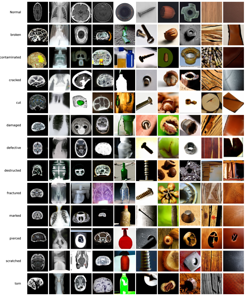
Figure 7: In this experiment, we skipped image conditioning and started the denoising process from pure Gaussian noise, directed by the extracted outlier labels. The resulting generated outlier samples are conditioned solely on text (excluding image conditioning), produced using our pipeline. Comparing the visuals of the generated data in this case with those where the image has also been conditioned showcases the importance of simultaneous image and text conditioning in generating near outlier data.

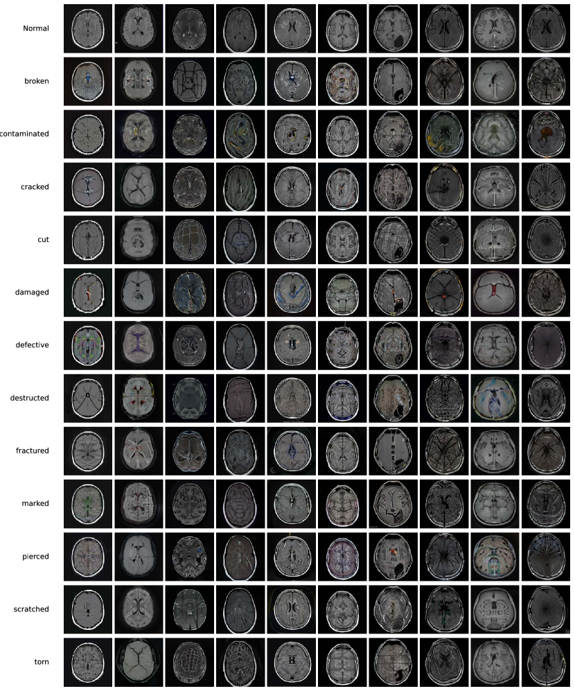
Figure 8: BrainMRI: Examples of generated auxiliary outliers from the BrainMRI dataset, conditioned on negative adjectives and inlier images. The first row depicts inlier images, while the subsequent rows demonstrate generated auxiliary outliers corresponding to the negative adjectives written to the left of each row.

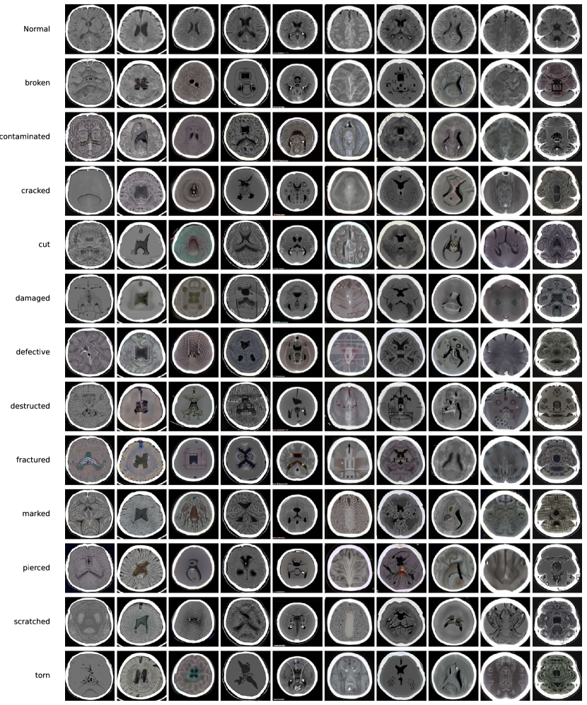
Figure 9: Head-CT: Examples of generated auxiliary outliers from the Head-CT dataset, conditioned on negative adjectives and inlier images. The first row depicts inlier images, while the subsequent rows demonstrate generated auxiliary outliers corresponding to the negative adjectives written to the left of each row.

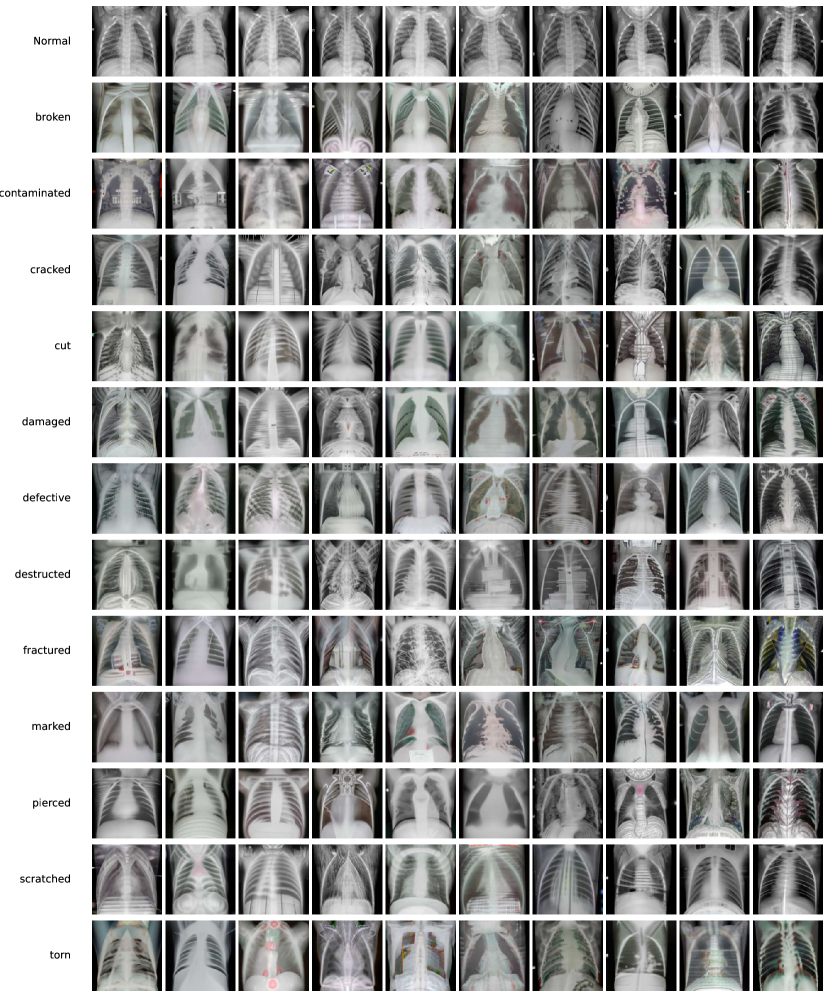
Figure 10: Covid19: Examples of generated auxiliary outliers from the Covid19 dataset, conditioned on negative adjectives and inlier images. The first row depicts inlier images, while the subsequent rows demonstrate generated auxiliary outliers corresponding to the negative adjectives written to the left of each row.

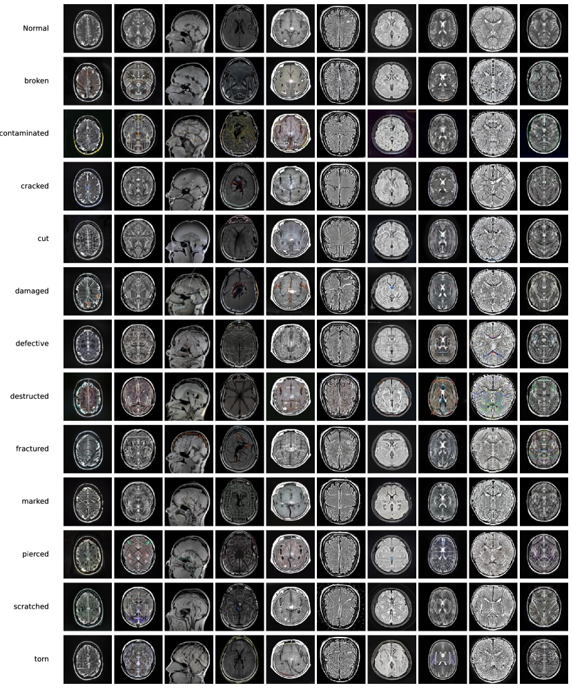
Figure 11: Tumor Detection: Examples of generated auxiliary outliers from the Tumor Detection dataset, conditioned on negative adjectives and inlier images. The first row depicts inlier images, while the subsequent rows demonstrate generated auxiliary outliers corresponding to the negative adjectives written to the left of each row.

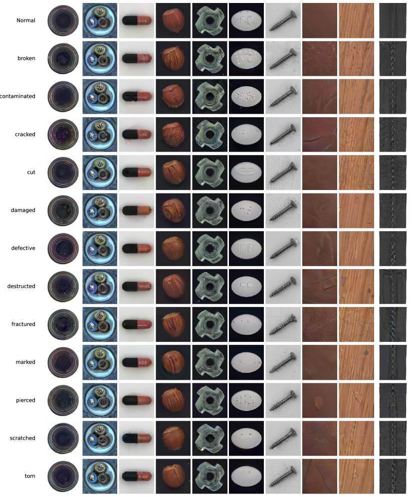
Figure 12: MVTec-AD: Examples of generated auxiliary outliers from the MVTec-AD dataset, conditioned on negative adjectives and inlier images. The first row depicts inlier images, while the subsequent rows demonstrate generated auxiliary outliers corresponding to the negative adjectives written to the left of each row.

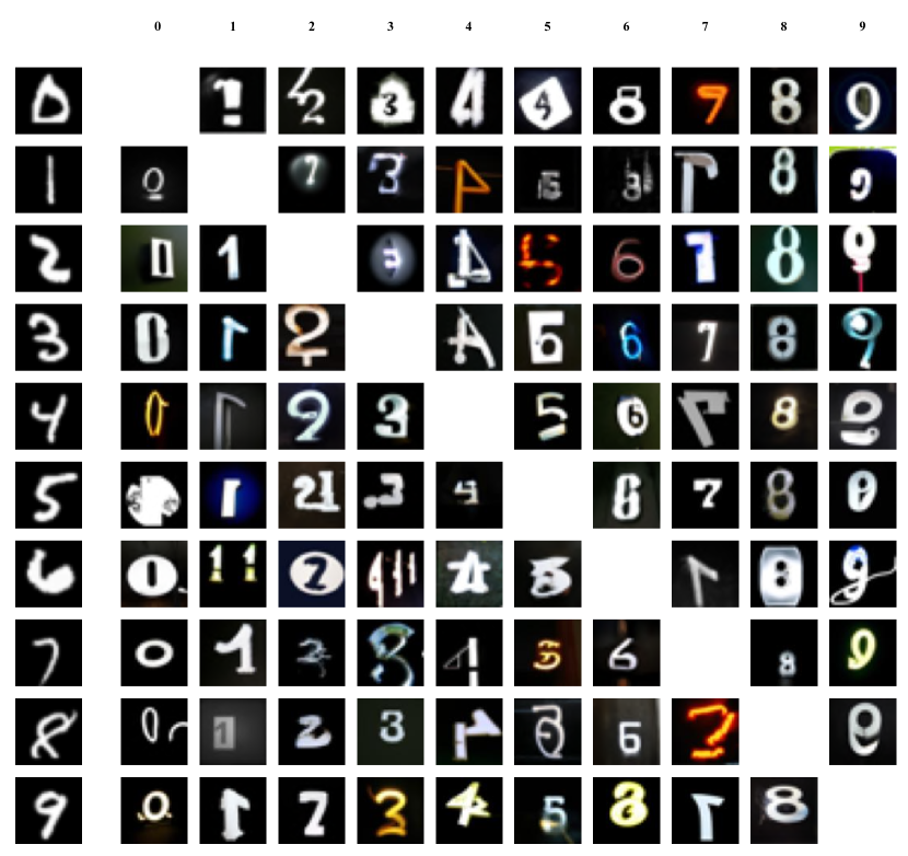
Figure 13: MNIST Adaptive Exposures Grid: This figure illustrates a grid of adaptive exposures of handwritten digits, created using our pipeline with the MNIST dataset, accompanied by their corresponding labels. By utilizing the original data and text prompts, our pipeline generates a variety of exposures that adaptively capture the dataset’s distribution while incorporating outlier elements.

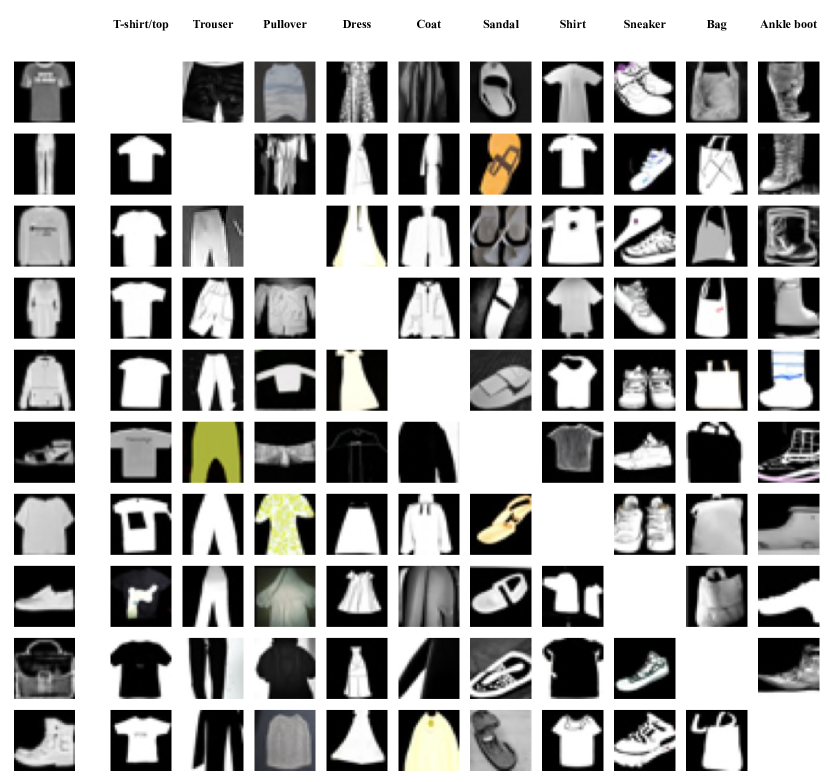
Figure 14: FashionMNIST Adaptive Exposures Grid: This figure illustrates a grid of adaptive exposures of handwritten digits, created using our pipeline with the FashionMNIST dataset, accompanied by their corresponding labels. By utilizing the original data and text prompts, our pipeline generates a variety of exposures that adaptively capture the dataset’s distribution while incorporating outlier elements.