Abstract

This study assesses the long-term effects of redlining policies (1935-1974) on present-day fine particulate matter (PM_2.5) and nitrogen dioxide (NO₂) air pollution levels. Redlining policies enacted in the 1930s, so there is very limited documentation of pre-treatment covariates. Consequently, traditional methods fails to sufficiently account for unmeasured confounders, potentially biasing causal interpretations. By integrating historical redlining data with 2010 PM_2.5 and NO₂ levels, our study aims to discern whether a causal link exists. Our study addresses challenges with a novel spatial and non-spatial latent factor framework, using the unemployment rate, house rent and percentage of Black population in 1940 U.S. Census as proxies to reconstruct pre-treatment latent socio-economic status. We establish identification of a causal effect under broad assumptions, and use Bayesian Markov Chain Monte Carlo to quantify uncertainty. We found strong evidence that historically redlined regions are exposed to higher NO₂ levels, with estimated effect of 0.38 ppb (95% CI, 0.28 to 0.48). We did not observe a strong effect for PM_2.5, though we cannot dismiss the possibility that redlining once influenced PM_2.5 concentrations. Los Angeles, CA and Atlanta, GA show significant and the strongest evidence of harmful effects for both NO₂ and PM_2.5 among the cities studied.

Key words: Air pollution exposure; Latent factor model; Proxy variable; Redlining policy; Spatial causal model.

1 Introduction

1.1 Redlining policy

The redlining policy, initiated in 1935 by the Federal Home Loan Bank Board, mandated the Home Owners' Loan Corporation (HOLC) to create `residential security maps’. These maps classified residential regions with grades reflecting investment security: `A' for Desirable, `B' for Still Desirable, `C' for Declining, and `D' for Redlined. This grading system, operational until the 1974, directly influenced lending decisions. Regions graded `A' were considered minimal risk by banks and mortgage lenders for loans and safe investments, while those labeled `D' were deemed hazardous.

Some studies have investigated the financial inequalities stemming from the redlining policy, with a emphasis on causal analysis and addressing potential confounders. Aaronson et al. (2021) employed a boundary-design approach to mitigate these confounders. Their analysis concentrated on areas adjacent to redlining boundaries (D), comparing `treated' and `controlled' boundaries using propensity score weighting. They discovered that regions assigned to be redlined experienced deteriorating housing market outcomes in the following decades. Similarly, Fishback et al. (2020) conducted a detailed boundary analysis, examining socio-economic characteristics near C-D grade borders. They observed a decline in home values and an increase in black population shares on the D-side compared to the C-side.

The growing interest in environmental inequality has led to association-based studies concerning the redlining policy. Lane et al. (2022) revealed a consistent and nearly monotonic relationship between air pollutants and redlining grades, noting particularly an increase (over 50%) in NO₂ levels from A-graded to D-graded regions. The study also found that within each grade, disparities in air pollution exposure based on race and ethnicity continue to exist. This underscores the racially discriminatory impact of redlining on communities. Additionally, Jung et al. (2022) discovered that between 1998 and 2012, in New York City, schools in historically redlined regions saw smaller reductions in combustion-related air pollutants compared to others. However, the direct causal link between redlining policies and air pollution exposure remains uncertain, despite the apparent association.

Our research aims to bridge the gap in understanding the causal effect of the redlining policy on contemporary air pollution exposure. Our objective is to link this historical redlining data with current air pollution levels, and assesses the potential long-term environmental effects of redlining policies (1935-1974) on present-day PM_2.5 air pollution levels.

This analysis faces two key challenges. First, both redlining grades and air pollution levels exhibit spatial patterns, which must be carefully considered. Second, there is a risk of unmeasured confounding factors, particularly socio-economic status, that could influence both the historical redlining grades and current air pollution levels. In the following section, we outline our approach to addressing these challenges.

1.2 Spatial Causal Inference and Unmeasured Confounding

Addressing unmeasured confounding has become a major topic in causal inference. A unmeasured confounder could introduce bias into the estimated effect and lead to incorrect conclusions about the true causal relationship. There are a wide range of methods to adjust for unmeasured confounding, such as instrumental variables (Bound et al., 1995), negative controls (Lipsitch et al., 2010), latent and proxy variables (Kuroki and Pearl, 2014). These methods are not specifically designed for spatial data, but have been adopted to account for spatial unmeasured confounding in application studies, such as Davis et al. (2021), Shao et al. (2022), Giffin et al. (2021), Haschka et al. (2020), Tustin et al. (2017), and Jerzak et al. (2023).

Moreover, causal methods applied to complex spatial data have been drawing attention. A spatial confounder is a unmeasured confounder that contains spatial structure. The `blessing' of spatial confounder, compared with unstructured confounder, is that the spatial information may be used to capture some of the variability in the confounder, thus mitigating the bias (Gilbert et al., 2021). Dupont et al. (2022) developed method named `spatial+', for cases when the treatment is spatially dependent but not fully determined by spatial location. A partial linear regression was used to adjust for spatial confounding. Guan et al. (2023) assumed a global-scale confounding (global relative to the treatment variable) and adjusted for confounding in the spatial domain by adding a spatially smoothed version of the treatment to the mean of the response variable. In spatial+ and the spectral adjustment, the treatment was assumed continuous. Other methods include region adjustment via spatial smoothing (Schnell and Papadogeorgou, 2020), distance adjusted propensity score matching (Papadogeorgou et al., 2019), spatial propensity-score (Davis et al., 2019), which have been reviewed in Reich et al. (2021).

There are challenges in the redlining data that cannot be addressed by existing methods. Social-economic status is arguably the most important confounding variable. Though some relevant data can be found in the U.S. Census, it is dangerous to assume that we can use them to fully account for social-economic status, thus potentially biasing causal interpretations. Moreover, the time lapse of 75 years between the policy action and the pollution measurement further obscures causal links. In addition, the existence of spatial correlation in all of treatment, outcome, proxies, and potentially the latent confounder, complicates the problem.

In response to these challenges, we expect a method that accommodates for latent confounding factors using proxy variables, and accommodates for unmeasured spatial confounders. We want such a method to sufficiently account for unmeasured confounders and draw consistent estimates. However, none of existing method would allow use the leverage the spatial structure and observed variable while taking use of the proxy variable for unobserved spatial confounding, while the use of proxy for non-spatial causal analysis has been prevalent such as Kong et al. (2019), Yang et al. (2020), and Miao et al. (2018). This paper aims to fill in the gap.

1.3 Contributions and structure of the paper

Our study develops a novel latent framework for causal inference that accounts for both spatial and non-spatial confounding. We establish the identification of causal effects under broad assumptions, and use Bayesian MCMC to quantify uncertainty. Our method promises to enhance the validity of causal claims by rigorously adjusting for confounders. In the case study, we assesses the potential long-term environmental effects of redlining policies on present-day air pollution levels.

The remainder of the paper proceeds as follows. Section 2 describes the motivating data. Sections 3 and 4 detail the statistical methods and their theoretical properties. Section 5 discusses computational aspects. The method is assessed through a simulation study in Section 6, and its application to the motivating data is presented in Section 7. The paper concludes with Section 8.

2 Data description

The data for our study is drawn from multiple sources. We obtain the treatment variable, that is the redlining grades, from the Mapping Inequality Project (Nelson et al., 2023). We label the grades C and D as the `redlined', and grades A and B as the `non-redlined'. The details about this decision can be found in Appendix A.1.

For the outcome variables, we use levels of fine particulate matter (PM_2.5) and nitrogen dioxide (NO₂) in 2010. This year is selected because comprehensive air pollution monitoring for PM_2.5 and NO₂ began in the late 1990s, with sufficient data becoming available from 2010 onward (US EPA, 2024). The pollution data is derived from empirical models provided by the Center for Air, Climate, and Energy Solutions (CACES) (Kim et al., 2020). To address potential confounding, we incorporate variables from the 1940 U.S. Census: unemployment rate, mean house rent, and percentage of Black population.

The geographical boundaries of the HOLC maps, the 1940 Census tracts, and the 2010 air pollution monitoring data differ. We merge these datasets by spatially overlapping them within the HOLC regions. Detailed methodologies for this spatial integration are available in Appendix A.1. After data cleaning, our final dataset includes 4,079 regions across 69 cities and 27 states in the U.S., covering about 20% of the 1940 U.S. population.

Table 1 presents key summary statistics from the 1940 Census and 2010 air pollution data comparing redlined and non-redlined groups across all cities. Example maps for Atlanta, GA are shown in Figure 1. There is clearly spatial dependence in the pollution, redlining and census variables. We observe higher mean values of NO₂, PM_2.5, unemployment rate, and percentage of Black population in redlined areas compared to non-redlined areas. The percentage of Black population is zero-inflated, with approximately 5% of the observed values being zero. Conversely, mean house rent follows an opposite trend, with higher rents observed in non-redlined areas.

Non-redlined Redlined Count 1469 2610 2010 NO₂ (ppb) 12.32 (4.32) 14.80 (5.00) 2010 PM_2.5 ($\mu g/m^{3}$) 10.76 (2.08) 11.02 (1.93) 1940 Unemployment (%) 8.4 (4.30) 14.9 (6.91) 1940 Mean House Rent ($) 46.26 (12.99) 34.82 (10.64) 1940 Black Population (%) 2.08 (6.12) 6.84 (15.75)

Table 1: Mean and standard error (in parentheses) by redlined and non-redlined groups pooled across cities.

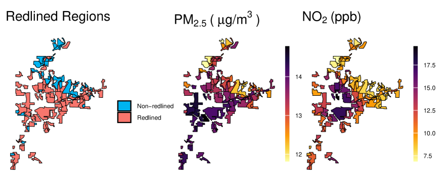
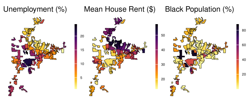
Figure 1: Data for Atlanta, GA. The first row shows the maps of redlined regions and non-redlined regions, and PM_2.5 and NO₂ levels. Second row shows unemployment rate, mean (monthly) house rent, and percent of Black population.

There is a substantial time gap between the redlining era (1935-1974) and the 2010 air pollution data. This introduces challenges such as potential attenuation of the redlining effects on air quality over time. Additionally, it complicates the identification and acquisition of confounders, particularly socio-economic status, which is a critical but debated concept among social scientists. To address this, we use data from the 1940 Census, including unemployment rates, housing conditions, and racial composition, as proxies for the underlying socio-economic status construct.

3 Statistical methods

The data are drawn from $M$ cities. City $i$ is partitioned into $N_{i}$ regions. For region $j\in\{1,\ldots,N_{i}\}$ in city $i$, the observed outcome, binary treatment, and $p$ proxy variables are denoted by $Y_{ij}\in\mathcal{R}$, $A_{ij}\in\{0,1\}$, and $\mbox{\bf W}_{ij}=(W_{ij1},\ldots,W_{ijp})^{\top}\in\mathcal{R}^{p}$. We posit two latent processes to capture confounding. The first is a non-spatial latent confounder process $\mbox{\bf U}_{ij}=(U_{ij1},\ldots,U_{ijq})^{\top}\in\mathcal{R}^{q}$, which accounts for unobserved factors influencing both treatment and outcome. The second is a spatial process $Z_{ij}\in\mathcal{R}$, which explains dependence in the outcome $Y_{ij}$ for nearby regions. Consider the model

$$Y_{ij} = \alpha_{y}+\theta A_{ij}+\bm{\alpha}_{yu}^{\top}\mbox{\bf U}_{ij}+\alpha_{yz}Z_{ij}+\epsilon_{y,ij},$$ (1)

$$A_{ij} = \text{I}(\alpha_{a}+\bm{\alpha}_{au}^{\top}\mbox{\bf U}_{ij}+\alpha_{az}Z_{ij}+\epsilon_{a,ij}>0),$$ (2)

$$\mbox{\bf W}_{ij} = \bm{\alpha}_{w}+\bm{\alpha}_{wu}\mbox{\bf U}_{ij}+\bm{\epsilon}_{w,ij},$$ (3)

where the error terms $\epsilon_{y,ij}$, $\epsilon_{a,ij}$, and $\bm{\epsilon}_{w,ij}$ are independent and identically distributed with mean zero and variances $\sigma_{y}^{2}$, $\sigma_{a}^{2}$, and $\bm{\Sigma}_{w}=\text{diag}(\sigma_{w_{1}}^{2},\ldots,\sigma_{w_{p}}^{2})$, respectively. Vectors $\bm{\alpha}_{au}$ and $\bm{\alpha}_{yu}$, both of length $q$, represent the coefficients for the relationships between the latent confounder $\mbox{\bf U}_{ij}$ and the treatment $A_{ij}$, and between $\mbox{\bf U}_{ij}$ and the outcome $Y_{ij}$, respectively. The matrix $\bm{\alpha}_{wu}$ is of dimension $p\times q$, representing the coefficients for the relationships between the proxy variables $\mbox{\bf W}_{ij}$ and the latent confounders $\mbox{\bf U}_{ij}$. Scalars $\alpha_{az}$ and $\alpha_{yz}$ represent the coefficients between the spatial process $Z_{ij}$ and the treatment $A_{ij}$, and between $Z_{ij}$ and the outcome $Y_{ij}$, respectively. The scalar $\theta$ is the treatment effect we aim to identify and estimate. Intercept terms include the vector $\bm{\alpha}_{w}$ and scalars $\alpha_{a}$ and $\alpha_{y}$.

With this design, we acknowledge the presence of latent confounders $\mbox{\bf U}_{ij}$ that can be captured through proxy variables $\mbox{\bf W}_{ij}$, and account for potential spatial confounding through the shared spatial process $Z_{ij}$. The latent confounder process variables $\mbox{\bf U}_{ij}$ are as

$$\mbox{\bf U}_{ij}\sim\mathcal{D}_{u}(\bm{\mu}_{u},\bm{\Sigma}_{u}),\quad\bm{\Sigma}_{u}=\text{diag}(\sigma_{u_{1}}^{2},\ldots,\sigma_{u_{q}}^{2}),$$ (4)

where $\mathcal{D}_{u}(\cdot)$ means arbitrary distribution with mean and finite variance; without loss of generality, the mean $\bm{\mu}_{u}$ can be set zero. The spatial latent variables are modeled using splines

$$Z_{ij}=\sum_{l=1}^{L_{i}}\lambda_{il}B_{ijl},\quad\lambda_{il}\sim\mathcal{D}_{\lambda}(0,\sigma_{z}^{2}),$$ (5)

where $\mathcal{D}_{\lambda}(\cdot)$ means arbitrary distribution with mean and finite variance; $B_{ijl}$ denotes the $l$-th spline basis function integrated over regions $j$ in city $i$ (see Section 5), and $\lambda_{il}$ are the corresponding coefficients.

4 Theoretical properties

We follow the potential outcomes framework (Rubin, 1976) and denote binary treatment as $A$ and outcome as $Y$, then the potential outcomes given a treatment is $Y(A)$. We are interested in the average treatment effect ATE $=\mathbb{E}(\sum_{i=1}^{M}\sum_{j=1}^{N_{j}}\big{\{}Y_{ij}(1)-Y_{ij}(0)\big{\}}/(M\sum_{i=1}^{M}N_{i}))$. With appropriate assumptions, we show that $\theta$ in Equation (1) is the ATE and we can directly use $\hat{\theta}$ as an ATE estimator.

Assumption 1 (SUTVA; Stable Unit Treatment Value Assumption).

(1) the potential outcomes for any unit does not vary with the treatment assigned to other units; (2) for each unit, there are no different versions of each treatment level that lead to different potential outcomes.

Assumption 2 (Latent Ignorability).

$A_{ij}\rotatebox[origin={c}]{90.0}{$\models$}Y_{ij}(a)|\mbox{\bf U}_{ij},Z_{ij}$ for any $a$. In other words, $\mbox{\bf U}_{ij}$ and $Z_{ij}$ account for all confounders influencing treatment and outcome.

Assumption 3 (Latent Positivity).

$P(A_{ij}=a|\mbox{\bf U}_{ij},Z_{ij})>0$ for any $a\in\{0,1\}$. That is, every unit has a non-zero probability of being assigned any treatment value.

Assumption 4 (Structural Causal Model).

The data-generating process is as specified in Equations (1) - (5). The indicator function $I(\cdot)$ in Equation (2) can be relaxed. In addition, we assume the two latent process are independent $Z_{ij}\rotatebox[origin={c}]{90.0}{$\models$}\mbox{\bf U}_{ij}$.

Assumption 5 (Sufficient Condition for Factor Model).

Let $\bm{\Lambda}=\bm{\alpha}_{wu}\bm{\Sigma}_{u|a}^{1/2}$, where $\bm{\Sigma}_{u|a}$ represents the conditional variance of $\mbox{\bf U}_{ij}$ given treatment $A_{ij}=a$. If any row of $\bm{\Lambda}$ is deleted, there remain two disjoint submatrices of rank $q$.

Our results also apply to continuous treatments, with modifications to Assumptions 3 and 5. These continuous counterparts are:

Assumption 3'. $P(A_{ij}=a|\mbox{\bf U}_{ij},Z_{ij})>0$ for any $a\in\mathcal{R}$.

Assumption 5'. Let $\bm{\Lambda}=\bm{\alpha}_{wu}\bm{\Sigma}_{u}^{1/2}$. If any row of $\bm{\Lambda}$ is deleted, there remain two disjoint submatrices of rank $q$.

Theorem 1.

Under Assumptions (1) - (5), or by replacing Assumptions (3) and (5) with their continuous counterparts (3') and (5'), the causal effect $\theta$ is identifiable.

We discuss identifiability of model parameters in two scenarios, when the treatment is continuous and binary, respectively. When the treatment is binary, we obtain (derivations in Appendix A.2)

$$\text{Cov}(\mbox{\bf W}_{ij}|A_{ij})=\bm{\alpha}_{wu}\bm{\Sigma}_{u|a}\bm{\alpha}_{wu}^{\top}+\bm{\Sigma}_{w},$$ (6)

$$\text{Cov}(\mbox{\bf W}_{ij},Y_{ij}|A_{ij})=\bm{\alpha}_{wu}\bm{\Sigma}_{u|a}\bm{\alpha}_{yu},$$ (7)

$$E(\mbox{\bf W}_{ij}|A_{ij})=\alpha_{a}+\bm{\alpha}_{wu}E(\mbox{\bf U}_{ij}|A_{ij}),$$ (8)

$$E(Y_{ij}|A_{ij})=\theta A_{ij}+\bm{\alpha}_{yu}E(\mbox{\bf U}_{ij}|A_{ij}).$$ (9)

In Equation (6), let $\bm{\Lambda}=\bm{\alpha}_{wu}\bm{\Sigma}_{u|a}^{1/2}$ of shape $p\times q$. We add Assumption 5, which is a strong and sufficient condition and implies $p\geq 2q+1$. With Assumption 5 and by applying Lemma 5.1 and Theorem 5.1 of Anderson and Rubin (1956), then $\bm{\Lambda}$ is identified up to rotations from the right under certain sufficient conditions. Specifically, $\bm{\alpha}_{wu}\bm{\Sigma}_{u|a}^{1/2}$ is identified up to multiplication on the right by an orthogonal matrix $\mbox{\bf R}_{1}$, so any admissible value for $\bm{\Lambda}$ can be written as $\bm{\Lambda}^{*}=\bm{\Lambda}\mbox{\bf R}_{1}$ with an arbitrary orthogonal matrix $\mbox{\bf R}_{1}$ of shape $q\times q$ (Miao et al. (2023), Kang et al. (2023)).

Plugging $\bm{\Lambda}$ into Equation (7), it becomes a linear system with $p$ equations and $q$ unknowns. $\bm{\Sigma}_{u|a}^{1/2}\bm{\alpha}_{yu}$ is identified up to multiplication on the left by $\mbox{\bf R}_{1}^{\top}$. Similarly, plugging $\bm{\Lambda}$ into Equation (8), then $E(\mbox{\bf U}_{ij}|A_{ij})$ is identified up to multiplication on the left by $\mbox{\bf R}_{1}^{\top}\bm{\Sigma}^{-1/2}_{u|a}$. Finally in Equation (9), $\bm{\alpha}_{yu}^{\top}E(\mbox{\bf U}_{ij}|A_{ij})$ has been identified since it can be expressed by $(\bm{\alpha}_{yu}^{\top}\bm{\Sigma}_{u|a}^{1/2}\mbox{\bf R}_{1})(\mbox{\bf R}_{1}^{\top}\bm{\Sigma}_{u|a}^{-1/2}E(\mbox{\bf U}_{ij}|A_{ij}))$, which are two components that have been identified. Consequently, the causal effect $\theta$ in Equation (9) can be uniquely identified. When spatial confounding $Z$ exists, we approximate it by B-splines (see details in Section 5.1). Equation (7) and (9) will be updated as below, while the method proof and conclusion remain the same.

$$\text{Cov}(\mbox{\bf W}_{ij},Y_{ij}|A_{ij})=\bm{\alpha}_{wu}\bm{\Sigma}_{u|a}\bm{\alpha}_{yu}+\text{Cov}(\mbox{\bf W}_{ij},Z_{ij}|A_{ij})\alpha_{yz},$$

$$E(Y_{ij}|A_{ij})=\theta A_{ij}+\bm{\alpha}_{yu}E(\mbox{\bf U}_{ij}|A_{ij})+\alpha_{yz}E(Z_{ij}|A_{ij}).$$

When the treatment is continuous, we obtain (derivations in Appendix A.2)

$$\text{cov}(\mbox{\bf W}_{ij})=\bm{\alpha}_{wu}\bm{\Sigma}_{u}\bm{\alpha}_{wu}^{\top}+\bm{\Sigma}_{w},$$ (10)

$$\text{cov}(\mbox{\bf W}_{ij},Y_{ij})=\text{cov}(\mbox{\bf W}_{ij},A_{ij})\theta+\bm{\alpha}_{wu}\bm{\Sigma}_{u}\bm{\alpha}_{yu}.$$ (11)

In Equation (10), let $\bm{\Lambda}=\bm{\alpha}_{wu}\bm{\Sigma}_{u}^{1/2}$ of shape $p\times q$. We add Assumption 5', then by applying Lemma 5.1 and Theorem 5.1 of Anderson and Rubin (1956), $\bm{\Lambda}$ is identified up to multiplication on the right by orthogonal matrix R. In Equation (11), denote $\bm{\Xi}=\bm{\Sigma}_{u}^{1/2}\bm{\alpha}_{yu}$, resulting in a linear system with $p$ equations and $(1+q)$ unknowns of $\theta$ and $\bm{\Xi}$. With the same Lemma 5.1 and Theorem 5.1 by Anderson and Rubin (1956), $p\geq 2q+1$ holds, therefore, these equations are over-determined and can be solved uniquely for $\theta$ using $\text{cov}(\mbox{\bf W}_{ij},Y_{ij})=\text{cov}(\mbox{\bf W}_{ij},A_{ij})\theta+\bm{\Lambda}^{*}\bm{\Xi}$.

5 Computational details

5.1 Approximation of spatial confounders

We assume an independent spatial latent process for each city and follow the estimation strategy of Dupont et al. (2022). We approximate spatial confounding $Z_{ij}$ by a linear combination of B-splines, $Z_{ij}=\sum_{l=1}^{L_{i}}\lambda_{il}B_{ijl}$, where $B_{ijl}$ is the $l$-th pre-computed spline basis function for region $j$ of city $i$ and $\lambda_{il}$ is the corresponding coefficient. The number of basis function is taken to be $L_{i}=\lfloor rN_{i}\rfloor$ where $r$ is the ratio of the number of basis functions to the number of regions in a city. The ratio $r$ is selected by minimizing Watanabe-Akaike Information Criterion (WAIC) of the outcome model (Gelman et al., 2014).

To create spline basis functions for city $i$, we define the minimum bounding rectangle $\mathcal{G}_{i}$ that encompasses city $i$, and place a 100-by-100 grid of points within $\mathcal{G}_{i}$, denoted by coordinates $\bm{s}_{k}$ for $k=\{1,2,...,10000\}$. Then we construct 2D cubic splines using this coordinates, denoted $b_{il}(\bm{s})$ for $l=\{1,...,L_{i}\}$. Finally, within polygon $A_{ij}$, we integrate these splines over locations $\bm{s}_{k}\in A_{ij}$, resulting in the spline basis $B_{ijl}=\sum_{k}b_{il}(\bm{s}_{k})\textbf{1}(\bm{s}_{k}\in A_{ij})/\sum_{k}\textbf{1}(\bm{s}_{k}\in A_{ij})$.

5.2 Bayesian Markov Chain Monte Carlo

We use Bayesian methods to incorporate uncertainties and address the inherent challenges in the complex data structure, including spatial and non-spatial latent variables, and zero-inflated proxies. We use a Markov chain Monte Carlo (MCMC) approach to sample from the joint posterior distribution of our model. Standard techniques for MCMC are employed, and uninformative priors are used when necessary.

For simulation studies, we run single chain MCMC with 50,000 burn-in iterations and 50,000 iterations post burn-in, with a thinning factor of 10. For real data analysis, we run single chain MCMC with 150,000 burn-in iterations and 150,000 more post burn-in, with a thinning factor of 10. Convergence is monitored using trace plots. Further details are provided in Appendix A.3.

6 Simulation study

The objectives of the simulation study are to evaluate the performance of our model in terms of estimation and inference. We conduct the simulation using two settings: (1) creating data with simple grid geometry and predetermined parameters, and (2) creating data that closely resemble the redlining data. For each parameter setting, we randomly generate 100 datasets.

6.1 Data generation

To create data with simple grid geometry and predetermined parameters, we generate 490 regions in 10 cities, consisting of 7-by-7 grid regions in each city. The data-generation process is defined by

$$U_{ij}\sim\mathcal{N}(0,1),\quad Z_{ij}=\sum_{l=1}^{L_{i}}\lambda_{il}B_{ijl},\quad\lambda_{il}\sim\mathcal{N}(0,1),$$

$$W_{ij1}\sim\mathcal{N}(\alpha_{w_{1}u}U_{ij},\sigma^{2}_{w_{1}}),\quad W_{ij2}\sim\mathcal{N}(\alpha_{w_{2}u}U_{ij},\sigma^{2}_{w_{2}}),$$

$$\tilde{W}_{ij3}\sim\mathcal{N}(\alpha_{w_{3}u}U_{ij},\sigma^{2}_{w_{3}}),\quad W_{ij3}=\max(\tilde{W}_{ij3},\text{quantile}_{.05}(\tilde{W}_{3})),$$

$$\text{logit}(P(A_{ij}=1))=\alpha_{a}+\alpha_{au}U_{ij}+\alpha_{az}Z_{ij},$$

$$Y_{ij}\sim\mathcal{N}(\theta A_{ij}+\alpha_{yu}U_{ij}+\alpha_{yz}Z_{ij},\sigma^{2}_{y}).$$

We consider four cases. The first is a base case with (1) $\theta=0.2$, $\alpha_{w_{1}u}=2$, $\alpha_{w_{2}u}=-0.5$, $\alpha_{w_{3}u}=-1$, $\sigma^{2}_{w_{1}}=\sigma^{2}_{w_{2}}=\sigma^{2}_{w_{3}}=1$, $r=40\%$, $\alpha_{a}=-1$, $\alpha_{au}=-1$, $\alpha_{az}=1$, $\alpha_{yu}=-0.2$, $\alpha_{yz}=-1$, $\sigma^{2}_{y}=0.25$. The others cases modify the base case as follows: (2) Stronger proxy: $\sigma^{2}_{w_{1}}=\sigma^{2}_{w_{2}}=\sigma^{2}_{w_{3}}=0.5$, (3) Noisier outcome: $\sigma^{2}_{y}=1$, and (4) Rougher spatial confounding: $r=60\%$. In all cases, $W_{ij3}$ is generated to have the lowest 5% percent values as zero, to model the zero-inflated percentage of Black Population in the real data.

To generate data that closely resemble the redlining data, we use the geometry of the redlining data. For each dataset, we take a random subset cities from the real data such that there are at least 500 regions in a dataset. We define true parameters as the posterior parameter estimates from real Redlining data analysis (using $r=60\%$). There are two cases: (a) outcome of NO₂, (b) outcome of PM_2.5.

6.2 Competing methods and metrics

We compare our method with two alternatives: (1) No adjustment for latent SES, removing latent process $\mbox{\bf U}_{ij}$ and proxy $\mbox{\bf W}_{ij}$ from the model; (2) Outcome Regression with Proxy, removing $\mbox{\bf U}_{ij}$ and moving proxy $\mbox{\bf W}_{ij}$ into the outcome regression as covariates. Both methods contains the spatial latent process $Z_{ij}$. We run models using spline ratios $r=\{0\%,20\%,40\%,60\%,80\%\}$ to explore a broad range of complexities in the spatial latent processes, and select the best model based on WAIC.

We denote the true effect as $\theta^{*}$. For each method, we denote the effect estimates as $\hat{\theta}_{t}$ for simulation data set $t$, $t\in\{1,...,100\}$, and $(L_{t},U_{t})$ as the corresponding credible intervals. We compute the following statistics: absolute bias $=100^{-1}|\sum_{t=1}^{100}(\hat{\theta}_{t}-\theta^{*})|$, mean squared error (MSE) $=100^{-1}\sum_{t=1}^{100}(\hat{\theta}_{t}-\theta^{*})^{2}$, and coverage probability $=100^{-1}\sum_{t=1}^{100}\mathbb{I}(\theta^{*}\in[L_{t},U_{t}])$.

6.3 Results

The simulation results are shown in Table 2, including the absolute bias (A.B.), mean squared error (MSE), coverage probability (%, C.P.), WAIC optimized over $r$, and the spline ratio (S.R.), each averaged over 100 simulations. Cases (1) - (4) use fully synthetic data, and cases (a) and (b) closely mimics the redlining data. In cases (1)-(4), our method obtains a satisfying coverage probability and negligible absolute bias and MSE. By minimizing WAIC, on average our method selects a spline ratio $r$ that is only slightly higher than the true ratio. In cases (a) and (b), the coverage probability is $90\%$ for NO₂ and $91\%$ for PM_2.5. Comparing across methods, our approach consistently produces coverage probabilities closest to the nominal 95% level, along with the lowest absolute bias and MSE. In summary, our method outperforms the alternatives across all evaluated metrics and simulation scenarios in Table 2. For additional robustness checks, we provide further simulations in Appendix A.4. These simulations explore scenarios with weaker proxies, stronger confounding, and spatial latent misspecification. The results demonstrate that our method remains robust when handling spatial structure. However, we observe minor performance drops in cases of weak proxies and strong confounding, which could be mitigated by adjusting the spline ratio.

Case	Method	A.B.	MSE	C.P.	WAIC	S.R.
(1)	Latent Adjustment	0.003 (0.106)	0.011 (0.015)	95	1083	54
	Outcome Regr with Proxy	0.245 (0.088)	0.068 (0.043)	18	1115	44
	No Adjustment	1.197 (0.106)	1.445 (0.257)	0	1460	42
(2)	Latent Adjustment	0.003 (0.086)	0.007 (0.010)	94	1030	49
	Outcome Regr with Proxy	0.135 (0.078)	0.024 (0.022)	55	1038	44
	No Adjustment	1.198 (0.102)	1.446 (0.246)	0	1460	42
(3)	Latent Adjustment	0.010 (0.159)	0.025 (0.040)	95	1590	43
	Outcome Regr with Proxy	0.228 (0.125)	0.067 (0.060)	54	1580	37
	No Adjustment	1.170 (0.143)	1.388 (0.341)	0	1736	40
(4)	Latent Adjustment	0.012 (0.107)	0.011 (0.014)	95	110	66
	Outcome Regr with Proxy	0.243 (0.090)	0.067 (0.041)	19	1144	58
	No Adjustment	1.198 (0.103)	1.445 (0.249)	0	1485	60
(a)	Latent Adjustment	0.001 (0.154)	0.023 (0.036)	90	1874	69
	Outcome Regr with Proxy	0.051 (0.215)	0.052 (0.079)	78	1905	68
	No Adjustment	0.640 (0.124)	0.425 (0.158)	0	1967	69
(b)	Latent Adjustment	0.003 (0.040)	0.002 (0.002)	91	470	69
	Outcome Regr with Proxy	0.004 (0.063)	0.004 (0.005)	73	498	68
	No Adjustment	0.048 (0.032)	0.003 (0.003)	67	478	68

Table 2: Simulation results by cases: (1) base case, (2) stronger proxy, (3) noisier outcome, (4) rougher spatial confounding, (a) use posterior parameters and outcome is NO₂, (b) use posterior parameters and outcome is PM_2.5. In case (1), (2), (3), the true spline ratio is 40%; in case (4), (a), (b), the true spline ratio is 60%. The columns display the average absolute bias (A.B.) with standard deviation, mean square error (MSE) with standard deviation, coverage probability (C.P.), Watanabe-Akaike Information Criterion (WAIC), and the selected spline ratio (S.R.).

7 Redlining policy analysis

We apply our method to study the effect of redlining policy on air pollution exposure. To account for socio-economic status in the 1930s, we define three proxy variables: the box-cox transformed unemployment rate, the mean house rent, and the rank-based inverse normal transformed percent of Black population. The treatment group is the relined group ($A=1$), and the control group is the non-redlined group ($A=0$). The outcomes are PM_2.5 and NO₂ levels in 2010, and we fit our model separately for each pollutant. All proxy variables and outcomes are centered by their mean per city before fitting the model.

In addition to the constant causal effect model discussed in Section 3, we also develop a random effect model, assuming that causal effects vary by city and are independent and identically distributed. Denote the city-level random effects as $\theta_{1},\ldots,\theta_{M}$. The outcome model in Equation (1) is then modified by replacing the constant $\theta$ with these city-specific random effects. Further details on both the constant and random effect models can be found in Appendix A.3.

7.1 Results

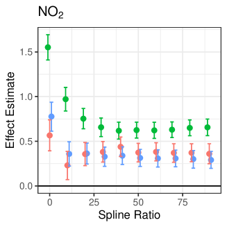
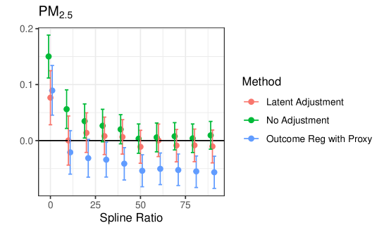
Figure 2: Redlining effect estimates and 95% credible intervals. The left panel shows results for NO₂ (ppb) and the right panel for PM_2.5 ($\mu$g/m³).

Figure 2 shows the posterior distribution of the long-term effects of redlining policies on air pollution exposure. The estimates stabilize as the spline ratio increases to a value large enough, whichever method being used. After adjusting for unmeasured confounding, our method indicate a significant effect for NO₂ and a non-significant effect for PM_2.5, as shown in Figure 2. At $r=60\%$, the estimated effect is 0.38 ppb (95% CI, 0.28 to 0.48) for NO₂ and 0.00 $\mu$g/m³ (95% CI, -0.03 to 0.03) for PM_2.5. This is very different from the raw difference between the treatment and control group, which is 2.48 ppb for NO₂ and 0.26 $\mu$g/m³ for PM_2.5.

For NO₂, the difference between Latent Adjustment and the Outcome Regression with Proxy is relatively minor, and they are both far from the No Adjustment. If our model correctly represents the data-generating process, then failing to adjust for unmeasured confounding leads to overestimation of the effect of NO₂. For PM_2.5, there is a clear difference between Latent Adjustment and Outcome Regression with Proxy. Assuming our model accurately represents the data-generating process, this discrepancy can be attributed to attenuation bias, biasing the effect estimate towards negative.

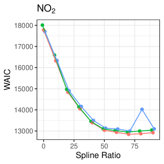
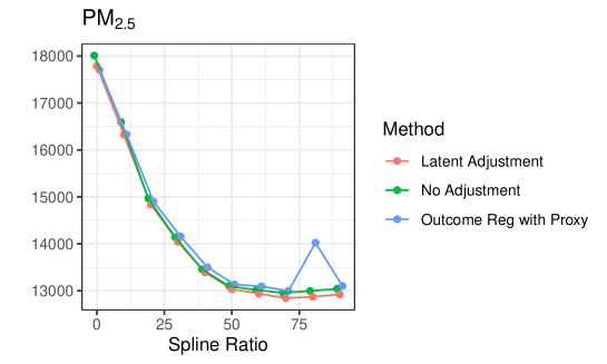
Figure 8: WAIC of outcome models for redlining real data analysis. The left panel for NO₂ and right for PM_2.5. The x-axis is the spline ratio $r$ and y-axis is WAIC. These plots demonstrate that the Latent Adjustment achieves the lowest WAIC values compared to the No Adjustment and Outcome Regression with Proxy methods for a wide ranges of spline ratio (50% to 90%). Additionally, all plots show a rapid decrease in WAIC values for the outcome models until $r$ reaches approximately 50%.

Appendix A.5, Figure 8 demonstrates that Latent Adjustment achieves lowest WAIC values compared to the No Adjustment and Outcome Regression with Proxy. There is a rapid decrease in WAIC values until spline ratio $r$ reaches approximately 60%. Given the stable estimates observed in Figure 2, we will highlight results at $r=60\%$ for the remainder of this paper.

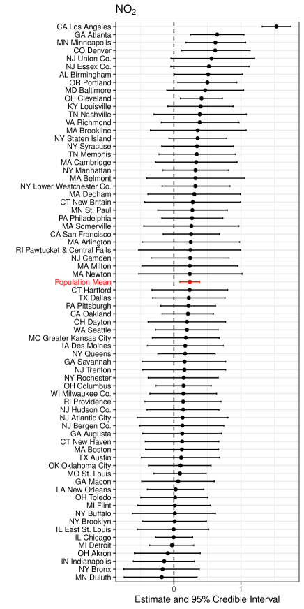
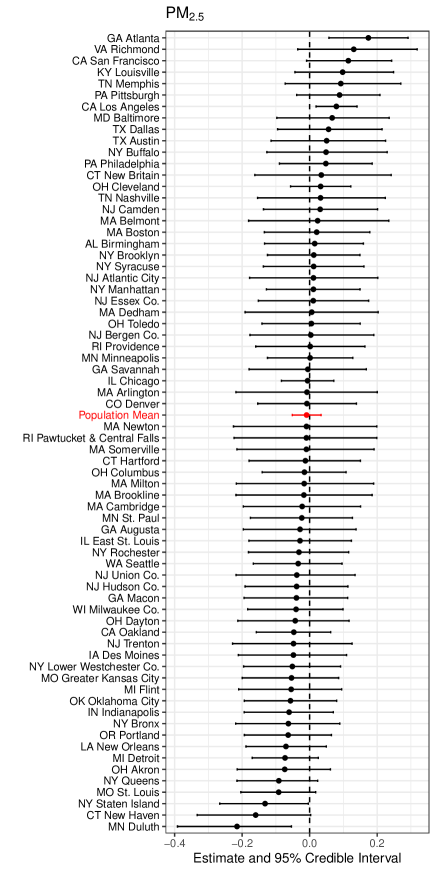
Figure 3: Posterior estimates of the long-term effects of redlining policies on NO₂ (left) and PM_2.5 (right) concentrations across 69 cities. Each city is represented by its posterior mean and 95% credible interval. The population mean is shown in red.

We apply a random effect model with $r=60\%$, where the results of the constant effects model had stabilized over a wide range of $r$ values. The population mean is 0.24 ppb (95% CI, 0.09 to 0.38) for NO₂ and -0.01 $\mu$g/m³ (95% CI, -0.05 to 0.03) for PM_2.5, which aligns with the constant effect model. As shown in Figure 3, for NO₂, seven out of 69 cities show strong evidence of a harmful effect (Los Angeles, CA; Minneapolis, MN; Denver, CO; Atlanta, GA; Birmingham, AL; Portland, OR; Cleveland, OH), while no cities show evidence of a protective effect. For PM_2.5, two cities show strong evidence of a harmful effect (Los Angeles, CA; Atlanta, GA), and two cities show strong evidence of a protective effect (Duluth, MN; Staten Island, NY). Notably, Los Angeles, CA and Atlanta, GA show strong evidence of harmful effects for both PM_2.5 and NO₂, with the strongest effects among the 69 cities studied.

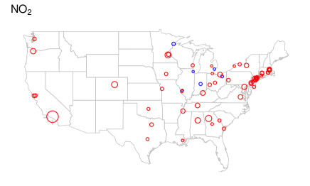
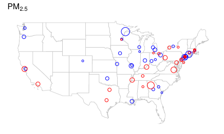
Figure 4: Mapping posterior estimates of the random effects across 69 cities. Harmful effects are represented by red dots and protective effects by blue dots, regardless of significance. Dot size is scaled by the absolute value of the effects.

The spatial distribution of the long-term effects across 69 cities, as depicted in Figure 4, reveals distinct geographic patterns. For PM_2.5, the harmful effects, indicated by red dots, are predominantly concentrated along the East Coast and in certain Midwestern and Western cities. Conversely, protective effects, represented by blue dots, are more apparent in central and northern cities. The relationship between these spatial patterns and urban development and population trends warrants further investigation. For NO₂, the spatial distribution of harmful effects is much broader, encompassing a wide range of geographic regions.

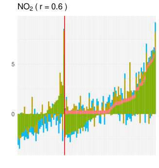
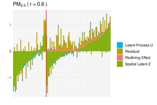
Figure 5: Sample results for Atlanta, GA, showing the decomposition of NO₂ (left) and PM_2.5 (right) across regions, when fitting with a random effect model with $r=60\%$. The x-axis represents the regions, and the y-axis shows the variance of PM_2.5 or NO₂. The red vertical bar separates the control group (regions on the left) from the treated group (regions on the right). The colors represent the posterior means of different components explaining the variance: Latent U (blue), Residual (brown), Redlining Effect (red), and Spatial Adjustment (green).

To provide an intuitive understanding of the results, Figure 5 presents the decomposition results for PM_2.5 and NO₂ across regions in Atlanta, GA, when fitting with a random effect model with $r=60\%$. The x-axis represents the regions, and the y-axis shows the values of NO₂ or PM_2.5. The red vertical bar separates the control group (regions on the left) from the treated group (regions on the right). The colors represent the posterior means of different components: Latent $U_{ij}$ (blue), Redlining Effect $\theta$ (red), Spatial Adjustment $Z_{ij}$ (green), and Residuals (brown). We observe a stronger confounding effect in NO₂ compared with PM_2.5. In both cases, spatial splines explain the majority of the variance in PM_2.5 and NO₂, which aligns with intuition as shown in Figure 1.

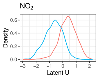
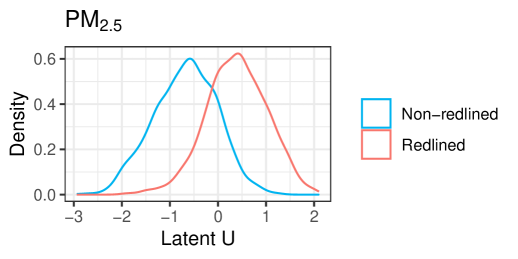
Figure 7: Overlap of latent $U_{ij}$ in the redlining data analysis with $r=60\%$ for NO₂ (left) and PM_2.5 (right). These density plots confirm that the overlap assumption is met, ensuring that there is sufficient overlap between the treatment and control groups for valid causal inference.

In Appendix A.5 Figure 4 and Figure 7, we confirm that the overlap and positivity assumptions are met, ensuring a solid foundation for causal inference. Appendix A.5 Table 5 demonstrates that we identify the latent $U_{ij}$ representing socio-economic status (SES) in the expected manner. A higher value in latent factor $U_{ij}$ indicates lower socio-economic status: $U_{ij}$ is associated with a higher unemployment rate, lower house rent, higher percentage of Black population, higher probability of being redlined, and higher air pollution levels.

8 Discussion

We estimate the long-term causal effects of redlining policies (1935-1974) on present-day NO₂ and PM_2.5 air pollution levels in 69 cities across 27 U.S. states. We found strong evidence of harmful effects of redlining policies on NO₂ concentrations, with an estimated effect of 0.38 ppb (95% CI, 0.28 to 0.48) even 36 years after the policy ended. We find no evidence of harmful effects on PM_2.5 concentrations after adjusting for unmeasured confounding, with an estimated effect of 0.00 $\mu$g/m³ (95% CI, -0.03 to 0.03). However, we can not dismiss the possibility that redlining once influenced PM_2.5 concentrations-an effect that may have diminished over time. These findings suggest that redlining has had a more pronounced impact on NO₂ levels.

NO₂ and PM_2.5 pollutants originate from different sources (US EPA (2023a), US EPA (2023b)). A potential explanation for the disparity in impacts between NO₂ and PM_2.5 may lie in highway vehicles, which is the primary contributor to NO₂. Highway vehicles could act as a mediating factor between redlining policies and NO₂ exposure levels.

To explore the variance of causal effects, we revise the model to include random effects. The population mean from the random effects model is 0.24 ppb (95% CI, 0.09 to 0.38) for NO₂ and -0.01 $\mu$g/m³ (95% CI, -0.05 to 0.03) for PM_2.5. For NO₂, most cities present harmful effects, although only a few are statistically significant. For PM_2.5, the harmful effects are predominantly concentrated along the East Coast and in certain Midwestern and Western cities. This pattern aligns well with the early urbanized areas of the 1930s and 1940s. Conversely, protective effects are more apparent in middle and northern cities, which largely urbanized during the Great Migration of the 1960s.

To our knowledge, this is the first study to investigate the causal effect of redlining policies on air pollution levels and one of the earliest to explore the causal effect of redlining policies on environmental risk exposure. The key strengths of this study are the following: (1) we conduct exhaustive adjustment for potential unmeasured confounding. We adjust for city-level confounders, spatial confounders using spatial splines, and confounder of socio-economic status using proxy variables. (2) We prove the identification of causal effect given the data generating process modeled. (3) We quantify uncertainty using Bayesian MCMC. (4) We conduct intensive simulation study to demonstrate the performance on estimation and inference of our method over other currently available bias correction methods.

Our study has several limitations in data and modeling. First, the air pollution data are not fully observed; they are derived from empirical models (Kim et al., 2020), and we do not account for this uncertainty. Second, our study covers only 69 cities. Historically, more cities were redlined (Nelson et al., 2023). The covered 69 cities might be the most urbanized, considering that they are covered in the 1940 U.S. census while others are not. This suggests that our study may not be representative of the entire redlined population.

Appendix A.1: Additional details of data cleaning

Our data cleaning process integrates multiple sources to create a coherent dataset for analysis.

Redlining Data: The Mapping Inequality Project has digitized the 1937 `residential security maps' created by the Home Owners' Loan Corporation (HOLC) (https://dsl.richmond.edu/panorama/redlining/data). This digitized data is invaluable for the redlining policy evaluation, particularly given the challenges of data collection in the 1930s due to technological limitations. We obtained the redlining data version in September 2022. This dataset includes digitized HOLC maps for 202 cities. To align with the 2010 census boundaries, we reformat these maps to match the 2010 census geography.

1940 Census Data: The 1940 census data is sourced from the National Historical Geographic Information System (NHGIS) (https://data2.nhgis.org/main). This dataset is selected because it is the closest census following the implementation of the redlining policies and offers a broader coverage of redlined cities compared to the 1930 census. In the web page, we select GEOGRAPHIC LEVELS as TRACT, YEARS as 1940, and downloaded the data with geographic boundaries based on the 2008 TIGER/Line files.

Unemployment rate is calculated as the ratio of the unemployed population to the total labor force. For home rent, the census data provides `gross monthly rent by homes' in categorical buckets ($<$$5, $5$-$$6, …, $75$-$$99, $100$+$). We use the midpoint of each category to compute a count-weighted mean home rent. The percentage of Black Population is the ratio of self-identified Black individuals to the total population.

Air Pollution Data: The raw PM_2.5 and NO₂ data for 2010 are retrieved from the Center for Air, Climate, and Energy Solutions (CACES).

Spatial Join and Missing Values: We merge these datasets using a spatial join method. For population counts, we assume an even spatial distribution and applied area-based weighting. Similarly, for rent and air pollution data, we use area weights to join these layers spatially. After the spatial join, we identify four regions with missing values for mean home rent. These are imputed using the average of the available non-missing values at the city level.

Data Representation: The original HOLC dataset contains 8,878 regions across 202 cities; 5,264 of the regions in 69 cities are fully or partially overlapped by the 1940 Census. We focus on 4,079 regions in these 69 cities that overlapped with both the 1940 census data and the 2010 air pollution data. Specifically, of all HOLC regions, 80.3% have at least 98% of their area covered by the 1940 census; 86.1% have at least 90% of their area covered by the 1940 census. This cleaned dataset captures approximately 25.5 million individuals, representing 20% of the 1940 U.S. population, thus providing a robust basis for our analysis.

Treatment and Control: In our analysis, we consider a binary treatment, labeling A and B as control group and C and D as treatment group. We make this decision for the reason that Redlining policies affected regions labeled as C and D more severely compared to A and B. According to Aaronson et al. (2021), Grade B was considered `like a 1935 automobile-still good, but not what the people are buying today who can afford a new one', whereas Grade C was becoming obsolete due to `expiring restrictions or lack of them' and `infiltration of a lower grade population'. HOLC field agents noted limited or no availability of mortgage funds in many `C' and `D' areas, such as parts of South, Southwest, and North Philadelphia (Hillier, 2003). This indicates that areas graded C and D faced more severe disinvestment and lending restrictions. By combining C and D into a single treatment group and A and B into a control group, we can make a clearer comparison of regions with different severities of redlining impacts.

Appendix A.2: Derivations

Binary treatment: Without loss of generality, we set intercepts $\bm{\alpha}_{w}=0,\alpha_{a}=0,\alpha_{y}=0$, and set $\bm{\mu}_{u}=0$ for latent factors. The models conditioning on the treatment can be formatted as below,

$$\left[\begin{array}[]{c}\mbox{\bf W}_{ij}\\ Y_{ij}\\ Z_{ij}\end{array}\right|\left.\begin{array}[]{c}\phantom{A_{ij}}\\ A_{ij}\\ \phantom{A}\end{array}\right]=\begin{bmatrix}\bm{\Gamma}&0&0\\ 0&0&\alpha_{yz}\\ 0&0&0\end{bmatrix}\left[\begin{array}[]{c}\mbox{\bf W}_{ij}\\ Y_{ij}\\ Z_{ij}\end{array}\right|\left.\begin{array}[]{c}\phantom{A_{ij}}\\ A_{ij}\\ \phantom{A}\end{array}\right]+\begin{bmatrix}\bm{\alpha}_{wu}\\ \bm{\alpha}_{yu}^{\top}\\ \bm{\alpha}_{zu|a}^{\top}\end{bmatrix}\left[\begin{array}[]{c}\mbox{\bf U}_{ij}\end{array}\right|\left.\begin{array}[]{c}A_{ij}\end{array}\right]+\begin{bmatrix}\bm{\epsilon}_{w}\\ \epsilon_{y}\\ \epsilon_{z}\end{bmatrix}$$ (26)

Let $\mbox{\bf B}=\begin{bmatrix}\bm{\Gamma}&0&0\\ 0&0&\alpha_{yz}\\ 0&0&0\end{bmatrix}$, then $(\mbox{\bf I}-\mbox{\bf B})^{-1}=\begin{bmatrix}\mbox{\bf I}-\bm{\Gamma}&0&0\\ 0&1&-\alpha_{yz}\\ 0&0&1\end{bmatrix}^{-1}=\begin{bmatrix}(\mbox{\bf I}-\bm{\Gamma})^{-1}&0&0\\ 0&1&\alpha_{yz}\\ 0&0&1\end{bmatrix}$

$$\text{Cov}\left[\begin{array}[]{c}\mbox{\bf W}_{ij}\\ Y_{ij}\\ Z_{ij}\end{array}\right|\left.\begin{array}[]{c}\phantom{A_{ij}}\\ A_{ij}\\ \phantom{A}\end{array}\right]$$

$$=\begin{bmatrix}(\mbox{\bf I}-\bm{\Gamma})^{-1}&0&0\\ 0&1&\alpha_{yz}\\ 0&0&1\end{bmatrix}\begin{bmatrix}(\bm{\alpha}_{wu}\bm{\Sigma}_{u|a}\bm{\alpha}_{wu}^{\top}+\bm{\Sigma}_{w})&\bm{\alpha}_{wu}\bm{\Sigma}_{u|a}\bm{\alpha}_{yu}&\bm{\alpha}_{wu}\bm{\Sigma}_{u|a}\bm{\alpha}_{zu|a}\\ \bm{\alpha}_{yu}^{\top}\bm{\Sigma}_{u|a}\bm{\alpha}_{wu}^{\top}&(\bm{\alpha}_{yu}^{\top}\bm{\Sigma}_{u|a}\bm{\alpha}_{yu}+\sigma^{2}_{y})&\bm{\alpha}_{yu}^{\top}\bm{\Sigma}_{u|a}\bm{\alpha}_{zu|a}\\ \bm{\alpha}_{zu|a}^{\top}\bm{\Sigma}_{u|a}\bm{\alpha}_{wu}^{\top}&\bm{\alpha}_{zu|a}^{\top}\bm{\Sigma}_{u|a}\bm{\alpha}_{yu}&(\bm{\alpha}_{zu|a}^{\top}\bm{\Sigma}_{u|a}\bm{\alpha}_{zu|a}+\Sigma_{z})\end{bmatrix}\begin{bmatrix}(\mbox{\bf I}-\bm{\Gamma})^{-1}&0&0\\ 0&1&\alpha_{yz}\\ 0&0&1\end{bmatrix}$$

$$=\begin{bmatrix}(\mbox{\bf I}-\bm{\Gamma})^{-1}(\bm{\alpha}_{wu}\bm{\Sigma}_{u|a}\bm{\alpha}_{wu}^{\top}+\bm{\Sigma}_{w})(\mbox{\bf I}-\bm{\Gamma})^{-1}&...&...\\ \bm{\alpha}_{yu}^{\top}\bm{\Sigma}_{u|a}\bm{\alpha}_{wu}^{\top}(\mbox{\bf I}-\bm{\Gamma})^{-1}+\bm{\alpha}_{zu|a}^{\top}\bm{\Sigma}_{u|a}\bm{\alpha}_{wu}^{\top}(\mbox{\bf I}-\bm{\Gamma})^{-1}\alpha_{yz}&(\bm{\alpha}_{yu}^{\top}\bm{\Sigma}_{u|a}\bm{\alpha}_{yu}+\sigma^{2}_{y})+(\bm{\alpha}_{zu|a}^{\top}\bm{\Sigma}_{u|a}\bm{\alpha}_{yu})\alpha_{yz}&...\\ (\bm{\alpha}_{zu|a}^{\top}\bm{\Sigma}_{u|a}\bm{\alpha}_{wu}^{\top})(\mbox{\bf I}-\bm{\Gamma})^{-1}&\bm{\alpha}_{zu|a}^{\top}\bm{\Sigma}_{u|a}\bm{\alpha}_{yu}&...+\Sigma_{z}\end{bmatrix}$$

When $\bm{\Gamma}$ is a zero matrix, we derive Equation (6) and (7). When $\Gamma$ is not zero matrix but known, the theorem still holds.

Continuous treatment: The equations in 1, 2, 3, 4 can be formatted as below, and `0' could be a scalar or vector.

$$\begin{bmatrix}\mbox{\bf W}_{ij}\\ A_{ij}\\ Y_{ij}\\ Z_{ij}\end{bmatrix}=\begin{bmatrix}\bm{\Gamma}&0&0&0\\ 0&0&0&\alpha_{az}\\ 0&\theta&0&\alpha_{yz}\\ 0&0&0&0\end{bmatrix}\begin{bmatrix}\mbox{\bf W}_{ij}\\ A_{ij}\\ Y_{ij}\\ Z_{ij}\end{bmatrix}+\begin{bmatrix}\bm{\alpha}_{wu}\\ \bm{\alpha}_{au}^{\top}\\ \bm{\alpha}_{yu}^{\top}\\ 0\end{bmatrix}\mbox{\bf U}_{ij}+\begin{bmatrix}\bm{\epsilon}_{w}\\ \epsilon_{a}\\ \epsilon_{y}\\ \epsilon_{z}\end{bmatrix}$$ (27)

where $\bm{\Gamma}$ is the auto-correlations between proxies, with zero on diagonal.

Let $\mbox{\bf B}=\begin{bmatrix}\bm{\Gamma}&0&0&0\\ 0&0&0&\alpha_{az}\\ 0&\theta&0&\alpha_{yz}\\ 0&0&0&0\end{bmatrix}$, then $(I-\mbox{\bf B})^{-1}=\begin{bmatrix}\mbox{\bf I}-\bm{\Gamma}&0&0&0\\ 0&1&0&-\alpha_{az}\\ 0&-\theta&1&-\alpha_{yz}\\ 0&0&0&1\end{bmatrix}^{-1}=\begin{bmatrix}(I-\bm{\Gamma})^{-1}&0&0&0\\ 0&1&0&\alpha_{az}\\ 0&\theta&1&\alpha_{az}\theta+\alpha_{yz}\\ 0&0&0&1\end{bmatrix}$

$$\text{Cov}\begin{bmatrix}\mbox{\bf W}_{ij}\\ A_{ij}\\ Y_{ij}\\ Z_{ij}\end{bmatrix}=\begin{bmatrix}(\mbox{\bf I}-\bm{\Gamma})^{-1}&0&0&0\\ 0&1&0&\alpha_{az}\\ 0&\theta&1&\alpha_{az}\theta+\alpha_{yz}\\ 0&0&0&1\end{bmatrix}$$

$$\hskip 28.45274pt\begin{bmatrix}(\bm{\alpha}_{wu}\bm{\Sigma}_{u}\bm{\alpha}_{wu}^{\top}+\bm{\Sigma}_{w})&\bm{\alpha}_{wu}\bm{\Sigma}_{u}\bm{\alpha}_{au}&\bm{\alpha}_{wu}\bm{\Sigma}_{u}\bm{\alpha}_{yu}&0\\ \bm{\alpha}_{au}^{\top}\bm{\Sigma}_{u}\bm{\alpha}_{wu}^{\top}&(\bm{\alpha}_{au}^{\top}\bm{\Sigma}_{u}\bm{\alpha}_{au}+\sigma^{2}_{a})&\bm{\alpha}_{au}^{\top}\bm{\Sigma}_{u}\bm{\alpha}_{yu}&0\\ \bm{\alpha}_{yu}^{\top}\bm{\Sigma}_{u}\bm{\alpha}_{wu}^{\top}&\bm{\alpha}_{yu}^{\top}\bm{\Sigma}_{u}\bm{\alpha}_{au}&(\bm{\alpha}_{yu}^{\top}\bm{\Sigma}_{u}\bm{\alpha}_{yu}+\sigma^{2}_{y})&0\\ 0&0&0&\Sigma_{z}\end{bmatrix}\begin{bmatrix}(\mbox{\bf I}-\bm{\Gamma})^{-1}&0&0&0\\ 0&1&\theta&0\\ 0&0&1&0\\ 0&\alpha_{az}&\alpha_{az}\theta+\alpha_{yz}&1\end{bmatrix}$$

$$=\begin{bmatrix}(\mbox{\bf I}-\bm{\Gamma})^{-1}(\bm{\alpha}_{wu}\bm{\Sigma}_{u}\bm{\alpha}_{wu}^{\top}+\bm{\Sigma}_{w})(\mbox{\bf I}-\bm{\Gamma})^{-1}&...&...&...\\ \bm{\alpha}_{au}^{\top}\bm{\Sigma}_{u}\bm{\alpha}_{wu}^{\top}(\mbox{\bf I}-\bm{\Gamma})^{-1}&(\bm{\alpha}_{au}^{\top}\bm{\Sigma}_{u}\bm{\alpha}_{au}+\sigma^{2}_{a})+\alpha_{az}\Sigma_{z}\alpha_{az}&...&...\\ (\theta\bm{\alpha}_{au}^{\top}\bm{\Sigma}_{u}\bm{\alpha}_{wu}^{\top}+\bm{\alpha}_{yu}^{\top}\bm{\Sigma}_{u}\bm{\alpha}_{wu}^{\top})(\mbox{\bf I}-\bm{\Gamma})^{-1}&\theta(\bm{\alpha}_{au}^{\top}\bm{\Sigma}_{u}\bm{\alpha}_{au}+\sigma^{2}_{a})+\bm{\alpha}_{yu}^{\top}\bm{\Sigma}_{u}\bm{\alpha}_{au}+(\alpha_{az}\theta+\alpha_{yz})\Sigma_{z}\alpha_{az}&...+\sigma_{y}^{2}&...\\ 0&\Sigma_{z}\alpha_{az}&\Sigma_{z}(\alpha_{az}\beta+\alpha_{yz})&\Sigma_{z}\end{bmatrix}$$

When $\bm{\Gamma}$ is a zero matrix, we derive Equation (10) and (11). When $\bm{\Gamma}$ is not zero matrix but known, the theorem still holds.

Appendix A.3: Computational details

Latent factor model: We use Metropolis-Hastings Sampling to update the latent process $\mbox{\bf U}_{ij}$ and $\lambda_{il}$ city-by-city. We use prior $\mbox{\bf U}_{ij}\stackrel{{\scriptstyle iid}}{{\sim}}\mathcal{N}(0,\text{diag}(\sigma_{u_{1}}^{2},...,\sigma_{u_{q}}^{2}))$ for any $i$ and $j$, $\lambda_{il}\stackrel{{\scriptstyle iid}}{{\sim}}\mathcal{N}(0,\sigma_{z}^{2})$ for any $i$ and $l$, and $\sigma_{u_{1}}^{2},...,\sigma_{u_{q}}^{2},\sigma_{z}^{2}\stackrel{{\scriptstyle iid}}{{\sim}}\text{InvGamma}(0.01,0.01)$. In practice, we set $\alpha_{w_{1}u}=1$ to scale $U_{ij1}$ by $W_{ij1}$.

Normally distributed proxy: We use Gibbs sampling for this standard regression model with parameters $\bm{\alpha}_{w},\bm{\alpha}_{wu},\sigma^{2}_{w_{1}},...,\sigma^{2}_{w_{p}}$. We use priors for each element of $\bm{\alpha}_{w},\bm{\alpha}_{wu}$ to be i.i.d. $\mathcal{N}(0,\tau_{w}^{2})$, and $\tau_{w}^{2},\sigma^{2}_{w_{1}}$ $,...,$ $\sigma^{2}_{w_{p}}\stackrel{{\scriptstyle iid}}{{\sim}}\text{InvGamma}(0.01,0.01)$.

Zero-inflated proxy: The variable percentage of Black population (denoted as $W_{ij1}$ for convenience in this paragraph) has around 5% values being zeros. We transform it by rank-based inverse normal and fit it with a zero-inflated Tobit model. Let $w_{L}$ denote the censoring boundary (meaning percent of Black population is zero). The evaluated likelihood function in city $i$ is:

$$\mathcal{L}(\cdot;W_{ij1},\mbox{\bf U}_{ij})=\prod^{i}\bigg{(}\frac{1}{\sigma_{w_{1}}}\phi\bigg{(}\frac{W_{ij1}-h(\mbox{\bf U}_{ij})}{\sigma_{w_{1}}}\bigg{)}\bigg{)}^{I(W_{ij1})}\prod^{i}\bigg{(}1-\Phi\bigg{(}\frac{h(\mbox{\bf U}_{ij})-w_{L}}{\sigma_{w_{1}}}\bigg{)}\bigg{)}^{1-I(W_{ij1})}$$

where $I(w)=\begin{cases}0,&w\leq w_{L}\\ 1,&w>w_{L}\end{cases}$; $\phi$ and $\Phi$ denote the density function and cumulative density function of the standard normal distribution, respectively; $h(\mbox{\bf U}_{ij})$ denotes the conditional expectation $h(\mbox{\bf U}_{ij})=\alpha_{w_{1}}+\bm{\alpha}_{w_{1}u}\mbox{\bf U}_{ij}$. We use Metropolis-Hastings sampling to update all parameters with a standard acceptance probability. We use priors $\alpha_{w_{1}},\bm{\alpha}_{w_{1}u}\stackrel{{\scriptstyle iid}}{{\sim}}\mathcal{N}(0,\tau_{w}^{2})$, and $\tau_{w_{1}}^{2},\sigma^{2}_{w_{1}}\sim\text{InvGamma}(0.01,0.01)$. The candidate of $\sigma^{2}_{w_{1}}$ is obtained from a log-normal distribution to ensure positivity.

Treatment model: The treatment model is modeled $\text{logit}(P(A_{ij}=1|\mbox{\bf U}_{ij},Z_{ij}))=\alpha_{a}+\bm{\alpha}_{au}\mbox{\bf U}_{ij}+\alpha_{az}Z_{ij}$. We use Metropolis-Hastings Sampling to update parameters $\alpha_{a},\bm{\alpha}_{au}$. We use priors for each element of $\alpha_{a},\bm{\alpha}_{au}\stackrel{{\scriptstyle iid}}{{\sim}}\mathcal{N}(0,\tau_{1}^{2})$, $\tau_{1}^{2}\sim\text{InvGamma}(0.01,0.01)$. We set $\alpha_{az}=1$ to scale the values of latent $Z_{ij}$.

Outcome model: The outcome model is $Y_{ij}|A_{ij},\mbox{\bf U}_{ij},Z_{ij}\sim\mathcal{N}(\alpha_{y}+\theta A_{ij}+\bm{\alpha}_{yu}\mbox{\bf U}_{ij}+\alpha_{yz}Z_{ij},\sigma^{2}_{y})$. We use Gibbs Sampling to update all involved parameters. We use priors $\alpha_{y},\theta,\bm{\alpha}_{yu}\sim\mathcal{N}(0,\tau_{2}^{2})$, $\alpha_{yz}\sim\mathcal{N}(0,\tau_{3}^{2})$, $\sigma^{2}_{y},\tau_{2}^{2},\tau_{3}^{2}\sim\text{InvGamma}(0.01,0.01)$.

Random effect model: Denote the city-level random effects $\theta_{1},\ldots,\theta_{M}\stackrel{{\scriptstyle iid}}{{\sim}}\mathcal{N}(\mu_{\theta},\sigma^{2}_{\theta})$. We use priors $\mu_{\theta}\sim\mathcal{N}(0,100^{2})$, $\sigma_{\theta}^{2}\sim\text{InvGamma}(0.01,0.01)$. This model uses the posterior parameter estimates from the constant effect model as initial values, which significantly speed up convergence.

Other Implementation Details: We fit the models via MCMC and obtained posterior samples of all the unknown parameters. The data and statistical models fit with R 4.2.3 have been made available with the paper. JABS/BUGS is not preferred due to computational efficiency.

Appendix A.4: Additional results for simulation study

We extended the simulation study by modifying the base case (1) to include three additional scenarios: case (5) Weaker proxy, where $\sigma^{2}_{w_{1}}=\sigma^{2}_{w_{2}}=\sigma^{2}_{w_{3}}=2$; (6) Stronger confounding $U$, where $\alpha_{au}=-2$, $\alpha_{yu}=-1$; (7) Misspecification with spatial latent, where $U_{ij}\sim\mathcal{N}(\sum_{l=1}^{L_{i}}\eta_{il}B_{il}(\mbox{\bf s}_{ij}),1)$, $\eta_{il}\sim\mathcal{N}(0,0.5)$. The results are shown in Table 3.

In all cases, the Latent Adjustment method consistently outperformed the alternative methods across all metrics. Specifically, in Case (7), the Latent Adjustment method achieved coverage probabilities to the nominal 95% level, demonstrating its robustness to spatial misspecification of the latent $U_{ij}$. However, Cases (5) and (6) showed a minor decline in performance, with increased positive bias and lower coverage probabilities. If the correct spline ratio of 60% had been used, the coverage probabilities for Cases (5) and (6) would have improved to 92% and 93%, respectively. That means, when the proxy $\mbox{\bf W}_{ij}$ is weak or the confounding effect of $U_{ij}$ is strong, challenges in model selection persist, leading to increased bias and reduced coverage probability.

Case	Method	A.B.	MSE	C.P.	WAIC	S.R.
(5)	Latent Adjustment	0.044 (0.166)	0.029 (0.043)	85	1087	59
	Outcome Regr with Proxy	0.412 (0.097)	0.179 (0.077)	2	1209	45
	No Adjustment	1.141 (0.080)	1.309 (0.177)	0	1482	35
(6)	Latent Adjustment	0.080 (0.178)	0.038 (0.058)	84	1093	60
	Outcome Regr with Proxy	0.485 (0.116)	0.248 (0.110)	1	1469	39
	No Adjustment	2.371 (0.196)	5.660 (0.934)	0	1992	35
(7)	Latent Adjustment	0.01 (0.097)	0.01 (0.012)	95	1094	54
	Outcome Regr with Proxy	0.26 (0.088)	0.08 (0.046)	13	1125	44
	No Adjustment	1.22 (0.106)	1.50 (0.264)	0	1465	43

Table 3: Simulation results by cases: (5) weaker proxy, (6) stronger confounder $U$, (7) spatial latent $U$. In all cases, the true spline ratio is 40%. The columns display the average absolute bias (A.B.) with standard deviation, mean square error (MSE) with standard deviation, coverage probability (%, C.P.), Watanabe-Akaike Information Criterion (WAIC), and the selected spline ratio (S.R.).

Appendix A.5: Additional results for redlining policy analysis

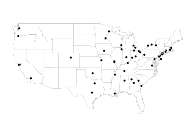
Figure 6: Map showing the distribution of 69 cities across 27 states included in our study.

Outcome	Q0	Q2.5	Q25	Q50	Q75	Q97.5	Q100
NO2	1.00	1.00	0.98	0.96	0.89	0.45	0.08
PM2.5	1.00	1.00	0.98	0.96	0.89	0.49	0.11

Table 4: Positivity of treatment assignment in the redlining data analysis with $r=60\%$. The values indicate the probability of being redlined for a given value of $U_{ij}$ at specific quantiles of the $U_{ij}$ distribution, controlling $Z_{ij}=0$. This table confirms that the positivity assumption is moderately met.

Outcome	Unemployment Rate	House Rent	Percent of Black	Probability of Being Redlined	Outcome
NO2	1.00	-0.93	0.19	1.86	0.71
PM2.5	1.00	-0.87	0.20	1.79	0.04

Table 5: Posterior estimates of parameters ($\alpha_{w_{1}u},\alpha_{w_{2}u},\alpha_{w_{3}u},\alpha_{au},\alpha_{yu}$) representing the relationship between the latent $U_{ij}$ and other variables in the redlining data analysis when $r=60\%$ . The values are comparable within columns but not across rows. The absolute values contains limited information, since the data are transformed, scaled, and centered. This table illustrates that, whether the outcome is PM_2.5 or NO₂, we consistently identify a latent factor $U_{ij}$ representing socio-economic status (SES) as expected: higher values of $U_{ij}$ correspond to lower SES and are numerically associated with higher unemployment rates, lower housing rent, a higher percentage of Black population, increased probability of being redlined, and elevated air pollution levels.

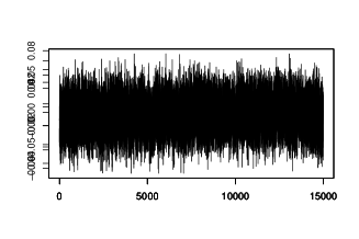
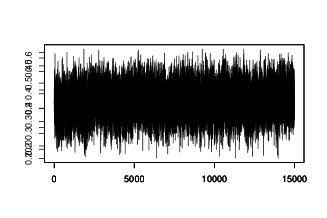
Figure 9: Example trace plot with 150,000 iterations after burn-in for relining data analysis. PM_2.5 is shown on the left, NO₂ on the right. Form top to bottom, the values of $r$ are 10%, 40%, 70%. he trace plots indicate stable convergence of multiple models.

References

- Aaronson et al. (2021) Aaronson, D., Hartley, D. and Mazumder, B. (2021) The effects of the 1930s HOLC “redlining” maps. American Economic Journal: Economic Policy, 13, 355–392.
- Anderson and Rubin (1956) Anderson, T. and Rubin, H. (1956) Statistical inference in factor analysis. In Proceedings of the Berkeley Symposium on Mathematical Statistics and Probability, 111. University of California Press.
- Bound et al. (1995) Bound, J., Jaeger, D. A. and Baker, R. M. (1995) Problems with instrumental variables estimation when the correlation between the instruments and the endogenous explanatory variable is weak. Journal of the American statistical association, 90, 443–450.
- Davis et al. (2021) Davis, M. L., Neelon, B., Nietert, P. J., Burgette, L. F., Hunt, K. J., Lawson, A. B. and Egede, L. E. (2021) Propensity score matching for multilevel spatial data: accounting for geographic confounding in health disparity studies. International Journal of Health Geographics, 20, 1–12.
- Davis et al. (2019) Davis, M. L., Neelon, B., Nietert, P. J., Hunt, K. J., Burgette, L. F., Lawson, A. B. and Egede, L. E. (2019) Addressing geographic confounding through spatial propensity scores: a study of racial disparities in diabetes. Statistical Methods in Medical Research, 28, 734–748.
- Dupont et al. (2022) Dupont, E., Wood, S. N. and Augustin, N. H. (2022) Spatial+: a novel approach to spatial confounding. Biometrics, 78, 1279–1290.
- Fishback et al. (2020) Fishback, P. V., LaVoice, J., Shertzer, A. and Walsh, R. (2020) The HOLC maps: How race and poverty influenced real estate professionals’ evaluation of lending risk in the 1930s. Tech. rep., National Bureau of Economic Research.
- Gelman et al. (2014) Gelman, A., Hwang, J. and Vehtari, A. (2014) Understanding predictive information criteria for Bayesian models. Statistics and computing, 24, 997–1016.
- Giffin et al. (2021) Giffin, A., Reich, B. J., Yang, S. and Rappold, A. G. (2021) Instrumental variables, spatial confounding and interference. arXiv preprint arXiv:2103.00304.
- Gilbert et al. (2021) Gilbert, B., Datta, A. and Ogburn, E. (2021) Approaches to spatial confounding in geostatistics. arXiv preprint arXiv: 2112.14946.
- Guan et al. (2023) Guan, Y., Page, G. L., Reich, B. J., Ventrucci, M. and Yang, S. (2023) Spectral adjustment for spatial confounding. Biometrika, 110, 699–719.
- Haschka et al. (2020) Haschka, R. E., Schley, K. and Herwartz, H. (2020) Provision of health care services and regional diversity in germany: Insights from a Bayesian health frontier analysis with spatial dependencies. The European Journal of Health Economics, 21, 55–71.
- Hillier (2003) Hillier, A. E. (2003) Redlining and the home owners' loan corporation. Journal of Urban History, 29, 394–420.
- Jerzak et al. (2023) Jerzak, C. T., Johansson, F. and Daoud, A. (2023) Integrating earth observation data into causal inference: challenges and opportunities. arXiv preprint arXiv:2301.12985.
- Jung et al. (2022) Jung, K. H., Pitkowsky, Z., Argenio, K., Quinn, J. W., Bruzzese, J.-M., Miller, R. L., Chillrud, S. N., Perzanowski, M., Stingone, J. A. and Lovinsky-Desir, S. (2022) The effects of the historical practice of residential redlining in the united states on recent temporal trends of air pollution near new york city schools. Environment International, 169, 107551.
- Kang et al. (2023) Kang, S., Franks, A. and Antonelli, J. (2023) Sensitivity analysis with multiple treatments and multiple outcomes with applications to air pollution mixtures. arXiv preprint arXiv:2311.12252.
- Kim et al. (2020) Kim, S.-Y., Bechle, M., Hankey, S., Sheppard, L., Szpiro, A. A. and Marshall, J. D. (2020) Concentrations of criteria pollutants in the contiguous us, 1979–2015: Role of prediction model parsimony in integrated empirical geographic regression. PloS one, 15, e0228535.
- Kong et al. (2019) Kong, D., Yang, S. and Wang, L. (2019) Multi-cause causal inference with unmeasured confounding and binary outcome. arXiv: Methodology.
- Kuroki and Pearl (2014) Kuroki, M. and Pearl, J. (2014) Measurement bias and effect restoration in causal inference. Biometrika, 101, 423–437.
- Lane et al. (2022) Lane, H. M., Morello-Frosch, R., Marshall, J. D. and Apte, J. S. (2022) Historical redlining is associated with present-day air pollution disparities in US cities. Environmental Science & Technology Letters, 9, 345–350.
- Lipsitch et al. (2010) Lipsitch, M., Tchetgen, E. T. and Cohen, T. (2010) Negative controls: a tool for detecting confounding and bias in observational studies. Epidemiology (Cambridge, Mass.), 21, 383.
- Miao et al. (2023) Miao, W., Hu, W., Ogburn, E. L. and Zhou, X.-H. (2023) Identifying effects of multiple treatments in the presence of unmeasured confounding. Journal of the American Statistical Association, 118, 1953–1967.
- Miao et al. (2018) Miao, W., Shi, X. and Tchetgen, E. T. (2018) A confounding bridge approach for double negative control inference on causal effects. arXiv preprint arXiv:1808.04945.
- Nelson et al. (2023) Nelson, R. K., Winling, L. and et al. (2023) Mapping inequality: Redlining in new deal america. https://dsl.richmond.edu/panorama/redlining. Digital Scholarship Lab, University of Richmond.
- Papadogeorgou et al. (2019) Papadogeorgou, G., Choirat, C. and Zigler, C. M. (2019) Adjusting for unmeasured spatial confounding with distance adjusted propensity score matching. Biostatistics, 20, 256–272.
- Reich et al. (2021) Reich, B. J., Yang, S., Guan, Y., Giffin, A. B., Miller, M. J. and Rappold, A. (2021) A review of spatial causal inference methods for environmental and epidemiological applications. International Statistical Review, 89, 605–634.
- Rubin (1976) Rubin, D. B. (1976) Inference and missing data. Biometrika, 63, 581–592.
- Schnell and Papadogeorgou (2020) Schnell, P. M. and Papadogeorgou, G. (2020) Mitigating unobserved spatial confounding when estimating the effect of supermarket access on cardiovascular disease deaths. arXiv preprint arXiv:1907.12150.
- Shao et al. (2022) Shao, R., Derudder, B. and Yang, Y. (2022) Metro accessibility and space-time flexibility of shopping travel: A propensity score matching analysis. Sustainable Cities and Society, 87, 104204.
- Tustin et al. (2017) Tustin, A. W., Hirsch, A. G., Rasmussen, S. G., Casey, J. A., Bandeen-Roche, K. and Schwartz, B. S. (2017) Associations between unconventional natural gas development and nasal and sinus, migraine headache, and fatigue symptoms in pennsylvania. Environmental Health Perspectives, 125, 189–197.
-
US EPA (2023a)
US EPA (2023a) Overview of Nitrogen Dioxide (NO2) Air Quality in the United States
https://www.epa.gov/system/files/documents/2023-06/NO2_2022.pdf. Accessed: 2024-08-22. -
US EPA (2023b)
— (2023b) Overview of Particulate Matter (PM) Air Quality in the United States
https://www.epa.gov/system/files/documents/2023-06/PM_2022.pdf. Accessed: 2024-08-22. -
US EPA (2024)
— (2024) Timeline of particulate matter (pm) national ambient air quality standards (naaqs)
https://www.epa.gov/pm-pollution/
timeline-particulate-matter-pm-national-ambient-air-quality
-standards-naaqs. Accessed: 2024-05-20. - Yang et al. (2020) Yang, S., Zeng, D. and Wang, X. (2020) Improved inference for heterogeneous treatment effects using real-world data subject to hidden confounding. arXiv preprint arXiv:2007.12922.