Rethinking the Win Ratio: A Causal Framework for Hierarchical Outcome Analysis

Abstract

Quantifying causal effects in the presence of complex and multivariate outcomes is a key challenge to evaluate treatment effects. For hierarchical multivarariates outcomes, the FDA recommends the Win Ratio and Generalized Pairwise Comparisons approaches Pocock et al. (2011); Buyse (2010). However, as far as we know, these empirical methods lack causal or statistical foundations to justify their broader use in recent studies. To address this gap, we establish causal foundations for hierarchical comparison methods. We define related causal effect measures, and highlight that depending on the methodology used to compute Win Ratios or Net Benefits of treatments, the causal estimand targeted can be different, as proved by our consistency results. Quite dramatically, it appears that the causal estimand related to the historical estimation approach can yield reversed and incorrect treatment recommendations in heterogeneous populations, as we illustrate through striking examples.

In order to compensate for this fallacy, we introduce a novel, individual-level yet identifiable causal effect measure that better approximates the ideal, non-identifiable individual-level estimand. We prove that computing Win Ratio or Net Benefits using a Nearest Neighbor pairing approach between treated and controlled patients, an approach that can be seen as an extreme form of stratification, leads to estimating this new causal estimand measure. We extend our methods to observational settings via propensity weighting, distributional regression to address the curse of dimensionality, and a doubly robust framework. We prove the consistency of our methods, and the double robustness of our augmented estimator. These methods are straightforward to implement, making them accessible to practitioners.

Key words.

Win Ratio, Hierarchical Outcomes, Multiple Outcomes, Randomized Control Trials, Observational data, Distributional Regression.

1 Introduction

Quantifying the benefit of a treatment in clinical research can be challenging, especially when outcomes are complex, multidimensional, or involve competing risks. Traditional statistical approaches often struggle to capture the nuanced relationships between such outcomes, limiting their ability to provide clinically meaningful insights. In these cases, innovative methods are required to address the inherent complexity of the data, to go beyond considering a single composite summary outcome. The Win Ratio (Pocock et al., 2011) and Generalized Pairwise Comparisons (Buyse, 2010) have emerged as powerful tools to evaluate treatment effects by comparing groups through hierarchical and multidimensional assessments of outcomes, to the point where they appear in the recent Food and Drugs Administration (FDA) guidances for handling multiple outcomes (see the FDA report Multiple Endpoints in Clinical Trials Guidance for Industry, 2022).

Clinical trials often involve competing risks and multiple outcomes, where prioritizing one type of event over another can lead to more clinically meaningful interpretations. For example, in cardiovascular (CV) studies, time to death may be prioritized over hospitalizations, reflecting the relative importance of these events to patients and clinicians. The Win Ratio and General Pairwise Comparisons provide a natural mechanism to account for this prioritization by structuring comparisons hierarchically, allowing for multidimensional comparisons and nuanced definitions of “wins” and “losses.” Pocock et al. (2011); Buyse (2010) form pairs of patients, each pair consisting of a patient in the control group and a treated patient. Each pair is then considered as a “Win” if the outcome of the treated patient is considered as more favorable than the control one, as a “Loss” if it is considered as less favorable, and as a “Null” if the two patient outcomes are comparable. We here illustrate the hierarchical comparison process, drawing inspiration from examples in cardiovascular trials (Pocock et al., 2011; Redfors et al., 2020). These studies evaluate multiple endpoints consisting of death, stroke, and heart failure hospitalizations (HFH), prioritizing events based on their clinical severity. In this hierarchy, death is considered the most severe outcome, followed by stroke, and finally HFH. For each patient pair, comparisons proceed as follows. (i) Determine which patient died first during their shared follow-up period. If one patient died earlier, the other patient is deemed the "winner" for this pair. (ii) If neither patient died, assess who experienced a stroke first. The patient with the later or no stroke is considered the "winner." (iii) If neither patient died nor had a stroke, compare the number of HFHs during follow-up. The patient with fewer HFHs is declared the "winner." This hierarchical process stops at the first event that distinguishes between a win or loss for the pair. If no event differentiates the pair, the outcome is recorded as a tie: depending on the methodology used, a tie can then be counted as a loss, as 1/2 instead of 1 or 0 (for respectively win or loss), or simply discarded. This approach ensures that clinically meaningful priorities are respected while maximizing the utility of the available data. For $Y_{i}$ and $Y_{j}$ the (multidimensional) outcomes of two patients $i$ and $j$, respectively treated and controlled, we write

$$Y_{i}\succ Y_{j}\,,$$

for a win of $i$ over $j$ and $Y_{i}\sim Y_{j}$ for a tie. The Win-Proportion is then defined as

$$\mathrm{Win\,Proportion}\stackrel{{\scriptstyle\text{def}}}{{=}}\frac{\#\mathrm{Wins}}{\#\mathrm{Pairs}}\,,$$

the Win Ratio (Pocock et al., 2011) as:

$$\mathrm{Win\,Ratio}\stackrel{{\scriptstyle\text{def}}}{{=}}\frac{\#\mathrm{Wins}}{\#\mathrm{Losses}}\,,$$

and the Net-Benefit of the treatment (Buyse, 2010) as:

$$\mathrm{Net\,Benefit}\stackrel{{\scriptstyle\text{def}}}{{=}}\frac{\#\mathrm{Wins}-\#\mathrm{Losses}}{\#\mathrm{Pairs}}\,.$$

Treatment recommendations are then made using these computed values. If the win proportion is (significantly) above 0.5, treatment should be preferred over non-treatment, while for the Win Ratio and the Net Benefit the threshold values are respectively 1 and 0.

1.1 Contributions and outline of the paper

The way pairs of treated and control patients are formed is determined by the methodology chosen for the trial. Complete pairings are the historical prominent approach (Pocock et al., 2011; Buyse, 2010), and consist of choosing all possible pairs of treated and controlled individuals. Formally, if $\mathcal{N}_{1}$ and $\mathcal{N}_{0}$ are respectively the set of treated and controlled patients, the set of pairs used for complete pairings is $\mathcal{C}_{\mathrm{Tot}}=\mathcal{N}_{1}\times\mathcal{N}_{0}$. Dong et al. (2018) then introduced the stratified Win Ratio, an approach that consists in stratifying patients according to risks. In terms of pairings, the stratified approach translates into choosing pairs of treated and controlled patients that should have similar responses to treatment. Stratifying thus requires to evaluate risks, based on available covariates denoted as $X_{i}$ for some patient $i$. In this paper, we introduce a third pairing approach: Nearest Neighbor pairings, that consist in choosing pairs $\mathcal{C}_{\mathrm{NN}}\subset\mathcal{N}_{0}\times\mathcal{N}_{1}$ such that for all $(i,j)\in\mathcal{C}_{\mathrm{NN}}$, $i$ is the treated patient with features $X_{i}$ that are the closest features amongst all controlled patients to the features $X_{j}$ of the controlled patient $j$. Nearest Neighbor pairings are in fact reminiscent of stratified pairings, since they can be seen as the extreme limit of stratification.

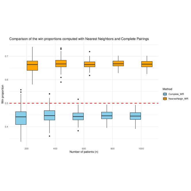
Figure 1: Comparison of the win proportion $p_{\mathrm{W}}$ computed with complete pairings and Nearest Neighbor pairings. Setting of Example˜1. Boxplots over 100 runs. The two approaches lead to different treatment recommendations (above and below 0.5).

Our first contribution in this paper is to expose the fact that considering different pairings between treated and controlled patients (complete pairings or Nearest Neighbor pairings) may lead to different treatment recommendations. We illustrate this in Figure˜1 on a simple synthetic example. This has major consequences: choosing different methodologies leads to different treatment recommendations. We argue that this is because these methods are typically limited to descriptive settings, relying on empirical procedures without a formal causal foundation. For instance, there is no well-defined estimand for what the Win Proportion, Win Ratio, and Net Benefit estimators seek at estimating. Despite their utility, integrating these methods into a cohesive causal inference framework remains underexplored. This paper formalizes Win Ratio and General Pairwise Comparisons approaches within a counterfactual paradigm (Splawa-Neyman et al., 1990), enabling a more robust interpretation of treatment effects in terms of potential outcomes. By doing so, we aim at addressing the limitations of existing methodologies to bridge the gap between descriptive statistical techniques and causal reasoning, facilitating their application in complex clinical trials and broadening their use to observational studies.

In particular, studying hierarchical comparisons in a causal inference frameworks leads to introducing estimands for our estimators. We show that depending on the choice of pairings considered, the estimand approached may change and have dramatically different properties, thus explaining Figure˜1. With complete pairings and in randomized controlled trials, the Win Proportion is a consistent estimator of the following causal estimand:

$$\mathbb{P}\left(Y_{i}\succ Y_{j}\right)\,,$$

where $i$ and $j$ are respectively two treated and controlled patients. This estimand is a population-level estimand. It as such does not capture the individual-level treatment effects: it is the probability that an individual sampled uniformly with treatment fares better than another individual sampled uniformly without treatment. An individual-level estimand would instead be the probability that a given individual fares better with than without treatment. Given $Y_{i}(1)$ and $Y_{i}(0)$ the potential outcomes of a given patient with and without treatment (Splawa-Neyman et al., 1990), this ideal individual-level estimand formally writes as:

$$\mathbb{P}\left(Y_{i}(1)\succ Y_{i}(0)\right)\,.$$

However, this causal estimand is non-identifiable. It depends on the joint distribution of the potential outcomes, which is never observed. These two estimands were previously mentionned in a series of works (Mao, 2017; Guo and Ni, 2022; Chen et al., 2024; Yin et al., 2022; Zhang et al., 2022; Chiaruttini et al., 2024).

Our next contribution is thus to introduce a new identifiable and individual-level estimand, that will serve as proxy for the non-identifiable individual-level causal estimand previously defined. Our proxy is a better proxy than the population-level estimand, as it compares the outcome of an individual being treated, with the outcome of a controlled patient that has the exact same features, rather than any random controlled patient. Informally, our newly introduced estimand writes as

$$\mathbb{P}\left(Y_{i}\succ Y_{i^{\prime}}\right)\,,$$

where $i$ is a treated patient, and $i^{\prime}$ an independent controlled patient that satisfies $X_{i^{\prime}}=X_{i}$ ($i^{\prime}$ may not exist, it is the result of a mind experiment). We show that in randomized controlled trials, the Win Proportion with Nearest Neighbors pairings is a consistent estimator for the causal estimand we introduce, thereby proving its identifiability. Using a simple example, we show that our newly introduced estimand should be preferred over the population-level estimand, making appear a paradox where changing the causal measure changes treatment effects. We provide discussions on the properties of our estimand in Section˜2.3.

Finally, the last part of the paper is devoted to estimating the estimand we introduce. In Section˜4, we extend the Nearest Neighbors approach to the observational setting by incorporating propensity weights. In order to face the fact that Nearest Neighbors may be slow to converge in the presence of high dimensional input features and to face their lack of robustness in the presence of missing data in the covariates, we introduce a distributional regression approach in Section˜4.2 to estimate our new causal estimand. The distributional regression estimators we propose benefit from very simple implementations, and as such we believe they can be easily used by practitioners. We finally propose a doubly-robust estimator, that combines the strengths of the distributional regression approach and of the weighted Nearest Neighbors approach.

1.2 Related works

Hierarchical Outcome Analysis and practical advancements.

Pocock et al. (2011); Buyse (2010) introduced the Win Ratio and Generalized Pairwise Comparisons with the Net Benefit of a treatment. These methodologies are inspired by Wilcoxon-Mann-Whitney tests (Wilcoxon, 1945; Mann and Whitney, 1947), that consist in testing if a real-valued random variable $Y$ is stochastically larger than another random variable $Z$. The quantity that arises in such tests is $\mathds{1}_{{\left\{Y\geqslant Z\right\}}}$ and its mean, $\mathbb{P}\left(Y\geqslant Z\right)$. Several studies have employed the Win Ratio or Generalized Pairwise Comparisons methodologies to analyze hierarchical outcomes. For instance, Pocock et al. (2023) used a stratified Win Ratio approach in the EMPULSE trial, which included 530 patients evenly split between treatment and placebo groups. Their analysis demonstrated how comparisons of all patient pairs contributed to "wins" for empagliflozin and placebo across four levels of the outcome hierarchy, resulting in an unstratified Win Ratio of 1.38, with accompanying confidence intervals and related metrics. They also discussed appropriate and inappropriate interpretations of this ratio. Similarly, Backer et al. (2024) applied hierarchical analysis to study reductions in treatment dosage and intensity for acute promyelocytic leukemia using Generalized Pairwise Comparisons, prioritizing efficacy outcomes such as event-free survival at two years over tolerability outcomes, including four pre-specified toxicities common in this context. In another example, Boentert et al. (2024) applied the Win Ratio methodology to the COMET trial (Diaz-Manera et al., 2021), a Phase 3 study on late-onset Pompe disease. Their analysis showcased how the Win Ratio approach could be used to assess multiple endpoints in the orphan drug context, providing a more comprehensive evaluation of treatment benefits compared to previous analyses of the COMET trial.

Redfors et al. (2020) provide a comprehensive overview of the Win Ratio methodology, offering insights into its design and reporting for clinical studies. Ajufo et al. (2023) highlight several fallacies associated with the Win Ratio and Generalized Pairwise Comparisons. These include the observation that a "win" does not always equate to a clinically meaningful benefit, emphasizing the importance of accounting for "ties" or "nulls" rather than ignoring them. They also caution that using patient-reported outcomes in comparisons may introduce biases and that baseline risk stratification may not fully balance the risk profiles of paired subjects. Additionally, Mao (2024) identify further limitations of hierarchical comparison methods, such as challenges related to outcome censoring. A major issue with current Win Ratio and Generalized Pairwise Comparisons lies in the fact that these methodologies are only restricted to Randomized Controlled Trials (RCTs) and cannot be applied to observational studies, and another unaddressed limit is missing data in covariates. Finally, Dong et al. (2018) proposed a stratified Win Ratio approach, inspired by stratified odds ratio approaches (Cochran, 1954; Mantel and Haenszel, 1959). Our approach and results in this paper tend towards recommending the use of as much stratification as possible when dealing with Win Ratio and more generally comparison-based estimators.

Formalization of hierarchical outcome analyses.

All previous cited works above provide guidances and recommendations based on empirical observations and trial examples. There has been advances towards formalizing estimands for hierarchical comparisons and adapting these methods to observational data, based on Wilcoxon-Mann-Whitney testing (Wilcoxon, 1945; Mann and Whitney, 1947). Mao (2017) formalized pairwise comparisons in a $U-$statistics setting, and provide (augmented) inverse propensity weighting for estimating a population-level estimand in observational studies. The estimand Mao (2017) introduced writes as the probability that a given randomly selected treated individual fares better than (i.e. wins against) another randomly selected controled individual, and is also studied by Chen et al. (2024); Yin et al. (2022) for rank-sum-tests or more generally for learning with contrast functions (Guo and Ni, 2022). This is a population-level estimand in the sense that it compares the distribution of the outcome of two randomly selected patient. Several subsequent works then drew inspiration from Mao (2017) to apply this in cancer studies (Chiaruttini et al., 2024) or refine the proposed method in the presence of dependent subjects (Zhang et al., 2022) or clusters (Zhang and Jeong, 2021).

Causal effect measures to assess treatment effects.

One of the key contribution of our paper is to design an adequate estimand for pairwise comparisons, that Win Ratio and Generalized Pairwise Comparisons methologies seek at approaching. The causal estimand we define is derived from a new causal measure. A causal measure is a functional of the joint distribution of the potential outcomes, and can vary from the Average Treatment Effect (ATE) with the Risk Difference (RD) to the Risk Ratio, the Odds Ratio, etc. Reporting results using different causal measures may lead to different conclusions or interpretations, and choosing the right is never straightforward (Colnet et al., 2024). Previous estimands related to the Win Ratio consist of an individual-level estimand that cannot be estimated due to non-identifiability issues, and of a population-level estimand that is identifiable, but that compares the distribution of the treated population, with the distribution of the control population (Mao, 2017; Guo and Ni, 2022). See Fay and Li (2024) for an extended discussion on individual and population-level estimands and causal measures, and Gao et al. (2024) for approaches to handle non-identifiable causal estimands. The estimand we introduce lies in-between the two previously cited estimands: it is individual-level and identifiable. As opposed to some causal measures like the risk-ratio that are not directly collapsible (Fay and Li, 2024; Groenwold et al., 2011; Didelez and Stensrud, 2021) where taking the population-level estimand ($\mathbb{E}\left[Y_{i}(1)\right]/\mathbb{E}\left[Y_{i}(0)\right]$ instead of $\mathbb{E}\left[Y_{i}(1)/Y_{i}(0)\right]$ for the risk ratio) makes sense and can be interpreted in terms of treatment recommendations ($\mathbb{E}\left[Y_{i}(1)\right]/\mathbb{E}\left[Y_{i}(0)\right]=2$ means that treating everyone leads to an averaged outcome twice larger compared to treating no one), in comparison-based estimands this is not the case, as will be highlighted in our paper. As such, one must be very careful at what one is estimating, and defining the true quantity of interest becomes even more important.

Finally, another example of application of our framework beyond hierarchical outcomes analysis is causal inference on distribution functions (Lin et al., 2023). If outcomes are general objects in a metric space (for instance, histograms), a contrast function $w(y,y^{\prime})=d(y,y^{\prime})$ can be used. The metric can for instance be the Wasserstein metric if we work with continuous histogram), quantifying how much two outcomes $y$ and $y^{\prime}$ are different. Here, the intuitive population-level causal measure would be to compute $\bar{y}_{1},\bar{y}_{0}$ the Wasserstein barycenters of outcomes in respectively treated and control groups. Our framework enables to go beyond such population-level estimands, while keeping identification possible.

2 Causal inference framework for Win Ratio and generalized pairwise comparisons

2.1 Definitions and assumptions

We classically assume that we have access to $n$ independent and identically distributed (i.i.d.) patients. Each patient $i\in[n]$ is characterized by his features vector $X_{i}$, that lies in some feature space $\mathcal{X}$, a treatment assignment $T_{i}\in{{\left\{0,1\right\}}}$, and an observed response (or outcome) $Y_{i}\in\mathcal{Y}$. $\mathcal{Y}$ is the outcome set, and outcomes might be multivariate (for instance, $\mathcal{Y}\subset\mathbb{R}^{d}$ with $d\geqslant 2$). $T_{i}=0$ and $T_{i}=1$ respectively correspond to patient $i$ being in the control group (non-treated) or in the test group (treated). Equivalently, the control and test groups can be replaced by two different treatment options. We use the potential outcome framework (Splawa-Neyman et al., 1990), that formalizes the concept of an intervention by positing the existence of two values $Y_{i}(0)$ and $Y_{i}(1)$ for the outcomes of interest, for the two situations where the patient has been exposed to treatment or not. These values are called potential outcomes, and they lie in some outcomes space $\mathcal{Y}$. The following assumption, often stated as the Stable Unit Treatment Values Assumption, is made throughout the paper, and states that the outcome is equal to the potential outcome given treatment.

Assumption 1 (SUTVA).

We have $Y_{i}=Y_{i}(T_{i})$ for all $i\in{{\left\{1,\ldots,n\right\}}}$.

We will also make the two following assumptions, often referred to as unconfoundedness and overlap/positivity, respectively. Both these assumptions will be directly verified in the randomized controlled trial setting (RCT setting, for which $T_{i}\perp\!\!\!\perp X_{i}$) that we will first consider in Section˜3. The observational setting considered after in Sections˜4 and 4.2 will rely on Assumptions˜2 and 3.

Assumption 2 (Unconfoundedness).

We have ${{\left\{Y_{i}(0),Y_{i}(1)\right\}}}\perp\!\!\!\perp T_{i}|X_{i}$.

Assumption 3 (Positivity).

There exists $\eta\in(0,1)$ such that for all $x\in\mathcal{X}$, we have

$$\eta\leqslant\pi(x)\leqslant 1-\eta\,,$$

where $\pi(x)=\mathbb{P}\left(T_{i}=1|X_{i}=x\right)$ is the probability of being treated given $X_{i}=x$.

We want to know if a given patient would fare better under treatment than without it. In the potential outcomes framework, there exists several causal measures to quantify this, amongst which the Risk Difference (RD) if $\mathcal{Y}\subset\mathbb{R}$, for which the Average Treatment Effect writes as:

$$\tau_{\mathrm{RD}}\stackrel{{\scriptstyle\text{def}}}{{=}}\mathbb{E}\left[Y_{i}(1)-Y_{i}(0)\right]\,.$$

However, we would like to handle more general outcomes, and Section˜2.3 defines more general causal measures.

We introduce the “win” function on $\mathcal{Y}\times\mathcal{Y}$, that quantifies how a given outcome $y\in\mathcal{Y}$ fares when compared to another outcome $y^{\prime}\in\mathcal{Y}$. Our framework generalizes the lexicographic order beyond the setting introduced by Pocock et al. (2011).

Definition 1 (Win function).

Let

$$w\,:\,(y,y^{\prime})\in\mathcal{Y}^{2}\mapsto w(y,y^{\prime})\in[0,1]\,,$$

be the win function, taking two outputs $y,y^{\prime}$ to compare, and outputing a value between 0 and 1.

A typical example is:

$$w(y|y^{\prime})=\left\{\begin{aligned} &1\quad&\text{if}&\qquad y\succ y^{\prime}\\ &\frac{1}{2}\quad&\text{if}&\qquad y\sim y^{\prime}\\ &0\quad&\text{if}&\qquad y\prec y^{\prime}\end{aligned}\right.\qquad,$$ (1)

where $\succ$ is an order on $\mathcal{Y}$, that we refer to as clinical order, and $\sim$ means that the outcomes are similar or cannot be compared. If “ties” are discarded, the win function writes as:

$$w(y|y^{\prime})=\left\{\begin{aligned} &1\quad&\text{if}&\qquad y\succ y^{\prime}\\ &0\quad&\text{if}&\qquad y\preceq y^{\prime}\end{aligned}\right.\qquad,$$ (2)

Pocock et al. (2011) first introduced the Win Ratio to handle composite endpoints in clinical trials based on clinical priorities, without formalizing it using the potential outcomes framework. In their example, outcomes $Y_{i}$ are of dimension $2$ and potential outcomes $Y_{1}(t),Y_{2}(t)\in\mathbb{R}\cup{{\left\{\infty\right\}}}$ would respectively correspond to the time after treatment (or non treatment) before an eventual cardiovascular death event, and the time after (non-)treatment before an eventual heart-failure hospitalization. $Y_{i}(t)=\infty$ means that no such event occurred. The win function here writes as: $w(y|y^{\prime})=\mathds{1}_{{\left\{y_{1}>y_{1}^{\prime}\right\}}}+\mathds{1}_{{\left\{y_{1}=y_{1}^{\prime}\,,\,y_{2}>y_{2}^{\prime}\right\}}}$, i.e. $w(y|y^{\prime})=1$ if and only if $y$ is strictly larger than $y^{\prime}$ for the lexicographic order. Note that in this example, ties are counted as losses, which may not always be the case, as this may cause problems when ties should not be discarded nor treated as losses, as pointed out by Ajufo et al. (2023).

Notations and terminology.

For a sequence $(Z_{n})_{n\geqslant 0}$ of random variables with values in a metric space $(\mathcal{Z},d)$ and $Z$ a random variable in $\mathcal{Z}$, we say that $Z_{n}$ converges in probability towards $Z$ if for any $\varepsilon>0$ we have that $\mathbb{P}\left(d(Z_{n},Z)>\varepsilon\right)\to 0$. We say that a measurable event $\mathcal{E}$ is almost sure if its probability is 1. We say that $Z_{n}$ converges almost surely towards some value $\ell$ if the event ${{\left\{Z_{n}\to\ell\right\}}}$ is almost sure. $Z_{n}$ is a consistent estimator of some quantity $\ell$ if $Z_{n}$ converges in probability towards the constant random variable $\ell$.

2.2 Traditional Win Ratio, Net-Benefit and Mann-Whitney-Wilcoxon comparison estimators

Let $\mathcal{N}_{t}={{\left\{i:T_{i}=t\right\}}}$ for $t=0,1$ be respectively the control and treated groups. Below, we formalize the estimators used by Pocock et al. (2011); Buyse (2010) for Win Ratio and Generalized Comparisons. We refer to these estimators as traditional or historical Win Ratio and Net-Benefit. Pocock et al. (2011); Buyse (2010) form pairs $\mathcal{C}\subset\mathcal{N}_{1}\times\mathcal{N}_{0}$ and define

$$n_{\mathrm{W}}\stackrel{{\scriptstyle\text{def}}}{{=}}\sum_{(y,y^{\prime})\in\mathcal{C}}w(y|y^{\prime})\,,$$ (3)

as the number of wins and $n_{\mathrm{L}}=|\mathcal{C}|-n_{\mathrm{W}}$ as the number of losses. The Win Proportion is defined as:

$$\hat{p}_{\mathrm{W}}\stackrel{{\scriptstyle\text{def}}}{{=}}\frac{n_{\mathrm{W}}}{n_{\mathrm{W}}+n_{\mathrm{L}}}\,,$$ (4)

and the Win Ratio (Pocock et al., 2011) is then defined as:

$$\hat{R}_{\mathrm{WR}}\stackrel{{\scriptstyle\text{def}}}{{=}}\frac{\hat{p}_{\mathrm{W}}}{1-\hat{p}_{\mathrm{W}}}=\frac{n_{\mathrm{W}}}{n_{\mathrm{L}}}\,.$$ (5)

Another related quantity is the Net Benefit (Buyse, 2010):

$$\hat{\Delta}_{\mathrm{NB}}\stackrel{{\scriptstyle\text{def}}}{{=}}2\hat{p}_{\mathrm{W}}-1=\frac{n_{\mathrm{W}}-n_{\mathrm{L}}}{n_{\mathrm{W}}+n_{\mathrm{L}}}\,.$$ (6)

Computing $\hat{p}_{\mathrm{W}}$ leads to values for both $\hat{R}_{\mathrm{WR}}$ and $\hat{\Delta}_{\mathrm{NB}}$. Based on $\hat{R}_{\mathrm{WR}}$, $\hat{\Delta}_{\mathrm{NB}}$ or $\hat{p}_{\mathrm{W}}$, the treatment $T=1$ can be judged favorable compared to non-treatment (or equivalently, to the treatment option corresponding to $T=0$) if

$$\hat{p}_{\mathrm{W}}>\frac{1}{2}\,,$$

which is equivalent to $\hat{R}_{\mathrm{WR}}>1$ or $\hat{\Delta}_{\mathrm{NB}}>0$. Uncertainties and variance needs however to be taken into account to rule out a treatment option for another.

The choice of the set of pairs $\mathcal{C}\subset\mathcal{N}_{0}\times\mathcal{N}_{1}$ of control and test individuals used to compute the number of wins in Equation˜3 has a crucial impact on the quantity being computed. The pair set $\mathcal{C}$ might vary from the two natural following extremes:

1. Complete pairings, for which we have:

   $$\mathcal{C}_{\mathrm{Tot}}\stackrel{{\scriptstyle\text{def}}}{{=}}\mathcal{N}_{0}\times\mathcal{N}_{1}\,.$$

   Complete pairings are the prevalent strategy in Win Ratio or Generalized Pairwise Comparisons analyses.

2. Nearest-neighor pairings, for which

   $$\mathcal{C}_{\mathrm{NN}}\stackrel{{\scriptstyle\text{def}}}{{=}}{{\left\{(i,\sigma^{\star}(i))\,|\,i\in\mathcal{N}_{0}\right\}}}\,,$$

   where $\sigma^{\star}(i):\mathcal{N}_{0}\to\mathcal{N}_{1}$ matches $i\in\mathcal{N}_{0}$ to the treated individual $j\in\mathcal{N}_{1}$ that has closest features in $\mathcal{X}$ i.e., $\sigma^{\star}(i)\in\operatorname{argmin}_{j\in\mathcal{N}_{1}}{{\left\|X_{i}-X_{j}\right\|}}^{2}$. $\mathcal{C}_{\mathrm{NN}}$ can also be generalized to $k-$Nearest Neighbors. For continuous features, Nearest Neighbors can be naturally applied after an eventual reweighting of the different features, to prevent from scale effects. For categorical features, Nearest Neighbors can be applied with one-hot encodings for instance, leading to Hamming-distances. In the presence of different categorical features of different importance, these can be weighted according to their importance.

As highlighted in Example˜1, using different pairings leads to different Win Proportions (and thus to different Win Ratios and Net Benefits), to the point where treatment recommendations may even differ.

Example 1.

Suppose that we have $n=6$ individuals with univariate and real outcomes ($\mathcal{Y}\subset\mathbb{R}$). Assume that for $i=1,2,3,4$, individuals are men (for which $X_{i}=0$) and we have $Y_{i}(1)=y_{1}>y_{0}=Y_{i}(0)$ while for $i=5,6$ individuals are women (for which $X_{i}=1$) and we have $Y_{i}(1)=y_{1}<y_{0}=Y_{i}(0)$, and that for $i\in{{\left\{1,\ldots,6\right\}}}$ we have $T_{i}=1$ if $i$ is an odd number. Assume then that $y_{0}^{\prime}>y_{1}>y_{0}>y_{1}^{\prime}$. Then, we have:

$$\hat{p}_{\mathrm{W}}=\left\{\begin{aligned} &\frac{2}{3}&\quad&\text{if}&\quad&\mathcal{C}=\mathcal{C}_{\mathrm{NN}}\\ &\frac{4}{9}&\quad&\text{if}&\quad&\mathcal{C}=\mathcal{C}_{\mathrm{Tot}}\\ \end{aligned}\right.\quad,$$

leading to $\hat{p}_{\mathrm{W}}>1/2$ or $\hat{p}_{\mathrm{W}}<1/2$ and thus to different treatment decisions depending on the coupling pairs chosen. Here, treatment favors $4$ out of the $6$ patients, while no-treatment only favors $2$ out of the $6$: complete pairings thus favors the treatment option that benefits to only a minority of patients. This is further illustrated in Figure˜1 in the setting of Example˜1, with $n/3$ women and $2n/3$ men, in a RCT setting with treatment probability of $1/2$.

2.3 From estimators to causal measures and estimands

The quantities introduced so far — $\hat{p}_{\mathrm{W}},\hat{R}_{\mathrm{WR}},\hat{\Delta}_{\mathrm{NB}}$ —, are data-dependent estimators (hence the $\hat{\cdot}$ notation). To efficiently capture treatment effects and treatment comparisons, we need to first answer the following crucial question: what is the estimand that these estimators seek at estimating ? In this subsection, we review the two causal estimands previously defined and studied for generalized comparisons and Win Ratio analyses, before introducing our new estimand. The first estimand is a natural individual-level estimand, but cannot be estimated as it is not identifiable. Most works therefore introduced a population-level estimand, as a proxy for the non-identifiable individual-level causal estimand. This causal estimand may however not capture treatment effects correctly, hence our new causal estimand that is both individual-level and identifiable.

A natural but non-identifiable causal estimand.

In our causal inference framework, we wish to determine if individuals would fare better if treated or non-treated. Here, $w$ is a contrast function that compares two outcomes $y,y^{\prime}\in\mathcal{Y}$: $w(y|y^{\prime})$ quantifies the relative favorability of $y$ compared to $y^{\prime}$. If we worked with the Risk Difference, we would have $w(y|y^{\prime})=y-y^{\prime}$, and the ATE would write $\tau_{\mathrm{ATE}}=\mathbb{E}\left[w(Y_{i}(1)|Y_{i}(0))\right]=\mathbb{E}\left[Y_{i}(1)-Y_{i}(0)\right]$. In the general case, with general contrast functions (our “win” function), this leads to consider the following quantity:

$$\tau_{\mathrm{indiv}}\stackrel{{\scriptstyle\text{def}}}{{=}}\mathbb{E}\left[w(Y_{i}(1)|Y_{i}(0))\right]\,.$$ (7)

The quantity $\tau_{\mathrm{indiv}}$ is a causal effect measure (or causal measure, for short) and a causal estimand, that compares the two potential outcomes of a given individual using the contrats/win function $w$. If $w$ is as in Equation˜1, we have:

$$\tau_{\mathrm{indiv}}=\mathbb{P}\left(Y_{i}(1)\succ Y_{i}(0)\right)+\frac{1}{2}\mathbb{P}\left(Y_{i}(1)\sim Y_{i}(0)\right)\,,$$

while if $w$ is as in Equation˜2, we have:

$$\tau_{\mathrm{indiv}}=\mathbb{P}\left(Y_{i}(1)\succ Y_{i}(0)\right)\,.$$

However, as highlighted by several works (Mao, 2017; Guo and Ni, 2022; Chen et al., 2024; Yin et al., 2022; Zhang et al., 2022; Chiaruttini et al., 2024), this causal measure is non-identifiable since estimating it in general requires the knowledge of the joint distribution of the potential outcomes, which is never observed . $\tau_{\mathrm{indiv}}$ is indeed an individual-level causal estimand (Fay and Li, 2024), as it is directly a function of the joint probability distribution $\mathcal{P}({{\left\{Y_{i}(0),Y_{i}(1)\right\}}})$, as opposed to population-level causal estimands that are functions of ${{\left\{\mathcal{P}(Y_{i}(0)),\mathcal{P}(Y_{i}(1))\right\}}}$. What makes it possible to estimate $\mathbb{E}\left[w(Y_{i}(1)|Y_{i}(0))\right]$ with the Risk Difference is the fact that thanks to the linearity of the contrast function $w$, $\mathbb{E}\left[w(Y_{i}(1)|Y_{i}(0))\right]$ is both a population and an individual-level causal measure.

A population-level causal estimand.

To circumvent this non-identifiability issue of individual-level causal measures, Mao (2017); Guo and Ni (2022); Chen et al. (2024); Yin et al. (2022); Zhang et al. (2022); Chiaruttini et al. (2024) consider a population-level causal measure $\tau_{\mathrm{pop}}$ instead of the indivual-level one that defines $\tau_{\mathrm{indiv}}$. Their causal measure writes as:

$$\tau_{\mathrm{pop}}\stackrel{{\scriptstyle\text{def}}}{{=}}\mathbb{E}\left[w(Y_{i}(1)|Y_{j}(0))\right]\,,$$ (8)

where $i$ and $j$ are two different and independent individuals. Considering two independent individuals leads to a different measure, that can now be estimated. We will show in Theorem˜1 that with total pairings, $\hat{p}_{\mathrm{W}}$ in Equation˜9 is a consistent estimator of $\tau_{\mathrm{pop}}$.

Our individual-level and identifiable causal estimand.

Using $\tau_{\mathrm{pop}}$ leads to comparing individuals that may not be comparable, hence the following causal measure we introduce. It is an identifiable relaxation of $\tau_{\mathrm{indiv}}$, defined by comparing patient $i$ with features $X_{i}$ to an independent copy that has the same features. $\tau_{\star}$ is an individual-level causal estimand.

Definition 2.

For $x\in\mathcal{X}$, let ${{\left\{Y^{(x)}(0),Y^{(x)}(1)\right\}}}$ be an independent copy of ${{\left\{Y_{i}(0),Y_{i}(1)\right\}}}|X_{i}=x$. Let

$$\tau_{\star}(x)\stackrel{{\scriptstyle\text{def}}}{{=}}\mathbb{E}\left[w(Y^{(x)}(1)|Y_{i}(0))|X_{i}=x\right]\,,$$

and define

$$\tau_{\star}\stackrel{{\scriptstyle\text{def}}}{{=}}\mathbb{E}\left[w(Y^{(X_{i})}(1)|Y_{i}(0))\right]\,.$$ (9)

The quantities defined $\tau_{\star}(x)$ and $\tau_{\star}$ are respectively a conditional effect measure and a causal effect measure (Pearl, 2009). By construction, the causal measure built satisfies direct collapsibility (Colnet et al., 2024, Definition 4) and is logic-respecting (Colnet et al., 2024, Definition 6). We will show in Theorem˜1 that the causal estimand $\tau_{\star}$ is identifiable as opposed to $\tau_{\mathrm{indiv}}$, since for $\mathcal{C}=\mathcal{C}_{\mathrm{NN}}$ the estimator $\hat{p}_{\mathrm{W}}$ (Equation˜4) is consistent for $\tau_{\star}$.

Remark 1.

Under additional assumptions such as potential independence (i.e., $Y_{i}(1)\perp\!\!\!\perp Y_{i}(0)\,|\,X_{i}$), we have that $\tau_{\star}=\tau_{\mathrm{indiv}}$. This assumption of potential independence is however quite strong and may be considered unlikely to hold true. It means that all that accounts for treatment effects is included in $X_{i}$, precluding e.g. any unmeasured factor. Some examples (such as for instance comparing 2 different doses of a same treatment) make it impossible to assume conditional independence in general, hence the appeal of $\tau_{\star}$, since Definition˜2 does not need to make any assumption for $\tau_{\star}$ to be well-defined.

We now define the statistical estimands related to our causal measures and to our causal estimands. Recall that statistical estimands are functions of measurable quantities; as such, they cannot make appear counterfactual quantities such as potential outcomes, which is not the case for causal measures and causal estimands. For instance, the statistical estimand related to the causal estimand $\tau_{\mathrm{RD}}$ is $\mathbb{E}\left[Y_{i}|T_{i}=1\right]-\mathbb{E}\left[Y_{i}|T_{i}=1\right]$. For the population-level causal measure $\tau_{\mathrm{pop}}$, the related statistical estimand writes as:

$$\mathbb{E}\left[w(Y_{i}|Y_{j})|T_{i}=1,T_{j}=0\right]\,,$$

while the statistical estimand related to $\tau_{\star}$ writes as

$$\mathbb{E}\left[w(Y^{(X_{i})}(1),Y_{i})|T_{i}=0\right]\,,$$

or, equivalently:

$$\mathbb{E}\left[w(Y_{i},Y^{(X_{i})}(0))|T_{i}=1\right]\,.$$

Under Assumption˜1 (SUTVA), we have that these statistical estimands are equal to their associated causal estimands.

From the estimands $\tau=\tau_{\star}$ or $\tau=\tau_{\mathrm{pop}}$, the Win Ratio estimand related to the estimator $\hat{R}_{\mathrm{WR}}$ defined in Equation˜5 writes as:

$$R_{\mathrm{WR}}\stackrel{{\scriptstyle\text{def}}}{{=}}\frac{\tau}{1-\tau}\,,$$

while the Net Benefit estimand related to the estimator $\hat{\Delta}_{\mathrm{NB}}$ defined in Equation˜6 writes as:

$$\Delta_{\mathrm{NB}}\stackrel{{\scriptstyle\text{def}}}{{=}}2\tau-1\,.$$

Remark 2.

Having estimators and confidence intervals for estimating $\tau$ with some estimator $\hat{\tau}$ is equivalent to having estimates and confidence intervals for $R_{\mathrm{WR}}$ or $N_{\mathrm{NB}}$ for estimators $\hat{\Delta}=2\hat{\tau}-1$ and $\hat{R}=\frac{\hat{\tau}}{1-\hat{\tau}}$. Indeed, if we have a confidence interval of the form $\mathbb{P}\left(\hat{\tau}\in[\tau-\varepsilon_{1},\tau+\varepsilon_{2}]\right)\geqslant 1-\alpha$, we also have $\mathbb{P}\left(\hat{\Delta}\in[\Delta_{\mathrm{NB}}-2\varepsilon_{1},\Delta_{\mathrm{NB}}+2\varepsilon_{2}]\right)\geqslant 1-\alpha$ and $\mathbb{P}\left(\hat{R}\in[R_{\mathrm{WR}}-\varepsilon_{1}^{\prime},R_{\mathrm{WR}}-\varepsilon_{2}^{\prime}]\right)\geqslant 1-\alpha$, where $\varepsilon_{1}^{\prime}=\frac{\tau}{1-\tau}-\frac{\tau-\varepsilon_{1}}{1+\varepsilon_{1}-\tau}$ and $\varepsilon_{2}=\frac{\tau+\varepsilon_{2}}{1-\varepsilon_{2}-\tau}-\frac{\tau}{1-\tau}$ if $0<\tau-\varepsilon_{1}$ and $\tau+\varepsilon_{2}<1$.

Remark 3 (On the well-posedness of Definition˜2).

Let $(E,\mathcal{E})$ and $(F,\mathcal{F})$ be two probability spaces. $\nu:E\times\mathcal{F}\to[0,1]$ is a transition kernel if it satisfies $\forall x\in E\,,\,\nu(x,\cdot)$ is a probability measure on $(F,\mathcal{F})$ and $\forall B\in\mathcal{F}\,,\,\nu(\cdot,B)$ is $\mathcal{E}-$measurable. If $X\in\mathbb{R}^{p}$ and $Y\in\mathbb{R}^{d}$, the conditinal law of $Y$ given $X$ is a kernel $\nu$ on $(\mathbb{R}^{d}\times\mathcal{B}(\mathbb{R}^{p}))$ that satisfies:

$$\mathbb{P}_{(X,Y)}=\mathbb{P}_{X\cdot\nu}\,,\quad\text{i.e.}\quad\forall(A,B)\in\mathcal{B}(\mathbb{R}^{p})\times\mathcal{B}(\mathbb{R}^{d})\,,\quad\mathbb{P}\left(X\in A,Y\in B\right)=\int_{x\in A}\nu(x,B)\mathbb{P}_{X}({\rm d}x)\,.$$

Such a transition kernel always exists: this is Miloslav Jiřina’s Theorem (Jiřina, 1959) for Borelian measures and random variables. We write

$$\mathbb{P}\left(Y\in B|X=x\right)\stackrel{{\scriptstyle\text{def}}}{{=}}\nu(x,B)\,.$$

To build two independent copies of $Y$ given $X=x$, we thus draw $Y_{x},Y^{\prime}_{x}$ with:

$$\forall(B,B^{\prime})\in\mathcal{B}(\mathbb{R}^{d})^{2}\,,\quad\mathbb{P}\left(Y_{x}\in B\,,\,Y_{x}^{\prime}\in B^{\prime}\right)=\nu(x,B)\nu(x,B^{\prime})\,.$$

We thus have created a copy of $Y$ that satisfies the two following properties: (i) it is independent of $Y$ conditionally on $X$; (ii) conditionally on $X$, the distributions of $Y^{\prime}$ and $Y$ are the same. Their joint distribution with $X$ writes as:

$$\mathbb{P}\left(X\in A\,,\,Y\in B\,,\,Y^{(X)}\in B^{\prime}\right)=\mathbb{P}\left(X\in A\right)\mathbb{E}\left[\nu(X,B)\nu(X,B^{\prime})|X\in A\right]\,,$$

for all $(A,B,B^{\prime})\in\mathcal{B}(\mathbb{R}^{p})\times\mathcal{B}(\mathbb{R}^{d})^{2}$.

Example˜2 below is the estimand-wise version of Example˜1. It shows that the causal measures $\tau_{\star}$ and $\tau_{\mathrm{pop}}$ are not equivalent and may lead to different treatment recommendations if populations are heterogeneous. In particular, Example˜2 justifies our preference and recommendations towards using $\tau_{\star}$ over $\tau_{\mathrm{pop}}$.

Example 2.

Assume that outcomes are univariate ($Y_{i}(0),Y_{i}(1)\in\mathbb{R}$), and that $\mathcal{X}=\mathcal{X}_{1}\cup\mathcal{X}_{2}$ with $\mathbb{P}\left(X_{i}\in\mathcal{X}_{1}\right)=1-\alpha$, $\mathbb{P}\left(X_{i}\in\mathcal{X}_{2}\right)=\alpha$ such that:

$$Y_{i}(1)=y_{1}>y_{0}=Y_{i}(0)|X_{i}\in\mathcal{X}_{1}\,,\quad Y_{i}(1)=y^{\prime}_{1}<y^{\prime}_{0}=Y_{i}(0)|X_{i}\in\mathcal{X}_{2}\,,$$

almost surely. We then have, if $y_{0}^{\prime}>y_{1}>y_{0}>y_{1}^{\prime}$:

$$\mathbb{E}\left[w(Y^{(X_{i})}(1)|Y_{i}(0))\right]=1-\alpha\,,\qquad\mathbb{E}\left[w(Y_{i}(1)|Y_{j}(0))\right]=(1-\alpha)^{2}\,.$$

Thus, if $\frac{1}{2}>\alpha>1-\frac{1}{\sqrt{2}}$, we have:

$$\mathbb{E}\left[w(Y^{(X_{i})}(1)|Y_{i}(0))\right]>\frac{1}{2}>\mathbb{E}\left[w(Y_{i}(1)|Y_{j}(0))\right]\,,$$

leading to different conclusions in terms of treatment efficacy (see Figure˜1).

We highlight the fact that the phenomenon appearing in Example˜2 is not reminiscent of Simpson’s paradox (Simpson, 1951; Wagner, 1982), as understood in the popular sense. Simpson’s paradox states a trend might appear in all subgroups of a population, but still reverse when considering the average over all population. Here, the paradox in Example˜2 is of a very different nature, since in both cases the average over the whole population is considered. The difference lies in the way the average is taken: different causal measures might lead to different treatment effects. Taking the average of individual effects over the global population (as done when considering $\tau_{\star}$) or comparing the whole treated group distribution with the control distribution (as done when considering $\tau_{\mathrm{pop}}$) can lead to opposite trends.

Similarly to $\tau_{\mathrm{pop}}$, $\tau_{\star}$ it serves as a computable proxy to approximate the ideal value $\tau_{\mathrm{indiv}}$ that cannot be approximated in general. We however argue that, thanks to simple examples such as the one just above, $\tau_{\star}$ is a better proxy than $\tau_{\mathrm{pop}}$, since it captures more information. This is intuitively the case: both $(Y^{(X_{i})}(1),Y_{i}(0))$ and $(Y_{j}(1),Y_{i}(0))$ are couplings of the random variables $Y_{i}(1)$ and $Y_{i}(0)$. The coupling $(Y^{(X_{i})}(1),Y_{i}(0))$ is however naturally closer to the coupling $(Y_{i}(1),Y_{i}(0))$ than the coupling $(Y_{j}(1),Y_{i}(0))$, since $(Y^{(X_{i})}(1),Y_{i}(0))$ takes into account covariate effects, leading to:

$$d_{\ell^{2}}\big{(}(Y^{(X_{i})}(1),Y_{i}(0))\,,\,(Y_{i}(1),Y_{i}(0))\big{)}\leqslant d_{\ell^{2}}\big{(}(Y_{j}(1),Y_{i}(0))\,,\,(Y_{i}(1),Y_{i}(0))\big{)}\,,$$

if the marginals are absolutely continuous with respect to the Lebesgue measure, and where $d_{\ell^{2}}$ is the $\ell^{2}$ distance between densities. Finally, next proposition formalizes the excess risk when using $\tau_{\star}$ or $\tau_{\mathrm{pop}}$ as proxis for $\tau_{\mathrm{indiv}}$.

Proposition 1.

We have:

$$\left|\tau_{\star}-\tau_{\mathrm{indiv}}\right|\leqslant d_{\mathrm{TV}}(P_{Y^{(X_{i})}(1),Y_{i}(0)},P_{Y_{i}(1),Y_{i}(0)})\,,$$

and

$$\left|\tau_{\mathrm{pop}}-\tau_{\mathrm{indiv}}\right|\leqslant d_{\mathrm{TV}}(P_{Y_{j}(1),Y_{i}(0)},P_{Y_{i}(1),Y_{i}(0)})\,,$$

where $P_{Y^{(X_{i})}(1),Y_{i}(0)},P_{Y_{i}(1),Y_{i}(0)},P_{Y_{j}(1),Y_{i}(0)}$ are respectively the joint distributions of $(Y^{(X_{i})}(1),Y_{i}(0))$, $(Y_{i}(1),Y_{i}(0))$ and $(Y_{i}(1),Y_{j}(0))$, and $d_{\mathrm{TV}}$ is the total-variation distance between distributions. Furthermore, if the win function $w$ is $1-$Lipschitz, we have that:

$$\left|\tau_{\star}-\tau_{\mathrm{indiv}}\right|\leqslant\mathcal{W}_{1}(P_{Y^{(X_{i})}(1),Y_{i}(0)},P_{Y_{i}(1),Y_{i}(0)})\,,$$

and

$$\left|\tau_{\mathrm{pop}}-\tau_{\mathrm{indiv}}\right|\leqslant\mathcal{W}_{1}(P_{Y_{j}(1),Y_{i}(0)},P_{Y_{i}(1),Y_{i}(0)})\,,$$

where $\mathcal{W}_{1}$ is the $1-$Wasserstein distance between distributions.

3 Consistency of traditional Win Ratio, Net-Benefit and Win Proportions in the RCT setting

In this section, we study $\hat{p}_{\mathrm{W}}$ in light of the causal measures we previously defined. The quantity $\hat{p}_{\mathrm{W}}$ is the Win Proportion (Equation˜4), that is used to compute $\hat{R}_{\mathrm{WR}}$ and $\hat{\Delta}_{\mathrm{NB}}$, referred to as traditional Win Ratio and Net-Benefit estimators. As expected from Examples˜1 and 2, the behavior of $\hat{p}_{\mathrm{W}}$ crucially depends on the pairings considered. The following theorem shows that, in a Randomized Controlled Trial (RCT) setting, the Win Proportion is the most natural estimator for the estimands $\tau=\tau_{\star}$ and $\tau=\tau_{\mathrm{pop}}$. Indeed, for a Nearest Neighbor pairing choice, the Win Proportion is a consistent estimator of $\tau_{\star}$, while for a complete pairing choice the Win Proportion is a consistent estimator of $\tau_{\mathrm{pop}}$.

Theorem 1 (Consistency of Win Ratio).

Let

$$\hat{p}_{W}^{(n_{0},n_{1},\mathcal{C})}\stackrel{{\scriptstyle\text{def}}}{{=}}\frac{1}{|\mathcal{C}|}\sum_{(i,j)\in\mathcal{C}}w(Y_{j}|Y_{i})\,,$$

for $\mathcal{C}\subset\mathcal{N}_{0}\times\mathcal{N}_{1}$. Assume that Assumptions˜1, 2 and 3 hold, and assume further that we are in the RCT setting: $T_{i}\perp\!\!\!\perp X_{i}$.

1. Complete pairing. We have:

   $$\hat{p}_{W}^{(n_{0},n_{1},\mathcal{C}_{\mathrm{Tot}})}\underset{\mathbb{P}}{\longrightarrow}\tau_{\mathrm{pop}}\stackrel{{\scriptstyle\text{def}}}{{=}}\mathbb{E}\left[w(Y_{i}(1)|Y_{j}(0))\right]\,,\quad i\neq j\,,$$

   where the limit in probability is taken as $n_{0},n_{1}\to\infty$ and $\mathcal{C}_{\mathrm{Tot}}=\mathcal{N}_{0}\times\mathcal{N}_{1}$.

2. Nearest Neighbor. Assume that $(x,y)\mapsto\mathbb{E}\left[w(Y_{i}(1)|y)|X_{i}=x\right]$ is continuous in its first variable $x$ and that $\mathcal{X}$ is compact. Then, let $\sigma^{\star}:\mathcal{N}_{0}\to\mathcal{N}_{1}$ be defined as:

   $$\forall i\in\mathcal{N}_{1}\,,\quad\sigma^{\star}(i)\in\operatorname{argmin}_{j\in\mathcal{N}_{1}}{{\left\|X_{i}-X_{j}\right\|}}\,,$$

   where if there are two possible choices or more for $\sigma^{\star}(i)$, we choose uniformly at random. Let $\mathcal{C}_{\mathrm{NN}}={{\left\{(i,\sigma^{\star}(i)),i\in\mathcal{N}_{0}\right\}}}$. We have:

   $$\hat{p}_{W}^{(n_{0},n_{1},\mathcal{C}_{\mathrm{NN}})}\underset{\mathbb{P}}{\longrightarrow}\tau_{\star}\stackrel{{\scriptstyle\text{def}}}{{=}}\mathbb{E}\left[\mathbb{E}\left[w(Y^{(X_{i})}(1)|Y_{i}(0))|X_{i}\right]\right]\,,$$

   where the limit in probability is taken as $n_{0},n_{1}\to\infty$.

The consistency results of Theorem˜1 formalize the intuition brought by Examples˜1 and 2 and illustrated in Figure˜1. The choice of pairing $\mathcal{C}$ is crucial, and leads to the estimation of very different quantities. For complete pairings $\mathcal{C}_{\mathrm{Tot}}$, the causal estimand that is estimated is the population-level one, $\tau_{\mathrm{pop}}$. For Nearest Neighbor pairings $\mathcal{C}_{\mathrm{NN}}$, the causal estimand that is estimated is the individual-level one that we introduced, $\tau_{\star}$, defined in Definition˜2. As highlighted in Examples˜1 and 2 and in Figure˜1, complete pairings and the population-level causal estimand have undesired behaviors and may even lead to different treatment recommendations. When the features $X_{i}$ are expressive enough, this fallacy of $\tau_{\mathrm{pop}}$ and of complete pairings is solved by considering our causal measure $\tau_{\star}$ and Nearest Neighbor pairings instead.

However, it is worth mentioning that, while $\tau_{\star}$ seems like the causal estimand one would seek at approaching, using Nearest Neighbor pairings to approach $\tau_{\star}$ has some downsides too. The first weakness of this approach is the fact that it is restricted to the RCT setting: the consistency result above in Theorem˜1.2 crucially relies on $T_{i}$ being independent of $X_{i}$. A first direction will thus be to relax the RCT setting to an observational one: this is what we do in Section˜4, where we combine an Inverse Propensity Weighting approach with Nearest Neighbor pairings. Then, the second weakness of this Nearest Neighbor approach is that it suffers from the curse of high dimensions: if the convergence speed in terms of samples $n$ required will drop exponentially as the dimension of the features $X_{i}$ increases. This is a known weakness of Nearest Neighbors approach in general (Biau and Devroye, 2015). Although they are one the most studied non-parametric learning methods for which theoretical results can be derived, Nearest Neighbors suffer from the fact that in high dimensions, points are likely to be separated if $n$ is not exponentially large in the dimension. This motivates our aim for a more general and systemic method to estimate our causal estimand $\tau_{\star}$: in Section˜4.2, we provide a distributional regression point of view on the problem and develop new methodologies for efficiently estimating $\tau_{\star}$. This new approach also has the benefit of being able to handle missing values in the covariates, unlike Nearest Neighbors approaches.

Finally, we conclude this section with Remark˜4: forming risk strata may be an interesting strategy, that lies in-between the two extreme choices $\mathcal{C}_{\mathrm{Tot}}$ and $\mathcal{C}_{\mathrm{NN}}$ for pairing sets. The causal estimand related to a strata function can also be defined, and we expect results similar to those of Theorem˜1 to hold. We argue that the individual-level causal estimand $\tau_{\star}$ can in fact be recovered using infinitesimal stratas, further justifying the strength of Definition˜2.

Remark 4 (Win Ratio and comparisons with strata).

The following notion of strata could be developed further, as an in-between the extreme cases presented in Theorem˜1. Let $r:\mathcal{X}\to\mathcal{R}$ be a risk strata function, on some metric space $(\mathcal{R},d)$. Patients with similar risks ($d(r(X_{i}),r(X_{j}))$ small) are expected to have similar control and treated behaviors. Using this strata, several studies build the following pairs of treated and control patients:

$$\mathcal{C}_{\hat{r},\varepsilon}\stackrel{{\scriptstyle\text{def}}}{{=}}{{\left\{(i,j)\in\mathcal{N}_{0}\times\mathcal{N}_{1}\,|\,d(r(X_{i}),r(X_{j}))\leqslant\varepsilon\right\}}}\,,$$

to obtain the estimator $\hat{p}_{\mathrm{W}}$ (Equation˜4) using these pairs. Now, define the $\varepsilon-$strata causal estimand as:

$$\tau_{\star}^{r,\varepsilon}\stackrel{{\scriptstyle\text{def}}}{{=}}\mathbb{P}\left(Y_{i}(1)\succ Y_{j}(0)|d(r(X_{i}),r(X_{j}))\leqslant\varepsilon\right)\,,$$

where $i$ and $j$ are two different and independent indices. Under adequate, if $\mathcal{C}=\mathcal{C}_{\hat{r},\varepsilon}$ we expect to have that:

$$\hat{p}_{\mathrm{W}}\underset{\mathbb{P}}{\longrightarrow}\tau_{\star}^{r,\varepsilon}\,.$$

Furthermore, our causal measure $\tau_{\star}$ can in fact be seen as the limit of $\tau^{r,\varepsilon}_{\star}$ for $\varepsilon\to 0$. However, this limit may not always be well-defined, hence the strength of Definition˜2.

4 Observational setting

In this section, we introduce new methods to approximate $\tau_{\star}$ beyond the RCT setting previously considered. In Section˜4.1, we generalize the Nearest Neighbor pairing approach using Inverse Propensity Weights (IPW), to account for non-constant probability of treatment. Then, to address both missing values issues in the covariates (that can hardly be handled by Nearest Neighbors) and the slow convergence in large dimensions, we propose a Distributional Regression approach in Section˜4.2, with a direct regression estimator, and a doubly-robust estimator, that both leverage recent advances in distributional regression (Distributional Random Forests, Cevid et al. (2022)).

4.1 An Inverse Propensity Weighting approach

We here generalize the traditional estimator $\hat{p}_{\mathrm{W}}$ with Nearest Neighbors (Theorem˜1), that we used to compute Win Ratios and Net-Benefit in the previous section, to the observational setting in order to estimate $\tau_{\star}$ beyond randomized controlled trials. We will use approximated propensity scores. Recall that for $x\in\mathcal{X}$, $\pi(x)$ is the probability of being treated, conditionally on $X_{i}=x$ (as defined in Assumption˜3):

$$\forall x\in\mathcal{X}\,,\qquad\pi(x)\stackrel{{\scriptstyle\text{def}}}{{=}}\mathbb{P}\left(T_{i}=1|X_{i}=x\right)\,,$$

and

$$1-\pi(x)\stackrel{{\scriptstyle\text{def}}}{{=}}\mathbb{P}\left(T_{i}=0|X_{i}=x\right)\,.$$

$\pi(X_{i})$ is then called the propensity score of patient $i$. In this section, we assume that we have access to approximated propensity scores, via $\hat{\pi}$ an approximation of $\pi$.

We assume that $\hat{\pi}$ is independent from the samples $(X_{i},T_{i},Y_{i})_{i\in[n]}$: it has been computed using independent samples, via for instance a sample splitting approach. Note that this independence assumption could be removed using cross-fitting techniques, as for instance done in Athey and Wager (2021). In the observational setting, we only assume that Assumption˜2 holds (uncounfoundedness), instead of assuming that $T_{i}\perp\!\!\!\perp X_{i}$. Thus, estimators used in RCTs might be biased when used on observational data due to counfounders between treatment and outcomes. To unbias RCT estimates, one thus resorts to Inverse Propensity Weighting (IPW) (Robins et al., 1994; Horvitz and Thompson, 1952), as classically done for instance estimating the Average Treatment Effect with the Risk Difference in observational settings.

We thus adapt the Nearest Neighbor estimator (that is a consistent estimator for $\tau_{\star}$ in the RCT setting), defined as:

$$\frac{1}{n_{0}}\sum_{i\in\mathcal{N}_{0}}w(Y_{\sigma_{1}^{\star}(i)}|Y_{i})\,,$$ (10)

and used in Theorem˜1.2, where

$$\forall i\in\mathcal{N}_{1}\,,\quad\sigma^{\star}_{1}(i)\in\operatorname{argmin}_{j\in\mathcal{N}_{1}}{{\left\|X_{i}-X_{j}\right\|}}\,,$$

with uniform sampling if there are equalities. We replace this estimator by:

$$\hat{\tau}_{\mathrm{IPW}}\stackrel{{\scriptstyle\text{def}}}{{=}}\frac{1}{n}\sum_{i\in\mathcal{N}_{0}}w(Y_{\sigma_{1}^{\star}(i)}|Y_{i})(1-\hat{\pi}(X_{i}))^{-1}\,.$$ (11)

Note that in the context of a RCT, propensities are known and are constant (for all $x\in\mathcal{X}$, $\pi(x)=\pi$), and that $n_{0}/n$ is an unbiased and consistent estimate of $\pi$. As such, Equation˜10 is simply a specific case of Equation˜11. We next show that $\hat{\tau}_{\mathrm{IPW}}$ is indeed a generalization of $p_{\mathrm{W}}$ with $\mathcal{C}_{\mathrm{NN}}$ to observational data, since it is a consistent estimator of the same causal estimand.

Theorem 2.

Assume that Assumptions˜1, 2 and 3 hold. Assume that $\hat{\pi}$ satisfies:

1. Pointwise consistency almost surely: $\forall x\in\mathcal{X}$, we have $\mathbb{P}\left(\hat{\pi}(x)\to\pi(x)\right)=1$;

2. Mean consistency: $\mathbb{E}\left[|\hat{\pi}(X_{i})-\pi(X_{i})|\right]\to 0$;

3. Finite and bounded second moment of propensity scores: $\limsup\mathbb{E}\left[\frac{1}{(1-\hat{\pi}(X_{i}))^{2}}\right]$ and $\limsup\mathbb{E}\left[\frac{1}{\hat{\pi}(X_{i})^{2}}\right]<\infty$.

Assume finally that $(x,y)\mapsto\mathbb{E}\left[w(Y_{i}(1)|y)|X_{i}=x\right]$ is continuous in its first variable $x$ and that $\mathcal{X}$ is compact. Then, $\hat{\tau}_{\mathrm{IPW}}$ (Equation˜11) is a consistent estimator of $\tau_{\star}$ (Definition˜2):

$$\frac{1}{n}\sum_{i\in\mathcal{N}_{0}}w(Y_{\sigma_{1}^{\star}(i)}|Y_{i})(1-\hat{\pi}(X_{i}))^{-1}\underset{\mathbb{P}}{\longrightarrow}\tau_{\star}\,,$$

as $n_{0},n_{1}\to\infty$.

As opposed to the inverse propensity weighting estimators provided by Mao (2017) and by many subsequent works (Chen et al., 2024; Chiaruttini et al., 2024; Guo and Ni, 2022; Yin et al., 2022; Zhang et al., 2022), our estimator $\hat{\tau}_{\mathrm{IPW}}$ is consistent for $\tau_{\star}$ rather than for $\tau_{\mathrm{pop}}$.

4.2 Distributional Regression Approach

We now introduce a distributional regression approach for estimating $\tau_{\star}$, to address the fact that the Nearest Neighbor approach cannot handle missing values in the covariates and may suffer from slow convergence if the dimension is too large. Our distributional regression approach is the counterpart of the Two-learners or Plug-in G-formula approaches, used for (C)ATE estimation with the risk difference. When estimating

$$\tau_{\mathrm{RD}}=\mathbb{E}\left[Y_{i}|T_{i}=1\right]-\mathbb{E}\left[Y_{i}|T_{i}=0\right]\,,$$

with a regression approach, the idea is to learn two (non)parametric estimates $\hat{\mu}_{t}:\mathcal{X}\to\mathbb{R}$ of $\mu_{t}:x\mapsto\mathbb{E}\left[Y_{i}|T_{i}=t,X_{i}=x\right]$, to approximate $\tau_{\mathrm{RD}}$ with:

$$\frac{1}{n}\sum_{i=1}^{n}\hat{\mu}_{1}(X_{i})-\hat{\mu}_{0}(X_{i})\,.$$

A naive adaptation of this regression approach to our problem of estimating $\tau_{\star}$ would thus be to first learn $x\mapsto\hat{\mu}_{t}(x)$ (non)parametric estimates of $\mu_{t}:x\mapsto\mathbb{E}\left[Y_{i}|X_{i}=x,T_{i}=t\right]$ as before. Then, let $\hat{p}(X_{i})=w(\hat{y}_{1}(X_{i})|\hat{y}_{0}(X_{i}))$, that aims at estimating $\mathbb{E}\left[w(Y_{i}(1)|Y_{i}(0))|X_{i}\right]$, to obtain the estimator $\frac{1}{n}\sum_{i=1}^{n}\hat{p}(X_{i})$. However, as opposed to (C)ATE estimation, we don’t have linearity of $w$ here, so that even if the conditional expectations are perfectly estimated ($\hat{\mu}_{t}=\mu_{t}$), we won’t even have consistency. Regressing the conditional expectations makes us loose information on the way.

Hence the distributional regression approach, since we need to go beyond learning conditional expectations. First, notice that we have, using the independence between $Y^{(X_{i})}$ and $Y_{i}$ conditionally on $X_{i}$:

$$\mathbb{E}\left[w(Y^{(X_{i})}(1)|Y_{i}(0))|X_{i}\right]=\int_{\mathcal{Y}}\mathbb{E}\left[w(Y_{i}(1)|y)|X_{i}\right]{\rm d}\mathbb{P}\left(Y_{i}(0)=y|X_{i}\right)\,,$$

and equivalently:

$$\mathbb{E}\left[w(Y^{(X_{i})}(1)|Y_{i}(0))|X_{i}\right]=\int_{\mathcal{Y}}\mathbb{E}\left[w(y|Y_{i}(0))|X_{i}\right]{\rm d}\mathbb{P}\left(Y_{i}(1)=y|X_{i}\right)\,.$$

Define:

$$q_{t}:(x,y)\in\mathcal{X}\times\mathcal{Y}\mapsto\mathbb{E}\left[w(tY_{i}(t)+(1-t)y|ty+(1-t)Y_{i}(t))|X_{i}=x\right]\,,$$

so that

$$q_{1}(x)=\mathbb{E}\left[w(Y_{i}(1)|y)|X_{i}=x\right]\,,$$

and

$$q_{0}(x)=\mathbb{E}\left[w(y|Y_{i}(0))|X_{i}=x\right]\,.$$

Thus, if we learn a (non)parametric estimate $\hat{q}_{t}$ of $q_{t}$ for $t\in{{\left\{0,1\right\}}}$, we have a candidate estimator for $\tau_{\star}$ if we are able to sample from ${\rm d}\mathbb{P}(Y_{i}(t)|X_{i})$

In the RCT setting, noting $\pi=\mathbb{P}\left(T_{i}=1\right)$, two candidate estimators would be:

$$\hat{S}_{t}=\frac{1}{n}\sum_{i\in[n]}{{\left\{t\hat{q}_{1}(X_{i},Y_{i})\frac{1-T_{i}}{1-\pi}+(1-t)\hat{q}_{0}(X_{i},Y_{i})\frac{T_{i}}{\pi}\right\}}}\,,$$

for $t\in{{\left\{0,1\right\}}}$. Both $\hat{S}_{0}$ and $\hat{S}_{1}$ are unbiased estimators of $\tau_{\star}$ if we have $\hat{q}_{t}=q_{t}$ (perfect estimation). In the observational setting, this can be generalized to, using IPW weights:

$$\hat{S}_{1}=\frac{1}{n}\sum_{i=1}^{n}\hat{q}_{1}(X_{i},Y_{i})\frac{1-T_{i}}{1-\hat{\pi}(X_{i})}\,,\quad\text{or}\quad\hat{S}_{0}=\frac{1}{2n}\sum_{i=1}^{n}\hat{q}_{0}(X_{i},Y_{i})\frac{T_{i}}{\hat{\pi}(X_{i})}\,,$$

where $\hat{\pi}$ are propensity scores estimated on an independent dataset. Indeed, we then have if the exact propensity scores are known ($\hat{\pi}=\pi$):

$$\mathbb{E}\left[\hat{q}(X_{i},Y_{i})\frac{1-T_{i}}{1-\pi(X_{i})}\right] =\mathbb{E}\left[\mathbb{E}\left[\hat{q}(X_{i},Y_{i})\mid X_{i},T_{i}=0\right]\right]$$

$$=\mathbb{E}\left[\int\hat{q}_{i}(X_{i},y)\,dP(Y_{i}(0)=y\mid X_{i})\right]\,.$$

If the exact conditional expectations are known (i.e., if $\hat{q}_{t}=q_{t}$), the above expression is then equal to $\tau_{\star}$. This approach suffers from both the nuisance factors of the estimated propensity scores $\hat{\pi}$ and of the distributional regressions $\hat{q}_{t}$. It however appears that we can go beyond this dependency on propensity scores, by carefully combining distributional regressions performed on control and test groups. The approach we introduce next only relies on distributional regression, and is as such closer to more traditional regression approaches such as the Two learner or Plug-in G-formula methods.

4.2.1 The direct distributional regression estimator

Let:

$$\hat{\tau}_{\mathrm{reg}}\stackrel{{\scriptstyle\text{def}}}{{=}}\frac{1}{n}\sum_{i=1}^{n}(1-T_{i})\hat{q}_{1}(X_{i},Y_{i})+T_{i}\hat{q}_{0}(X_{i},Y_{i})\,,$$ (12)

be the distributional regression estimator. We have the following first result, that justifies the use of $\hat{\tau}_{\mathrm{reg}}$. If distributional regression is perfect (no estimation error, i.e. $\hat{q}_{t}=q_{t}$), then $\hat{\tau}_{\mathrm{reg}}$ is an unbiased estimator of $\tau_{\star}$.

Proposition 2.

Assume that Assumptions˜1 and 2 hold (SUTVA and unconfoundedness) and that $\hat{q}_{t}=q_{t}$ for $t\in{{\left\{0,1\right\}}}$. Then, $\hat{\tau}_{\mathrm{reg}}$ is an unbiased estimator of $\tau_{\star}$.

Proof.

If there’s no error in estimation and using unconfoundedness:

$$\qquad\mathbb{E}\left[(1-T_{i})\hat{q}_{1}(X_{i},Y_{i})+T_{i}\hat{q}_{0}(X_{i},Y_{i})\right]$$

$$=\mathbb{E}\left[\mathbb{P}\left(T_{i}=0|X_{i}\right)\mathbb{E}\left[w(Y^{(X_{i})}(1)|Y_{i})|X_{i},Y_{i},T_{i}=0\right]+\mathbb{P}\left(T_{i}=1|X_{i}\right)\mathbb{E}\left[w(Y_{i}|Y^{(X_{i})}(0))|X_{i},Y_{i},T_{i}=1\right]\right]$$

$$=\mathbb{E}\left[(1-\pi(X_{i}))\mathbb{E}\left[w(Y^{(X_{i})}(1)|Y_{i}(0))|X_{i}\right]+\pi(X_{i})\mathbb{E}\left[w(Y_{i}(1)|Y^{(X_{i})}(0))|X_{i}\right]\right]$$

$$=\mathbb{P}\left(Y^{(X_{i})}(1)\geqslant Y_{i}(0)\right)\,,$$

using that conditionally on $X_{i}$, the random variables $(Y_{i}(0),Y_{i}(1))$ and $(Y^{(X_{i})}(0),Y^{(X_{i})}(1))$ are independent and identically distributed. ∎

Moving beyond simple unbiasedness, provided that the estimation errors tend to zero (in mean over the population), we prove in the next Theorem that we have consistency of $\hat{\tau}_{\mathrm{reg}}$, and even asymptotic normality if the estimation error is sufficiently small.

Theorem 3 (Consistency and asymptotic normality).

Assume that Assumptions˜1, 2 and 3 hold. We have the followings.

1. Assume that for $t\in{{\left\{0,1\right\}}}$, we have:

   $$\mathbb{E}\left[|\hat{q}_{t}(X_{i},Y_{i})-q_{t}(X_{i},Y_{i})|\,\big{|}\,T_{i}=1-t\right]\to 0\,.$$

   Then, the estimator $\hat{\tau}_{\mathrm{reg}}$ defined in Equation˜12 converges almost surely to $\tau_{\star}$ (defined in Definition˜2).

2. Assume that for $t\in{{\left\{0,1\right\}}}$, we have:

   $$\mathbb{E}\left[|\hat{q}_{t}(X_{i},Y_{i})-q_{t}(X_{i},Y_{i})|\,\big{|}\,T_{i}=1-t\right]=o\big{(}n^{-1/2}\big{)}\,.$$

   Then, the estimator $\hat{\tau}_{\mathrm{reg}}$ defined in Equation˜12 satisfies:

   $$\sqrt{n}\big{(}\hat{\tau}_{\mathrm{reg}}-\tau_{\star}\big{)}\underset{\mathbb{P}}{\longrightarrow}\mathcal{N}(0,\sigma_{\infty}^{2})\,,$$

   where

   $$\sigma_{\infty}^{2} =\mathbb{P}\left(T_{i}=1\right){\rm var\,}(\mathbb{E}\left[w(Y_{i}(1),Y_{i}(0))|X_{i},Y_{i}(0),T_{i}=1\right])$$

   $$\quad+\mathbb{P}\left(T_{i}=0\right){\rm var\,}(\mathbb{E}\left[w(Y_{i}(1),Y_{i}(0))|X_{i},Y_{i}(1),T_{i}=0\right])$$

   is the variance of the probability of a win conditioned on covariates, treatment, and counterfactual.

The assumption of Theorem˜3.1 will hold, as long as the distributional regressors are consistent. This will for instance be the case of Distributional Random Forests (Cevid et al., 2022) that we use (defined and explained further in Section˜4.2.3), under very mild assumptions. The assumption of Theorem˜3.2 is much stronger, and requires a fast parametric rate of convergence. It will hold if for instance we perform logistic regression (Section˜4.2.3) for a well-specified distributional regression problem. Under such assumptions, the asymptotic normality yields asymptotically valid confidence intervals.

4.2.2 The doubly robust estimator

We can finally build the following doubly robust estimator, that combines both the distribution regression estimator $\hat{\tau}_{\mathrm{reg}}$ (Equation˜12) and the inverse propensity weighting estimator $\hat{\tau}_{\mathrm{IPW}}$ (Equation˜11), by using distributional regression estimates $\hat{q}_{t}$ and approximated propensity scores $\hat{\pi}$:

$$\hat{\tau}_{\mathrm{AIPW}} \stackrel{{\scriptstyle\text{def}}}{{=}}\frac{1}{n}\sum_{i=1}^{n}{{\left\{(1-T_{i})\hat{q}_{1}(X_{i},Y_{i})-\lambda(\hat{q}_{1}(X_{i},Y_{i})-w(Y_{\sigma_{0}(i)}|Y_{i}))\frac{1-T_{i}}{(1-\hat{\pi}(X_{i}))}\right\}}}$$ (13)

$$\qquad+\frac{1}{n}\sum_{i=1}^{n}{{\left\{T_{i}\hat{q}_{0}(X_{i},Y_{i})-(1-\lambda)(\hat{q}_{0}(X_{i},Y_{i})-w(Y_{i}|Y_{\sigma_{1}(i)}))\frac{T_{i}}{\hat{\pi}(X_{i})}\right\}}}\,,$$

where $\lambda\in(0,1)$ is a parameter independent of the $n$ datasamples, $\sigma_{0},\sigma_{1}$ are Nearest Neighbor pairings on control and test groups, in the sense that

$$\sigma_{0}\in\operatorname{argmin}_{\sigma:\mathcal{N}_{0}\to\mathcal{N}_{1}}\sum_{i}{{\left\|X_{i}-X_{\sigma(i)}\right\|}}^{2}\,,$$

and

$$\sigma_{1}\in\operatorname{argmin}_{\sigma:\mathcal{N}_{1}\to\mathcal{N}_{0}}\sum_{j}{{\left\|X_{j}-X_{\sigma(j)}\right\|}}\,,$$

where in case of equality in the argmin, a uniform sampling over the minimizers is performed. We have the following (weak) double robustness property for $\tau_{\mathrm{AIPW}}$: if either $\hat{\pi}$ or both $\hat{q}_{t}$ are good estimators of the respective quantities they seek at estimating, then $\hat{\tau}_{\mathrm{AIPW}}$ is a consistent estimator of $\tau_{\star}$.

Theorem 4.

Assume that either (i) the assumptions of Theorem˜2 or (ii) $\eta^{\prime}\leqslant\hat{\pi}\leqslant 1-\eta^{\prime}$ a.s., and the assumptions of Theorem˜3 holds. Assume that $\lambda\to\mathbb{P}\left(T_{i}=0\right)$ almost surely. Then, we have:

$$\hat{\tau}_{\mathrm{AIPW}}\underset{\mathbb{P}}{\longrightarrow}\tau_{\star}\,.$$

Classically, our augmented estimator combines both non-parametric estimators $\hat{q}_{t}$, that here come from distribution regressions, and estimated propensity weights $\hat{\pi}$. There is here however an additional and less conventional parameter $\lambda$. The role of $\lambda$ is to balance between treated and control groups. Having $\lambda$ that converges almost surely to $\mathbb{P}\left(T_{i}=0\right)$ is a necessary assumption for our doubly robust estimator to be a consistent estimator of $\tau_{\star}$. This assumption can easily be imposed by setting $\lambda=\frac{1}{n^{\prime}}\sum_{j=1}^{n^{\prime}}\mathds{1}_{{\left\{T_{j}^{\prime}=0\right\}}}$ for some independent samples ${{\left\{(X_{j}^{\prime},T_{j}^{\prime},Y_{j}^{\prime}),j\in[n^{\prime}]\right\}}}$, obtained by randomly splitting our dataset.

4.2.3 Distributional random forests and logistic regression for estimating $q_{1}(x,y)$

So far, we have not specified the methods used to perform distributional regression to learn the (non)parametric estimates $\hat{q}_{t}$ of $q_{t}$. We describe in this section a non-parametric regression approach using distributional random forests (Cevid et al., 2022; Bénard et al., 2024), and a parametric approach using logistic regression.

Distributional random forests (DRF).

Our goal is to estimate $q_{1}(x,y)=\mathbb{P}\left(w(Y_{i}|y)|X_{i}=x,T_{i}=1\right)$ with distributional random forests (Cevid et al., 2022; Bénard et al., 2024). Let $\mathcal{H}$ a Hilbert space with a kernel $k(\cdot,\cdot)$ defined on $\mathcal{Y}\times\mathcal{Y}$ (usually the Gaussian kernel). For any probability measure $\mathbb{P}$ on $\mathcal{Y}$, let $\phi(\mathbb{P})=\mathbb{E}\left[k(Z,\cdot)\right]\in\mathcal{H}$, for $Z\sim\mathbb{P}$. Distributional random forests approximate $\mu(x,t)=\phi(\mathbb{P}_{Y|X=x,T=t})$ using splitting rules in the Hilbert space $\mathcal{H}$, and as such are simply generalization of vanilla random forests to Hilbert spaces. Then, Cevid et al. (2022) use the fact that for kernels such as the Gaussian kernel, learning kernel representations amounts to learning probability distributions. Thus, learning with samples $(X_{1},Y_{1}),\ldots,(X_{m},Y_{m})$, $\mu(x,t)$ is approximated via $\hat{\mu}_{m}(x,t)$ that takes the form:

$$\hat{\mu}_{m}(x,t)=\sum_{i=1}^{m}\omega_{i}(x,t)k(Y_{i},\cdot)\in\mathcal{H}\,,$$

for weights $\omega_{i}(\cdot,\cdot)$ learnt by the forest. The formula on the right hand side can be written as $\sum_{i=1}^{m}\omega_{i}(x,t)k(Y_{i},\cdot)=\phi\left(\sum_{i=1}^{m}w_{i}(x,t)\delta_{Y_{i}}\right)$, where for $y\in\mathcal{Y}$, $\delta_{y}$ is a Dirac of mass 1 at point $y$. The distribution $\mathbb{P}_{Y|X=x,T=t}$ is thus approximated by:

$$\hat{\mathbb{P}}^{(m)}_{Y|X=x,T=t}=\sum_{i=1}^{m}\omega_{i}(x,t)\delta_{Y_{i}}\,.$$

Hence, the probability $\mathbb{P}\left(Y\in\mathcal{S}|X=x,T=t\right)$ can be estimated by:

$$\hat{\mathbb{P}}^{(m)}\left(Y\in\mathcal{S}|X=x,T=t\right)\stackrel{{\scriptstyle\text{def}}}{{=}}\sum_{i=1}^{m}\omega_{i}(x,t)\delta_{{\left\{Y_{i}\in\mathcal{S}\right\}}}\,.$$

More generally, any conditional expectation $\mathbb{E}\left[h(Y)|X=x,T=t\right]$ for some measurable $h:\mathcal{Y}\to\mathbb{R}$ can be approximated by:

$$\hat{\mathbb{E}}^{(m)}\left[h(Y)|X=x,T=t\right]\stackrel{{\scriptstyle\text{def}}}{{=}}\sum_{i=1}^{n}\omega_{i}(x,t)h(Y_{i})\,.$$

Now, we remark that the quantity that we wish to estimate writes as $q_{1}(x,y)=\mathbb{P}\left(h_{y}(Y_{i})|X_{i}=x,T_{i}=1\right)$, where $h_{y}(Y_{i})=w(Y_{i}|y)$. Thus, our estimate $\hat{q}_{1}(x,y)$ of $q_{1}(x,y)=\mathbb{P}\left(w(Y_{i}|y)|X_{i}=x,T_{i}=1\right)$ is:

$$\hat{q}_{1}(x,y)\stackrel{{\scriptstyle\text{def}}}{{=}}\sum_{i=1}^{n}\omega_{i}(x,1)w(Y_{i}|y)\,,$$

while our estimate $\hat{q}_{0}(x,y)$ of $q_{0}(x,y)=\mathbb{P}\left(w(y|Y_{i})|X_{i}=x,T_{i}=0\right)$ is:

$$\hat{q}_{0}(x,y)\stackrel{{\scriptstyle\text{def}}}{{=}}\sum_{i=1}^{n}\omega_{i}(x,0)w(y|Y_{i})\,.$$

In practice, these steps are implemented in a very concise way, using the following pseudo code to implement the distributional regression estimator (Equation˜12).

1. Dataset $\mathcal{D}={{\left\{(X_{i},T_{i},Y_{i}),i\in[n]\right\}}}$ is split between a train set $\mathcal{D}_{\mathrm{train}}={{\left\{(X_{i},T_{i},Y_{i}),i\in[m]\right\}}}$ and an inference set $\mathcal{D}_{\mathrm{inference}}={{\left\{(X_{i},T_{i},Y_{i}),m+1\leqslant i\leqslant n\right\}}}$.

2. A Distributional Random Forest (DRF) is trained on $\mathcal{D}_{\mathrm{train}}$ to predict $Y_{i}$ from $(X_{i},T_{i})$, using the R package drf (2020), an implementation of DRFs as introduced by Cevid et al. (2022).

3. Apply the DRF to predict on the inference set $\mathcal{D}_{\mathrm{inference}}$, to obtain the weights $\omega_{i}(X_{j},T_{j})$ for $i$ a train point and $j$ in the inference set.

4. Compute and output:

   $$\frac{1}{n-m}\sum_{j=m+1}^{n}\sum_{i=1}^{m}\Big{[}\mathds{1}_{{\left\{T_{j}=0\right\}}}\omega_{i}(X_{j},0)w(Y_{i}|Y_{j})+\mathds{1}_{{\left\{T_{j}=1\right\}}}\omega_{i}(X_{j},1)w(Y_{j}|Y_{i})\Big{]}\,.$$

Logistic regression for outcomes $\mathcal{Y}={{\left\{0,1\right\}}}^{d}$.

We now present a parametric approach to estimate $q_{t}$, $t\in{{\left\{0,1\right\}}}$, using linear logistic regression. This approach is here described in the case of multivariate binary outcomes $\mathcal{Y}={{\left\{0,1\right\}}}^{d}$ with the win function $w(y|y^{\prime})=\mathds{1}_{{\left\{y\succ y^{\prime}\right\}}}$, but can be generalized to any categorical outcomes. The idea is to fit a generalized linear regression model to learn $x\in\mathcal{X}\mapsto\mathbb{P}\left(Y_{i}=y|X_{i}=x,T_{i}=t\right)$ for $y\in\mathcal{Y}={{\left\{0,1\right\}}}^{d}$ and $t\in{{\left\{0,1\right\}}}$: this is a multiclass classification problem. We parameterize our classifier using $(u^{(t)}_{k})_{k\in[d]}$ where $u_{k}^{(t)}\in\mathbb{R}^{p}$ for $k\in[d]$ and $t\in{{\left\{0,1\right\}}}$ (for $\mathcal{X}\subset\mathbb{R}^{p}$), and learn a function of the form:

$$(x,t)\in\mathcal{X}\times{{\left\{0,1\right\}}}\quad\mapsto\quad\prod_{k=1}^{d}\mathrm{expit}(\langle u_{k}^{(t)},x\rangle)\,,$$

where $\mathrm{expit}(s)=\frac{e^{s}}{1+e^{s}}$ for $s\in\mathbb{R}$. Interactions can then be imposed, by setting some constraints on the $u^{(t)}_{k}$, such as $u_{k}^{(t)}=u_{\ell}^{(t)}$ for all $k,\ell$ and fixed $t$, for full interactions. The weights are learnt by minimizing an empirical loss of the form:

$$\mathcal{L}\left({{\left\{u_{k}^{(t)},k\in[d],t\in{{\left\{0,1\right\}}}\right\}}}\right)\stackrel{{\scriptstyle\text{def}}}{{=}}\frac{1}{m}\sum_{i=1}^{m}\sum_{k=1}^{d}\log\left(\mathrm{expit}(-2(Y_{i}-1/2)\langle u_{k}^{(T_{i})},X_{i}\rangle)\right)\,.$$

If this model is well-specified (in the sense that the data is indeed generated by Bernoulli random variables of the form $\mathbb{P}\left(Y_{i,k}(t)=1\right))=\mathrm{expit}(\langle u_{k}^{(t),\star},X_{i}\rangle)$), we expect a fast parametric statistical rate and the assumption of Theorem˜3.2 to hold.

5 Experiments on randomly generated data

We first start with experiments on random synthetic data.

5.1 The impact of the dimension on data with correlated and non-correlated outcomes

We generate synthetic observational data as follows. Inputs $X_{i}$ and outputs $Y_{i}$ respectively lie in $\mathbb{R}^{p}$ and ${{\left\{0,1\right\}}}^{d}$. The win function on ${{\left\{0,1\right\}}}^{d}$ we then use is $w(y,y^{\prime})=\mathds{1}_{{\left\{y\succ y^{\prime}\right\}}}$, for $\succ$ the lexicographic order as in Pocock et al. (2011).

1. Covariates are generated as standard multivariate Gaussian random variables $X_{i}\sim\mathcal{N}(0,I_{p})$.

2. Treatment assignments follow a Bernoulli law of mean $\sigma(\langle X_{i},v\rangle)$, where $v\in\mathbb{R}^{p}$ is unitary and $\sigma:\mathbb{R}\to[0,1]$.

3. Potential outcomes $Y_{i}(0),Y_{i}(1)\in{{\left\{0,1\right\}}}^{d}$ follow multidimensional Bernoulli laws of parameters $\langle u_{i}^{(t)},X_{i}\rangle,i\in[d]$ for $u_{i}^{(t)}\in\mathbb{R}^{p}$:

   $$\mathbb{P}\left(Y_{i}(t)=(e_{1},\ldots,e_{d})\right)=\prod_{i=1}^{d}\Big{(}e_{i}\sigma(\langle u_{i}^{(t)},X_{i}\rangle)+(1-e_{i})(1-\sigma(\langle u_{i}^{(t)},X_{i}\rangle))\Big{)}\,,$$

   for any $(e_{1},\ldots,e_{d})\in{{\left\{0,1\right\}}}^{d}$.

We then distinguish two scenarios in terms of outcomes: correlated and uncorrelated ones, uncorrelated outcomes being harder for distributional regression (more parameters to learn).

1. The first one is when the different outcomes have very strong correlations: vectors $(u_{i}^{(t)})_{i\in[d]}$ are highly correlated. We model this using $u^{(0)},u^{(1)}$ two unitary vectors, and setting $u_{i}^{(t)}=u^{(t)}$ for all $i\in[d]$. This is the correlated outcomes setting.

2. The second scenario is the uncorrelated outcomes setting, where we instead take $u_{i}^{(t)}$ as random unitary vectors: there is no correlation between the different multiple outcomes.

Figures˜2 and 3 study the impact of the dimension ($p,d$ increasing) in the correlated outcomes setting, while Figures˜5(c) and 4(c) study the impact of the dimension in the uncorrelated outcomes setting. We also provide experiments where AIPW and IPW estimators use oracle propensity weights (‘cheating’ estimators, as referred to in the plots), to show that the bias is due to the dimension and nearest neighbors rather than propensities that are not well estimated. These illustrate the shortcomings of the nearest neighbor approach when the dimension becomes larger, and the strangth of our distributional regression approach.

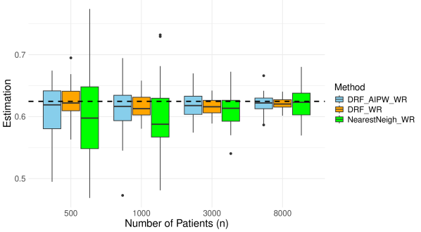
(a) $d=p=3$

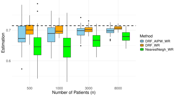
(b) $d=p=8$

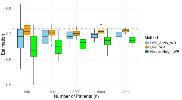
(c) $d=p=20$

Figure 2: Testing for the impact of the dimension, correlated outcomes setting. Boxplots over 100 runs. DRF AIPW WR, DRF WR and NearestNeigh WR respectively correspond to the AIPW method in Equation˜13, the direct distributional approach in Equation˜12 and the weighted Nearest Neighbor approach in Equation˜11. For the AIPW and distributional regression approach, Distributional Random Forests (DRFs, Bénard et al. (2024)) are used to perform distributional regression, using 1000 trees. For the weighted Nearest Neighbor and for the AIPW approaches, probability forests (of the GRF package) are used to estimate propensities, with 1000 trees. Propensity scores estimated with logistic regression gave comparable results.

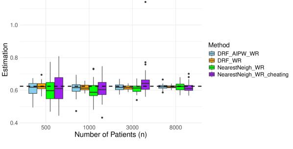
(a) $d=p=3$

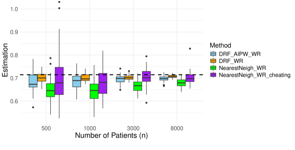
(b) $d=p=8$

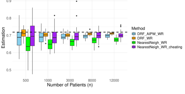
(c) $d=p=20$

Figure 3: Same setting as in Figure˜2, with an added method: Nearest Neighbor with a ‘cheating’ option, that corresponds to exactly plugging in the propensity scores instead of estimating them. Boxplots over 100 runs.

(a) $d=p=3$

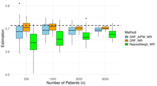
(b) $d=p=8$

(c) $d=p=20$

Figure 4: Testing for the impact of the dimension, uncorrelated outcomes setting. Boxplots over 100 runs. DRF AIPW WR, DRF WR and NearestNeigh WR as in Figure˜2

.

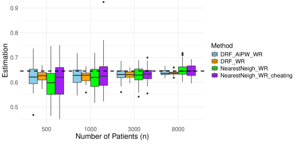
(a) $d=p=3$

(b) $d=p=8$

(c) $d=p=20$

Figure 5: Testing for the impact of the dimension, uncorrelated outcomes setting. Boxplots over 100 runs. DRF AIPW WR, DRF WR, NearestNeigh WR with and without ‘CHEATING’ option as in Figure˜3

.

5.2 Misspecification and double robustness

We next provide two synthetized experiments, to illustrate the double-robustness of our augmented estimator (Equation˜13), that respectively correspond to Figure˜6(a) and Figure˜6(b).

1. In the first experiment, we test for double robustness by mispecifying propensities. Instead of using probability forests to learn propensities, we use a linear classifier that we train using logistic regression. We generate probability of treatment non-linearly, of the form $\sigma(X_{i,1}X_{i,2})$ for some $\sigma:\mathbb{R}\to[0,1]$ (Cdf of a Gaussian, in our case). Treatment responses are then generated as multi dimensional Bernoulli random variables, of means $\sigma((X_{i,1}-X_{i,2})^{2})$ and $\sigma((X_{i,1}+X_{i,2})^{2})$ for respectively treated and non-treated individuals.

2. The second experiment tests for double robustness by mispecifying in the distributional regression. We perform distributional regression as in Section˜4.2.3 with logistic regression on the outcomes, by training as in the homogeneous setting, i.e. by imposing $u_{1}^{(t)}=\ldots=u_{p}^{(t)}$ for $t=0,1$. We generate treatment assignments and responses exactly as in Figure˜5(c) (heterogeneous setting).

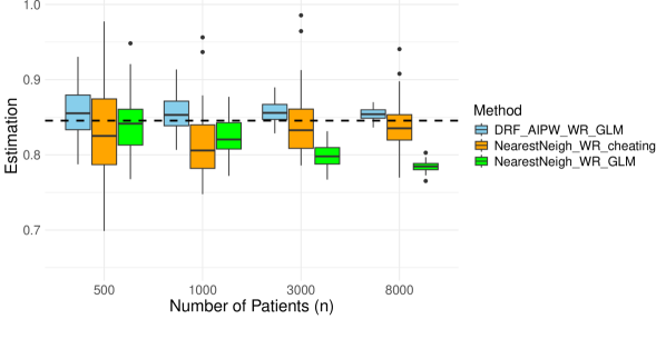
(a) Testing for robustness to mispecified propensities, $d=p=8$

(b) Testing for robustness to mispecified distributional regression, $d=p=5$

Figure 6: Testing for double robustness, by mispecifying either propensities or distributional regression.. Boxplots over 100 runs. DRF AIPW WR, DRF WR, NearestNeigh WR with as in Figure˜3, ‘mispecified’ refers to learning a linear logistic regression for propensities (Figure˜6(a)), or doing logistic distribution regression as in Section˜4.2.3 and imposing a correlated outcomes for distributional regression (fig.˜6(b)) while the outcomes are generated uncorrelated.

6 Conclusion and open directions

In this paper, we have introduced a causal inference framework for hierarchical outcome comparison methods like Win Ratio or Generalized Pairwise Comparisons. Our goal is to make such methods more grounded, by offering new perspectives and shedding light on the different causal effect measures that may be targeted when performing a Win Ratio or related analysis. In particular, we highlight the fact that if the population is heterogeneous, complete pairings (the historical and traditional way of forming pairs to compute the Win Ratio or the Net Benefit of a treatment) may target a population-level estimand that reverses treatment recommendations. The new causal effect measure $\tau_{\star}$ we introduce in Definition˜2 aims at answering this fallacy by taking into account covariate effects in the causal effect measure, thus being more robust to heterogeneous population. We stress the fact that this causal effect measure is related to stratified Win Ratio, since it can be estimated using an extreme form of stratification i.e., a Nearest Neighbors approach when forming pairs of treated-control patients. Sections˜4 and 4.2 are then devoted to the estimation of our newly introduced estimand $\tau_{\star}$, in an effort to extend hierarchical outcome analyses and the Win Ratio methodology to observational settings and to handle missing covariates. We do so using a classical inverse propensity weighting approach to generalize our Nearest Neighbor pairing method, and using a less conventional distributional regression approach, that proves to be very efficient by leveraging recent Machine Learning tools such as distribution random forests.

Finally, our work paves the way to many open directions, among which we would like to highlight one: policy learning in the presence of hierarchical outcomes, an unexplored direction in the literature. A direct byproduct of our analysis and of Definition˜2 is to define the value of a policy $\pi:\mathcal{X}\to{{\left\{0,1\right\}}}$ as:

$$V(\pi)\stackrel{{\scriptstyle\text{def}}}{{=}}\mathbb{E}\left[\tau_{\star}^{(\pi(X_{i}))}(X_{i})\right]\,,$$

where

$$\tau_{\star}^{(t)}(x)\stackrel{{\scriptstyle\text{def}}}{{=}}\mathbb{E}\left[w(Y^{(x)}(t)|Y_{i}(1-t))|X_{i}=x\right]\,.$$

An optimal treatment rule (OTR) is a policy that solves the following maximization problem:

$$\pi^{\star}\in\operatorname*{argmax}_{\pi\in\Pi}V(\pi)\,,$$

for $\Pi$ a policy set. It then appears that for unconstrained policy estimation (i.e., when $\Pi={{\left\{0,1\right\}}}^{\mathcal{X}}$), the OTR has a closed form expression that can easily be estimated using our developed tools:

$$\forall x\in\mathcal{X}\,,\quad\pi^{\star}(x)=\mathds{1}_{{\left\{\delta(x)>0\right\}}}\,,$$

where:

$$\delta(x)=\mathbb{E}\left[w(Y^{(x)}(1)|Y_{i}(0))|X_{i}=x\right]-\mathbb{E}\left[w(Y^{(x)}(0)|Y_{i}(1))|X_{i}=x\right]\,.$$

Appendix A Proof of Theorem˜1

A.1 Proof of Theorem˜1.2

Proof of Theorem˜1.2.

Let $p=\hat{p}_{W}^{(n_{0},n_{1},\mathcal{C}_{\mathrm{nn}})}=\frac{1}{n_{0}}\sum_{i\in\mathcal{N}_{0}}w(Y_{\sigma^{\star}(i)}|Y_{i})$ and $\bar{p}=\mathbb{E}\left[w(Y^{(X_{i})}(1)|Y_{i}(0))\right]$. We have, where $X_{\mathcal{N}_{1}}=(X_{k})_{k\in\mathcal{N}_{1}}$:

$$\bar{p}-p =\underbrace{\mathbb{E}\left[\frac{1}{n_{0}}\sum_{i\in\mathcal{N}_{0}}{{\left\{w(Y_{i}^{(X_{i})}(1)|Y_{i}(0))-w(Y_{\sigma^{\star}(i)}|Y_{i})\right\}}}\Big{|}X_{\mathcal{N}_{1}}\right]}_{A_{1}}$$

$$\quad+\underbrace{\frac{1}{n_{0}}\sum_{i\in\mathcal{N}_{0}}{{\left\{w(Y_{\sigma^{\star}(i)}|Y_{i})-\mathbb{E}\left[w(Y_{\sigma^{\star}(i)}|Y_{i})|i\in\mathcal{N}_{0},X_{\mathcal{N}_{1}}\right]\right\}}}}_{A_{2}}$$

Control of $A_{2}$. The term $A_{2}$ is controlled by computing variance. Let

$$a_{i}=w(Y_{\sigma^{\star}(i)}|Y_{i})-\mathbb{E}\left[w(Y_{\sigma^{\star}(i)}|Y_{i})|i\in\mathcal{N}_{0},X_{\mathcal{N}_{1}}\right]\,,$$

and note that we have $\mathbb{E}\left[a_{i}|i\in\mathcal{N}_{0},X_{\mathcal{N}_{1}}\right]=0$. Let

$$p_{k}=\mathbb{P}\left(\sigma(i)=k|X_{\mathcal{N}_{1}}\right)$$

be the (random) weights of the (random) Voronoi cells associated to elements of $X_{\mathcal{N}_{1}}$. We have, where $i\neq j\in\mathcal{N}_{0}$ are arbitrary (note that conditioned on $X_{\mathcal{N}_{1}}$, $\mathcal{N}_{0}$ is fixed):

$${\rm var\,}(A_{2}|X_{\mathcal{N}_{1}}) =\frac{{\rm var\,}(a_{i}|X_{\mathcal{N}_{1}})}{n_{0}}$$

$$\quad+\frac{n_{0}-1}{n_{0}}\Big{(}\mathbb{E}\left[a_{i}a_{j}|\sigma(i)=\sigma(j),X_{\mathcal{N}_{1}}\right]\mathbb{P}\left(\sigma(i)=\sigma(j)|X_{\mathcal{N}_{1}}\right)$$

$$\quad+\mathbb{E}\left[a_{i}a_{j}|\sigma(i)\neq\sigma(j),X_{\mathcal{N}_{1}}\right]\mathbb{P}\left(\sigma(i)\neq\sigma(j)|X_{\mathcal{N}_{1}}\right)\Big{)}$$

$$\leqslant\frac{1}{n_{0}}+\mathbb{P}\left(\sigma(i)=\sigma(j)|X_{\mathcal{N}_{1}}\right)+\frac{n_{0}-1}{n_{0}}\mathbb{E}\left[a_{i}a_{j}|\sigma(i)\neq\sigma(j),X_{\mathcal{N}_{1}}\right]\mathbb{P}\left(\sigma(i)\neq\sigma(j)|X_{\mathcal{N}_{1}}\right)\,.$$

Conditionnally on $X_{\mathcal{N}_{1}}$, $\sigma(i)$ and $\sigma(j)$ are independent random variables that assign $k$ with probability $p_{k}$. Thus, we can prove that $a_{i},a_{j}$ are negatively correlated conditionally on $\sigma(i)\neq\sigma(j)$:

$$\mathbb{E}\left[a_{i}a_{j}\mathds{1}_{{\left\{\sigma(i)\neq\sigma(j)\right\}}}|X_{\mathcal{N}_{1}}\right] =\sum_{k\neq\ell\in\mathcal{N}_{1}}p_{k}p_{\ell}\mathbb{E}\left[a_{i}a_{j}|X_{\mathcal{N}_{1}},\sigma(i)=k,\sigma(j)=\ell\right]$$

$$=\sum_{k\neq\ell\in\mathcal{N}_{1}}p_{k}p_{\ell}\mathbb{E}\left[a_{i}|X_{\mathcal{N}_{1}},\sigma(i)=k,\sigma(j)=\ell\right]\mathbb{E}\left[a_{j}|X_{\mathcal{N}_{1}},\sigma(i)=k,\sigma(j)=\ell\right]$$

$$\qquad\quad\text{since }a_{i}\perp\!\!\!\perp a_{j}|X_{\mathcal{N}_{1}},\sigma(i)=k,\sigma(j)=\ell$$

$$=\sum_{k\neq\ell\in\mathcal{N}_{1}}p_{k}p_{\ell}\mathbb{E}\left[a_{i}|X_{\mathcal{N}_{1}},\sigma(i)=k\right]\mathbb{E}\left[a_{j}|X_{\mathcal{N}_{1}},\sigma(j)=\ell\right]$$

$$=\sum_{k,\ell\in\mathcal{N}_{1}}p_{k}p_{\ell}\mathbb{E}\left[a_{i}|X_{\mathcal{N}_{1}},\sigma(i)=k\right]\mathbb{E}\left[a_{j}|X_{\mathcal{N}_{1}},\sigma(j)=\ell\right]-\sum_{k\in\mathcal{N}_{1}}p_{k}^{2}\mathbb{E}\left[a_{i}|X_{\mathcal{N}_{1}},\sigma(i)=k\right]^{2}$$

$$\leqslant\left(\sum_{k\in\mathcal{N}_{1}}p_{k}\mathbb{E}\left[a_{i}|X_{\mathcal{N}_{1}},\sigma(i)=k\right]\right)^{2}$$

$$=0\,.$$

Using $\mathbb{E}\left[a_{i}a_{j}\mathds{1}_{{\left\{\sigma(i)\neq\sigma(j)\right\}}}|X_{\mathcal{N}_{1}}\right]=\mathbb{E}\left[a_{i}a_{j}|X_{\mathcal{N}_{1}},\sigma(i)\neq\sigma(j)\right]\mathbb{P}\left(\sigma(i)\neq\sigma(j)\right)$; we thus have that:

$$\mathbb{E}\left[a_{i}a_{j}|X_{\mathcal{N}_{1}},\sigma(i)\neq\sigma(j)\right]\leqslant 0\,.$$

Thus, we have that ${\rm var\,}(A_{2}|X_{\mathcal{N}_{1}})\leqslant\frac{1}{n_{0}}+\mathbb{P}\left(\sigma(i)=\sigma(j)\right)$, and the last step of this first part of the proof is to show that $\mathbb{P}\left(\sigma(i)=\sigma(j)\right)\to 0$, the purpose of the following lemma.

Lemma 1.

We have, for $i\neq j\in\mathcal{N}_{0}$:

$$\mathbb{P}\left(\sigma(i)=\sigma(j)\right)\to 0\,.$$

Proof of Lemma˜2.

We have:

$$\mathbb{P}\left(\sigma(i)=\sigma(j)\right)=\frac{1}{n_{1}}\sum_{k\in\mathcal{N}_{1}}\mathbb{P}\left(\sigma(i)=k|\sigma(j)=k\right)\,.$$

Let $k\in\mathcal{N}_{1}$ and $x\in\mathrm{Supp}(X)$: $\forall\varepsilon>0,\mathbb{P}\left(X\in\mathcal{B}(x,\varepsilon)\right)>0$.

First case: $\mathbb{P}\left(X=x\right)=p_{x}>0$. In that case, let $N_{x}=|{{\left\{\ell\in\mathcal{N}_{1},X_{\ell}=x\right\}}}$. We have that

$$\mathbb{P}\left(\sigma(i)=k|N_{x},X_{k}=x,\sigma(j)=k\right)=\frac{1}{N_{x}}\,,$$

and $N_{x}$ is a binomial random variable of parameters $(n_{1},p_{x})$. This leads to:

$$\mathbb{P}\left(\sigma(i)=k|X_{k}=x,\sigma(j)=k\right) =\sum_{N=1}^{n_{1}}2^{-n_{1}}\frac{p_{x}^{N}(1-p_{x})^{n_{1}-N}}{N}\binom{n_{1}}{N}$$

$$=\sum_{N=1}^{n_{1}}\frac{p_{x}^{N}(1-p_{x})^{n_{1}-N}}{n_{1}+1}\binom{n_{1}+1}{N+1}$$

$$\leqslant\frac{1}{p_{x}(n_{1}+1)}\,.$$

Thus, $\mathbb{P}\left(\sigma(i)=k|X_{k}=x,\sigma(j)=k\right)\to 0$ as $n_{1}\to\infty$.

Second case: $\mathbb{P}\left(X=x\right)=0$ (no Dirac mass). Let $\delta\in(0,1)$ and let $R>\varepsilon>0$ such that $\mathbb{P}\left(X\in\mathcal{B}(x,\varepsilon)\right)<\delta$ and $\mathbb{P}\left(X\in\mathcal{B}(x,R)\right)>1-\delta$. We cover $\mathcal{B}(0,R)\setminus\mathcal{B}(0,\varepsilon)$ with $m$ balls of radius $\varepsilon/2$: $\mathcal{B}(0,R)\setminus\mathcal{B}(0,\varepsilon)\subset\bigcup_{r=1}^{m}\mathcal{B}(z_{r},\varepsilon/2)$, where $z_{r}\in\mathcal{B}(0,R)\setminus\mathcal{B}(0,\varepsilon)$. We remove all $z_{r}$ that satisfy $\mathbb{P}\left(X\in\mathcal{B}(z_{r},\varepsilon/2)\right)=0$ from this union. Let $\mathcal{E}$ be the event ${{\left\{\forall r\in[m],\exists\ell\in\mathcal{N}_{1}\setminus{{\left\{k\right\}}},X_{\ell}\in\mathcal{B}(z_{r},\varepsilon/2)\right\}}}$. We have that

$$\mathbb{P}\left(\sigma(i)=k|X_{k}=x,\sigma(j)=k,\mathcal{E}\right) \leqslant\mathbb{P}\left(X_{i}\in\mathcal{B}(x,\varepsilon)\right)$$

$$\leqslant\delta\,.$$

Then,

$$\mathbb{P}\left(\mathcal{E}^{C}\right)\leqslant \sum_{r=1}^{m}\mathbb{P}\left(\forall\ell\in\mathcal{N}_{1}\setminus{{\left\{k\right\}}},X_{\ell}\notin\mathcal{B}(z_{r},\varepsilon/2)\right)$$

$$\leqslant m(1-p_{\min})^{n_{1}-1}\,,$$

where $p_{\min}=\min_{r\in[m]}\mathbb{P}\left(X\in\mathcal{B}(z_{r},\varepsilon/2)\right)$. Thus, $\mathbb{P}\left(\mathcal{E}\right)\to 1$, and $\mathbb{P}\left(\sigma(i)=k|X_{k}=x,\sigma(j)=k\right)\leqslant 1-\mathbb{P}\left(\mathcal{E}\right)+\delta$. We can thus conclude that $\mathbb{P}\left(\sigma(i)=k|X_{k}=x,\sigma(j)=k\right)\to 0$ as $n_{1}\to\infty$.

Wrapping things up. Using $\mathbb{P}\left(\sigma(i)=k|\sigma(j)=k\right)=\int_{\mathcal{X}}\mathbb{P}\left(\sigma(i)=k|\sigma(j)=k,X_{k}=x\right){\rm d}\mathbb{P}(X_{k}=x)$, we have $\mathbb{P}\left(\sigma(i)=k|\sigma(j)=k\right)\to 0$ as $n_{1}\to\infty$, using dominated convergence. ∎

Using this, we have ${\rm var\,}(A_{2})\to 0$, leading to $A_{2}\to 0$ in probability.

Control of $A_{1}$. We now control $A_{1}$, using the continuity assumption. Using unconfoundedness:

$$\qquad\qquad|A_{1}|\leqslant\mathbb{E}\left[\delta(X_{i},X_{\sigma^{\star}(i)},Y_{i}(0))|X_{\mathcal{N}_{1}},T_{i}=0\right]\,,\qquad\text{where}$$

$$\delta(x,x^{\prime},y)\stackrel{{\scriptstyle\text{def}}}{{=}}\left|\mathbb{E}\left[w(Y_{i}^{(X_{i})}(1)|y)|X_{i}=x\right]-\mathbb{E}\left[w(Y_{j}(1)|y)|X_{j}=x^{\prime}\right]\right|\,.$$

Let $\varepsilon>0$ and $y$ fixed. Using our continuity and compactness assumptions, $x,x^{\prime}\mapsto\delta(x,x^{\prime},y)$ is uniformly continuous on $\mathcal{X}\times\mathcal{X}$, so that there exists $\eta>$ such that if ${{\left\|x-x^{\prime}\right\|}}\leqslant\eta$, we have $\delta(x,x^{\prime},y)\leqslant\varepsilon$. We are going to show that with high probability, ${{\left\|X_{i}-X_{\sigma^{\star}(i)}\right\|}}\leqslant\eta$. Using compactness of $\mathcal{X}$, there exist $u_{1},\ldots,u_{p}\in\mathcal{X}$ such that $\mathcal{X}\subset\bigcup_{k=1}^{p}\mathcal{B}(u_{k},\eta/2)$. Let $p_{k}=\mathbb{P}\left(X_{i}\in\mathcal{B}(u_{k},\eta/2)\right)$: we assume that $p_{k}>0$ for all $k$, otherwise we remove this ball and the corresponding $u_{k}$. Let $p_{\min}=\min_{k}p_{k}>0$. Let $k_{x}\in[p]$ such that $X_{i}\in\mathcal{B}(u_{k_{x}},\eta/2)$. We have, working conditionnally on $\mathcal{N}_{0},\mathcal{N}_{1},i\in\mathcal{N}_{0}$:

$$\mathbb{P}\left({{\left\|X_{i}-X_{\sigma^{\star}(i)}\right\|}}>\eta\right) \leqslant\mathbb{E}\left[\mathbb{P}\left(X_{\sigma^{\star}(i)}\notin\mathcal{B}(u_{k_{x}},\eta/2)|k_{x}\right)\right]$$

$$=\mathbb{E}\left[\mathbb{P}\left(\forall j\in\mathcal{N}_{1}\,,\,X_{j}\notin\mathcal{B}(u_{k_{x}},\eta/2)|k_{x}\right)\right]$$

$$=\mathbb{E}\left[(1-p_{k_{x}})^{n_{1}}\right]$$

$$\leqslant(1-p_{\min})^{n_{1}}$$

$$\underset{n_{1}\to\infty}{\longrightarrow}0\,.$$

This leads to:

$$\mathbb{P}\left(\delta(X_{i},X_{\sigma(i)},y)>\varepsilon\right)\leqslant(1-p_{\min})^{n_{1}}\,,$$

and thus $\mathbb{P}\left(\delta(X_{i},X_{\sigma(i)},y)\to 0\right)=1$ as $n_{1}\to\infty$, leading to $\mathbb{E}\left[\delta(X_{i},X_{\sigma(i)},Y_{i}(0))\right]\to 0$. We thus have that $\mathbb{E}\left[|A_{1}|\right]\to 0$, and thus $A_{1}\to 0$ in probability, since $|A_{1}|\leqslant 1$ almost surely. This concludes the proof. ∎

A.2 Proof of Theorem˜1.1

Proof of Theorem˜1.1.

Let $\bar{p}=\mathbb{E}\left[w(Y_{i}(1)|Y_{j}(0))\right]$ for $i\neq j$. We now prove the second point, with complete pairings. Using our assumptions, we have that

$$\mathbb{E}\left[w(Y_{i}|Y_{j})|T_{i}=1,T_{j}=0\right]=\mathbb{E}\left[w(Y_{j}(1)|Y_{i}(0))\right]\stackrel{{\scriptstyle\text{def}}}{{=}}\bar{p}\,,$$

so that

$$\mathbb{E}\left[\hat{p}_{W}^{(n_{0},n_{1},\mathcal{C}_{\mathrm{Tot}})}\right]=\bar{p}\,.$$

Since $0\leqslant w\leqslant 1$, ${\rm var\,}(w(Y_{j}|Y_{i}))\leqslant 1$, leading to:

$${\rm var\,}\left(\hat{p}_{W}^{(n_{0},n_{1},\mathcal{C}_{\mathrm{Tot}})}\right) =\frac{1}{n_{0}^{2}n_{1}^{2}}\sum_{i,i^{\prime}\in\mathcal{N}_{0},j,j^{\prime}\in\mathcal{N}_{1}}\mathbb{E}\left[(w(Y_{j}|Y_{i})-\bar{p})(w(Y_{j^{\prime}}|Y_{i^{\prime}}))\right]$$

$$=\frac{1}{n_{0}^{2}n_{1}^{2}}\sum_{i\in\mathcal{N}_{0},j\in\mathcal{N}_{1}}\mathbb{E}\left[(w(Y_{j}|Y_{i})-\bar{p})^{2}\right]$$

$$\quad+\underbrace{\frac{1}{n_{0}^{2}n_{1}^{2}}\sum_{i\neq i^{\prime}\in\mathcal{N}_{0},j,j^{\prime}\neq\mathcal{N}_{1}}\mathbb{E}\left[(w(Y_{j}|Y_{i})-\bar{p})(w(Y_{j^{\prime}}|Y_{i^{\prime}})-\bar{p})\right]}_{=0\quad\text{(independence)}}$$

$$\quad+\frac{1}{n_{0}^{2}n_{1}^{2}}\sum_{i\in\mathcal{N}_{0},j\neq j^{\prime}\in\mathcal{N}_{1}}\mathbb{E}\left[(w(Y_{j}|Y_{i})-\bar{p})(w(Y_{j^{\prime}}|Y_{i^{\prime}}))\right]$$

$$\quad+\frac{1}{n_{0}^{2}n_{1}^{2}}\sum_{i\neq i^{\prime}\in\mathcal{N}_{0},j\in\mathcal{N}_{1}}\mathbb{E}\left[(w(Y_{j}|Y_{i})-\bar{p})(w(Y_{j^{\prime}}|Y_{i^{\prime}}))\right]$$

$$\leqslant\frac{1}{n_{0}n_{1}}+\frac{1}{n_{0}}+\frac{1}{n_{1}}\,.$$

Thus, $\hat{p}_{W}^{(n_{0},n_{1},\mathcal{C}_{\mathrm{Tot}})}\longrightarrow\bar{p}$ in probability as $n_{0},n_{1}\to\infty$. ∎

Appendix B Proof of Theorem˜2

Proof.

Let

$$\hat{p}\stackrel{{\scriptstyle\text{def}}}{{=}}\frac{1}{n}\sum_{i\in\mathcal{N}_{0}}w(Y_{\sigma_{1}^{\star}(i)}|Y_{i})(1-\hat{\pi}(X_{i}))^{-1}$$

be the IPW estimator,

$$\hat{p}^{\star}\stackrel{{\scriptstyle\text{def}}}{{=}}\frac{1}{n}\sum_{i\in\mathcal{N}_{0}}w(Y_{\sigma_{1}^{\star}(i)}|Y_{i})(1-\pi(X_{i}))^{-1}$$

be the IPW estimator with oracle propensities, and $p=\tau_{\star}$ be the targeted estimand. We have:

$$\hat{p}-p=(\hat{p}-\hat{p}^{\star})+(\hat{p}^{\star}-p)\,.$$

For this first term,

$$|\hat{p}-\hat{p}^{\star}| =\left|\frac{1}{n}\sum_{i=1}^{n}(1-T_{i})w(Y_{\sigma_{1}^{\star}(i)}|Y_{i}){{\left\{(1-\hat{\pi}(X_{i}))^{-1}-(1-\pi(X_{i}))^{-1}\right\}}}\right|$$

$$\leqslant\frac{1}{n}\sum_{i=1}^{n}(1-T_{i})w(Y_{\sigma_{1}^{\star}(i)}|Y_{i})\left|(1-\hat{\pi}(X_{i}))^{-1}-(1-\pi(X_{i}))^{-1}\right|$$

$$\leqslant\frac{1}{n}\sum_{i=1}^{n}\left|(1-\hat{\pi}(X_{i}))^{-1}-(1-\pi(X_{i}))^{-1}\right|$$

$$\leqslant\frac{1}{n}\sum_{i=1}^{n}\left\{\mathds{1}_{{\left\{\hat{\pi}(X_{i})<1-\eta^{\prime}\right\}}}\left|(1-\hat{\pi}(X_{i}))^{-1}-(1-\pi(X_{i}))^{-1}\right|\right.$$

$$\qquad\qquad\left.+\mathds{1}_{{\left\{\hat{\pi}(X_{i})\geqslant 1-\eta^{\prime}\right\}}}\left|(1-\hat{\pi}(X_{i}))^{-1}-(1-\pi(X_{i}))^{-1}\right|\right\}\,,$$

for some given $0<\eta^{\prime}<\eta$. First, notice that $u\mapsto(1-u)^{-2}$ is $\eta^{{}^{\prime}-2}-$Lipschitz on $[0,1-\eta^{\prime}]$, so that:

$$\frac{1}{n}\sum_{i=1}^{n}\mathds{1}_{{\left\{\hat{\pi}(X_{i})<1-\eta^{\prime}\right\}}}\left|(1-\hat{\pi}(X_{i}))^{-1}-(1-\pi(X_{i}))^{-1}\right| \leqslant\frac{1}{n\eta^{{}^{\prime}2}}\sum_{i=1}^{n}\mathds{1}_{{\left\{\hat{\pi}(X_{i})<1-\eta^{\prime}\right\}}}\left|\hat{\pi}(X_{i})-\pi(X_{i})\right|$$

$$\leqslant\frac{1}{n\eta^{{}^{\prime}2}}\sum_{i=1}^{n}\left|\hat{\pi}(X_{i})-\pi(X_{i})\right|$$

$$=\eta^{{}^{\prime}-2}\mathbb{E}\left[\left|\hat{\pi}(X_{i})-\pi(X_{i})\right|\right]$$

$$\quad+\frac{1}{n\eta^{{}^{\prime}2}}\sum_{i=1}^{n}{{\left\{\left|\hat{\pi}(X_{i})-\pi(X_{i})\right|-\mathbb{E}\left[\left|\hat{\pi}(X_{i})-\pi(X_{i})\right|\right]\right\}}}\,.$$

Here, we have that $\mathbb{E}\left[\left|\hat{\pi}(X_{i})-\pi(X_{i})\right|\right]\to 0$ using mean consistency, while the second term converges to 0 in probability (sum of $n$ centered bounded random variables). Then, using Cauchy-Schwarz inequality,

$$\quad\frac{1}{n}\sum_{i=1}^{n}\mathds{1}_{{\left\{\hat{\pi}(X_{i})\geqslant 1-\eta^{\prime}\right\}}}\left|(1-\hat{\pi}(X_{i}))^{-1}-(1-\pi(X_{i}))^{-1}\right|$$

$$\leqslant\sqrt{\frac{1}{n}\sum_{i=1}^{n}\mathds{1}_{{\left\{\hat{\pi}(X_{i})\geqslant 1-\eta^{\prime}\right\}}}\times\frac{1}{n}\sum_{i=1}^{n}\left((1-\hat{\pi}(X_{i}))^{-1}-(1-\pi(X_{i}))^{-1}\right)^{2}}\,.$$

The first factor in the square root satisfies

$$\frac{1}{n}\sum_{i=1}^{n}\mathds{1}_{{\left\{\hat{\pi}(X_{i})\geqslant 1-\eta^{\prime}\right\}}} =\mathbb{P}\left(\hat{\pi}(X_{i})\geqslant 1-\eta^{\prime}\right)+\frac{1}{n}\sum_{i=1}^{n}\mathds{1}_{{\left\{\hat{\pi}(X_{i})\geqslant 1-\eta^{\prime}\right\}}}-\mathbb{P}\left(\hat{\pi}(X_{i})\geqslant 1-\eta^{\prime}\right)\,.$$

The first term is deterministic and converges to zero almost surely thanks to pointwise convergence and dominated convergence, while the second term converges to zero as the averaged sum of $n$ independent, centered and bounded random variables. All this leads to $\hat{p}-\hat{p}^{\star}\to 0$ in probability and almost surely.

For the second term $\hat{p}^{\star}-p$, we adapt the proof of Theorem˜1.2. We extend the defintion of $\sigma^{\star}$ to $\mathcal{N}_{1}$: for $i\in\mathcal{N}_{1}$ we have $\sigma^{\star}(i)=i$. We have, using that $p=\mathbb{E}\left[w(Y_{i}(1),Y_{i}(0))\right]=\mathbb{E}\left[\frac{1-T_{i}}{1-\pi(X_{i})}w(Y_{i}(1),Y_{i}(0))\right]$ with unconfoundedness:

$$p-\hat{p}^{\star} =\underbrace{\mathbb{E}\left[\frac{1}{n}\sum_{i\in\mathcal{N}_{0}}\frac{w(Y^{(X_{i})}(1)|Y_{i}(0))-w(Y_{\sigma^{\star}(i)}|Y_{i})}{1-\pi(X_{i})}\Big{|}X_{\mathcal{N}_{1}}\right]}_{A_{1}}$$

$$\quad-\underbrace{\frac{1}{n}\sum_{i=1}^{n}\frac{w(Y_{\sigma^{\star}(i)}|Y_{i})(1-T_{i})}{1-\pi(X_{i})}-\mathbb{E}\left[\frac{w(Y_{\sigma^{\star}(i)}|Y_{i})(1-T_{i})}{1-\pi(X_{i})}\Big{|}X_{\mathcal{N}_{1}}\right]}_{A_{2}}\,.$$

Control of $A_{2}$. The term $A_{2}$ is controlled computing its variance, as in the proof of Theorem˜1.2. Let $a_{i}=\frac{w(Y_{\sigma^{\star}(i)}|Y_{i})(1-T_{i})}{1-\pi(X_{i})}-\mathbb{E}\left[w(Y_{\sigma^{\star}(i)}|Y_{i})|X_{\mathcal{N}_{1}}\right]$. Since $\mathbb{E}\left[a_{i}\right]=0$, we have $\mathbb{E}\left[A_{2}|X_{\mathcal{N}_{1}}\right]=0$. Then, using overlap, $|a_{i}|\leqslant 1/\eta$ almost surely, so that $\mathbb{E}\left[a_{i}^{2}|\mathcal{N}_{1}\right]\leqslant 1/\eta^{2}$.

Let $p_{k}=\mathbb{P}\left(\sigma(i)=k|X_{\mathcal{N}_{1}}\right)$ be the (random) weights of the (random) Voronoi cells associated to $X_{\mathcal{N}_{1}}$. We have:

$${\rm var\,}(A_{2}|X_{\mathcal{N}_{1}}) =\frac{1}{n^{2}}\sum_{i=1}^{n}{\rm var\,}(a_{i}|X_{\mathcal{N}_{1}})$$

$$\quad+\frac{1}{n^{2}}\sum_{i\neq j}\Big{(}\mathbb{E}\left[a_{i}a_{j}|\sigma(i)=\sigma(j),X_{\mathcal{N}_{1}}\right]\mathbb{P}\left(\sigma(i)=\sigma(j)|X_{\mathcal{N}_{1}}\right)$$

$$\qquad+\mathbb{E}\left[a_{i}a_{j}|\sigma(i)\neq\sigma(j),X_{\mathcal{N}_{1}}\right]\mathbb{P}\left(\sigma(i)\neq\sigma(j)|X_{\mathcal{N}_{1}}\right)\Big{)}$$

$$\leqslant\frac{1}{\eta^{2}n}+\frac{1}{n^{2}}\sum_{i\neq j}\mathbb{P}\left(\sigma(i)=\sigma(j)|X_{\mathcal{N}_{1}}\right)+\frac{n-1}{n}\mathbb{E}\left[a_{i}a_{j}|\sigma(i)\neq\sigma(j),X_{\mathcal{N}_{1}}\right]\mathbb{P}\left(\sigma(i)\neq\sigma(j)|X_{\mathcal{N}_{1}}\right)$$

Conditionnally on $X_{\mathcal{N}_{1}}$ and on $i,j\in\mathcal{N}_{0}$, $\sigma(i),\sigma(j)$ are independent random variables that assign $k$ with probability $p_{k}$. Thus, we can prove that $a_{i},a_{j}$ are negatively correlated conditionally on $\sigma(i)\neq\sigma(j)$:

$$\mathbb{E}\left[a_{i}a_{j}\mathds{1}_{{\left\{\sigma(i)\neq\sigma(j)\right\}}}|X_{\mathcal{N}_{1}}\right] =\sum_{k\neq\ell\in\mathcal{N}_{1}}p_{k}p_{\ell}\mathbb{E}\left[a_{i}a_{j}|X_{\mathcal{N}_{1}},\sigma(i)=k,\sigma(j)=\ell\right]$$

$$=\sum_{k\neq\ell\in\mathcal{N}_{1}}p_{k}p_{\ell}\mathbb{E}\left[a_{i}|X_{\mathcal{N}_{1}},\sigma(i)=k,\sigma(j)=\ell\right]\mathbb{E}\left[a_{j}|X_{\mathcal{N}_{1}},\sigma(i)=k,\sigma(j)=\ell\right]$$

$$\qquad\quad\text{since }a_{i}\perp\!\!\!\perp a_{j}|X_{\mathcal{N}_{1}},\sigma(i)=k,\sigma(j)=\ell$$

$$=\sum_{k\neq\ell\in\mathcal{N}_{1}}p_{k}p_{\ell}\mathbb{E}\left[a_{i}|X_{\mathcal{N}_{1}},\sigma(i)=k\right]\mathbb{E}\left[a_{j}|X_{\mathcal{N}_{1}},\sigma(j)=\ell\right]$$

$$=\sum_{k,\ell\in\mathcal{N}_{1}}p_{k}p_{\ell}\mathbb{E}\left[a_{i}|X_{\mathcal{N}_{1}},\sigma(i)=k\right]\mathbb{E}\left[a_{j}|X_{\mathcal{N}_{1}},\sigma(j)=\ell\right]-\sum_{k\in\mathcal{N}_{1}}p_{k}^{2}\mathbb{E}\left[a_{i}|X_{\mathcal{N}_{1}},\sigma(i)=k\right]^{2}$$

$$\leqslant\left(\sum_{k\in\mathcal{N}_{1}}p_{k}\mathbb{E}\left[a_{i}|X_{\mathcal{N}_{1}},\sigma(i)=k\right]\right)^{2}$$

$$=0\,.$$

Thus, we have that ${\rm var\,}(A_{2})\leqslant\frac{1}{n_{0}}+\mathbb{P}\left(\sigma(i)=\sigma(j)|i,j\in\mathcal{N}_{0}\right)$ where $i\neq j$.

Lemma 2.

We have, for $i\neq j$:

$$\mathbb{P}\left(\sigma(i)=\sigma(j)|i,j\in\mathcal{N}_{0}\right)\to 0\,.$$

Proof of Lemma˜2.

First, note that we have, for any measurable set $\mathcal{S}\subset\mathcal{X}$:

$$\frac{\mathbb{P}\left(X_{i}\in\mathcal{S}|T_{i}=1\right)}{\mathbb{P}\left(X_{i}\in\mathcal{S}|T_{i}=0\right)}\in\left[\eta^{2},\frac{1}{\eta^{2}}\right]\,.$$

Indeed, we have for $t=0,1$ and measurable set $\mathcal{S}\subset\mathcal{X}$ such that $\mathbb{P}\left(X_{i}\in\mathcal{S}\right)>0$:

$$\mathbb{P}\left(X_{i}\in\mathcal{S}|T_{i}=t\right)=\frac{\mathbb{P}\left(T_{i}=t|X_{i}\in\mathcal{S}\right)}{\mathbb{P}\left(T_{i}=t\right)}\times\mathbb{P}\left(X_{i}\in\mathcal{S}\right)\,.$$

Using overlap, this leads to $\frac{\mathbb{P}\left(X_{i}\in\mathcal{S}|T_{i}=1\right)}{\mathbb{P}\left(X_{i}\in\mathcal{S}|T_{i}=0\right)}\in\left[\eta^{2},\frac{1}{\eta^{2}}\right]$. A consequence is that for all measurable $\mathcal{S}\subset\mathcal{X}$, we have $\mathbb{P}\left(X\in\mathcal{S}\right)=0\iff\mathbb{P}\left(X\in\mathcal{S}|T=0\right)=0\iff\mathbb{P}\left(X\in\mathcal{S}|T=1\right)=0$.

We have $\mathbb{P}\left(\sigma(i)=\sigma(j)\right)=\frac{1}{n_{1}}\sum_{k\in\mathcal{N}_{1}}\mathbb{P}\left(\sigma(i)=k|\sigma(j)=k\right)$. We work conditionally on $\mathcal{N}_{1},\mathcal{N}_{0}$. Note that we have $n_{0},n_{1}\to\infty$ almost surely as $n\to\infty$. Let $k\in\mathcal{N}_{1}$ and $x\in\mathrm{Supp}(X)$: $\forall\varepsilon>0,\mathbb{P}\left(X\in\mathcal{B}(x,\varepsilon)\right)>0$.

First case: $\mathbb{P}\left(X=x|T=1\right)=p_{x}>0$. In that case, let $N_{x}=|{{\left\{\ell\in\mathcal{N}_{1},X_{\ell}=x\right\}}}$. We have that

$$\mathbb{P}\left(\sigma(i)=k|N_{x},X_{k}=x,\sigma(j)=k\right)=\frac{1}{N_{x}}\,,$$

and $N_{x}$ is a binomial random variable of parameters $(n_{1},p_{x})$. This leads to:

$$\mathbb{P}\left(\sigma(i)=k|X_{k}=x,\sigma(j)=k\right) =\sum_{N=1}^{n_{1}}2^{-n_{1}}\frac{p_{x}^{N}(1-p_{x})^{n_{1}-N}}{N}\binom{n_{1}}{N}$$

$$=\sum_{N=1}^{n_{1}}\frac{p_{x}^{N}(1-p_{x})^{n_{1}-N}}{n_{1}+1}\binom{n_{1}+1}{N+1}$$

$$\leqslant\frac{1}{p_{x}(n_{1}+1)}\,.$$

Thus, $\mathbb{P}\left(\sigma(i)=k|X_{k}=x,\sigma(j)=k\right)\to 0$ as $n_{1}\to\infty$.

Second case: $\mathbb{P}\left(X=x\right)=0$. Let $\delta\in(0,1)$. Let $R>\varepsilon>0$ such that $\mathbb{P}\left(X\in\mathcal{B}(x,\varepsilon)\right)<\delta$ and $\mathbb{P}\left(X\in\mathcal{B}(x,R)\right)>1-\delta$. We cover $\mathcal{B}(0,R)\setminus\mathcal{B}(0,\varepsilon)$ with $m$ balls of radius $\varepsilon/2$: $\mathcal{B}(0,R)\setminus\mathcal{B}(0,\varepsilon)\subset\bigcup_{r=1}^{m}\mathcal{B}(z_{r},m)$, where $z_{r}\in\mathcal{B}(0,R)\setminus\mathcal{B}(0,\varepsilon)$. We remove all $z_{r}$ that satisfy $\mathbb{P}\left(X\in\mathcal{B}(z_{r},\varepsilon/2)\right)=0$ from this union. Let $\mathcal{E}$ be the event ${{\left\{\forall r\in[m],\exists\ell\in\mathcal{N}_{1}\setminus{{\left\{k\right\}}},X_{\ell}\in\mathcal{B}(z_{r},\varepsilon/2)\right\}}}$. We have that

$$\mathbb{P}\left(\sigma(i)=k|X_{k}=x,\sigma(j)=k,\mathcal{E}\right) \leqslant\mathbb{P}\left(X_{i}\in\mathcal{B}(x,\varepsilon)\right)$$

$$\leqslant\delta/\eta^{2}\,.$$

Then,

$$\mathbb{P}\left(\mathcal{E}^{C}\right)\leqslant \sum_{r=1}^{m}\mathbb{P}\left(\forall\ell\in\mathcal{N}_{1}\setminus{{\left\{k\right\}}},X_{\ell}\notin\mathcal{B}(z_{r},\varepsilon/2)\right)$$

$$\leqslant m(1-p_{\min})^{n_{1}-1}\,,$$

where $p_{\min}=\min_{r\in[m]}\mathbb{P}\left(X\in\mathcal{B}(z_{r},\varepsilon/2)|T=1\right)>0$. Thus, $\mathbb{P}\left(\mathcal{E}\right)\to 1$, and $\mathbb{P}\left(\sigma(i)=k|X_{k}=x,\sigma(j)=k\right)\leqslant 1-\mathbb{P}\left(\mathcal{E}\right)+\delta$. We can thus conclude that $\mathbb{P}\left(\sigma(i)=k|X_{k}=x,\sigma(j)=k\right)\to 0$ as $n_{1}\to\infty$.

Wrapping things up. Using $\mathbb{P}\left(\sigma(i)=k|\sigma(j)=k\right)=\int_{\mathcal{X}}\mathbb{P}\left(\sigma(i)=k|\sigma(j)=k,X_{k}=x\right){\rm d}\mathbb{P}(X_{k}=x)$, we have $\mathbb{P}\left(\sigma(i)=k|\sigma(j)=k\right)\to 0$, using dominated convergence. ∎

Using this, we have ${\rm var\,}(A_{2})\to 0$, leading to $A_{2}\to 0$ in probability.

Control of $A_{1}$. Using unconfoundedness and overlap:

$$\qquad\qquad|A_{1}|\leqslant\delta^{-1}\mathbb{E}\left[\delta(X_{i},X_{\sigma^{\star}(i)},Y_{i}(0))|X_{\mathcal{N}_{1}},T_{i}=0\right]\,,\qquad\text{where}$$

$$\delta(x,x^{\prime},y)\stackrel{{\scriptstyle\text{def}}}{{=}}\left|\mathbb{E}\left[w(Y_{i}(1)|y)|X_{i}=x\right]-\mathbb{E}\left[w(Y_{j}(1)|y)|X_{j}=x^{\prime}\right]\right|\,.$$

Let $\varepsilon>0$ and $y$ fixed. Using our continuity and compactness assumptions, $x,x^{\prime}\mapsto\delta(x,x^{\prime},y)$ is uniformly continuous on $\mathcal{X}\times\mathcal{X}$, so that there exists $\eta>$ such that if ${{\left\|x-x^{\prime}\right\|}}\leqslant\eta$, we have $\delta(x,x^{\prime},y)\leqslant\varepsilon$. We are going to show that with high probability, ${{\left\|X_{i}-X_{\sigma^{\star}(i)}\right\|}}\leqslant\eta$. Using compactness of $\mathcal{X}$, there exist $u_{1},\ldots,u_{p}\in\mathcal{X}$ such that $\mathcal{X}\subset\bigcup_{k=1}^{p}\mathcal{B}(u_{k},\eta/2)$. Let $p_{k}=\mathbb{P}\left(X_{i}\in\mathcal{B}(u_{k},\eta/2)\right)$: we assume that $p_{k}>0$ for all $k$, otherwise we remove this ball and the corresponding $u_{k}$. Let $p_{\min}=\min_{k}p_{k}>0$. Let $k_{x}\in[p]$ such that $X_{i}\in\mathcal{B}(u_{k_{x}},\eta/2)$. We have, working conditionnally on $\mathcal{N}_{0},\mathcal{N}_{1},i\in\mathcal{N}_{0}$:

$$\mathbb{P}\left({{\left\|X_{i}-X_{\sigma^{\star}(i)}\right\|}}>\eta\right) \leqslant\mathbb{E}\left[\mathbb{P}\left(X_{\sigma^{\star}(i)}\notin\mathcal{B}(u_{k_{x}},\eta/2)|k_{x}\right)\right]$$

$$=\mathbb{E}\left[\mathbb{P}\left(\forall j\in\mathcal{N}_{1}\,,\,X_{j}\notin\mathcal{B}(u_{k_{x}},\eta/2)|k_{x}\right)\right]$$

$$=\mathbb{E}\left[(1-\eta p_{k_{x}})^{n_{1}}\right]$$

$$\leqslant(1-\eta p_{\min})^{n_{1}}$$

$$\underset{n_{1}\to\infty}{\longrightarrow}0\,.$$

This leads to:

$$\mathbb{P}\left(\delta(X_{i},X_{\sigma(i)},y)>\varepsilon\right)\leqslant(1-\eta p_{\min})^{n_{1}}\,,$$

and thus $\mathbb{P}\left(\delta(X_{i},X_{\sigma(i)},y)\to 0\right)=1$ as $n_{1}\to\infty$, leading to $\mathbb{E}\left[\delta(X_{i},X_{\sigma(i)},Y_{i}(0))\right]\to 0$ using dominated convergence. We thus have that $\mathbb{E}\left[|A_{1}|\right]\to 0$, and thus $A_{1}\to 0$ in probability, since $|A_{1}|\leqslant 1$ almost surely.

∎

Appendix C Proof of Theorem˜3

Proof of Theorem˜3.

We have, for the estimator $\hat{\tau}$ defined in Equation˜12:

$$\hat{\tau}-\tau_{\star} =\frac{1}{n}\sum_{i=1}^{n}(1-T_{i})\hat{q}_{1}(X_{i},Y_{i})+T_{i}\hat{q}_{0}(X_{i},Y_{i})-\mathbb{E}\left[w(Y^{(X_{i})}(1),Y_{i}(0))\right]$$

$$=\frac{1}{n}\sum_{i=1}^{n}(1-T_{i})q_{1}(X_{i},Y_{i})+T_{i}q_{0}(X_{i},Y_{i})-\mathbb{E}\left[w(Y^{(X_{i})}(1),Y_{i}(0))\right]$$

$$\quad+\frac{1}{n}\sum_{i=1}^{n}(1-T_{i})(\hat{q}_{1}(X_{i},Y_{i})-q_{1}(X_{i},Y_{i}))+T_{i}(\hat{q}_{0}(X_{i},Y_{i})-q_{0}(X_{i},Y_{i}))\,.$$

For the first term, we have that $(1-T_{i})q_{1}(X_{i},Y_{i})+T_{i}q_{0}(X_{i},Y_{i})$ are i.i.d. bounded random variables, of mean $\mathbb{E}\left[w(Y^{(X_{i})}(1),Y_{i}(0))\right]$, so that the first sum converges almost surely to 0. We even have, using the central limit theorem, that:

$$\frac{1}{\sqrt{n}}\sum_{i=1}^{n}(1-T_{i})q_{1}(X_{i},Y_{i})+T_{i}q_{0}(X_{i},Y_{i})-\mathbb{E}\left[w(Y^{(X_{i})}(1),Y_{i}(0))\right]\underset{\mathbb{P}}{\longrightarrow}\mathcal{N}(0,\sigma_{\infty}^{2})\,,$$

where $\sigma_{\infty}^{2}={\rm var\,}\left((1-T_{i})q_{1}(X_{i},Y_{i})+T_{i}q_{0}(X_{i},Y_{i})-\mathbb{E}\left[w(Y^{(X_{i})}(1),Y_{i}(0))\right]\right)$. For the second term, we have:

$$\quad\left|\frac{1}{n}\sum_{i=1}^{n}(1-T_{i})(\hat{q}_{1}(X_{i},Y_{i})-q_{1}(X_{i},Y_{i}))+T_{i}(q_{0}(X_{i},Y_{i})-\hat{q}_{0}(X_{i},Y_{i}))\right|$$

$$\leqslant\frac{1}{n}\sum_{i=1}^{n}|\hat{q}_{1}(X_{i},Y_{i})-q_{1}(X_{i},Y_{i})|+|\hat{q}_{0}(X_{i},Y_{i})-q_{0}(X_{i},Y_{i})|$$

$$\leqslant\frac{1}{n}\sum_{i=1}^{n}(1-T_{i})\big{(}|\hat{q}_{1}(X_{i},Y_{i})-q_{1}(X_{i},Y_{i})|-\mathbb{E}\left[|\hat{q}_{1}(X_{i},Y_{i})-q_{1}(X_{i},Y_{i})||T_{i}=0\right]\big{)}$$

$$\qquad+T_{i}\big{(}|\hat{q}_{0}(X_{i},Y_{i})-q_{0}(X_{i},Y_{i})|-\mathbb{E}\left[|\hat{q}_{1}(X_{i},Y_{i})-q_{1}(X_{i},Y_{i})|T_{i}=1\right]\big{)}$$

$$\quad+\mathbb{E}\left[|\hat{q}_{1}(X_{i},Y_{i})-q_{1}(X_{i},Y_{i})||T_{i}=0\right]+\mathbb{E}\left[|\hat{q}_{0}(X_{i},Y_{i})-q_{0}(X_{i},Y_{i})||T_{i}=1\right]\,.$$

These last two terms are deterministic and converge to zero due to our assumptions. The big sum converges almost surely to zero, as the average of $n$ i.i.d. centered and bounded random variables. This leads to the consistency of our estimator. For the asymptotic normality, it remains to prove that

$$A_{i} =\frac{1}{n}\sum_{i=1}^{n}(1-T_{i})\big{(}|\hat{q}_{1}(X_{i},Y_{i})-q_{1}(X_{i},Y_{i})|-\mathbb{E}\left[|\hat{q}_{1}(X_{i},Y_{i})-q_{1}(X_{i},Y_{i})||T_{i}=0\right]\big{)}$$

$$\qquad+T_{i}\big{(}|\hat{q}_{0}(X_{i},Y_{i})-q_{0}(X_{i},Y_{i})|-\mathbb{E}\left[|\hat{q}_{1}(X_{i},Y_{i})-q_{1}(X_{i},Y_{i})|T_{i}=1\right]\big{)}$$

is $o(1/\sqrt{n})$. We have

$$\quad{\rm var\,}\left((1-T_{i})\big{(}|\hat{q}_{1}(X_{i},Y_{i})-q_{1}(X_{i},Y_{i})|-\mathbb{E}\left[|\hat{q}_{1}(X_{i},Y_{i})-q_{1}(X_{i},Y_{i})||T_{i}=0\right]\big{)}\right)$$

$$\leqslant{\rm var\,}\left(|\hat{q}_{1}(X_{i},Y_{i})-q_{1}(X_{i},Y_{i})||T_{i}=0\right)$$

$$\leqslant\mathbb{E}\left[|\hat{q}_{1}(X_{i},Y_{i})-q_{1}(X_{i},Y_{i})|^{2}|T_{i}=0\right]$$

$$\leqslant\mathbb{E}\left[|\hat{q}_{1}(X_{i},Y_{i})-q_{1}(X_{i},Y_{i})||T_{i}=0\right]\,,$$

since $|\hat{q}_{1}(X_{i},Y_{i})-q_{1}(X_{i},Y_{i})|\leqslant 1$ (these are probabilities). Thus, under ou assumption, the variance of each term of $A_{i}$ is $o(\sqrt{1/n})$. Then, $\mathbb{P}\left(|1/n\sum_{i}A_{i}|>\varepsilon/\sqrt{n}\right)\leqslant{\rm var\,}(A_{i})\to 0$. This leads to $1/n\sum_{i}A_{i}|=o_{\mathbb{P}}(1/\sqrt{n})$, and concludes the proof. ∎

Appendix D Proof of Theorem˜4

Proof of Theorem˜4.

Assume first that (i) holds. Let

$$\tau_{\mathrm{AIPW}}^{\star} \stackrel{{\scriptstyle\text{def}}}{{=}}\frac{1}{n}\sum_{i=1}^{n}{{\left\{(1-T_{i})\hat{q}_{1}(X_{i},Y_{i})-\lambda(\hat{q}_{1}(X_{i},Y_{i})-w(Y_{\sigma_{0}(i)}|Y_{i}))\frac{1-T_{i}}{(1-\pi(X_{i}))}\right\}}}$$

$$\quad+\frac{1}{n}\sum_{i=1}^{n}{{\left\{T_{i}\hat{q}_{0}(X_{i},Y_{i})-(1-\lambda)(\hat{q}_{0}(X_{i},Y_{i})-w(Y_{i}|Y_{\sigma_{1}(i)}))\frac{T_{i}}{\pi(X_{i})}\right\}}}\,.$$

We have:

$$\hat{\tau}_{\mathrm{AIPW}}-\tau_{\mathrm{AIPW}}^{\star} =\frac{\lambda}{n}\sum_{i=1}^{n}(\hat{q}_{1}(X_{i},Y_{i})-w(Y_{\sigma_{0}(i)}|Y_{i})){{\left\{\frac{1-T_{i}}{(1-\pi(X_{i}))}-\frac{1-T_{i}}{(1-\hat{\pi}(X_{i}))}\right\}}}$$

$$\quad+\frac{1-\lambda}{n}\sum_{i=1}^{n}(\hat{q}_{0}(X_{i},Y_{i})-w(Y_{i}|Y_{\sigma_{1}(i)})){{\left\{\frac{T_{i}}{\pi(X_{i})}-\frac{T_{i}}{\hat{\pi}(X_{i})}\right\}}}\,,$$

so that:

$$|\hat{\tau}_{\mathrm{AIPW}}^{\star}-\tau_{\mathrm{AIPW}}| \leqslant\frac{\lambda}{n}\sum_{i=1}^{n}\left|(\hat{q}_{1}(X_{i},Y_{i})-w(Y_{\sigma_{0}(i)}|Y_{i})){{\left\{\frac{1-T_{i}}{(1-\pi(X_{i}))}-\frac{1-T_{i}}{(1-\hat{\pi}(X_{i}))}\right\}}}\right|$$

$$\quad+\frac{1-\lambda}{n}\sum_{i=1}^{n}\left|(\hat{q}_{0}(X_{i},Y_{i})-w(Y_{i}|Y_{\sigma_{1}(i)})){{\left\{\frac{T_{i}}{\pi(X_{i})}-\frac{T_{i}}{\hat{\pi}(X_{i})}\right\}}}\right|$$

$$\leqslant\frac{\lambda}{n}\sum_{i=1}^{n}\left|\frac{1-T_{i}}{(1-\pi(X_{i}))}-\frac{1-T_{i}}{(1-\hat{\pi}(X_{i}))}\right|+\frac{1-\lambda}{n}\sum_{i=1}^{n}\left|\frac{T_{i}}{\pi(X_{i})}-\frac{T_{i}}{\hat{\pi}(X_{i})}\right|\,.$$

We showed in the proof of Theorem˜2 that this quantity converges to 0 under our assumptions. We thus are left with proving that $\tau_{\mathrm{AIPW}}^{\star}$ converges in probability towards $\tau_{\star}$.‘ We have:

$$\tau_{\mathrm{AIPW}}^{\star}-\tau_{\star} =\underbrace{\frac{\lambda}{n}\sum_{i=1}^{n}{{\left\{w(Y_{\sigma_{0}(i)}|Y_{i})\frac{1-T_{i}}{(1-\pi(X_{i}))}-\tau_{\star}\right\}}}+\frac{1-\lambda}{n}\sum_{i=1}^{n}{{\left\{w(Y_{i}|Y_{\sigma_{1}(i)})\frac{T_{i}}{\pi(X_{i})}-\tau_{\star}\right\}}}}_{(I)}$$

$$\quad+\underbrace{\frac{1}{n}\sum_{i=1}^{n}{{\left\{(1-T_{i})\hat{q}_{1}(X_{i},Y_{i})-\lambda\hat{q}_{1}(X_{i},Y_{i})\frac{1-T_{i}}{(1-\pi(X_{i}))}\right\}}}}_{(II)}$$

$$\quad+\underbrace{\frac{1}{n}\sum_{i=1}^{n}{{\left\{T_{i}\hat{q}_{0}(X_{i},Y_{i})-(1-\lambda)\hat{q}_{0}(X_{i},Y_{i})\frac{T_{i}}{\pi(X_{i})}\right\}}}}_{(III)}\,.$$

Using Theorem˜2, we directly have that $(I)$ converges in probability towards $0$. We now need to prove the same for $(II)-(III)$. We start with $(II)$. First,

$$\mathbb{E}\left[(1-T_{i})\hat{q}_{1}(X_{i},Y_{i})|\hat{q}_{1}\right] =\mathbb{P}\left(T_{i}=0\right)\mathbb{E}\left[(1-T_{i})\hat{q}_{1}(X_{i},Y_{i})|T_{i}=0,\hat{q}_{1}\right]\,,$$

$$\mathbb{E}\left[\hat{q}_{1}(X_{i},Y_{i})\frac{1-T_{i}}{(1-\pi(X_{i}))}|\hat{q}_{1}\right] =\mathbb{E}\left[(1-T_{i})\hat{q}_{1}(X_{i},Y_{i})|T_{i}=0,\hat{q}_{1}\right]\,,$$

and thus,

$$\mathbb{E}\left[(1-T_{i})\hat{q}_{1}(X_{i},Y_{i})-\lambda\hat{q}_{1}(X_{i},Y_{i})\frac{1-T_{i}}{(1-\pi(X_{i}))}|\hat{q}_{1}\right]=(\mathbb{P}\left(T_{i}=0\right)-\lambda)\mathbb{E}\left[(1-T_{i})\hat{q}_{1}(X_{i},Y_{i})|T_{i}=0,\hat{q}_{1}\right]\,.$$

Now, since each term in the sum that defines $(II)$ is bounded by $1/\eta$, we get that:

$$\mathbb{E}\left[(II)^{2}|\hat{q}_{1}\right] =(\mathbb{P}\left(T_{i}=0\right)-\lambda)^{2}\mathbb{E}\left[(1-T_{i})\hat{q}_{1}(X_{i},Y_{i})|T_{i}=0,\hat{q}_{1}\right]^{2}$$

$$\quad+\frac{{\rm var\,}\left((1-T_{i})\hat{q}_{1}(X_{i},Y_{i})-\lambda\hat{q}_{1}(X_{i},Y_{i})\frac{1-T_{i}}{(1-\pi(X_{i}))}|\hat{q}_{1}\right)}{n}$$

$$\leqslant(\mathbb{P}\left(T_{i}=0\right)-\lambda)^{2}\mathbb{E}\left[(1-T_{i})\hat{q}_{1}(X_{i},Y_{i})|T_{i}=0,\hat{q}_{1}\right]^{2}+\frac{1}{n}$$

$$\leqslant(\mathbb{P}\left(T_{i}=0\right)-\lambda)^{2}+\frac{1}{n}$$

$$\longrightarrow 0\,,$$

under our assumption on $\lambda$. The same then applies to $(III)$, concluding the proof for our first point.

Assume now that (ii) holds. Let

$$\tau_{\mathrm{AIPW}}^{*} \stackrel{{\scriptstyle\text{def}}}{{=}}\frac{1}{n}\sum_{i=1}^{n}{{\left\{(1-T_{i})q_{1}(X_{i},Y_{i})-\lambda(q_{1}(X_{i},Y_{i})-w(Y_{\sigma_{0}(i)}|Y_{i}))\frac{1-T_{i}}{(1-\hat{\pi}(X_{i}))}\right\}}}$$

$$\quad+\frac{1}{n}\sum_{i=1}^{n}{{\left\{T_{i}q_{0}(X_{i},Y_{i})-(1-\lambda)(q_{0}(X_{i},Y_{i})-w(Y_{i}|Y_{\sigma_{1}(i)}))\frac{T_{i}}{\hat{\pi}(X_{i})}\right\}}}\,.$$

We have:

$$|\hat{\tau}_{\mathrm{AIPW}}-\tau_{\mathrm{AIPW}}^{*}| \leqslant\frac{1}{n}\sum_{i=1}^{n}\left|1-T_{i}-\lambda\frac{1-T_{i}}{(1-\hat{\pi}(X_{i}))}\right||\hat{q}_{1}(X_{i},Y_{i})-q_{1}(X_{i},Y_{i})|$$

$$\quad+\frac{1}{n}\sum_{i=1}^{n}\left|T_{i}-(1-\lambda)\frac{T_{i}}{\hat{\pi}(X_{i})}\right||\hat{q}_{0}(X_{i},Y_{i})-q_{0}(X_{i},Y_{i})|$$

$$\leqslant\frac{1}{\eta^{\prime}n}\sum_{i=1}^{n}|\hat{q}_{1}(X_{i},Y_{i})-q_{1}(X_{i},Y_{i})|$$

$$\quad+\frac{1}{\eta^{\prime}n}\sum_{i=1}^{n}|\hat{q}_{0}(X_{i},Y_{i})-q_{0}(X_{i},Y_{i})|\,,$$

and we have shown in Theorem˜3 that under our assumptions, these two sums converge to 0 in probability. Hence, we are left with proving that $|\tau_{\mathrm{AIPW}}^{*}-\tau_{\star}|\to 0$.

$$|\tau_{\mathrm{AIPW}}^{*}-\tau_{\star}| \leqslant\left|\frac{1}{n}\sum_{i=1}^{n}(1-T_{i})q_{1}(X_{i},Y_{i})+\frac{1}{n}\sum_{i=1}^{n}T_{i}q_{0}(X_{i},Y_{i})-\tau_{\star}\right|$$

$$\quad+\frac{\lambda}{n}\left|\sum_{i=1}^{n}\frac{1-T_{i}}{1-\hat{\pi}(X_{i})}(q_{1}(X_{i},Y_{i})-w(Y_{\sigma_{0}(i)}|Y_{i}))\right|$$

$$\quad+\frac{1-\lambda}{n}\left|\sum_{i=1}^{n}\frac{T_{i}}{\hat{\pi}(X_{i})}(q_{0}(X_{i},Y_{i})-w(Y_{i}|Y_{\sigma_{1}(i)}))\right|\,.$$

For the first term, we already know that it converges to 0 thanks to the proof of Theorem˜3. We thus need to control the second and third sums. We have, for the second sum:

$$\frac{1}{n}\sum_{i=1}^{n}\frac{1-T_{i}}{1-\hat{\pi}(X_{i})} (q_{1}(X_{i},Y_{i})-w(Y_{\sigma_{0}(i)}|Y_{i}))=\frac{1}{n}\sum_{i=1}^{n}\frac{1-T_{i}}{1-\hat{\pi}(X_{i})}(\mathbb{E}\left[w(Y_{i}(1)|Y_{i}(0))|X_{i},Y_{i}(0)\right]-w(Y_{\sigma_{0}(i)}|Y_{i}(0)))$$

$$=\frac{1}{n}\sum_{i=1}^{n}\frac{1-T_{i}}{1-\hat{\pi}(X_{i})}(\mathbb{E}\left[w(Y_{i}^{(X_{i})}(1),Y_{i}(0))|X_{i},Y_{i}(0)\right]-\mathbb{E}\left[w(Y_{\sigma_{0}(i)}|Y_{i}(0))|X_{i},Y_{i}(0),X_{\mathcal{N}_{1}}\right])$$

$$\quad+\frac{1}{n}\sum_{i=1}^{n}\frac{1-T_{i}}{1-\hat{\pi}(X_{i})}(\mathbb{E}\left[w(Y_{\sigma_{0}(i)}|Y_{i}(0))|X_{i},Y_{i}(0),X_{\mathcal{N}_{1}}\right]-w(Y_{\sigma_{0}(i)}|Y_{i}(0)))\,.$$

Here,

$$\frac{1}{n}\sum_{i=1}^{n}\frac{1-T_{i}}{1-\hat{\pi}(X_{i})}(\mathbb{E}\left[w(Y_{\sigma_{0}(i)}|Y_{i}(0))|X_{i},Y_{i}(0),X_{\mathcal{N}_{1}}\right]-w(Y_{\sigma_{0}(i)}|Y_{i}(0)))$$

is the mean of $n$ bounded and centered random variables. These random variables are not independent, but conditionally on $X_{\mathcal{N}_{1}}$ they are. Thus, this sum converges almost surely to 0 conditionally on $X_{\mathcal{N}_{1}}$, and thus converges almost surely to 0. We now are left with controlling:

$$A\stackrel{{\scriptstyle\text{def}}}{{=}}\frac{1}{n}\sum_{i=1}^{n}\frac{1-T_{i}}{1-\hat{\pi}(X_{i})}(\mathbb{E}\left[w(Y_{i}^{(X_{i})},Y_{i}(0))|X_{i},Y_{i}(0)\right]-\mathbb{E}\left[w(Y_{\sigma_{0}(i)}|Y_{i}(0))|X_{i},Y_{i}(0),X_{\mathcal{N}_{1}}\right])\,.$$

Note that using unconfoundedness and our uniform boundedness assumption on $\hat{\pi}$:

$$\qquad\qquad|A|\leqslant\delta^{\prime-1}\mathbb{E}\left[\zeta(X_{i},X_{\sigma_{0}(i)},Y_{i}(0))|X_{\mathcal{N}_{1}},T_{i}=0\right]\,,\qquad\text{where}$$

$$\zeta(x,x^{\prime},y)\stackrel{{\scriptstyle\text{def}}}{{=}}\left|\mathbb{E}\left[w(Y_{i}^{(X_{i})}(1)|y)|X_{i}=x\right]-\mathbb{E}\left[w(Y_{j}(1)|y)|X_{j}=x^{\prime}\right]\right|\,.$$

Let $\varepsilon>0$ and $y$ fixed. Using our continuity and compactness assumptions, $x,x^{\prime}\mapsto\zeta(x,x^{\prime},y)$ is uniformly continuous on $\mathcal{X}\times\mathcal{X}$, so that there exists $\eta>$ such that if ${{\left\|x-x^{\prime}\right\|}}\leqslant\eta$, we have $\zeta(x,x^{\prime},y)\leqslant\varepsilon$. We are going to show that with high probability, ${{\left\|X_{i}-X_{\sigma_{0}(i)}\right\|}}\leqslant\eta$. Using compactness of $\mathcal{X}$, there exist $u_{1},\ldots,u_{p}\in\mathcal{X}$ such that $\mathcal{X}\subset\bigcup_{k=1}^{p}\mathcal{B}(u_{k},\eta/2)$. Let $p_{k}=\mathbb{P}\left(X_{i}\in\mathcal{B}(u_{k},\eta/2)\right)$: we assume that $p_{k}>0$ for all $k$, otherwise we remove this ball and the corresponding $u_{k}$. Let $p_{\min}=\min_{k}p_{k}>0$. Let $k_{x}\in[p]$ such that $X_{i}\in\mathcal{B}(u_{k_{x}},\eta/2)$. We have, working conditionnally on $\mathcal{N}_{0},\mathcal{N}_{1},i\in\mathcal{N}_{0}$:

$$\mathbb{P}\left({{\left\|X_{i}-X_{\sigma_{0}(i)}\right\|}}>\eta\right) \leqslant\mathbb{E}\left[\mathbb{P}\left(X_{\sigma_{0}(i)}\notin\mathcal{B}(u_{k_{x}},\eta/2)|k_{x}\right)\right]$$

$$=\mathbb{E}\left[\mathbb{P}\left(\forall j\in\mathcal{N}_{1}\,,\,X_{j}\notin\mathcal{B}(u_{k_{x}},\eta/2)|k_{x}\right)\right]$$

$$=\mathbb{E}\left[(1-\eta p_{k_{x}})^{n_{1}}\right]$$

$$\leqslant(1-\eta p_{\min})^{n_{1}}$$

$$\underset{n_{1}\to\infty}{\longrightarrow}0\,.$$

This leads to:

$$\mathbb{P}\left(\zeta(X_{i},X_{\sigma_{0}(i)},y)>\varepsilon\right)\leqslant(1-\eta p_{\min})^{n_{1}}\,,$$

and thus $\mathbb{P}\left(\zeta(X_{i},X_{\sigma(i)},y)\to 0\right)=1$ as $n_{1}\to\infty$, leading to $\mathbb{E}\left[\zeta(X_{i},X_{\sigma_{0}(i)},Y_{i}(0))\right]\to 0$ using dominated convergence. We thus have that $\mathbb{E}\left[|A|\right]\to 0$, and $A\to 0$ in probability, since $|A|\leqslant 1$ almost surely. We proceed in the same way for the remaining term:

$$\frac{1}{n}\sum_{i=1}^{n}\frac{1-T_{i}}{1-\hat{\pi}(X_{i})}(\mathbb{E}\left[w(Y_{\sigma_{0}(i)}|Y_{i}(0))|X_{i},Y_{i}(0),X_{\mathcal{N}_{1}}\right]-w(Y_{\sigma_{0}(i)}|Y_{i}(0)))\,,$$

concluding the proof. ∎

References

• drf (2020) drf: Distributional random forests, June 2020. URL http://dx.doi.org/10.32614/CRAN.package.drf.
• Ajufo et al. (2023) Ezimamaka Ajufo, Aditi Nayak, and Mandeep R. Mehra. Fallacies of using the win ratio in cardiovascular trials. JACC: Basic to Translational Science, 8(6):720–727, June 2023. ISSN 2452-302X. doi: 10.1016/j.jacbts.2023.05.004. URL http://dx.doi.org/10.1016/j.jacbts.2023.05.004.
• Athey and Wager (2021) Susan Athey and Stefan Wager. Policy learning with observational data. Econometrica, 89(1):133–161, 2021.
• Backer et al. (2024) Mickael De Backer, Manju Sengar, Vikram Mathews, Samuel Salvaggio, Vaiva Deltuvaite-Thomas, Jean-Christophe Chiem, Everardo D Saad, and Marc Buyse. Design of a clinical trial using generalized pairwise comparisons to test a less intensive treatment regimen. Clinical Trials, 21(2):180–188, 2024.
• Bénard et al. (2024) Clément Bénard, Jeffrey Näf, and Julie Josse. MMD-based variable importance for distributional random forest. In Sanjoy Dasgupta, Stephan Mandt, and Yingzhen Li, editors, Proceedings of The 27th International Conference on Artificial Intelligence and Statistics, volume 238 of Proceedings of Machine Learning Research, pages 1324–1332. PMLR, 02–04 May 2024. URL https://proceedings.mlr.press/v238/benard24a.html.
• Biau and Devroye (2015) Gérard Biau and Luc Devroye. Lectures on the nearest neighbor method, volume 246. Springer, 2015.
• Boentert et al. (2024) Matthias Boentert, Kenneth I Berger, Jordi Díaz-Manera, Mazen M Dimachkie, Alaa Hamed, Lionel Riou França, Nathan Thibault, Pragya Shukla, Jack Ishak, and J Jaime Caro. Applying the win ratio method in clinical trials of orphan drugs: an analysis of data from the comet trial of avalglucosidase alfa in patients with late-onset pompe disease. Orphanet Journal of Rare Diseases, 19(1):14, 2024.
• Buyse (2010) Marc Buyse. Generalized pairwise comparisons of prioritized outcomes in the two-sample problem. Statistics in Medicine, 29(30):3245–3257, December 2010. ISSN 1097-0258. doi: 10.1002/sim.3923. URL http://dx.doi.org/10.1002/sim.3923.
• Cevid et al. (2022) Domagoj Cevid, Loris Michel, Jeffrey Näf, Peter Bühlmann, and Nicolai Meinshausen. Distributional random forests: Heterogeneity adjustment and multivariate distributional regression. Journal of Machine Learning Research, 23(333):1–79, 2022.
• Chen et al. (2024) Ruohui Chen, Tuo Lin, Lin Liu, Jinyuan Liu, Ruifeng Chen, Jingjing Zou, Chenyu Liu, Loki Natarajan, Wan Tang, Xinlian Zhang, and Xin Tu. A doubly robust estimator for the mann whitney wilcoxon rank sum test when applied for causal inference in observational studies. Journal of Applied Statistics, page 1–25, May 2024. ISSN 1360-0532. doi: 10.1080/02664763.2024.2346357. URL http://dx.doi.org/10.1080/02664763.2024.2346357.
• Chiaruttini et al. (2024) Maria Vittoria Chiaruttini, Giulia Lorenzoni, Gaya Spolverato, and Dario Gregori. Win statistics in observational cancer research: Integrating clinical and quality-of-life outcomes. Journal of Clinical Medicine, 13(11):3272, May 2024. ISSN 2077-0383. doi: 10.3390/jcm13113272. URL http://dx.doi.org/10.3390/jcm13113272.
• Cochran (1954) William G Cochran. Some methods for strengthening the common $\chi$ 2 tests. Biometrics, 10(4):417–451, 1954.
• Colnet et al. (2024) Bénédicte Colnet, Julie Josse, Gaël Varoquaux, and Erwan Scornet. Risk ratio, odds ratio, risk difference… which causal measure is easier to generalize?, 2024. URL https://arxiv.org/abs/2303.16008.
• Diaz-Manera et al. (2021) Jordi Diaz-Manera, Priya S Kishnani, Hani Kushlaf, Shafeeq Ladha, Tahseen Mozaffar, Volker Straub, Antonio Toscano, Ans T Van der Ploeg, Kenneth I Berger, Paula R Clemens, et al. Safety and efficacy of avalglucosidase alfa versus alglucosidase alfa in patients with late-onset pompe disease (comet): a phase 3, randomised, multicentre trial. The Lancet Neurology, 20(12):1012–1026, 2021.
• Didelez and Stensrud (2021) Vanessa Didelez and Mats Julius Stensrud. On the logic of collapsibility for causal effect measures. Biometrical Journal, 64(2):235–242, February 2021. ISSN 1521-4036. doi: 10.1002/bimj.202000305. URL http://dx.doi.org/10.1002/bimj.202000305.
• Dong et al. (2018) Gaohong Dong, Junshan Qiu, Duolao Wang, and Marc Vandemeulebroecke. The stratified win ratio. Journal of biopharmaceutical statistics, 28(4):778–796, 2018.
• Fay and Li (2024) Michael P Fay and Fan Li. Causal interpretation of the hazard ratio in randomized clinical trials. Clinical Trials, 21(5):623–635, April 2024. ISSN 1740-7753. doi: 10.1177/17407745241243308. URL http://dx.doi.org/10.1177/17407745241243308.
• Gao et al. (2024) Zijun Gao, Shu Ge, and Jian Qian. Bridging multiple worlds: multi-marginal optimal transport for causal partial-identification problem. arXiv preprint arXiv:2406.07868, 2024.
• Groenwold et al. (2011) Rolf H.H. Groenwold, Karel G.M. Moons, Linda M. Peelen, Mirjam J. Knol, and Arno W. Hoes. Reporting of treatment effects from randomized trials: A plea for multivariable risk ratios. Contemporary Clinical Trials, 32(3):399–402, May 2011. ISSN 1551-7144. doi: 10.1016/j.cct.2010.12.011. URL http://dx.doi.org/10.1016/j.cct.2010.12.011.
• Guo and Ni (2022) Xiaohan Guo and Ai Ni. Contrast weighted learning for robust optimal treatment rule estimation. Statistics in Medicine, 41(27):5379–5394, September 2022. ISSN 1097-0258. doi: 10.1002/sim.9574. URL http://dx.doi.org/10.1002/sim.9574.
• Horvitz and Thompson (1952) Daniel G Horvitz and Donovan J Thompson. A generalization of sampling without replacement from a finite universe. Journal of the American statistical Association, 47(260):663–685, 1952.
• Jiřina (1959) Miloslav Jiřina. On regular conditional probabilities. Czechoslovak Mathematical Journal, 09(3):445–451, 1959. URL http://eudml.org/doc/11992.
• Lin et al. (2023) Zhenhua Lin, Dehan Kong, and Linbo Wang. Causal inference on distribution functions. Journal of the Royal Statistical Society Series B: Statistical Methodology, 85(2):378–398, 2023.
• Mann and Whitney (1947) H. B. Mann and D. R. Whitney. On a test of whether one of two random variables is stochastically larger than the other. The Annals of Mathematical Statistics, 18(1):50–60, March 1947. ISSN 0003-4851. doi: 10.1214/aoms/1177730491. URL http://dx.doi.org/10.1214/aoms/1177730491.
• Mantel and Haenszel (1959) Nathan Mantel and William Haenszel. Statistical aspects of the analysis of data from retrospective studies of disease. Journal of the national cancer institute, 22(4):719–748, 1959.
• Mao (2017) Lu Mao. On causal estimation using $u$-statistics. Biometrika, 105(1):215–220, December 2017. ISSN 1464-3510. doi: 10.1093/biomet/asx071. URL http://dx.doi.org/10.1093/biomet/asx071.
• Mao (2024) Lu Mao. Defining estimand for the win ratio: Separate the true effect from censoring. Clinical Trials, 21(5):584–594, July 2024. ISSN 1740-7753. doi: 10.1177/17407745241259356. URL http://dx.doi.org/10.1177/17407745241259356.
• Pearl (2009) Judea Pearl. Causality. Cambridge university press, 2009.
• Pocock et al. (2011) S. J. Pocock, C. A. Ariti, T. J. Collier, and D. Wang. The win ratio: a new approach to the analysis of composite endpoints in clinical trials based on clinical priorities. European Heart Journal, 33(2):176–182, September 2011. ISSN 1522-9645. doi: 10.1093/eurheartj/ehr352. URL http://dx.doi.org/10.1093/eurheartj/ehr352.
• Pocock et al. (2023) Stuart J. Pocock, João Pedro Ferreira, Timothy J. Collier, Christiane E. Angermann, Jan Biegus, Sean P. Collins, Mikhail Kosiborod, Michael E. Nassif, Piotr Ponikowski, Mitchell A. Psotka, John R. Teerlink, Jasper Tromp, John Gregson, Jonathan P. Blatchford, Cordula Zeller, and Adriaan A. Voors. The win ratio method in heart failure trials: lessons learnt from <scp>empulse</scp>. European Journal of Heart Failure, 25(5):632–641, April 2023. ISSN 1879-0844. doi: 10.1002/ejhf.2853. URL http://dx.doi.org/10.1002/ejhf.2853.
• Redfors et al. (2020) Björn Redfors, John Gregson, Aaron Crowley, Thomas McAndrew, Ori Ben-Yehuda, Gregg W Stone, and Stuart J Pocock. The win ratio approach for composite endpoints: practical guidance based on previous experience. European Heart Journal, 41(46):4391–4399, September 2020. ISSN 1522-9645. doi: 10.1093/eurheartj/ehaa665. URL http://dx.doi.org/10.1093/eurheartj/ehaa665.
• Robins et al. (1994) James M Robins, Andrea Rotnitzky, and Lue Ping Zhao. Estimation of regression coefficients when some regressors are not always observed. Journal of the American statistical Association, 89(427):846–866, 1994.
• Simpson (1951) Edward H Simpson. The interpretation of interaction in contingency tables. Journal of the Royal Statistical Society: Series B (Methodological), 13(2):238–241, 1951.
• Splawa-Neyman et al. (1990) Jerzy Splawa-Neyman, Dorota M Dabrowska, and Terrence P Speed. On the application of probability theory to agricultural experiments. essay on principles. section 9. Statistical Science, pages 465–472, 1990.
• Wagner (1982) Clifford H Wagner. Simpson’s paradox in real life. The American Statistician, 36(1):46–48, 1982.
• Wilcoxon (1945) Frank Wilcoxon. Individual comparisons by ranking methods. Biometrics Bulletin, 1(6):80, December 1945. ISSN 0099-4987. doi: 10.2307/3001968. URL http://dx.doi.org/10.2307/3001968.
• Yin et al. (2022) Anqi Yin, Ao Yuan, and Ming T. Tan. Highly robust causal semiparametric u-statistic with applications in biomedical studies. The International Journal of Biostatistics, 20(1):69–91, November 2022. ISSN 1557-4679. doi: 10.1515/ijb-2022-0047. URL http://dx.doi.org/10.1515/ijb-2022-0047.
• Zhang and Jeong (2021) Di Zhang and Jong-Hyeon Jeong. Inference on win ratio for cluster-randomized semi-competing risk data. Japanese Journal of Statistics and Data Science, 4(2):1263–1292, June 2021. ISSN 2520-8764. doi: 10.1007/s42081-021-00131-1. URL http://dx.doi.org/10.1007/s42081-021-00131-1.
• Zhang et al. (2022) Di Zhang, Stephen R. Wisniewski, and Jong-Hyeon Jeong. Causal inference on win ratio for observational data with dependent subjects, 2022. URL https://arxiv.org/abs/2212.06676.