Data-Efficient Extremum-Seeking Control Using Kernel-Based Function Approximation

Abstract

Existing extremum-seeking control (ESC) approaches typically rely on applying repeated perturbations to input parameters and performing measurements of the corresponding performance output. Performing these measurements can be costly in practical applications, e.g., due to the use of resources, making it desirable to reduce the number of performed measurements. Moreover, the required separation between the different timescales in the ESC loop typically results in slow convergence. With these challenges in mind, this work presents an approach aimed at both increasing the convergence rate and reducing the number of measurements that need to be performed. In the proposed approach, input-output data obtained during operation is used to construct online an approximation of the system’s underlying cost function. By using this approximation to perform parameter updates when a decrease in the cost can be guaranteed, instead of performing additional measurements to perform this update, more efficient use is made of the collected data. As a result, reductions in both the required number of measurements and update steps are indeed obtained. In addition, a stability analysis of the novel ESC approach is provided. The benefits of the synergy between kernel-based function approximation and standard ESC is demonstrated in simulation on a multi-input dynamical system.

, ,

1 Introduction

Extremum-seeking control (ESC) is a data-driven control approach aimed at optimizing the steady-state performance of unknown dynamical systems. Existing ESC approaches (see, e.g., Tan et al., 2010; Scheinker, 2024) are generally based on the assumption that there exists a time-invariant input-output map that uniquely relates constant system input parameters to the corresponding steady-state performance output. To optimize the steady-state performance, typically, a small perturbation signal (dither) is added to the input parameters, and the corresponding system output is measured. In this way, information about the system’s underlying input-output map, such as its gradient, is obtained that is used in an optimization algorithm to steer the input parameters to their performance-optimizing values.

To ensure stable convergence of the input parameters to a small neighborhood of their performance-optimizing values, the different timescales in the ESC loop (the system dynamics, the dither, and optimizer dynamics) should be separated such that the measured performance output remains close to its steady-state solution and the effect of measurement errors on the dynamics of the ESC is small. In classical continuous-time ESC approaches (Krstić and Wang, 2000; Tan et al., 2006, 2010; Scheinker, 2024), for example, this timescale separation is achieved by choosing the frequency of the sinusoidal dither signal sufficiently low compared to the dominant timescale of the system dynamics, and the cut-off frequencies of the high- and low-pass filters used to estimate the gradient of the input-output map via demodulation sufficiently low compared to the dither frequency. However, due to the need for this timescale separation, the convergence rate of the input parameters is typically low. Moreover, the required continuous or repeated application of dither and the required measurements of the corresponding performance output can be costly or undesirable in practical applications, e.g., due to the use of resources such as communication bandwidth or (raw) materials, or due to the transient system responses caused by the dither resulting in scrap or waste products.

To improve the convergence rate, several observer-based ESC approaches have been proposed (Ryan and Speyer, 2010; Gelbert et al., 2012; Guay and Dochain, 2015; Haring and Johansen, 2018). In these approaches, observers are used to obtain local approximations of the input-output map, which provide information about the map (and its derivatives) that is used by the optimization algorithm to adapt the system’s input parameters. The use of observers, instead of the high- and low-pass filters in the classical continuous-time ESC approaches, allows eliminating the timescale associated with the filters and improves the gradient estimate, which enhances the convergence rate of the input parameters. Other proposed approaches instead use a short window of historic data and curve fitting techniques to obtain local approximations of the input-output map (Hunnekens et al., 2014) or the system dynamics (Van Keulen et al., 2020) to estimate the gradient of the input-output map for gradient-based optimization. In Poveda et al. (2021), an approach is proposed that allows the use of both current online measured data and datasets of historic data to obtain instead a non-local approximation of the input-output map whose gradient is used as an estimate of the gradient of the input-output map. Furthermore, besides these observer and approximation-based approaches, in Poveda and Teel (2017), an approach inspired by event-triggered control is proposed in which the convergence rate in a sampled-data ESC setting is increased by sampling the system output as soon as a triggering condition is satisfied, instead of the standard approach in sampled-data ESC of using a fixed waiting time between applying the dither and measuring the corresponding performance output to ensure sufficient timescale separation (Teel and Popović, 2001; Kvaternik and Pavel, 2011; Khong et al., 2013a, b; Hazeleger et al., 2022).

While the aforementioned approaches address the issue of slow convergence in ESC, most of them still require continuous or repeated application of dither and performing measurements of the corresponding system output, which as mentioned before can be costly in practical applications. Exceptions to this are the approaches presented in Hunnekens et al. (2014) and Guay and Dochain (2015). The former approach allows dispensing of the dither signal altogether, while the latter allows dispensing of the dither in some cases. However, the stability proof presented in Hunnekens et al. (2014) is limited to static systems, and in Guay and Dochain (2015) no clear conditions are given for when the dither can be omitted. In Rodrigues et al. (2022, 2023), the issue of the costly nature of performing measurements is partially addressed by using ideas from event-triggered control to determine when to communicate input parameter updates, aimed at reducing the number of updates of the extremum-seeking controller. Using this approach, the use of communication bandwidth is reduced. However, the approach still requires continuous application of dither.

Therefore, in this work, we aim to simultaneously address the issue of slow convergence and reduce the number of input-output measurements that need to be performed. In particular, we adopt a sampled-data ESC setting as in, e.g., Teel and Popović (2001); Hazeleger et al. (2022), since this allows for possible extensions to global optimization algorithms in the future as in Khong et al. (2013a, b) for example. In this setting, we use the input-output data collected during operation of the extremum-seeking controller to construct online an approximation of the steady-state input-output map using kernel-based function approximation. When the approximation is sufficiently accurate in a region around the current optimizer state, it is used to perform a parameter update step without requiring additional inputs to be applied or measurements to be made. In this way, more efficient use is made of previously collected data, which reduces the number of measurements that need to be performed and increases the convergence rate.

In our preliminary work (Weekers et al., 2023), only optimization of static systems maps was considered. The main additional contribution of the current work is therefore the extension of this approach to the more general case of dynamical systems, including a stability proof of the presented approach. Furthermore, we derive novel conditions for assessing whether the kernel-based approximation is sufficiently accurate to be used for a parameter update step. These conditions, which are based on solving convex optimization problems, are less conservative than the closed-form expressions used in Weekers et al. (2023). Finally, we show the benefits of the proposed approach in simulation on a nonlinear dynamical system with multiple inputs.

The remainder of this paper is organized as follows. In Section 2, we introduce the considered class of dynamical systems and formulate the optimization problem that we aim to solve. In Section 3, we present the proposed approach. A stability analysis for the proposed ESC scheme is performed in Section 4. In Section 5, the approach is demonstrated by means of a simulation example. Finally, conclusions are given in Section 6. Throughout the paper, we use the following notation.

• A continuous function $\rho:\mathbb{R}_{\geq 0}\to\mathbb{R}_{\geq 0}$ is of class $\mathcal{K}$ ($\rho\in\mathcal{K}$), if it is strictly increasing, and $\rho(0)=0$. If in addition $\rho(r)\to\infty$ as $r\to\infty$, then $\rho$ is of class $\mathcal{K}_{\infty}$ ($\rho\in\mathcal{K}_{\infty}$).

• A continuous function $\beta:\mathbb{R}_{\geq 0}\times\mathbb{R}_{\geq 0}\to\mathbb{R}_{\geq 0}$ is of class $\mathcal{K}\mathcal{L}$ $(\beta\in\mathcal{K}\mathcal{L})$ if, for each fixed $t$, $\beta(\cdot,t)\in\mathcal{K}$, and, for each fixed $s$, $\beta(s,\cdot)$ is decreasing and $\beta(s,t)\to 0$ as $t\to\infty$.

• Let $\mathcal{X}$ be a Banach space with norm $\lVert\cdot\rVert$. Given any $\mathcal{Y}\subset\mathcal{X}$, and a point $x\in\mathcal{X}$, $\lVert x\rVert_{\mathcal{Y}}:=\inf_{a\in\mathcal{Y}}\,\lVert x-a\rVert$ defines the distance of $x$ to the set $\mathcal{Y}$.

• Let $\mathcal{A}+\varepsilon\bar{\mathcal{B}}:=\{x\in\mathcal{X}:\lVert x\rVert_{\mathcal{A}}\leq\varepsilon$} be the set of all points within a distance $\varepsilon$ of $\mathcal{A}$, i.e., $\mathcal{A}+\varepsilon\bar{\mathcal{B}}$, with $\bar{\mathcal{B}}$ denoting the closed unit ball, is an $\varepsilon$-neighborhood of $\mathcal{A}$.

• The superscript $(\cdot)^{+}$ denotes update steps for discrete-time systems, e.g., $\theta_{k+1}\in F(\theta_{k})$, with $k$ the discrete time index, is denoted as $\theta^{+}\in F(\theta)$.

• The identity function is denoted by ${\rm id}(\cdot)$.

2 Problem formulation

In this section, we first introduce the class of dynamical systems that we consider. Next, we formulate the optimization problem that we aim to solve, and recall a classical sampled-data extremum-seeking control approach that can be used to solve this problem.

2.1 Considered class of dynamical systems

We consider a class of nonlinear, possibly infinite-dimensional systems, according to the following definition.

Definition 1.

Let $\Sigma_{p}$ be a time-invariant system, whose state and input are denoted by $x\in\mathcal{X}$ and $\theta\in\mathbb{R}^{n_{\theta}}$, respectively. Here, $\mathcal{X}$ is a Banach space with norm $\lVert\cdot\rVert$. Given any initial state $x_{0}\in\mathcal{X}$, and any constant input $\theta\in\mathbb{R}^{n_{\theta}}$, the state trajectory of $\Sigma_{p}$ starting at $x_{0}$ with constant input $\theta$ is denoted by $x(\cdot,x_{0},\theta)$.

We adopt the following assumption for the class of systems in Definition 1.

Assumption 2.

Given a system $\Sigma_{p}$ as in Definition 1 we assume that the following statements hold:

1. For any constant input $\theta\in\mathbb{R}^{n_{\theta}}$, there exists a closed and nonempty set $\mathcal{A}(\theta)\in\mathcal{X}$ such that

   $$\underset{t\to\infty}{\lim}\,\lVert x(t,x_{0},\theta)\rVert_{\mathcal{A}(\theta)}=0,$$ (1)

   i.e., for any constant input the system’s trajectories converge to a global attractor which defines a, potentially set-valued, map $\mathcal{A}(\cdot)$ from $\mathbb{R}^{n_{\theta}}$ to subsets of $\mathcal{X}$.

2. There exists an unknown, continuous function $h:\mathcal{X}\to\mathbb{R}$ that maps the state trajectory $x(\cdot,x_{0},\theta)$ to the system output $y$, such that for any initial state $x_{0}\in\mathcal{X}$ and any constant input $\theta\in\mathbb{R}^{n_{\theta}}$

   $$y(t):=h(x(t,x_{0},\theta))$$ (2)

   with $h(x_{1})=h(x_{2})$ for any $x_{1},x_{2}\in\mathcal{A}(\theta)$. As a consequence, since $\mathcal{A}(\theta)$ is a global attractor, the unknown steady-state input-output map

   $$f(\theta):=\underset{t\to\infty}{\lim}\>h(x(t,x_{0},\theta))$$ (3)

   is well-defined for any initial state $x_{0}\in\mathcal{X}$ and any constant input $\theta\in\mathbb{R}^{n_{\theta}}$.

3. The steady-state input-output map $f(\cdot)$ is continuously differentiable and takes its (global) minimum value in a non-empty, compact set $\mathcal{C}$, i.e., $f(\theta)>f(\theta^{*})$ for all $\theta\in\mathbb{R}^{n_{\theta}}\backslash\mathcal{C}$ with $\theta^{*}\in\mathcal{C}$. Moreover, $\nabla f(\theta)=0$ if and only if $\theta\in\mathcal{C}$.

4. For any $\Delta_{\theta},\Delta_{x}\in\mathbb{R}_{>0}$, there exists an $L_{h}\in\mathbb{R}_{>0}$ such that

   $$\lVert h(x)-f(\theta)\rVert\leq L_{h}\lVert x\rVert_{\mathcal{A}(\theta)}$$ (4)

   holds for any input $\theta\in\mathbb{R}^{n_{\theta}}$ and state $x\in\mathcal{X}$ that satisfy $\lVert\theta\rVert_{\mathcal{C}}\leq\Delta_{\theta}$ and $\lVert x\rVert_{\mathcal{A}(\theta)}\leq\Delta_{x}$.

5. The map $\mathcal{A}(\cdot)$ is locally Lipschitz. That is, for any $\Delta_{\theta}\in\mathbb{R}_{>0}$, there exists an $L_{\mathcal{A}}\in\mathbb{R}_{>0}$ such that

   $$\mathcal{A}(\theta_{1})\subseteq\mathcal{A}(\theta_{2})+L_{\mathcal{A}}\lVert\theta_{1}-\theta_{2}\rVert\bar{\mathcal{B}}$$ (5)

   if $\max\{\lVert\theta_{1}\rVert_{\mathcal{C}},\,\lVert\theta_{2}\rVert_{\mathcal{C}}\}\leq\Delta_{\theta}$.

6. Given any $\epsilon_{1},\epsilon_{2},\Delta_{x},\Delta_{\theta}\in\mathbb{R}_{>0}$, there exists a time $T\in\mathbb{R}_{>0}$, called a waiting time, such that for any constant input $\theta\in\mathbb{R}^{n_{\theta}}$ and initial condition $x_{0}\in\mathcal{X}$ that satisfy $\lVert\theta\rVert_{\mathcal{C}}\leq\Delta_{\theta}$ and $\lVert x_{0}\rVert_{\mathcal{A}(\theta)}\leq\Delta_{x}$, it holds that

   $$\lVert x(t,x_{0},\theta)\rVert_{\mathcal{A}(\theta)}\leq\epsilon_{1}\lVert x_{0}\rVert_{\mathcal{A}(\theta)}+\epsilon_{2}$$ (6)

   for all $t\geq T$.

For examples of common classes of systems that satisfy Definition 1 and Assumption 2 see Khong et al. (2013b, Section 2).

Remark 3.

The class of systems satisfying Definition 1 and Assumption 2 considered here is largely in line with the classes of systems considered in, e.g., Teel and Popović (2001), Khong et al. (2013b) and Hazeleger et al. (2022). The main differences are that: (i) in those works $f(\cdot)$ is only assumed to be locally Lipschitz instead of continuously differentiable with $\nabla f(\theta)=0\Leftrightarrow\theta\in\mathcal{C}$ (the reason for the stricter assumption made here will be made clear in Section 3.1); (ii) in Khong et al. (2013b) the inputs $\theta$ are restricted to a compact subset of $\mathbb{R}^{n_{\theta}}$ while here $\theta\in\mathbb{R}^{n_{\theta}}$; and (iii) in Hazeleger et al. (2022) the system has additional outputs related to measurable constraints, while no constraints are considered here.

2.2 Problem formulation

In the context of ESC, the input $\theta$ and output $y$ of the system $\Sigma_{p}$ can be seen as a vector of tunable system parameters and a to-be-optimized performance variable, respectively. The (constant) input and the output are related in steady-state via the steady-state input-output map $f(\cdot)$ in (3), which thus represents a steady-state cost function for the system $\Sigma_{p}$. However, the system dynamics and consequentially the input-output map $f(\cdot)$ are unknown. The goal in ESC is therefore to solve the steady-state optimization problem

$$\theta^{*}:=\underset{\theta\in\mathbb{R}^{n_{\theta}}}{\text{arg min}}\>f(\theta)$$ (7)

solely on the basis of input-output data of the system $\Sigma_{p}$, i.e., only using knowledge on the applied input $\theta$ and the measured output $y$.

To solve the steady-state optimization problem (7), typical ESC approaches require the addition of small perturbations $v(\cdot)$ (called dither) to the input parameters $\theta$, and measurements of the corresponding (near steady-state) output $y$. These perturbed inputs and corresponding measured outputs are used by an optimization algorithm aimed at solving (7). Here, we will focus in particular on a class of optimization algorithms that can be described by a difference inclusion (see also, e.g., Teel and Popović (2001) and Hazeleger et al. (2022)). Extensions to a broader class of optimization algorithms, such as in Khong et al. (2013a, b) for example, are left as future work. The class of optimization algorithms that we consider can thus be described by

$$\Sigma:\quad\theta^{+}\in F(\theta,Y(\theta)),$$ (8)

where $F:\mathbb{R}^{n_{\theta}}\times\mathbb{R}^{n_{v}}\to\mathbb{R}^{n_{\theta}}$ is a set-valued map whose input-output behavior depends on tunable parameters of the optimization algorithm, and the updated parameters $\theta^{+}$ can be any element of the set. Furthermore, the map $Y:\mathbb{R}^{n_{\theta}}\to\mathbb{R}^{n_{v}}$ defined as

$$Y(\theta):=\begin{bmatrix}f(\theta+v_{1}(\theta))\\ \vdots\\ f(\theta+v_{n_{v}}(\theta))\end{bmatrix}$$ (9)

with dither functions $v_{j}(\cdot)$, $j=1,\dots,n_{v}$, and input-output map $f(\cdot)$, maps inputs $\theta$ to vectors containing information regarding (the gradient of) $f(\cdot)$ near $\theta$.

However, as mentioned before, the input-output map $f(\cdot)$ is unknown, and thus the elements of $Y(\theta)$ in (9) cannot be evaluated directly. Instead, they can only be evaluated via measurements of the system output $y$. These output measurements do not exactly match the corresponding values of $f(\cdot)$, due to the system not fully being in steady state at the moment a measurement is taken. Therefore, to analyze convergence properties of the optimization algorithm to the set of minimizers $\mathcal{C}$, and the effect that perturbations to the elements of $Y(\theta)$ in (9) have on these convergence properties, we adopt the following assumptions on the optimization algorithm (8)-(9) and the dither functions $v_{j}(\cdot)$.

Assumption 4.

Given the optimization algorithm and dither functions $v_{j}(\cdot)$ as in (8)-(9), we assume that the following statements hold:

1. For each input $\theta\in\mathbb{R}^{n_{\theta}}$, the set $F(\theta,Y(\theta))$ in (8) is nonempty and compact. Moreover, $F$ is an upper semi-continuous function of $\theta$.

2. There exists class-$\mathcal{K}_{\infty}$ functions $\omega_{1}$, $\omega_{2}$, and $\rho$, and a nonnegative constant $\delta\in\mathbb{R}_{\geq 0}$, such that, for any $\theta\in\mathbb{R}^{n_{\theta}}$ and $\theta^{*}\in\mathcal{C}$,

   $$\omega_{1}(\lVert\theta\rVert_{\mathcal{C}})\leq f(\theta)-f(\theta^{*})\leq\omega_{2}(\lVert\theta\rVert_{\mathcal{C}})$$ (10)

   and

   $$\underset{\theta^{+}\in F(\theta,Y(\theta))}{\max}\>f(\theta^{+})-f(\theta)\leq-\rho(f(\theta)-f(\theta^{*}))+\delta.$$ (11)

3. The constant $\delta\in\mathbb{R}_{\geq 0}$ in (11) can be made arbitrarily small by tuning parameters of the optimization algorithm $F$ in (8).

4. For any $\Delta_{\theta},\Delta_{Y}\in\mathbb{R}_{>0}$, there exists an $L_{Y}\in\mathbb{R}_{>0}$ such that if $\lVert\theta\rVert_{\mathcal{C}}\leq\Delta_{\theta}$ and $\lVert\widetilde{Y}(\theta)\rVert\leq\Delta_{Y}$ with $\widetilde{Y}(\theta)$ a version of $Y(\theta)$ in (9) with inexact (i.e., non-steady-state) measurements of $f(\cdot)$ (cf. (18)), then

   $$\lVert\theta_{\smash{\widetilde{F}}}-\theta_{F}\rVert\leq L_{Y}\lVert\widetilde{Y}(\theta)-Y(\theta)\rVert,$$ (12)

   where $\theta_{\smash{\widetilde{F}}}$ denotes any element of the set generated by $F(\theta,\widetilde{Y}(\theta))$, and $\theta_{F}$ denotes its closest point in the set $F(\theta,Y(\theta))$.

5. For any $\Delta_{\theta}\in\mathbb{R}_{>0}$, there exist constants $M_{v},c_{v}\in\mathbb{R}_{\geq 0}$ such that

   $$\lVert v_{j}(\theta)\rVert\leq M_{v}\lVert\theta\rVert_{\mathcal{C}}+c_{v},\quad j=1,\dots,n_{v},$$ (13)

   for any input $\theta$ such that $\lVert\theta\rVert_{\mathcal{C}}\leq\Delta_{\theta}$.

Remark 5.

Assumption 4 is largely aligned with the assumptions on the optimizer made in Teel and Popović (2001) and Hazeleger et al. (2022) (see also the remark in Khong et al. (2013b, Section 6.2) about the assumptions in Teel and Popović (2001)). The main differences are that: (i) in those works $f(\theta)-f(\theta^{*})$ in (10) and (11) is replaced by a more general locally Lipschitz function $V(\theta)$ (the reason for our stricter assumption will be made clear in Section 4); and (ii) in Hazeleger et al. (2022) additional terms are present in the assumptions that relate to measurable constraints which are not considered here.

Given these assumptions, we recall in Algorithm 1 what we will refer to as a standard parameter update step: a single iteration of the extremum-seeking control algorithm considered in, e.g., Hazeleger et al. (2022) (taking the number of constraints equal to zero) and Teel and Popović (2001). Note that each standard update step described in Algorithm 1 requires $n_{v}$ sequential experiments in which the input-output map $f(\cdot)$ is approximately evaluated for the inputs $\widetilde{\theta}_{i}$ (optimizer state plus dither) via the measured outputs $\widetilde{y}_{i}$. Furthermore, the data collected during these experiments are typically only used for a single algorithm update step, after which they are discarded.

Given the potentially costly nature of performing experiments, we present in the next section an approach for making more efficient use of the collected input-output data $\mathcal{D}_{k}=\{(\widetilde{\theta}_{i},\widetilde{y}_{i}):i=1,\dots,N_{k}\}$. In this approach, the collected data are used to construct online an approximation of the input-output map $f(\cdot)$, which, when it is sufficiently accurate in a sense that will become clear later, is used to determine a search direction and suitable optimizer gain for a gradient-based optimization step without the need for additional experiments.

Algorithm 1 Standard parameter update step

1:Waiting time $T$; number of experiments for a single algorithm update $n_{v}$; dither functions $v_{j}(\cdot)$, $j=1,\dots,n_{v}$; number of experiments performed up to the current algorithm update step $N_{k}$; and optimization algorithm state $\widehat{\theta}_{k}$, time $t_{0,k}$, and system state $x_{0,k}$ at the start of the current algorithm update step $k$.

2:Updated parameters $\widehat{\theta}_{k+1}$.

3:for $i=N_{k}+1,\dots,N_{k}+n_{v}$ do

4:   Apply a constant input including dither $v_{j}(\cdot)$ to the system for a time duration $T$, i.e., $\displaystyle\theta(t)=\widetilde{\theta}_{i}$ $\displaystyle:=\widehat{\theta}_{k}+v_{j}(\widehat{\theta}_{k})$ $\displaystyle\forall t\in[t_{0,k}+(j-1)T,\,t_{0,k}+jT)$ (14) with $j=i-N_{k}$.

5:   Sample the system output $y$ at the end of the time interval, i.e., $\displaystyle\widetilde{y}_{i}:=y(t_{0,k}+jT)=h(\widetilde{x}_{i}(\widehat{\theta}_{k})),$ (15) with $j=i-N_{k}$ and $\displaystyle\widetilde{x}_{i}(\widehat{\theta}_{k}):=x(t_{0,k}+jT,x_{0,k},\widehat{\theta}_{k}+v_{j}(\widehat{\theta}_{k})).$ (16)

6:end for

7:Use the collected samples to update the optimizer state $\widehat{\theta}_{k}$ as in (8)-(9), i.e.,

$$\widehat{\theta}_{k+1}\in F(\widehat{\theta}_{k},\widetilde{Y}(\widehat{\theta}_{k})),$$ (17)

where $\widehat{\theta}_{k+1}$ can be any element of the set and where

$$\widetilde{Y}(\widehat{\theta}_{k}):=\begin{bmatrix}\widetilde{y}_{N_{k}+1}\\ \vdots\\ \widetilde{y}_{N_{k}+n_{v}}\end{bmatrix}=\begin{bmatrix}h(\widetilde{x}_{N_{k}+1}(\widehat{\theta}_{k}))\\ \vdots\\ h(\widetilde{x}_{N_{k}+n_{v}}(\widehat{\theta}_{k}))\end{bmatrix}$$ (18)

is an approximation of $Y(\widehat{\theta}_{k})$ with $Y(\cdot)$ as in (9).

8:return $\widehat{\theta}_{k+1}$.

3 Data-efficient extremum-seeking using surrogate modeling

This section consists of three parts. In Section 3.1, we outline how an approximation of the steady-state input-output map can be used to perform a parameter update step (instead of a standard update step as in Algorithm 1) whenever a decrease in cost can be guaranteed, to reduce the number of experiments needed to optimize performance. In Section 3.2, we discuss how such approximation can be obtained from data collected during standard parameter update steps. Finally, in Section 3.3 we discuss how the bounds used to assess whether a decrease can be guaranteed are obtained and present the full approach.

3.1 Parameter updates based on cost function approximation

Suppose that a continuously differentiable approximation $m(\cdot)$ of the steady-state input-output map $f(\cdot)$ described in Section 2 is available. In case $-\nabla m(\theta)$ is a descent direction of $f(\theta)$, i.e., if

$$\nabla f(\theta)^{\intercal}\nabla m(\theta)>0,$$ (19)

an update of the form

$$\theta^{+}=\theta-\mu\nabla m(\theta)$$ (20)

guarantees a decrease in $f(\theta)$ provided that the optimizer gain $\mu\in\mathbb{R}_{>0}$ is suitably chosen. However, unlike the standard parameter update (17) in Algorithm 1, an update of the form (20) does not require additional experiments to be performed to determine the search direction. Hence, performing updates of the form (20) reduces the total number of experiments that are needed to solve the optimization problem in (7), thus saving time.

A well-known condition used in static optimization to determine if an optimizer gain $\mu$ guarantees a decrease in $f(\theta)$ during a parameter update step of the form (20) is the so-called Armijo condition (see, e.g., Nocedal and Wright (2006, Chapter 3)), given by

$$f(\theta^{+})\leq f(\theta)-c\mu\nabla f(\theta)^{\intercal}\nabla m(\theta),$$ (21)

where $\theta^{+}$ is as in (20) and $c\in(0,1)$ is a control parameter. If $-\nabla m(\theta)$ is a descent direction (cf. (19)), satisfaction of the Armijo condition (21) guarantees a decrease in $f(\theta)$ as a result of the update step, and convergence to the optimizer if it is satisfied for all update steps (provided that Assumption 2(iii) holds, cf. Remark 3). Hence, a suitable optimizer gain $\mu$ for which a decrease in $f(\theta)$ is guaranteed can for example be obtained by performing a backtracking line search until a $\mu$ is found for which (21) is satisfied.

However, in contrast to static optimization where the cost function (and its gradient) are typically known, the steady-state input-output map $f(\cdot)$ is unknown in the context of ESC, and can only be evaluated approximately by performing experiments. Moreover, its gradient $\nabla f(\cdot)$ is unavailable, and can only be approximated by performing multiple (approximate) evaluations of $f(\cdot)$. Hence, verifying satisfaction of (19) and (21) (to determine if $-\nabla m(\theta)$ is a descent direction and to find a suitable $\mu$) would require performing multiple experiments, potentially adversely affecting the benefit of performing update steps of the form (20) in the first place. Yet, suppose two bounds $\underline{b}(\theta)$ and $\overline{b}(\theta,\mu)$ are available that can be evaluated without performing experiments and that satisfy

$$\nabla f(\theta)^{\intercal}\nabla m(\theta)\geq\underline{b}(\theta)$$ (22)

and

$$f(\theta^{+})-f(\theta)+c\mu\nabla f(\theta)^{\intercal}\nabla m(\theta)\leq\overline{b}(\theta,\mu)$$ (23)

with $\theta^{+}$ as in (20). Then, guaranteed satisfaction of (19) and (21) can be verified by checking whether $\underline{b}(\theta)>0$ and $\overline{b}(\theta,\mu)\leq 0$.

Given the discussion above, Figure 1 provides an illustration of an approach aimed at reducing the total number of experiments needed to solve the optimization problem in (7) in the context of ESC, which we briefly describe next. More details will be provided in Section 3.3.

Suppose that a dataset $\mathcal{D}_{k}=\{(\widetilde{\theta}_{i},\widetilde{y}_{i}):i=1,\dots,N_{k}\}$ of $N_{k}$ inputs $\widetilde{\theta}_{i}$ and corresponding measured outputs $\widetilde{y}_{i}$, e.g., as in (14) and (15), respectively, is available. Such dataset can for example be obtained by performing a single standard parameter update step as in Algorithm 1. From $\mathcal{D}_{k}$, we construct an approximation $m_{k}(\cdot)$ of the steady-state input-output map $f(\cdot)$ using kernel-based function approximation, as we will explain in Section 3.2. For such kernel-based approximation, it is also possible to derive bounds $\underline{b}(\theta)$ and $\overline{b}(\theta,\mu)$ satisfying (22) and (23) that can be evaluated without performing additional experiments, as we will show in Section 3.3. Hence, it can be verified without additional experiments whether $-\nabla m_{k}(\theta)$ is a descent direction of $f(\theta)$ by checking whether $\underline{b}(\theta)>0$ (cf. (19) and (22)). If this is the case, we perform a backtracking line search over $\mu$ to obtain a suitable optimizer gain $\mu$ for which $\overline{b}(\theta,\mu)\leq 0$, such that the Armijo condition (21) is guaranteed to be satisfied (cf. (23)). If such $\mu$ is found, we perform the parameter update step as in (20). In case $\underline{b}(\theta)\leq 0$ or no $\mu$ satisfying $\overline{b}(\theta,\mu)\leq 0$ has been found during the line search, we instead perform a standard parameter update step as in Algorithm 1 to: (i) update the parameters $\theta$; and (ii) collect more data that are added to the dataset $\mathcal{D}_{k+1}$ to construct a new approximation $m_{k+1}(\cdot)$ during the next iteration of the ESC algorithm.

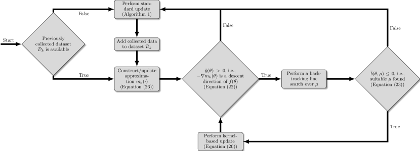
Figure 1: Block scheme illustrating kernel-based extremum-seeking control.

We will refer to the approach outlined above as kernel-based extremum-seeking control (KB-ESC). Here, ‘kernel-based’ refers to the fact that a kernel-based approximation $m_{k}(\cdot)$ of the input-output map $f(\cdot)$ is constructed and used for some parameter update steps. Furthermore, we will refer to parameter update steps as in (20) as kernel-based update steps, to distinguish them from the standard parameter update steps described in Algorithm 1.

3.2 Approximating the steady-state input-output map using kernels

Given a collected dataset $\mathcal{D}_{k}=\{(\widetilde{\theta}_{i},\widetilde{y}_{i}):i=1,\dots,N_{k}\}$ consisting of $N_{k}$ constant inputs $\widetilde{\theta}_{i}$ and corresponding measured outputs $\widetilde{y}_{i}$, e.g., as in (14) and (15), respectively, we choose to construct the approximation $m_{k}(\cdot)$ of the input-output map $f(\cdot)$ using kernel-based function approximation. We take a kernel to be a continuous, symmetric function $\kappa:\mathbb{R}^{n_{\theta}}\times\mathbb{R}^{n_{\theta}}\to\mathbb{R}$ that is positive definite according to the following definition (see, e.g., Schölkopf et al. (2001, Definition 3)).

Definition 6.

A function $\kappa:\mathbb{R}^{n_{\theta}}\times\mathbb{R}^{n_{\theta}}\to\mathbb{R}$ is called positive definite if for any $N\in\mathbb{N}$ and any set of inputs $\Omega=\{\theta_{1},\dots,\theta_{N}\}$, the $N\times N$ matrix $K_{\Omega\Omega}$, whose $(i,j)$-th element is given by $\kappa(\theta_{i},\theta_{j})$, is positive semi-definite.

By the Moore-Aronszajn theorem (Aronszajn, 1950), any kernel satisfying Definition 6 has a unique reproducing kernel Hilbert space (RKHS) of functions associated with it. This RKHS, which we will denote by $\mathcal{H}$, is the completion of the space of functions of the form $g(\cdot)=\sum_{i=1}^{N}$, $\alpha_{i}\kappa(\cdot,\theta_{i})$ with respect to the norm $\lVert g\rVert:=\sqrt{\langle g,g\rangle}$ corresponding to the inner product $\langle g_{1},g_{2}\rangle=\left\langle\sum_{i=1}^{N}\alpha_{i}\kappa(\cdot,\theta_{i}),\sum_{j=1}^{M}\beta_{j}\kappa(\cdot,\theta_{j}^{\prime})\right\rangle=\sum_{i=1}^{N}\sum_{j=1}^{M}\alpha_{i}\beta_{j}\kappa(\theta_{i},\theta_{j}^{\prime})$. Here, $N,M\in\mathbb{N}$, $\alpha_{1},\dots,\alpha_{N},\allowbreak\beta_{1},\dots,\beta_{M}\in\mathbb{R}$, and $\theta_{1},\dots,\theta_{N},\theta^{\prime}_{1},\dots,\theta^{\prime}_{M}\in\mathbb{R}^{n_{\theta}}$. Note that $\lVert g\rVert^{2}$ takes the quadratic form

$$\lVert g\rVert^{2} =\langle g,g\rangle=\left\langle\sum_{i=1}^{N}\alpha_{i}\kappa(\cdot,\theta_{i}),\sum_{j=1}^{N}\alpha_{j}\kappa(\cdot,\theta_{j})\right\rangle$$

$$=\sum_{i=1}^{N}\sum_{j=1}^{N}\alpha_{i}\alpha_{j}\kappa(\theta_{i},\theta_{j})=\alpha^{\intercal}K_{\Omega\Omega}\alpha$$ (24)

with $K_{\Omega\Omega}$ as in Definition 6 and $\alpha=[\alpha_{1}\,\cdots\,\alpha_{N}]^{\intercal}$ a vector of weights.

In order to construct an approximation $m_{k}(\cdot)$ of the steady-state input-output map $f(\cdot)$ on the basis of the dataset $\mathcal{D}_{k}$, and draw conclusions on the accuracy of the approximation, we adopt the following two assumptions whose motivation will become clear shortly (see also Scharnhorst et al. (2023, Assumptions 1 and 2)).

Assumption 7.

An upper bound $\bar{\delta}\in\mathbb{R}_{\geq 0}$ such that $\lvert f(\widetilde{\theta}_{i})-\widetilde{y}_{i}\rvert\leq\bar{\delta}$ for all measured outputs $\widetilde{y}_{i}$, $i=1,\dots,N_{k}$, is known, i.e., for every measured output $\widetilde{y}_{i}$ its distance to the corresponding steady-state value $f(\widetilde{\theta}_{i})$ is at most $\bar{\delta}$.

Assumption 8.

Given a kernel $\kappa$, the steady-state input-output map $f(\cdot)$ belongs to its corresponding RKHS $\mathcal{H}$, and an upper bound $\Gamma$ on its norm $\lVert f\rVert$ is known.

Remark 9.

Note that given Assumptions 2(iv) and 2(vi), Assumption 7 can be satisfied for any $\bar{\delta}\in\mathbb{R}_{>0}$ by choosing a sufficiently long waiting time $T$. Furthermore, the choice of kernel $\kappa$ in Assumption 8 allows including prior knowledge that might be available about the input-output map $f(\cdot)$. In case no prior knowledge about this input-output map is available, universal kernels such as the squared exponential kernel

$$\kappa(\theta,\theta^{\prime})=\exp{(-\lVert\theta-\theta^{\prime}\rVert^{2}/(2\sigma^{2}))}$$ (25)

with $\sigma$ a tunable length scale, could be chosen since such kernels have the ability to approximate any continuous function arbitrarily closely on a compact set (see, e.g., Micchelli et al. (2006)).

Given Assumptions 7 and 8, we construct the approximation $m_{k}(\cdot)$ on the basis of the dataset $\mathcal{D}_{k}$ by solving the optimization problem

$$m_{k}(\cdot)=\underset{m\in\mathcal{H}}{\rm argmin} \>\lVert m\rVert^{2}$$ (26a)

s.t. $$\>\lvert m(\widetilde{\theta}_{i})-\widetilde{y}_{i}\rvert\leq\bar{\delta}\quad\forall i\in\{1,\dots,N_{k}\},$$ (26b)

i.e., $m_{k}(\cdot)$ is the function in $\mathcal{H}$ with the smallest norm, that differs at most $\bar{\delta}$ from the data in $\mathcal{D}_{k}$.

Note that (26) is guaranteed to have a solution because the feasible set is non-empty, as by Assumptions 7 and 8 it contains the steady-state input-output map $f(\cdot)$. Moreover, note that (26) is equivalent to

$$m_{k}(\cdot)=\underset{m\in\mathcal{H}}{\rm argmin}\>\left(\lVert m\rVert^{2}+\sum_{i=1}^{N_{k}}\zeta_{\bar{\delta}}(m(\widetilde{\theta_{i}})-\widetilde{y}_{i})\right)$$ (27)

with

$$\zeta_{\bar{\delta}}(z):=\begin{cases}0,&\text{if }\lvert z\rvert\leq\bar{\delta},\\ \infty,&\text{otherwise},\end{cases}$$ (28)

which allows application of the representer theorem (Schölkopf et al., 2001, Theorem 1). The representer theorem states that the solution to (26) has the form

$$m_{k}(\cdot)=\sum_{i=1}^{N_{k}}\alpha_{i}\kappa(\cdot,\widetilde{\theta}_{i})=K_{\Omega}(\cdot)\alpha,$$ (29)

where $K_{\Omega}(\cdot):=[\kappa(\cdot,\widetilde{\theta}_{1})\,\cdots\,\kappa(\cdot,\widetilde{\theta}_{N_{k}})]$ is a row vector of kernel functions centered at the inputs $\Omega=\{\widetilde{\theta}_{1},\dots,\widetilde{\theta}_{N_{k}}\}$. Hence, substituting a solution $m(\cdot)=K_{\Omega}(\cdot)\alpha$ in (26), and using (24), we can reformulate the optimization problem as the quadratic programming problem

$$\alpha=\underset{\bar{\alpha}\in\mathbb{R}^{N_{k}}}{\rm argmin}\> \bar{\alpha}^{\intercal}K_{\Omega\Omega}\bar{\alpha}$$ (30a)

s.t. $$\lvert K_{\Omega}(\widetilde{\theta}_{i})\bar{\alpha}-\widetilde{y}_{i}\rvert\leq\bar{\delta}\quad\forall i\in\{1,\dots,N_{k}\}.$$ (30b)

As a consequence, every time a new dataset $\mathcal{D}_{k}$ is obtained by adding new data pairs $(\widetilde{\theta},\widetilde{y})$ to the previous dataset, a new approximation $m_{k}(\cdot)$ can be obtained by simply solving (30) to obtain a new weight vector $\alpha\in\mathbb{R}^{N_{k}}$ and using (29). Furthermore, since the weight vector $\alpha$ only depends on the dataset $\mathcal{D}_{k}$ and the chosen kernel $\kappa$, the gradient of the approximation $m_{k}(\cdot)$ is readily available as (cf. (29))

$$\nabla m_{k}(\cdot) =\sum_{i=1}^{N_{k}}\alpha_{i}\begin{bmatrix}D^{(e_{1},0)}\kappa(\cdot,\widetilde{\theta}_{i})&\cdots&D^{(e_{n_{\theta}},0)}\kappa(\cdot,\widetilde{\theta}_{i})\end{bmatrix}^{\intercal}$$

$$=\nabla K_{\Omega}(\cdot)\alpha$$ (31)

with $e_{i}\in\mathbb{R}^{n_{\theta}}$ a vector with $i$-th element equal to one and other elements equal to zero. In (31), we used the notation

$$D {}^{(a,b)}\kappa(\theta,\theta^{\prime})$$

$$:=\frac{\partial^{a_{1}+\cdots+a_{n_{\theta}}+b_{1}+\cdots+b_{n_{\theta}}}}{\partial\theta^{a_{1}}_{1}\cdots\partial\theta^{a_{n_{\theta}}}_{n_{\theta}}\partial(\theta^{\prime}_{1})^{b_{1}}\cdots\partial(\theta^{\prime}_{n_{\theta}})^{b_{n_{\theta}}}}\kappa(\theta,\theta^{\prime})$$ (32)

for partial derivatives of the kernel $\kappa$ (assuming that $\kappa$ is twice continuously differentiable), and

$$\nabla K_{\Omega}(\cdot):=\begin{bmatrix}D^{(e_{1},0)}\kappa(\cdot,\widetilde{\theta}_{1})&\cdots&D^{(e_{1},0)}\kappa(\cdot,\widetilde{\theta}_{N_{k}})\\ \vdots&\ddots&\vdots\\ D^{(e_{n_{\theta}},0)}\kappa(\cdot,\widetilde{\theta}_{1})&\cdots&D^{(e_{n_{\theta}},0)}\kappa(\cdot,\widetilde{\theta}_{N_{k}})\end{bmatrix}$$ (33)

denotes a matrix of partial derivatives of the kernel functions centered at the inputs $\Omega=\{\widetilde{\theta}_{1},\dots,\widetilde{\theta}_{N_{k}}\}$.

3.3 Guaranteeing a decrease in cost during kernel-based update steps

Given an approximation $m_{k}(\cdot)$ of the input-output map $f(\cdot)$ on the basis of a dataset $\mathcal{D}_{k}$ as in (26), it remains to be assessed whether a kernel-based parameter update step (20) can be performed, by studying the bounds $\underline{b}(\theta)$ and $\overline{b}(\theta,\mu)$. As explained in Section 3.1, these bounds are used to determine whether $-\nabla m_{k}(\theta)$ is a descent direction of $f(\theta)$, and to search for a suitable optimizer gain $\mu\in\mathbb{R}_{>0}$ for which the Armijo condition (21) is satisfied. We perform both these steps without requiring additional experiments to be performed. To obtain these bounds, we draw inspiration from the bounds on function values of an unknown function $f\in\mathcal{H}$ from Scharnhorst et al. (2023), that only require a dataset $\mathcal{D}_{k}$, an upper bound $\bar{\delta}$ on perturbations on the evaluations of $f(\cdot)$ as in Assumption 7, and an upper bound $\Gamma$ on $\lVert f\rVert$ as in Assumption 8. Before presenting the expressions for the bounds $\underline{b}(\theta)$ and $\overline{b}(\theta,\mu)$, for a dataset $\mathcal{D}_{k}$ we define the symmetric matrix

$$\mathfrak{K}(\theta):=\begin{bmatrix}K_{\Omega\Omega}&\nabla K_{\Omega}(\theta)^{\intercal}\\ \nabla K_{\Omega}(\theta)&D^{2}_{1,2}\kappa(\theta,\theta)\end{bmatrix}$$ (34)

with $K_{\Omega\Omega}$ the $N_{k}\times N_{k}$ matrix whose $(i,j)$-th element is given by $\kappa(\widetilde{\theta}_{i},\widetilde{\theta}_{j})$ (cf. Definition 6), $\nabla K_{\Omega}(\theta)$ a matrix of partial derivatives of the kernel functions as in (33), and

$$D^{2}_{1,2} \kappa(\theta,\theta):=$$

$$\begin{bmatrix}D^{(e_{1},e_{1})}\kappa(\theta,\theta)&\cdots&D^{(e_{1},e_{n_{\theta}})}\kappa(\theta,\theta)\\ \vdots&\ddots&\vdots\\ D^{(e_{n_{\theta}},e_{1})}\kappa(\theta,\theta)&\cdots&D^{(e_{n_{\theta}},e_{n_{\theta}})}\kappa(\theta,\theta)\end{bmatrix}$$ (35)

a matrix of second-order partial derivatives with $D^{(e_{i},e_{j})}\kappa(\theta,\theta)$ as in (32). Moreover, we define the symmetric matrix

$$\mathfrak{K}^{\prime} (\theta,\theta^{+}):=$$

$$\begin{bmatrix}K_{\Omega\Omega}&K_{\Omega}(\theta)^{\intercal}&K_{\Omega}(\theta^{+})^{\intercal}&\nabla K_{\Omega}(\theta)^{\intercal}\\ K_{\Omega}(\theta)&\kappa(\theta,\theta)&\kappa(\theta,\theta^{+})&\nabla K(\theta,\theta)^{\intercal}\\ K_{\Omega}(\theta^{+})&\kappa(\theta^{+},\theta)&\kappa(\theta^{+},\theta^{+})&\nabla K(\theta,\theta^{+})^{\intercal}\\ \nabla K_{\Omega}(\theta)&\nabla K(\theta,\theta)&\nabla K(\theta,\theta^{+})&D^{2}_{1,2}\kappa(\theta,\theta)\end{bmatrix}$$ (36)

with $K_{\Omega}(\cdot)$ a row vector of kernel functions centered at the inputs $\Omega=\{\widetilde{\theta}_{1},\dots,\widetilde{\theta}_{N_{k}}\}$ as in (29), and where

$$\nabla K(a,b):=\begin{bmatrix}D^{(e_{1},0)}\kappa(a,b)&\cdots&D^{(e_{n_{\theta}},0)}\kappa(a,b)\end{bmatrix}^{\intercal}.$$ (37)

Note that $\mathfrak{K}^{\prime}(\theta,\theta^{+})$ in (36) is what we obtain if $\mathfrak{K}(\theta)$ in (34) gets appended with evaluations of the kernel (derivatives) at $\theta$ and $\theta^{+}$, i.e., if $\Omega$ in (34) gets replaced by $\Omega^{\prime}:=\Omega\cup\{\theta,\theta^{+}\}$.

Given the definitions (34) and (36), the following theorem states that each bound $\underline{b}(\theta)$ and $\overline{b}(\theta,\mu)$ can be evaluated by solving a second-order cone program (SOCP) for a given input $\theta\in\mathbb{R}^{n_{\theta}}$ and optimizer gain $\mu\in\mathbb{R}_{>0}$.

Theorem 10.

Suppose Assumptions 7 and 8 hold. Let a dataset $\mathcal{D}_{k}=\{(\widetilde{\theta}_{i},\widetilde{y}_{i}):i=1,\dots,N_{k}\}$ of constant inputs $\widetilde{\theta}_{i}$ and corresponding output measurements $\widetilde{y}_{i}$, e.g., as in (14) and (15), respectively, be given. Furthermore, let $m_{k}(\cdot)$ be an approximation of the input-output map $f(\cdot)$ on the basis of this dataset $\mathcal{D}_{k}$ as in (26). Then the minimum value that $\nabla f(\theta)^{\intercal}\nabla m_{k}(\theta)$ can obtain at a given input $\theta\in\mathbb{R}^{n_{\theta}}$ can be found by solving the SOCP

$$\underline{b}(\theta)=$$

$$\underset{\beta\in\mathbb{R}^{N}}{\min}\> \begin{bmatrix}0_{1\times N_{k}}&\nabla m_{k}(\theta)^{\intercal}\end{bmatrix}\mathfrak{K}(\theta)\beta$$ (38a)

$${\rm s.t.}\> \beta^{\intercal}\mathfrak{K}(\theta)\beta\leq\Gamma^{2}$$ (38b)

$$\lvert\xi_{i}^{\intercal}\mathfrak{K}(\theta)\beta-\widetilde{y}_{i}\rvert\leq\overline{\delta}\quad\forall i\in\{1,\dots,N_{k}\},$$ (38c)

with $N=N_{k}+n_{\theta}$, $\mathfrak{K}(\theta)$ as in (34) and $\xi_{i}\in\mathbb{R}^{N}$ a vector with $i$-th element equal to one and other elements equal to zero.

Moreover, for any given $\mu\in\mathbb{R}_{>0}$ and $c\in(0,1)$, the maximum value that $f(\theta^{+})-f(\theta)+c\mu\nabla f(\theta)^{\intercal}\nabla m_{k}(\theta)$ with $\theta^{+}$ as in (20) can obtain at a given input $\theta\in\mathbb{R}^{n_{\theta}}$ can be found by solving the SOCP

$$\overline{b}(\theta, \mu)=$$

$$\underset{\beta\in\mathbb{R}^{N}}{{\rm max}}\> \begin{bmatrix}0_{1\times N_{k}}&-1&1&c\mu\nabla m_{k}(\theta)^{\intercal}\end{bmatrix}\mathfrak{K}^{\prime}(\theta,\theta^{+})\beta$$ (39a)

$${\rm s.t.}\> \beta^{\intercal}\mathfrak{K}^{\prime}(\theta,\theta^{+})\beta\leq\Gamma^{2}$$ (39b)

$$\lvert\xi_{i}^{\intercal}\mathfrak{K}^{\prime}(\theta,\theta^{+})\beta-\widetilde{y}_{i}\rvert\leq\overline{\delta}\quad\forall i\in\{1,\dots,N_{k}\}$$ (39c)

with $N=N_{k}+2+n_{\theta}$, $\mathfrak{K}^{\prime}(\theta,\theta^{+})$ as in (36), and $\xi_{i}\in\mathbb{R}^{N}$ again a vector with $i$-th element equal to one and other elements equal to zero.

The proof of Theorem 10 can be found in Appendix A. $\square$

Remark 11.

The inputs $\Theta=[\widetilde{\theta}_{1}\,|\,\cdots\,|\,\widetilde{\theta}_{N_{k}}\,|\,\theta\,|\,\theta^{+}]$ used in (38) and (39) might not be pairwise distinct, potentially causing the solutions to the SOCPs to be non-unique. Therefore, in case $\Theta_{i}=\Theta_{j}$, $i\neq j$, with $\Theta_{i}$ and $\Theta_{j}$ denoting the $i$-th and $j$-th column of $\Theta$, respectively, one removes the rows and columns corresponding to $\Theta_{i}$ from (38) and/or (39) to maintain uniqueness of the solution. This follows from the observation that in the proof of Theorem 10 removing $\kappa(\cdot,\Theta_{i})$ from the span in (51) does not change $\mathcal{H}^{\parallel}$ (the finite-dimensional subspace of $\mathcal{H}$ spanned by the kernel slices and their partial derivatives evaluated at the inputs in $\Theta$).

With the bounds $\underline{b}(\theta)$ and $\overline{b}(\theta,\mu)$ as in Theorem 10, we are ready to state in Algorithm 2 the proposed kernel-based extremum-seeking control algorithm that was briefly outlined in Section 3.1 (see also Figure 1). In this algorithm, we perform the backtracking line search over $\mu\in[\underline{\mu},\overline{\mu}]$ with $\underline{\mu}$ and $\overline{\mu}$ a positive lower and upper bound, respectively, by multiplying $\mu$ by a reduction factor $\varrho\in(0,1)$ until the Armijo condition (21) is guaranteed to be satisfied or $\mu<\underline{\mu}$.

Algorithm 2 Kernel-based extremum-seeking control

1:Waiting time $T$ and number of experiments $n_{v}$ for a single standard parameter update step as in Algorithm 1; upper bound $\bar{\delta}$ on the measurement perturbations as in Assumption 7; upper bound $\Gamma$ on $\lVert f\rVert$ as in Assumption 8; backtracking line search lower bound $\underline{\mu}$, upper bound $\overline{\mu}$ and reduction factor $\varrho\in(0,1)$; control parameter $c\in(0,1)$ as in the Armijo condition (21); maximum number of update steps $\bar{k}$; initial optimization algorithm state $\widehat{\theta}_{0}$; and a dataset $\mathcal{D}_{0}$ that is either empty, or contains previously obtained input-output data pairs $(\widetilde{\theta},\widetilde{y})$, e.g., as in (14)-(15).

2:Found optimal parameters $\widehat{\theta}_{\bar{k}}$.

3:Initialize the algorithm update index $k$, i.e, $k\leftarrow 0$.

4:if $\mathcal{D}_{0}$ is empty then

5:   Perform a standard parameter update step as described in Algorithm 1 to update the optimizer state $\widehat{\theta}_{0}$.

6:   Add data collected during the update step to a dataset $\mathcal{D}_{1}$, i.e., $\mathcal{D}_{1}\leftarrow\{(\widetilde{\theta}_{i},\widetilde{y}_{i}):i=1,\dots,n_{v}\}$.

7:  Update the algorithm update index $k$, i.e, $k\leftarrow 1$.

8:end if

9:while $k<\bar{k}$ do

10:   Construct an approximation $m_{k}(\cdot)$ of the input-output map $f(\cdot)$ from $\mathcal{D}_{k}$ as in (26).

11:   if $-\nabla m_{k}(\widehat{\theta}_{k})$ is guaranteed to be a descent direction of $f(\cdot)$, i.e., if $\underline{b}(\widehat{\theta}_{k})>0$ with $\underline{b}(\cdot)$ as in (38) (cf. (22)) then

12:     Perform a backtracking line search over $\mu\in[\underline{\mu},\overline{\mu}]$, i.e., set $\mu\leftarrow\overline{\mu}$ and

13:     while $\mu\geq\underline{\mu}$ and $\overline{b}(\widehat{\theta}_{k},\mu)>0$ with $\overline{b}(\cdot,\mu)$ as in (39)

14:      Reduce $\mu$, i.e., $\mu\leftarrow\varrho\mu$.

15:     end while

16:     if the Armijo condition (21) is guaranteed to be satisfied, i.e., if $\overline{b}(\widehat{\theta}_{k},\mu)\leq 0$ (cf. (23)) then

17:      Perform a kernel-based update (20) without performing additional experiments, i.e., $\widehat{\theta}_{k+1}\leftarrow\widehat{\theta}_{k}-\mu\nabla m_{k}(\widehat{\theta}_{k})$, $\mathcal{D}_{k+1}\leftarrow\mathcal{D}_{k}$, and $N_{k+1}\leftarrow N_{k}$.

18:     else

19:      Jump to Line 22.

20:     end if

21:  else

22:     Perform a standard parameter update step as described in Algorithm 1 to update the optimizer state $\widehat{\theta}_{k}$.

23:     Add data collected during the update step to a dataset $\mathcal{D}_{k+1}$, i.e., $\mathcal{D}_{k+1}\leftarrow\mathcal{D}_{k}\cup\{(\widetilde{\theta}_{i},\widetilde{y}_{i}):i=N_{k}+1,\dots,N_{k}+n_{v}\}$ and $N_{k+1}\leftarrow N_{k}+n_{v}$.

24:  end if

25:   Update the algorithm update index, i.e., $k\leftarrow k+1$.

26:end while

27:return $\widehat{\theta}_{\bar{k}}$.

4 Stability analysis for kernel-based extremum-seeking control

In this section, we perform a stability analysis for the kernel-based extremum-seeking approach described in Algorithm 2. To this end, we define for any input $\theta\in\mathbb{R}^{n_{\theta}}$ and any minimizer $\theta^{*}\in\mathcal{C}$ of $f(\theta)$ the function

$$V(\theta):=f(\theta)-f(\theta^{*}).$$ (40)

Furthermore, given this $V(\cdot)$, we define the function (see also Hazeleger et al. (2022, Equation (22)))

$$W(\psi,x,\theta):=V_{p}(\psi,x)+2V(\theta),$$ (41)

where

$$V_{p}(\psi,x):=\lVert x\rVert_{\mathcal{A}(\psi+v_{n_{v}}(\psi))}+\eta\lVert\psi\rVert_{\mathcal{C}}$$ (42)

with $\eta\in\mathbb{R}_{>0}$ a constant, $x$ the system state, and $\psi$ a memory state for the optimizer state at the start of the last standard update step. That is, $\widetilde{\theta}_{N_{k}}=\psi+v_{n_{v}}(\psi)$ is the last input that has been applied to the system (cf. (14) and Lines 5 and 22 of Algorithm 2). Note that in (41), $V_{p}(\psi,x)$ contains terms relating to the distance of the system state to the attractor $\mathcal{A}(\psi+v_{n_{v}}(\psi))$ (cf. Assumption 2(i)) corresponding to the last applied input $\psi+v_{n_{v}}(\psi)$, and the distance from the corresponding optimizer state $\psi$ to the set of minimizers $\mathcal{C}$ (cf. (42)). That is, $V_{p}(\psi,x)$ is small if the system state $x$ is close to the attractor corresponding to the last applied input and the corresponding optimizer state $\psi$ is close to the set of minimizers $\mathcal{C}$, whereas $V(\theta)$ in (41) relates to the distance of the current optimizer state $\theta$ to the set of minimizers $\mathcal{C}$ since $\omega_{1}(\lVert\theta\rVert_{\mathcal{C}})\leq V(\theta)\leq\omega_{2}(\lVert\theta\rVert_{\mathcal{C}})$ (cf. (40) and Assumption 10). Thus, $W(\psi,x,\theta)$ is small when both the current optimizer state $\theta$ and memory state $\psi$ are close to $\mathcal{C}$, and $x$ is close to the attractor corresponding to the last applied input $\psi+v_{n_{v}}(\psi)$.

The following two lemmas state that there exist upper bounds on the increment

$$\Delta W(\psi,x,\theta) :=W(\psi^{+},x^{+},\theta^{+})-W(\psi,x,\theta)$$ (43)

during standard update steps, and the increment

$$\Delta V(\theta) :=V(\theta^{+})-V(\theta)$$ (44)

during kernel-based update steps, respectively, which will prove to be useful in the stability analysis.

Lemma 12.

Suppose that the system $\Sigma_{p}$ in Definition 1 satisfies Assumption 2, and that the optimization algorithm $\Sigma$ in (8) satisfies Assumption 4. Let $x$ and $\theta$ denote, respectively, the state of $\Sigma_{p}$ and $\Sigma$ at the start of the current algorithm update step $k$. Furthermore, let $\psi$ denote a memory state for optimizer state at the start of the last standard update step, i.e., $\widetilde{\theta}_{N_{k}}=\psi+v_{n_{v}}(\psi)$ is the last input that has been applied to the system (cf. (14)). Then, for any $\Delta_{\theta},\Delta_{x}\in\mathbb{R}_{>0}$ such that $\lVert\theta\rVert_{\mathcal{C}}\leq\Delta_{\theta}$, $\lVert\psi\rVert\leq\Delta_{\theta}$, and $\lVert x\rVert_{\mathcal{A}(\psi+v_{n_{v}}(\psi))}\leq\Delta_{x}$, there exists a sufficiently long waiting time $T^{*}\geq T$, with $T$ as in Assumption 2(vi), and a class-$\mathcal{K}_{\infty}$ function $\widetilde{\gamma}(\cdot)$, such that for a standard parameter update step as described in Algorithm 1 the upper bound

$$\Delta W(\psi,x,\theta) \leq-\widetilde{\gamma}\left(W(\psi,x,\theta)\right)+\gamma+2\delta+\delta_{V}$$ (45)

with $\Delta W(\psi,x,\theta)$ as in (43), holds for arbitrarily small $\delta,\gamma,\delta_{V}\in\mathbb{R}_{>0}$.

Note that Assumptions 2 and 4 imply satisfaction of Hazeleger et al. (2022, Assumptions 2, 3, 7, and 11) (with number of constraints equal to zero). Hence, Lemma 12 follows directly from the increment in Hazeleger et al. (2022, Theorem 13, Equation (24)) by taking the number of constraints equal to zero. $\square$

Lemma 13.

Suppose Assumptions 2(iii), 10, 7 and 8 hold. Let $m_{k}(\cdot)$ be an approximation of $f(\cdot)$ obtained as in (26) from a dataset $\mathcal{D}_{k}=\{\widetilde{\theta}_{i},\widetilde{y}_{i}:i=1,\dots,N_{k}\}$ with constant inputs $\widetilde{\theta}_{i}$ and their corresponding output measurements $\widetilde{y}_{i}$, e.g., as in (14) and (15), respectively. Furthermore, let $\theta^{+}$ be the result of a kernel-based update step as in (20). Finally, let $\underline{b}(\theta)$ and $\overline{b}(\theta,\mu)$ be bounds as in Theorem 10. If, for any $\theta\in\mathbb{R}^{n_{\theta}}\backslash\mathcal{C}$, $\underline{b}(\theta)>0$ and $\mu\in\mathbb{R}_{>0}$ in (20) is chosen such that $\overline{b}(\theta,\mu)\leq 0$, then for any $\Delta_{\theta}\in\mathbb{R}_{>0}$ such that $\lVert\theta\rVert_{\mathcal{C}}\leq\Delta_{\theta}$, there exists a class-$\mathcal{K}$ function $\widetilde{\rho}_{k}(\cdot)$ such that

$$\Delta V(\theta) \leq-\widetilde{\rho}_{k}\left(V(\theta)\right)$$ (46)

with $\Delta V(\theta)$ as in (44).

The proof of Lemma 13 can be found in Appendix B. $\square$

Remark 14.

Note with respect to Remark 5 and Lemmas 12 and 13, that when $V(\cdot)$ would be chosen as general locally Lipschitz function, instead of as in (40), it is not immediately clear under which conditions a kernel-based update step is ‘helpful’, i.e., under which conditions a kernel-based update step leads to a decrease in $V(\theta)$. By defining $V(\cdot)$ explicitly as in (40), such decrease can be guaranteed by satisfaction of the Armijo condition (21) if $-\nabla m_{k}(\theta)$ is a descent direction as shown in the proof of Lemma 13. However, by defining $V(\cdot)$ as in (40), (10) and (11) must hold to satisfy Hazeleger et al. (2022, Assumption 7) used in the proof of Lemma 12, instead of requiring only a locally Lipschitz function $V(\cdot)$ that satisfies both $\omega_{1}(\lVert\theta\rVert_{\mathcal{C}})\leq V(\theta)\leq\omega_{2}(\lVert\theta\rVert_{\mathcal{C}})$ and $\max_{\theta^{+}\in F(\theta,Y(\theta))}V(\theta^{+})-V(\theta)\leq-\rho(V(\theta))+\delta$.

The next theorem combines the results from Lemmas 12 and 13, and states the requirements on the initial conditions and the parameters of the kernel-based extremum-seeking control algorithm described in Algorithm 2, such that the optimizer state $\theta$ converges to an arbitrarily small neighborhood of the set of minimizers $\mathcal{C}$.

Theorem 15.

Suppose that the system $\Sigma_{p}$ in Definition 1 and optimizer $\Sigma$ in (8) satisfy Assumptions 2, 4, 7, and 8. For any $\theta_{0},\psi_{0}\in\mathbb{R}^{n_{\theta}}$ and $x_{0}\in\mathcal{X}$ with $\lVert\theta_{0}\rVert_{\mathcal{C}}\leq\Delta_{\theta}$, $\lVert\psi_{0}\rVert_{\mathcal{C}}\leq\Delta_{\theta}$ and $\lVert x_{0}\rVert_{\mathcal{A}(\psi_{0}+v_{n_{v}}(\psi_{0}))}\leq\Delta_{x}$ for some $\Delta_{\theta},\Delta_{x}\in\mathbb{R}_{>0}$, there exists a sufficiently long waiting time $T^{*}\geq T$ for standard parameter updates as in Algorithm 1, with $T$ satisfying Assumption 2(vi), and a class-$\mathcal{K}_{\infty}$ function $\varphi(\cdot)$, such that for the kernel-based extremum-seeking algorithm described in Algorithm 2 the optimizer state $\theta$ converges to the set

$$\left\{\theta\in\mathbb{R}^{n_{\theta}}:\lVert\theta\rVert_{\mathcal{C}}\leq\omega_{1}^{-1}\left(\frac{1}{2}\varphi(\gamma+2\delta+\delta_{V})\right)\right\}$$ (47)

as $k\to\infty$ with $\omega_{1}\in\mathcal{K}_{\infty}$ as in Assumption 10, and where $\gamma$, $\delta$, and $\delta_{V}$ can be made arbitrarily small.

The proof of Theorem 15 can be found in Appendix C. $\square$

Remark 16.

Note that the input applied to the system $\Sigma_{p}$ is not changed during kernel-based update steps (cf. Algorithm 2, Line 17), and that kernel-based update steps are instantaneous (since there is no waiting time $T$ for kernel-based update steps). As a consequence, the memory state $\psi$ and system state $x$ do not change during kernel-based update steps. Therefore, while the optimizer state $\theta$ converges to a neighborhood of the set of minimizers as stated in Theorem 15, the system output $y$ does not necessarily converge of a neighborhood of the minimum of the input-output map $f(\cdot)$. However, by Assumptions 2(i) and 2(ii), this discrepancy between the value of the steady-state input-output map associated with the current optimizer state and the real plant output can always be made arbitrarily small by applying the optimizer state as an input to the plant and waiting sufficiently long (after the last kernel-based update step).

5 Simulation study

In this section, we show the benefits of kernel-based extremum-seeking control in a simulation example and compare its performance to the standard sampled-data approach as in, e.g., Teel and Popović (2001) and Hazeleger et al. (2022). To this end, we consider the nonlinear multi-input-single-output dynamical system

$$\dot{x}_{1}(t) =-4x_{1}(t)^{3}+0.5(\theta_{1}(t)-\theta_{1}^{*})^{6},$$ (48a)

$$\dot{x}_{2}(t) =2x_{1}(t)-5x_{2}(t)^{3}+(\theta_{2}(t)-\theta_{2}^{*})^{2},$$ (48b)

$$y(t) =-\exp{(-0.1x_{2}(t)^{3})}$$ (48c)

with $\theta^{*}=[\begin{array}[]{@{}cc@{}}\theta_{1}^{*}&\theta_{2}^{*}\end{array}]^{\intercal}$. For each standard update step (in either approach), we use a gradient-based update step, where the gradient of the input-output map is estimated using the central difference scheme. To this end, we perform $n_{v}=4$ experiments per update step, during which constant dither $v_{j}$, $j=1,\dots,n_{v}$, with amplitude $c_{v}$ is added to the current optimizer state $\widehat{\theta}_{k}$ along the positive and negative axes of the parameters $\theta_{1}$ and $\theta_{2}$, respectively, to obtain the inputs $\widetilde{\theta}_{N_{k}+j}$ as in (14), i.e., $v_{1}$ to $v_{4}$ are given as

$$\left[\begin{array}[]{@{}c|c|c|c@{}}v_{1}&v_{2}&v_{3}&v_{4}\end{array}\right]=\left[\begin{array}[]{@{}c|c|c|c@{}}-c_{v}&c_{v}&0&0\\ 0&0&-c_{v}&c_{v}\end{array}\right].$$

The corresponding output measurements $\widetilde{y}_{N_{k}+j}$ (cf. (15)), are then used in an update step of the form

$$\widehat{\theta}_{k+1}=\widehat{\theta}_{k}-\frac{\widetilde{\mu}}{2c_{v}}\begin{bmatrix}\widetilde{y}_{N_{k}+2}-\widetilde{y}_{N_{k}+1}\\ \widetilde{y}_{N_{k}+4}-\widetilde{y}_{N_{k}+3}\end{bmatrix}$$ (49)

with fixed optimizer gain $\widetilde{\mu}$. To construct the approximation $m_{k}(\theta)$ as in (26), we use the squared exponential kernel $\kappa(\theta,\theta^{\prime})$ as in (25) with length scale $\sigma=5$. Note that for the system (48) the unknown steady-state input-output map $f(\theta)$ is indeed given by $f(\theta)=-\kappa(\theta,\theta^{*})$. Furthermore, we choose the upper bound $\Gamma$ from Assumption 8 to be 5% higher than the true norm of $f$ (which is 1). All other used parameter values are listed in Table 1.

Table 1: Parameter values used in the simulation example.

$\theta^{*}$	$c_{v}$	$\widetilde{\mu}$	$T$	$\bar{\delta}$
$[\begin{array}[]{@{}cc@{}}3&1\end{array}]^{\intercal}$	$10^{-2}$	$5$	$10$	$2.5\cdot 10^{-3}$
$\Gamma$	$c$	$\underline{\mu}$	$\overline{\mu}$	$\varrho$
$1.05$	$10^{-4}$	$0.1$	$50$	$0.9$

Starting both approaches with initial conditions $x(0)=[\begin{array}[]{@{}cc@{}}0&0\end{array}]^{\intercal}$ and $\widehat{\theta}_{0}=[\begin{array}[]{@{}cc@{}}-2&-4\end{array}]^{\intercal}$, shows that using the kernel-based approach the optimizer state $\widehat{\theta}$ converges with 60 experiments to the same neighborhood of the minimizer $\theta^{*}$ as the standard approach reaches with 100 experiments, as illustrated by Figure 2. The number of experiments needed to reach a small neighborhood of the minimizer is thus reduced by 40%. This reduction is the result of the fact that three of the update steps performed in the kernel-based approach ($k=3,5$, and $7$) are kernel-based update steps, as illustrated in Figure 3, which do not require additional experiments to be performed to update the parameters and which allow larger steps to be taken due to the larger computed optimizer gain ($\mu=14.1,26.6$, and $17.4$, respectively) than the fixed value used in the standard update steps ($\widetilde{\mu}=5$). As a result of the larger optimizer gain, the optimizer state $\widehat{\theta}$ also converges in fewer update steps to the same neighborhood of the minimizer $\theta^{*}$ than the standard approach: 18 instead of 25 updates, which is a reduction of 28%.

Performing these large kernel-based steps is possible because the approximation $m_{k}(\theta)$ quickly becomes an accurate representation of the true input-output map $f(\theta)$ along the search direction. To illustrate this, we note that most of the inputs $\widetilde{\theta}_{i}$ applied during the experiments in both approaches lie close to the line through the initial optimizer state $\widehat{\theta}_{0}$ and the minimizer $\theta^{*}$, as shown in Figure 4. Plotting the cross-section of the input-output map $f(\theta)$ and the approximation $m_{k}(\theta)$ at the three kernel-based update steps ($k=3,5$ and $7$) along this line indeed shows that along this search direction the approximation $m_{k}(\theta)$ quickly becomes an accurate approximation of $f(\theta)$, as shown in Figure 5.

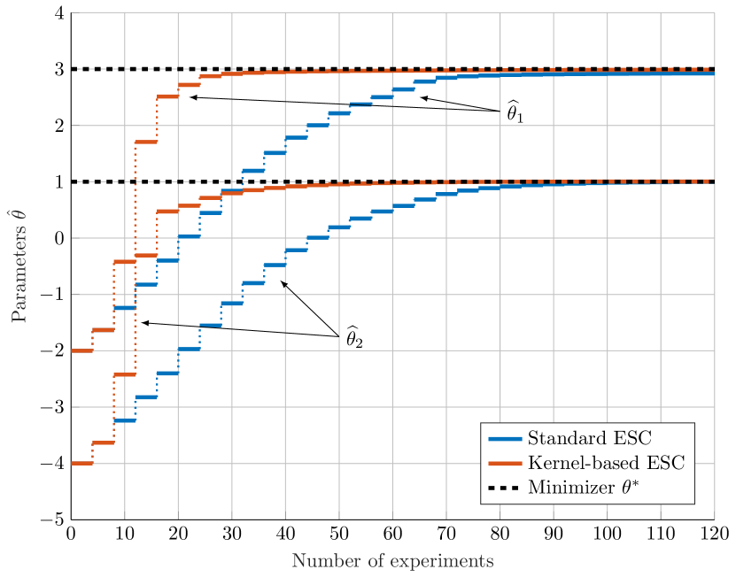
Figure 2: The optimizer state $\widehat{\theta}$ for both ESC approaches as a function of the number of experiments. The proposed kernel-based approach requires only 60 experiments to reach the same neighborhood of the optimum that the standard approach reaches with 100 experiments.

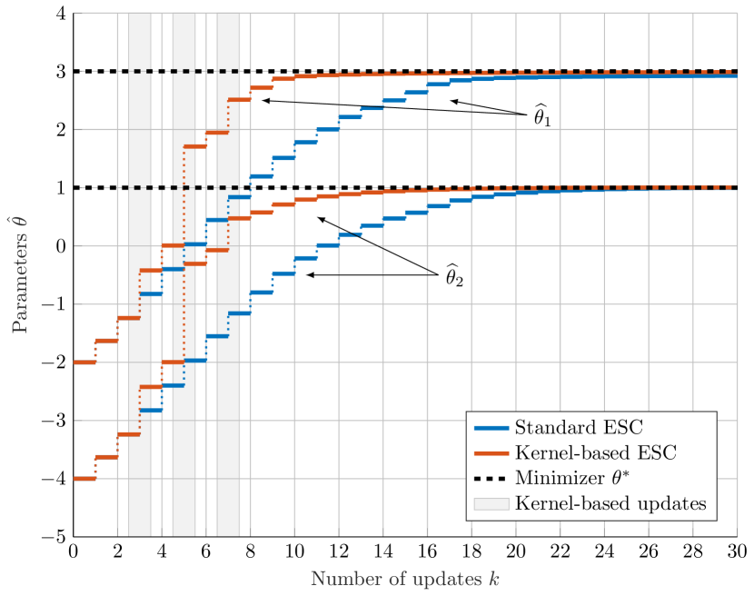
Figure 3: The optimizer state $\widehat{\theta}$ for both ESC approaches as a function of the number of update steps. The third, fifth, and seventh update in the proposed kernel-based approach are kernel-based update steps, which do not require additional experiments to be performed to perform the update and allow searching for a suitable optimizer gain, resulting in needing only 18 update steps to reach the same neighborhood of the optimum as the standard approach does with 25 update steps.

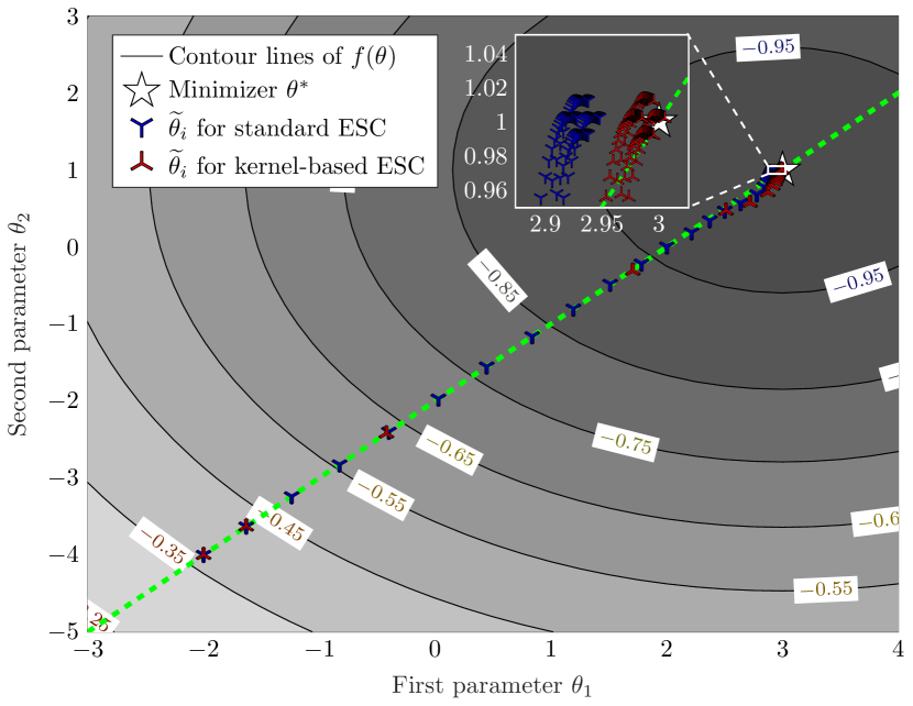
Figure 4: Contour plot of the steady-state input-output map $f(\theta)$, along with inputs $\widetilde{\theta}_{i}$ applied during experiments in both approaches. These applied inputs lie close to the line passing through the initial optimizer state $\widehat{\theta}_{0}$ and the minimizer $\theta^{*}$ (shown in green).

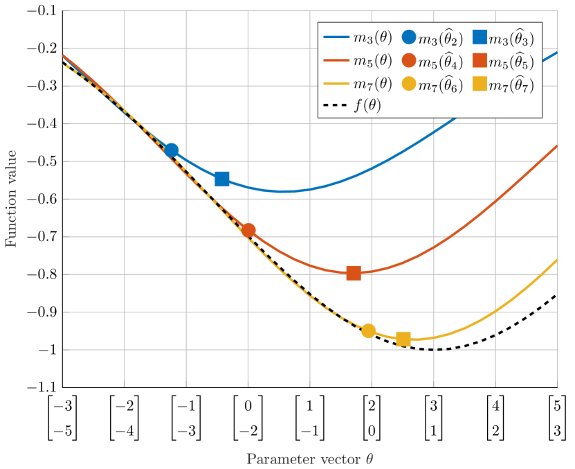
Figure 5: Cross-section of the input-output map $f(\theta)$ as well as the approximation $m_{k}(\theta)$ at different kernel-based update steps, along the search direction (cf. green line in Figure 4). $m_{k}(\theta)$ quickly becomes an accurate approximation of $f(\theta)$ allowing large kernel-based update steps to be taken from the circle to the square.

6 Conclusion

Motivated by the typically slow convergence in extremum-seeking control and the potentially costly nature of performing experiments in practical applications, we presented a novel extremum-seeking approach aimed at increasing the convergence rate and reducing the total number of experiments needed to optimize performance. The proposed approach uses kernel-based function approximation to construct online an approximation of the steady-state input-output map of the system, based on data collected during regular extremum-seeking steps. This approximation is used to determine a suitable search direction and optimizer gain to perform a parameter update without performing additional experiments whenever it is sufficiently accurate to guarantee a decrease in the input-output map. If such decrease cannot be guaranteed, a regular extremum-seeking parameter update step is performed to update the parameters, and the data collected during this update step is used to improve the approximation for the next parameter update step. By using this approach, reductions in both the number of performed experiments and the number of update steps can be obtained, as illustrated by a simulation study in which the number of experiments and updates are reduced by 40% and 28%, respectively.

Future research could consider extensions to a more general class of optimization methods as in Khong et al. (2013a, b), for example, for both the standard parameter update steps and kernel-based update steps. Other potential research directions include the use of variable waiting times instead of a fixed one, as, e.g., in Poveda and Teel (2017), to speed up convergence even further, or extensions in which only a subset of all collected data are used, e.g., to reduce computational complexity or to deal with input-output maps that are slowly changing over time.

Appendix A Proof of Theorem 10

We start the proof by showing that under the conditions in Theorem 10, the bound $\overline{b}(\theta,\mu)$ in (39) is indeed the maximum value that $f(\theta^{+})-f(\theta)+c\mu\nabla f(\theta)^{\intercal}\nabla m_{k}(\theta)$ can obtain given the input $\theta\in\mathbb{R}^{n_{\theta}}$. That is, we will start by showing that (39) is the same as

$$\overline{b}(\theta,\mu)=$$

$$\underset{f\in\mathcal{H}}{\sup} \>f(\theta^{+})-f(\theta)+c\mu\nabla f(\theta)^{\intercal}\nabla m_{k}(\theta)$$ (50a)

s.t. $$\>\lVert f\rVert^{2}\leq\Gamma^{2},$$ (50b)

$$\>\lvert f(\widetilde{\theta}_{i})-\widetilde{y}_{i}\rvert\leq\bar{\delta}\quad\forall i\in\{1,\dots,N_{k}\},$$ (50c)

where $\mathcal{H}$ denotes the reproducing kernel Hilbert space associated with the kernel $\kappa$. The proof follows steps similar to those taken in the proof of Scharnhorst et al. (2023, Theorem 1), i.e., first we show that the search for $f\in\mathcal{H}$ in (50) can be restricted to the finite-dimensional subspace

$$\mathcal{H}^{\parallel}:=\{f\in\; \mathcal{H}:f\in{\rm span}\{\kappa(\cdot,\widetilde{\theta}_{1}),\dots,\kappa(\cdot,\widetilde{\theta}_{N_{k}}),\kappa(\cdot,\theta),$$

$$\kappa(\cdot,\theta^{+}),D^{(0,e_{1})}\kappa(\cdot,\theta),\dots,D^{(0,e_{n_{\theta}})}\kappa(\cdot,\theta)\}\}$$ (51)

with $D^{(0,e_{i})}\kappa(\cdot,\theta)$ as in (32). Next, we show that the supremum in (50) can be replaced by a maximum. Finally, we show that from these two observations it follows that (50) can be written as (39).

Step 1: Note that by the reproducing property of the kernel $\kappa$ and its partial derivatives (Zhou, 2008) we have for any $z\in\mathbb{R}^{n_{\theta}}$ that

$$f(z)=\langle f,\kappa(\cdot,z)\rangle$$ (52)

and

$$\nabla f(z) =\begin{bmatrix}\langle f,D^{(0,e_{1})}\kappa(\cdot,z)\rangle&\dots&\langle f,D^{(0,e_{n_{\theta}})}\kappa(\cdot,z)\rangle\end{bmatrix}^{\intercal}.$$ (53)

Let $\mathcal{H}^{\perp}:=\{g\in\mathcal{H}:\langle g,f^{\parallel}\rangle=0,\,\forall f^{\parallel}\in\mathcal{H}^{\parallel}\}$ be the subspace of functions in $\mathcal{H}$ that are orthogonal to $\mathcal{H}^{\parallel}$ in (51). It then follows that $\mathcal{H}=\mathcal{H}^{\parallel}\oplus\mathcal{H}^{\perp}$, with $\oplus$ denoting the vector direct sum, and that for all $f\in\mathcal{H}$ there exist $f^{\parallel}\in\mathcal{H}^{\parallel}$ and $f^{\perp}\in\mathcal{H}^{\perp}$ such that $f=f^{\parallel}+f^{\perp}$. Using this decomposition of $f$, and observing that $\langle f^{\perp},\kappa(\cdot,z)\rangle$ and $\langle f^{\perp},D^{(0,e_{j})}\kappa(\cdot,\theta)\rangle$ are zero for $z\in\{\widetilde{\theta}_{1},\dots,\widetilde{\theta}_{N_{k}},\theta,\theta^{+}\}$ and $j=1,\dots,n_{\theta}$, respectively, since for those $z$ and $j$ it holds that $\kappa(\cdot,z)\in\mathcal{H}^{\parallel}$, and $D^{{(0,e_{j})}}\kappa(\cdot,\theta)\in\mathcal{H}^{\parallel}$, we obtain using (52) and (53) that (50a) can be written as

$$f(\theta^{+})- f(\theta)+c\mu\nabla f(\theta)^{\intercal}\nabla m_{k}(\theta)$$

$$=f^{\parallel}(\theta^{+})-f^{\parallel}(\theta)+c\mu\nabla f^{\parallel}(\theta)^{\intercal}\nabla m_{k}(\theta)$$ (54)

and that (50c) can be written as

$$\lvert f(\widetilde{\theta}_{i})-\widetilde{y}_{i}\rvert=\lvert f^{\parallel}(\widetilde{\theta}_{i})-\widetilde{y}_{i}\rvert.$$ (55)

Furthermore, it follows from the same decomposition that

$$\lVert f\rVert^{2}=\langle f,f\rangle=\langle f^{\parallel}+f^{\perp},f^{\parallel}+f^{\perp}\rangle=\lVert f^{\parallel}\rVert^{2}+\lVert f^{\perp}\rVert^{2}$$ (56)

since $f^{\parallel}$ and $f^{\perp}$ are orthogonal. Substituting (54)-(56) in (50) we obtain

$$\overline{b}(\theta,\mu)=$$

$$\underset{\begin{subarray}{c}f^{\parallel}\in\mathcal{H}^{\parallel},\\ f^{\perp}\in\mathcal{H}^{\perp}\end{subarray}}{\sup} \>f^{\parallel}(\theta^{+})-f^{\parallel}(\theta)+c\mu\nabla f^{\parallel}(\theta)^{\intercal}\nabla m_{k}(\theta)$$ (57a)

s.t. $$\>\lVert f^{\parallel}\rVert^{2}+\lVert f^{\perp}\rVert^{2}\leq\Gamma^{2},$$ (57b)

$$\>\lvert f^{\parallel}(\widetilde{\theta}_{i})-\widetilde{y}_{i}\rvert\leq\bar{\delta}\quad\forall i\in\{1,\dots,N_{k}\}.$$ (57c)

Note that the objective (57a) does not depend on $f^{\perp}$, and that any $f^{\perp}\neq 0$ would tighten the constraint (57b). Hence, the supremum (if attained) will be attained for $f^{\perp}=0$, and thus the search over $f\in\mathcal{H}$ in (50) can be restricted to the finite-dimensional subspace $\mathcal{H}^{\parallel}$ as in (51).

Step 2: Next, we address the attainment of the supremum by showing that the constraints in (57) define a closed and bounded feasible set. First, note that $\lVert f^{\parallel}\rVert^{2}\leq\Gamma^{2}$ defines a closed and bounded set, since it is the sublevel set of a norm. Next, we note that since sets of the form $\{a\in\mathbb{R}:\lvert a\rvert\leq b\}$ are closed in $\mathbb{R}$, so are $\{f^{\parallel}(\widetilde{\theta}_{i})\in\mathbb{R}:\lvert f^{\parallel}(\widetilde{\theta}_{i})-\widetilde{y}_{i}\rvert\leq\bar{\delta}\}$ $\forall i\in\{1,\dots,N_{k}\}$. Furthermore, the evaluation functional $L_{z}(f^{\parallel})=f^{\parallel}(z)$ is a linear operator and thus the pre-images $L_{z}^{-1}$ of these closed sets are also closed. Consequentially, $\{f^{\parallel}\in\mathcal{H}^{\parallel}:\lvert f^{\parallel}(\widetilde{\theta}_{i})-\widetilde{y}_{i}\rvert\leq\bar{\delta}\}$ $\forall i\in\{1,\dots,N_{k}\}$ are closed in $\mathcal{H}^{\parallel}$. Since the intersection of a finite number of closed sets is necessarily closed, the constraints (57b)-(57c) define a closed feasible set. Moreover, this set is bounded because it is contained in the bounded set defined by the constraint (57b). Since $\mathcal{H}^{\parallel}$ in (51) is finite dimensional, any closed and bounded subset is compact by the Heine-Borel theorem (see, e.g., Royden and Fitzpatrick (2010, Theorem 20)). Therefore, by the extreme value theorem, the continuous objective (57a) attains a maximum on the feasible compact set. Moreover, from Step 1 it follows that the optimizer for which this maximum is obtained must be in $\mathcal{H}^{\parallel}$ ($f^{\perp}=0$), whose members $f^{\parallel}\in\mathcal{H}^{\parallel}$ by (51) have the form

$$f^{\parallel}(\cdot) =\begin{bmatrix}K_{\Omega}(\cdot)&\kappa(\cdot,\theta)&\kappa(\cdot,\theta^{+})&\nabla K(\theta,\cdot)^{\intercal}\end{bmatrix}\beta$$ (58)

with $K_{\Omega}(\cdot)$ as in (29) for the inputs $\Omega=\{\widetilde{\theta}_{1},\dots,\widetilde{\theta}_{N_{k}}\}$, $\nabla K(\theta,\cdot)$ as in (37), and $\beta\in\mathbb{R}^{N_{k}+2+n_{\theta}}$ a weight vector.

Step 3: Finally, we show that it follows from the above that (50) can be written as (39). To this end, note that it follows from the definition of $\mathfrak{K}^{\prime}(\theta,\theta^{+})$ in (36), and (58) and its partial derivatives that

$$\begin{bmatrix}f^{\parallel}(\widetilde{\theta}_{1})&\cdots&f^{\parallel}(\widetilde{\theta}_{N_{k}})&f^{\parallel}(\theta)&f^{\parallel}(\theta^{+})&\nabla f(\theta)^{\intercal}\end{bmatrix}^{\intercal}$$

$$\hphantom{\begin{bmatrix}f^{\parallel}(\widetilde{\theta}_{1})&\cdots&f^{\parallel}(\widetilde{\theta}_{N_{k}})&f^{\parallel}(\theta)\end{bmatrix}^{\intercal}}=\mathfrak{K}^{\prime}(\theta,\theta^{+})\beta$$ (59)

Using (59), the objective (57a) can be written as

$$f^{\parallel} (\theta^{+})-f^{\parallel}(\theta)+c\mu\nabla f^{\parallel}(\theta)^{\intercal}\nabla m_{k}(\theta)$$

$$=\begin{bmatrix}0_{1\times N_{k}}&-1&1&c\mu\nabla m_{k}(\theta)^{\intercal}\end{bmatrix}\mathfrak{K}^{\prime}(\theta,\theta^{+})\beta.$$ (60)

Furthermore, using (58), the definition of $\mathfrak{K}^{\prime}(\theta,\theta^{+})$ in (36), and the reproducing properties (52) and (53), the constraint (57b) can be written similar to (24) as

$$\lVert f^{\parallel}\rVert^{2} =\langle f^{\parallel},f^{\parallel}\rangle=\beta^{\intercal}\mathfrak{K}^{\prime}(\theta,\theta^{+})\beta\leq\Gamma^{2},$$ (61)

while the constraint (57c) can be written as

$$\lvert f^{\parallel}(\widetilde{\theta}_{i})-\widetilde{y}_{i}\rvert=\lvert\xi_{i}^{\intercal}\mathfrak{K}^{\prime}(\theta,\theta^{+})\beta-\widetilde{y}_{i}\rvert\leq\bar{\delta}$$ (62)

for all $i\in\{1,\dots,N_{k}\}$ with $\xi_{i}\in\mathbb{R}^{N_{k}+2+n_{\theta}}$ a vector with $i$-th element equal to one and other elements equal to zero.

Using (60)-(62), and the observation from Step 2 that the objective (57a) attains a maximum on the feasible compact set, we obtain (39) from (57), completing the proof for $\overline{b}(\theta,\mu)$.

The proof that under the conditions in Theorem 10 $\underline{b}(\theta)$ in (38) is a lower bound on $\nabla f(\theta)^{\intercal}\nabla m_{k}(\theta)$, i.e., that (38) is the same as

$$\underline{b}(\theta)=$$

$$\underset{f\in\mathcal{H}}{\inf}\> \nabla f(\theta)^{\intercal}\nabla m_{k}(\theta)$$ (63a)

s.t. $$\lVert f\rVert^{2}\leq\Gamma^{2},$$ (63b)

$$\lvert f(\widetilde{\theta}_{i})-\widetilde{y}_{i}\rvert\leq\bar{\delta}\quad\forall i\in\{1,\dots,N_{k}\},$$ (63c)

follows mutatis mutandis from the above proof by omitting $\kappa(\cdot,\theta)$ and $\kappa(\cdot,\theta^{+})$ from the span in (51), using $\mathfrak{K}(\theta)$ as in (34) instead of $\mathfrak{K}^{\prime}(\theta,\theta^{+})$ as in (36), removing $f(\theta^{+})$, $f(\theta)$, $c$, and $\mu$ from the objective (50a), and taking the infimum instead of the supremum.

Appendix B Proof of Lemma 13

The proof of Lemma 13 is as follows. Since by the conditions of the lemma $\overline{b}(\theta,\mu)\leq 0$, it follows from Theorem 10 that the inequality $f(\theta^{+})\leq f(\theta)-c\mu\nabla f(\theta)^{\intercal}\nabla m_{k}(\theta)$ with $c\in(0,1)$ is satisfied. Therefore, using the definitions of $V(\cdot)$ and $\Delta V(\cdot)$ in (40) and (44), we obtain that the inequality

$$\Delta V(\theta) =f(\theta^{+})-f(\theta)\leq-c\mu\nabla f(\theta)^{\intercal}\nabla m_{k}(\theta)$$ (64)

holds. Furthermore, since by the conditions of the lemma $\underline{b}(\theta)>0$ for all $\theta\in\mathbb{R}\backslash\mathcal{C}$, and by Assumption 2(iii) $\nabla f(\theta)=0$ if and only if $\theta\in\mathcal{C}$, it follows from Theorem 10 and (64) that $\Delta V(\theta)<0$ for all $\theta\in\mathbb{R}^{n_{\theta}}\backslash\mathcal{C}$ and $\Delta V(\theta)=0$ for all $\theta\in\mathcal{C}$. Hence, for any $\Delta_{\theta}$ such that $\lVert\theta\rVert_{\mathcal{C}}\leq\Delta_{\theta}$, there exists a class-$\mathcal{K}$ function $\bar{\rho}_{k}$ such that $\bar{\rho}_{k}(\lVert\theta\rVert_{\mathcal{C}})\leq-\Delta V(\theta)$ (see, e.g., Khalil (2002, Lemma 4.3)). Moreover, it follows from the definition of $V(\cdot)$ in (40) and Assumption 10 that $\lVert\theta\rVert_{\mathcal{C}}\geq\omega_{2}^{-1}(V(\theta))$ and thus that $-\bar{\rho}_{k}(\lVert\theta\rVert_{\mathcal{C}})\leq-\bar{\rho}_{k}(\omega_{2}^{-1}(V(\theta)))$. Therefore, we obtain from (64) that during kernel-based extremum-seeking steps the inequality

$$\Delta V(\theta)\leq-\bar{\rho}_{k}(\lVert\theta\rVert_{\mathcal{C}})\leq-\widetilde{\rho}_{k}(V(\theta)),$$ (65)

with $\widetilde{\rho}_{k}:=\bar{\rho}_{k}(\omega_{2}^{-1}(\cdot))$ a function of class $\mathcal{K}$, holds for all $\theta$ such that $\lVert\theta\rVert_{\mathcal{C}}\leq\Delta_{\theta}$, which completes the proof.

Appendix C Proof of Theorem 15

The proof of Theorem 15 consists of three steps. In the first two steps of the proof the increments of Lemmas 12 and 13 are used to derive upper bounds on $W(\psi,x,\theta)$ after a sequence of, respectively, standard or kernel-based update steps. In the third step of the proof, these upper bounds are combined to determine an upper bound that holds for either type of update step, from which it can be concluded that $\lVert\theta\rVert_{\mathcal{C}}$ ultimately converges to the level set of $\lVert\cdot\rVert_{\mathcal{C}}$ given in the theorem.

Step 1: We first show that from Lemma 12 it follows that $W(\psi,x,\theta)$ is upper bounded during standard update steps by the maximum of a class-$\mathcal{K}\mathcal{L}$ function and a constant. To this end, let $\widehat{\rho}$ be a class-$\mathcal{K}_{\infty}$ function such that $({\rm id}-\widehat{\rho})\in\mathcal{K}_{\infty}$. By Lemma 12, it then follows that for any $\theta,\psi\in\mathbb{R}^{n_{\theta}}$ and $x\in\mathcal{X}$ such that $\lVert\theta\rVert_{\mathcal{C}}\leq\Delta_{\theta}$, $\lVert\psi\rVert_{\mathcal{C}}\leq\Delta_{\theta}$, and $\lVert x\rVert_{\mathcal{A}(\psi+v_{n_{v}}(\theta))}\leq\Delta_{x}$, the inequality

$$\Delta W(\psi,x,\theta) \leq-\widetilde{\gamma}\left(W(\psi,x,\theta)\right)+\gamma+2\delta+\delta_{V}$$ (66)

$$=-({\rm id}-\widehat{\rho})\circ\widetilde{\gamma}\left(W(\psi,x,\theta)\right)+\gamma+2\delta$$

$$\hphantom{=~}+\delta_{V}-\widehat{\rho}\circ\widetilde{\gamma}\left(W(\psi,x,\theta)\right)$$ (67)

$$\leq-({\rm id}-\widehat{\rho})\circ\widetilde{\gamma}\left(W(\psi,x,\theta)\right)$$ (68)

holds as long as $\widehat{\rho}\circ\widetilde{\gamma}(W(\psi,x,\theta))\geq\gamma+2\delta+\delta_{V}$. From (68) and the comparison lemma (see, e.g., Jiang and Wang (2002, Lemma 4.3)), it follows that there exists a class-$\mathcal{K}\mathcal{L}$ function $\beta_{1}$ such that

$$W(\psi_{k+\ell},x_{k+\ell},\theta_{k+\ell})\leq\max\{ \beta_{1}(W(\psi_{k},x_{k},\theta_{k}),\ell),$$

$$\;\varphi(\gamma+2\delta+\delta_{V})\}$$ (69)

for a sequence of $\ell$ standard update steps starting at any update number $k$, with $\varphi(\cdot):=\widetilde{\gamma}^{-1}\circ\widehat{\rho}^{-1}(\cdot)$ a function of class $\mathcal{K}_{\infty}$.

Step 2: Next, note that a kernel-based update (20) is only performed if $\underline{b}(\theta)>0$ and with $\mu\in\mathbb{R}_{>0}$ chosen such that $\overline{b}(\theta,\mu)\leq 0$ (cf. Algorithm 2). Therefore, it follows from Lemma 13 that

$$\Delta V(\theta)\leq-\widetilde{\rho}_{k}(V(\theta))$$ (70)

for any $\theta\in\mathbb{R}^{n_{\theta}}$ such that $\lVert\theta\rVert_{\mathcal{C}}\leq\Delta_{\theta}$ at any kernel-based update step $k$. Therefore, for a sequence of $\ell$ kernel-based update steps, starting at update step $k$, it holds that

$$\Delta V(\theta)\leq-\underline{\rho}_{k,\ell}(V(\theta))$$ (71)

at every step, where $\underline{\rho}_{k,\ell}(\cdot):=\min\{\widetilde{\rho}_{k}(\cdot),\dots,\widetilde{\rho}_{k+\ell}(\cdot)\}$ is a function of class $\mathcal{K}$. Similar to Step 1, we conclude from (71) and the comparison lemma that there exists a class-$\mathcal{K}\mathcal{L}$ function $\beta_{2}$ such that

$$V(\theta_{k+\ell})\leq\beta_{2}(V(\theta_{k}),\ell)$$ (72)

for a sequence of $\ell$ kernel-based update steps starting at any update number $k$. Substituting (72) in the definition of $W(\psi,x,\theta)$ in (41), we obtain that

$$W (\psi_{k+\ell},x_{k+\ell},\theta_{k+\ell})\leq V_{p}(\psi_{k+\ell},x_{k+\ell})+2\beta_{2}(V(\theta_{k}),\ell)$$ (73)

during a sequence of $\ell$ kernel-based update steps starting from update number $k$. Note that during this sequence, the memory state $\psi$ and the system state $x$ do not change, since the input applied to the system $\Sigma_{p}$ is not changed during kernel-based update steps (cf. Algorithm 2, Line 17), and since kernel-based update steps are instantaneous (because there is no waiting time $T$ for these steps).

Step 3: Finally, we combine the observations from Steps 1 and 2 to draw conclusions about the level set of $\lVert\cdot\rVert_{\mathcal{C}}$ to which $\lVert\theta\rVert_{\mathcal{C}}$ converges. To this end, note that it follows from (69) and (73) that

$$W( \psi_{k+\ell},x_{k+\ell},\theta_{k+\ell})$$

$$\leq\max\{\beta_{1}(W(\psi_{k},x_{k},\theta_{k}),\ell),\,\varphi(\gamma+2\delta+\delta_{V}),$$

$$\hphantom{\leq~\max\{}\;V_{p}(\psi_{k+\ell},x_{k+\ell})+2\beta_{2}(V(\theta_{k}),\ell)\}$$ (74)

for a sequence of $\ell$ update steps of either type starting from update number $k$. Subtracting $V_{p}(\psi_{k+\ell},x_{k+\ell})$ from both sides in (74) and noting that $V_{p}(\psi,x)\geq 0$, it thus follows using the definition of $W(\psi,x,\theta)$ in (41) that

$$2V(\theta_{k+\ell})\leq\max\{ \beta_{1}(W(\psi_{k},x_{k},\theta_{k}),\ell),\,2\beta_{2}(V(\theta_{k}),\ell),$$

$$\;\varphi(\gamma+2\delta+\delta_{V})\}.$$ (75)

Since both $\beta_{1}$ and $\beta_{2}$ are functions of class $\mathcal{K}\mathcal{L}$, it follows from (75) that starting from the initial update $k=0$, $V(\theta)$ is ultimately bounded by

$$\lim_{\ell\to\infty}V(\theta_{\ell})\leq\frac{1}{2}\varphi(\gamma+2\delta+\delta_{V}).$$ (76)

Finally, since $\omega_{1}(\lVert\theta\rVert_{\mathcal{C}})\leq V(\theta)$ by Assumption 10 and the definition of $V(\cdot)$ in (40), we obtain from (76) that the optimizer state $\theta$ ultimately converges to the set

$$\left\{\theta\in\mathbb{R}^{n_{\theta}}:\lVert\theta\rVert_{\mathcal{C}}\leq\omega_{1}^{-1}\left(\frac{1}{2}\varphi(\gamma+2\delta+\delta_{V})\right)\right\}.$$ (77)

Since $\gamma$, $\delta$, and $\delta_{V}$ can be made arbitrarily small by Lemma 12, this set to which $\theta$ converges can be made arbitrarily small, completing the proof.

References

- Aronszajn (1950) Aronszajn, N., 1950. Theory of reproducing kernels. Transactions of the American Mathematical Society 68, 337–404.
- Gelbert et al. (2012) Gelbert, G., Moeck, J.P., Paschereit, C.O., King, R., 2012. Advanced algorithms for gradient estimation in one- and two-parameter extremum seeking controllers. Journal of Process Control 22, 700–709.
- Guay and Dochain (2015) Guay, M., Dochain, D., 2015. A time-varying extremum-seeking control approach. Automatica 51, 356–363.
- Haring and Johansen (2018) Haring, M.A.M., Johansen, T.A., 2018. On the accuracy of gradient estimation in extremum-seeking control using small perturbations. Automatica 95, 23–32.
- Hazeleger et al. (2022) Hazeleger, L., Nešić, D., Van de Wouw, N., 2022. Sampled-data extremum-seeking framework for constrained optimization of nonlinear dynamical systems. Automatica 142, 110415.
- Hunnekens et al. (2014) Hunnekens, B.G.B., Haring, M.A.M., Van de Wouw, N., Nijmeijer, H., 2014. A dither-free extremum-seeking control approach using 1st-order least-squares fits for gradient estimation, in: 53rd IEEE Conference on Decision and Control, IEEE. pp. 2679–2684.
- Jiang and Wang (2002) Jiang, Z.P., Wang, Y., 2002. A converse Lyapunov theorem for discrete-time systems with disturbances. Systems & Control Letters 45, 49–58.
- Khalil (2002) Khalil, H.K., 2002. Nonlinear Systems. Third ed., Prentice Hall.
- Khong et al. (2013a) Khong, S.Z., Nešić, D., Manzie, C., Tan, Y., 2013a. Multidimensional global extremum seeking via the DIRECT optimisation algorithm. Automatica 49, 1970–1978.
- Khong et al. (2013b) Khong, S.Z., Nešić, D., Tan, Y., Manzie, C., 2013b. Unified frameworks for sampled-data extremum seeking control: Global optimisation and multi-unit systems. Automatica 49, 2720–2733.
- Krstić and Wang (2000) Krstić, M., Wang, H.H., 2000. Stability of extremum seeking feedback for general nonlinear dynamic systems. Automatica 36, 595–601.
- Kvaternik and Pavel (2011) Kvaternik, K., Pavel, L., 2011. Interconnection conditions for the stability of nonlinear sampled-data extremum seeking schemes, in: IEEE Conference on Decision and Control and European Control Conference, IEEE. pp. 4448–4454.
- Micchelli et al. (2006) Micchelli, C.A., Xu, Y., Zhang, H., 2006. Universal kernels. Journal of Machine Learning Research 7, 2651–2667.
- Nocedal and Wright (2006) Nocedal, J., Wright, S.J., 2006. Numerical Optimization. Second ed., Springer New York.
- Poveda et al. (2021) Poveda, J.I., Benosman, M., Vamvoudakis, K.G., 2021. Data‐enabled extremum seeking: A cooperative concurrent learning‐based approach. International Journal of Adaptive Control and Signal Processing 35, 1256–1284.
- Poveda and Teel (2017) Poveda, J.I., Teel, A.R., 2017. A robust event-triggered approach for fast sampled-data extremization and learning. IEEE Transactions on Automatic Control 62, 4949–4964.
- Rodrigues et al. (2022) Rodrigues, V.H.P., Hsu, L., Oliveira, T.R., Diagne, M., 2022. Event-triggered extremum seeking control. IFAC PapersOnLine 55, 555–560.
- Rodrigues et al. (2023) Rodrigues, V.H.P., Hsu, L., Oliveira, T.R., Diagne, M., 2023. Dynamic event-triggered extremum seeking feedback. IFAC PapersOnLine 56, 10307–10314.
- Royden and Fitzpatrick (2010) Royden, H.L., Fitzpatrick, P.M., 2010. Real Analysis. Fourth ed., Pearson.
- Ryan and Speyer (2010) Ryan, J.J., Speyer, J.L., 2010. Peak-seeking control using gradient and Hessian estimates, in: Proceedings of the 2010 American Control Conference, IEEE. pp. 611–616.
- Scharnhorst et al. (2023) Scharnhorst, P., Maddalena, E.T., Jiang, Y., Jones, C.N., 2023. Robust uncertainty bounds in reproducing kernel Hilbert spaces: A convex optimization approach. IEEE Transactions on Automatic Control 68, 2848–2861.
- Scheinker (2024) Scheinker, A., 2024. 100 years of extremum seeking: A survey. Automatica 161.
- Schölkopf et al. (2001) Schölkopf, B., Herbrich, R., Smola, A.J., 2001. A generalized representer theorem, in: Helmbold, D., Williamson, B. (Eds.), Computational Learning Theory, Springer Berlin Heidelberg. pp. 416–426.
- Tan et al. (2010) Tan, Y., Moase, W.H., Manzie, C., Nešić, D., Mareels, I.M.Y., 2010. Extremum seeking from 1922 to 2010, in: Proceedings of the 29th Chinese Control Conference, IEEE. pp. 14–26.
- Tan et al. (2006) Tan, Y., Nešić, D., Mareels, I.M.Y., 2006. On non-local stability properties of extremum seeking control. Automatica 42, 889–903.
- Teel and Popović (2001) Teel, A.R., Popović, D., 2001. Solving smooth and nonsmooth multivariable extremum seeking problems by the methods of nonlinear programming, in: Proceedings of the 2001 American Control Conference, IEEE. pp. 2394–2399.
- Van Keulen et al. (2020) Van Keulen, T., Van der Weijst, R., Oomen, T., 2020. Fast extremum seeking using multisine dither and online complex curve fitting. IFAC PapersOnLine 53, 5362–5367.
- Weekers et al. (2023) Weekers, W., Saccon, A., Van de Wouw, N., 2023. Data-efficient static cost optimization via extremum-seeking control with kernel-based function approximation, in: 62nd IEEE Conference on Decision and Control (CDC), pp. 6761–6767.
- Zhou (2008) Zhou, D.X., 2008. Derivative reproducing properties for kernel methods in learning theory. Journal of Computational and Applied Mathematics 220, 456–463.