Enhanced Dissipation via Time-Dependent Velocity Fields: Acceleration and Intermittency

Abstract

Motivated by mixing processes in analytical laboratories, this work investigates enhanced dissipation in non-autonomous flows. Specifically, we study the evolution of concentrations governed by the advection-diffusion equation, where the velocity field is modelled as the product of a shear flow (with simple critical points) and a time-dependent function $\xi(t)$. The main objective of this paper is to derive explicit, quantitative estimates for the energy decay rates, which are shown to depend sensitively on the properties of $\xi$.

We identify a class of time-dependent functions $\xi$ that are bounded above and below by increasing functions of time. For this class, we demonstrate super-enhanced dissipation, characterized by energy decay rates faster than those observed in autonomous cases (e.g., when $\xi\equiv 1$, as in Coti Zelati and Gallay (2023)).

Additionally, we explore enhanced dissipation in the context of intermittent flows, where the velocity fields may be switched on and off over time. In these cases, the dissipation rates are comparable to those of autonomous flows but with modified constants. To illustrate our results, we analyse two prototypical intermittent flows: one that exhibits a gradual turn-on and turn-off phase, and another that undergoes a significant acceleration following a slow initial activation phase. For the second, we derive the corresponding dissipation rate using a ”gluing” argument.

Both results are achieved through the application of the “hypocoercivity” framework (à la Bedrossian and Coti Zelati (2017)), adapted to an augmented functional with time-dependent weights. These weights are designed to dynamically counteract the potential growth of $\xi$, ensuring robust estimates for the energy decay.

[Surrey]organization=School of Mathematics and Physics, University of Surrey,city=Guildford, postcode=GU2 7XH, country=UK

1 Introduction

On the set $\Omega=\mathbb{T}^{2}\times[0,\infty)$, let the concentration $\Theta=\Theta(x,y,t):\Omega\rightarrow\mathbb{R}$, and velocity field $\bm{u}=\bm{u}(x,y,t):\Omega\rightarrow\mathbb{R}^{2}$ solve the Cauchy problem for the advection-diffusion equation

$$\begin{array}[]{rrl}\partial_{t}\Theta+\bm{u}\cdot\nabla\Theta-\nu\Delta\Theta&=&0\\ \nabla\cdot\bm{u}&=&0\\ \Theta(x,y,0)&=&\Theta_{0}(x,y,t)\,,\end{array}$$ (1.1)

where $\nu\ll 1$ is the molecular diffusivity. Further, we consider the special class of time-dependent shear flows of the type

$$\bm{u}(x,y,t)=(v(y,t),0)^{T},$$ (1.2)

for which the advection-diffusion equation reduces to

$$\partial_{t}\hat{\Theta}+v(y,t)ik\hat{\Theta}=\nu(-k^{2}+\partial_{y}^{2})\hat{\Theta}\,.$$ (1.3)

where we conveniently Fourier transformed in the $x$-variable. In this work, we are interested in demonstrating enhanced dissipation under specific assumptions on the time-dependent velocity fields. Enhanced dissipation is a physical phenomenon intrinsically connected with mixing [1]. Mixing generates gradients, i.e. high frequencies, and its effect for inviscid fluids has been widely studied (see the excellent survey [2] and references therein). For viscous fluids, diffusion acts to smooth out irregularities, effectively damping high-frequency components. The interplay between advection and diffusion leads to intricate physical phenomena [3, 4, 5], including the phenomenon known as enhanced dissipation. Although physically well understood, its mathematical characterization has only recently been explored in specific settings due to its inherent complexity. In their seminal paper [6], Constantin et al. characterize flows that induce enhanced dissipation, in terms of the spectral properties of the dynamical system associated with it. In [7] the authors quantify the enhanced dissipation effect due to shear by employing the hypocoercivity method introduced by Villani [8]. In particular, assumptions on the form of the shear are made, and the rates depend significantly on the maximal order of degeneracy of the flow’s critical points. As already mentioned, enhanced dissipation and mixing are connected phenomena: the authors in [9] establish a precise connection between quantitative mixing rates in terms of decay of negative Sobolev norms and enhanced dissipation time-scales. Mixing with diffusion is also at the base of the Batchelor scale conjecture, as stated by Charlie Doering in [3]. This conjecture asserts that the filamentation length, defined as the ratio of the $H^{-1}$-norm to the $L^{2}$-norm of the scalar concentration, converges to a constant known as the Batchelor scale in the long-time limit. This provides an equivalent formulation, from a PDE perspective, of the theory of strange eigenmodes [4], which is rooted in a dynamical systems approach. In [10] the authors study the long time asymptotics of the filamentation length in the whole space, where they could make use of Fourier splitting technique. To the authors’ knowledge, the study of long time asymptotics of the filamentation length on bounded domains remains an open problem.

For autonomous shear flows, enhanced dissipation is well-established in the literature, and we therefore point towards [11] for reference. There the authors, inspired by [7], establish enhanced dissipation in the infinite channel $\mathbb{R}\times[0,1]$, assuming that $\Theta$ satisfies Neumann boundary conditions and the velocity profile $v(y)$ is either monotonic or has only finitely many simple critical points. These critical points, denoted $\{y_{i}\}_{i=1}^{N}$, satisfy

$$v^{\prime\prime}(y_{j})\neq 0\quad\text{for }j=1,\dots,N.$$ (1.4)

Under these conditions, they prove

$$\|\hat{\Theta}(t)\|_{L^{2}}\leq C_{1}\exp(-C_{2}\lambda_{\nu,k}t-\nu k^{2}t)\|\hat{\Theta}_{0}\|_{L^{2}}\qquad\mbox{ for all }t\geq 0$$ (1.5)

with

$$\lambda_{\nu,k}=\begin{cases}\nu^{\frac{m}{m+2}}|k|^{\frac{2}{m+2}}&\text{if }0<\nu<|k|,\\[6.0pt] \frac{k^{2}}{\nu}&\text{if }0<|k|<\nu.\end{cases}$$

Notably, the authors demonstrate that this result can be equivalently derived using both a spectral approach (à la Wei [12]) and the hypocoercivity method. The above rate is sharp for time-independent flows, as proven in [13]. Hence, the above decay estimate for the case of $m=2$ will be our main point of reference when referring to the autonomous setting.

In $2D$, a generalization of this result to the case where $v$ admits a finite number of possibly degenerate critical points, as well as to geometries like the torus $\mathbb{T}^{2}$ and the periodic channel $\mathbb{T}\times[0,1]$, can be found in the aforementioned seminal work [7].

In contrast, the case of a time-dependent velocity field, although physically relevant, has been explored far less in the mathematics literature. Our interest in this scenario is motivated by practical applications. In analytical laboratories, cell disruption is commonly achieved using vortex mixers, which generate violent, high-speed vortexing action. Starting from a state of rest, these mixers rapidly accelerate to very high speeds; this allows for fine adjustments in the mixing intensity, ranging from gentle agitation to vigorous vortexing. Just as crucial is the controlled deceleration of the mixer back to zero, ensuring that sensitive structures are not damaged during the slowdown phase. In chemical and analytical laboratories, a wide variety of stirring devices are employed, each carefully designed to achieve optimal mixing by generating a strongly time-dependent stirring field.

Motivated by these considerations, in this paper we aim at quantifying the effect of time dependent velocity fields in enhanced dissipation estimates. One major challenge in the mathematical analysis of such flows stems from the limitations of the hypocoercivity method when applied to general time-dependent velocity fields, as we will elaborate in the following discussion.
To this end, we consider velocity fields for which the $v(y,t)$ part separates into a space-time product of the form

$$v(y,t)=\xi(t)v(y),\quad\text{with }\xi(t)\geq 0,$$ (1.6)

reducing equation (1.3) to

$$\partial_{t}\hat{\Theta}+\xi(t)v(y)ik\hat{\Theta}=\nu(-k^{2}+\partial_{y}^{2})\hat{\Theta}.$$ (1.7)

This class of velocity fields for the case of $\xi(t)$ being a piecewise constant random function was already considered in [14]. In order to study the decay rate of $\|\Theta(t)\|_{L^{2}}$ in the regime where advection dominates diffusion, i.e. small viscosities, the author performs a boundary-layer analysis effectively reducing the problem to the study of a pair of coupled stochastic differential equations independent of diffusivity. In this paper, we will consider only deterministic functions $\xi(t)$ in $L^{2}([0,T])$ and shear velocities $v\in H^{1}_{y}(\mathbb{T})$, for which well posedness holds [15] (see also [16]).

In order to illustrate how the time-dependent function $\xi(t)$ affects the decay rates of the scalar concentration, we first consider the inviscid case $\nu=0$. Applying the method of stationary phases [17], it is easy to show the upper bound

$$\norm{\hat{\Theta}(k,y,t)}_{H^{-1}}\leq\min\left\{\frac{C_{m}}{\absolutevalue{k}\Xi(t)},1\right\}\norm{\hat{\Theta}_{0}(k,y)}_{H^{1}}\,,$$

where $\Xi(t)=\int_{0}^{t}\xi(\tau)\,d\tau\,$ (see proof in Appendix A). This coincides with the mixing estimate in [9] when $\xi=1$.

We observe that, if $\xi(t)$ increases sufficiently quickly (for instance, if $\xi(t)\gtrsim\alpha t^{\alpha-1}$ for some $\alpha>1$ and all $t\leq T$), the upper bound indicates that the mixing is enhanced over long times compared to the autonomous scenario. If $\xi(t)$ is bounded from below and above by constants, then the result in [9] immediately provides an enhanced dissipation estimate for the advection diffusion equation (see discussion in Appendix A).

Recently, in some particular settings, time dependent velocity fields have been investigated in relation to their dissipation enhancing properties. In [18], the authors investigate the two-dimensional linearized Navier-Stokes equations around the Kolmogorov flow, defined as

$$V_{\rm{NS}}=\big{(}-ae^{-\nu t}\cos y,0\big{)}^{T}.$$

By neglecting the non-local component of the linearized operator

$$\mathcal{L}_{\nu}=-\nu\Delta-ae^{-\nu t}\cos y\partial_{x}(1+\Delta^{-1}),$$

they focus on the vorticity equation

$$\partial_{t}\omega-\nu\Delta\omega-ae^{-\nu t}\cos y\partial_{x}\omega=0.$$

Using the hypocoercivity method, they establish the enhanced dissipation estimate

$$\|\omega(t)\|_{X}\lesssim e^{-c\sqrt{\nu}t}\|\omega_{0}\|_{X},$$ (1.8)

where $X\subset L^{2}$ is a Banach space (see [18, Theorem 3.2]).

In [19], the authors revisited the non-local component of the linearized operator and established (1.8) with $X=L^{2}(\mathbb{T}^{2}_{\delta})$ where $\mathbb{T}^{2}_{\delta}=\{(x,y):0<x<2\pi\delta,\,0<y<2\pi\}$ with $\delta<1$.

Velocities of the form $e^{-\nu t}v(y)$, where $v\in C^{2}$, also belong to the class analysed in [20]. There the authors obtain an extension of [7] in the sense that they recover the classical result of (1.5) $(m=1,2)$ for certain time-dependent flows. We also note the insightful work in [21], where the author, using optimal transport techniques, provides upper bounds on the exponential rates of enhanced dissipation for a broad class of velocity fields without imposing specific structural assumptions, relying only on regularity conditions such as $\int_{0}^{t}\|\nabla\mathbf{u}\|_{L^{p}}\lesssim 1+t^{\alpha}.$

A central and novel aspect of our work lies in the derivation of time-sensitive estimates that precisely capture the evolution of the non-autonomous flow, avoiding bounding $\xi(t)$ by a constant in key steps. In order to achieve this, we embed the flow’s dynamics directly into the hypocoercivity framework. For the targeted class of flows, the proof of our first result leverages time-dependent weights that are dynamically linked to $\xi(t)$, while in our second result we introduce it directly into the functional.

Our first result is an enhanced dissipation estimate for a specific class of velocity fields for which the time-dependent part satisfies polynomial lower and upper bounds.

Theorem 1.

Let $\nu\ll 1$ and $\hat{\Theta}$ be a solution of (1.7) with $\hat{\Theta}_{0}$ in $L^{2}(\mathbb{T})$. Suppose that $v:\mathbb{T}\rightarrow\mathbb{R}$ is a $C^{2}$ function admitting only a finite number of simple critical points (i.e. satisfying (1.4)). Define the weights $w_{\nu}(t):=(1+\nu^{s}t)^{-1}$ for some $s\in[0,\infty)$. Let $\beta\in[\frac{\nu}{|k|},1]$ and assume that $\xi(t)$ satisfies

$$L(t)\leq\xi(t)\leq U(t)\qquad\forall t\in[0,T]\,,$$ (1.9)

where

$$\begin{array}[]{rl}L(t)&=\begin{cases}C^{2}\beta^{2}&\text{for }t\leq t^{*}_{\nu,k}\\ \frac{\nu}{|k|\beta}w_{\nu}(t)^{-2}&\text{for }t\geq t^{*}_{\nu,k}\end{cases}\\[8.0pt] &\quad\text{where}\quad t^{\ast}_{\nu,k}=\frac{1}{\nu^{s}}\left(\frac{|k|^{\frac{1}{2}}C\beta^{\frac{3}{2}}}{\nu^{\frac{1}{2}}}-1\right),\\[15.0pt] U(t)&=w_{\nu}(t)^{-\ell}\quad\text{for some }\ell\in[2,4],\end{array}$$

where $C$ is some positive constant. Then the $L^{2}$ decay estimate

$$\|\hat{\Theta}(t)\|_{L^{2}}^{2}\leq C_{\rm{ed}}\quantity(1+\quantity(\frac{\absolutevalue{k}}{\nu})^{1/2})\exp\left(-\frac{1}{4}(\beta\nu\absolutevalue{k})^{\frac{1}{2}}\int_{0}^{t}\xi(\tau)^{\frac{1}{2}}w_{\nu}(\tau)\,d\tau-\nu k^{2}t\right)\norm{\hat{\Theta}_{0}}_{L^{2}}^{2}$$ (1.10)

holds for any $t\leq T$ where the time $T$ is arbitrary but finite and $C_{\rm{ed}}$ is some constant independent of $\nu,k$.

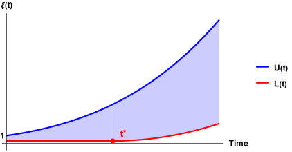
Figure 1: Illustrative sketch of the upper and lower bounds for $\xi(t)$ in Theorem 1. The shaded area is the admissible region for $\xi(t)$.

We observe that when $w_{\nu}=1$ (formally corresponding to $s\rightarrow\infty$), for $\xi(t)$ satisfying

$$C^{2}\beta^{2}\leq\xi(t)\leq 1\qquad\forall t\in[0,T]\,,$$ (1.11)

the result in Theorem 1 reads

$$\|\hat{\Theta}(t)\|_{L^{2}}^{2}\leq C_{\rm{ed}}\quantity(1+\quantity(\frac{\absolutevalue{k}}{\nu})^{1/2})\exp\left(-\frac{1}{4}(\beta^{2}\nu\absolutevalue{k})^{\frac{1}{2}}\int_{0}^{t}\xi(\tau)^{\frac{1}{2}}\,d\tau-\nu k^{2}t\right)\norm{\hat{\Theta}_{0}}_{L^{2}}^{2}.$$ (1.12)

Note that the prefactor $1+\quantity(\frac{\absolutevalue{k}}{\nu})^{1/2}$ in the above decay estimates represents a logarithmic correction and is of purely technical origin (as observed in [7, 22]), but might be removed by the employment of time-dependent weights as in [19].

The bound in (1.12) holds for $\xi=1$, corresponding to the class of time-independent velocities considered in [11, 7]. As mentioned above, the function $\xi(t)=e^{-\nu t}$ was already considered in [18, 19, 20]. Note that, if we fix the maximal time to be the purely diffusive timescale $T=\frac{1}{\nu}$ (we are not interested in later times anyhow) then $\xi(t)=e^{-\nu t}$ satisfies the bounds in (1.11) with the lower bound given by the constant $e^{-1}$. Bounded oscillatory functions such as $\xi(t)=\frac{1}{4}\cos(t)+\frac{1}{2}$ are also admissible in the class (1.11). For all these functions, bounded from above and below by constants as in (1.11), our estimate indicates enhanced dissipation with a rate comparable in scaling to $e^{c(|k|\nu)^{\frac{1}{2}}t}$. Our result in Theorem 1 however goes beyond this class, allowing growth of the velocity in time, yielding a rate that is actually faster than $e^{c(|k|\nu)^{\frac{1}{2}}t}$. We will illustrate such a super enhanced dissipation phenomena with an example. Fix $s=\frac{1}{4}$ and consider

$$\xi(t)=(1+\nu^{1/4}t)^{4}\,,$$ (1.13)

corresponding to the fastest growth allowed from the upper bound in (1.9). The integral in the decay rate can be computed explicitly as

$$\int_{0}^{t}\xi(\tau)^{\frac{1}{2}}w_{\nu}(\tau)\,d\tau=\int_{0}^{t}(1+\nu^{1/4}\tau)\,d\tau=t+\frac{\nu^{1/4}}{2}t^{2}.$$

yielding the exponential decay $e^{-\bar{c}(\nu\absolutevalue{k})^{1/2}\quantity(\frac{\nu^{1/4}}{2}t^{2}+t)}$, which is clearly faster than $e^{-\bar{c}(\nu\absolutevalue{k})^{1/2}t)}$. To see this, recall that, on the one hand, at the enhanced dissipation time $t_{\rm{ed}}=\frac{1}{\nu^{1/2}}$ the time-independent velocity field considered in [11] (and all the velocities of the type $\xi(t)v(y)$ where $\xi(t)$ is the class (1.11)) produces a factor $\sim e^{-\absolutevalue{k}^{1/2}}$. On the other hand, for the velocity field defined by (1.13), at time $t_{\rm{ed}}=\frac{1}{\nu^{1/2}}$ we have

$$\int_{0}^{t_{ed}}(1+\nu^{1/4}\tau)\,d\tau=\frac{1}{2}\frac{1}{\nu^{3/4}}+\frac{1}{\nu^{1/2}}\Rightarrow\|\hat{\Theta}(t_{\rm{ed}})\|_{L^{2}}^{2}\lesssim e^{-\frac{\absolutevalue{k}^{1/2}}{\nu^{1/4}}}.$$

implying that, by this time, the energy is almost entirely dissipated, revealing a notable acceleration of the mixing process of orders of $\nu$ (see the discussion in Appendix A).

The proof of Theorem 1 builds on the hypocoercivity framework developed by Villani [8], which has been subsequently adapted to the passive scalar setting via a series of works, including [23, 18, 7]. For simplicity, we assume that $v(y)$ only admits simple critical points. In order to treat the time dependent coefficient in our advection-diffusion equation, i.e. $\xi(t)$, we define a weighted functional, where polynomial weights in time have the function of balancing the possible growth of $\xi(t)$ which potentially make the hypocoercivity method (in its more standard formulation) inapplicable.

We observe that, differently from [19] (and [20]), our time-dependent weights are used dynamically, as one can appreciate from the constraint (1.9) (see also Figure 1). Lastly, alternative selections of weight functions might also be permissible (see discussion in Section 2, after (2.11)).

To build intuition about the effect of $\xi(t)$ on the decay rate, we analyse the energy and enstrophy balances:

$$\frac{1}{2}\derivative{t}\norm{\hat{\Theta}}^{2}_{L^{2}} =-\nu\quantity(\norm{\partial_{y}\hat{\Theta}}^{2}_{L^{2}}+k^{2}\norm{\hat{\Theta}}^{2}_{L^{2}}),$$ (1.14)

$$\frac{1}{2}\derivative{t}\norm{\partial_{y}\hat{\Theta}}^{2}_{L^{2}} =-\nu\quantity(\norm{\partial^{2}_{y}\hat{\Theta}}^{2}_{L^{2}}+k^{2}\norm{\partial_{y}\hat{\Theta}}^{2}_{L^{2}})-\xi(t)\langle{ik\partial_{y}v\hat{\Theta}},{\partial_{y}\hat{\Theta}}\rangle.$$ (1.15)

The first balance shows that the decay of the solution’s $L^{2}$-norm is controlled by the gradient’s norm and the viscosity. Using only this balance, decay occurs on a diffusive timescale, as guaranteed by the Poincaré inequality, when applicable.

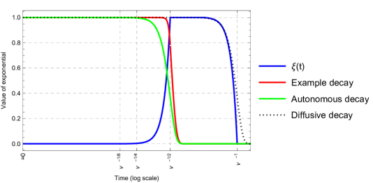
Figure 2: Plot of the exponential decay in Example B, compared to $\xi(t)=1$ and pure diffusion as references, all without logarithmic corrections, with $k=1$ and $\nu=10^{-10}$.

The second balance governs the gradient norm’s growth. For enhanced dissipation to occur, the gradient’s time derivative must be positive for some time. However, by the first balance, it cannot remain positive indefinitely, as gradients eventually decay. This necessitates at least one sign change in the rate of growth, as noted for specific examples in [24, Fig. 4], [25, Fig. 3] and [3, Fig. 2]. Here, the first term on the right is strictly negative, so any gradient growth must stem from the sign-indefinite term, tied to the transport operator and modulated by $\xi(t)$. Increasing $\xi(t)$ accelerates growth, while decreasing $\xi(t)$ dampens it.

In summary, larger gradients yield faster norm decay via the first balance. Since gradient growth depends on $\xi(t)$, peak gradients can be reached earlier for increasing $\xi(t)$ and later (or lower peaks altogether) for decreasing $\xi(t)$. This heuristic argument is captured precisely in Theorem 1.

In order to accommodate functions that might not be bounded from below or might be intermittent (meaning, switching on and off at some intervals in time), we prove

Theorem 2.

Let $\nu\ll 1$ and $\Theta$ be a solution of (1.7) with $\hat{\Theta}_{0}$ in $L^{2}(\mathbb{T})$. Suppose that $v:\mathbb{T}\rightarrow\mathbb{R}$ is a $C^{2}$ function admitting only a finite amount of simple critical points (i.e. satisfying (1.4)). Suppose that $\xi(t)$ satisfies

$$\xi(t)\leq 1,\quad\xi^{\prime}(t)\leq{C_{\xi}}(\nu\absolutevalue{k})^{1/2},$$ (1.16)

for some small constant $C_{\xi}$. Then for each $\nu$ and $k$ there exists a $C_{\xi}\geq\frac{\nu}{\absolutevalue{k}}$ such that the $L^{2}$ decay estimate

$$\|\hat{\Theta}(t)\|_{L^{2}}^{2}\leq C_{\rm{ed}}\quantity(1+\quantity(\frac{\absolutevalue{k}}{\nu})^{1/2})\exp\left(-C_{\xi}^{\prime}(\nu\absolutevalue{k})^{\frac{1}{2}}\int_{0}^{t}\xi(\tau)^{3}\,d\tau-\nu k^{2}t\right)\norm{\hat{\Theta}_{0}}_{L^{2}}^{2}$$ (1.17)

holds for any $t\leq T$ where the time $T$ is arbitrary but finite and $C_{\rm{ed}},C_{\xi}^{\prime}$ are some constants independent of $\nu,k$.

The value of this theorem is to provide the energy decay estimate for intermittent velocity fields. In Section 3.2, we will discuss in details velocities of the type $\xi(t)v(y)$ where

$$\xi_{A}(t)=\begin{cases}\nu^{\frac{1}{2}}t,&t\in\quantity[0,\frac{1}{\nu^{\frac{1}{2}}}],\\ (1+\nu^{\frac{1}{4}}(t-\frac{1}{\nu^{\frac{1}{2}}}))^{4},&t\in\quantity[\frac{1}{\nu^{\frac{1}{2}}},\frac{1}{\nu^{\frac{3}{4}}}].\end{cases}\quad\text{and}\quad\xi_{B}(t)=\begin{cases}\nu^{1/2}t,&t\in\quantity[0,\frac{1}{\nu^{1/2}}],\\ 1,&t\in\quantity[\frac{1}{\nu^{\frac{1}{2}}},\frac{1}{\nu^{\frac{3}{4}}}],\\ \frac{\nu t-1}{\nu^{\frac{1}{4}}-1},&t\in\quantity[\frac{1}{\nu^{\frac{3}{4}}},\frac{1}{\nu}].\end{cases}$$

The flow corresponding to $\xi_{A}$ exemplifies a transition from a slow flow amenable to Theorem 2 to a fast flow satisfying the assumptions of Theorem 1. We demonstrate that the decay rate in this setting can be derived via a “gluing” argument. Meanwhile, the flow corresponding to $\xi_{B}$ serves as an illustrative example of a velocity profile that activates initially, remains constant over a specified interval, and then deactivates, reflecting a typical scenario in laboratory mixers. As we will demonstrate in Section 3.2, applying Theorem 1/Theorem 2 to these profiles results in a decay rate that differs only slightly from the rate observed in the autonomous case of $\xi(t)=1$. These differences are primarily reflected in lower-order corrections producing small scaling variations, which emerge only after most of the energy has already dissipated. Furthermore, for the flow corresponding to $\xi_{B}$, we observe that the exact shape of the turn-off function has little influence on the dissipation rate after the enhanced dissipation timescale is reached.

To provide another example, in the time interval $[0,\frac{1}{\nu}]$ we consider $\xi(t)=e^{-t}$. While Theorem 1 does not apply, since this function is only bounded from below by the $\nu$-dependent function $e^{-\frac{1}{\nu}}$, it satisfies (1.16) and therefore Theorem 2 is applicable.

This then yields, as expected, a slowed dissipation rate compared to the autonomous case.

The rest of the paper is devoted to the proof of the main results: Theorem 1 is proven in Section 2, while Section 3 is devoted to the proof of Theorem 2 and to the computations of the rates of some intermittent flows.

2 Enhanced dissipation for time-dependent velocity fields of product type

We consider velocity fields

$$\bm{u}(x,y,t)=(\xi(t)v(y),0)^{T},$$ (2.1)

for which the advection-diffusion equation (1.1) reduces to

$$\partial_{t}\Theta+\xi(t)v(y)\partial_{x}\Theta-\nu\Delta\Theta=0\,.$$ (2.2)

We assume

$$\int_{\mathbb{T}}\Theta_{0}(x,y)\,dx=0\quad\mbox{ for all }y\in\mathbb{T}$$ (2.3)

implying

$$\int_{\mathbb{T}}\Theta(x,y)\,dx=0\quad\mbox{ for all }y\in\mathbb{T}$$ (2.4)

since these preserved are conserved through the evolution. As outlined in the introduction, the structure of the shear flow and the domain’s periodicity make it natural to transition to the Fourier transform in $x$, leading to the equation

$$\partial_{t}\hat{\Theta}+\xi(t)v(y)ik\hat{\Theta}=\nu(-k^{2}+\partial_{y}^{2})\hat{\Theta},$$ (2.5)

where $\hat{\Theta}(k,y,t)=\frac{1}{2\pi}\int_{\mathbb{T}}\Theta(x,y,t)e^{-ikx}\,dx$ are the Fourier coefficients in the Fourier series expansion $\Theta(x,y,t)=\sum_{k\neq 0}\hat{\Theta}(y,t)e^{ikx}$. By the transformation

$$\hat{\Theta}(k,y,t)=e^{-\nu k^{2}t}\theta(k,y,t),\quad k\in\mathbb{Z},\quad y\in\mathbb{T},\quad t>0$$

equation turns (2.5) into the hypoelliptic equation

$$\begin{array}[]{rrl}\partial_{t}\theta+\xi(t)v(y)ik\theta&=&\nu\partial_{y}^{2}\theta\,,\\ \theta(x,y,0)&=&\theta_{0}(x,y)\,,\end{array}$$ (2.6)

which hides the horizontal diffusion term $-\nu k^{2}\hat{\Theta}$.
In the rest, for two complex valued functions $\phi,\psi$, we will denote with

$$\langle{\phi},{\psi}\rangle=\int_{\mathbb{T}}\phi\bar{\psi}dy.$$ (2.7)

the standard inner product in $L^{2}(\mathbb{T})$.

We begin by introducing the augmented functional

$$\Phi\coloneqq\frac{1}{2}\bigl{[}E_{0}(t)\;+\;\alpha_{0}(w_{\nu}(t))^{3}E_{1}(t)\;+\;2\beta_{0}(w_{\nu}(t))^{2}E_{3}(t)\;+\;\gamma_{0}w_{\nu}(t)k^{2}E_{4}(t)\bigr{]},$$ (2.8)

where

$$E_{0}(t)=\|\theta(\cdot,t)\|_{L^{2}}^{2},\qquad E_{1}(t)=\|\partial_{y}\theta(\cdot,t)\|_{L^{2}}^{2},\qquad E_{2}(t)=\|\partial_{y}^{2}\theta(\cdot,t)\|_{L^{2}}^{2},$$ (2.9)

$$E_{3}(t)=\real\langle ik\partial_{y}v\theta(\cdot,t),\partial_{y}\theta(\cdot,t)\rangle,\qquad E_{4}(t)=\|\partial_{y}v\,\theta(\cdot,t)\|_{L^{2}}^{2}.$$

The time-dependent weights, parametrized by $\nu$, are defined as

$$w_{\nu}(t)=\frac{1}{1+\nu^{s}t},\quad\text{for some fixed }s\in[0,\infty).$$ (2.10)

As we will see later in the proof of Theorem 1, these weights are carefully chosen to counteract the (potentially) increasing values of $\xi(t)$ over time. They satisfy the relation

$$\frac{d}{dt}(w_{\nu}(t)^{n})=-n\,\nu^{s}w_{\nu}(t)^{n+1},\quad\text{for all }n\in\mathbb{N}.$$ (2.11)

Before we move on, we want to briefly discuss the structure of the weights. The crucial property of the weights is their decay, as captured in (2.11). The exact polynomial structure on the other hand was chosen to introduce this method via the most simple case, and we expect that there may exist others that work similarly. The parameter $s$ allows us to control the bounds of Theorem 1 in terms of timescales measured in powers of the viscosity. This is convenient, as enhanced dissipation and diffusion are usually measured in terms of these scales.

The goal is to show that the functional $\Phi$ satisfies an estimate of the type (see Lemma 2.2)

$$\frac{d}{dt}\Phi(t)\lesssim-(\xi(t)\nu|k|)^{\frac{1}{2}}w_{\nu}(t)\Phi(t)\qquad\mbox{ for any}\quad t\leq T\,.$$

This will yield our result upon the application of Grönwall’s Inequality.

For the moment, the coefficients $\alpha_{0}$, $\beta_{0}$, and $\gamma_{0}$ are arbitrary but must satisfy the following inequality:

$$\frac{\beta_{0}^{2}}{\alpha_{0}}\leq\frac{\gamma_{0}}{16}.$$ (2.12)

Notice that functional $\Phi$ is coercive in the following sense

$$\frac{1}{8}\quantity(4E_{0}+3\alpha_{0}w_{\nu}^{3}E_{1}+3\gamma_{0}k^{2}w_{\nu}E_{4})\leq\Phi\leq\frac{1}{8}\quantity(4E_{0}+5\alpha_{0}w_{\nu}^{3}E_{1}+5\gamma_{0}k^{2}w_{\nu}E_{4}).$$ (2.13)

Using relation (2.12), this is obtained by a direct application of the Cauchy-Schwarz and Young’s inequalities as

$$2\beta_{0}w_{\nu}^{2}\lvert E_{3}\rvert\leq\frac{\alpha_{0}}{4}w_{\nu}^{3}E_{1}+\frac{4\beta_{0}^{2}k^{2}}{\alpha_{0}}w_{\nu}E_{4}\leq\frac{\alpha_{0}}{4}w_{\nu}^{3}E_{1}+\frac{\gamma_{0}k^{2}}{4}w_{\nu}E_{4}.$$

The crucial ingredient, in order to deduce the evolution of the $L^{2}$-norm of the solution, is the following quantitative bound on $\Phi$:

Proposition 2.1.

Let $\nu$ and $k$ such that $\beta\in[\frac{\nu}{|k|},1]$ and assume that $\xi(t)$ satisfies

$$L(t)\leq\xi(t)\leq U(t)$$ (2.14)

where

$$\begin{array}[]{rl}L(t)&=\begin{cases}C^{2}\beta^{2}&\text{for }t\leq t^{*}_{\nu,k}\\ \frac{\nu}{|k|\beta}w_{\nu}(t)^{-2}&\text{for }t\geq t^{*}_{\nu,k}\end{cases}\\[8.0pt] &\quad\text{where}\quad t^{\ast}_{\nu,k}=\frac{1}{\nu^{s}}\left(\frac{|k|^{\frac{1}{2}}C\beta^{\frac{3}{2}}}{\nu^{\frac{1}{2}}}-1\right),\\[10.0pt] U(t)&=w_{\nu}(t)^{-\ell}\\[8.0pt] &\quad\text{for some }\ell\in[2,4]\end{array}$$

with $s\in[0,\infty)$ and some positive constant $C$. Then the energy functional $\Phi(t)$ satisfies the following estimate

$$\Phi(t)\leq\exp\left(-\frac{1}{4}(\beta\nu\absolutevalue{k})^{\frac{1}{2}}\int_{0}^{t}\xi(\tau)^{\frac{1}{2}}w_{\nu}(\tau)\,d\tau\right)\Phi(0)$$

for any $t\leq T$ where the time $T$ is arbitrary but finite.

We now assume Proposition 2.1 to hold and prove Theorem 1.

Proof of Theorem 1.

Following the arguments for the proof in [11,  Corollary 3.3], we introduce the timescale

$$T_{\nu,k}=\frac{1}{\nu^{s^{*}}\absolutevalue{k}^{1/2}},$$ (2.15)

where $s^{*}=\min\{\frac{1}{2},s\}$. The reason for the introduction of this auxiliary $s^{*}$ is purely technical, as it allows a connection to the autonomous setting in the formal limit $s\rightarrow\infty$. It can be avoided if one restricts to $s\leq\frac{1}{2}$.
Upon integration of the energy estimate (2.25), the mean-value theorem ensures the existence of a time $t_{0}\in(0,T_{\nu,k})$, such that

$$2E_{1}(t_{0})=\frac{E_{0}(0)-E_{0}(T_{\nu,k})}{\nu T_{\nu,k}}\leq\nu^{s^{*}-1}\absolutevalue{k}^{1/2}E_{0}(0).$$ (2.16)

This leads to the following bound

$$\alpha_{0}(w_{\nu}(t_{0}))^{3}E_{1}(t_{0})\leq\frac{\nu^{s^{*}-1/2}\beta^{1/2}(w_{\nu}(t_{0}))^{3}}{2}E_{0}(0),$$ (2.17)

where we have used that $\alpha_{0}=(\beta_{0}\nu)^{1/2}$. By (2.13) we then have the estimate

$$\Phi(t_{0}) \leq\frac{1}{8}[4E_{0}(t_{0})+5\alpha_{0}(w_{\nu}(t_{0}))^{3}E_{1}(t_{0})+5\gamma_{0}k^{2}(w_{\nu}(t_{0}))E_{4}(t_{0})]$$ (2.18)

$$\leq K_{0}(1+\nu^{s^{*}-1/2}+\gamma_{0}k^{2})E_{0}(0),$$ (2.19)

where we used again (2.25) to bound $E_{4}(t_{0})\leq\|\partial_{y}v\|_{L^{\infty}}^{2}E_{0}(t_{0})<\|\partial_{y}v\|_{L^{\infty}}^{2}E_{0}(0)$ and that the weight function $w_{\nu}$ is bounded from above by a constant. We emphasize that the constant $K_{0}>0$ is independent of $\nu$ and $k$, but it does depend on $\beta$ and $\lVert\partial_{y}v\rVert_{L^{\infty}}^{2}$. Then, for times $t\in(t_{0},T]$, we apply Proposition 2.1 to find

$$\frac{1}{2}E_{0}(t) \leq\Phi(t)\leq\exp\left(-\frac{1}{4}(\beta\nu\absolutevalue{k})^{\frac{1}{2}}\int_{t_{0}}^{t}\xi(\tau)^{\frac{1}{2}}w_{\nu}(\tau)\,d\tau\right)\Phi(t_{0})$$ (2.20)

and by the above estimate for $\Phi(t_{0})$ we then have

$$\frac{1}{2}E_{0}(t)\leq K_{0}(1+\nu^{s^{*}-1/2}+\gamma_{0}k^{2})\exp\left(\frac{1}{4}(\beta\nu\absolutevalue{k})^{\frac{1}{2}}\int_{0}^{t_{0}}\xi(\tau)^{\frac{1}{2}}w_{\nu}(\tau)\,d\tau\right)\\ \qquad\qquad\qquad\times\exp\left(-\frac{1}{4}(\beta\nu\absolutevalue{k})^{\frac{1}{2}}\int_{0}^{t}\xi(\tau)^{\frac{1}{2}}w_{\nu}(\tau)\,d\tau\right)E_{0}(0)\,,$$

where we wrote $\int_{t_{0}}^{t}=\int_{0}^{t}-\int_{0}^{t_{0}}$.

Now note that for $t\leq t_{0}$ we have the bound

$$w_{\nu}(t)\xi(t)^{\frac{1}{2}}\leq w_{\nu}(t)^{1-\frac{\ell}{2}}\leq 2^{\frac{1}{2}\ell-1}\quad\mbox{ for }\ell>2,$$

where we used that $t_{0}\leq T_{\nu,\ell}=\frac{1}{\nu^{s^{*}}|k|^{\frac{1}{2}}}$ and $|k|\geq 1$. By this upper bound on $t_{0}$ we conclude that

$$\frac{1}{2}E_{0}(t)\leq K_{0}(1+\nu^{s^{*}-1/2}+\gamma_{0}k^{2})\exp\left(\frac{1}{4}\beta^{\frac{1}{2}}\nu^{\frac{1}{2}-s^{\ast}}2^{\frac{1}{2}\ell-1}\right)\\ \times\exp\left(-\frac{1}{4}(\beta\nu\absolutevalue{k})^{\frac{1}{2}}\int_{0}^{t}\xi(\tau)^{\frac{1}{2}}w_{\nu}(\tau)\,d\tau\right)E_{0}(0).$$ (2.21)

We note that the factor of $\nu^{1/2-s^{*}}$ in the second exponential is harmless as $s^{*}\leq\frac{1}{2}$. Similarly, the term $\nu^{s^{*}-1/2}$ in the prefactor can be ignored, as it is at worst ($s^{*}=0$) of the same scaling in $\nu$ as $\gamma_{0}$. ∎

2.1 Proof of Proposition 2.1

Before outlining the strategy used in the proof of Proposition 2.1, we first recall a spectral-gap type inequality as written in [7] (see also [11]).

Lemma 2.1 (Proposition 2.7 in [7]).

Suppose that $v:\mathbb{T}\to\mathbb{R}$ satisfies the assumptions of Theorem 1. Then there exists a constant $C_{sp}\geq 1$ such that for all $\sigma\in(0,1]$,

$$\sigma^{\tfrac{1}{2}}E_{0}\lesssim C_{sp}[\sigma E_{1}+E_{4}]\,.$$ (2.22)

We will frequently use this inequality. For its proof, we refer the reader to [11, Proposition 3.7].

The proof of Proposition 2.1 relies on the following key lemma:

Lemma 2.2.

Under the same assumptions as in Proposition 2.1, the functional $\Phi$ satisfies, for any finite time $T$,

$$\frac{d}{dt}\Phi+\frac{1}{4}(\beta\,\xi(t)\,\nu|k|)^{\tfrac{1}{2}}w_{\nu}(t)\,\Phi\leq 0,\quad\forall t\leq T.$$ (2.23)

Applying Gronwall’s inequality to (2.23) immediately yields Proposition 2.1.

Proof.

We divide the proof in three steps: in the first one we will use energy balances to derive an upper bound on $\Phi$, under specific growth conditions on $\xi(t)$. In the second step, we apply the spectral gap estimate of Lemma 2.1 in order to “eliminate” $E_{0}$ from the upper bound. In the third step, we reconstruct the functional.

Step 1: Functional estimate

We first compute the time derivative of the functional $\Phi$ and find

$$\derivative{t}\Phi=\frac{1}{2}\derivative{t}E_{0}+\frac{1}{2}\alpha_{0}\derivative{t}\quantity(w_{\nu}^{3}E_{1})+\beta_{0}\derivative{t}\quantity(w_{\nu}^{2}E_{3})+\frac{1}{2}\gamma_{0}k^{2}\derivative{t}\quantity(w_{\nu}E_{4}).$$ (2.24)

By standard energy methods we have the following energy balances, whose proofs are provided in Lemma B.1 in the Appendix:

$$\frac{1}{2}\frac{d}{dt}E_{0}(t) =-\nu E_{1}(t),$$ (2.25)

$$\frac{1}{2}\frac{d}{dt}E_{1}(t) =-\nu E_{2}(t)-\xi(t)E_{3}(t),$$ (2.26)

$$\frac{1}{2}\frac{d}{dt}E_{3}(t) =-\tfrac{1}{2}\xi(t)k^{2}E_{4}(t)\;-\;\nu\real\langle ik\partial_{y}v\partial_{y}\theta,\partial_{y}^{2}\theta\rangle\;-\;\tfrac{1}{2}\nu\real\langle ik\partial_{y}^{2}v\theta,\partial_{y}^{2}\theta\rangle,$$ (2.27)

$$\frac{1}{2}\frac{d}{dt}E_{4}(t) =-\nu\|\partial_{y}v\partial_{y}\theta\|_{L^{2}}^{2}\;-\;2\nu\real\langle\partial_{y}v\partial_{y}^{2}v\theta,\partial_{y}\theta\rangle.$$ (2.28)

Thanks to these identities, (2.24) can be rewritten as follows

$$\derivative{t}\Phi-\frac{1}{2}\alpha_{0}E_{1}\derivative{w_{\nu}^{3}}{t}-\beta_{0}E_{3}\derivative{w_{\nu}^{2}}{t}-\frac{1}{2}\gamma_{0}k^{2}E_{4}\derivative{w_{\nu}}{t}$$

$$+\nu E_{1}+\nu\alpha_{0}w_{\nu}^{3}E_{2}+\beta_{0}\xi(t)k^{2}w_{\nu}^{2}E_{4}+\nu\gamma_{0}k^{2}w_{\nu}\norm{\partial_{y}v\partial_{y}\theta}_{L^{2}}^{2}$$

$$= -\alpha_{0}w_{\nu}^{3}\xi(t)E_{3}-2\nu\beta_{0}w_{\nu}^{2}\real\langle{ik\partial_{y}v\partial_{y}\theta},{\partial_{y}^{2}\theta}\rangle-\nu\beta_{0}w_{\nu}^{2}\real\langle{ik\partial_{y}^{2}v\theta},{\partial_{y}^{2}\theta}\rangle$$

$$-2\nu\gamma_{0}k^{2}w_{\nu}\real\langle{\partial_{y}v\partial_{y}^{2}v\theta},{\partial_{y}\theta}\rangle.$$

We first estimate the inner products on the right-hand side by Young’s inequality and get

$$\lvert\alpha_{0}\xi(t)w_{\nu}^{3}E_{3}\rvert \leq\frac{1}{2}\frac{\alpha_{0}^{2}}{\beta_{0}}\xi(t)w_{\nu}^{4}E_{1}+\frac{k^{2}}{2}\beta_{0}\xi(t)w_{\nu}^{2}E_{4},$$

$$\lvert 2\nu\beta_{0}w_{\nu}^{2}\real\langle{ik\partial_{y}v\partial_{y}\theta},{\partial_{y}^{2}\theta}\rangle\rvert \leq\frac{\nu}{2}\alpha_{0}w_{\nu}^{3}E_{2}+2\nu k^{2}\frac{\beta_{0}^{2}}{\alpha_{0}}w_{\nu}\norm{\partial_{y}v\partial_{y}\theta}_{L^{2}}^{2},$$

$$\lvert\nu\beta_{0}w_{\nu}^{2}\real\langle{ik\partial_{y}^{2}v\theta},{\partial_{y}^{2}\theta}\rangle\rvert \leq\frac{\nu}{2}\alpha_{0}w_{\nu}^{3}E_{2}+\frac{\nu k^{2}}{2}\frac{\beta_{0}^{2}}{\alpha_{0}}w_{\nu}\norm{\partial_{y}^{2}v\theta}_{L^{2}}^{2},$$

$$\lvert 2\nu\gamma_{0}k^{2}w_{\nu}\real\langle{\partial_{y}v\partial_{y}^{2}v\theta},{\partial_{y}\theta}\rangle\rvert \leq\frac{\nu k^{2}}{2}\gamma_{0}w_{\nu}\lVert\partial_{y}v\partial_{y}\theta\rVert^{2}+2\gamma_{0}\nu k^{2}w_{\nu}\norm{\partial_{y}^{2}v\theta}_{L^{2}}^{2}.$$

Using these inequalities we can obtain the following estimate for the time derivative of the functional (2.24)

$$\derivative{t}\Phi-\frac{1}{2}\alpha_{0}E_{1}\derivative{w_{\nu}^{3}}{t}-\beta_{0}E_{3}\derivative{w_{\nu}^{2}}{t}-\frac{1}{2}\gamma_{0}k^{2}E_{4}\derivative{w_{\nu}}{t}$$

$$+ \quantity(\nu-\frac{1}{2}\frac{\alpha_{0}^{2}}{\beta_{0}}\xi(t)w_{\nu}^{4})E_{1}+\frac{k^{2}}{2}\beta_{0}\xi(t)w_{\nu}^{2}E_{4}$$

$$\leq \nu k^{2}\quantity(2\frac{\beta_{0}^{2}}{\alpha_{0}}-\frac{\gamma_{0}}{2})w_{\nu}\norm{\partial_{y}v\partial_{y}\theta}_{L^{2}}^{2}+\nu k^{2}w_{\nu}\quantity(\frac{1}{2}\frac{\beta_{0}^{2}}{\alpha_{0}}+2\gamma_{0})\norm{\partial_{y}^{2}v\theta}_{L^{2}}^{2}.$$

Now by using condition (2.12) this estimate can be simplified to

$$\derivative{t}\Phi-\frac{1}{2}\alpha_{0}E_{1}\derivative{w_{\nu}^{3}}{t}-\beta_{0}E_{3}\derivative{w_{\nu}^{2}}{t}-\frac{1}{2}\gamma_{0}k^{2}E_{4}\derivative{w_{\nu}}{t}+\quantity(\nu-\frac{1}{2}\frac{\alpha_{0}^{2}}{\beta_{0}}\xi(t)w_{\nu}^{4})E_{1}+\frac{k^{2}}{2}\beta_{0}\xi(t)w_{\nu}^{2}E_{4}\\ \leq\nu k^{2}c_{\infty}\gamma_{0}w_{\nu}E_{0},$$

where we have used the constraint $3\norm{\partial_{y}^{2}v}^{2}_{L^{\infty}}\leq c_{\infty}$. Next we wish to estimate the terms with time derivatives of the weights and therefore explicitly compute them by using relation (2.11)

$$\derivative{t}\Phi+\alpha_{0}\frac{3\nu^{s}}{2}w_{\nu}^{4}E_{1}+\frac{\nu^{s}}{2}\gamma_{0}k^{2}w_{\nu}^{2}E_{4}+\quantity(\nu-\frac{1}{2}\frac{\alpha_{0}^{2}}{\beta_{0}}\xi(t)w_{\nu}^{4})E_{1}+\frac{k^{2}}{2}\beta_{0}\xi(t)w_{\nu}^{2}E_{4}\\ \leq-2\beta_{0}\nu^{s}w_{\nu}^{3}E_{3}+\nu k^{2}c_{\infty}\gamma_{0}w_{\nu}E_{0}.$$

Similarly to the estimates above, by Young’s inequality we find

$$\lvert 2\beta_{0}\nu^{s}w_{\nu}^{3}E_{3}\rvert \leq\frac{\alpha_{0}}{2}\nu^{s}w_{\nu}^{4}E_{1}+\frac{2\beta_{0}^{2}}{\alpha_{0}}\nu^{s}k^{2}w_{\nu}^{2}E_{4}$$

$$\leq\frac{\alpha_{0}}{2}\nu^{s}w_{\nu}^{4}E_{1}+\frac{k^{2}}{8}\gamma_{0}\nu^{s}k^{2}w_{\nu}^{2}E_{4},$$

where we again used condition (2.12) in the second line.

Now we can absorb these terms into their respective counterparts on the left and subsequentially drop the residuals of these terms. This simplifies the estimate for $\derivative{t}\Phi$ further to

$$\derivative{t}\Phi+\quantity(\nu-\frac{1}{2}\frac{\alpha_{0}^{2}}{\beta_{0}}\xi(t)w_{\nu}^{4})E_{1}+\frac{k^{2}}{2}\beta_{0}\xi(t)w_{\nu}^{2}E_{4}\leq\nu k^{2}c_{\infty}\gamma_{0}w_{\nu}E_{0}.$$

Then, the upper bound in (2.14) and the choice

$$\alpha_{0}=\nu^{\frac{1}{2}}\beta_{0}^{\frac{1}{2}}\,,$$ (2.29)

imply

$$\nu-\frac{1}{2}\frac{\alpha_{0}^{2}}{\beta_{0}}\xi(t)w_{\nu}^{4}\geq\frac{\nu}{4}\xi(t)w_{\nu}^{\ell}.$$

Thus, we obtain

$$\derivative{t}\Phi+\frac{\nu}{4}\left(1+\xi(t)w_{\nu}^{\ell}\right)E_{1}+\frac{k^{2}}{2}\beta_{0}\xi(t)w_{\nu}^{2}E_{4}\leq\nu k^{2}\gamma_{0}c_{\infty}w_{\nu}E_{0}.$$ (2.30)

Step 2: Spectral gap estimate

We start from (2.30) and rearrange it as follows:

$$\derivative{t}\Phi+\frac{\nu}{4}\xi(t)w_{\nu}^{\ell}E_{1}+\frac{k^{2}}{4}\beta_{0}\xi(t)w_{\nu}^{2}E_{4}+A\nu k^{2}\gamma_{0}c_{\infty}w_{\nu}E_{0}\\ +\frac{\nu}{4}E_{1}+\frac{k^{2}}{4}\beta_{0}\xi(t)w_{\nu}^{2}E_{4}\leq(A+1)\nu k^{2}\gamma_{0}c_{\infty}w_{\nu}E_{0}\,,$$

where $A>0$ is a balancing parameter, to be determined. Our goal is to control the bad term caused by diffusion on the right-hand side of the inequality with $E_{1}$ and $E_{4}$. Now we recall the spectral gap estimate from Lemma 2.1, which we rewrite in the form

$$E_{0}\leq C_{sp}[\sigma^{\frac{1}{2}}E_{1}+\sigma^{-\frac{1}{2}}E_{4}],\quad\forall\sigma\in(0,1].$$ (2.31)

If we choose

$$\sigma=\frac{\nu}{k^{2}\beta_{0}\xi(t)w_{\nu}(t)^{2}}\leq 1\qquad\mbox{ and }A=\frac{1}{4}\frac{\beta_{0}^{\frac{1}{2}}\xi(t)^{\frac{1}{2}}\nu^{-\frac{1}{2}}}{\absolutevalue{k}\gamma_{0}c_{\infty}C_{\rm{sp}}}-1\,.$$

then we absorb the right-hand side within parts of the left-hand side of the inequality involving $\Phi$:

$$\derivative{t}\Phi+\frac{\nu}{4}\xi(t)w_{\nu}^{\ell}E_{1}+\frac{k^{2}}{4}\beta_{0}\xi(t)w_{\nu}^{2}E_{4}+A\nu k^{2}\gamma_{0}c_{\infty}w_{\nu}E_{0}\leq 0.$$

On the one hand, we notice that the spectral-gap constraint $\sigma\leq 1$ translates in the time-dependent lower bound for $\xi(t)$

$$\xi(t)\geq\frac{\nu}{k^{2}\beta_{0}w_{\nu}(t)^{2}}=\frac{\nu}{k^{2}\beta_{0}}(1+\nu^{s}t)^{2}$$ (2.32)

On the other hand, we observe that if

$$\xi(t)\geq 25\frac{k^{2}\gamma_{0}^{2}\nu c_{\infty}^{2}C_{\rm{sp}}^{2}}{\beta_{0}}$$ (2.33)

then, without affecting scaling behaviours, we can estimate the above inequality and arrive at

$$\derivative{t}\Phi+\frac{\nu}{4}\xi(t)w_{\nu}^{\ell}E_{1}+\frac{k^{2}}{4}\beta_{0}\xi(t)w_{\nu}^{2}E_{4}+\frac{1}{4}(\beta_{0}\xi(t)\nu)^{\frac{1}{2}}\absolutevalue{k}w_{\nu}\ E_{0}\leq 0\,.$$

Towards the reconstruction of the functional, we rewrite this as

$$\derivative{t}\Phi+\frac{1}{4}(\beta_{0}\xi(t)\nu)^{\frac{1}{2}}\absolutevalue{k}w_{\nu}\quantity[E_{0}+\frac{\nu^{1/2}}{\beta_{0}^{1/2}\absolutevalue{k}}\xi(t)^{1/2}w^{\ell-1}E_{1}+\frac{\absolutevalue{k}}{\nu^{1/2}}\beta_{0}^{1/2}\xi(t)^{1/2}w_{\nu}E_{4}]\leq 0.$$

Now since $w_{\nu}^{\ell-1}\geq w_{\nu}^{3}$ for $\ \leq 4$ we can already restore the proper weights of the functional:

$$\derivative{t}\Phi+\frac{1}{4}(\beta_{0}\xi(t)\nu)^{\frac{1}{2}}\absolutevalue{k}w_{\nu}\quantity[E_{0}+\frac{\nu^{1/2}}{\beta_{0}^{1/2}\absolutevalue{k}}\xi(t)^{1/2}w_{\nu}^{3}E_{1}+\frac{\absolutevalue{k}}{\nu^{1/2}}\beta_{0}^{1/2}\xi(t)^{1/2}w_{\nu}E_{4}]\leq 0.$$ (2.34)

Step 3: Rebuilding the functional
We are left with restoring the correct parameters of the functional and dealing with the residual powers of $\xi(t)$ in front if $E_{1}$ and $E_{4}$.

Recalling the choice of $\alpha_{0}$ in (2.29), we now choose

$$\gamma_{0}=16\frac{\beta_{0}^{3/2}}{\nu^{1/2}}$$ (2.35)

so that (2.12) is satisfied. Inserting this choice in (2.33) we have

$$\xi(t)\geq 6400k^{2}\beta_{0}^{2}c_{\infty}^{2}C_{sp}^{2}.$$

Further, in order to make the lower bound uniform in $k$, we choose

$$\beta_{0}=\beta\absolutevalue{k}^{-1},\quad\mbox{for some }\beta\in\quantity[\frac{\nu}{\absolutevalue{k}},1]$$ (2.36)

and set $80c_{\infty}C_{sp}=:C$. Now we can rewrite (2.32) as (2.33) as

$$\xi(t)\geq\frac{\nu}{\absolutevalue{k}\beta}(1+\nu^{s}t)^{2},$$ (2.37)

and (2.33) as

$$\xi(t)\geq C^{2}\beta^{2}.$$ (2.38)

Depending on the dominating lower bounds, we identify two regimes:

$$t\leq t^{\ast}_{\nu,k}\quad\mbox{ and }\quad t\geq t^{\ast}_{\nu,k}\qquad\mbox{ where }\quad t^{\ast}_{\nu,k}=\frac{1}{\nu^{s}}\left(\frac{|k|^{\frac{1}{2}}\nu^{\frac{1}{2}}C\beta^{\frac{3}{2}}}{\nu^{\frac{1}{2}}}-1\right)$$

Short-time estimate
Assume $t<t_{\nu,k}^{*}$. Since this is the time interval where the lower bound in (2.38) dominates over the lower bound in (2.37), we find

$$\derivative{t}\Phi+\frac{1}{4}(\beta\xi(t)\nu\absolutevalue{k})^{\frac{1}{2}}w_{\nu}\quantity[E_{0}+\frac{\nu^{1/2}\beta^{1/2}}{\absolutevalue{k}^{1/2}}Cw_{\nu}^{3}E_{1}+\frac{\absolutevalue{k}^{1/2}}{\nu^{1/2}}\beta^{3/2}Cw_{\nu}E_{4}]\leq 0.$$

Recalling our parameter choices (2.29), (2.35) this leads to

$$\derivative{t}\Phi+\frac{1}{4}(\beta\xi(t)\nu\absolutevalue{k})^{\frac{1}{2}}w_{\nu}\quantity[E_{0}+C\alpha_{0}w_{\nu}^{3}E_{1}+\frac{1}{16}k^{2}C\gamma_{0}w_{\nu}E_{4}]\leq 0.$$

Notice that, by a suitable parameter choice, we can always make sure that $\frac{1}{16}C=5c_{\infty}C_{sp}\geq 5$ holds. Hence, we get

$$\derivative{t}\Phi+\frac{1}{4}(\beta\xi(t)\nu\absolutevalue{k})^{\frac{1}{2}}w_{\nu}\quantity[E_{0}+5\alpha_{0}w_{\nu}^{3}E_{1}+5k^{2}\gamma_{0}w_{\nu}E_{4}]\leq 0.$$ (2.39)

Large-time estimate
Assume $t\geq t^{*}$. In this case, $\xi(t)\geq\frac{\nu}{|k|\beta}w_{\nu}(t)^{-2}$ and we can insert this lower bound in (2.34) to obtain

$$\derivative{t}\Phi+\frac{1}{4}(\beta\xi(t)\nu\absolutevalue{k})^{\frac{1}{2}}w_{\nu}\bigg{[}E_{0} +\frac{\nu^{1/2}}{\beta^{1/2}\absolutevalue{k}^{1/2}}\quantity(\frac{\nu}{\absolutevalue{k}\beta})^{1/2}w_{\nu}(t)^{-1}w_{\nu}^{3}E_{1}$$

$$+\frac{\absolutevalue{k}^{1/2}}{\nu^{1/2}}\beta^{1/2}\quantity(\frac{\nu}{\absolutevalue{k}\beta})^{1/2}w_{\nu}(t)^{-1}w_{\nu}E_{4}\bigg{]}\leq 0.$$

We now recall that, in this regime, $\frac{\nu}{|k|\beta}w_{\nu}(t)^{-2}\geq C^{2}\beta^{2}$, implying

$$w_{\nu}^{-1}\geq\quantity(\frac{\absolutevalue{k}\beta}{\nu})^{1/2}C$$

such that

$$\derivative{t}\Phi+\frac{1}{4}(\beta\xi(t)\nu\absolutevalue{k})^{\frac{1}{2}}w_{\nu}\quantity[E_{0}+\frac{\nu^{1/2}\beta^{1/2}}{\absolutevalue{k}^{1/2}}Cw_{\nu}^{3}E_{1}+\frac{\absolutevalue{k}^{1/2}}{\nu^{1/2}}\beta^{3/2}Cw_{\nu}E_{4}]\leq 0.$$

Inserting the parameter choices (2.29) and (2.35) we obtain

$$\derivative{t}\Phi+\frac{1}{4}(\beta\xi(t)\nu\absolutevalue{k})^{\frac{1}{2}}w_{\nu}\quantity[E_{0}+C\alpha_{0}w_{\nu}^{3}E_{1}+k^{2}C\gamma_{0}w_{\nu}E_{4}]\leq 0.$$

Therefore, arguing in the same manner as above,

$$\derivative{t}\Phi+\frac{1}{4}(\beta\xi(t)\nu\absolutevalue{k})^{\frac{1}{2}}w_{\nu}\quantity[E_{0}+5\alpha_{0}w_{\nu}^{3}E_{1}+5k^{2}\gamma_{0}w_{\nu}E_{4}]\leq 0.$$ (2.40)

Lastly, by applying the coercivity of the energy functional given in (2.13) to both estimates we arrive at the statement of the Lemma. ∎

Proposition 2.1 is then directly implied by Lemma 2.2.

3 Enhanced dissipation for intermittent velocity fields

In this section, we treat velocity fields that are active at certain times and might be turned off at others. As remarked in the introduction, this class of stirring fields is especially important in applications.
We proceed under the same assumptions outlined in Section 2, specified in (2.1)-(2.7), and continue our analysis of the advection-diffusion equation presented in (2.6).

The starting point is once again an augmented energy functional, albeit with a different modification. It takes the form of

$$\Psi(t)\coloneqq\frac{1}{2}\left[E_{0}(t)+\alpha_{0}(t)E_{1}(t)+2\beta_{0}(t)E_{3}(t)+\gamma_{0}(t)k^{2}E_{4}(t)\right],$$ (3.1)

where $E_{0},E_{1},E_{3},E_{4}$ are defined in (2.9). The choice of this specific form of the functional $\Psi$ will become clear in the arguments that follow. For the moment, we only notice two differences with respect to the energy functional $\Phi$ defined in (2.8): the absence of time-dependent weights and the time-dependency of the balancing parameters $\alpha_{0},\beta_{0}$ and $\gamma_{0}$. The second will be necessary in order to balance the scaling of the various error terms arising in those cases when $\xi(t)$ becomes very small, i.e. scaling with powers of $\nu$. This is crucial as it allows us to avoid lower bounds on $\xi(t)$ and therefore let it go to zero.

We assume that for all times $t\geq 0$ the non-negative parameters $\alpha_{0},\beta_{0},\gamma_{0}$ are bounded, and we impose an analogue condition to (2.12):

$$\beta_{0}(t)^{2}\leq\frac{1}{16}\gamma_{0}(t)\alpha_{0}(t)$$ (3.2)

Note that the coercivity of the augmented energy functional $\Psi$ follows from the point-wise in time bound (3.2). By the same strategy employed to derive (2.13), we find

$$\frac{1}{8}\quantity(4E_{0}+3\alpha_{0}(t)E_{1}(t)+3\gamma_{0}(t)k^{2}E_{4}(t))\leq\Psi(t)\leq\frac{1}{8}\quantity(4E_{0}(t)+5\alpha_{0}(t)E_{1}(t)+5\gamma_{0}(t)k^{2}E_{4}(t)).$$ (3.3)

In order to prove Theorem 2 we first need to derive a quantitative bound for the functional $\Psi(t)$. This is the contained in the next proposition.

Proposition 3.1.

Assume that $\xi(t)$ satisfies the conditions

$$\xi(t)\leq 1,\quad\xi^{\prime}(t)\leq{C_{\xi}}(\nu\absolutevalue{k})^{1/2},$$ (3.4)

for some small constant $C_{\xi}$. Then there exists a constant $C_{\xi}^{\prime}$ that may only depend on $\norm{\partial_{y}^{2}v(y)}_{L^{\infty}}$ such that the energy functional $\Psi$ satisfies the following estimate

$$\Psi(t)\leq\exp\quantity(-C_{\xi}^{\prime}(\nu\absolutevalue{k})^{1/2}\int_{0}^{t}\xi(\tau)^{3}d\tau)\Psi(0)$$ (3.5)

for any $t\leq T$ where the time $T$ is arbitrary but finite.

We now assume Proposition 3.1 and prove Theorem 2.

Proof of Theorem 2.

We introduce the timescale

$$T_{\nu,k}=\frac{1}{\nu^{1/2}\absolutevalue{k}^{1/2}},$$ (3.6)

and, in analogy with the analysis in Section 2 we define

$$\alpha_{0}(t)=\nu^{1/2}\beta_{0}(t)^{1/2},\quad\beta_{0}(t)=\beta(t)\absolutevalue{k}^{-1}.$$ (3.7)

Upon integrating the energy estimate (2.25), the mean-value theorem ensures the existence of a time $t_{0}\in(0,T_{\nu,k})$, such that

$$2E_{1}(t_{0})=\frac{E_{0}(0)-E_{0}(T_{\nu,k})}{\nu T_{\nu,k}}\leq\nu^{-1/2}\absolutevalue{k}^{1/2}E_{0}(0).$$ (3.8)

This leads to the following bound

$$\alpha_{0}(t_{0})E_{1}(t_{0})\leq\frac{\beta(t_{0})^{1/2}}{2}E_{0}(0),$$ (3.9)

where we have used that $\alpha_{0}=(\beta_{0}\nu)^{1/2}$.
By (3.3) we then have the estimate

$$\Phi(t_{0}) \leq\frac{1}{8}[4E_{0}(t_{0})+5\alpha_{0}(t_{0})E_{1}(t_{0})+5\gamma_{0}(t_{0})k^{2}E_{4}(t_{0})]$$

$$\leq K_{0}(1+\beta(t_{0})^{1/2}+\gamma_{0}(t_{0})k^{2})E_{0}(0),$$

where we used again (2.25) to bound $E_{4}(t_{0})\leq\|\partial_{y}v\|_{L^{\infty}}^{2}E_{0}(t_{0})<\|\partial_{y}v\|_{L^{\infty}}^{2}E_{0}(0)$. We emphasize that the constant $K_{0}>0$ is independent of $\nu$ and $k$, but it does depend on $\lVert\partial_{y}v\rVert_{L^{\infty}}^{2}$. Then, for times $t\in(t_{0},T]$, we apply Proposition 2.1 to find

$$\frac{1}{2}E_{0}(t) \leq\Phi(t)\leq\exp\left(-C_{\xi}^{\prime}(\nu\absolutevalue{k})^{\frac{1}{2}}\int_{t_{0}}^{t}\xi(\tau)^{3}\,d\tau\right)\Phi(t_{0})$$ (3.10)

and by the above estimate for $\Phi(t_{0})$ we then have

$$\frac{1}{2}E_{0}(t)\leq K_{0}(1+\beta(t_{0})^{1/2}+\gamma_{0}(t_{0})k^{2})\exp\left(C_{\xi}^{\prime}(\nu\absolutevalue{k})^{\frac{1}{2}}\int_{0}^{t_{0}}\xi(\tau)^{3}\,d\tau\right)\\ \qquad\qquad\qquad\times\exp\left(-C_{\xi}^{\prime}(\nu\absolutevalue{k})^{\frac{1}{2}}\int_{0}^{t}\xi(\tau)^{3}\,d\tau\right)E_{0}(0)\,,$$

where we wrote $\int_{t_{0}}^{t}=\int_{0}^{t}-\int_{0}^{t_{0}}$.
Using that $t_{0}\leq T_{\nu,k}=(\nu|k|)^{-\frac{1}{2}}$ we conclude

$$\frac{1}{2}E_{0}(t)\leq K_{0}(1+\beta(t_{0})^{1/2}+\gamma_{0}(t_{0})k^{2})\exp\left(C_{\xi}^{\prime}\right)\\ \times\exp\left(-C_{\xi}^{\prime}(\nu\absolutevalue{k})^{\frac{1}{2}}\int_{0}^{t}\xi(\tau)^{3}\,d\tau\right)E_{0}(0).$$ (3.11)

∎

3.1 Proof of Proposition 3.1

The proof of Proposition 3.1 is a direct consequence of the following

Lemma 3.1.

Under the same assumptions of Proposition (3.1), the functional $\Phi$ satisfies the following estimate

$$\derivative{t}\Psi+C_{\xi}^{\prime}(\nu\absolutevalue{k})^{1/2}\xi(t)^{3}\Psi \leq 0,\quad\forall t\leq T,$$ (3.12)

where time $T$ is arbitrary but finite.

This Lemma, when combined with an application of Grönwall’s inequality, implies Proposition 3.1.

Proof.

In structural analogy to the proof of Lemma 2.23, we divide the proof in three steps: in the first one we will use energy balances to derive an upper bound on $\Phi$, where we now need to control additional error terms arising from the time-dependency of $\beta$. In the second step, we apply the spectral gap estimate of Lemma 2.1 in order to ”eliminate” $E_{0}$ from the upper bound. In the third step, we reconstruct the functional.
Step 1: Functional estimate

We first compute the time derivative of the functional $\Phi$ and find

$$\derivative{t}\Psi(t)=\frac{1}{2}\derivative{t}E_{0}(t)+\frac{1}{2}\derivative{t}\quantity(\alpha_{0}(t)E_{1}(t))+\derivative{t}\quantity(\beta_{0}(t)E_{3}(t))+\frac{1}{2}k^{2}\derivative{t}\quantity(\gamma_{0}(t)E_{4}(t)).$$ (3.13)

Using the above energy identities (see Lemma B.1) this can be rewritten as follows

$$\derivative{t}\Psi-\frac{1}{2}\derivative{\alpha_{0}}{t}E_{1}-\derivative{\beta_{0}}{t}E_{3}-\frac{1}{2}k^{2}\derivative{\gamma_{0}}{t}E_{4}$$

$$+\nu E_{1}+\nu\alpha_{0}E_{2}+\beta_{0}\xi(t)k^{2}E_{4}+\nu\gamma_{0}k^{2}\norm{\partial_{y}v\partial_{y}\theta}_{L^{2}}^{2}$$

$$= -\alpha_{0}\xi(t)E_{3}-2\nu\beta_{0}\real\langle{ik\partial_{y}v\partial_{y}\theta},{\partial_{y}^{2}\theta}\rangle-\nu\beta_{0}\real\langle{ik\partial_{y}^{2}v\theta},{\partial_{y}^{2}\theta}\rangle$$

$$-2\nu\gamma_{0}k^{2}w_{\nu}\real\langle{\partial_{y}v\partial_{y}^{2}v\theta},{\partial_{y}\theta}\rangle.$$

We estimate the inner products on the right-hand side by means of Young’s inequality and get

$$\lvert\alpha_{0}\xi(t)E_{3}\rvert \leq\frac{1}{2}\frac{\alpha_{0}^{2}}{\beta_{0}}\xi(t)E_{1}+\frac{k^{2}}{2}\beta_{0}\xi(t)E_{4},$$

$$\lvert 2\nu\beta_{0}\real\langle{ik\partial_{y}v\partial_{y}\theta},{\partial_{y}^{2}\theta}\rangle\rvert \leq\frac{\nu}{2}\alpha_{0}E_{2}+2\nu k^{2}\frac{\beta_{0}^{2}}{\alpha_{0}}\norm{\partial_{y}v\partial_{y}\theta}_{L^{2}}^{2},$$

$$\lvert\nu\beta_{0}\real\langle{ik\partial_{y}^{2}v},{\partial_{y}^{2}\theta}\rangle\rvert \leq\frac{\nu}{2}\alpha_{0}E_{2}+\frac{\nu k^{2}}{2}\frac{\beta_{0}^{2}}{\alpha_{0}}\norm{\partial_{y}^{2}v\theta}_{L^{2}}^{2},$$

$$\lvert 2\nu\gamma_{0}k^{2}\real\langle{\partial_{y}v\partial_{y}^{2}v\theta},{\partial_{y}\theta}\rangle\rvert \leq\frac{\nu k^{2}}{2}\gamma_{0}\lVert\partial_{y}v\partial_{y}\theta\rVert^{2}+2\gamma_{0}\nu k^{2}\norm{\partial_{y}^{2}v\theta}_{L^{2}}^{2},$$

from which one obtains the following estimate for the time derivative of the functional (3.13)

$$\derivative{t}\Psi-\frac{1}{2}\derivative{\alpha_{0}}{t}E_{1}-\derivative{\beta_{0}}{t}E_{3}-\frac{1}{2}k^{2}\derivative{\gamma_{0}}{t}E_{4}$$

$$+ \quantity(\nu-\frac{1}{2}\frac{\alpha_{0}^{2}}{\beta_{0}}\xi(t))E_{1}+\frac{k^{2}}{2}\beta_{0}\xi(t)E_{4}$$

$$\leq \nu k^{2}\quantity(2\frac{\beta_{0}^{2}}{\alpha_{0}}-\frac{\gamma_{0}}{2})\norm{\partial_{y}v\partial_{y}\theta}_{L^{2}}^{2}+\nu k^{2}\quantity(\frac{1}{2}\frac{\beta_{0}^{2}}{\alpha_{0}}+2\gamma_{0})\norm{\partial_{y}^{2}v\theta}_{L^{2}}^{2}.$$

Now by using conditions (3.2), (3.7) and the fact that $\xi(t)\leq 1$, this estimate can be simplified to

$$\derivative{t}\Psi-\frac{1}{2}\derivative{\alpha_{0}}{t}E_{1}-\derivative{\beta_{0}}{t}E_{3}-\frac{1}{2}k^{2}\derivative{\gamma_{0}}{t}E_{4}$$

$$+ \frac{\nu}{2}E_{1}+\frac{k^{2}}{2}\beta_{0}\xi(t)E_{4}$$

$$\leq 3\nu k^{2}\gamma_{0}\norm{\partial_{y}^{2}v\theta}_{L^{2}}^{2}\leq\nu k^{2}c_{\infty}\gamma_{0}E_{0},$$

where we have used the constraint $c_{\infty}\geq 3\norm{\partial_{y}^{2}v}^{2}_{L^{\infty}}$. Now we face the issue that the sign of the derivatives of the parameters in the first line is not determined. Hence, we need to be able to control all additional terms. In order to do this, we now need to assume a specific form on $\beta$. We choose

$$\beta(t)=C_{\xi}\xi(t)^{2}.$$ (3.14)

The exact form of the constant $C_{\xi}\leq 1$ will be determined later.

This choice together with the formulas for the parameters (3.7) and the choice

$$\gamma_{0}(t)=16\frac{\beta_{0}(t)^{3/2}}{\nu^{1/2}}$$ (3.15)

yield

$$\derivative{t}\Psi -\frac{\nu^{1/2}}{2\absolutevalue{k}^{1/2}}C_{\xi}^{1/2}\xi^{\prime}(t)E_{1}-2\absolutevalue{k}^{-1}C_{\xi}\xi^{\prime}(t)\xi(t)E_{3}-\frac{48}{2\nu^{1/2}}\absolutevalue{k}^{1/2}C_{\xi}^{3/2}\xi^{\prime}(t)\xi(t)^{2}E_{4}$$

$$+\frac{\nu}{2}E_{1}+\frac{k^{2}}{2}\beta_{0}\xi(t)E_{4}\leq\nu k^{2}c_{\infty}\gamma_{0}E_{0}.$$

Now we consider the error terms of the first line separately to find by Young’s inequality that

$$-\quantity[\frac{\nu^{1/2}}{2}C_{\xi}^{1/2}\absolutevalue{k}^{-1/2}\xi^{\prime}(t)E_{1}+2C_{\xi}\absolutevalue{k}^{-1}\xi^{\prime}(t)\xi(t)E_{3}+\frac{48\absolutevalue{k}^{1/2}}{2\nu^{1/2}}C_{\xi}^{3/2}\xi^{\prime}(t)\xi(t)^{2}E_{4}]$$

$$= -\quantity[\frac{\nu^{1/2}}{2}C_{\xi}^{1/2}\absolutevalue{k}^{-1/2}\xi^{\prime}(t)E_{1}+2C_{\xi}\xi^{\prime}(t)\xi(t)\real\langle i\partial_{y}v\theta,\partial_{y}\theta\rangle+\frac{48\absolutevalue{k}^{1/2}}{2\nu^{1/2}}C_{\xi}^{3/2}\xi^{\prime}(t)\xi(t)^{2}E_{4}]$$

$$\geq -\quantity[\frac{5}{2}\nu^{1/2}C_{\xi}^{1/2}\absolutevalue{k}^{-1/2}\xi^{\prime}(t)E_{1}+25\frac{\absolutevalue{k}^{1/2}}{\nu^{1/2}}C_{\xi}^{3/2}\xi^{\prime}(t)\xi(t)^{2}E_{4}].$$

Then

$$\derivative{t}\Psi+\left[\frac{\nu}{2}-\frac{5}{2}\nu^{1/2}C_{\xi}^{1/2}\absolutevalue{k}^{-1/2}\xi^{\prime}(t)\right]E_{1}+\left[\frac{k^{2}}{2}\beta_{0}\xi(t)-25\frac{\absolutevalue{k}^{1/2}}{\nu^{1/2}}C_{\xi}^{3/2}\xi^{\prime}(t)\xi(t)^{2}\right]E_{4}$$

$$\leq\nu k^{2}c_{\infty}\gamma_{0}E_{0}.$$

implies

$$\derivative{t}\Psi+\frac{\nu}{4}E_{1}+\frac{k^{2}}{4}\beta_{0}\xi(t)E_{4}\leq\nu k^{2}c_{\infty}\gamma_{0}E_{0}$$ (3.16)

if the two conditions

$$\frac{5}{2}\nu^{1/2}C_{\xi}^{1/2}\absolutevalue{k}^{-1/2}\xi^{\prime}(t) \leq \frac{\nu}{4}$$ (3.17)

$$25\frac{\absolutevalue{k}^{1/2}}{\nu^{1/2}}C_{\xi}^{3/2}\xi^{\prime}(t)\xi(t)^{2} \leq \frac{k^{2}}{4}\beta_{0}\xi(t)=\frac{k^{2}}{4}|k|^{-1}C_{\xi}\xi(t)^{2}\xi(t)$$ (3.18)

are simultaneously satisfied. Since $\xi\leq 1$, this is the case when

$$\xi^{\prime}(t)\leq\frac{1}{100}C_{\xi}^{-\frac{1}{2}}|k|^{\frac{1}{2}}\nu^{\frac{1}{2}}\,.$$ (3.19)

Notice that, for the sake of clarity of the argument, we did not try to optimize on numerical constants at any point.

Step 2: Spectral gap estimate
We start from (3.16) and rearrange it as follows:

$$\derivative{t}\Psi+\frac{\nu}{8}E_{1}+\frac{k^{2}}{8}\beta_{0}\xi(t)E_{4}+\frac{\nu}{8}\xi(t)^{3}E_{1}+\frac{k^{2}}{8}\beta_{0}\xi(t)E_{4}+A\nu k^{2}c_{\infty}\gamma_{0}E_{0}\leq(A+1)\nu k^{2}c_{\infty}\gamma_{0}E_{0}$$

where $A>0$ is a balancing parameter to be determined, and we used again that $\xi(t)\leq 1$. Now we recall the spectral gap estimate from Lemma 2.1, which we rewrite in the form

$$E_{0}\leq C_{sp}[\sigma^{\frac{1}{2}}E_{1}+\sigma^{-\frac{1}{2}}E_{4}]\quad\forall\sigma\in(0,1].$$ (3.20)

If we choose

$$\sigma=\frac{\nu}{\absolutevalue{k}C_{\xi}}\leq 1\qquad\mbox{ and }A=\frac{1}{128C_{\xi}c_{\infty}C_{sp}}-1\,.$$

then we absorb the right-hand side with parts of the left-hand side of the inequality involving $\Psi$:

$$\derivative{t}\Psi+\frac{\nu}{8}E_{1}+\frac{k^{2}}{8}\beta_{0}\xi(t)E_{4}+A\nu k^{2}\gamma_{0}c_{\infty}E_{0} \leq 0$$

Now, using the definition of $\gamma_{0}$ in (3.15) and taking $C_{\xi}$ to be small enough such that $C_{\beta}\leq\frac{1}{128}C_{\infty}C_{\rm{sp}}$ , we then get

$$\derivative{t}\Psi+\frac{\nu}{8}E_{1}+\frac{k^{2}}{8}\beta_{0}\xi(t)E_{4}+C_{\xi}^{\prime}(\nu\absolutevalue{k})^{1/2}\xi(t)^{3}E_{0} \leq 0,$$ (3.21)

where $C_{\beta}^{\prime}=16AC_{\beta}^{\frac{3}{2}}c_{\infty}$.

It is crucial that this time we do not have a dependency on $\xi(t)$ in $\sigma$ or $A$, therefore we do not obtain a lower bound and hence can allow it to go to zero.
From here we can directly move to the closing step.
Step 3: Rebuilding the functional
We rewrite (3.21) as

$$\derivative{t}\Psi+C_{\xi}^{\prime}(\nu\absolutevalue{k})^{1/2}\xi(t)^{3}\quantity[E_{0}+\frac{\nu^{1/2}}{\absolutevalue{k}^{1/2}C_{\xi}\xi(t)^{3}}E_{1}+\frac{\absolutevalue{k}^{1/2}}{\nu^{1/2}\xi(t)}E_{4}] \leq 0$$ (3.22)

$$\iff\derivative{t}\Psi+C_{\xi}^{\prime}(\nu\absolutevalue{k})^{1/2}\xi(t)^{3}\quantity[E_{0}+\frac{1}{C_{\xi}^{3/2}\xi(t)^{4}}\alpha_{0}E_{1}+\frac{k^{2}}{16C_{\xi}^{3/2}\xi(t)^{4}}\gamma_{0}E_{4}] \leq 0.$$ (3.23)

Since $\xi(t)\leq 1$, we choose a suitable constant $C_{\xi}$ such that $(16C_{\xi}^{3/2}\xi(t)^{4})^{-1}\geq 5$ and hence

$$\derivative{t}\Psi+C_{\xi}^{\prime}(\nu\absolutevalue{k})^{1/2}\xi(t)^{3}\quantity[E_{0}+5\alpha_{0}E_{1}+5k^{2}\gamma_{0}E_{4}] \leq 0.$$ (3.24)

From this, the statement of the lemma follows directly by coercivity of the energy functional. ∎

3.2 Illustrative examples of intermittent flows

In this section, we examine examples of intermittent flows, which are induced by velocity fields that can be switched on and off at different time intervals. We present two examples: the first involves a velocity field that features a very slow switch on phase and then transitions continuously into a fast polynomial profile. This profile requires a gluing argument to alternate between Theorems 2 and 1. The second example features a slowly varying flow that is gradually switched on, held constant for a period, and then switched off. This case is fully addressed by Theorem 2, and the decay rate can be directly computed from the upper bound in (1.17).

Flows that alternate between the regimes of Theorems 1 and 2 can be handled by employing a “gluing” approach. Specifically, we will use the end state of one estimate as the initial data for the next. Before presenting a concrete example, we will clarify this procedure in an abstract framework:
Assume $t_{0}=0$ and that we have identified times $t_{i}$, for $i=1,\dots,N$ such that on each interval $T_{i}=[t_{i-1},t_{i}]$, are either in the regime of Theorem 2 or Theorem 1. Our goal here is to determine the dissipation rate in terms of the viscosity without focusing on optimisation of the constants. Therefore, we do not track them explicitly and they can change from line to line. We begin by applying results consecutively in the interval $[t_{N-2},t_{N}]=[t_{N-2},t_{N-1}]\cup[t_{N-1},t_{N}]$ , we find that for the final time $t_{N}$ we have

$$E_{0}(t_{N}) \leq K_{N}e^{-C_{N}(\nu\absolutevalue{k})^{1/2}\int_{T_{N}}\xi_{N}(\tau)\,d\tau}E_{0}(t_{N-1})$$

$$\leq K_{N}K_{N-1}\,e^{-C_{N}(\nu\absolutevalue{k})^{1/2}\int_{T_{N}}\xi_{N}(\tau)\,d\tau}\,e^{-C_{N-1}(\nu\absolutevalue{k})^{1/2}\int_{T_{N-1}}\xi_{N-1}(\tau)\,d\tau}E_{0}(t_{N-2})$$

$$=K_{N}K_{N-1}\,e^{-(C_{N}\int_{T_{N}}\xi_{N}(\tau)\,d\tau+C_{N-1}\int_{T_{N-1}}\xi_{N-1}(\tau)\,d\tau)(\nu\absolutevalue{k})^{1/2}}E_{0}(t_{N-2}).$$

Here the $K_{i}$ incorporate all respective prefactors such as the logarithmic corrections, $C_{i}$ are the general constants in the exponential and $\xi_{i}(t)$ is either the weight adjusted $\xi(t)$ (as in Theorem 1) and/or some power of it (as in Theorem 2). The above procedure can be iterated to obtain

$$E_{0}(t_{N}) \leq\Pi_{i}K_{i}e^{-C_{i}(\nu\absolutevalue{k})^{1/2}\int_{T_{i}}\xi_{i}(\tau)d\tau}E_{0}(0)\leq Ke^{-C(\nu\absolutevalue{k})^{1/2}\sum_{i}\int_{T_{i}}\xi_{i}(\tau)d\tau}E_{0}(0)$$

$$=Ke^{-C(\nu\absolutevalue{k})^{1/2}\int_{0}^{T_{N}}\xi^{*}(\tau)d\tau}E_{0}(0),$$

where $K=\max\{K_{i}\}^{N}$, $C=\min\{C_{i}\}$ and $\xi^{*}(t)=\sum_{i}\xi_{i}(t)\bm{1}_{T_{i}}$.
By relabelling, we can write this in the form of a generic $t$ as

$$E_{0}(t)\leq Ke^{-C(\nu\absolutevalue{k})^{1/2}\int_{0}^{t}\xi^{*}(\tau)d\tau}E_{0}(0),\quad\forall t\leq T_{N}.$$ (3.25)

Lastly, we note that at times when a flow is inactive, the decay is purely diffusive and the decay rate is dictated by the Poincaré inequality applied to Lemma B.1.

In order to simplify the notation, we will assume $\absolutevalue{k}=1$ in the following examples.

Example A
Consider the flow

$$\xi_{A}(t)=\xi_{1}(t)\bm{1}_{T_{1}}+\xi_{2}(t)\bm{1}_{T_{2}}$$ (3.26)

with

$$\xi_{1}(t) =\nu^{1/2}t,\,T_{1}=\quantity[0,\frac{1}{\nu^{1/2}}]$$ (3.27)

$$\xi_{2}(t) =(1+\nu^{1/4}(t-\nu^{-1/2}))^{4},\,T_{2}=\quantity[\frac{1}{\nu^{1/2}},\frac{1}{\nu^{3/4}}].$$ (3.28)

This flow begins at zero, growing within the framework of Theorem 2. Upon reaching $\xi(t)=1$ at $t=\frac{1}{\nu^{1/2}}$, it transitions into a phase of polynomial growth, eventually entering the admissible class described in Theorem 1. Consequently, we must bridge the results of these two theorems, necessitating the use of the aforementioned ”gluing” procedure.

We first compute the decay within each interval separately. At the endpoint of the first interval at $t=\frac{1}{\nu^{1/2}}$ we invoke Theorem 2 and find

$$E_{0}\quantity(\frac{1}{\nu^{1/2}})\leq Ke^{-C\nu^{1/2}\int_{0}^{\nu^{-1/2}}\xi_{1}(\tau)^{3}d\tau}E_{0}(0)=Ke^{-\frac{C}{4}}E_{0}(0).$$ (3.29)

At the endpoint of the second interval at $t=\frac{1}{\nu^{3/4}}$ by Theorem 1 we find that

$$E_{0}\quantity(\frac{1}{\nu^{3/4}})=Ke^{-C\nu^{1/2}\int_{\nu^{-1/2}}^{\nu^{-3/4}}\quantity(1+\nu^{1/4}(\tau-\nu^{-1/2}))d\tau}E_{0}(0)=Ke^{-\frac{C}{2}\quantity(\frac{1}{\nu^{3/4}}+\frac{3}{\nu^{1/4}}-\frac{2}{\nu^{1/2}}-2)}E_{0}\quantity(\frac{1}{\nu^{1/2}}).$$ (3.30)

Hence, by the ”gluing” strategy outlined above, we find

$$E_{0}\quantity(\frac{1}{\nu^{3/4}}) \leq Ke^{-\frac{C}{4}}e^{-\frac{C}{2}\quantity(\frac{1}{\nu^{3/4}}+\frac{3}{\nu^{1/4}}-\frac{2}{\nu^{1/2}}-2)}E_{0}(0).$$ (3.31)

For comparison, an autonomous flow $\xi=1$ would have the decay estimate

$$E_{0}\quantity(\frac{1}{\nu^{3/4}}) \leq Ke^{-C\frac{1}{\nu^{1/4}}}E_{0}(0).$$

We find that, while the glued estimate (3.31) includes lower order corrections, the leading order decay at time $t=\frac{1}{\nu^{3/4}}$ is indeed greater than in the autonomous case. However, since the polynomial acceleration happened after the autonomous enhanced dissipation timescale of $t=\frac{1}{\nu^{1/2}}$ was reached, its effect is small. This is because at timescales of order $\mathcal{O}\quantity(\frac{1}{\nu^{3/4}})$ both estimates already scale with negative powers of $\nu$ and therefore in both settings almost all energy is already dissipated at these times. As can be seen from (3.29), the enhanced dissipation timescale mirrors the autonomous case up to a factor of $\frac{1}{4}$.

Example B
We now consider the example given in the introduction. We have

$$\xi_{B}(t)=\xi_{1}(t)\bm{1}_{T_{1}}+\xi_{2}(t)\bm{1}_{T_{2}}+\xi_{3}(t)\bm{1}_{T_{3}}$$ (3.32)

with

$$\xi_{1}(t) =\nu^{1/2}t,\,T_{1}=\quantity[0,\frac{1}{\nu^{1/2}}]$$ (3.33)

$$\xi_{2}(t) =1,\,T_{2}=\quantity[\frac{1}{\nu^{1/2}},\frac{1}{\nu^{3/4}}]$$ (3.34)

$$\xi_{3}(t) =\frac{\nu t-1}{\nu^{1/4}-1},\,T_{3}=\quantity[\frac{1}{\nu^{3/4}},\frac{1}{\nu}].$$ (3.35)

This flow consists of a turn-on phase $T_{1}$, a stationary phase $T_{2}$ and a turn-off phase $T_{3}$. We note that all intervals are in the regime of Theorem 2, and we therefore can compute the decay without gluing. Invoking Theorem 2 we find

$$E_{0}\quantity(\frac{1}{\nu}) \leq Ke^{-C\nu^{1/2}\int_{0}^{\nu^{-1}}\xi_{B}(\tau)^{3}d\tau}E_{0}(0)=Ke^{-C\nu^{1/2}\quantity[\int_{0}^{\nu^{-1/2}}\xi_{1}(\tau)^{3}d\tau+\int_{\nu^{-1/2}}^{\nu^{-3/4}}\xi_{2}(\tau)^{3}d\tau+\int_{\nu^{-3/4}}^{\nu^{-1}}\xi_{3}(\tau)^{3}d\tau]}E_{0}(0)$$

$$=Ke^{-C\quantity[\frac{1}{4}+\frac{1-\nu^{1/4}}{\nu^{1/4}}+\frac{1-\nu^{1/4}}{4\nu^{1/2}}]}E_{0}(0)=Ke^{-C\quantity[\frac{1}{4\nu^{1/2}}-\frac{3}{2}]}E_{0}(0).$$

Note that here $K,C$ are directly given in the statement of Theorem 2. For comparison, the dacay estimate for an autonomous flow $\xi(t)=1$ is

$$E_{0}\quantity(\frac{1}{\nu}) \leq Ke^{-C\frac{1}{\nu^{1/2}}}E_{0}(0).$$

We note that, as expected, the leading-order term retains the $\nu$-scaling of the autonomous setting. However, the presence of an additional factor of $\tfrac{1}{4}$, along with lower-order corrections, results in a slightly weaker overall decay rate.

Further, we observe that since the turn-off phase occurs well after the enhanced dissipation timescale is reached, its effect on the overall estimate is minimal. This is since, for $\nu\ll 1$, almost all the energy is dissipated before the turn-off phase begins.

We conclude this section with some final remarks. In both examples, we observe that the growth restriction in (1.16) affects the decay rate. Since the flow is initially inactive in both cases, we must wait until the autonomous enhanced dissipation timescale, $t=\frac{1}{\nu^{1/2}}$, for $\xi(t)$ to reach $\mathcal{O}(1)$. Consequently, decay is achieved on this timescale. This contrasts with the acceleration discussed in the introduction, where the flow described in (1.13) remains entirely within the admissible class of Theorem 1.

A Mixing estimate

In this section we prove the following mixing estimate for solutions of the transport equation

$$\begin{array}[]{rrl}\partial_{t}\Theta+v(y,t)\partial_{x}\Theta&=0\\ \Theta(x,y,0)&=&\Theta_{0}(x,y)\,.\end{array}$$ (A.1)

We assume that $v:\mathbb{T}^{2}\crossproduct[0,\infty)\rightarrow\mathbb{R}$ is a $C^{2}$ function only admitting simple critical points.

We define $H^{-1}(\mathbb{T})$ as the dual space of $\dot{H}^{1}(\mathbb{T})$ and therefore it is, by duality, natural to equip it with the norm

$$\norm{\Theta(y,t)}_{H^{-1}}=\sup_{\eta\in H^{1}:\norm{\eta}_{H^{1}}=1}\int_{\mathbb{T}}\Theta(y,t)\overline{\eta(y)}dy.$$ (A.2)

Proposition A.1.

Let $v$ satisfy the above assumptions. Then for $\Theta(x,y,0)\in H^{1}$ the respective solution $\Theta(x,y,t)$ to (A.1) satisfies the decay estimate

$$\norm{\hat{\Theta}(k,y,t)}_{H^{-1}}\leq\min\left\{\frac{C_{m}}{\absolutevalue{k}t},1\right\}\norm{\hat{\Theta}_{0}(k,y)}_{H^{1}},$$ (A.3)

where $C_{m}\geq 1$ is independent of $\nu,k$.

For shear flows, these mixing estimates follow from standard results on oscillatory integrals, usually referred to as the ”method of stationary phase”. See e.g. Stein [17, Chapter 8].

Proof.

Taking the horizontal Fourier series, the transport equation reduces to

$$\partial_{t}\hat{\Theta}+v(y,t)ik\hat{\Theta}=0=0$$

with initial data $\hat{\Theta}(k,y,0)=\hat{\Theta}_{0}(k,y)$. This equation can be integrated easily, obtaining

$$\hat{\Theta}(k,y,t)=e^{-ik\int_{0}^{t}v(\tau,y)d\tau}\hat{\Theta}_{0}(k,y).$$

We first look at the region $t\geq 1$: by assumption the velocity $v(y,t)$ only admits a finite number of simple critical points which we label as $y_{j}$. Note that these positions might evolve in time, however we assume that critical points stay disjoint for all time. Now let $\delta$ be a small parameter to be fixed later. We then define smooth functions $m_{j}(y)$ such that, for any $j$, $m_{j}=1$ on the interval $[y_{j}-\delta,y_{j}+\delta]$ and $m_{j}=0$ outside of the interval $[y_{j}-2\delta,y_{j}+2\delta]$. Additionally, we define $m_{0}=1-\sum_{j}m_{j}$ such the $m_{j}$ together with $m_{0}$ define a partition of unit on $\mathbb{T}$. (See [7] for an explicit construction.)
Now let $V(y,t)=\int_{0}^{t}v(y,\tau)d\tau$ and $\eta(y)$ to be given via (A.2). Looking for an estimate on the $H^{-1}$-norm of $\hat{\Theta}$, we need to control terms of the type

$$\int_{\mathbb{T}}\hat{\Theta}(k,y,t)\overline{\eta(y)}dy =\sum_{j=1}\int_{\mathbb{T}}e^{-ikV(y,t)}\phi_{j}\;dy+\int_{\mathbb{T}}e^{-ikV(y,t)}\phi_{0}\;dy$$

$$=\sum_{j=1}\mathcal{I}_{j}+\mathcal{I}_{0},$$

where $\phi_{j}=\hat{\Theta}_{0}(k,y)\overline{\eta(y)}m_{j}(y)$ and $\phi_{0}=\hat{\Theta}_{0}(k,y)\overline{\eta(y)}m_{0}(y)$.
These terms have the form of standard oscillatory integrals and hence we can employ the method of stationary phase as in [17, Chapter 8]. Hence, we treat the integrals $\mathcal{I}_{j}$ and $\mathcal{I}_{0}$ separately. The term $\mathcal{I}_{0}$ has only support on regions containing no critical points, and can therefore be controlled by a simple integration by parts. We find

$$\mathcal{I}_{0}=\int_{\mathbb{T}}e^{-ikV(y,t)}\phi_{0}dy =\int_{\mathbb{T}}-\frac{1}{ik\partial_{y}V(y,t)}\derivative{y}\quantity(e^{-ikV(y,t)})\phi_{0}dy$$ (A.4)

$$=\int_{\mathbb{T}}e^{-ikV(y,t)}\derivative{y}\quantity(\frac{1}{ik\partial_{y}V(y,t)}\phi_{0})dy,$$ (A.5)

where the boundary terms vanish by the construction of $\phi_{0}$.

By the product rule we then find that

$$\mathcal{I}_{0}= \int_{\mathbb{T}}e^{-ikV(y,t)}\derivative{y}\quantity(\frac{1}{ik\partial_{y}V(y,t)}\phi_{0})dy$$

$$= \frac{1}{ik}\int_{\mathbb{T}}\quantity(\derivative{y}\frac{1}{\partial_{y}V(y,t)}\phi_{0}+\frac{1}{\partial_{y}V(y,t)}\derivative{y}\phi_{0})e^{-ikV(y,t)}dy$$

$$= \frac{1}{ik}\int_{\mathbb{T}}\quantity(-\frac{\partial_{y}^{2}V(y,t)}{(\partial_{y}V(y,t))^{2}}\phi_{0}+\frac{1}{\partial_{y}V(y,t)}\derivative{y}\phi_{0})e^{-ikV(y,t)}dy$$

and taking the modulus leads to

$$\absolutevalue{\mathcal{I}_{0}}\leq\frac{1}{\absolutevalue{k}}\quantity[\int_{\mathbb{T}}\absolutevalue{\frac{\partial_{y}^{2}V(y,t)}{(\partial_{y}V(y,t))^{2}}\phi_{0}}dy+\int_{\mathbb{T}}\absolutevalue{\frac{1}{\partial_{y}V(y,t)}\derivative{y}\phi_{0}}dy]=\frac{1}{\absolutevalue{k}}[I+II].$$ (A.6)

Again we can now control both integrals separately.
We start with $II$, for which we recall that in the relevant regions the first derivative of the flow is bounded from below by definition, as they do not include neighbourhoods of critical points. Hence, we get

$$\absolutevalue{\partial_{y}V(y,t)} =\absolutevalue{\partial_{y}\int_{0}^{t}v(\tau,y)d\tau}=\absolutevalue{\int_{0}^{t}\partial_{y}v(\tau,y)d\tau}$$

$$\geq\inf_{t}\absolutevalue{\partial_{y}v(y,t)}t\geq\inf_{t,y}\absolutevalue{\partial_{y}v(y,t)}t\qquad\mbox{ for all }y\in\mathbb{T},$$

such that

$$II=\int_{\mathbb{T}}\absolutevalue{\frac{1}{\partial_{y}V(y,t)}\derivative{y}\phi_{0})}dy\leq\quantity(\inf_{t,y}\absolutevalue{\partial_{y}v(y,t)}t)^{-1}\int_{\mathbb{T}}\absolutevalue{\phi_{0}^{\prime}}dy.$$ (A.7)

Now for $I$, by the same argument we used for $II$, we find that

$$\quantity(\partial_{y}V(y,t))^{2}\geq(\inf_{t,y}\absolutevalue{\partial_{y}v(y,t)}t)^{2}\geq\inf_{t,y}\absolutevalue{\partial_{y}v(y,t)}^{2}t^{2}$$ (A.8)

and additionally that

$$\absolutevalue{\partial_{y}^{2}V(y,t)} =\absolutevalue{\int_{0}^{t}\partial_{y}^{2}v(\tau,y)d\tau}\leq\sup_{t,y}\absolutevalue{\partial_{y}^{2}v(y,t)}t,$$ (A.9)

where the right-hand side of the estimate is finite due to the regularity class of $v(y,t)$, i.e. $v(y,t)\in C^{2}$. Hence, by combining (A.8) and (A.9), we get

$$I=\int_{\mathbb{T}}\absolutevalue{\frac{\partial_{y}^{2}V(y,t)}{(\partial_{y}V(y,t))^{2}}\phi_{0}}dy\leq\frac{\sup_{t,y}\absolutevalue{\partial_{y}^{2}v(y,t)}}{\inf_{t,y}\absolutevalue{\partial_{y}v(y,t)}^{2}}\frac{1}{t}\int_{\mathbb{T}}\absolutevalue{\phi_{0}}dy$$ (A.10)

Then the estimates (A.7) for $II$ and (A.10) for $I$ combined let us control $\mathcal{I}_{0}$, as we now can estimate (A.6) as

$$\absolutevalue{\mathcal{I}_{0}}\leq \frac{1}{\absolutevalue{k}}\quantity[\int_{\mathbb{T}}\absolutevalue{\frac{\partial_{y}^{2}V(y,t)}{(\partial_{y}V(y,t))^{2}}\phi_{0}}dy+\int_{\mathbb{T}}\absolutevalue{\frac{1}{\partial_{y}V(y,t)}\derivative{y}\phi_{0})}dy]$$

$$\leq \frac{1}{\absolutevalue{k}t}\quantity[\frac{\sup_{t,y}\absolutevalue{\partial_{y}^{2}v(y,t)}}{\inf_{t,y}\absolutevalue{\partial_{y}v(y,t)}^{2}}\int_{\mathbb{T}}\absolutevalue{\phi_{0}}dy+\frac{1}{\inf_{t,y}\absolutevalue{\partial_{y}v(y,t)}}\int_{\mathbb{T}}\absolutevalue{\phi_{0}^{\prime}}dy].$$

As in these regions the $\sup/\inf$ are bounded from above/below by constants we find

$$\mathcal{I}_{0}\lesssim\frac{1}{\absolutevalue{k}t}\norm{\hat{\Theta}_{0}(k,y)}_{H^{1}},$$ (A.11)

where we used that the definition of $\phi_{0}$ and that $\eta$ has unit norm in $H^{1}$.

Differently from (A.11), the terms $\mathcal{I}_{j}$ can be easily controlled by bounding the negative exponential

$$\mathcal{I}_{j}=\int_{\mathbb{T}}e^{-ikV(y,t)}\phi_{j}\;dy\leq 4\delta\norm{\hat{\Theta}_{0}(k,y)}_{H^{1}},$$ (A.12)

where we used that $\phi_{j}$ only has support on an interval of length $4\delta$.
We then conclude for the overall estimate that there exists a constant $C_{m}\geq 1$ such that

$$\absolutevalue{\int_{\mathbb{T}}\hat{\Theta}(k,y,t)\overline{\eta(y)}dy} =\sum_{j}\mathcal{I}_{j}+\mathcal{I}_{0}$$

$$\lesssim\quantity(4\delta+\frac{1}{\absolutevalue{k}t})\norm{\hat{\Theta}_{0}(k,y)}_{H^{1}}\leq\frac{C_{m}}{\absolutevalue{k}t}\norm{\hat{\Theta}_{0}(k,y)}_{H^{1}},$$

where we now applied (A.11) and (A.12) and the fact that $\delta$ can be made arbitrarily small. I.e. we pick $\delta=\frac{1}{c\absolutevalue{k}t}$ with $c\gg 1$ and recall that $t\geq 1$.
Taking the supremum in $\eta$ then gives

$$\norm{\hat{\Theta}(k,y,t)}_{H^{-1}}\leq\frac{C_{m}}{\absolutevalue{k}t}\norm{\hat{\Theta}_{0}(k,y)}_{H^{1}}.$$ (A.13)

For the region $t\leq 1$, instead, we apply the standard estimate $\norm{\hat{\Theta}(k,y,t)}_{H^{-1}}\leq\norm{\hat{\Theta}_{0}(k,y)}_{L^{2}}$. By putting together the two estimates for $t<1$ and $t\geq 1$, we obtain (A.3). ∎

Thanks to the mixing estimate above, we can now invoke the abstract enhanced dissipation result provided in [22, Theorem 2.1], obtaining

$$\norm{\Theta^{\nu}(t)}_{L^{2}}\leq e^{-c\nu^{2/3}t}\norm{\Theta^{\nu}_{0}}_{L^{2}},\quad\forall t\geq\frac{1}{\nu^{2/3}},$$ (A.14)

where $\Theta^{\nu}(t)$ is now to be understood as a solution to the advection-diffusion equation (1.1). We refer to [22, Section 2.4] for details.
The decay rate we obtain via this approach is not sharp, as the scaling in $\nu$ is slightly lower than in the classical result of [7], but it extends to a broad class of time-dependent flows. We highlight that the class of flows for which we provide the mixing estimate coincides with the admissible non-autonomous flows considered in [22, Section 2.3].

If we now assume that $v(y,t)=\xi(t)\tilde{v}(y)$ and write $\Xi(t)=\int_{0}^{t}\xi(\tau)d\tau$, then the integral $\mathcal{I}_{0}$ (in the proof of Proposition A.1) is controlled as

$$\absolutevalue{\int_{\mathbb{T}}e^{-ik\tilde{v}(y)\Xi(t)}\derivative{y}\quantity(\frac{1}{ik\tilde{v}^{\prime}(y)\Xi(t)}\phi_{0})dy}\leq \frac{1}{\absolutevalue{k}\Xi(t)}\absolutevalue{\int_{\mathbb{T}}\derivative{y}\quantity(\frac{1}{\tilde{v}^{\prime}(y)}\phi_{0})dy}$$

$$\lesssim \frac{1}{\absolutevalue{k}\Xi(t)}\absolutevalue{\int_{\mathbb{T}}\phi_{0}+\derivative{y}\phi_{0}\;dy}$$

$$\lesssim \frac{1}{\absolutevalue{k}\Xi(t)}\norm{\phi_{0}}_{H^{1}},$$

where we used the Cauchy-Schwartz and Young’s inequalities in the last step. The rest of the argument is not affected, besides $\Xi(t)$ passing through. Therefore, one obtains the estimate

$$\norm{\hat{\Theta}(k,y,t)}_{H^{-1}}\leq\min\left\{\frac{C_{m}}{\absolutevalue{k}\Xi(t)},1\right\}\norm{\hat{\Theta}_{0}(k,y)}_{H^{1}}.$$

B Energy Balances

Lemma B.1.

Let $\theta:\mathbb{T}^{2}\times(0,\infty)\rightarrow\mathbb{R}$ be a sufficiently smooth solution of (2.6). Then, the following identities hold:

1. $\frac{1}{2}\derivative{t}E_{0}=-\nu E_{1},$

2. $\frac{1}{2}\derivative{t}E_{1}=-\nu E_{2}-\xi(t)E_{3},$

3. $\derivative{t}E_{3}=-\xi(t)k^{2}E_{4}-2\nu\real\langle{ik\partial_{y}v\partial_{y}\theta},{\partial_{y}^{2}\theta}\rangle-\nu\real\langle{ik\partial_{y}^{2}v\theta},{\partial_{y}^{2}\theta}\rangle,$

4. $\frac{1}{2}\derivative{t}E_{4}=-\nu\norm{\partial_{y}v\partial_{y}\theta}^{2}-2\nu\real\langle{\partial_{y}v\partial_{y}^{2}v\theta},{\partial_{y}\theta}\rangle.$

Since these identities are based on standard energy estimates, see e.g. [7, 11], we only give a quick demonstration.

Proof.

In this proof we will repeatedly use the antisymmetric property of the advection term under the $L^{2}(\mathbb{T})$ inner product as

$$\real\langle{ik\xi(t)v(y)f},{f}\rangle=0\quad\forall f\in L^{2}(\mathbb{T}).$$ (B.1)

We also note that boundary terms vanish due to periodicity of the domain. The first identity can be obtained by testing equation (2.6) with $\theta$ and integrating over $\mathbb{T}$, we have

$$\frac{1}{2}\frac{d}{dt}E_{0} =\real\langle\partial_{t}\theta,\theta\rangle=\real\langle\nu\partial_{y}^{2}\theta-ik\xi(t)v\theta,\theta\rangle=-\nu E_{1},$$

where we have used (B.1). The second identity follows similarly by testing equation (2.6) with $-\partial_{y}^{2}\theta$, which gives

$$\frac{1}{2}\frac{d}{dt}E_{1} =\real\langle\partial_{t}\partial_{y}\theta,\partial_{y}\theta\rangle=\real\langle\big{[}\nu\partial_{y}^{3}\theta-ik\xi(t)v\partial_{y}\theta-ik\xi(t)\partial_{y}v\theta\big{]},\partial_{y}\theta\big{\rangle}$$

$$=-\nu E_{2}-\xi(t)E_{3}.$$

For the third identity we obtain

$$\derivative{t}E_{3} =\real\langle ik\partial_{y}v\partial_{t}\theta,\partial_{y}\theta\rangle+\real\langle ik\partial_{y}v\theta,\partial_{y}\partial_{t}\theta\rangle$$

$$=k^{2}\xi(t)\real[\langle{v\partial_{y}v\theta},{\partial_{y}\theta}\rangle-\langle{\partial_{y}v\theta},{\partial_{y}v\theta}\rangle-\langle{\partial_{y}v\theta},{v\partial_{y}\theta}\rangle]$$

$$+\nu\real[\langle{ik\partial_{y}v\partial_{y}^{2}\theta},{\partial_{y}\theta}\rangle+\langle{ik\partial_{y}v\theta},{\partial_{y}^{3}\theta}\rangle]$$

$$=-k^{2}\xi(t)E_{4}-\nu\real\langle ik\partial_{y}^{2}v\theta,\partial_{y}^{2}\theta\rangle-2\nu\real\langle ik\partial_{y}v\partial_{y}\theta,\partial_{y}^{2}\theta\rangle.$$

The last identity is then obtained as follows

$$\frac{1}{2}\derivative{t}E_{4} =\real\langle\partial_{y}v\partial_{t}\theta,\partial_{y}v\theta\rangle=\real\langle\partial_{y}v\big{[}\nu\partial_{y}^{2}\theta-ik\xi(t)v\theta\big{]},\partial_{y}v\theta\big{\rangle}$$

$$=-\nu\real\langle{\partial_{y}v\theta},{\partial_{y}v\partial_{y}\theta}\rangle-2\nu\real\langle{\partial_{y}^{2}v\partial_{y}\theta},{\partial_{y}v\theta}\rangle$$

$$=-\nu\norm{\partial_{y}v\partial_{y}\theta}^{2}-2\nu\real\langle{\partial_{y}v\partial_{y}^{2}v\theta},{\partial_{y}\theta}\rangle,$$

where we have integrated the viscous term by parts and used property (B.1) for the transport term. ∎

References

• [1] M. C. Zelati, G. Crippa, G. Iyer, A. L. Mazzucato, Mixing in incompressible flows: transport, dissipation, and their interplay, arXiv preprint arXiv:2308.00358 (2023). doi:10.48550/arXiv.2308.00358.
• [2] J.-L. Thiffeault, Using multiscale norms to quantify mixing and transport, Nonlinearity 25 (2) (2012) R1. doi:10.1088/0951-7715/25/2/R1.
• [3] C. J. Miles, C. R. Doering, Diffusion-limited mixing by incompressible flows, Nonlinearity 31 (5) (2018) 2346. doi:10.1088/1361-6544/aab1c8.
• [4] R. T. Pierrehumbert, Tracer microstructure in the large-eddy dominated regime, Chaos, Solitons & Fractals 4 (6) (1994) 1091–1110. doi:10.1016/0960-0779(94)90139-2.
• [5] J.-L. Thiffeault, The strange eigenmode in lagrangian coordinates, Chaos: An Interdisciplinary Journal of Nonlinear Science 14 (3) (2004) 531–538. doi:10.1063/1.1759431.
• [6] P. Constantin, A. Kiselev, L. Ryzhik, A. Zlatoš, Diffusion and mixing in fluid flow, Annals of Mathematics 168 (2008). doi:10.4007/annals.2008.168.643.
• [7] J. Bedrossian, M. Coti Zelati, Enhanced dissipation, hypoellipticity, and anomalous small noise inviscid limits in shear flows, Archive for Rational Mechanics and Analysis 224 (2017). doi:10.1007/s00205-017-1099-y.
• [8] C. Villani, Hypocoercivity, no. 950 in Memoirs of the American Mathematical Society, American Mathematical Society, 2009. doi:10.1090/S0065-9266-09-00567-5.
• [9] T. M. Elgindi, A. Zlatoš, Universal mixers in all dimensions, Advances in Mathematics 356 (2019) 106807. doi:10.1016/j.aim.2019.106807.
• [10] C. Nobili, S. Pottel, Lower bounds on mixing norms for the advection diffusion equation in r d, Nonlinear Differential Equations and Applications NoDEA 29 (2) (2022) 12. doi:10.1007/s00030-021-00744-1.
• [11] M. Coti Zelati, T. Gallay, Enhanced dissipation and taylor dispersion in higher-dimensional parallel shear flows, Journal of the London Mathematical Society 108 (4) (2023) 1358–1392. doi:10.1112/jlms.12782.
• [12] D. Wei, Diffusion and mixing in fluid flow via the resolvent estimate, Science China Mathematics 64 (2021) 507–518. doi:10.1007/s11425-020-9765-2.
• [13] M. Coti Zelati, T. D. Drivas, A stochastic approach to enhanced diffusion, Annali della Scuola Normale Superiore di Pisa. Classe di Scienze. Serie V 22 (2) (2021) 811–834. doi:10.2422/2036-2145.201911_013.
• [14] J. Vanneste, Intermittency of passive-scalar decay: Strange eigenmodes in random shear flows, Physics of Fluids 18 (8) (Aug. 2006). doi:10.1063/1.2338008.
• [15] L. C. Evans, Partial differential equations, 2nd Edition, Vol. 19 of Grad. Stud. Math., Providence, RI: American Mathematical Society (AMS), 2010. doi:10.1090/gsm/019.
• [16] P. Bonicatto, G. Ciampa, G. Crippa, Weak and parabolic solutions of advection–diffusion equations with rough velocity field, Journal of Evolution Equations 24 (1) (2024). doi:10.1007/s00028-023-00919-6.
• [17] E. M. Stein, T. S. Murphy, Harmonic Analysis (PMS-43): Real-Variable Methods, Orthogonality, and Oscillatory Integrals. (PMS-43), Princeton University Press, 1993. doi:10.1515/9781400883929.
• [18] M. Beck, C. E. Wayne, Metastability and rapid convergence to quasi-stationary bar states for the two-dimensional Navier–Stokes equations, Proceedings of the Royal Society of Edinburgh Section A: Mathematics 143 (5) (2013) 905–927. doi:10.1017/S0308210511001478.
• [19] D. Wei, Z. Zhang, Enhanced dissipation for the kolmogorov flow via the hypocoercivity method, Science China Mathematics 62 (2019) 1219–1232. doi:10.1007/s11425-018-9508-5.
• [20] D. Coble, S. He, A note on enhanced dissipation of time-dependent shear flows, Communications in Mathematical Sciences 22 (6) (2024) 1685–1700. doi:10.4310/CMS.2024.v22.n6.a10.
• [21] C. Seis, Bounds on the rate of enhanced dissipation, Communications in Mathematical Physics 399 (3) (2023) 2071–2081. doi:10.1007/s00220-022-04588-3.
• [22] M. C. Zelati, M. G. Delgadino, T. M. Elgindi, On the relation between enhanced dissipation timescales and mixing rates, Communications on Pure and Applied Mathematics 73 (6) (2020) 1205–1244. doi:10.1002/cpa.21831.
• [23] I. Gallagher, T. Gallay, F. Nier, Spectral asymptotics for large skew-symmetric perturbations of the harmonic oscillator, International Mathematics Research Notices (2009). doi:10.1093/imrn/rnp013.
• [24] W. R. Young, P. B. Rhines, C. J. R. Garrett, Shear-flow dispersion, internal waves and horizontal mixing in the ocean, Journal of Physical Oceanography 12 (6) (1982) 515 – 527. doi:10.1175/1520-0485(1982)012<0515:SFDIWA>2.0.CO;2.
• [25] D. Foures, C. Caulfield, P. Schmid, Optimal mixing in two-dimensional plane poiseuille flow at finite péclet number, Journal of Fluid Mechanics 748 (2014) 241–277. doi:10.1017/jfm.2014.182.