The spin-orbital Kitaev model: from kagome spin ice to classical fractons

Abstract

We study an exactly solvable spin-orbital model that can be regarded as a classical analogue of the celebrated Kitaev honeycomb model and describes interactions between Rydberg atoms on the ruby lattice. We leverage its local and nonlocal symmetries to determine the exact partition function and the static structure factor. A mapping between $S=3/2$ models on the honeycomb lattice and kagome spin Hamiltonians allows us to interpret the thermodynamic properties in terms of a classical kagome spin ice. Partially lifting the symmetries associated with line operators, we obtain a model characterized by immobile excitations, called classical fractons, and a ground state degeneracy that increases exponentially with the length of the system. We formulate a continuum theory that reveals the underlying gauge structure and conserved charges. Extensions of our theory to other lattices and higher-spin systems are suggested.

I Introduction

The key tasks of condensed matter physics are to describe, classify, and predict emergent phenomena of quantum systems in the thermodynamic limit [1]. An ongoing trend in this branch of physics is the characterization of phases lying outside the Landau-Ginzburg-Wilson paradigm, as is often the case for frustrated magnets [2, 3]. It has long been hypothesized that these correlated insulators can host quantum spin liquids (QSLs) [4, 5], whose highly entangled ground states and fractionalized excitations are described by effective gauge theories. The first proposals of QSLs were motivated by the effects of geometric frustration, as exemplified by Anderson’s resonant valence bond (RVB) state on lattices with triangular plaquettes [6]. Later research demonstrated that QSLs turn up as ground states of a class of exactly solvable models displaying exchange frustration, whereby bond-dependent anisotropic interactions enhance quantum fluctuations. In this context, the most studied Hamiltonian is the Kitaev honeycomb model (KHM) [7], which harbors Majorana fermion matter excitations coupled to a static $Z_{2}$ gauge field. Several candidates for QSLs have been synthesized and characterized over the past decades, raising hopes that this long-sought state will soon be found in solid state platforms [8, 9, 10, 11, 12, 13].

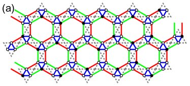
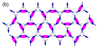
Figure 1: (a) Rydberg atoms arranged on a ruby lattice. White (black) dots correspond to atoms in the ground (excited) state. In this figure, $\langle n_{i}\rangle=1/4$. (b) Any state on the ruby lattice following the specification above can be mapped onto a dimer covering on the kagome lattice. Alternatively, it can also be represented in terms of a spin ice state, as indicated by the arrows.

Fractonic spin liquids (FSLs) form a distinct class of phases that can also be found in exactly solvable models and described by exotic quantum field theories [14]. FSLs are characterized by a robust subextensive ground state degeneracy and immobile excitations called fractons, which hinder thermal equilibrium at low temperatures [15]. In type-I FSLs, fractons can form composite excitations that are mobile only within a lattice submanifold. The restricted mobility of FSL excitations in real space is reflected on the corresponding field theories, which typically involve tensor gauge fields and dipole conservation laws [16, 17, 18, 19, 20, 21, 22, 23, 24, 25, 26, 27, 28, 29].

While fracton order is restricted to exist only in three dimensions [30, 31, 32], similar physics can emerge in lower dimensions in the form of subsystem protected topological order (SSPT) or spontaneous subsystem symmetry breaking phases (SSSB) [33, 34, 35, 36]. Such phases share many similarities with FSLs, such as a geometry-dependent ground state degeneracy and mobility restrictions of the excitations, but differ in the structure of entanglement. In fact, fracton-like behavior has even been identified in classical models constructed from classical spins and Ising variables in two dimensions [37, 38, 39, 40] or canonically conjugate variables with dynamics described by Hamilton’s equations [41]. Here we shall use the term classical fractons to refer to these models.

Quantum simulators based on Rydberg atom arrays [42] provide potential platforms for both QSLs and FSLs. Rydberg atoms trapped on the ruby lattice are already capable of simulating the RVB spin liquid on the kagome lattice [43]. Geometry ensures the isomorphism between excited Rydberg atoms (Fig. 1) and singlets that occupy kagome lattice bonds [43, 44]. The low-energy cold-atom states are univocally mapped onto kagome dimer coverings, which resonate among themselves under tunable transverse fields. The measurements are then compared with the expectation values predicted for a kagome quantum dimer model (KQDM), a projection of the usual Heisenberg model onto the covering set [45] that is also exactly solvable [46, 47]. Alternatively, the KQDM is translated into a honeycomb lattice model of exchange interactions among $S=3/2$ spins subject to longitudinal and transverse fields [44]. The zero-field model hosts a dimer liquid corresponding to an equal weight superposition of kagome dimer coverings. The transverse fields introduce electric, magnetic, or fermionic anyon fluctuations, which drive the dimer liquid to different types of QSLs. In particular, both the spin-1/2 KHM and the kagome RVB occur in this model, thus providing a unified framework for two paradigmatic liquid phases.

In this paper, we study the exchange-frustrated model formulated in Ref. [44] in the form of a (classical) spin-orbital Kitaev model (SOKM). This rewriting elucidates both local and nonlocal symmetries, allowing us to uncover the extensive ground state degeneracy associated with the kagome dimer liquid, as well as the exact partition function of the SOKM. Analyzing the nonlocal symmetries, we identify a mechanism to lift the ground state degeneracy leading to a subextensive zero-point entropy. We also discuss the classical fractons and other excitations with restricted mobility that arise in this model. Finally, we study the continuum limit of this classical fracton model using previously developed techniques for $\Gamma$-matrix models [24, 25], illuminating its conservation laws by analogy with Chern-Simons-like theories.

The paper is organized as follows. Section II presents several exact results on the SOKM, connecting the latter with the well-established physics of frustrated phases on the kagome lattice. In Sec. II.1, we review the theoretical models that describe quantum simulations of Rydberg atoms on the ruby lattice in the blockade limit with a fixed density of excited atoms [43, 44]. Section II.2 lists the SOKM symmetries which are then applied to determine its ground state manifold. This analysis automatically leads to classical analogues of Lieb’s theorem for gauge fluxes [48] and topological order in gapped $Z_{2}$ QSLs [49]. The symmetries also determine the level degeneracies, leading to a closed form for the partition function that recovers general features of spin ice thermodynamics [50, 51, 47, 52]. We use these results to compute the exact static structure factor in Section II.3, which presents the expected $Z_{2}$ spin ice character of the ground states. In Sec. III, we first introduce a sublattice-dependent rotation that maps the ferromagnetic and antiferromagnetic models and simplifies the notation in the remainder of the paper. We then construct a perturbation that does not commute with local plaquette operators but with strings in two distinct directions. This perturbation lifts the extensive zero-point entropy while also inducing classical fractons. We show that this model projected on the subspace of SOKM ground states is similar to the square-lattice fracton model studied in Ref. [37]. In Sec. IV, we construct an effective field theory for the SOKM. Using this framework, we recover the main features of the lattice model and relate the ground state degeneracy to the algebra of line operators defined in the continuum limit. Finally, we present our conclusions and outlook in Sec. V. The appendix contains explicit expressions for the matrix representations of spin-orbital operators used in this work.

II The Classical Spin-Orbital Kitaev Model

II.1 Equivalence between the Kagome Dimer Model and the Spin-orbital Kitaev model

We briefly review the minimal model for Rydberg atoms arranged on a ruby lattice [see Fig. 1(a)] as proposed in Ref. [44], both for completeness and to set the notation. Each atom is a hard-core boson located at a site $i$. We assign $n_{i}=0$ or $n_{i}=1$ if the atom is in the ground or excited Rydberg state, respectively. The Hamiltonian is given by [44]

$$H_{\text{diag}}=U\sum_{\langle ij\rangle_{\triangle}}n_{i}n_{j}+V\sum_{\langle ij\rangle_{\square}}n_{i}n_{j}-\delta\sum_{i}n_{i},$$ (1)

where $U$ ($V$) is the Rydberg blockade repulsion within (outside) the lattice triangles and $\delta$ is the laser detuning. Here, $\langle ij\rangle_{\triangle}$ corresponds to bonds on triangles and $\langle ij\rangle_{\square}$ on the ruby lattice rectangles. This Hamiltonian is readily converted into a classical Ising model via $n_{i}=\left(1+s_{i}^{z}\right)/2$. Quantum fluctuations can be induced by an external coherent laser with Rabi frequency $\Omega$ or by setting the simulator with cold atoms in two different dipole-coupled Rydberg states [42] leading to

$$H_{\text{fl}}=\Omega\sum_{i}s_{i}^{x}+U^{\prime}\sum_{\langle ij\rangle_{\triangle}}\left(s_{i}^{+}s_{j}^{-}+s_{i}^{-}s_{j}^{+}\right),$$ (2)

in which we neglected inter-triangle fluctuations. Hereafter we will assume the blockaded limit $U\rightarrow\infty$ and the average occupation number $\left\langle n_{i}\right\rangle=1/4$, a good approximation to actual quantum simulations [43].

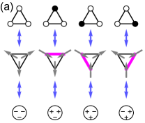
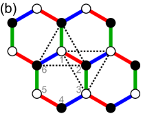
Figure 2: (a) Equivalence between spin-3/2 states labeled by $\left|a^{x},a^{y},a^{z}\right\rangle$ and ruby lattice states. (b) Section of the honeycomb lattice, in which $x$, $y$, and $z$ bonds are colored blue, red, and green, respectively. Here, black and white dots mark sites on the odd and even sublattices, respectively. A four-site star is formed by the sites on the corners of a dashed triangle plus the site at its center.

One ground state of $H_{\text{diag}}$ is illustrated in Fig. 1(a). The repulsion $U$ selects triangles with at most one Rydberg state, while $V$ tends to maximize the distance between two of these excitations. Since the ruby lattice is the medial lattice of the kagome [47], states that minimize the interaction energy of $H_{\text{diag}}$ in the sector $\left\langle n_{i}\right\rangle=1/4$ can be mapped to kagome dimer coverings; see Fig. 1(b). It is also possible to set a correspondence between dimer coverings and spin-ice states formed by triangles in two-in-one-out and three-out arrow configurations [45, 46, 47]; see Fig. 2. Counting arguments show that there are $2^{N+1}$ distinct dimer coverings on the kagome lattice [46, 47], in which $N$ is the number of unit cells, implying an extensive zero-point entropy. Quantum fluctuations in Eq. (2) introduce resonances among the coverings, allowing the simulation of RVB physics [43]. An exhaustive classification of anyon fluctuations was already performed in Ref. [44] and will not be repeated here, where we focus on the classical physics of $H_{\text{diag}}$.

The four allowed configurations in each triangle define spin-3/2 states placed on a honeycomb lattice. The associated observables are more conveniently written in terms of pseudospin ($\boldsymbol{\sigma}$) and pseudo-orbitals $(\boldsymbol{\tau})$ variables, each of them satisfying $\zeta^{x}\zeta^{y}\zeta^{z}=i$ ($\zeta=\sigma,\tau$) and the following algebra [53, 54, 55, 56, 57]:

$$\left\{\sigma_{i}^{\alpha},\sigma_{i}^{\beta}\right\} =\left\{\tau_{i}^{\alpha},\tau_{i}^{\beta}\right\}=2\delta^{\alpha\beta},$$

$$\left[\sigma_{i}^{\alpha},\sigma_{i}^{\beta}\right] =2i\delta_{ij}\epsilon^{\alpha\beta\gamma}\sigma_{i}^{\gamma},$$

$$\left[\tau_{i}^{\alpha},\tau_{i}^{\beta}\right] =2i\delta_{ij}\epsilon^{\alpha\beta\gamma}\tau_{i}^{\gamma},$$

$$\left[\sigma_{i}^{\alpha},\tau_{j}^{\beta}\right] =0.$$ (3)

Such operators have been discussed at length in the context of QSLs on Kugel-Khomskii models specially for the SU(4) Heisenberg model [53, 58, 59, 60] and exactly solvable extensions of the KHM [61, 62, 63, 64, 65, 55, 56, 57]. Crucially, the first and last relations in Eq. (3) imply that the operators

$$A_{i}^{\gamma}=\sigma_{i}^{\gamma}\tau_{i}^{\gamma}$$ (4)

commute among themselves. In conjunction with $A_{i}^{x}A_{i}^{y}A_{i}^{z}=-1$, this implies that they can be diagonalized as follows:

$$A^{x} =\text{diag}\left(-1,1,-1,1\right)=\left[a^{x}\right],$$

$$A^{y} =\text{diag}\left(-1,1,1,-1\right)=\left[a^{y}\right],$$

$$A^{z} =\text{diag}\left(-1,-1,1,1\right)=\left[a^{z}\right].$$ (5)

The representation of other spin-3/2 operators in this basis is explicitly provided in Appendix A. Throughout this paper, single-site states are labeled by $\left|a^{x},a^{y},a^{z}\right\rangle$ with $a^{\gamma}=\pm$ as indicated in Fig. 2(a). In terms of the spin-ice representation, $a^{\gamma}=+1$ ($a^{\gamma}=-1$) is equivalent to an incoming (outgoing) arrow on the triangle. When depicting the state on a site $i$ of the honeycomb lattice, we place the $a^{\gamma}$ closer to the $\gamma$ bond connected to the site, following Kitaev’s convention [7] shown in Fig. 2(b).

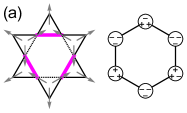
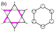
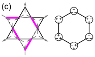
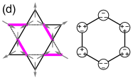
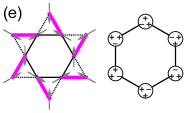
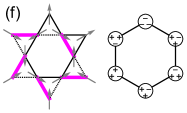
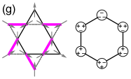
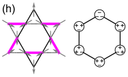
Figure 3: Equivalence between loop states on the kagome lattice, as studied in Refs. [45, 46, 47], and the present paper. All these states clearly satisfy $W^{A}_{p}=+1$, see Eq. (8), imposing a constraint on the outward $a^{\gamma}$ eigenvalues. All previously found loops can be obtained on the honeycomb representation by cyclic permutation around the plaquette and application of the operator $W_{p}^{\sigma}$ in Eq. (9).

The Hamiltonian $H_{\text{diag}}$ in the blockade limit and appropriate excitation density then reads [44]

$$H_{\text{diag}} =H_{\text{SOKM}}+H_{l},$$ (6)

where $H_{l}=h_{l}\sum_{i}\left(A_{i}^{x}+A_{i}^{y}+A_{i}^{z}\right)$ is a longitudinal field with $h_{l}=\left(V-\delta\right)/4$, which can be set to zero by varying the detuning, and $H_{\text{SOKM}}$ is the SOKM defined as

$$H_{\text{SOKM}} =J\sum_{\langle ij\rangle_{\gamma}}A_{i}^{\gamma}A_{j}^{\gamma},$$ (7)

in which $J=V/4>0$. In view of the bond-dependent anisotropic interactions, this model is a classical analogue of the KHM [7]. Figure 3 shows the states around an elementary hexagonal plaquette $p$ that minimize the interactions on all bonds. A unifying feature of these states is that the product of all outward $a^{\gamma}$ equals $+1$. More precisely, the ground state must be in the sector $W_{p}^{A}=+1$ $\forall p$, where

$$W_{p}^{A}=A_{1}^{z}A_{2}^{x}A_{3}^{y}A_{4}^{z}A_{5}^{x}A_{6}^{y},$$ (8)

in which the site labels follow Fig. 2(b). We refer to the subspace spanned by states with $W_{p}^{A}=+1$ $\forall p$ as the zero-flux sector, establishing a classical analogue of a theorem by Lieb [48] that fixes the ground state sector in the KHM [7]. The $2^{6}/2=32$ possibilities for the outward $\left\{a^{\gamma}\right\}$ correspond to the 32 loop configurations around hexagons on the kagome lattice [45], as illustrated in Fig. 3.

II.2 Symmetries, Exact Spectrum and Partition Function of the Spin-Orbital Kitaev Model

The main properties of the SOKM follow from its local symmetries. Assuming periodic boundary conditions, we can identify the ground state manifold starting from the reference ground state $\left|\phi_{0}\right\rangle$ shown in Fig. 4(a). In analogy to Eq. (8), we define the plaquette operators

$$W_{p}^{\sigma}=\sigma_{1}^{z}\sigma_{2}^{x}\sigma_{3}^{y}\sigma_{4}^{z}\sigma_{5}^{x}\sigma_{6}^{y}.$$ (9)

Such plaquette operators still commute with Eq. (7) while locally changing $\left|a^{x},a^{y},a^{z}\right\rangle$ of sites pertaining to $p$. This observation allows the construction of the following ground state family:

$$\left|\psi_{0}\left(\left\{S_{p}\right\}\right)\right\rangle=\prod_{p=1}^{N}\left(W_{p}^{\sigma}\right)^{S_{p}}\left|\phi_{0}\right\rangle,$$ (10)

in which $S_{p}=0,1$; see Fig. 4(b) for a minimal example. We could also define plaquette operators $W_{p}^{\tau}$ using the pseudo-orbital operators, but the relation $W_{p}^{\sigma}W_{p}^{\sigma}=W_{p}^{A}$ implies that the states generated by applying $W_{p}^{\tau}$ differ from Eq. (10) only by a global phase factor, thus being physically equivalent. The constraint $\prod_{p}W_{p}^{\sigma}=+1$ in the ground state sector implies that Eq. (10) provides $2^{N-1}$ ground states on a lattice with $N$ unit cells.

In addition to the local symmetries, the SOKM also commutes with nonlocal operators defined over noncontractible strings. Consider, for example,

$$V_{l_{xy}}^{\sigma}=\prod_{i\in l_{xy}}\sigma_{i}^{z},$$ (11)

which flips $\left\{a_{i}^{x}\right\}$ and $\left\{a_{i}^{y}\right\}$ along an $xy$ zigzag chain labeled by $l_{xy}$; see Fig. 4(c). A new ground state $\left|\Phi_{0}\right\rangle$ can be written as follows:

$$\left|\Phi_{0}\left(\left\{S_{l_{xy}}\right\}\right)\right\rangle=\prod_{l_{xy}=1}^{L_{xy}}\left(V_{l_{xy}}^{\sigma}\right)^{S_{l_{xy}}}\left|\phi_{0}\right\rangle,$$ (12)

in which $S_{l_{xy}}=0,1$ and $L_{xy}$ is the number of $xy$ chains. An even number of $V_{l_{xy}}^{\sigma}$ corresponds to the application of $W_{p}^{\sigma}$ operators around the honeycomb lattice following a set of $xy$ chains, but an odd number of $V_{l_{xy}}^{\sigma}$ cannot be generated using this operation. This even-odd distinction classifies the ground states by the parity of the string operators connecting it to the reference ground state $\left|\phi_{0}\right\rangle$. Since the lattice is two dimensional, we can repeat this discussion for another set of noncontractible loops, say, the ones along $yz$ chains labeled by $l_{yz}=1,\dots,L_{yz}$. As a consequence, the parity of the number of noncontractible strings on a torus defines $2^{2}=4$ ground state sectors, in each of which we can generate the states in Eq. (10). The resulting ground state degeneracy is $4\times 2^{N-1}=2^{N+1}$, for $N=L_{xy}L_{yz}$ unit cells. Clearly, this classical analogue of $Z_{2}$ topological degeneracy [49] is essential to recover the aforementioned degeneracy related to kagome dimer coverings [46, 47].

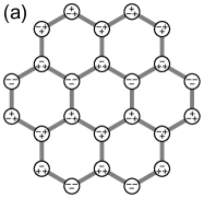
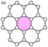
Figure 4: Illustration of the ground state and excitations of the spin-orbital Kitaev model in terms of eigenstates of $A_{i}^{\gamma}$. (a) Reference ground state $\left|\phi_{0}\right\rangle$ of the spin-orbital Kitaev model. (b) Ground state generated by a single plaquette operator, $W_{p}^{\sigma}\left|\phi_{0}\right\rangle$. (c) Ground state generated by a single string operator, $V_{l_{xy}}^{\sigma}\left|\phi_{0}\right\rangle$. (d) Single-flip excitation leading to two unsatisfied bonds and two $\pi$-flux plaquettes.

We can also use the symmetries to calculate the partition function of the SOKM. Figure 4(d) represents a minimally excited state of energy $4J$, obtained by applying a local operator $\sigma_{i}^{\gamma}$ on a ground state. This operator preserves the eigenvalue $a_{i}^{\gamma}$ while flipping the other two eigenvalues, $a_{i}^{\alpha},a_{i}^{\beta}$, thus changing the interaction energy on the $\alpha,\beta$ bonds. This excited state contains two visons [46, 47] associated with $W_{p}^{A}=-1$, equivalent to a $\pi$ flux through the plaquette. Note that visons are always created or annihilated in pairs. Hence, the spectrum reads

$$E_{n}=-3NJ+4nJ,\qquad n\geq 0.$$ (13)

Visons can be separated by arbitrary distances without an energy cost by applying $\sigma_{j}^{\gamma}$ along open strings. Combining the distinct ways of distributing the $2n$ unsatisfied bonds with the degeneracy arising from the symmetry operators, we obtain the degeneracy of each energy level:

$$g\left(E_{n}\right)=2^{N+1}\left(\begin{array}[]{c}3N\\ 2n\end{array}\right),$$ (14)

whose summation recovers the Hilbert space dimension. Using Eqs. (13) and (14), we obtain the partition function

$$Z = \sum_{n}g\left(E_{n}\right)e^{-\beta E_{n}}$$ (15)

$$= 2^{N}e^{3NJ\beta}\left[\left(1+e^{-2\beta J}\right)^{3N}+\left(1-e^{-2\beta J}\right)^{3N}\right].$$

The partition function allows us to compute the thermodynamics of the SOKM, which displays the qualitative behavior expected for spin ice [50, 51, 47, 52]. The free energy $F=-\frac{1}{\beta}\ln Z$ has the usual high-temperature limit given by

$$F\left(T\rightarrow\infty\right) =-3NJ-2Nk_{B}T\ln 4,$$ (16)

which recovers the expected entropy per site of $s_{\infty}=k_{B}\ln 4$. On the other hand, the low-temperature limit $T\rightarrow 0$ yields

$$F\left(T\rightarrow 0\right) =-3NJ-\left(N+1\right)k_{B}T\ln 2,$$ (17)

which reflects the $2^{N+1}$-fold ground state degeneracy and leads to an entropy per site of $s_{0}=\frac{1}{2}k_{B}\ln 2$ in the thermodynamic limit. Such residual entropy is a defining characteristic of spin ice systems and can be experimentally estimated using specific heat integration [50, 51, 47, 52]. From the exact partition function, we can also calculate the specific heat and entropy per site at arbitrary temperatures. The result is shown in Fig. 5(a), where the dashed lines highlight the low- and high-temperature limits. Notice that the SOKM does not exhibit a phase transition but rather a crossover connecting the spin-ice and the paramagnetic regimes.

II.3 Static Structure Factor

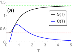
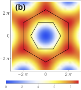
Figure 5: (a) Entropy $S(T)$ and specific heat $C(T)$ per site of the spin-orbital Kitaev model (in units of $k_{B}$) as a function of temperature in units of $J/k_{B}$. The dotted line indicates the zero-point entropy of $\frac{1}{2}\ln 2$, while the dashed line corresponds to the high-temperature entropy of $\ln 4$. (b) Static structure factor of the spin-orbital Kitaev model. The smaller hexagon corresponds to the boundaries of the first Brillouin zone, while the larger plaquette connects neighboring spectral weight maxima.

We now turn to the calculation of the static structure factor

$$S\left(\mathbf{q},T\right)=\frac{1}{N}\text{Tr}\left[\hat{\rho}\left(T\right)\sum_{\alpha,\beta}\sum_{i,j}A_{i}^{\alpha}A_{j}^{\beta}e^{i\mathbf{q}\cdot\left(\mathbf{r}_{i}-\mathbf{r}_{j}\right)}\right],$$ (18)

in which $\hat{\rho}$ is the density matrix. We are particularly interested in the low-temperature limit, where the correlation function simplifies to

$$\lim_{T\rightarrow 0}S\left(\mathbf{q},T\right)=\sum_{\underset{i,j}{\psi_{0},\alpha,\beta,}}\frac{\left\langle\psi_{0}\left|A_{i}^{\alpha}A_{j}^{\beta}\right|\psi_{0}\right\rangle}{2^{N+1}N}e^{i\mathbf{q}\cdot\left(\mathbf{r}_{i}-\mathbf{r}_{j}\right)},$$ (19)

in which $\psi_{0}$ runs over the ground state manifold. It is then convenient to define

$$\left|0\right\rangle\equiv\frac{1}{\sqrt{2^{N+1}}}\sum_{\psi_{0}}\left|\psi_{0}\right\rangle.$$ (20)

Since

$$A_{i}^{\alpha}A_{j}^{\beta}\left|\psi_{0}\right\rangle =a_{i}^{\alpha}a_{j}^{\beta}\left|\psi_{0}\right\rangle,\,a_{i}^{\alpha},a_{j}^{\beta}=\pm 1,$$

$$\left\langle\psi_{0}^{\prime}|\psi_{0}\right\rangle =\delta_{\psi_{0}^{\prime},\psi_{0}},$$ (21)

we can write the $T\rightarrow 0$ correlation as

$$S\left(\mathbf{q}\right)=\frac{1}{N}\sum_{\underset{i,j}{\alpha,\beta,}}\left\langle 0\left|A_{i}^{\alpha}A_{j}^{\beta}\right|0\right\rangle e^{i\mathbf{q}\cdot\left(\mathbf{r}_{i}-\mathbf{r}_{j}\right)}.$$ (22)

The $\left|0\right\rangle$ state is the honeycomb representation of the kagome dimer liquid discussed in Refs. [46, 47], which allows us to assert the ultrashort correlation functions

$$\left\langle 0\left|A_{i}^{\alpha}A_{j}^{\beta}\right|0\right\rangle=\delta^{\alpha\beta}\times\begin{cases}1,&\text{if }i=j,\\ -1,&\text{if }i,j\in\left\langle ij\right\rangle_{\alpha}\\ 0,&\text{otherwise}.\end{cases}$$ (23)

The first two equations are explained by the antiferromagnetic Ising couplings of $Z_{2}$ local states. On the kagome lattice, the last equation reflects the independence of dimer states for triangles that do not share a vertex. This is the classical analogue of the KHM correlation function, which is known to vanish beyond nearest neighbors from analytical arguments [66, 67]. Substituting Eq. (23) in Eq. (22), we find

$$S\left(\mathbf{q}\right) =4\sum_{\gamma}\sin^{2}\left(\frac{\mathbf{q}\cdot\boldsymbol{\delta}_{\gamma}}{2}\right),$$ (24)

where $\boldsymbol{\delta}_{z}=\frac{\sqrt{3}}{3}\left(0,-1\right)$, $\boldsymbol{\delta}_{x,y}=\frac{\sqrt{3}}{3}\left(\pm\frac{\sqrt{3}}{2},\frac{1}{2}\right)$ are the nearest-neighbor vectors of the honeycomb lattice.

The structure factor $S\left(\mathbf{q}\right)$ plotted in Fig. 5(b) displays no signature of conventional long-range order, as expected from a classical spin liquid. The momentum dependence is commensurate with the lattice periodicity and consistent with the $Z_{3}$ rotational invariance of the model. The correlations are weak in the neighborhood of the $\Gamma$ point, remaining relatively small for all points inside the first Brillouin zone. The spectral weight is maximal at some reciprocal lattice points and remains large along the edges connecting them. Such a pattern is reminiscent of the spin ice structure factor, with the key difference that there are no pinch point singularities in the SOKM due to the ultrashort correlations.

III Classical Fractons

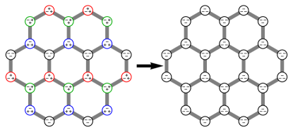
Figure 6: Illustration of the Klein-like transformation applied to the reference ground state. We perform a $\pi$ rotation around the $\sigma^{z}$ axis on blue sites, $\sigma^{x}$ on red sites, and $\sigma^{y}$ on green sites. This transformation effectively invert the sign of the exchange coupling, leading to the ferromagnetic model in Eq. (25).

We are now ready to study how to lift the local symmetries associated with $W_{p}^{\sigma}$ while retaining string symmetries $V_{l}^{\sigma}$ in a manner that induces fracton excitations. To simplify the onward discussion, we will work on a rotated frame characterized by a site-dependent pseudospin rotation $A_{j}^{\gamma}\rightarrow e^{i\pi\sigma_{j}^{\alpha}/2}A_{j}^{\gamma}e^{-i\pi\sigma_{j}^{\alpha}/2}$, with the rotation axis chosen locally as indicated in Fig. 6. In this frame, the reference ground state $\left|\phi_{0}\right\rangle$ is transformed into a “ferromagnetic” reference state based on $\left|a^{x},a^{y},a^{z}\right\rangle=\left|-,-,-\right\rangle$. More generally, this sublattice-dependent rotation is akin to a Klein transformation in the Kitaev-Heisenberg model [68, 69, 70] that effectively inverts the sign of the exchange coupling:

$$H_{\text{SOKM}}=-J\sum_{\left\langle ij\right\rangle_{\gamma}}A_{i}^{\gamma}A_{j}^{\gamma}.$$ (25)

We stress that the symmetries detailed in the previous section remain valid for the ferromagnetic model. Within this description, the next figures can be unburdened from many sign factors by no longer displaying the $\left|-,-,-\right\rangle$ state. We will also denote the other local states by

$$\left|x\right\rangle \equiv\left|-,+,+\right\rangle,$$

$$\left|y\right\rangle \equiv\left|+,-,+\right\rangle,$$

$$\left|z\right\rangle \equiv\left|+,+,-\right\rangle.$$ (26)

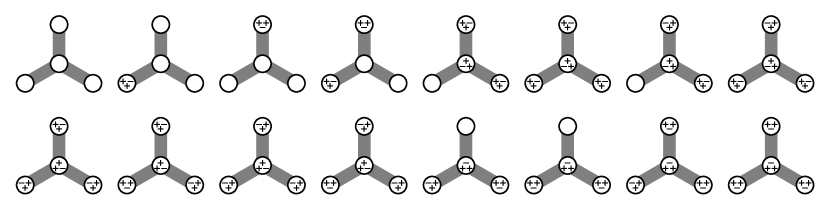
Figure 7: States $\left|\psi\left(i,i_{x},i_{y},i_{z}\right)\right\rangle$ with $i$ on the even sublattice that satisfy $P^{\prime}_{i}\left|\psi\left(i,i_{x},i_{y},i_{z}\right)\right\rangle=\left|\psi\left(i,i_{x},i_{y},i_{z}\right)\right\rangle$. For all other four-site states $\left|\phi\right\rangle$, $P^{\prime}_{i}\left|\phi\right\rangle=0$. Projected states for the stars centered on odd sublattices are obtained by inversion. Empty circles represent $\left|a^{x},a^{y},a^{z}\right\rangle=\left|-,-,-\right\rangle$.

Any perturbation that commutes with string operators such as those in Eq. (12) but not with the plaquette operators $W_{p}^{\sigma}$ lifts the ground state degeneracy. As a warm-up example, we consider the longitudinal field

$$H_{\text{ext}}=h\sum_{i}A_{i}^{z}.$$ (27)

This perturbation quantifies laser tuning effects that localize Rydberg excitations along predefined lines, an experimentally feasible setup [71]. Such a field commutes with $V_{l_{xy}}^{\sigma}$ but not with $W_{p}^{\sigma}$ or $V_{l_{yz}}^{\sigma}$ and $V_{l_{xz}}^{\sigma}$, immediately implying that the model $H_{\text{SOKM}}+H_{\text{ext}}$ has its degeneracy lifted to $2^{L_{xy}}$. Excitations can be created on $x$ and $y$ bonds [see Fig. 4(d)] and then separated without energy penalty if they are kept along the $xy$ chain. The same excitations do not propagate along the transverse direction, implying that the model now hosts excitations with restricted mobility (or lineons). However, $H_{\text{ext}}$ does not induce immobile excitations, which is thus insufficient to introduce fracton physics.

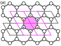
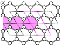
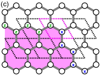
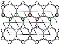
Figure 8: Excited states of the fracton model in Eq. (30) on the zero-flux sector. Magenta hexagons represent plaquettes where the $W_{p}^{\sigma}$ operator was applied in relation to the reference ground state. (a) The excited state generated by a single $W_{p}^{\sigma}$. In the dual-lattice description, it frustrates the four rhomboids touching the central plaquette. (b) Lineon excitation generated from the application of $W_{p}^{\sigma}$ over a line of plaquettes leading to two unsatisfied rhomboids. (c) Classical fracton with a single unsatisfied rhomboid. (d) Effect of the four-dimensional local Hilbert space in terms of string operator intersections. (e) Representation of the classical fracton on the dual lattice. We emphasize that a given state in this dual representation can be represented in different ways.

Immobile excitations arise once we introduce a perturbation commuting with strings in two different directions. To construct an operator with the desired property, consider the $\left|\phi_{0}\right\rangle$ state as well as other states obtained by the action of $V_{l_{xy}}^{\sigma},V_{l_{yz}}^{\sigma}$ strings. In all these states, the four-site stars centered at a given site $i$ have 16 different possibilities, all of which are indicated in Fig. 7 (apart from the inversion symmetry leading to four-site states centered on the other sublattice). Let $P_{i}^{\prime}$ be the four-site projection operator satisfying $P_{i}^{\prime}\left|\xi_{i}\right\rangle=\left|\xi_{i}\right\rangle$, if $\left|\xi_{i}\right\rangle$ is one of the states in Fig. 7, and $P_{i}^{\prime}\left|\xi_{i}\right\rangle=0$ otherwise. In terms of $A_{i}^{\alpha}$ operators, we have

$$P_{i}^{\prime} =\frac{1}{16}+\frac{1}{16}\left(A_{i}^{x}A_{i_{x}}^{x}+A_{i}^{y}A_{i_{y}}^{y}+A_{i}^{z}A_{i_{z}}^{z}\right)$$

$$+\frac{1}{16}\left(A_{i}^{x}A_{i_{y}}^{x}+A_{i_{x}}^{x}A_{i_{y}}^{x}+A_{i}^{z}A_{i_{y}}^{z}+A_{i_{y}}^{z}A_{i_{z}}^{z}\right)$$

$$-\frac{1}{16}\left(A_{i}^{x}A_{i_{y}}^{y}A_{i_{z}}^{z}+A_{i_{y}}^{x}A_{i}^{y}A_{i_{z}}^{z}+A_{i_{x}}^{x}A_{i}^{y}A_{i_{y}}^{z}+\right.$$

$$\left.+A_{i_{x}}^{x}A_{i_{y}}^{y}A_{i}^{z}+A_{i_{x}}^{x}A_{i}^{y}A_{i_{z}}^{z}+A_{i_{x}}^{x}A_{i_{y}}^{y}A_{i_{z}}^{z}\right)$$

$$+\frac{1}{16}\left(A_{i}^{x}A_{i_{x}}^{x}A_{i_{y}}^{z}A_{i_{z}}^{z}+A_{i_{x}}^{x}A_{i_{y}}^{x}A_{i}^{z}A_{i_{z}}^{z}\right),$$ (28)

in which $i$ is the site at the center of the star and $i_{\gamma}$ is the neighboring site along the $\gamma$ bond. Such a projector commutes with $V_{l_{xy}}^{\sigma}$ and $V_{l_{yz}}^{\sigma}$ by construction. It is also clear from the first line of Eq. (28) that some of its terms commute with all $W_{p}^{\sigma}$. Let us then consider two neighboring stars, one centered on the even and other on the odd sublattice, as depicted in Fig. 2(b). The interactions in $P_{i}^{\prime}$ that simultaneously anticommute with $W_{p}^{\sigma}$ for all four plaquettes shown in Fig. 2(b) are

$$P_{i} =\frac{1}{16}\left(A_{i}^{x}A_{i_{y}}^{x}+A_{i_{x}}^{x}A_{i_{y}}^{x}+A_{i}^{z}A_{i_{y}}^{z}+A_{i_{y}}^{z}A_{i_{z}}^{z}\right)$$

$$-\frac{1}{16}\left(A_{i_{y}}^{x}A_{i}^{y}A_{i_{z}}^{z}+A_{i_{x}}^{x}A_{i}^{y}A_{i_{y}}^{z}\right)$$

$$+\frac{1}{16}\left(A_{i}^{x}A_{i_{x}}^{x}A_{i_{y}}^{z}A_{i_{z}}^{z}+A_{i_{x}}^{x}A_{i_{y}}^{x}A_{i}^{z}A_{i_{z}}^{z}\right).$$ (29)

We then define the classical fracton model as follows:

$$H=-J\sum_{\left\langle ij\right\rangle_{\gamma}}A_{i}^{\gamma}A_{j}^{\gamma}-\lambda\sum_{i}P_{i}.$$ (30)

A simplified minimal model can be obtained in the zero-flux sector considering the dual lattice formed by the centers of the hexagons. Let the dual-lattice states be distinguished by how many times the $W_{p}^{\sigma}$ operators are applied over the reference state $\left|\phi_{0}\right\rangle$. Inserting one $W_{p}^{\sigma}$ as illustrated in Fig. 8(a) generates excitations on eight stars centered on the sites located inside the highlighted rhomboids. We can reduce the number of excitations by four stars if a semi-infinite line of excitations is inserted, as indicated in Fig. 8(b). Note that the pair of $x,y$ states at the end of the line in Fig. 8(b) can move as a lineon. The minimum number of excitations in the vicinity of the original plaquette is obtained after applying $W_{p}^{\sigma}$ as illustrated in Fig. 8(c). This operation defines extended membrane operators, whose edges run along the directions of $xy$ and $yz$ chains. The isolated excitations live at the corners of the membrane and cannot be moved without creating additional excitations. This behavior is captured by the effective model

$$H_{\text{eff}}=-J\sum_{\langle ijkl\rangle}\mathcal{Y}_{i}\mathcal{Y}_{j}\mathcal{Y}_{k}\mathcal{Y}_{l},$$ (31)

in which $i,j,k,l$ are sites on the dual lattice and $\mathcal{Y}_{i}=-1$ if there is a plaquette operator inserted on this site, otherwise, $\mathcal{Y}_{i}=1$.

The Hamiltonian in Eq. (31) is remarkably similar to the square-lattice model studied in Ref. [37], in the sense that the interaction is a product of four Ising variables defined at the center of four plaquettes. In fact, it can be understood as an SSSB phase, similar to that of the Xu-Moore model [72, 73] (or plaquette Ising model [34]). A key difference concerns the ground state degeneracy, which is equivalent to $2^{L_{xy}+L_{yz}-1}$ in Ref. [37], whereas it is $2^{L_{xy}+L_{yz}}$ in the present model. The root of this difference lies in the four-dimensional Hilbert space at each site, which implies that at the intersection of $V_{l_{xy}}^{\sigma}$ and $V_{l_{yz}}^{\sigma}$ we do not find $\left\rceil-,-,-\right\rangle$ states, but rather the $y$ state; see Fig. 8(d). We can account for this difference by treating $\mathcal{Y}_{i}$ as a four-state operator just like $A_{i}^{\gamma}$. Using the ordered basis $\left\{\left|0\right\rangle,\left|X\right\rangle,\left|Y\right\rangle,\left|Z\right\rangle\right\}$, we write

$$\mathcal{Y}=\text{diag}\left(+,-,+,-\right).$$ (32)

The $\left|0\right\rangle$ state corresponds to the absence of $W_{p}^{\sigma}$, while an isolated $\left|X\right\rangle$ ($\left|Z\right\rangle$) state corresponds to the combination of two lineons limited by $yz$ ($xy$) chains. The $\left|Y\right\rangle$ state corresponds to the absence of $W_{p}^{\sigma}$ due to the intersection between $\left|X\right\rangle$ and $\left|Z\right\rangle$ at a given point of the dual lattice. All zero-flux states satisfying the bond energy can be mapped onto a state on the dual lattice, as exemplified by the fracton state in Fig. 8(e).

IV Effective field theory

In this section we construct and analyze an effective field theory that captures the main properties of the lattice model, notably the existence of conserved line operators and the associated ground state degeneracy.

We start by rewriting the SOKM Hamiltonian as

$$H_{\rm SOKM}=-J\sum_{\gamma}\sum_{\mathbf{R}_{\gamma}}O({\mathbf{R}_{\gamma}}),$$ (33)

where $\mathbf{R}_{\gamma}$ are the positions of the centers of the $\gamma$ bonds and $O(\mathbf{R}_{\gamma})=A^{\gamma}(\mathbf{R}_{\gamma}+\frac{1}{2}\boldsymbol{\delta}_{\gamma})A^{\gamma}(\mathbf{R}_{\gamma}-\frac{1}{2}\boldsymbol{\delta}_{\gamma})$. Here we use the notation $A_{j}^{\gamma}=A^{\gamma}(\mathbf{r}_{j})$ for the operators that act on site $j$, at position $\mathbf{r}_{j}$ in the honeycomb lattice. For fixed $\gamma$, the set $\{\mathbf{R}_{\gamma}\}$ forms a triangular lattice. Crucially, $O(\mathbf{R}_{\gamma})$ are mutually commuting operators that square to the identity. Thus, the SOKM belongs to the class of frustration-free models whose ground state subspace is a stabilizer code. This property is required to apply the procedure described in Refs. [24, 26], as we shall do in the following. The first step is to introduce a new basis of operators:

$$\Gamma^{1}=\sigma^{x}\tau^{x},\;\Gamma^{2}=\sigma^{y}\tau^{x},\;\Gamma^{3}=\sigma^{z}\tau^{x},\;\Gamma^{4}=\sigma^{0}\tau^{y},$$ (34)

where $\sigma^{0}$ denotes the identity matrix in pseudospin space. We also define $\Gamma^{5}=\Gamma^{1}\Gamma^{2}\Gamma^{3}\Gamma^{4}$. These operators obey $\{\Gamma^{I},\Gamma^{J}\}=2\delta_{IJ}$ for $I,J\in\{1,\dots,5\}$. The operators $A^{\gamma}$ can be written as

$$A^{x}=\Gamma^{1},\quad A^{y}=i\Gamma^{1}\Gamma^{3}\Gamma^{4},\quad A^{z}=-i\Gamma^{3}\Gamma^{4}.$$ (35)

Next, we represent the operators $\Gamma^{I}$ using four bosonic fields. At each site, we introduce the fields $\theta_{n}(\mathbf{r}_{j})$, with $n\in\{1,\dots,4\}$, which obey the commutation relation

$$[\theta_{m}(\mathbf{r}),\theta_{n}(\mathbf{r}^{\prime})]=i\pi\delta_{\mathbf{r}\mathbf{r}^{\prime}}(K^{-1})_{mn},$$ (36)

where $K$ is the antisymmetric matrix

$$K=\left(\begin{array}[]{cccc}0&1&1&1\\ -1&0&1&1\\ -1&-1&0&1\\ -1&-1&-1&0\end{array}\right).$$ (37)

Following Refs. [24, 26], we use the “bosonization” map

$$\Gamma^{I}_{j}\sim\exp[it^{I}_{m}K_{mn}\theta_{n}(\mathbf{r}_{j})],$$ (38)

with an implicit sum over repeated indices $m,n\in\{1,\dots,4\}$. The vectors $t^{I}_{m}$ are chosen so that

$$t^{I}_{m}K_{mn}t^{J}_{n}=\begin{cases}0\text{ (mod 2)},\leavevmode\nobreak\ \leavevmode\nobreak\ \leavevmode\nobreak\ \text{if}\leavevmode\nobreak\ \leavevmode\nobreak\ \leavevmode\nobreak\ I=J,\\ 1\text{ (mod 2)},\leavevmode\nobreak\ \leavevmode\nobreak\ \leavevmode\nobreak\ \text{if}\leavevmode\nobreak\ \leavevmode\nobreak\ \leavevmode\nobreak\ I\neq J,\end{cases}$$ (39)

and $\sum_{I=1}^{5}t_{m}^{I}=0$. A convenient choice is

$$t_{m}^{I} = \delta_{Im},\quad\text{for }I=1,\dots,3,$$

$$t^{4}_{m} = -\delta_{m4}.$$ (40)

We write the local operators of the SOKM as

$$A^{\gamma}_{j}\sim\cos[\theta^{\gamma}(\mathbf{r}_{j})],$$ (41)

where $\theta^{\gamma}(\mathbf{r})=v_{m}^{\gamma}K_{mn}\theta_{n}(\mathbf{r})$, with

$$v_{m}^{x} = t_{m}^{1},$$

$$v_{m}^{y} = -t_{m}^{1}+t_{m}^{3}+t_{m}^{4},$$

$$v_{m}^{z} = -t_{m}^{3}-t_{m}^{4}.$$ (42)

The four-component vectors $v_{n}^{\gamma}$ are linearly dependent and satisfy

$$v^{\gamma}_{n}K_{mn}v^{\gamma^{\prime}}_{n}=0.$$ (43)

We then have $[\theta^{\gamma}(\mathbf{r}),\theta^{\gamma^{\prime}}(\mathbf{r}^{\prime})]=0$, which ensures the commutation of the physical operators $A^{\gamma}(\mathbf{r})$.

In the bosonic representation, the SOKM becomes

$$H_{\rm SOKM} = -\frac{J}{2}\sum_{\gamma}\sum_{\mathbf{R}_{\gamma}}\cos[2\theta^{\gamma}(\mathbf{R}_{\gamma})]$$ (44)

$$-\frac{J}{2}\sum_{\gamma}\sum_{\mathbf{R}_{\gamma}}\cos[\Delta_{\gamma}\theta^{\gamma}(\mathbf{R}_{\gamma})],$$

where

$$\theta^{\gamma}(\mathbf{R}_{\gamma}) = \frac{\theta^{\gamma}_{\rm e}(\mathbf{R}_{\gamma}+\boldsymbol{\delta}_{\gamma}/2)+\theta^{\gamma}_{\rm o}(\mathbf{R}_{\gamma}-\boldsymbol{\delta}_{\gamma}/2)}{2},$$ (45)

$$\Delta_{\gamma}\theta^{\gamma}(\mathbf{R}_{\gamma}) = \theta^{\gamma}_{\rm e}(\mathbf{R}_{\gamma}+\boldsymbol{\delta}_{\gamma}/2)-\theta^{\gamma}_{\rm o}(\mathbf{R}_{\gamma}-\boldsymbol{\delta}_{\gamma}/2).$$ (46)

Here we have added the subindex e,o to indicate that the that fields act on positions that belong to the even or odd sublattices of the honeycomb lattice, respectively. Assuming that we can take the continuum limit with fields that vary smoothly on the lattice scale, we replace $\Delta_{\gamma}\theta^{\gamma}\to\frac{1}{\sqrt{3}}a_{0}\partial_{\gamma}\theta^{\gamma}(\mathbf{r})$, where $a_{0}$ is the lattice spacing (set to $a_{0}=1$ in previous sections) and $\partial_{\gamma}=\hat{\boldsymbol{\delta}}_{\gamma}\cdot\nabla$ are spatial derivatives in the direction of the unit vectors $\hat{\boldsymbol{\delta}}_{\gamma}=\sqrt{3}\boldsymbol{\delta}_{\gamma}/a_{0}$. Expanding the second term in Eq. (44) to leading order in the derivatives, we obtain the effective Hamiltonian in the continuum limit

$$H_{\rm c}=\sum_{\gamma}\int d^{2}r\,\left[\frac{u}{2}(\partial_{\gamma}\theta^{\gamma})^{2}-g\cos(2\theta^{\gamma})\right],$$ (47)

where $u\sim J$ and $g\sim J/a_{0}^{2}$. This Hamiltonian respects the $Z_{3}$ symmetry that takes $\gamma\mapsto\gamma+1$ (mod 3) in real and internal space. The cosine term imposes the constraint that the physical values of the phase fields are $\theta^{\gamma}=0,\pi$ (mod $2\pi$), corresponding to the eigenvalues $a^{\gamma}=\pm 1$ of $A^{\gamma}$. If this term is irrelevant, we can treat $\theta^{\gamma}$ as continuous functions and focus on the effects of the first term in Eq. (47).

We can reformulate the effective field theory as a gauge theory. Let us consider the effective action

$$S=\int_{\mathcal{M}}d^{3}x\,\left(\frac{K_{mn}}{4\pi}\mathcal{A}_{m}\partial_{t}\mathcal{A}_{n}-\frac{1}{2\pi}\sum_{\gamma}\mathcal{A}_{0}^{\gamma}\partial_{\gamma}\mathcal{A}^{\gamma}\right),$$ (48)

where $\mathcal{M}$ is a spacetime manifold, $\mathcal{A}_{n}(\mathbf{r})=\theta_{n}(\mathbf{r})/a_{0}$ are rescaled fields with dimension of inverse length, with the linear combinations $\mathcal{A}^{\gamma}(\mathbf{r})=v_{m}^{\gamma}K_{mn}\mathcal{A}_{n}(\mathbf{r})$, and $\mathcal{A}_{0}^{\gamma}$ are Lagrange multipliers enforcing the constraint $\partial_{\gamma}\mathcal{A}^{\gamma}=0$ in the ground state subspace. This action is reminiscent of the Chern-Simons-like theories studied in Refs. [24, 25, 26, 28]. In fact, using Eq. (43) we verify that the action is invariant under the U(1) gauge transformation

$$\mathcal{A}_{m} \mapsto \mathcal{A}_{m}+\sum_{\gamma}v_{m}^{\gamma}\,\partial_{\gamma}G^{\gamma},$$ (49)

$$\mathcal{A}_{0}^{\gamma} \mapsto \mathcal{A}_{0}^{\gamma}+\partial_{t}G^{\gamma},$$ (50)

where $G^{\gamma}(\mathbf{r},t)$ are arbitrary dimensionless functions. Explicitly, the gauge transformation acts on the fields as

$$\mathcal{A}_{1} \mapsto \mathcal{A}_{1}+\partial_{1}G^{x}-\partial_{2}G^{y},$$ (51)

$$\mathcal{A}_{2} \mapsto \mathcal{A}_{2},$$ (52)

$$\mathcal{A}_{3} \mapsto \mathcal{A}_{3}+\partial_{2}G^{y}-\partial_{3}G^{z},$$ (53)

$$\mathcal{A}_{4} \mapsto \mathcal{A}_{4}-\partial_{2}G^{y}+\partial_{3}G^{z}.$$ (54)

Defining the linear combinations $\mathcal{A}_{\pm}=(\mathcal{A}_{3}\pm\mathcal{A}_{4})/2$, we note that $\mathcal{A}_{2}$ and $\mathcal{A}_{+}$ are gauge invariant. In order for $e^{i\mathcal{A}_{n}(\mathbf{r})}$ to describe physical operators for all components $\mathcal{A}_{n}$, the gauge functions must be restricted to the form

$$G^{\gamma}(\mathbf{r})=2\pi n^{\gamma}(\bar{x}_{\gamma})\,x_{\gamma}+f^{\gamma}(\bar{x}_{\gamma}),$$ (55)

where $x_{\gamma}=\mathbf{r}\cdot\hat{\boldsymbol{\delta}}_{\gamma}$ is the coordinate in the direction parallel to the $\gamma$ bond, $\bar{x}_{\gamma}$ is the coordinate in the perpendicular direction, $n^{\gamma}(\bar{x}_{\gamma})$ are integer functions, and $f^{\gamma}(\bar{x}_{\gamma})$ are arbitrary real functions. This type of behavior is common in higher-rank gauge theories, where it stems from the structure of higher derivatives and allows for discontinuous configurations in the low-energy sector [22, 74, 20, 75].

The equations of motion derived from the action in Eq. (48) lead to the conditions of vanishing “electric” and “magnetic” fields:

$$\mathcal{E}_{n} \equiv \partial_{t}\mathcal{A}_{n}-\sum_{\gamma}v_{n}^{\gamma}\partial_{\gamma}\mathcal{A}_{0}^{\gamma}=0,$$ (56)

$$\mathcal{B}^{\gamma} \equiv K_{mn}D^{\gamma}_{m}\mathcal{A}_{n}=0,$$ (57)

where $D^{\gamma}_{m}=v_{m}^{\gamma}\partial_{\gamma}$. From Eq. (56), we obtain

$$\partial_{t}\mathcal{A}_{2} = \partial_{t}\mathcal{A}_{+}=0,$$

$$\partial_{t}\mathcal{A}_{1} = \partial_{1}\mathcal{A}_{0}^{x}-\partial_{2}\mathcal{A}_{0}^{y},$$

$$\partial_{t}\mathcal{A}_{-} = \partial_{2}\mathcal{A}_{0}^{y}-\partial_{3}\mathcal{A}_{0}^{z}.$$ (58)

The conservation of $\mathcal{A}_{2}(\mathbf{r})$ and $\mathcal{A}_{+}(\mathbf{r})$ has a simple physical interpretation. In this classical theory, the Hamiltonian is a function of the mutually commuting fields $\theta^{\gamma}(\mathbf{r})$. These fields are linearly dependent and can be written in terms of only two independent components. For the parametrization in Eqs. (40) and (42), we have $\theta^{x}=\theta_{2}+2\theta_{+}$, $\theta^{y}=-\theta_{2}$, and $\theta^{z}=-2\theta_{+}$. Thus, the conservation of $\theta^{\gamma}$ implies that $\mathcal{A}_{2}$ and $\mathcal{A}_{+}$ become conserved quantities in the gauge theory.

The theory also contains local operators that involve the fields $\theta_{1}$ and $\theta_{-}=(\theta_{3}-\theta_{4})/2$ and act nontrivially on the eigenvalues of $A^{\gamma}\sim\cos(\theta^{\gamma})$. For instance, we have

$$\sigma_{j}^{z}=-i\Gamma^{1}_{j}\Gamma^{2}_{j}\sim e^{-i\theta_{1}},$$ (59)

where we omit the factors that depend on $\theta_{2}$ and $\theta_{+}$, which only give unimportant phases when acting on a ground state. The operator $e^{-i\theta_{1}}$ anticommutes with $\cos(\theta^{x,y})$ on the same site, but commutes with $\cos(\theta^{z})$. We can also check that $e^{-i\theta_{1}}$ commutes with the terms $\cos(2\theta^{\gamma})$ in the effective Hamiltonian in Eq. (47). Similarly, $\sigma_{j}^{x}\sim e^{-i(2\theta_{1}+\theta_{-})}$ anticommutes with $\cos(\theta^{y,z})$, but commutes with $\cos(\theta^{x})$.

We can now identify the line operators in the effective field theory. Consider the model defined on a torus with $L_{yz}$ unit cells in the direction of $\hat{\mathbf{e}}_{1}=\hat{\mathbf{x}}$ and $L_{xy}$ unit cells in the direction of $\hat{\mathbf{e}}_{2}=-\frac{1}{2}\hat{\mathbf{x}}+\frac{\sqrt{3}}{2}\hat{\mathbf{y}}$. Note that $\mathbf{r}\cdot\hat{\mathbf{e}}_{1}=\bar{x}_{3}$ and $\mathbf{r}\cdot\hat{\mathbf{e}}_{2}=\bar{x}_{1}$. The line operator associated with applying $\sigma_{j}^{z}$ along an $xy$ chain that winds around the torus has the form

$$V^{\sigma}_{l_{xy}}\sim\prod_{k=0}^{L_{yz}-1}e^{-i\theta_{1}(\mathbf{r}+ka_{0}\hat{\mathbf{e}}_{1})}e^{-i\theta_{1}(\mathbf{r}+\boldsymbol{\delta}_{1}+ka_{0}\hat{\mathbf{e}}_{1})},$$ (60)

where $\mathbf{r}$ belongs to the odd sublattice. Note that each line in the direction of $\hat{\mathbf{e}}_{1}$ has length $\ell_{1}=L_{yz}a_{0}$ and can be labeled by $(\mathbf{r}+ka_{0}\hat{\mathbf{e}}_{1})\cdot\hat{\boldsymbol{\delta}}_{3}=x_{3}$. Thus, in the continuum limit,

$$V^{\sigma}_{l_{xy}}\to\mathcal{V}_{z}(x_{3})\sim e^{-i\oint d\bar{x}_{3}(\mathcal{A}_{1}^{\rm o}+\mathcal{A}_{1}^{\rm e})}.$$ (61)

Here we have restored the indices $\nu=\text{e},\text{o}$ for even and odd sublattices, with the convention $\mathcal{A}_{n}=(\mathcal{A}_{n}^{\rm o}+\mathcal{A}_{n}^{\rm e})/2$. Similarly, the line operator acting on a $yz$ line with length $\ell_{2}=L_{xy}a_{0}$ is given in the continuum limit by

$$V^{\sigma}_{l_{yz}}\to\mathcal{V}_{x}(x_{1})\sim e^{-i\oint d\bar{x}_{1}(2\mathcal{A}_{1}^{\rm o}+2\mathcal{A}_{1}^{\rm e}+\mathcal{A}_{-}^{\rm o}+\mathcal{A}_{-}^{\rm e})}.$$ (62)

Using the commutation relation

$$[\mathcal{A}^{\nu}_{m}(\mathbf{r}),\mathcal{A}_{n}^{\nu^{\prime}}(\mathbf{r}^{\prime})]=i\delta_{\nu\nu^{\prime}}(K^{-1})_{mn}\delta(\bar{x}_{1}-\bar{x}_{1}^{\prime})\delta(\bar{x}_{3}-\bar{x}_{3}^{\prime}),$$ (63)

we verify that

$$[\mathcal{V}_{z}(x_{3}),\mathcal{V}_{x}(x_{1})]=0,\qquad\forall\,x_{1},x_{3}.$$ (64)

Importantly, line operators running in different directions commute with each other because their crossing contains two sites, one in each sublattice. To see that they also commute with the Hamiltonian, we need to invoke the lattice regularization and interpret the spatial derivative in Eq. (47) as $\partial_{\gamma}\mathcal{A}^{\gamma}=\sqrt{3}(\mathcal{A}^{\gamma,\rm e}-\mathcal{A}^{\gamma,\rm o})/a_{0}$, noting that conjugation by a line operator shifts $\mathcal{A}^{\gamma,\nu}$ by the same amount for both sublattices.

In addition to the line operators $V_{l}^{\sigma}$, the SOKM has conserved quantities associated with contractible loops because the lines along which we apply the $\sigma_{j}^{\gamma}$ operators can make $120^{\circ}$ turns without creating any excitations. The perturbation in Eq. (29) breaks the conservation of the line operators $V^{\sigma}_{l_{xz}}$ and associates an energy cost with the corners between the $l_{xy}$ and $l_{yz}$ lines. As a result, contractible loops are excluded from the ground state sector, and the ground states are generated by rigid line operators acting upon the reference state with uniform $A_{j}^{\gamma}$. From the perspective of the effective field theory, the perturbation generates terms that break the $Z_{3}$ symmetry but still commute with $\mathcal{V}_{z}(x_{3})$ and $\mathcal{V}_{x}(x_{1})$.

The ground state degeneracy is associated with the nontrivial action of the line operators on the local conserved quantities of the classical model. For instance,

$$\mathcal{V}_{z}(x_{3})e^{ia_{0}\mathcal{A}^{\gamma}(\mathbf{r}^{\prime})}=e^{i\pi a_{0}\delta(x_{3}-x_{3}^{\prime})}e^{ia_{0}\mathcal{A}^{\gamma}(\mathbf{r}^{\prime})}\mathcal{V}_{z}(x_{3}).$$ (65)

Note that, when written in terms of $\mathcal{A}_{n}(\mathbf{r})$, the local conserved quantities involve the short-distance scale $a_{0}$, and the correct anticommutation relation requires the regularization $a_{0}\delta(x_{3}-x_{3}^{\prime})\to 1$ for $x_{3}\to x_{3}^{\prime}$, i.e., when the line operator $\mathcal{V}_{xy}(x_{3})$ crosses the point $\mathbf{r}^{\prime}$. It is convenient to use the local conserved quantities to define another set of line operators:

$$\mathcal{U}_{x}(x_{1}) = e^{-i\oint d\bar{x}_{1}\mathcal{A}^{x,\rm e}},$$ (66)

$$\mathcal{U}_{z}(x_{3}) = e^{-i\oint d\bar{x}_{3}\mathcal{A}^{z,\rm e}},$$ (67)

which act on only one sublattice. We then obtain the nontrivial algebra

$$\mathcal{U}_{x}(x_{1})\mathcal{V}_{z}(x_{3})=-\mathcal{V}_{z}(x_{3})\mathcal{U}_{x}(x_{1}),$$ (68)

$$\mathcal{U}_{z}(x_{3})\mathcal{V}_{x}(x_{1})=-\mathcal{V}_{x}(x_{1})\mathcal{U}_{z}(x_{3}).$$ (69)

Equations (68) and (69) imply that the ground state degeneracy scales exponentially with the total number of lines, as $2^{L_{xy}+L_{yz}}$. As usual in effective field theories for fractons [21, 22, 24, 25, 26, 16, 17, 18, 19, 23, 20], this counting depends on a lattice regularization since the number of lines is given by the lengths of the cycles divided by the short-distance scale, $L_{yz}=\ell_{1}/a_{0}$ and $L_{xy}=\ell_{2}/a_{0}$.

V Conclusion and Outlook

We unveiled the spectrum, level degeneracy, and partition function of the classical SOKM, which is the parent Hamiltonian describing quantum simulations of Rydberg atoms placed on the ruby lattice [44]. The mapping between $S=3/2$ honeycomb models and spin models on the kagome lattice allows an understanding of the SOKM entropy and specific heat in terms of the kagome spin ice. We developed a low-energy field theory using methods to study $\Gamma$-matrix fracton models. We identified the underlying gauge transformations and showed that the continuum theory recovers the ground state degeneracy of the lattice model. In addition to providing exact results for the SOKM, our symmetry analysis guided the proposal of a perturbation that keeps the model classical but induces immobile fractonic excitations. We expect that our work will guide further research on realistic implementations of FSLs and possible pathways to connect them with QSLs. Another interesting line of inquiry concerns the adaptability of other simulators for kagome spin ice phases [76, 77, 78] to simulate the fracton model discussed here.

Our work indicates that classical integrable spin models with stable FSLs can be formulated from exactly solvable models with Majorana QSL ground states. In quantum models, the extensive $Z_{2}$ symmetries can be exactly mapped onto a static $Z_{2}$ gauge field, thus allowing their formulation in terms of free fermions. The symmetries in the classical counterparts are responsible for their exponentially large ground state degeneracy; being selective on how to break such symmetries allows us to introduce fractons. This procedure can be immediately applied to investigate extensions of the SOKM on other three-coordinated lattices that are known to host Kitaev spin liquids [79, 80, 81, 82] to verify the effect of lattice topology on the fracton properties. In particular, the SOKM is exactly solvable in three-coordinated hyperbolic lattices [83, 84], so that we expect that the corresponding fracton theory satisfies key properties of the AdS/CFT correspondence [37]. The Rydberg atoms can be arranged in all these lattices using a recently formulated protocol with programmable tweezer arrays [85]. As a further step, just as the KHM principles can be extended to formulate exactly solvable models with spin $S>1/2$ [62, 86, 87], the SOKM and its fracton model are expected to be extended to more general $\Gamma$-matrix models.

The simplicity of the fracton model indicates that it can be efficiently simulated using Monte Carlo algorithms [40]. Developing such numerical methods are useful to study the SOKM with classical symmetry-breaking perturbations, most notably the longitudinal field $h_{l}$. An interesting question concerns the possible induction of magnetization plateaus through these fields akin to those observed in kagome spin ice [88]. These numerical methods can also uncover static and dynamic correlation functions, thus providing phase signatures in a larger range of experimental parameters.

Note - As we concluded this manuscript, we came across an independent work studying the thermodynamics and static structure factor of the SOKM using the Monte Carlo method [89]. Our results are entirely consistent with their numerical simulations.

Appendix A Spin and Orbital Degrees of Freedom

First, let us set the usual definition of the pseudospin and pseudo-orbital degrees of freedom in $S=3/2$ systems following Ref. [57]

$$\left(\sigma_{i}^{\alpha}\right)^{\prime} =-i\exp\left(i\pi S_{i}^{\alpha}\right),$$

$$\left(\tau_{i}^{z}\right)^{\prime} =\left(S_{i}^{z}\right)^{2}-\frac{5}{4},$$

$$\left(\tau_{i}^{x}\right)^{\prime} =\frac{1}{\sqrt{3}}\left[\left(S_{i}^{x}\right)^{2}-\left(S_{i}^{y}\right)^{2}\right],$$

$$\left(\tau_{i}^{y}\right)^{\prime} =\frac{2\sqrt{3}}{9}\overline{S_{i}^{x}S_{i}^{y}S_{i}^{z}}.$$ (70)

We considered above the canonical matrix representation of the $S=3/2$ spins. It is useful to rewrite this model in a different basis obtained through the following unitary matrix

$$U=\frac{1}{\sqrt{2}}\left(\begin{array}[]{cccc}e^{i\pi/4}&0&0&e^{-i\pi/4}\\ e^{i\pi/4}&0&0&-e^{-i\pi/4}\\ 0&e^{-i\pi/4}&e^{i\pi/4}&0\\ 0&e^{-i\pi/4}&-e^{i\pi/4}&0\end{array}\right),$$ (71)

in which

$$U^{\dagger}\left(\sigma_{i}^{x}\tau_{i}^{x}\right)^{\prime}U=A^{x} =\text{diag}\left(-1,1,-1,1\right),$$

$$U^{\dagger}\left(\sigma_{i}^{y}\tau_{i}^{y}\right)^{\prime}U=A^{y} =\text{diag}\left(-1,1,1,-1\right),$$

$$U^{\dagger}\left(\sigma_{i}^{z}\tau_{i}^{z}\right)^{\prime}U=A^{z} =\text{diag}\left(-1,-1,1,1\right).$$ (72)

Applying the unitary transformations $U^{\dagger}\left(\sigma_{i}^{\gamma}\right)^{\prime}U=\sigma^{\gamma}$, $U^{\dagger}\left(\tau_{i}^{\gamma}\right)^{\prime}U=\tau^{\gamma}$ on the pseudospin and pseudo-orbital representations yields

$$\sigma^{z}=\left(\begin{array}[]{cccc}0&0&0&i\\ 0&0&-i&0\\ 0&i&0&0\\ -i&0&0&0\end{array}\right), \quad\sigma^{x}=\left(\begin{array}[]{cccc}0&i&0&0\\ -i&0&0&0\\ 0&0&0&-i\\ 0&0&i&0\end{array}\right),$$ (81)

$$\sigma^{y}=\left(\begin{array}[]{cccc}0&0&i&0\\ 0&0&0&i\\ -i&0&0&0\\ 0&-i&0&0\end{array}\right),$$ (86)

$$\tau^{z}=\left(\begin{array}[]{cccc}0&0&0&-i\\ 0&0&-i&0\\ 0&i&0&0\\ i&0&0&0\end{array}\right), \quad\tau^{x}=\left(\begin{array}[]{cccc}0&-i&0&0\\ i&0&0&0\\ 0&0&0&-i\\ 0&0&i&0\end{array}\right),$$ (95)

$$\tau^{y}=\left(\begin{array}[]{cccc}0&0&-i&0\\ 0&0&0&i\\ i&0&0&0\\ 0&-i&0&0\end{array}\right).$$ (100)

References

- Moessner and Moore [2021] R. Moessner and J. Moore, Topological phases of matter (Cambridge University Press, 2021).
- Balents [2010] L. Balents, Spin liquids in frustrated magnets, Nature 464, 199 (2010).
- Lacroix et al. [2011] C. Lacroix, P. Mendels, and F. Mila, Introduction to Frustrated Magnetism, Vol. 164 (Springer, 2011).
- Savary and Balents [2017] L. Savary and L. Balents, Quantum spin liquids: a review, Rep. Prog. Phys. 80, 016502 (2017).
- Knolle and Moessner [2019] J. Knolle and R. Moessner, A Field Guide to Spin Liquids, Annu. Rev. Condens. Matter Phys. 10, 451 (2019).
- Anderson [1973] P. W. Anderson, Resonating valence bonds: a new kind of insulator? Mater. Res. Bull. 8, 153 (1973).
- Kitaev [2006] A. Kitaev, Anyons in an exactly solved model and beyond, Ann. Phys. 321, 2 (2006), january Special Issue.
- Norman [2016] M. R. Norman, Colloquium: Herbertsmithite and the search for the quantum spin liquid, Rev. Mod. Phys. 88, 041002 (2016).
- Winter et al. [2017] S. M. Winter, A. A. Tsirlin, M. Daghofer, J. van den Brink, Y. Singh, P. Gegenwart, and R. Valentí, Models and materials for generalized Kitaev magnetism, J. Phys.: Condens. Matter 29, 493002 (2017).
- Zhou et al. [2017] Y. Zhou, K. Kanoda, and T.-K. Ng, Quantum spin liquid states, Rev. Mod. Phys. 89, 025003 (2017).
- Hermanns et al. [2018] M. Hermanns, I. Kimchi, and J. Knolle, Physics of the Kitaev Model: Fractionalization, Dynamic Correlations, and Material Connections, Annu. Rev. Condens. Matter Phys. 9, 17 (2018).
- Takagi et al. [2019] H. Takagi, T. Takayama, G. Jackeli, G. Khaliullin, and S. E. Nagler, Concept and realization of Kitaev quantum spin liquids, Nat. Rev. Phys. 1, 264–280 (2019).
- Wang et al. [2023] Y. Wang, H. Wu, G. T. McCandless, J. Y. Chan, and M. N. Ali, Quantum states and intertwining phases in kagome materials, Nat. Rev. Phys. 5, 635–658 (2023).
- Nandkishore and Hermele [2019] R. M. Nandkishore and M. Hermele, Fractons, Annu. Rev. Condens. Matter Phys. 10, 295 (2019).
- Chamon [2005] C. Chamon, Quantum Glassiness in Strongly Correlated Clean Systems: An Example of Topological Overprotection, Phys. Rev. Lett. 94, 040402 (2005).
- Pretko [2017a] M. Pretko, Subdimensional particle structure of higher rank spin liquids, Phys. Rev. B 95, 115139 (2017a).
- Pretko [2017b] M. Pretko, Generalized electromagnetism of subdimensional particles: A spin liquid story, Phys. Rev. B 96, 035119 (2017b).
- Slagle and Kim [2017] K. Slagle and Y. B. Kim, Quantum field theory of X-cube fracton topological order and robust degeneracy from geometry, Phys. Rev. B 96, 195139 (2017).
- Slagle et al. [2019] K. Slagle, D. Aasen, and D. Williamson, Foliated Field Theory and String-Membrane-Net Condensation Picture of Fracton Order, SciPost Phys. 6, 43 (2019).
- Rudelius et al. [2021] T. Rudelius, N. Seiberg, and S.-H. Shao, Fractons with twisted boundary conditions and their symmetries, Phys. Rev. B 103, 195113 (2021).
- Seiberg and Shao [2020] N. Seiberg and S.-H. Shao, Exotic Symmetries, Duality, and Fractons in 3+1-Dimensional Quantum Field Theory, SciPost Phys. 9, 46 (2020).
- Seiberg and Shao [2021a] N. Seiberg and S.-H. Shao, Exotic symmetries, duality, and fractons in 2+1-dimensional quantum field theory, SciPost Phys. 10, 027 (2021a).
- Burnell et al. [2022] F. J. Burnell, T. Devakul, P. Gorantla, H. T. Lam, and S.-H. Shao, Anomaly inflow for subsystem symmetries, Phys. Rev. B 106, 085113 (2022).
- Fontana et al. [2021] W. B. Fontana, P. R. S. Gomes, and C. Chamon, Lattice Clifford fractons and their Chern-Simons-like theory, SciPost Phys. Core 4, 012 (2021).
- Fontana et al. [2022] W. B. Fontana, P. R. S. Gomes, and C. Chamon, Field theories for type-ii fractons, SciPost Phys. 12, 064 (2022).
- Fontana and Pereira [2023] W. B. Fontana and R. G. Pereira, Boundary modes in the Chamon model, SciPost Phys. 15, 010 (2023).
- Luo et al. [2022] Z.-X. Luo, R. C. Spieler, H.-Y. Sun, and A. Karch, Boundary theory of the x-cube model in the continuum, Phys. Rev. B 106, 195102 (2022).
- Delfino et al. [2023] G. Delfino, W. B. Fontana, P. R. S. Gomes, and C. Chamon, Effective fractonic behavior in a two-dimensional exactly solvable spin liquid, SciPost Phys. 14, 002 (2023).
- Macêdo and Pereira [2024] R. A. Macêdo and R. G. Pereira, Fractonic criticality in rydberg atom arrays, Phys. Rev. B 110, 085144 (2024).
- Aasen et al. [2020] D. Aasen, D. Bulmash, A. Prem, K. Slagle, and D. J. Williamson, Topological defect networks for fractons of all types, Phys. Rev. Res. 2, 043165 (2020).
- Haah [2021a] J. Haah, A degeneracy bound for homogeneous topological order, SciPost Phys. 10, 011 (2021a).
- Haah [2021b] J. Haah, Classification of translation invariant topological Pauli stabilizer codes for prime dimensional qudits on two-dimensional lattices, J. Math. Phys. 62 (2021b).
- Devakul et al. [2018] T. Devakul, D. J. Williamson, and Y. You, Classification of subsystem symmetry-protected topological phases, Phys. Rev. B 98, 235121 (2018).
- You et al. [2018] Y. You, T. Devakul, F. J. Burnell, and S. L. Sondhi, Subsystem symmetry protected topological order, Phys. Rev. B 98, 035112 (2018).
- San Miguel et al. [2021] J. F. San Miguel, A. Dua, and D. J. Williamson, Bifurcating subsystem symmetric entanglement renormalization in two dimensions, Phys. Rev. B 103, 035148 (2021).
- Stephen et al. [2019] D. T. Stephen, H. P. Nautrup, J. Bermejo-Vega, J. Eisert, and R. Raussendorf, Subsystem symmetries, quantum cellular automata, and computational phases of quantum matter, Quantum 3, 142 (2019).
- Yan [2019] H. Yan, Hyperbolic fracton model, subsystem symmetry, and holography, Phys. Rev. B 99, 155126 (2019).
- Benton and Moessner [2021] O. Benton and R. Moessner, Topological Route to New and Unusual Coulomb Spin Liquids, Phys. Rev. Lett. 127, 107202 (2021).
- Myerson-Jain et al. [2022] N. E. Myerson-Jain, S. Yan, D. Weld, and C. Xu, Construction of Fractal Order and Phase Transition with Rydberg Atoms, Phys. Rev. Lett. 128, 017601 (2022).
- Placke et al. [2024] B. Placke, O. Benton, and R. Moessner, Ising fracton spin liquid on the honeycomb lattice, Phys. Rev. B 110, L020401 (2024).
- Prakash et al. [2024] A. Prakash, A. Goriely, and S. L. Sondhi, Classical nonrelativistic fractons, Phys. Rev. B 109, 054313 (2024).
- Browaeys and Lahaye [2020] A. Browaeys and T. Lahaye, Many-body physics with individually controlled Rydberg atoms, Nat. Phys. 16, 132 (2020).
- Semeghini et al. [2021] G. Semeghini, H. Levine, A. Keesling, S. Ebadi, T. T. Wang, D. Bluvstein, R. Verresen, H. Pichler, M. Kalinowski, R. Samajdar, A. Omran, S. Sachdev, A. Vishwanath, M. Greiner, V. Vuletić, and M. D. Lukin, Probing topological spin liquids on a programmable quantum simulator, Science 374, 1242 (2021).
- Verresen and Vishwanath [2022] R. Verresen and A. Vishwanath, Unifying Kitaev Magnets, Kagomé Dimer Models, and Ruby Rydberg Spin Liquids, Phys. Rev. X 12, 041029 (2022).
- Zeng and Elser [1995] C. Zeng and V. Elser, Quantum dimer calculations on the spin-1/2 kagome Heisenberg antiferromagnet, Phys. Rev. B 51, 8318 (1995).
- Misguich et al. [2002] G. Misguich, D. Serban, and V. Pasquier, Quantum dimer model on the kagome lattice: Solvable dimer-liquid and ising gauge theory, Phys. Rev. Lett. 89, 137202 (2002).
- Misguich et al. [2003] G. Misguich, D. Serban, and V. Pasquier, Quantum dimer model with extensive ground-state entropy on the kagome lattice, Phys. Rev. B 67, 214413 (2003).
- Lieb [1994] E. H. Lieb, Flux phase of the half-filled band, Phys. Rev. Lett. 73, 2158 (1994).
- Wen [2007] X.-G. Wen, Quantum Field Theory of Many-Body Systems (Oxford University Press, 2007).
- Ramirez et al. [1999] A. P. Ramirez, A. Hayashi, R. J. Cava, R. Siddharthan, and B. S. Shastry, Zero-point entropy in ‘spin ice’, Nature 399, 333 (1999).
- Wills et al. [2002] A. S. Wills, R. Ballou, and C. Lacroix, Model of localized highly frustrated ferromagnetism: The kagomé spin ice, Phys. Rev. B 66, 144407 (2002).
- Möller and Moessner [2009] G. Möller and R. Moessner, Magnetic multipole analysis of kagome and artificial spin-ice dipolar arrays, Phys. Rev. B 80, 140409 (2009).
- Wang and Vishwanath [2009] F. Wang and A. Vishwanath, spin-orbital liquid state in the square lattice kugel-khomskii model, Phys. Rev. B 80, 064413 (2009).
- Natori et al. [2016] W. M. H. Natori, E. C. Andrade, E. Miranda, and R. G. Pereira, Chiral spin-orbital liquids with nodal lines, Phys. Rev. Lett. 117, 017204 (2016).
- de Farias et al. [2020] C. S. de Farias, V. S. de Carvalho, E. Miranda, and R. G. Pereira, Quadrupolar spin liquid, octupolar Kondo coupling, and odd-frequency superconductivity in an exactly solvable model, Phys. Rev. B 102, 075110 (2020).
- Jin et al. [2022] H.-K. Jin, W. M. H. Natori, F. Pollmann, and J. Knolle, Unveiling the s=3/2 kitaev honeycomb spin liquids, Nat. Commun. 13, 3813 (2022).
- Natori et al. [2023] W. M. H. Natori, H.-K. Jin, and J. Knolle, Quantum liquids of the Kitaev honeycomb and related Kugel-Khomskii models, Phys. Rev. B 108, 075111 (2023).
- Corboz et al. [2012] P. Corboz, M. Lajkó, A. M. Läuchli, K. Penc, and F. Mila, Spin-Orbital Quantum Liquid on the Honeycomb Lattice, Phys. Rev. X 2, 041013 (2012).
- Zhang et al. [2021] Y.-H. Zhang, D. N. Sheng, and A. Vishwanath, SU(4) Chiral Spin Liquid, Exciton Supersolid, and Electric Detection in Moiré Bilayers, Phys. Rev. Lett. 127, 247701 (2021).
- Jin et al. [2023] H.-K. Jin, W. M. H. Natori, and J. Knolle, Twisting the Dirac cones of the SU(4) spin-orbital liquid on the honeycomb lattice, Phys. Rev. B 107, L180401 (2023).
- Yao et al. [2009] H. Yao, S.-C. Zhang, and S. A. Kivelson, Algebraic Spin Liquid in an Exactly Solvable Spin Model, Phys. Rev. Lett. 102, 217202 (2009).
- Nussinov and Ortiz [2009] Z. Nussinov and G. Ortiz, Bond algebras and exact solvability of Hamiltonians: spin multilayer systems, Phys. Rev. B 79, 214440 (2009).
- Yao and Lee [2011] H. Yao and D.-H. Lee, Fermionic Magnons, Non-Abelian Spinons, and the Spin Quantum Hall Effect from an Exactly Solvable Spin- Kitaev Model with SU(2) Symmetry, Phys. Rev. Lett. 107, 087205 (2011).
- de Carvalho et al. [2018] V. S. de Carvalho, H. Freire, E. Miranda, and R. G. Pereira, Edge magnetization and spin transport in an SU(2)-symmetric Kitaev spin liquid, Phys. Rev. B 98, 155105 (2018).
- Natori and Knolle [2020] W. M. H. Natori and J. Knolle, Dynamics of a Two-Dimensional Quantum Spin-Orbital Liquid: Spectroscopic Signatures of Fermionic Magnons, Phys. Rev. Lett. 125, 067201 (2020).
- Baskaran et al. [2007] G. Baskaran, S. Mandal, and R. Shankar, Exact Results for Spin Dynamics and Fractionalization in the Kitaev Model, Phys. Rev. Lett. 98, 247201 (2007).
- Baskaran et al. [2008] G. Baskaran, D. Sen, and R. Shankar, Spin- Kitaev model: Classical ground states, order from disorder, and exact correlation functions, Phys. Rev. B 78, 115116 (2008).
- Kimchi and Vishwanath [2014] I. Kimchi and A. Vishwanath, Kitaev-heisenberg models for iridates on the triangular, hyperkagome, kagome, fcc, and pyrochlore lattices, Phys. Rev. B 89, 014414 (2014).
- Chaloupka and Khaliullin [2015] J. Chaloupka and G. Khaliullin, Hidden symmetries of the extended kitaev-heisenberg model: Implications for the honeycomb-lattice iridates , Phys. Rev. B 92, 024413 (2015).
- Natori et al. [2018] W. M. H. Natori, E. C. Andrade, and R. G. Pereira, Su(4)-symmetric spin-orbital liquids on the hyperhoneycomb lattice, Phys. Rev. B 98, 195113 (2018).
- Labuhn et al. [2014] H. Labuhn, S. Ravets, D. Barredo, L. Béguin, F. Nogrette, T. Lahaye, and A. Browaeys, Single-atom addressing in microtraps for quantum-state engineering using Rydberg atoms, Phys. Rev. A 90, 023415 (2014).
- Xu and Moore [2004] C. Xu and J. E. Moore, Strong-Weak Coupling Self-Duality in the Two-Dimensional Quantum Phase Transition of Superconducting Arrays, Phys. Rev. Lett. 93, 047003 (2004).
- Xu and Moore [2005] C. Xu and J. Moore, Reduction of effective dimensionality in lattice models of superconducting arrays and frustrated magnets, Nucl. Phys. B 716, 487–508 (2005).
- Seiberg and Shao [2021b] N. Seiberg and S.-H. Shao, Exotic symmetries, duality, and fractons in 3+1-dimensional quantum field theory, SciPost Phys. 10, 003 (2021b).
- Gorantla et al. [2023] P. Gorantla, H. T. Lam, N. Seiberg, and S.-H. Shao, (2+1)-dimensional compact Lifshitz theory, tensor gauge theory, and fractons, Phys. Rev. B 108, 075106 (2023).
- Tanaka et al. [2006] M. Tanaka, E. Saitoh, H. Miyajima, T. Yamaoka, and Y. Iye, Magnetic interactions in a ferromagnetic honeycomb nanoscale network, Phys. Rev. B 73, 052411 (2006).
- Lopez-Bezanilla et al. [2023] A. Lopez-Bezanilla, J. Raymond, K. Boothby, J. Carrasquilla, C. Nisoli, and A. D. King, Kagome qubit ice, Nat. Commun. 14, 1105 (2023).
- Zhang et al. [2012] S. Zhang, J. Li, I. Gilbert, J. Bartell, M. J. Erickson, Y. Pan, P. E. Lammert, C. Nisoli, K. K. Kohli, R. Misra, V. H. Crespi, N. Samarth, C. Leighton, and P. Schiffer, Perpendicular Magnetization and Generic Realization of the Ising Model in Artificial Spin Ice, Phys. Rev. Lett. 109, 087201 (2012).
- Yao and Kivelson [2007] H. Yao and S. A. Kivelson, Exact Chiral Spin Liquid with Non-Abelian Anyons, Phys. Rev. Lett. 99, 247203 (2007).
- O’Brien et al. [2016] K. O’Brien, M. Hermanns, and S. Trebst, Classification of gapless spin liquids in three-dimensional Kitaev models, Phys. Rev. B 93, 085101 (2016).
- Peri et al. [2020] V. Peri, S. Ok, S. S. Tsirkin, T. Neupert, G. Baskaran, M. Greiter, R. Moessner, and R. Thomale, Non-Abelian chiral spin liquid on a simple non-Archimedean lattice, Phys. Rev. B 101, 041114 (2020).
- Cassella et al. [2023] G. Cassella, P. d’Ornellas, T. Hodson, W. M. H. Natori, and J. Knolle, An exact chiral amorphous spin liquid, Nat. Commun. 14, 6663 (2023).
- Dusel et al. [2024] F. Dusel, T. Hofmann, A. Maity, Y. Iqbal, M. Greiter, and R. Thomale, Chiral Gapless Spin Liquid in Hyperbolic Space, arXiv e-prints , arXiv:2407.15705 (2024).
- Lenggenhager et al. [2024] P. M. Lenggenhager, S. Dey, T. Bzdušek, and J. Maciejko, Hyperbolic Spin Liquids, arXiv e-prints , arXiv:2407.09601 (2024).
- Julià-Farré et al. [2024] S. Julià-Farré, J. Vovrosh, and A. Dauphin, Amorphous quantum magnets in a two-dimensional Rydberg atom array, Phys. Rev. A 110, 012602 (2024).
- Chulliparambil et al. [2020] S. Chulliparambil, U. F. P. Seifert, M. Vojta, L. Janssen, and H.-H. Tu, Microscopic models for Kitaev’s sixteenfold way of anyon theories, Phys. Rev. B 102, 201111 (2020).
- Chulliparambil et al. [2021] S. Chulliparambil, L. Janssen, M. Vojta, H.-H. Tu, and U. F. P. Seifert, Flux crystals, Majorana metals, and flat bands in exactly solvable spin-orbital liquids, Phys. Rev. B 103, 075144 (2021).
- Moessner and Sondhi [2003] R. Moessner and S. L. Sondhi, Theory of the [111] magnetization plateau in spin ice, Phys. Rev. B 68, 064411 (2003).
- Yan and Pohle [2024] H. Yan and R. Pohle, Classical spin liquid on the generalized four-color Kitaev model, arXiv e-prints , arXiv:2409.04061 (2024).