Port-based telecloning of an unknown quantum state

Abstract

Telecloning is a protocol introduced by Murao et al. to distribute copies of an unknown quantum state to many receivers in a way that beats the trivial “clone-and-teleport” protocol. In the last decade, a new type of teleportation called port-based teleportation, in which the receiver can recover the state without having to actively perform correction operations, but simply by looking at the correct port, has been widely studied. In this paper, we consider the analog of telecloning, where conventional teleportation is replaced by the port-based variant. To achieve this, we generalize the optimal measurement used in port-based teleportation and develop a new one that achieves port-based telecloning. Numerical results show that, in certain cases, the proposed protocol is strictly better than the trivial clone-and-teleport approach.

I Introduction

Quantum teleportation [1] is one of the basic protocols in quantum communication, allowing the transmission of quantum information from one location to another without physically moving the particles carrying the quantum state, but using only local operations and classical communications (LOCC) with pre-shared quantum entanglement. Quantum teleportation is used in quantum repeaters [2] and is essential for the realization of long-distance quantum communication. The standard version of teleportation (ST) requires the receiver to actively perform a unitary correction on its system, depending on the classical information received from the sender.

Port-based teleportation (PBT) is an alternative type of quantum teleportation proposed by Ishizaka and Hiroshima [3, 4] that uses a multipartite entangled state whose subsystems are called ports. Unlike ST, PBT does not require the receiver to actively perform a unitary transformation; instead, the teleportation process is completed simply by selecting one of the multiple ports depending on sender’s measurement result and discarding the others. This feature of PBT makes its use relevant in several situations, ranging from universal programmable quantum processors [3], to instantaneous non-local quantum computation [5], to communication complexity and Bell nonlocality [6]. Instead, PBT only succeeds approximately or probabilistically. There has been extensive research on the performance [7, 8, 9, 10, 11] and algorithms [12, 13] of PBT.

Telecloning, proposed by Murao et al. [14, 15], is a protocol that generalizes teleportation with the goal of distributing a single unknown input state to many distant receivers. Since perfect copying of an unknown quantum state is forbidden by the no-cloning theorem [16, 17, 18], telecloning aims to transfer optimal clones instead [19, 20].

Existing telecloning protocols are based on ST and thus require receivers to actively perform unitary transformations to complete the protocol. In this paper, we introduce port-based telecloning (PBTC), which combines telecloning with (multi-)PBT and allows the transmission of copies of an unknown quantum state without requiring active corrections by the receivers. To this end, we generalize the measurement used in PBT and propose a new one that, when used on maximally entangled resource states, asymptotically achieves the fidelity of the optimal universal cloning protocol [20]. Interestingly, numerical results show that when the number of ports is small, PBTC achieves a transmission fidelity that is strictly higher than that achievable by the naive method of simply performing optimal cloning and PBT sequentially.

The structure of this paper is as follows. In Section II, we summarize the necessary concepts of PBT and telecloning. In Section III, we introduce PBTC and explain its protocol. After discussing the generalization of the positive operator-value measure (POVM) and its asymptotic optimality, we compare the performance with the trivial protocol. In Section IV, we provide a summary and discuss open questions.

II Preliminaries

II.1 Port-based teleportation

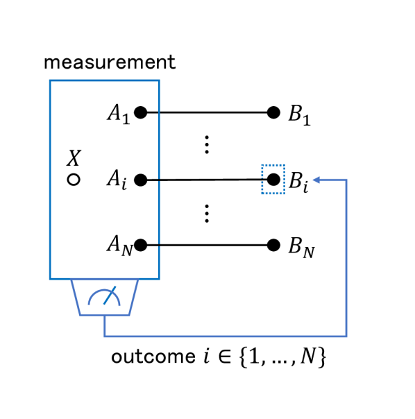
(a) port-based teleportation

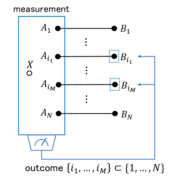
(b) port-based telecloning

Figure 1: (a) The setting of port-based teleportation (PBT). Alice and Bob share entangled states in the ports $A_{1},\ldots,A_{N}$ and $B_{1},\ldots,B_{N}$, with Alice also holding the input state in the system $X$. In the protocol, Alice first measures the systems $XA_{1}\cdots A_{N}$, and sends the outcome $i\in\{1,\ldots,N\}$ to Bob, who then selects port $B_{i}$. This completes the protocol. (b) The setting of port-based telecloning (PBTC). PBTC is best thought of as having $N$ receivers, where the $i$-th receiver has port $B_{i}\ (i=1,\ldots,N)$, and the goal of the protocol is to have $M$ receivers get approximate copies of the state of system $X$. In the protocol, Alice performs a measurement with a multi-index outcome, i.e., a subset $\{i_{1},\ldots,i_{M}\}\subset\{1,\ldots,N\}$, and sends the outcome to all receivers. Each receiver keeps their port if their port number is contained in Alice’s outcome. This completes the protocol, and a approximate copy of the input state of $X$ is transferred to $M$ receivers.

For a finite-dimensional Hilbert space $\mathcal{H}$, $\mathcal{L}(\mathcal{H})$ denotes the space of linear operators on $\mathcal{H}$. In PBT, Alice (the sender) and Bob (the receiver) share an entangled state $\Phi_{A^{N}B^{N}}\in\mathcal{L}\big{(}\mathcal{H}^{\otimes N}\otimes\mathcal{H}^{\otimes N}\big{)}$ on $2N$ qudits, and Alice has the input pure state $\sigma_{X}\in\mathcal{L}(\mathcal{H}_{X})$. Here, system $A^{N}\equiv A_{1}\cdots A_{N}\ (B^{N}\equiv B_{1}\cdots B_{N})$ is on Alice’s (Bob’s) side. Each system $A$ is associated with a finite-dimensional Hilbert space $\mathcal{H}_{A}\cong\mathbbm{C}^{d}$. Shared entangled state $\Phi_{A^{N}B^{N}}$ is called a resource state, and each of systems $A_{1},\ldots,A_{N},B_{1},\ldots,B_{N}$ is referred to as a port.

The protocol of PBT is as follows:

1. Alice jointly measures the input system $X$ and all her ports $A^{N}$ with a POVM $\{E^{i}_{XA^{N}}\}_{i=1}^{N}$.

2. Alice tells the outcome $i\in\{1,\ldots,N\}$ to Bob via classical communication.

3. Bob selects the port $B_{i}$ and discards all other ports $B^{N}\setminus B_{i}$.

This completes the protocol and the state is transferred to the remaining port $B_{i}$. The PBT channel $\mathcal{E}_{N}:\mathcal{L}(\mathcal{H}_{X})\rightarrow\mathcal{L}(\mathcal{H}_{B})$ is then expressed as follows:

$$\mathcal{E}_{N}(\sigma_{X})=\sum_{i=1}^{N}\operatorname{Tr}_{XA^{N}B_{i}^{c}}\left[E^{i}_{XA^{N}}\left(\sigma_{X}\otimes\Phi_{A^{N}B^{N}}\right)\right],$$ (1)

where $B_{i}^{c}\equiv B^{N}\setminus B_{i}=B_{1}\cdots B_{i-1}B_{i+1}\cdots B_{N}$ and the remaining system $B_{i}$ is relabeled as output system $B$. The left side of Figure 1 represents PBT [3].

The performance of PBT is evaluated by entanglement fidelity. The entanglement fidelity $F$ of a quantum channel $\mathcal{N}:\mathcal{L}(\mathcal{H})\rightarrow\mathcal{L}(\mathcal{\mathcal{H}})$ is defined as follows.

$$F(\mathcal{N})\coloneq\bra{\Phi^{+}}\left(\mathcal{N}\otimes\mathrm{id}\right)\left(\Phi^{+}\right)\ket{\Phi^{+}},$$ (2)

where $\Phi^{+}=\ket{\Phi^{+}}\bra{\Phi^{+}}$ is the maximally entangled state defined by $\ket{\Phi^{+}}=\frac{1}{\sqrt{d}}\sum_{i=1}^{d}\ket{i}\ket{i}$ for orthonormal basis $\{\ket{i}\}_{i=1}^{d}$, and $\mathrm{id}$ is the identity channel. Entanglement fidelity is related to average output fidelity $f$, which is defined as follows:

$$f(\mathcal{N})\coloneq\int\mathrm{d}\phi\bra{\phi}\mathcal{N}(\phi)\ket{\phi},$$ (3)

where the integral is performed with respect to the uniform distribution $\mathrm{d}\phi$ over all input pure state. These two quantities are connected by the following relationship [21]:

$$f(\mathcal{N})=\frac{F(\mathcal{N})d+1}{d+1}.$$ (4)

An important class of POVM in PBT is the pretty good measurement (PGM) [22, 23]. The PGM $\{E^{i}\}_{i}$ for the state ensemble $\{(p_{i},\sigma^{i})\}_{i\in\mathcal{I}}$ is given by

$$E^{i}=\bar{\sigma}^{-\frac{1}{2}}p_{i}\sigma^{i}\bar{\sigma}^{-\frac{1}{2}},$$ (5)

where $\bar{\sigma}=\sum_{i\in\mathcal{I}}p_{i}\sigma^{i}$ and $\bar{\sigma}^{-1}$ is defined on the support of $\bar{\sigma}$, which can always be assumed to be invertible, without loss of generality. In [4, 11], it is shown that the POVM that maximizes the fidelity of PBT is the PGM constructed from the ensemble $\{(1/N,\ \rho^{i}_{XA^{N}})\}_{i=1}^{N}$, where

$$\rho^{i}_{XA^{N}}\coloneq\Phi^{+}_{XA_{i}}\otimes\frac{1}{d^{N-1}}\mathbbm{1}_{A_{i}^{c}}\;.$$ (6)

A PBT protocol that uses $N$ pairs of maximally entangled states as ports, and the PGM for $\{(1/N,\ \rho^{i}_{XA^{N}})\}_{i=1}^{N}$ as measurement, is called standard PBT. The entanglement fidelity of standard PBT channel $\mathcal{E}^{\mathrm{std}}_{N}$ is computed as follows [10]:

$$F(\mathcal{E}^{\mathrm{std}}_{N})=1-\frac{d^{2}-1}{4N}+O\left(N^{-\frac{3}{2}+\delta}\right),$$ (7)

where $\delta>0$. In addition, we can consider using any resource state, not limited to maximally entangled states. Even in this case, it is known that the PGM that is the same as the POVM used in standard PBT is optimal (i.e., maximizing entanglement fidelity) [11]. If we denote a PBT channel using the PGM and optimal resource states as $\mathcal{E}^{\mathrm{opt}}_{N}$, its performance can be expressed as follows [10]:

$$F(\mathcal{E}^{\mathrm{opt}}_{N})=1-\Theta(N^{-2}).$$ (8)

II.2 Telecloning

Telecloning [14, 15] is a generalization of ST to the case of many receivers. The objective of telecloning is to distribute one input state to many distant receivers. However, the no-cloning theorem [17] prohibits making multiple perfect copies of a single unknown state. The best a sender can do is to transfer an optimal clone that is the closest to the original state allowed by quantum mechanics. In the following, we will focus on symmetric cloning, i.e., the situation where there is no difference between the copies that each recipient receives.

The $K\rightarrow M$ optimal cloning map $\mathcal{C}:\mathcal{L}(\mathcal{H}^{\otimes K})\rightarrow\mathcal{L}(\mathcal{H}^{\otimes M})$ given by Werner [20] is obtained by projecting $K$ input copies and $M-K$ completely mixed state onto a symmetric subspace:

$$\mathcal{C}\left(\ket{\phi}\bra{\phi}^{\otimes K}\right)=\frac{d[K]}{d[M]}\Pi_{M}\left(\ket{\phi}\bra{\phi}^{\otimes K}\otimes\mathbbm{1}^{\otimes M-K}\right)\Pi_{M},$$ (9)

where $d[K]=\binom{d+K-1}{K}$ and $\Pi_{M}$ is the projection onto the totally symmetric subspace of $\mathcal{H}^{\otimes M}$. The state in (9) optimizes also the fidelity of each clone [24], which is written as follows:

$$\mathcal{R}\circ\mathcal{C}\left(\ket{\phi}\bra{\phi}^{\otimes K}\right)=\gamma_{K,M}\ket{\phi}\bra{\phi}+(1-\gamma_{K,M})\frac{1}{d}\mathbbm{1},$$ (10)

where $\gamma_{K,M}=\frac{K}{M}\frac{M+d}{K+d}$ and $\mathcal{R}$ represents the trace over all subsystems except the first one (due to exchange symmetry all clones are equal). Furthermore, since $\mathcal{C}$ is universal (i.e., the fidelity does not depend on the input pure states), the fidelity for $K=1$ is given as follows:

$$f(\mathcal{R}\circ\mathcal{C}) =\gamma_{1,M}+(1-\gamma_{1,M})\frac{1}{d}$$

$$=\frac{d+2M-1}{M(d+1)}.$$ (11)

There is a straightforward protocol to transfer optimal clones to many receivers. That is, Alice applies the optimal cloning map locally and transfers its output to each receiver by ST. If the number of clones is $M$, this protocol requires $M\log_{2}d$ ebits. Unlike this “clone-and-teleport” protocol, the protocol introduced in [14, 15] performs cloning and teleportation simultaneously. An advantage of this protocol is that it only requires $\log_{2}d$ ebits entanglement between the sender and the receivers. This is achieved by using the $2M$ qudits entangled state, called a telecloning state, which is shared between Alice and the $2M-1$ receivers (each participant has one qudit). The protocol is as follows:

1. Alice performs a complete $d$-dimensional Bell measurement on the input state and her entangled state.

2. Alice tells the outcome to all receivers via classical communication.

3. Each receiver applies an appropriate unitary transformation based on Alice’s measurement outcome.

This completes the protocol, and $M$ receivers obtain the optimal clone of the input state. This is possible because the universal cloning is covariant under the action of the unitary group.

III Port-based telecloning

III.1 The protocol

In this section, we introduce PBTC, which performs telecloning using PBT. The goal of PBTC is to distribute $M$ copies of the state of the input system across $N$ ports in one go. In particular, we consider a symmetric cloning scenario, i.e., all copies should look the same locally.

In PBTC, we use a POVM whose outcomes specify a subset of all ports available: the ports contained in such a subset will receive a copy of the input state, whereas the remaining ports will be discarded. The set of measurement outcomes is defined as follows.

Definition 1.

For fixed $N,M\ (N\geq M)$, defining the set

$$\mathcal{I}_{N}^{M}\coloneq\{\{i_{1},\ldots,i_{M}\}\ |\ i_{k}\in\{1,\ldots,N\}\ \mathrm{for}\ k\in\{1,\ldots,M\},$$

$$\mathrm{and}\ i_{1}<\cdots<i_{M}\}.$$ (12)

Here, $|\mathcal{I}_{N}^{M}|=\binom{N}{M}$. For $I=\{i_{1},\ldots,i_{M}\}\in\mathcal{I}_{N}^{M}$, we write the composite system $A_{I}\equiv A_{i_{1}}\cdots A_{i_{M}}$ and $A_{I}^{c}\equiv A^{N}\setminus A_{I}$.

The right side of Figure 1 represents PBTC. In PBTC, Alice and $N$ receivers share an resource state $\Phi_{A^{N}B^{N}}$. We consider Alice has ports $A_{1},\ldots,A_{N}$, and the $i$-th receiver has the port $B_{i}\ (i=1,\ldots,N)$. Additionally, Alice holds the input state $\sigma_{X}$. The protocol of PBTC is as follows:

1. Alice measures the input system $X$ and all her ports $A^{N}$ with a POVM $\{E^{I}_{XA^{N}}\}_{I\in\mathcal{I}_{N}^{M}}$.

2. Alice tells the outcome $I\in\mathcal{I}_{N}^{M}$ to all receivers via classical communication.

3. The $i$-th receiver discards their port $B_{i}$ if $i\notin I$ and does nothing if $i\in I$ $(i=1,\ldots,N)$.

This completes the protocol, and the clones are transferred to the $M$ receivers. The PBTC channel $\mathcal{D}_{N,M}:\mathcal{L}(\mathcal{H}_{X})\rightarrow\mathcal{L}(\mathcal{H}^{\otimes M})$ is expressed as follows:

$$\mathcal{D}_{N,M}(\sigma_{X})=\sum_{I\in\mathcal{I}_{N}^{M}}\operatorname{Tr}_{XA^{N}B_{I}^{c}}\left[E^{I}_{XA^{N}}\left(\sigma_{X}\otimes\Phi_{A^{N}B^{N}}\right)\right],$$ (13)

and the remaining system $B_{i_{k}}$ $(k=1,\ldots,M)$ is relabeled as output system $B_{k}$.

Clone-and-teleport protocol

In Sec. II.2, we described a trivial “clone-and-teleport” protocol for telecloning, and we can consider a similar protocol for PBTC. The protocol is that Alice creates an optimal $M$-clone locally and transfers it by multi port-based teleportation (MPBT) [25]. For simplicity, we only consider $1\to M$ cloning.

MPBT is the protocol that transfers $M$ qudits states to $M$ ports in one go. The POVM for MPBT using $N$ pairs of maximally entangled states is given by the PGM for $\{(|\mathcal{J}_{N}^{M}|^{-1},\rho^{J}_{X^{M}A^{N}})\}_{J\in\mathcal{J}_{N}^{M}}$, where

$$\mathcal{J}_{N}^{M}\coloneq\{(j_{1},\ldots,j_{M})\ |\ j_{k}\in\{1,\ldots,N\}\ \mathrm{for}\ k\in\{1,\ldots,M\},$$

$$\mathrm{and}\ j_{k}\neq j_{l}\ \mathrm{for}\ k\neq l\}$$ (14)

is the ordered version of $\mathcal{I}_{N}^{M}$, and for $J=(j_{1},\ldots,j_{M})\in\mathcal{J}_{N}^{M}$,

$$\rho^{J}_{X^{M}A^{N}}\coloneq\bigotimes_{k=1}^{M}\Phi^{+}_{X_{k}A_{j_{k}}}\otimes\frac{1}{d^{N-M}}\mathbbm{1}_{A_{J}^{c}}.$$ (15)

We refer to the protocol that performs optimal cloning and MPBT successively as clone-and-MPBT protocol. Clone-and-MPBT protocol can be considered in the framework of PBTC. Clone-and-MPBT protocol is equivalent to PBTC using POVM

$$\big{\{}(\mathcal{C}^{\dagger}_{X^{M}\rightarrow X}\otimes\mathrm{id}_{A^{N}})(E^{J}_{X^{M}A^{N}})\big{\}}_{J\in\mathcal{J}_{N}^{M}},$$ (16)

where $\mathcal{C}^{\dagger}_{X^{M}\rightarrow X}:\mathcal{L}(\mathcal{H}^{\otimes M}_{X^{M}})\rightarrow\mathcal{L}(\mathcal{H}_{X})$ is the adjoint of optimal cloning map given by (9), and $\{E^{J}_{X^{M}A^{N}}\}_{J\in\mathcal{J}_{N}^{M}}$ is the PGM for $\{(|\mathcal{J}_{N}^{M}|^{-1},\rho^{J}_{X^{M}A^{N}})\}_{J\in\mathcal{J}_{N}^{M}}$. The set of measurement outcomes in (16) is not $\mathcal{I}_{N}^{M}$, but this poses no issue because it can be made equivalent to $\mathcal{I}_{N}^{M}$ by summing the POVM elements for outcomes that are identical when reordered.

Note that the sum of $E^{i}$ defined by (5) is the projection onto the support of $\bar{\sigma}$, which generally does not coincide with the identity operator. One way to make them POVM in the full Hilbert space is adding

$$\Delta=\frac{1}{|\mathcal{I}|}\left(\mathbbm{1}-\sum_{i\in\mathcal{I}}E^{i}\right)$$ (17)

to each $E^{i}$. This does not change the argument in the original PBT since $\operatorname{Tr}[\Delta\sigma^{i}]=0$. However, on the other hand, because our figure of merit for (16) differs from the original PGM, it is essential to make $\{E^{i}\}$ a proper POVM in the full Hilbert space. Thus, we take into account $\Delta$ in clone-and-MPBT protocol.

Clone-and-MPBT protocol can transfer optimal clones in the limit of the number of ports $N\rightarrow\infty$. However, optimality for finite $N$ is not guaranteed. In fact, the POVM we introduce in the next subsection achieves higher fidelity than the clone-and-MPBT protocol when $N$ is small.

III.2 Generalization of POVM

As we have noted, in this work, we consider only symmetric cloning. We first introduce an ensemble for a PGM by partially symmetrizing the state $\rho^{i}_{XA^{N}}$ that constitutes the optimal POVM of PBT.

Definition 2.

For $I=\{i_{1},\ldots,i_{M}\}\in\mathcal{I}_{N}^{M}$, let

$$\eta^{I}_{XA^{N}}\coloneq\frac{d^{M}}{d[M]}\Pi_{A_{I}}\rho^{i_{1}}_{XA^{N}}\Pi_{A_{I}},$$ (18)

where $\rho^{i_{1}}_{XA^{N}}$ is the state given by (6), and $\Pi_{A_{I}}$ is the projection onto the symmetric subspace of $\mathcal{H}^{\otimes M}_{A_{I}}$.

In equation (18), although we formally use $i_{1}$ as the index of $\rho^{i_{1}}_{XA^{N}}$, note that $\eta^{I}_{XA^{N}}$ remains in the same state regardless of whether $i_{1}$ is replaced by any of the element of $I=\{i_{1},\ldots,i_{M}\}$.

We refer to PBTC that uses $N$ pairs of maximally entangled states and the PGM for $\{(|\mathcal{I}_{N}^{M}|^{-1},\eta^{I}_{XA^{N}})\}_{I\in\mathcal{I}_{N}^{M}}$ as standard PBTC. Since standard PBTC is symmetric cloning, we evaluate its performance by an average fidelity of single clone for all input pure states.

The asymptotic fidelity of standard PBTC is given by the following theorem.

Theorem 3.

Let us consider standard PBTC channel $\mathcal{D}^{\mathrm{std}}_{N,M}$ and the channel $\mathcal{R}$ that represents the trace over all subsystems except the first one. In the limit of the number of ports $N\rightarrow\infty$, the following equality holds:

$$\lim_{N\to\infty}f(\mathcal{R}\circ\mathcal{D}^{\mathrm{std}}_{N,M})=\frac{d+2M-1}{M(d+1)},$$ (19)

where $d$ is the dimension of the local Hilbert space and $M$ is the number of clones to be transferred.

The proof is given in Subsection III.3. The value of (19) coincides with the fidelity of $1\rightarrow M$ optimal cloning given by (11). Therefore, standard PBTC can transfer optimal clones asymptotically.

Finally, we numerically compare the performance of standard PBTC with clone-and-MPBT protocol described in the previous subsection. Figure 2 shows the fidelity of each protocol obtained by numerical calculation. Fidelity is calculated for a single clone. Namely, it represents $f(\mathcal{R}\circ\mathcal{D}^{\mathrm{std}}_{N,M})$ and $f(\mathcal{R}\circ\mathcal{T}_{N,M})$, where $\mathcal{D}^{\mathrm{std}}_{N,M}$ is the standard PBTC channel and $\mathcal{T}_{N,M}$ is the quantum channel corresponding to clone-and-MPBT protocol. The figure shows that standard PBTC achieves higher fidelity compared to clone-and-MPBT protocol when $\nobreak{d=2},\ \nobreak{M=2},\ \nobreak{2\leq N\leq 6}$. Due to the increasing complexity of the calculation we were not able to go to higher values of $M$ and $N$, but we conjecture that a finite gap exists for all finite values.

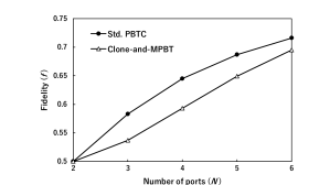
Figure 2: The fidelity of the PBTC protocol proposed here (circles) and the trivial clone-and-MPBT protocol (triangles). The plotted values have been obtained by numerical calculation for $d=2,\ M=2$. Fidelity is the average over the input pure state and is calculated for a single clone.

III.3 Proof of Theorem 3

In this subsection, we prove Theorem 3. Within this section, we use the same notation for operators on the systems $A^{N}B$ as we did for operators on the systems $XA^{N}$ in the previous sections, via the isomorphism $X\cong B$. For example, for $\rho^{i}_{XA^{N}}=\Phi^{+}_{XA_{i}}\otimes\frac{1}{d^{N-1}}\mathbbm{1}_{A_{i}^{c}}$ defined by (6), we have $\rho^{i}_{A^{N}B}=\Phi^{+}_{A_{i}B}\otimes\frac{1}{d^{N-1}}\mathbbm{1}_{A_{i}^{c}}$.

We start from showing the properties related to the symmetric group.

Definition 4.

Let $S_{N}$ be the symmetric group on $\{1,\ldots,N\}$, and for $I\in\mathcal{I}_{N}^{M}$, $S_{I}$ be the subgroup of $S_{N}$ consisting of all permutations of $I=\{i_{1},\ldots,i_{M}\}$. For $\sigma\in S_{N}$, the action of the unitary representation $V_{\sigma}\in\mathcal{L}(\mathcal{H}^{\otimes N})$ is defined follows:

$$V_{\sigma}\ket{k_{1}\cdots k_{N}}\coloneq\ket{k_{\sigma^{-1}(1)}\cdots k_{\sigma^{-1}(N)}}.$$ (20)

In addition, for $I\in\mathcal{I}_{N}^{M}$, let $\Pi_{A_{I}}$ be the projection onto the symmetric subspace of $\mathcal{H}^{\otimes M}_{A_{I}}$ as follows:

$$\Pi_{A_{I}}\coloneq\frac{1}{M!}\sum_{\sigma\in S_{I}}V_{\sigma}.$$ (21)

Note that although $\Pi_{A_{I}}$ defined by (21) is an operator on $\mathcal{H}^{\otimes N}_{A^{N}}$, it acts non-trivially only on $\mathcal{H}^{\otimes M}_{A_{I}}$.

Lemma 5.

For any $\sigma\in S_{N}$ and $I\in\mathcal{I}_{N}^{M}$, $\sigma S_{I}\sigma^{-1}=~S_{\sigma(I)}$.

Proof.

First, if $\tau\in\sigma S_{I}\sigma^{-1}$, there exists a $\pi\in S_{I}$ such that $\tau=\sigma\pi\sigma^{-1}$. Since $\sigma\pi\sigma^{-1}$ is a bijection on $\sigma(I)$, $\tau$ is a permutation of $\sigma(I)$. Thus, $\sigma S_{I}\sigma^{-1}\subset S_{\sigma(I)}$. Next, suppose $\tau\in S_{\sigma(I)}$. In this case, $\sigma^{-1}\tau\sigma$ is a bijection on $I$. Therefore, there exists a $\pi\in S_{I}$ such that $\sigma^{-1}\tau\sigma=\pi$. Since $\tau=\sigma\pi\sigma^{-1}$, and $\sigma\pi\sigma^{-1}\in\sigma S_{I}\sigma^{-1}$, we have $\tau\in\sigma S_{I}\sigma^{-1}$. Therefore, $S_{\sigma(I)}\subset\sigma S_{I}\sigma^{-1}$. ∎

Corollary 6.

For any $\sigma\in S_{N}$ and $I\in\mathcal{I}_{N}^{M}$, $V_{\sigma}\Pi_{A_{I}}V_{\sigma}^{\dagger}=\Pi_{A_{\sigma(I)}}$.

Proof.

From Lemma 5, we have

$$\sum_{\tau\in S_{I}}V_{\sigma\tau\sigma^{-1}}=\sum_{\pi\in S_{\sigma(I)}}V_{\pi}.$$ (22)

Since $V_{\sigma\pi}=V_{\sigma}V_{\pi}$ and $V_{\sigma^{-1}}=V_{\sigma}^{\dagger}$ for any $\sigma,\pi\in S_{N}$, the lemma holds. ∎

Proposition 7.

Let $\left\{E^{I}_{A^{N}B}\right\}_{I\in\mathcal{I}_{N}^{M}}$ be the PGM for $\{(|\mathcal{I}_{N}^{M}|^{-1},\eta^{I}_{A^{N}B})\}_{I\in\mathcal{I}_{N}^{M}}$. For any $I=\{i_{1},\ldots,i_{M}\}\in\mathcal{I}_{N}^{M}$, it holds that $\Pi_{A_{I}}E^{I}_{A^{N}B}\Pi_{A_{I}}=E^{I}_{A^{N}B}$.

Proof.

Let us denote

$$\bar{\eta}_{A^{N}B}=\binom{N}{M}^{-1}\sum_{I\in\mathcal{I}_{N}^{M}}\eta^{I}_{A^{N}B}.$$ (23)

For any $\sigma\in S_{N}$, we have

$$V_{\sigma}\bar{\eta}_{A^{N}B}$$

$$= {\binom{N}{M}}^{-1}\frac{d^{M}}{d[M]}\sum_{I\in\mathcal{I}_{N}^{M}}V_{\sigma}\Pi_{A_{I}}\rho^{i_{1}}_{A^{N}B}\Pi_{A_{I}}$$

$$= {\binom{N}{M}}^{-1}\frac{d^{M}}{d[M]}\sum_{I\in\mathcal{I}_{N}^{M}}V_{\sigma}\Pi_{A_{I}}V_{\sigma}^{\dagger}V_{\sigma}\rho^{i_{1}}_{A^{N}B}V_{\sigma}^{\dagger}V_{\sigma}\Pi_{A_{I}}V_{\sigma}^{\dagger}V_{\sigma}$$

$$= {\binom{N}{M}}^{-1}\frac{d^{M}}{d[M]}\sum_{I\in\mathcal{I}_{N}^{M}}\Pi_{A_{\sigma(I)}}\rho^{\sigma(i_{1})}_{A^{N}B}\Pi_{A_{\sigma(I)}}V_{\sigma}$$

$$= \bar{\eta}_{A^{N}B}V_{\sigma}$$ (24)

The second equality uses $V_{\sigma}^{-1}=V_{\sigma}^{\dagger}$, and the third equality uses $V_{\sigma}\rho^{i_{1}}_{A^{N}B}V_{\sigma}^{\dagger}=\rho^{\sigma(i_{1})}_{A^{N}B}$ and Corollary 6. Note that from the symmetry ${\binom{N}{M}}^{-1}\frac{d^{M}}{d[M]}\sum_{I\in\mathcal{I}_{N}^{M}}\Pi_{A_{\sigma(I)}}\rho^{\sigma(i_{1})}_{A^{N}B}\Pi_{A_{\sigma(I)}}={\bar{\eta}}_{A^{N}B}$ holds. By summing both sides with respect to $\sigma\in S_{I}$ and divide by $M!$, we obtain

$$\Pi_{A_{I}}\bar{\eta}_{A^{N}B}=\bar{\eta}_{A^{N}B}\Pi_{A_{I}}.$$ (25)

Since $\bar{\eta}^{-1}_{A^{N}B}$ is defined on the support of $\bar{\eta}_{A^{N}B}$, $\big{[}\Pi_{A_{I}},\bar{\eta}^{-\frac{1}{2}}_{A^{N}B}\big{]}=0$ also holds. Therefore,

$$\Pi_{A_{I}}E^{I}_{A^{N}B}\Pi_{A_{I}}$$

$$= \Pi_{A_{I}}\bar{\eta}_{A^{N}B}^{-\frac{1}{2}}\left(\frac{d^{M}}{d[M]}\Pi_{A_{I}}\rho^{i_{1}}_{A^{N}B}\Pi_{A_{I}}\right)\bar{\eta}_{A^{N}B}^{-\frac{1}{2}}\Pi_{A_{I}}$$

$$= \bar{\eta}_{A^{N}B}^{-\frac{1}{2}}\left(\frac{d^{M}}{d[M]}\Pi_{A_{I}}\rho^{i_{1}}_{A^{N}B}\Pi_{A_{I}}\right)\bar{\eta}_{A^{N}B}^{-\frac{1}{2}}$$

$$= E^{I}_{A^{N}B}.$$ (26)

∎

We then calculate the entanglement fidelity. The following lemma connects the entanglement fidelity of PBT with the state discrimination problem.

Lemma 8 ([4, 5]).

Let us fix the resource state to be $N$ pairs of maximally entangled states. The entanglement fidelity of the PBT channel $\mathcal{E}_{N}$ using the POVM $\{E^{i}_{XA^{N}}\}_{i=1}^{N}$ is given by:

$$F(\mathcal{E}_{N})=\frac{1}{d^{2}}\sum_{i=1}^{N}\operatorname{Tr}\left[E^{i}_{A^{N}B}\rho^{i}_{A^{N}B}\right].$$ (27)

By applying this lemma for standard PBTC, we obtain the following as a corollary.

Corollary 9.

Let us consider standard PBTC channel $\mathcal{D}^{\mathrm{std}}_{N,M}$ and quantum channel $\mathcal{R}$ that traces over all subsystems except the first one. The entanglement fidelity of the quantum channel $\mathcal{R}\circ\mathcal{D}^{\mathrm{std}}_{N,M}$ is given by:

$$F(\mathcal{R}\circ\mathcal{D}^{\mathrm{std}}_{N,M})=\frac{1}{d^{2}}\sum_{I\in\mathcal{I}_{N}^{M}}\operatorname{Tr}\left[E^{I}_{A^{N}B}\rho^{i_{1}}_{A^{N}B}\right],$$ (28)

where $i_{1}$ is the smallest number of $I$, and $\{E^{I}_{XA^{N}}\}_{I\in\mathcal{I}_{N}^{M}}$ is the PGM for $\{(|\mathcal{I}_{N}^{M}|^{-1},\eta^{I}_{A^{N}B})\}_{I\in\mathcal{I}_{N}^{M}}$.

The following lemma provides a lower bound of the success probability for the state discrimination problem of PGM. It is proportional to the entanglement fidelity, as expressed by Lemma 8.

Lemma 10 ([5]).

Let $\{E^{i}\}_{i=1}^{N}$ be the PGM for any state ensemble $\{(1/N,\sigma^{i})\}_{i=1}^{N}$. Then, the success probability for the state discrimination problem

$$p_{\mathrm{succ}}=\frac{1}{N}\sum_{i=1}^{N}\operatorname{Tr}\left[E^{i}\sigma^{i}\right]$$ (29)

satisfies the following inequality:

$$p_{\mathrm{succ}}\geq\frac{1}{N\bar{r}\operatorname{Tr}\bar{\sigma}^{2}},$$ (30)

where

$$\bar{r}=\frac{1}{N}\sum_{i=1}^{N}\operatorname{rank}{\sigma^{i}}\ ,\ \bar{\sigma}=\frac{1}{N}\sum_{i=1}^{N}{\sigma^{i}}.$$ (31)

To utilize Lemma 10, we calculate the values of (31) for the state ensemble $\{(|\mathcal{I}_{N}^{M}|^{-1},\eta^{I}_{XA^{N}})\}_{I\in\mathcal{I}_{N}^{M}}$. The average rank is given by the following proposition.

Proposition 11.

$\binom{N}{M}^{-1}\sum_{I\in\mathcal{I}_{N}^{M}}\operatorname{rank}{\eta^{I}_{A^{N}B}}=d[M-1]d^{N-M}.$

Proof.

For any $I=\{i_{1},\ldots,i_{M}\}\in\mathcal{I}_{N}^{M}$, we have

$$\eta^{I}_{A^{N}B}=\frac{d^{M-N+1}}{d[M]}\Pi_{A_{I}}(\Phi^{+}_{A_{i_{1}}B}\otimes\mathbbm{1}_{A_{I}\setminus A_{i_{1}}})\Pi_{A_{I}}\otimes\mathbbm{1}_{A_{I}^{c}}.$$ (32)

The set $W$ of eigenvectors corresponding to the non-zero eigenvalues of $\Pi_{A_{I}}(\Phi^{+}_{A_{i_{1}}B}\otimes\mathbbm{1}_{A_{I}\setminus A_{i_{1}}})\Pi_{A_{I}}$ is

$$W=\left\{\Pi_{A_{I}}\ket{\Phi^{+}}_{A_{i_{1}}B}\ket{k_{1}\cdots k_{M-1}}_{A_{I}\setminus A_{i_{1}}}\right\}_{k_{1},\ldots,k_{M-1}=1}^{d},$$ (33)

where $\{\ket{k}\}_{k=1}^{d}$ is the orthonormal basis of $\mathcal{H}$. Since $\operatorname{rank}\mathbbm{1}_{A_{I}^{c}}=d^{N-M}$, it is sufficient to show $|W|=d[M-1]$. Here,

$$\Pi_{A_{I}}\ket{\Phi^{+}}_{A_{i_{1}}B}\ket{k_{1}\cdots k_{M-1}}_{A_{I}\setminus A_{i_{1}}}$$

$$= \frac{1}{\sqrt{d}}\sum_{i=1}^{d}\Pi_{A_{I}}\ket{i\ k_{1}\cdots k_{M-1}}_{A_{I}}\ket{i}_{B}.$$ (34)

Thus,

$$\Pi_{A_{I}}\ket{\Phi^{+}}_{A_{i_{1}}B}\ket{k_{1}\cdots k_{M-1}}_{A_{I}\setminus A_{i_{1}}}$$

$$= \Pi_{A_{I}}\ket{\Phi^{+}}_{A_{i_{1}}B}\ket{l_{1}\cdots l_{M-1}}_{A_{I}\setminus A_{i_{1}}}$$ (35)

holds for $k_{1},\ldots,k_{M-1},l_{1},\ldots,l_{M-1}\in\{1,\ldots d\}$ if and only if

$$\Pi_{A_{I}}\ket{i\ k_{1}\cdots k_{M-1}}_{A_{I}}=\Pi_{A_{I}}\ket{i\ l_{1}\cdots l_{M-1}}_{A_{I}}$$ (36)

holds for each $i\in\{1,\ldots,d\}$. Eq. (36) holds if and only if $k_{1},\ldots,k_{M-1}$ and $l_{1},\ldots,l_{M-1}$ match after permutation. Thus, $|W|$ equals the number of combinations with repetition of selecting $M-1$ elements from $\{1,\ldots,d\}$. Hence, $|W|=d[M-1]$. ∎

Next, we estimate $\operatorname{Tr}{\bar{\eta}^{2}_{A^{N}B}}$.

Lemma 12.

Let $I,J,K,L\in\mathcal{I}_{N}^{M}$. If $|I\cap J|=|K\cap L|$, then $\operatorname{Tr}\left[\eta^{I}_{A^{N}B}\eta^{J}_{A^{N}B}\right]=\operatorname{Tr}\left[\eta^{K}_{A^{N}B}\eta^{L}_{A^{N}B}\right]$.

Proof.

For any $\sigma\in S_{N}$ and $I=\{i_{1},\ldots,i_{M}\}\in\mathcal{I}_{N}^{M}$, we have

$$\eta^{I}_{A^{N}B} =\frac{d^{M}}{d[M]}\Pi_{A_{I}}\rho^{i_{1}}_{A^{N}B}\Pi_{A_{I}}$$

$$=\frac{d^{M}}{d[M]}V_{\sigma}^{\dagger}V_{\sigma}\Pi_{A_{I}}V_{\sigma}^{\dagger}V_{\sigma}\rho^{i_{1}}_{A^{N}B}V_{\sigma}^{\dagger}V_{\sigma}\Pi_{A_{I}}V_{\sigma}^{\dagger}V_{\sigma}$$

$$=\frac{d^{M}}{d[M]}V_{\sigma}^{\dagger}\Pi_{A_{\sigma(I)}}\rho^{\sigma(i_{1})}_{A^{N}B}\Pi_{A_{\sigma(I)}}V_{\sigma}$$

$$=V_{\sigma}^{\dagger}\eta^{\sigma(I)}_{A^{N}B}V_{\sigma}.$$ (37)

The second equality uses $V_{\sigma}^{-1}=V_{\sigma}^{\dagger}$, and the third equality uses $V_{\sigma}\rho^{i_{1}}_{A^{N}B}V_{\sigma}^{\dagger}=\rho^{\sigma(i_{1})}_{A^{N}B}$ and Corollary 6. Therefore, for any $\sigma\in S_{N}$ and $I,J\in\mathcal{I}_{N}^{M}$, we obtain

$$\operatorname{Tr}\left[\eta^{I}_{A^{N}B}\eta^{J}_{A^{N}B}\right] =\operatorname{Tr}\left[(V_{\sigma}^{\dagger}\eta^{\sigma(I)}_{A^{N}B}V_{\sigma})(V_{\sigma}^{\dagger}\eta^{\sigma(J)}_{A^{N}B}V_{\sigma})\right]$$

$$=\operatorname{Tr}\left[\eta^{\sigma(I)}_{A^{N}B}\eta^{\sigma(J)}_{A^{N}B}\right].$$ (38)

Note that $|I\cap J|=|\sigma(I)\cap\sigma(J)|$. Moreover, for any $K,L\in\mathcal{I}_{N}^{M}$ satisfying $|I\cap J|=|K\cap L|$, there exists $\sigma\in S_{N}$ such that $\sigma(I)=K,\sigma(J)=L$. Thus, the proposition is proved. ∎

Lemma 13.

For any $I,J\in\mathcal{I}_{N}^{M}$, it holds that $\operatorname{Tr}\left[\eta^{I}_{A^{N}B}\eta^{J}_{A^{N}B}\right]\leq\operatorname{Tr}\left[(\eta^{I}_{A^{N}B})^{2}\right]$.

Proof.

Applying the Cauchy-Schwarz inequality to the Hilbert-Schmidt inner product, we have

$$\left|\operatorname{Tr}[A^{\dagger}B]\right|\leq\sqrt{\operatorname{Tr}\left[A^{\dagger}A\right]}\sqrt{\operatorname{Tr}\left[B^{\dagger}B\right]}.$$ (39)

for any $A,B\in\mathcal{L}(\mathcal{H}^{\otimes N+1})$. By setting $A=\eta^{I}_{A^{N}B},\ B=V_{\sigma}\eta^{I}_{A^{N}B}V_{\sigma}^{\dagger}=\eta^{\sigma(I)}_{A^{N}B}$ for $\sigma\in S_{N}$, we obtain

$$\mathrm{LHS} =\left|\operatorname{Tr}\left[\eta^{I}_{A^{N}B}\eta^{\sigma(I)}_{A^{N}B}\right]\right|=\operatorname{Tr}\left[\eta^{I}_{A^{N}B}\eta^{\sigma(I)}_{A^{N}B}\right],$$ (40)

$$\mathrm{RHS} =\sqrt{\operatorname{Tr}\left[\eta^{I}_{A^{N}B}\eta^{I}_{A^{N}B}\right]}\sqrt{\operatorname{Tr}\left[(V_{\sigma}\eta^{I}_{A^{N}B}V_{\sigma}^{\dagger})(V_{\sigma}\eta^{I}_{A^{N}B}V_{\sigma}^{\dagger})\right]}$$

$$=\operatorname{Tr}\left[(\eta^{I}_{A^{N}B})^{2}\right].$$ (41)

Since $\sigma\in S_{N}$ is arbitrary, $J=\sigma(I)$ is arbitrary. ∎

Lemma 14.

For any $I\in\mathcal{I}_{N}^{M}$, the following inequality holds:

$$\operatorname{Tr}\left[(\eta^{I}_{A^{N}B})^{2}\right]\leq\frac{d^{M-N+2}}{d[M]}\frac{M!(M-1)!}{d+M-1}.$$ (42)

Proof.

From the arguments made in the proof of Proposition 11, $\eta^{I}_{A^{N}B}$ has $d[M-1]d^{N-M}$ non-zero eigenvalues, and its eigenvectors are given in the form

$$\Pi_{A_{I}}\ket{\Phi^{+}}_{A_{i_{1}}B}\ket{k_{1}\cdots k_{M-1}}_{A_{I}\setminus A_{i_{1}}}\ket{k_{M}\cdots k_{N-1}}_{A_{I}^{c}},$$ (43)

where $k_{1},\ldots,k_{N-1}\in\{1,\ldots,d\}$ and $\{\ket{k}\}_{k=1}^{d}$ is the orthonormal basis of $\mathcal{H}$. If there are $n$ different permutations to rearrange $k_{1},\ldots,k_{M-1}$ without distinguishing the same numbers, the eigenvalue corresponding to (43) is $n\frac{d^{M-N+1}}{d[M]}$. Since $n\leq(M-1)!$ is always holds, all $d[M-1]d^{N-M}$ non-zero eigenvalues are less than or equal to $(M-1)!\frac{d^{M-N+1}}{d[M]}$. Hence,

$$\operatorname{Tr}\left[(\eta^{I}_{A^{N}B})^{2}\right] \leq d[M-1]d^{N-M}\left((M-1)!\frac{d^{M-N+1}}{d[M]}\right)^{2}$$

$$=\frac{d^{M-N+2}}{d[M]}\frac{M!(M-1)!}{d+M-1}.$$ (44)

∎

Lemma 15.

Let $I,J\in\mathcal{I}_{N}^{M}$. If $I\cap J=\emptyset$, then $\operatorname{Tr}\big{[}\eta^{I}_{A^{N}B}\eta^{J}_{A^{N}B}\big{]}=1/d^{N+1}$.

Proof.

Suppose $I=\{i_{1},\ldots,i_{M}\},J=\{j_{1},\ldots,j_{M}\}$. When $I\cap J=\emptyset$, we have

$$\big{[}\Pi_{A_{I}},\Pi_{A_{J}}\big{]}=\big{[}\Pi_{A_{I}},\rho^{j_{1}}_{A^{N}B}\big{]}=\big{[}\Pi_{A_{J}},\rho^{i_{1}}_{A^{N}B}\big{]}=0.$$ (45)

Thus,

$$\operatorname{Tr}\left[\eta^{I}_{A^{N}B}\eta^{J}_{A^{N}B}\right]=\frac{d^{2M}}{(d[M])^{2}}\operatorname{Tr}\left[\Pi_{A_{I}}\rho^{i_{1}}_{A^{N}B}\Pi_{A_{J}}\rho^{j_{1}}_{A^{N}B}\right].$$ (46)

Therefore, with some calculations we obtain

$$\operatorname{Tr}\left[\eta^{I}_{A^{N}B}\eta^{J}_{A^{N}B}\right]$$

$$= \frac{1}{(d[M]M!)^{2}d^{N}}\sum_{\sigma\in S_{I}}\sum_{\tau\in S_{J}}\sum_{k_{i_{1}},\ldots,k_{i_{M}}=1}^{d}\sum_{l_{j_{1}},\ldots,l_{j_{M}}=1}^{d}$$

$$\times\delta_{l_{j_{1}},k_{\sigma^{-1}(i_{1})}}\delta_{k_{i_{1}},l_{\tau^{-1}(j_{1})}}\prod_{p=2}^{M}\delta_{k_{i_{p}},k_{\sigma^{-1}(i_{p})}}\delta_{l_{j_{p}},l_{\tau^{-1}(j_{p})}}.$$ (47)

For the detailed derivation of (47), see Appendix A. To calculate (47), we decompose $\sigma,\tau$ into cycles. Suppose $\sigma\in S_{I}$ can be decomposed into $\sigma=C_{1}^{\sigma}C_{2}^{\sigma}\cdots C_{l(\sigma)}^{\sigma}$ (including cycles with a single element), and let $c_{m}^{\sigma}$ represents the length of the cycle $C_{m}^{\sigma}$ (similarly for $\tau\in S_{J}$). Then, by definition,

$$\sum_{m=1}^{l(\sigma)}c_{m}^{\sigma}=\sum_{m=1}^{l(\tau)}c_{m}^{\tau}=M.$$ (48)

Furthermore, we denote the elements of the cycle as $C_{m}^{\sigma}=(i^{m}_{1}\ \cdots\ i^{m}_{c^{\sigma}_{i}}),\ C_{m}^{\tau}=(j^{m}_{1}\ \cdots\ j^{m}_{c^{\tau}_{j}})$. Without loss of generality, let $i_{1}=i_{1}^{1}$ and $j_{1}=j_{1}^{1}$. When $c^{\sigma}_{1}\neq 1$ and $c^{\tau}_{1}\neq 1$, it can be expressed as follows:

$$\delta_{l_{j_{1}},k_{\sigma^{-1}(i_{1})}}\delta_{k_{i_{1}},l_{\tau^{-1}(j_{1})}}\prod_{p=2}^{M}\delta_{k_{i_{p}},k_{\sigma^{-1}(i_{p})}}\delta_{l_{j_{p}},j_{\tau^{-1}(j_{p})}}$$

$$= \left(\delta_{l_{j^{1}_{1}},k_{\sigma^{-1}\left(i^{1}_{1}\right)}}\delta_{k_{i^{1}_{1}},l_{\tau^{-1}\left(j^{1}_{1}\right)}}\prod_{p=2}^{c^{\sigma}_{1}}\delta_{k_{i^{1}_{p}},k_{\sigma^{-1}\left(i^{1}_{p}\right)}}\prod_{q=2}^{c^{\tau}_{1}}\delta_{l_{j^{1}_{q}},l_{\tau^{-1}\left(j^{1}_{q}\right)}}\right)$$

$$\times\left(\prod_{m=2}^{l(\sigma)}\prod_{n=1}^{c^{\sigma}_{m}}\delta_{k_{i^{m}_{n}},k_{\sigma^{-1}\left(i^{m}_{n}\right)}}\right)\left(\prod_{s=2}^{l(\tau)}\prod_{t=1}^{c^{\tau}_{s}}\delta_{l_{j^{s}_{t}},l_{\tau^{-1}(j^{s}_{t})}}\right).$$ (49)

When $c^{\sigma}_{1}=1$ or $c^{\tau}_{1}=1$, $\prod_{p=2}^{c^{\sigma}_{1}}\delta_{k_{i^{1}_{p}},k_{\sigma^{-1}\left(i^{1}_{p}\right)}}$ or $\prod_{q=2}^{c^{\tau}_{1}}\delta_{l_{j^{1}_{q}},l_{\tau^{-1}\left(j^{1}_{q}\right)}}$ in (III.3) is disregarded, respectively. The right-hand side of (III.3) corresponds to cycles $C^{\sigma}_{1}$ and $C^{\tau}_{1}$ in the first parenthesis, $C^{\sigma}_{2},\ldots,C^{\sigma}_{l(\sigma)}$ in the second parenthesis, and $C^{\tau}_{2},\ldots,C^{\tau}_{l(\tau)}$ in the third parenthesis. When we sum (III.3) over $k_{i_{1}},\ldots,k_{i_{M}},l_{j_{1}},\ldots,l_{j_{M}}$, the first parenthesis eliminates $c^{\sigma}_{1}+c^{\tau}_{1}-1$ indices. The second parenthesis eliminates $c^{\sigma}_{m}-1$ indices for a fixed $m\in\{2,\ldots,l(\sigma)\}$, for a total of $\sum_{m=2}^{l(\sigma)}(c^{\sigma}_{m}-1)$ indices. Similarly, the third parenthesis eliminates $\sum_{s=2}^{l(\tau)}(c^{\tau}_{s}-1)$ indices. Consequently, the total number of eliminated indices for fixed $\sigma\in S_{I},\tau\in S_{J}$ is

$$(c^{\sigma}_{1}+c^{\tau}_{1}-1)+\sum_{m=2}^{l(\sigma)}(c^{\sigma}_{m}-1)+\sum_{s=2}^{l(\tau)}(c^{\tau}_{s}-1)$$

$$= \sum_{k=1}^{l(\sigma)}c_{k}^{\sigma}+\sum_{k=1}^{l(\tau)}c_{k}^{\tau}-1-(l(\sigma)-1)-(l(\tau)-1)$$

$$= 2M+1-l(\sigma)-l(\tau).$$ (50)

Since there were $2M$ indices of $k_{i_{1}},\ldots,k_{i_{M}},l_{j_{1}},\ldots,l_{j_{M}}$ at the beginning, the remaining indices are

$$2M-\left(2M+1-l(\sigma)-l(\tau)\right)=l(\sigma)+l(\tau)-1$$ (51)

Hence,

$$\sum_{k_{i_{1}},\ldots,k_{i_{M}}=1}^{d}\sum_{l_{j_{1}},\ldots,l_{j_{M}}=1}^{d}\delta_{l_{j_{1}},k_{\sigma^{-1}(i_{1})}}\delta_{k_{i_{1}},l_{\tau^{-1}(j_{1})}}$$

$$\times\prod_{p=2}^{M}\delta_{k_{i_{p}},k_{\sigma^{-1}(i_{p})}}\delta_{l_{j_{p}},l_{\tau^{-1}(j_{p})}}$$

$$= \ d^{l(\sigma)+l(\tau)-1}.$$ (52)

Here, the number of $\sigma\in S_{M}$ satisfying $l(\sigma)=k$ is given by the first kind Stirling number $\genfrac{[}{]}{0.0pt}{}{M}{k}$ (see Remark 16 for details). Therefore,

$$\sum_{\sigma\in S_{I}}\sum_{\tau\in S_{J}}d^{l(\sigma)+l(\tau)-1} =\left(\sum_{\sigma\in S_{I}}d^{l(\sigma)}\right)\left(\sum_{\tau\in S_{J}}d^{l(\tau)}\right)d^{-1}$$

$$=\left(\sum_{k=1}^{M}\genfrac{[}{]}{0.0pt}{}{M}{k}d^{k}\right)^{2}d^{-1}$$

$$=\frac{1}{d}\left(\frac{(M+d-1)!}{(d-1)!}\right)^{2}.$$ (53)

Thus,

$$\operatorname{Tr}\left[\eta^{I}_{A^{N}B}\eta^{J}_{A^{N}B}\right] =\frac{1}{(d[M]M!)^{2}d^{N}}\frac{1}{d}\left(\frac{(M+d-1)!}{(d-1)!}\right)^{2}$$

$$=\frac{1}{d^{N+1}}.$$ (54)

∎

Remark 16.

The first kind Stirling number $\genfrac{[}{]}{0.0pt}{}{n}{k}$ is defined as the coefficient of $x^{k}$ in the expansion of the rising factorial

$$x^{\bar{n}}\coloneq x(x+1)\cdots(x+n-1)$$ (55)

as a power series in $x$:

$$x^{\bar{n}}=\sum_{k=0}^{n}\genfrac{[}{]}{0.0pt}{}{n}{k}x^{k}.$$ (56)

It is known that $\genfrac{[}{]}{0.0pt}{}{n}{k}$ gives the number of ways to decompose a set of $n$ elements into $k$ cycles. The following relationship was used in (53):

$$\sum_{k=0}^{M}\genfrac{[}{]}{0.0pt}{}{M}{k}d^{k} =d^{\bar{M}}=d(d+1)\cdots(d+M-1)$$

$$=\frac{(M+d-1)!}{(d-1)!}.$$ (57)

Proposition 17.

For $\bar{\eta}_{A^{N}B}={\binom{N}{M}}^{-1}\sum_{I\in\mathcal{I}_{N}^{M}}\eta^{I}_{A^{N}B}$, the following holds:

$$\lim_{N\rightarrow\infty}d^{N+1}\operatorname{Tr}\left[\bar{\eta}_{A^{N}B}^{2}\right]=1.$$ (58)

Proof.

Let $m(k)\ (0\leq k\leq M)$ be the number of pairs $(I,J)\ (I,J\in\mathcal{I}_{N}^{M})$ that satisfy $|I\cap J|=k$, and let $\nobreak{f(k)=\operatorname{Tr}\big{[}\eta^{I}_{A^{N}B}\eta^{J}_{A^{N}B}\big{]}}$ when $|I\cap J|=k$. Noting from Lemma 12 that $f(k)$ depends only on $k$. Then,

$$d^{N+1}\operatorname{Tr}\left[\bar{\eta}_{A^{N}B}^{2}\right]$$

$$= d^{N+1}\binom{N}{M}^{-2}\sum_{I,J\in\mathcal{I}_{N}^{M}}\operatorname{Tr}\left[\eta^{I}_{A^{N}B}\eta^{J}_{A^{N}B}\right]$$

$$= d^{N+1}\binom{N}{M}^{-2}\sum_{k=0}^{M}m(k)f(k)$$

$$\leq d^{N+1}\binom{N}{M}^{-2}\left(m(0)f(0)+\left(\sum_{k=1}^{M}m(k)\right)f(M)\right)$$

$$= d^{N+1}\left(\binom{N-M}{M}\binom{N}{M}^{-1}f(0)\right.$$

$$\left.+\left(1-\binom{N-M}{M}\binom{N}{M}^{-1}\right)f(M)\right)$$

$$\leq d^{N+1}\left(\binom{N-M}{M}\binom{N}{M}^{-1}\frac{1}{d^{N+1}}\right.$$

$$\left.+\left(1-\binom{N-M}{M}\binom{N}{M}^{-1}\right)\frac{d^{M-N+2}}{d[M]}\frac{M!(M-1)!}{d+M-1}\right)$$

$$= \binom{N-M}{M}\binom{N}{M}^{-1}+\left(1-\binom{N-M}{M}\binom{N}{M}^{-1}\right)$$

$$\times\frac{d^{M+3}}{d[M]}\frac{M!(M-1)!}{d+M-1}.$$ (59)

The first inequality uses Corollary 13, and the second inequality uses Lemmas 14 and 15. Since

$$\lim_{N\rightarrow\infty}\binom{N-M}{M}\binom{N}{M}^{-1}=1$$ (60)

holds for finite $M$, we obtain

$$\lim_{N\rightarrow\infty}\left|d^{N+1}\operatorname{Tr}\left[\bar{\eta}_{A^{N}B}^{2}\right]-1\right|=0.$$ (61)

∎

Finally, we prove Theorem 3.

Proof of Theorem 3.

Let $\{E^{I}_{XA^{N}}\}_{I\in\mathcal{I}_{N}^{M}}$ be the PGM for $\{(|\mathcal{I}_{N}^{M}|^{-1},\eta^{I}_{A^{N}B})\}_{I\in\mathcal{I}_{N}^{M}}$. By the Proposition 7, the following holds:

$$p_{\mathrm{succ}}\coloneq {\binom{N}{M}}^{-1}\sum_{I\in\mathcal{I}_{N}^{M}}\operatorname{Tr}\left[E^{I}_{A^{N}B}\eta^{I}_{A^{N}B}\right]$$

$$= {\binom{N}{M}}^{-1}\frac{d^{M}}{d[M]}\sum_{I\in\mathcal{I}_{N}^{M}}\operatorname{Tr}\left[E^{I}_{A^{N}B}\rho^{i_{1}}_{A^{N}B}\right].$$ (62)

Thus, we obtain

$$\sum_{I\in\mathcal{I}_{N}^{M}}\operatorname{Tr}\left[E^{I}_{A^{N}B}\rho^{i_{1}}_{A^{N}B}\right]=\frac{d[M]}{d^{M}}\binom{N}{M}p_{\mathrm{succ}}.$$ (63)

Therefore,

$$F(\mathcal{R}\circ\mathcal{D}^{\mathrm{std}}_{N,M})$$

$$= \frac{1}{d^{2}}\sum_{I\in\mathcal{I}_{N}^{M}}\operatorname{Tr}\left[E^{I}_{A^{N}B}\rho^{i_{1}}_{A^{N}B}\right]$$

$$= \frac{1}{d^{2}}\frac{d[M]}{d^{M}}\binom{N}{M}p_{\mathrm{succ}}$$

$$\geq \frac{d[M]}{d^{M+2}}\binom{N}{M}\binom{N}{M}^{-1}\frac{1}{d[M-1]d^{N-M}}\frac{1}{\operatorname{Tr}\left[\bar{\eta}_{A^{N}B}^{2}\right]}$$

$$= \frac{d+M-1}{dM}\frac{1}{d^{N+1}\operatorname{Tr}\left[\bar{\eta}_{A^{N}B}^{2}\right]}.$$ (64)

The first equality uses Corollary 9, and the first inequality uses Lemma 10 and Proposition 11. By Proposition 17,

$$\lim_{N\rightarrow\infty}F(\mathcal{R}\circ\mathcal{D}^{\mathrm{std}}_{N,M})\geq\frac{d+M-1}{dM}.$$ (65)

Thus, by (4),

$$\lim_{N\rightarrow\infty}f(\mathcal{R}\circ\mathcal{D}^{\mathrm{std}}_{N,M})\geq\frac{d+2M-1}{M(d+1)}.$$ (66)

On the other hand, since the fidelity of symmetric cloning is upper bounded by (11), equality holds. ∎

IV Conclusion

In this paper, we introduced port-based telecloning (PBTC), a variant of telecloning that uses PBT instead of conventional teleportation. To achieve this, we constructed a new POVM by partially symmetrizing the state that constitutes the optimal POVM for PBT. We then demonstrated that the PBTC protocol we construct can asymptotically distribute optimal clones to many receivers. Furthermore, numerical calculations showed that, at least in the case of few ports, PBTC outperforms the naive clone-and-teleport protocol.

There are several open questions about PBTC. The first is to find an optimal POVM for PBTC with finite $N$. We have shown that the POVM we introduced achieves an optimal value in the limit $N\rightarrow\infty$, but its optimality for finite $N$ has not been clarified. In previous research, [8, 9, 11], the optimal POVM in PBT was derived using semidefinite programming. Since PBTC additionally requires the condition to be a symmetric cloning, the proof done in PBT cannot be directly applied to PBTC, but it is expected that a similar method can be used. The relationship between the optimal POVM in PBTC and optimal cloning [20] is also interesting from a view point of mathematics. In addition, since the results of this study were obtained for the maximally entangled resource states, the optimization of a resource state can also be considered. Also, we only considered the deterministic PBTC, but the study of a probabilistic version presents an additional challenge. Regarding the numerical study, it would be interesting to verify whether the performance gap between our PBTC and the naive version persists for larger numbers of ports.

Appendix A Detailed derivation of Equation (47)

In this appendix, we give the detailed derivation of Equation (47). At first, for $I\in\mathcal{I}_{N}^{M}=\{i_{1},\ldots,i_{M}\}$,

$$\Pi_{A_{I}}\rho^{i_{1}}_{A^{N}B} =\frac{1}{M!d^{N}}\sum_{\sigma\in S_{I}}\sum_{k_{i_{1}},\ldots,k_{i_{M}},k^{\prime}_{i_{1}}=1}^{d}V_{\sigma}\ket{k_{i_{1}}k_{i_{2}}\cdots k_{i_{M}}}\bra{k^{\prime}_{i_{1}}k_{i_{2}}\cdots k_{i_{M}}}_{A_{I}}\otimes\ket{k_{i_{1}}}\bra{k^{\prime}_{i_{1}}}_{B}\otimes\mathbbm{1}_{A^{N}\backslash A_{I}}$$

$$=\frac{1}{M!d^{N}}\sum_{\sigma\in S_{I}}\sum_{k_{i_{1}},\ldots,k_{i_{M}},k^{\prime}_{i_{1}}=1}^{d}\ket{k_{\sigma^{-1}(i_{1})}k_{\sigma^{-1}(i_{2})}\cdots k_{\sigma^{-1}(i_{M})}}\bra{k^{\prime}_{i_{1}}k_{i_{2}}\cdots k_{i_{M}}}_{A_{I}}\otimes\ket{k_{i_{1}}}\bra{k^{\prime}_{i_{1}}}_{B}\otimes\mathbbm{1}_{A^{N}\backslash A_{I}}.$$ (67)

Likewise, for $J=\{j_{1},\ldots,j_{M}\}\in\mathcal{I}_{N}^{M}$,

$$\Pi_{A_{J}}\rho^{j_{1}}_{A^{N}B}=\frac{1}{M!d^{N}}\sum_{\tau\in S_{J}}\sum_{l_{j_{1}},\ldots,l_{j_{M}},l^{\prime}_{j_{1}}=1}^{d}\ket{l_{\tau^{-1}(j_{1})}l_{\tau^{-1}(j_{2})}\cdots l_{\tau^{-1}(j_{M})}}\bra{l^{\prime}_{j_{1}}l_{j_{2}}\cdots l_{j_{M}}}_{A_{J}}\otimes\ket{l_{j_{1}}}\bra{l^{\prime}_{j_{1}}}_{B}\otimes\mathbbm{1}_{A^{N}\backslash A_{J}}.$$ (68)

Hence, when $I\cap J=\emptyset$,

$$\operatorname{Tr}\left[\Pi_{A_{I}}\rho^{i_{1}}_{A^{N}B}\Pi_{A_{J}}\rho^{j_{1}}_{A^{N}B}\right]$$

$$= \frac{1}{(M!)^{2}d^{2N}}\sum_{\sigma\in S_{I}}\sum_{\tau\in S_{J}}\sum_{k_{i_{1}},\ldots,k_{i_{M}},k^{\prime}_{i_{1}}=1}^{d}\sum_{l_{j_{1}},\ldots,l_{j_{M}},l^{\prime}_{j_{1}}=1}^{d}\operatorname{Tr}\Big{[}\ket{k_{\sigma^{-1}(i_{1})}k_{\sigma^{-1}(i_{2})}\cdots k_{\sigma^{-1}(i_{M})}}\bra{k^{\prime}_{i_{1}}k_{i_{2}}\cdots k_{i_{M}}}_{A_{I}}$$

$$\otimes\ket{l_{\tau^{-1}(j_{1})}l_{\tau^{-1}(j_{2})}\cdots l_{\tau^{-1}(j_{M})}}\bra{l^{\prime}_{j_{1}}l_{j_{2}}\cdots l_{j_{M}}}_{A_{J}}\otimes\ket{k_{i_{1}}}\braket{k^{\prime}_{i_{1}}|l_{j_{1}}}\bra{l^{\prime}_{j_{1}}}_{B}\otimes\mathbbm{1}_{A^{N}\backslash A_{I}A_{J}}\Big{]}$$

$$= \frac{1}{(M!)^{2}d^{N+2M}}\sum_{\sigma\in S_{I}}\sum_{\tau\in S_{J}}\sum_{k_{i_{1}},\ldots,k_{i_{M}},k^{\prime}_{i_{1}}=1}^{d}\sum_{l_{j_{1}},\ldots,l_{j_{M}},l^{\prime}_{j_{1}}=1}^{d}$$

$$\times\delta_{k^{\prime}_{i_{1}},k_{\sigma^{-1}(i_{1})}}\delta_{k_{i_{2}},k_{\sigma^{-1}(i_{2})}}\cdots\delta_{k_{i_{M}},k_{\sigma^{-1}(i_{M})}}\ \delta_{l^{\prime}_{j_{1}},l_{\tau^{-1}(j_{1})}}\delta_{l_{j_{2}},l_{\tau^{-1}(j_{2})}}\cdots\delta_{l_{j_{M}},l_{\tau^{-1}(j_{M})}}\ \delta_{k_{i_{1}},l^{\prime}_{j_{1}}}\ \delta_{k^{\prime}_{i_{1}},l_{j_{1}}}$$

$$= \frac{1}{(M!)^{2}d^{N+2M}}\sum_{\sigma\in S_{I}}\sum_{\tau\in S_{J}}\sum_{k_{i_{1}},\ldots,k_{i_{M}}=1}^{d}\sum_{l_{j_{1}},\ldots,l_{j_{M}}=1}^{d}\delta_{l_{j_{1}},k_{\sigma^{-1}(i_{1})}}\delta_{k_{i_{1}},l_{\tau^{-1}(j_{1})}}\prod_{p=2}^{M}\delta_{k_{i_{p}},k_{\sigma^{-1}(i_{p})}}\delta_{l_{j_{p}},l_{\tau^{-1}(j_{p})}}.$$ (69)

Therefore, from (46), we obtain (47).

References

• [1] Charles H Bennett, Gilles Brassard, Claude Crépeau, Richard Jozsa, Asher Peres, and William K Wootters. Teleporting an unknown quantum state via dual classical and einstein-podolsky-rosen channels. Physical review letters, 70(13):1895, 1993.
• [2] Hans J Briegel, Wolfgang Dür, Juan I Cirac, and Peter Zoller. Quantum repeaters: the role of imperfect local operations in quantum communication. Physical Review Letters, 81(26):5932, 1998.
• [3] Satoshi Ishizaka and Tohya Hiroshima. Asymptotic teleportation scheme as a universal programmable quantum processor. Physical review letters, 101(24):240501, 2008.
• [4] Satoshi Ishizaka and Tohya Hiroshima. Quantum teleportation scheme by selecting one of multiple output ports. Physical Review A—Atomic, Molecular, and Optical Physics, 79(4):042306, 2009.
• [5] Salman Beigi and Robert König. Simplified instantaneous non-local quantum computation with applications to position-based cryptography. New Journal of Physics, 13(9):093036, 2011.
• [6] Harry Buhrman, Łukasz Czekaj, Andrzej Grudka, Michał Horodecki, Paweł Horodecki, Marcin Markiewicz, Florian Speelman, and Sergii Strelchuk. Quantum communication complexity advantage implies violation of a bell inequality. Proceedings of the National Academy of Sciences, 113(12):3191–3196, 2016.
• [7] Zhi-Wei Wang and Samuel L Braunstein. Higher-dimensional performance of port-based teleportation. Scientific Reports, 6(1):33004, 2016.
• [8] Michał Studziński, Sergii Strelchuk, Marek Mozrzymas, and Michał Horodecki. Port-based teleportation in arbitrary dimension. Scientific reports, 7(1):10871, 2017.
• [9] Marek Mozrzymas, Michał Studziński, Sergii Strelchuk, and Michał Horodecki. Optimal port-based teleportation. New Journal of Physics, 20(5):053006, 2018.
• [10] Matthias Christandl, Felix Leditzky, Christian Majenz, Graeme Smith, Florian Speelman, and Michael Walter. Asymptotic performance of port-based teleportation. Communications in Mathematical Physics, 381:379–451, 2021.
• [11] Felix Leditzky. Optimality of the pretty good measurement for port-based teleportation. Letters in Mathematical Physics, 112(5):98, 2022.
• [12] Jiani Fei, Sydney Timmerman, and Patrick Hayden. Efficient quantum algorithm for port-based teleportation. arXiv preprint arXiv:2310.01637, 2023.
• [13] Adam Wills, Min-Hsiu Hsieh, and Sergii Strelchuk. Efficient algorithms for all port-based teleportation protocols. arXiv preprint arXiv:2311.12012, 2023.
• [14] Mio Murao, Daniel Jonathan, Martin B Plenio, and Vlatko Vedral. Quantum telecloning and multiparticle entanglement. Physical Review A, 59(1):156, 1999.
• [15] Mio Murao, Martin B Plenio, and Vlatko Vedral. Quantum-information distribution via entanglement. Physical Review A, 61(3):032311, 2000.
• [16] James L. Park. The concept of transition in quantum mechanics. Foundations of Physics, 1(1):23–33, March 1970.
• [17] William K Wootters and Wojciech H Zurek. A single quantum cannot be cloned. Nature, 299(5886):802–803, 1982.
• [18] D. Dieks. Communication by epr devices. Physics Letters A, 92(6):271–272, 1982.
• [19] V. Bužek and M. Hillery. Quantum copying: Beyond the no-cloning theorem. Phys. Rev. A, 54:1844–1852, Sep 1996.
• [20] Reinhard F Werner. Optimal cloning of pure states. Physical Review A, 58(3):1827, 1998.
• [21] Michał Horodecki, Paweł Horodecki, and Ryszard Horodecki. General teleportation channel, singlet fraction, and quasidistillation. Physical Review A, 60(3):1888, 1999.
• [22] Viacheslav P Belavkin. Optimal multiple quantum statistical hypothesis testing. Stochastics: An International Journal of Probability and Stochastic Processes, 1(1-4):315–345, 1975.
• [23] Paul Hausladen and William K Wootters. A ‘pretty good’measurement for distinguishing quantum states. Journal of Modern Optics, 41(12):2385–2390, 1994.
• [24] Michael Keyl and Reinhard F Werner. Optimal cloning of pure states, testing single clones. Journal of Mathematical Physics, 40(7):3283–3299, 1999.
• [25] Michał Studziński, Marek Mozrzymas, Piotr Kopszak, and Michał Horodecki. Efficient multi port-based teleportation schemes. IEEE Transactions on Information Theory, 68(12):7892–7912, 2022.